Housing Market Spillovers:Evidence from an Estimated DSGE Model�

Matteo Iacovielloy

Boston CollegeStefano Neriz

Banca d�Italia

January 22, 2008

Abstract

Using U.S. data and Bayesian methods, we quantify the contribution of the housingmarket to business �uctuations. The estimated model, which contains nominal and realrigidities and collateral constraints, is used to address two questions. First, what shocksdrive the housing market? We �nd that the upward trend in real housing prices of the last40 years can be explained by slow technological progress in the housing sector. Over thebusiness cycle instead, housing demand and housing technology shocks account for roughlyone-quarter each of the volatility of housing investment and housing prices. Monetaryfactors account for about 20 percent, but they played a major role in the housing marketcycle at the turn of the century. Second, do �uctuations in the housing market propagateto other forms of expenditure? We �nd that the spillovers from the housing market to thebroader economy are non-negligible, concentrated on consumption rather than businessinvestment, and they have become more important over time, to the extent that �nancialinnovation has increased the marginal availability of funds for credit-constrained agents.KEYWORDS: Housing, Wealth E¤ects, Bayesian Estimation, Two-sector Models.JEL CODES: E32, E44, E47, R21, R31

�The views expressed in this paper are those of the authors and do not necessarily re�ect the views of theBanca d�Italia. We thank Richard Arnott, Jesus Fernandez-Villaverde, Jordi Galí, Peter Ireland, Michel Juil-lard, Bob King, Gabe Lee, Lisa Lynch, Caterina Mendicino, Fabio Schiantarelli, Livio Stracca, Karl Walentinand conference and seminar participants for comments and suggestions. A technical appendix containingadditional results, a computational appendix and replication �les are available at the following web page:http://www2.bc.edu/~iacoviel/research.htm.

yiacoviel@bc.edu. Address: Boston College, Department of Economics, 140 Commonwealth Ave, ChestnutHill, MA, 02467, USA.

zstefano.neri@bancaditalia.it. Address: Banca d�Italia, Research Department, Via Nazionale 91, 00184Roma, Italy.

1. Introduction

The experience of the U.S. housing market at the beginning of the 21st century (fast growth

in housing prices and residential investment initially, and a decline thereafter) has led many to

raise the specter that the developments in the housing sector are not just a passive re�ection

of macroeconomic activity but might themselves be one of the driving forces of business cycles.

To understand whether such concerns are justi�ed, it is crucial to answer two questions: (1)

What is the nature of the shocks hitting the housing market? (2) How big are the spillovers

from the housing market to the wider economy?

In this paper, we address these questions using a quantitative approach. We develop and

estimate, using Bayesian methods, a dynamic stochastic general equilibrium model of the U.S.

economy that explicitly models the price and the quantity side of the housing market. Our goal

is twofold. First, we want to study the combination of shocks and frictions that can explain

the dynamics of residential investment and housing prices in the data. Second, to the extent

that the model can reproduce key features of the data, we want to measure the spillovers from

the housing market to the wider economy.

Our starting point is a variant of many dynamic equilibrium models with nominal and real

rigidities that have become popular in monetary policy analysis (see Christiano, Eichenbaum

and Evans, 2005, and Smets and Wouters, 2007). We add two main features to this framework.

On the supply side, we add sectoral heterogeneity, as in Davis and Heathcote (2005): the

non-housing sector produces consumption and business investment using capital and labor,

and the housing sector produces new homes using capital, labor and land. On the demand

side, housing and consumption enter households�utility and housing can be used as collateral

for loans, as in Iacoviello (2005). Since housing and consumption goods are produced using

di¤erent technologies, the model generates heterogeneous dynamics both in residential vis-à-vis

business investment and in the price of housing. At the same time, �uctuations in house prices

a¤ect the borrowing capacity of a fraction of households, on the one hand, and the relative

pro�tability of producing new homes, on the other: these mechanisms generate feedback e¤ects

for the expenditure of households and �rms.

2

1.1. Findings

We estimate the model using quarterly data over the period 1965:I-2006:IV. The dynamics of

the model are driven by productivity, nominal and preference shocks. Our estimated model

accounts well for several features of the data: it can explain both the cyclical properties and

the long-run behavior of housing and non-housing variables. It can also match the observation

that both housing prices and housing investment are strongly procyclical, volatile, and very

sensitive to monetary shocks.

What drives the housing market? In terms of the �rst question posed in our introduction,

we �nd that, over long horizons, the model accounts well for the rise in real housing prices and

investment of the last four decades. The increase in house prices is the consequence of slower

technological progress in the housing sector and of the presence of land (a �xed factor) in the

production function for new homes. Over the business cycle instead, we �nd that three main

factors drive the housing market. Housing demand and housing supply shocks explain roughly

one-quarter each of the cyclical volatility of housing investment and housing prices. Monetary

factors explain about 20 percent. We �nd that, housing demand shocks aside, the housing

price boom of the 1970s was mostly the consequence of faster technological progress in the

non-housing sector. Instead, the boom in housing prices and residential investment at the turn

of the 21st century (and its reversal in 2005 and 2006) was driven in non-negligible part by

monetary factors.

How big are the spillovers from the housing market? To answer our second question,

we must �rst characterize the spillovers. From an accounting standpoint, �uctuations in housing

investment directly a¤ect output, holding everything else constant. We study the spillovers by

considering what our estimated nominal, real and �nancial frictions add to this mechanism.

Nominal rigidities, in particular wage rigidity, increase the sensitivity of output to shifts in

aggregate demand, by increasing the sensitivity of housing investment itself to housing demand

and monetary shocks. Besides this e¤ect, collateral e¤ects on household borrowing amplify

the response of non-housing consumption to given changes in fundamentals, thus altering the

propagation mechanism: we quantitatively document these e¤ects in Section 5 by focusing

on the e¤ect of �uctuations in housing wealth for consumption dynamics: we show that the

estimated collateral e¤ects increase the reduced-form elasticity of aggregate consumption to

3

housing wealth by around 2 basis points, from 0.10 to 0.12. In addition, by estimating the

model over two subsamples (before and after the �nancial liberalization in the mortgage market

of the 1980s), we show that �uctuations in the housing market have contributed to 4 percent

of the total variance in consumption growth in the early period, and to 12 percent in the late

period. Hence, the average spillovers from the housing market to the rest of the economy are

non-negligible and have become more important in the last two decades.

1.2. Related approaches

Our analysis combines four main elements: (1) a multi-sector structure with housing and non-

housing goods; (2) nominal rigidities; (3) �nancing frictions in the household sector and (4) a

rich set of shocks, which are essential to take the model to the data.

Greenwood and Hercowitz (1991), Benhabib, Rogerson andWright (1991), Davis and Heath-

cote (2005) and Fisher (2007) deal with (1) ; but they consider technology shocks only as sources

of business �uctuations. Davis and Heathcote (2005), in particular, use a multi-sector model

with intermediate goods in which construction, manufacturing and services are used to produce

consumption, business investment, and structures. Structures are then combined with land to

produce homes. On the supply side, our setup shares some features with theirs. However, since

our goal is to take the model to the data, we allow additional real and nominal frictions and a

larger set of shocks.

Edge, Kiley and Laforte (2005) integrate (1), (2) and (4) by distinguishing between two pro-

duction sectors and between consumption of nondurables and services, investment in durables

and in residences. Bouakez, Cardia and Ruge-Murcia (2005) estimate a model with heteroge-

nous production sectors that di¤er in price stickiness, capital adjustment costs and production

technology. None of these papers deal explicitly with housing prices and housing investment,

which are the main focus of our analysis.

Several papers have studied housing in models with incomplete markets and �nancing fric-

tions by combining elements of (1) and (3); see, for instance, Gervais (2002), Peterson (2004)

and Díaz and Luengo-Prado (2005). These papers, however, abstract from aggregate shocks.

4

2. The Model

The model features two sectors, heterogeneity in households�discount factors and collateral

constraints tied to housing values. On the demand side, there are two types of households:

patient (lenders) and impatient (borrowers). Patient households work, consume and accumulate

housing: they own the productive capital of the economy, and supply funds to �rms on the one

hand, and to impatient households on the other. Impatient households work, consume and

accumulate housing: because of their high impatience, they accumulate only the required net

worth to �nance the down payment on their home and are up against their housing collateral

constraint in equilibrium. On the supply side, the non-housing sector combines capital and labor

to produce consumption and business capital for both sectors. The housing sector produces

new homes combining business capital with labor and land.

Households. There is a continuum of measure 1 of agents in each of the two groups (patient

and impatient). The economic size of each group is measured by its wage share, which is

assumed to be constant through a unit elasticity of substitution production function. Within

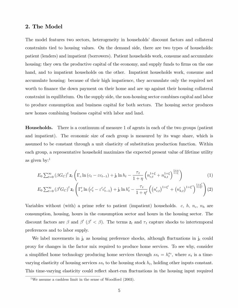
each group, a representative household maximizes the expected present value of lifetime utility

as given by:1

E0P1

t=0 (�GC)t zt

��c ln (ct � "ct�1) + jt lnht �

� t1 + �

�n1+�c;t + n

1+�h;t

� 1+�1+�

�(1)

E0P1

t=0 (�0GC)

tzt

�0c ln

�c0t � "0c0t�1

�+ jt lnh

0t �

� t1 + �0

��n0c;t�1+�0

+�n0h;t�1+�0� 1+�0

1+�0

!.(2)

Variables without (with) a prime refer to patient (impatient) households. c, h; nc; nh are

consumption, housing, hours in the consumption sector and hours in the housing sector. The

discount factors are � and �0 (�0 < �). The terms zt and � t capture shocks to intertemporal

preferences and to labor supply.

We label movements in jt as housing preference shocks, although �uctuations in jt could

proxy for changes in the factor mix required to produce home services. To see why, consider

a simpli�ed home technology producing home services through sst = h�tt , where �t is a time-

varying elasticity of housing services sst to the housing stock ht, holding other inputs constant.

This time-varying elasticity could re�ect short-run �uctuations in the housing input required

1We assume a cashless limit in the sense of Woodford (2003).

5

to produce a given unit of housing services:2 if the utility depends on the service �ow from

housing, the home technology shock looks like a housing preference shock in the reduced-form

utility function.3 The shocks follow:

ln zt = �z ln zt�1 + uz;t; ln � t = �� ln � t�1 + u�;t; ln jt =�1� �j

�ln j + �j ln jt�1 + uj;t

where uz;t, u�;t and uj;t are i.i.d. processes with variances �2z; �2� and �

2j . Above, " measures

habits in consumption,4 and GC is the growth rate of consumption in the balanced growth path.

The scaling factors �c = (GC � ") = (GC � �"GC) and �0c = (GC � "0) = (GC � �0"0GC) ensurethat the marginal utilities of consumption are 1=c and 1=c0 in the steady state.

The log-log speci�cation of preferences for consumption and housing reconciles the trend in

the relative housing prices and the stable nominal share of expenditures on household investment

goods, as in Davis and Heathcote (2005) and Fisher (2007). The speci�cation of the disutility

of labor (�; � � 0) follows Horvath (2000) and allows for less than perfect labor mobility acrosssectors. If � and �0 equal zero, hours in the two sectors are perfect substitutes. Positive values

of � and �0 (as Horvath found) allow for some degree of sector speci�city and imply that relative

hours respond less to sectoral wage di¤erentials.

Patient households accumulate capital and houses and make loans to impatient households.

They rent capital to �rms, choose the capital utilization rate and sell the remaining undepre-

ciated capital; in addition, there is joint production of consumption and business investment

goods. Patient households maximize their utility subject to:

ct + kc;t=Ak;t + kh;t + kb;t + qtht + pl;tlt � bt = wc;tnc;t=Xwc;t + wh;tnh;t=Xwh;t

+(Rc;tzc;t + (1� �kc) =Ak;t) kc;t�1 + (Rh;tzh;t + 1� �kh) kh;t�1 + pb;tkb;t �Rt�1bt�1=�t

+(pl;t +Rl;t) lt�1 + qt (1� �h)ht�1 +Divt � �t � a (zc;t) kc;t�1=Ak;t � a (zh;t) kh;t�1. (3)

2As argued by Piazzesi, Schneider and Tuzel (2007), the production of housing services involves in practiceseveral inputs, such as housing capital, maintenance time and materials, proximity to amenities, the nature ofneighbors and the number of people living in a house. Among these inputs, some are �xed in the short run,while others can be adjusted quickly at little cost. Fluctuations in jt can be seen as a modeling device to capturechanges in the mix required to produce housing services which are exogenous to the model.

3This observational equivalence result echoes �ndings from the household production literature; see forinstance Greenwood, Rogerson and Wright (1995). To obtain this result, it is su¢ cient to note that one couldreplace the expression jt lnht in the utility function with & ln sst; where & is a constant measuring the weight onhousing services in the utility function. The two speci�cations are equivalent if sst = h

jt=&t .

4The speci�cation we adopt allows for habits in consumption only. In preliminary estimation attempts, weallowed for habits in housing and found no evidence of them.

6

Patient agents choose consumption ct; capital in the consumption sector kc;t, capital kh;t and

intermediate inputs kb;t (priced at pb;t) in the housing sector, housing ht (priced at qt); land lt

(priced at pl;t), hours nc;t and nh;t; capital utilization rates zc;t and zh;t, and borrowing bt (loans

if bt is negative) to maximize utility subject to (3). The term Ak;t captures investment-speci�c

technology shocks, thus representing the marginal cost (in terms of consumption) of producing

capital used in the non-housing sector.5 Loans are set in nominal terms and yield a riskless

nominal return of Rt. Real wages are denoted by wc;t and wh;t; real rental rates by Rc;t and

Rh;t, depreciation rates by �kc and �kh. The terms Xwc;t and Xwh;t denote the markup (due to

monopolistic competition in the labor market) between the wage paid by the wholesale �rm

and the wage paid to the households, which accrues to the labor unions (we discuss below the

details of nominal rigidities in the labor market). Finally, �t = Pt=Pt�1 is the money in�ation

rate in the consumption sector, Divt are lump-sum pro�ts from �nal good �rms and from labor

unions, �t denotes convex adjustment costs for capital, z is the capital utilization rate that

transforms physical capital k into e¤ective capital zk and a (�) is the convex cost of setting thecapital utilization rate to z. We discuss the properties of �t, a (�) and Divt in Appendix B.6

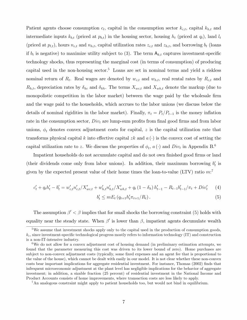
Impatient households do not accumulate capital and do not own �nished good �rms or land

(their dividends come only from labor unions). In addition, their maximum borrowing b0t is

given by the expected present value of their home times the loan-to-value (LTV) ratio m:7

c0t + qth0t � b0t = w0c;tn0c;t=X 0

wc;t + w0h;tn

0h;t=X

0wh;t + qt (1� �h)h0t�1 �Rt�1b0t�1=�t +Div0t (4)

b0t � mEt (qt+1h0t�t+1=Rt) . (5)

The assumption �0 < � implies that for small shocks the borrowing constraint (5) holds with

equality near the steady state. When �0 is lower than �, impatient agents decumulate wealth

5We assume that investment shocks apply only to the capital used in the production of consumption goods,kc, since investment-speci�c technological progress mostly refers to information technology (IT) and constructionis a non-IT-intensive industry.

6We do not allow for a convex adjustment cost of housing demand (in preliminary estimation attempts, wefound that the parameter measuring this cost was driven to its lower bound of zero). Home purchases aresubject to non-convex adjustment costs (typically, some �xed expenses and an agent fee that is proportional tothe value of the house), which cannot be dealt with easily in our model. It is not clear whether these non-convexcosts bear important implications for aggregate residential investment. For instance, Thomas (2002) �nds thatinfrequent microeconomic adjustment at the plant level has negligible implications for the behavior of aggregateinvestment; in addition, a sizable fraction (25 percent) of residential investment in the National Income andProduct Accounts consists of home improvements, where transaction costs are less likely to apply.

7An analogous constraint might apply to patient households too, but would not bind in equilibrium.

7

quickly enough to some lower bound and, for small shocks, the lower bound is binding.8 Patient

agents own and accumulate all the capital. Impatient agents accumulate only housing, and they

borrow the maximum possible amount against it. Along the equilibrium path, �uctuations in

housing values a¤ect, through (5) ; the borrowing and the spending capacity of constrained

households. The e¤ect is larger the larger m; since m measures, ceteris paribus, the liquidity

of housing wealth.

Technology. To introduce price rigidity in the consumption sector, we di¤erentiate between

competitive �exible price/wholesale �rms that produce wholesale consumption goods and hous-

ing using two technologies, and a �nal good �rm (described below) that operates in the consump-

tion sector under monopolistic competition. Wholesale �rms hire labor and capital services and

purchase intermediate goods to produce wholesale goods Yt and new houses IHt: They solve:9

maxYtXt

+qtIHt� Pi=c;h

wi;tni;t +Pi=c;h

w0i;tn0i;t +Rc;tzc;tkc;t�1 +Rh;tzh;tkh;t�1 +Rl;tlt�1 + pb;tkb;t

!.

Above, Xt is the markup of �nal goods over wholesale goods. The production technologies are:

Yt =�Ac;t

�n�c;tn

01��c;t

��1��c (zc;tkc;t�1)�c (6)

IHt =�Ah;t

�n�h;tn

01��h;t

��1��h��b��l (zh;tkh;t�1)�h k�bb;tl�lt�1. (7)

In (6), the consumption sector uses labor and capital to produce the �nal output. In (7),

the housing sector uses labor, capital, land l and the intermediate input kb produced in the

consumption sector. Ac;t and Ah;t measure productivity in the non-housing and housing sector,

respectively. Along the equilibrium path, a rise in Ac;t relative to Ah;t will cause an increase in

the relative price of housing.

As shown by (6) and (7), we let hours of the two households enter the two production

functions in a Cobb-Douglas fashion. This assumption implies complementarity across the

8The extent to which the borrowing constraint holds with equality in equilibrium mostly depends on thedi¤erence between the discount factors of the two groups and on the variance of the shocks that hit the economy.We have solved simpli�ed, non-linear versions of two-agent models with housing and capital accumulation inthe presence of aggregate risk that allow for the borrowing constraint to bind only occasionally. For discountrate di¤erentials of the magnitude assumed here, impatient agents are always arbitrarily close to the borrowingconstraint (details are available upon request). For this reason, we solve the model linearizing the equilibriumconditions of the model around a steady state with a binding borrowing constraint.

9Our notation for the �rm problem re�ects the equilibrium conditions in the markets for nc; n0c; nh; n0h; kc;

kh; kb; l.

8

labor skills of the two groups and allows obtaining closed-form solutions for the steady state

of the model. With this formulation, the parameter � measures the labor income share of

unconstrained households.10

Nominal Rigidities andMonetary Policy. We allow for price rigidities in the consumption

sector and for wage rigidities in both sectors. We rule out price rigidities in the housing market:

according to Barsky, House and Kimball (2007) there are several reasons why housing might

have �exible prices. First, housing is relatively expensive on a per-unit basis; therefore, if menu

costs have important �xed components, there is a large incentive to negotiate on the price of

this good. Second, most homes are priced for the �rst time when they are sold.

We introduce sticky prices in the consumption sector by assuming monopolistic competi-

tion at the �retail� level and implicit costs of adjusting nominal prices following Calvo-style

contracts. Retailers buy wholesale goods Yt from wholesale �rms at the price Pwt in a com-

petitive market, di¤erentiate the goods at no cost, and sell them at a markup Xt = Pt=Pwt

over the marginal cost. The CES aggregates of these goods are converted back into homoge-

neous consumption and investment goods by households. In each period, a fraction 1 � �� ofretailers set prices optimally, while a fraction �� cannot do so, and index prices to the previous

period in�ation rate with an elasticity equal to ��. These assumptions deliver the following

consumption-sector Phillips curve:

ln �t � �� ln �t�1 = �GC (Et ln �t+1 � �� ln �t)� "� ln (Xt=X) + up;t (8)

where "� =(1���)(1��GC��)

��. Above, i.i.d. cost shocks up;t are allowed to a¤ect in�ation inde-

pendently from changes in the markup. These shocks have zero mean and variance �2p.

We model wage setting in a way that is analogous to price setting. Patient and impatient

households supply homogeneous labor services to unions. The unions di¤erentiate labor services

as in Smets and Wouters (2007), set wages subject to a Calvo scheme and o¤er labor services to

wholesale labor packers who reassemble these services into the homogeneous labor composites

nc; nh; n0c; n

0h.11 Wholesale �rms hire labor from these packers. Under Calvo pricing with

10We have experimented with an alternative setup in which hours of the groups are perfect substitutes inproduction. The results were similar to those reported here. The formulation in which hours are substitutes isanalytically less tractable, since it implies that hours worked by one group will a¤ect total wage income receivedby the other group, thus creating a complex interplay between borrowing constraints and labor supply decisionsof both groups.11We assume that there are four unions, one for each sector/household pair. While unions in each sector

9

partial indexation to past in�ation, the pricing rules set by the union imply four wage Phillips

curves that are isomorphic to the price Phillips curve. These equations are in Appendix B.

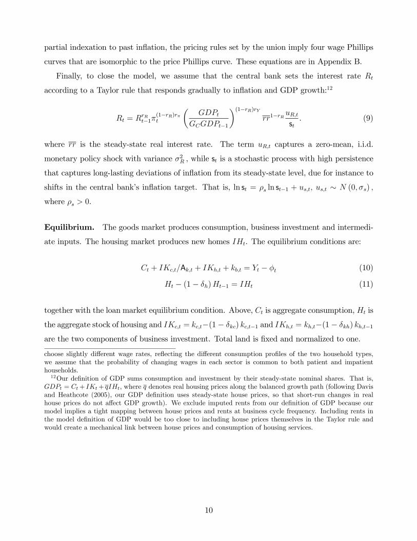
Finally, to close the model, we assume that the central bank sets the interest rate Rt

according to a Taylor rule that responds gradually to in�ation and GDP growth:12

Rt = RrRt�1�

(1�rR)r�t

�GDPt

GCGDPt�1

�(1�rR)rYrr1�rR

uR;tst. (9)

where rr is the steady-state real interest rate. The term uR;t captures a zero-mean, i.i.d.

monetary policy shock with variance �2R , while st is a stochastic process with high persistence

that captures long-lasting deviations of in�ation from its steady-state level, due for instance to

shifts in the central bank�s in�ation target. That is, ln st = �s ln st�1 + us;t; us;t � N (0; �s) ;

where �s > 0.

Equilibrium. The goods market produces consumption, business investment and intermedi-

ate inputs. The housing market produces new homes IHt. The equilibrium conditions are:

Ct + IKc;t=Ak;t + IKh;t + kb;t = Yt � �t (10)

Ht � (1� �h)Ht�1 = IHt (11)

together with the loan market equilibrium condition. Above, Ct is aggregate consumption, Ht is

the aggregate stock of housing and IKc;t = kc;t�(1� �kc) kc;t�1 and IKh;t = kh;t�(1� �kh) kh;t�1are the two components of business investment. Total land is �xed and normalized to one.

choose slightly di¤erent wage rates, re�ecting the di¤erent consumption pro�les of the two household types,we assume that the probability of changing wages in each sector is common to both patient and impatienthouseholds.12Our de�nition of GDP sums consumption and investment by their steady-state nominal shares. That is,

GDPt = Ct+ IKt+ qIHt; where q denotes real housing prices along the balanced growth path (following Davisand Heathcote (2005), our GDP de�nition uses steady-state house prices, so that short-run changes in realhouse prices do not a¤ect GDP growth). We exclude imputed rents from our de�nition of GDP because ourmodel implies a tight mapping between house prices and rents at business cycle frequency. Including rents inthe model de�nition of GDP would be too close to including house prices themselves in the Taylor rule andwould create a mechanical link between house prices and consumption of housing services.

10

Trends and Balanced Growth. We allow for heterogeneous trends in productivity in the

consumption, nonresidential and housing sector. These processes follow:

lnAc;t = t ln (1 + AC) + lnZc;t; lnZc;t = �AC lnZc;t�1 + uC;t

lnAh;t = t ln (1 + AH) + lnZh;t; lnZh;t = �AH lnZh;t�1 + uH;t

lnAk;t = t ln (1 + AK) + lnZk;t; lnZk;t = �AK lnZk;t�1 + uK;t

where the innovations uC;t; uH;t; uK;t are serially uncorrelated with zero mean and standard

deviations �AC ; �AH ; �AK ; and the terms AC ; AH ; AK denote the net growth rates of tech-

nology in each sector. Since preferences and production functions have a Cobb-Douglas form,

a balanced growth path exists, along which the growth rates of the real variables are:13

GC = GIKh= Gq�IH = 1 + AC +

�c1� �c

AK (12)

GIKc = 1 + AC +1

1� �c AK (13)

GIH = 1 + (�h + �b) AC +�c (�h + �b)

1� �c AK + (1� �h � �l � �b) AH (14)

Gq = 1 + (1� �h � �b) AC +�c (1� �h � �b)

1� �c AK � (1� �h � �l � �b) AH . (15)

We note some interesting properties of these growth rates. First, the trend growth rates

of IKh;t; IKc;t=Ak;t and qtIHt are all equal to GC ; the trend growth rate of real consumption.

Second, business investment grows faster than consumption, as long as AK > 0. Third, the

trend growth rate in real house prices o¤sets di¤erences in the productivity growth between the

consumption and the housing sector. These di¤erences are due to the heterogeneous rates of

technological progress in the two sectors and to the presence of land in the production function

for new homes.13Our computational appendix derives the steady state and the balanced growth path of the model. Business

capital includes two components - capital in the consumption sector kc and in the construction sector kh - thatgrow at di¤erent rates (in real terms) along the balanced growth path. The data provide only a chain-weightedseries for the aggregate of these two series, since sectoral data on capital held by the construction sector areavailable only at annual frequency and are not reported in NIPA. Since capital held by the construction sectoris a small fraction of non-residential capital (around 5 percent), total investment is assumed to grow at the samerate as the investment in the consumption-good sector.

11

3. Parameter Estimates

Methods and Data. We linearize the equations describing the equilibrium around the bal-

anced growth path. For given parameter values, the model solution takes the form of a state-

space model that is used to compute the likelihood function. The estimation procedure consists

of transforming the data into a form suitable for computing the likelihood function; choosing

prior distributions for the parameters; and estimating the posterior distribution. Using the

joint probability distribution of data and parameters, one can derive the relationship between

the prior and posterior distribution of the parameters using Bayes�theorem.

We use ten observables: real consumption,14 real residential investment, real business in-

vestment, real house prices,15 nominal interest rates, in�ation, hours and wage in�ation in the

consumption sector, hours and wage in�ation in the housing sector. We estimate the model

from 1965:I to 2006:IV. In Section 5.2, we estimate the model over two subperiods (1965:I to

1982:IV and 1989:I to 2006:IV) in order to investigate the stability of the estimated parameters.

The series (described in Appendix A) are plotted in Figure 1. Real house prices have increased

in the sample period. Business investment has grown faster than consumption, which has in

turn grown faster than residential investment.

We keep the trend and remove the level information from the series that we use in estimation.

In practice, we calibrate depreciation rates, capital shares in the production functions and

weights in the utility functions in order to match consumption, investment and wealth to

output ratios. We also calibrate the discount factor in order to match the real interest rate and

demean in�ation and the nominal interest rate. In a similar vein, we do not use information

on steady-state hours to calibrate the labor supply parameters, since in any multi-sector model

the link between value added of the sector, on the one hand, and available measures of total

14Consumption, investment and hours are in per capita terms, in�ation and the interest rate are expressedon a quarterly basis. We use total chain-weighted consumption, since our goal is to assess the implicationsof housing for a broad measure of consumption, and because chained aggregates do not su¤er the base-yearproblem discussed in Whelan (2003). NIPA data do not provide a chained series for consumption excludinghousing services and durables, which would correspond to our theoretical de�nition of consumption.15We measure house prices using the Census Bureau house price index. Another available house price series

is the repeat sales OFHEO Conventional Mortgage House Price Index (CMHPI), which starts in 1970. In theshort run, the CMHPI moves together with the Census series (the correlation between year-on-year real growthrates of the two series is 0.70). In the 1970-2006 period, the CMHPI has a stronger upward trend: our Censusseries grows in real terms by an average of 1.7 percent per year, the CMHPI by 2.4 percent. Being basedon repeat sales, the CMHPI is perhaps a better measure of house price appreciation at short-run frequencies;however, some have argued that the CMHPI is biased upward (around 0.5 percent per year) because homesthat change hands more frequently have greater price appreciation (see Gallin, 2004). We use the Census seriessince it starts earlier.

12

hours worked in the same sector, on the other, is somewhat tenuous. In addition, there are

reasons to believe that self-employment in construction varies over the cycle. For this reason,

we allow for measurement error in total hours in this sector.16

In equilibrium the transformed variables Ct = Ct=GtC , IHt = IHt=GtIH , IKt = IKt=G

tIK , qt =

qt=Gtq all remain stationary. In addition total hours in the two sectors Nc;t and Nh;t remain

stationary, as do in�ation �t and the nominal interest rate Rt. The model predicts that real

wages in the two sectors should grow at the same rate as consumption along the balanced growth

path. Available industry wage data (such as those provided by the BLS Current Employment

Statistics) show a puzzling divergence between real hourly wages and real consumption over

the sample in question, with the latter rising twice as fast as the former between 1965 and

2006. Sullivan (1997) argues that the BLS measures of sectoral wages su¤er from potential

measurement error. For these two reasons, we use demeaned nominal wage in�ation in the

estimation and allow for measurement error.17

Calibrated Parameters. We calibrate the discount factors �; �0, the weight on housing in

the utility function j, the technology parameters �c; �h; �l; �b; �h; �kc; �kh; the steady-state

gross price and wage markupsX; Xwc, Xwh; the loan-to-value (LTV) ratiom and the persistence

of the in�ation objective shock �s. We �x these parameters because they are either notoriously

di¢ cult to estimate (in the case of the markups) or because they are better identi�ed using

other information (in the case of the factor shares and the discount factors).

Table 1A summarizes our calibration. Table 1B displays the steady-state moments of the

model.18 We set � = 0:9925; implying a steady-state annual real interest rate of 3 percent.

We �x the discount factor of the impatient households �0 at 0:97. This value has a limited

e¤ect on the dynamics but guarantees an impatience motive for impatient households large

enough that they are arbitrarily close to the borrowing limit, so that the linearization around

16Available measures of hours and employment in construction are based on the Current Employment Statis-tics (CES) survey. They classify between (1) residential construction workers, (2) nonresidential constructionworkers and (3) trade contractors, without distinguishing whether trade contractors work in the residential ornonresidential sector. Besides this, the CES survey does not include self-employed and unpaid family workers,who account for about one in three jobs in the construction sector itself, and for much less elsewhere.17We allow for measurement error only on wages in the housing sector. In preliminary estimation attempts,

we also allowed for measurement error for wages in the consumption sector. The estimated standard deviationwas close to zero, and all other parameters were virtually unchanged.18Four of the parameters that we estimate (the three trend growth parameters - AK , AC and AH - and the

income share of patient agents �) slightly a¤ect the steady-state ratios. The numbers in Table 1.B are basedboth on the calibrated parameters and on the posterior estimates reported in Table 2.

13

a steady-state with binding borrowing limit is accurate (see the discussion in Iacoviello, 2005).

We �x X = 1:15; implying a steady-state markup of 15 percent in the consumption-good sector.

Similarly, we set Xwc = Xwh = 1:15: We �x the correlation of the in�ation objective shock �s.

This parameter was hard to pin down in initial estimation attempts; a value of �s = 0:975

implies an annual autocorrelation of trend in�ation around 0.9, a reasonable value.

The depreciation rates for housing, capital in the consumption sector and capital in the

housing sector are set equal, respectively, to �h = 0:01; �kc = 0:025 and �kh = 0:03: The �rst

number (together with j; the weight on housing in the utility function) pins down the ratio of

residential investment to total output at around 6 percent, as in the data. The other numbers

- together with the capital shares in production - imply a ratio of non-residential investment to

GDP around 27 percent. We pick a slightly higher value for the depreciation rate of construction

capital on the basis of BLS data on service lives of various capital inputs, which indicate that

construction machinery (the data counterpart to kh) has a lower service life than other types

of nonresidential equipment (the counterpart to kc).

For the capital share in the goods production function, we choose �c = 0:35. In the housing

production function, we choose a capital share of �h = 0:10 and a land share of �l = 0:10;

following Davis and Heathcote (2005). Together with the other estimated parameters, the

chosen land share implies that the value of residential land is about 50 percent of annual GDP.

This happens because the price of land capitalizes future housing production opportunities.19

We set the intermediate goods share at �b = 0:10. Input-output tables indicate a share of

material costs for most sectors of around 50 percent, which suggests a calibration for �b as high

as 0:50. We choose to be conservative because our value for �b is only meant to capture the

extent to which sticky-price intermediate inputs are used in housing production. The weight

on housing in the utility function is set at j = 0:12. Together with the technology parameters,

these choices imply a ratio of business capital to annual GDP of around 2:1 and a ratio of

housing wealth to GDP around 1:35.

Next, we set the LTV ratio m. This parameter is di¢ cult to estimate without data on debt

and housing holdings of credit-constrained households. Our calibration is meant to measure

the typical LTV ratio for homebuyers who are likely to be credit constrained and borrow the

19Simple algebra shows that the steady-state value of land relative to residential investment equals plqIH =

�l�GC

1��GC. In practice, ownership of land entitles the household to the present discounted value of future income

from renting land to housing production �rms, which is proportional to �l. For �l = 0:10; � = 0:9925;qIH=GDP = 0:06 and our median estimate of GC = 1:0047; this yields the value reported in the main text.

14

maximum possible against their home. Between 1973 and 2006, the average LTV ratio was

0:76.20 Yet �impatient�households might want to borrow more as a fraction of their home.

In 2004, for instance, 27 percent of new homebuyers took LTV ratios in excess of 80 percent,

with an average ratio (conditional on borrowing more than 80 percent) of 0:94. We choose to

be conservative and set m = 0:85. It is conceivable that the assumption of a constant value

for m over a 40-year period might be too strong, in light of the observation that the mortgage

market has become more liberalized over time. We take these considerations into account when

we estimate our model across subsamples, calibrating m di¤erently across subperiods.

Prior Distributions. Our priors are in Tables 2A and 2B. Overall, they are consistent with

previous studies or uninformative. We use uniform priors for the standard errors of the shocks.

For the persistence, we choose a beta-distribution with a prior mean of 0.8 and standard de-

viation of 0.1. We set the prior mean of the habit parameters in consumption (" and "0) at

0.5. For the monetary policy rule, we base our priors on a Taylor rule responding gradually to

in�ation only, so that the prior means of rR; r� and rY are, respectively, 0.75, 1.5 and 0. We

set a prior on the capital adjustment costs of around 10:21 We choose a loose beta prior for the

utilization parameter (�) between zero (capacity utilization can be varied at no cost) and one

(capacity utilization never changes). For the disutility of working, we center the elasticity of

the hours aggregator at 2 (the prior mean for � and �0 is 0.5). We select values for � and �0;

the parameters describing the inverse elasticity of substitution across hours in the two sectors,

of around 1; as estimated by Horvath (2000). We select the prior mean of the Calvo price and

wage parameter ��; �wc and �wh at 0.667, with a standard deviation of 0.05, values that are close

to the estimates of Christiano, Eichenbaum and Evans (2005). The priors for the indexation

parameters ��; �wc and �wh are loosely centered around 0.5, as in Smets and Wouters (2007).

We set the prior mean for the labor income share of unconstrained agents to be 0.65, with

a standard error of 0.05. The mean is in the range of comparable estimates in the literature:

for instance, using the 1983 Survey of Consumer Finances, Jappelli (1990) estimates 20 percent

of the population to be liquidity constrained; Iacoviello (2005), using a limited information

approach, estimates a wage share of collateral-constrained agents of 36 percent.

20The data are from the Federal Housing Finance Board, summary table 19.21Given our adjustment cost speci�cation (see Appendix B), the implied elasticity of investment to its shadow

value is 1= (��) : Our prior implies an elasticity of investment to its shadow price of around 4.

15

Posterior Distributions. Table 2 reports the posterior mean, median and 95 probability

intervals for the structural parameters, together with the mean and standard deviation of the

prior distributions. In addition to the structural parameters, we estimate the standard deviation

of the measurement error for hours and wage in�ation in the housing sector. Draws from the

unknown posterior distribution of the parameters are obtained using the random walk version

of the Metropolis algorithm.22

We �nd a faster rate of technological progress in business investment, followed by consump-

tion and by the housing sector. In the next section, we discuss the implications of these �ndings

for the long-run properties of consumption, housing investment and real house prices.

One key parameter relates to the labor income share of credit-constrained agents. Our

median estimate of � is 0:79 . This number implies a share of labor income accruing to credit-

constrained agents of 21 percent. This value is lower than our prior mean. However, as we

document below, this value is large enough to generate a positive elasticity of consumption to

house prices after a housing demand shock. The dynamic e¤ects of this shock are discussed

more in detail in the next section.

Both agents exhibit a moderate degree of habit formation in consumption and relatively

little preference for mobility across sectors, as shown by the positive values of � (0:67) and �0

(0:99). The degree of habits in consumption is larger for the impatient households ("0 = 0:58,

as opposed to " = 0:33 for the patient ones). One explanation may be that since impatient

households do not hold capital and they cannot smooth consumption through saving, a larger

degree of habits is needed in order to match the persistence of aggregate consumption in the

data. Turning to the labor supply elasticity parameters, the posterior distributions of � and �0

(centered around 0:50) show that the data do not convey much information on these parameters.

We performed sensitivity analysis with respect to these parameters and found that the main

results of the paper are not particularly sensitive for a reasonable range of values of � and �0.

The estimate of �� (0:83) implies that prices are reoptimized once every six quarters. How-

ever, given the positive indexation coe¢ cient (�� = 0:71), prices change every period, although

not in response to changes in marginal costs. As for wages, we �nd that stickiness in the hous-

22Tables and �gures are based on a sample of 200,000 draws (in the computational appendix, we reportestimates based on 5,000,000 draws, which were essentially the same). The jump distribution was chosen to bethe normal one with covariance matrix equal to the Hessian of the posterior density evaluated at the maximum.The scale factor was chosen in order to deliver an acceptance rate between 25 and 30 percent, depending onthe run of the algorithm. Convergence of the algorithm was assessed by comparing the moments computed bysplitting the draws of the Metropolis into two halves.

16

ing sector (�wh = 0:91) is higher than in the consumption sector (�wc = 0:81), although wage

indexation is larger in housing (�wh = 0:42 and �wc = 0:08).

Estimates of the monetary policy rule are in line with previous evidence. Two facts are

worth mentioning: �rst, we �nd a relatively large response to output growth, with rY = 0:51;

second, we tightly identify the response to in�ation, with a coe¢ cient of r� = 1:36. Finally, all

shocks are quite persistent, with autocorrelation coe¢ cients ranging between 0:91 and 0:997.

4. Properties of the Estimated Model

In this section, we discuss the main workings of our model, mostly with reference to housing

demand shocks and monetary shocks. We single these shocks out not only because of their

importance in explaining cyclical movements in housing variables, but also because they nicely

illustrate the functioning of our model economy.

Housing Preference Shock. Figure 2 displays the responses to a housing preference shock

for our baseline estimates. This shock re�ects a preference shift that increases the marginal

utility of housing. One possible interpretation is that the shock captures changes in the ability

to produce housing services induced by �uctuations in home production technology.23 We label

this shock a housing demand shock, since it raises both house prices and the returns to housing

investment, thus causing the latter to rise. The shock also increases the collateral value of con-

strained agents, thus allowing them to increase borrowing and consumption. Since constrained

agents have a high marginal propensity to consume, the e¤ects on aggregate consumption are

positive, even if consumption of the lenders (not plotted) falls.

Figure 2 also displays the responses for three alternative versions of the model in which we

set �p = 0 (�exible prices), �wc = �wh = 0 (�exible wages) and � = 1 (no collateral e¤ects), while

holding the remaining parameters at the benchmark values. As the �gure illustrates, collateral

e¤ects are the key feature of the model that generates a positive and persistent response of

consumption following an increase in housing demand. Absent this e¤ect, in fact, an increase

in the demand for housing would generate an increase in housing investment and housing prices,

but a fall in consumption. Quantitatively, the observed impulse response translates into a �rst-

23It would be tempting to associate this shock with unmodeled bubbles, changes in demographics, the supplyof credit, or the tax treatment of housing. We do not want to pursue this line here, since, if the shock proxiesfor an unmodeled mechanism, policy invariance is not self-evident.

17

year elasticity of consumption to housing prices (conditional on the shock) of around 0.07. This

result mirrors the �ndings of several papers that document positive e¤ects on consumption from

changes in housing wealth (see, for instance, Case, Quigley and Shiller, 2005, and Campbell and

Cocco, 2007). It is tempting to quantitatively compare our results with theirs. However, our

elasticity is conditional to a particular shock, whereas most microeconometric and time-series

studies in the literature try to isolate the elasticity of consumption to housing prices through

regressions of consumption on housing wealth, both of which are endogenous variables in our

model. We return to this issue in the next section.

Next, we consider the response of residential investment. At the baseline estimates, a shift in

housing demand that generates an increase in real house prices of around 1 percent (see Figure

2) causes residential investment to rise by around 3.5 percent. As the �gure illustrates, sticky

wages are crucial here; in particular, the combination of �exible housing prices and sticky wages

in construction makes residential investment very sensitive to changes in demand conditions.

The numbers here can be related to the �ndings of Topel and Rosen (1988), who estimate an

elastic response of new housing supply to changes in prices. Depending on the speci�cations, for

every 1 percent increase in house prices lasting for two years, they �nd that new construction

rises on impact between 1.5 and 3.15 percent.24

Finally, we consider business investment. The impulse response of business investment is

the combined e¤ect of two forces: on the one hand, capital in the construction sector kh rises;

on the other, there is slow and persistent decline in capital in the consumption sector kc, which

occurs since resources are slowly shifted away from one sector to the other. Quantitatively,

the two e¤ects roughly o¤set each other, and the overall response of business investment is

quantitatively small.

Monetary Shock. Figure 3 plots an adverse i.i.d. monetary policy shock. Real house prices

drop and remain below the baseline for about six quarters. The quantitative e¤ect of the

monetary shock on house prices is similar to what is found in VAR-based studies of the impact

of monetary shocks on house prices (see, for instance, Iacoviello, 2005). All components of

aggregate demand fall, with housing investment showing the largest drop, followed by business

investment and consumption. The large drop in housing investment is a well-documented fact

24In other experiments, we have found that larger values of m, the loan-to-value ratio, operate similarly tosmaller values of �. Larger values of m, in particular, work to amplify the response of consumption to monetaryand housing preference shocks.

18

in VAR studies (e.g. Bernanke and Gertler, 1995). As the �gure shows, both nominal rigidities

and collateral e¤ects amplify the response of consumption to monetary shocks. Instead, the

responses of both types of investment are only marginally a¤ected by the presence of collateral

constraints: the reason for this result is, in our opinion, that the model ignores �nancing frictions

on the side of the �rms. In fact, collateral e¤ects slightly reduce the sensitivity of investment

to monetary shocks, since unconstrained households shift loanable funds from the constrained

households towards �rms in order to smooth their consumption. Finally, the negative response

of real house prices to monetary shocks instead mainly re�ects nominal stickiness.

Quantitatively, the response of residential investment is �ve times larger than consumption

and twice as large as business investment. As Figure 3 shows, wage rigidity plays a crucial role.

Housing investment is interest rate sensitive only when wage rigidity is present.25 In particular,

housing investment falls because housing prices fall relative to wages; housing investment falls

a lot because the �ow of housing investment is small relative to its stock, so that the drop

in investment has to be large to restore the desired stock-�ow ratio. Our �ndings therefore

support the models of Barsky, House and Kimball (2007) and Carlstrom and Fuerst (2006),

who show how models with rigid non-durable prices and �exible durable prices may generate a

puzzling increase in durables following a negative monetary shock, and that sticky wages can

eliminate this puzzle.26

Other Shocks. Our �ndings for the responses of aggregate variables to other shocks resemble

those reported in estimated DSGE models that do not include a housing sector (e.g. Smets

and Wouters, 2007, and Justiniano, Primiceri and Tambalotti, 2007).27 We �nd that positive

technology shocks in the non-housing sector drive up both housing investment and housing

prices, whereas analogous shocks in the housing sector lead to a rise in housing investment and

to a drop in housing prices. Temporary cost-push shocks lead to an increase in in�ation and

25In robustness experiments we have found that sectoral wage rigidity (rather than overall wage rigidity)matters for this result. That is, sticky wages in the housing sector and �exible wages in the non-housing sectorare already su¢ cient to generate a large response of residential investment to monetary shocks.26A natural question to ask is the extent to which one can regard construction as a sector featuring strong wage

rigidities. Some evidence, besides our econometric �ndings, seems to point in this direction. First, constructionhas higher than average unionization rates compared to the private sector in general: 15.4 percent vs. 8.6percent. Second, several state and federal wage laws in the construction industry work to insulate movementsin wages from movements in the marginal cost of working. The Davis-Bacon Act, for instance, is a federal lawmandating a prevailing wage standard in publicly funded construction projects; several states have followed withtheir own wage legislation, and the provisions of the Davis-Bacon Act apply to large �rms in the constructionsector, even for private projects.27Our technical appendix plots the impulse responses of the model variables to all the structural shocks.

19

a decline in house prices, whereas persistent shifts in the in�ation target persistently move up

both in�ation and housing prices; hence, depending on how persistent in�ationary surprises are,

they can lead house prices either up or down. In any event, as we discuss in the next section,

these in�ationary surprises do not explain a large fraction of the �uctuations in housing prices.

Coherence of Model with the Data. Our estimated model is capable of accounting well for

the business cycle behavior of housing and non-housing variables. Table 3 reports business cycle

statistics of the model. Most of the model moments lie within the 95 percent probability interval

computed from the data. In particular, the model can replicate the comovement between the

components of aggregate demand, the procyclicality of housing prices and housing investment,

and the relative volatility of our series.28

The Role of Real Rigidities and Land. The introduction of a large number of nominal

and real frictions raises the question as to which role each of them plays. Here, we summarize

our main �ndings. Our estimated model prefers features that slow down sectoral reallocation of

labor and capital. In our setup, labor is not perfectly mobile, capital is sector speci�c and costly

to adjust,29 and the housing sector uses intermediate inputs produced in the other sector. We

have explored speci�cations in which we relax these assumptions. While the qualitative �ndings

are largely unchanged, our estimated model with all real rigidities (partial labor mobility,

habits and variable capacity) can better explain persistence in most series and comovement

across sectors. For instance, by smoothing the response of real marginal costs in response to

changes in demand, variable capacity and adjustment costs can explain the persistence and the

sensitivity of aggregate demand in response to shocks.

A �nal comment concerns the role of land. In our setup, land works in a way similar to an

adjustment cost on housing investment, since it limits the extent to which the housing stock

can be adjusted. In response to shocks, a larger land share reduces the volatility of housing

28In our estimated model, the peak correlation of housing investment with other components of aggregatedemand (consumption and business investment) is the contemporaneous one. This is slightly at odds with thedata, which show that housing investment comoves with consumption but leads business investment. Fisher(2007) develops a model that extends the home production framework to make housing complementary to laborand capital in business production; he shows that in such a model housing investment leads business investment.29We have explored a version of our model with adjustment costs for the changes in business and residential

investment, along the lines of Christiano, Eichenbaum and Evans (2005). The parameter estimates and theimplied sensitivity of consumption to housing shocks were somewhat similar to the version with capital adjust-ment costs. The investment adjustment cost model delivers a smaller sensitivity of residential investment tomonetary shocks (the peak response is three times smaller) and a greater role for housing technology shocks inexplaining �uctuations in housing investment.

20

investment and increases the volatility of prices.

5. Sources and Consequences of Housing Market Fluctuations

Having shown that the estimated model �ts the data reasonably well, we use it to address

the two questions we raised in the introduction. First, what are the main driving forces of

�uctuations in the housing market? Second, can we quantify the spillover e¤ects from the

housing market to the rest of the macroeconomy?

5.1. What Drives the Housing Market?

Trend Movements. We �nd a faster rate of technological progress in business investment,

followed by the consumption sector and, last, by the housing sector. At the posterior median,

the long-run quarterly growth rates of consumption, housing investment and real house prices

(as implied by the values of the terms and equations 12 to 15) are respectively 0:47, 0:15

and 0:32 percent. In other words, the trend rise in real house prices observed in the data

re�ects, according to our estimated model, faster technological progress in the non-housing

sector. As shown in Figure 4, our estimated trends �t well the secular behavior of consumption,

investment and house prices. According to the model, the slow rate of increase of productivity

in construction is behind the secular increase in house prices. Our �nding is in line with the

results of Corrado et al. (2006), who construct sectoral measures of TFP growth for the U.S..

They also �nd that the average TFP growth in the construction sector is negative (�0:5 percent,annualized) and that increases in the contribution of labor and purchased inputs more than

account for real output growth in the sector.30

What about the role of land? At secular frequencies, land is one of the reasons behind the

increase in real house prices, since it acts as a limiting factor in the production of new homes.

Quantitatively, however, the contribution of land appears small. Given our estimate of AH and

the land share in new homes of 10 percent, the limiting role of land taken alone can account

for about 5 percent of the 93 percent increase in real house prices observed in the data.

Business Cycle Movements. Table 4 presents the results from the variance decomposition.

Taken together, demand (housing preference) and supply (housing technology) shocks in the

30Gort, Greenwood and Rupert (1999) �nd a positive rate of technological progress in structures, but theycon�ne themselves to non-residential structures such as roads, bridges and skyscrapers.

21

housing market explain about one-half of the variance in housing investment and housing prices.

The monetary component (the sum of i.i.d. monetary shocks and persistent shifts in the

in�ation target) explains slightly less, around 20 percent. The average variance of the forecast

error of exogenous shocks in the housing sector to the other components of aggregate demand

(consumption and business investment) is instead small. For instance, housing preference shocks

appear to explain less than 1 percent of the variance in consumption and business investment.

A related question is how the di¤erent shocks have contributed to the major housing cycles

in the United States. Figure 5 provides a visual representation. The solid line displays the

detrended historical data, obtained by subtracting from the raw series the deterministic trends

plotted in Figure 2. The other lines show the historical contribution of the three factors under

our estimated parameters. As Figure 5 shows, the period 1965-2006 has witnessed two major

expansions in real housing prices: the �rst from 1976 to 1980, and the second from 2000 to 2005.

In the �rst cycle, housing prices rose by 17 percent above trend between 1976 and 1980 and

dropped by 12 percent between 1980 and 1985 (see Table 5). This price cycle was accompanied

by large swings in residential investment, with no changes between 1976 and 1980, and a 26

percent rise between 1980 and 1985. Monetary actions did not play an important role here.

Instead, the monetary surprises in the 1976-1980 period cooled o¤ the housing price increase,

reducing house prices by 3 percent. At the same time, technology shocks accounted for an

increase in house prices of around 5 percent.

The recent housing price cycle tells a di¤erent story. As shown by Table 5, housing preference

shocks played a major role in the 2000-2005 expansion. In addition, monetary conditions explain

a non-trivial part of the increase in house prices (more than a quarter) and about one-half of

the increase in housing investment. Monetary conditions are also important in ending the boom

in 2005 and 2006. They reduce housing investment and housing prices by 11 and 3 percent,

respectively.

We conclude this subsection relating our results to some recent papers that have emphasized

the role of in�ation in driving �uctuations in housing prices. Brunnermeier and Juilliard (2006)

use a model in which buyers and renters su¤er from money illusion to show how lower in�ation

can tilt preferences from renting toward owning, thus raising house prices when in�ation is low,

and vice versa. Piazzesi and Schneider (2006) build an OLG model to show that the Great

In�ation of the 1970s led to a portfolio shift by making housing more attractive than equity. This

mechanism can explain the housing boom of the 1970s, but it cannot explain the rise in house

22

prices at the turn of the century. The same authors (Piazzesi and Schneider, 2007) construct an

alternative model in which agents who su¤er from in�ation illusion interact with �smart�agents

in markets for nominal assets. Under this assumption, nominal interest rates move with smart

agents�in�ation expectations, and housing booms occur whenever these expectations are either

especially high or low. There are some key di¤erences between our analysis and the studies

above. First, we consider a richer array of shocks that can potentially a¤ect the housing market,

and let the data decide how much each shock contributes: our variance decomposition exercise

shows the shocks that mostly drive in�ation (markup and in�ation target shocks) explain less

than 15 percent of house price �uctuations, thus playing down the role of in�ation disturbances

as a primary source of house price movements. Second, we consider a di¤erent set of nominal

and real frictions.

5.2. How Big Are the Spillovers from the Housing Market?

We now quantify the spillovers from housing to the broader economy. We do so in two steps.

First, we show how our model is consistent with the idea that the conventional wealth e¤ect on

consumption is stronger when collateral e¤ects are present and o¤ers an easy way to measure

the additional strength that collateral e¤ects provide. Second, we provide an in-sample estimate

of the historical role played by collateral e¤ects in a¤ecting U.S. consumption dynamics.

Full Sample Estimates of the Wealth E¤ect. As we explained above, a large part of

the model spillovers occur through the e¤ects that �uctuations in housing prices have on con-

sumption; these e¤ects mostly rely on (and are reinforced by) the degree of �nancial frictions,

as measured by the wage share of credit constrained agents and by the loan-to-value ratio. As

a crude way of measuring the spillovers, we run a basic version of the consumption growth

regression that, starting from the benchmark random walk model, allows for housing wealth to

a¤ect aggregate consumption. In our simulated model output, a basic regression of consumption

growth on lagged growth in housing wealth31 yields (standard errors are in parenthesis):

� lnCt = 0:0041(0:0001)

+ 0:123(0:005)

� lnHWt�1:

31The model variables have been generated using the posterior median of the parameters. An arti�cial sampleof 10,000 observations was generated. We experimented with speci�cations including lagged income, non-housingwealth and interest rates as controls. The coe¢ cients on these variables turned out to be insigni�cant.

23

Interestingly, the coe¢ cients of the arti�cial regression mimic those from the same regression

based on actual data, which gives:

� lnCt = 0:0039(0:0006)

+ 0:122(0:039)

� lnHWt�1.

An advantage of our model is that it allows running counterfactuals. To do so, we run a

regression using the simulated model output in the absence of collateral e¤ects (setting � =

1 ). This regression, perhaps not surprisingly, yields a (statistically) smaller coe¢ cient on

housing wealth, equal to 0:099.32 The comparison between our data-consistent estimate and

the estimate without collateral e¤ects o¤ers a simple way to measure the spillovers from the

housing market to consumption. In practice, it suggests that collateral e¤ects increase the

elasticity of consumption to housing wealth from about 10 to 12.3 percent.

Another message from this section is that our estimate of � allows capturing well the em-

pirical elasticity of consumption to housing wealth, but it should be remembered that, even

without collateral constraints, our model generates a positive correlation between changes in

housing wealth and changes in future consumption. This result suggests that caution should

be taken in using evidence from reduced-form regressions of consumption on housing wealth in

order to assess the importance of collateral e¤ects.

Subsample Estimates: Financial Liberalization and the Historical Contribution of

Collateral E¤ects. In our baseline estimates, we have kept the assumption that the struc-

tural parameters were constant throughout the sample. However, several market innovations

following the �nancial reforms of the early 1980s a¤ected the housing market. Campbell and

Hercowitz (2005), for instance, argue that mortgage market liberalization drastically reduced

the equity requirements associated with collateralized borrowing. More in general, several de-

velopments in the credit market might have enhanced the ability to households to borrow, thus

reducing the fraction of credit constrained households, as pointed out by Dynan, Elmendorf

and Sichel (2006). Motivated by this evidence, we estimate our model across two subperiods,

and use our estimates to measure the feedback from housing market �uctuations to consumer

spending. Following Campbell and Hercowitz (2005), we set a �low� loan-to-value ratio in

the �rst subperiod and a �high�loan-to-value ratio in the second subperiod in order to model

�nancial liberalization in our setup. Namely, we set m = 0:775 in the period 1965:I-1982:IV32The e¤ects are monotone in �. For instance, a regression setting � = 0:50 yields a coe¢ cient of 0:150.

24

and m = 0:925 in the period 1989:I-2006:IV.33 As we mentioned earlier, high loan-to-value

ratios potentially amplify the response of consumption to given �demand�side disturbances;

however, we remain agnostic about the overall importance of collateral e¤ects, by estimating

two di¤erent values of � (as well as all other parameters) for the two subsamples.

Table 6 compares the model estimates for the two subperiods. The late period captures

the high �nancial liberalization period. Most structural parameters do not di¤er signi�cantly

across subperiods, whereas the volatility of most of the shocks seems to have fallen in the second

period. We �nd a signi�cantly lower value for � in the �rst subperiod (0.68) compared to the

second (0.80). However, the smaller share of credit-constrained agents is more than o¤set by

the larger loan-to-value ratio. As shown by Figure 6, consumption responds more to a given

size preference shock in the second period (a similar result holds when comparing monetary

shocks). Hence the estimates suggest that �nancial innovation has reduced the fraction of

credit-constrained people but, at the same time, has increased their sensitivity to given changes

in economic conditions.

Using the subsample estimates, we calculate the counterfactual consumption path in the

absence of collateral constraints (� = 1), and subtract it from actual consumption to measure

the contribution of collateral constraints to U.S. consumption dynamics. Figure 7 presents our

results. In the early period, the contribution of collateral e¤ects to consumption �uctuations

accounts for 4 percent of the total variance34 of year-on-year consumption growth. In the late

period, instead, collateral e¤ects account for a larger share, explaining 12 percent of the total

variance in consumption growth.35 This result mirrors the �ndings of Case, Quigley and Shiller

(2005), who show that the reaction of consumption to house prices increased after 1986, when

tax law changes began to favor borrowing against home equity and when home equity loans

became more widely available.

33The �rst period ends in 1982:IV, in line with evidence dating the beginning of �nancial liberalization withthe Garn-St.Germain Act of 1982, which deregulated the savings and loan industry. The second period startsin 1989:I; this way, we have two samples of equal length and we allow for a transition phase between regimes.34The variance ratios reported in the text are calculated by dividing, in each sample, the variance of con-

sumption growth in the absence of collateral e¤ects by the total variance of consumption growth.35Using the full sample estimates, the variance of consumption growth explained by collateral e¤ects is around

5 percent in both periods.

25

6. Concluding Remarks

Our estimated model accounts well for several features of the data. At cyclical frequencies,

it matches the observation that both housing prices and housing investment are strongly pro-

cyclical, volatile, and sensitive to monetary shocks. Over longer horizons, the model accounts

well for the prolonged rise in real house prices over the last four decades and views this increase

as the consequence of slower technological progress in the housing sector, and the presence of

land (a �xed factor) in the production function for new homes. We have used our model to

address two important questions. First, what shocks drive the housing market at business cycle

frequency? Our answer is that housing demand shocks and housing technology shocks account

for roughly one-quarter each of the cyclical volatility of housing investment and housing prices.

Monetary factors account for slightly less but have played a major role in the housing market

cycle at the turn of the 21st century. Second, do �uctuations in the housing market propagate

to other forms of expenditure? Our answer is that the spillovers from the housing market to

the broader economy are non-negligible, concentrated on consumption rather than business in-

vestment, and have become more important over time, to the extent that �nancial innovation

has increased the marginal availability of funds for credit-constrained agents.

Our model includes several �macro�candidates for explaining movements in housing market

variables (such as in�ation, monetary policy and technology). An important result of our

paper is that, even after taking these candidates into account, exogenous shifts in housing

preferences are still an important source of �uctuations in housing prices. It would be nice to

dig deeper into the structural determinants of these shifts. In the paper, we have proposed one

interpretation in terms of a change in the technology to produce household goods. Obviously,

other hypotheses are equally plausible. For instance, geographical shifts in the population,

changes in demographics and changes in the income distribution, to the extent that individuals

with di¤erent age and income have di¤erent preferences over the relative share of housing in

their consumption basket, might play a similar role. We leave these and other extensions for

future work.

26

References

[1] Barsky, Robert; House, Christopher, and Kimball, Miles. �Sticky Price Models and DurableGoods.�American Economic Review, 2007, 97, pp. 984-998.

[2] Benhabib, Jess, Richard Rogerson, and Randall Wright, �Homework in Macroeconomics:Household Production and Aggregate Fluctuations.� Journal of Political Economy, 99(1991), pp. 1166-1187.

[3] Bernanke, Ben S., and Gertler, Mark. �Inside the Black Box: The Credit Channel ofMonetary Policy Transmission.� Journal of Economic Perspectives, Fall 1995, 9 (4), pp.27-48.

[4] Bouakez, Hafedh; Cardia, Emanuela, and Ruge-Murcia, Francisco. �The Transmission ofMonetary Policy in a Multi-Sector Economy.�University of Montreal, mimeo, 2005.

[5] Brunnermeier, Markus K., and Julliard, Christian. �Money Illusion and Housing Frenzies.�NBER Working Paper No. 12810, December 2006.

[6] Carlstrom, Charles T., and Fuerst, Timothy S. �Co-Movement in Sticky Price Models withDurable Goods.�Federal Reserve Bank of Cleveland Working Paper 0614, November 2006.

[7] Campbell, Je¤rey, and Zvi Hercowitz, �The Role of Collateralized Household Debt inMacroeconomic Stabilization,�NBER Working Paper 11330, 2005.

[8] Campbell, John Y., and Cocco, Joao F., �How Do House Prices A¤ect Consumption?Evidence from Micro Data.�Journal of Monetary Economics, 2007, 54, 591-621.

[9] Case, Karl E.; Quigley, John M., and Shiller, Robert J. �Comparing Wealth E¤ects: TheStock Market versus the Housing Market.�Advances in Macroeconomics, 2005, 5 (1), pp.1-32.

[10] Christiano, Lawrence; Eichenbaum, Martin, and Charles Evans, �Nominal Rigidities andthe Dynamic E¤ects of a Shock to Monetary Policy.�Journal of Political Economy, 2005,113(1), pp. 1-46.

[11] Corrado, Carol; Lengermann, Paul; Bartelsman, Eric, and Beaulieu, J. Joseph. �Model-ing Aggregate Productivity at a Disaggregate Level: New Results for U.S. Sectors andIndustries.�Board of Governors of the Federal Reserve System, mimeo, 2006.

[12] Davis, Morris A., and Heathcote, Jonathan. �Housing and the Business Cycle.� Interna-tional Economic Review, August 2005, 46 (3), pp. 751-784.

[13] Díaz, Antonia, and Luengo-Prado, Maria. �Precautionary Saving and Wealth Distributionwith Durable Goods.�Northeastern University, mimeo, 2005.

[14] Dynan, Karen E.; Elmendorf, Douglas W. and and Sichel, Daniel. �Can Financial Innova-tion Help to Explain the Reduced Volatility of Economic Activity?.�Journal of MonetaryEconomics, 53 (1), 2006, pp. 123-150.

27

[15] Edge, Rochelle; Kiley, Michael T. and Laforte, Jean-Philippe. �An Estimated DSGEModelof the US Economy with an Application to Natural Rate Measures.� Board of Governorsof the Federal Reserve System, mimeo, 2005.

[16] Fisher, Jonas D. M. �Why Does Household Investment Lead Business Investment over theBusiness Cycle?.�Journal of Political Economy, 2007, 115 (1), pp. 141-68.

[17] Gallin, Joshua. �The Long-Run Relationship between House Prices and Rents.�FederalReserve Board of Governors Finance and Economics Discussion Series Paper, 2004.

[18] Gervais, Martin. �Housing Taxation and Capital Accumulation.� Journal of MonetaryEconomics, October 2002, 49 (7), pp. 1461-1489.

[19] Gort, Michael; Greenwood, Jeremy, and Rupert, Peter. �Measuring the Rate of Tech-nological Progress in Structures.�Review of Economic Dynamics, 2, January 1999, pp.207�30.

[20] Greenwood, Jeremy, and Hercowitz, Zvi. �The Allocation of Capital and Time over theBusiness Cycle.�Journal of Political Economy, December 1991, 99 (6), pp. 1188-214.

[21] Greenwood, Jeremy; Hercowitz, Zvi, and Krusell, Per. �The Role of Investment-Speci�cTechnological Change in the Business Cycle.�European Economic Review, January 2000,44 (1), pp. 91-115.

[22] Greenwood, Jeremy; Rogerson, Richard, and Wright, Randall. �Household Productionin Real Business Cycle Theory.� In Thomas Cooley, editor, �Frontiers of Business CycleResearch,�Princeton, N.J.: Princeton University Press (1995), pp. 157�174.

[23] Horvath, Michael. �Sectoral Shocks and Aggregate Fluctuations.� Journal of MonetaryEconomics, February 2000, 45 (1), pp. 69-106.

[24] Iacoviello, Matteo. �House Prices, Borrowing Constraints and Monetary Policy in theBusiness Cycle.�American Economic Review, June 2005, 95 (3), pp. 739-764.

[25] Jappelli, Tullio. �Who Is Credit Constrained in the U.S. Economy?�Quarterly Journal ofEconomics, February 1990, 105 (1), pp. 219-234.

[26] Justiniano, Alejandro; Primiceri, Giorgio, and Tambalotti, Andrea. �Investment Shocksand Business Cycles.�Northwestern University, mimeo, 2007.

[27] Peterson, Brian. �Aggregate Uncertainty, Individual Uncertainty and Illiquidity: Housingand the Business Cycle.�Indiana University, mimeo, 2004.

[28] Piazzesi, Monika, and Schneider, Martin. �In�ation and the Price of Real Assets.�Univer-sity of Chicago, mimeo, 2006.

[29] Piazzesi, Monika, and Schneider, Martin. �In�ation Illusion, Credit, and Asset Prices.�2007, forthcoming in John Y. Campbell (ed.), Asset Prices and Monetary Policy.

[30] Piazzesi, Monika; Schneider, Martin, and Tuzel, Selale. �Housing, Consumption and AssetPricing.�Journal of Financial Economics, 2007, 83, pp. 531-569.

28

[31] Smets, Frank, andWouters, Raf. �Shocks and Frictions in U.S. Business Cycles.�AmericanEconomic Review, June 2007, 97 (3), pp. 586-606.

[32] Sullivan, Daniel. �Trends in Real Wage Growth.�Chicago Fed Letter, Number 115, March1997.

[33] Thomas, Julia K. �Is Lumpy Investment Relevant for the Business Cycle?� Journal ofPolitical Economy, June 2002, 110 (3) pp. 508-34.

[34] Topel, Robert H., and Rosen, Sherwin. �Housing Investment in the United States.�Journalof Political Economy, August 1988, 96(4), pp. 718-40.

[35] Whelan, Karl.�A Two-Sector Approach to Modeling U.S. NIPA Data.�Journal of Money,Credit, and Banking, August 2003, 35 (4), pp. 627-656.

[36] Woodford, Michael. Interest and Prices: Foundations of a Theory of Monetary Policy.Princeton, N.J.: Princeton University Press, 2003.

29

Appendix A. Data and Sources

Aggregate Consumption: Real Personal Consumption Expenditure (seasonally adjusted,billions of chained 2000 dollars, Table 1.1.6), divided by the Civilian Noninstitutional Population(CNP16OV). Source: Bureau of Economic Analysis (BEA).

Business Fixed Investment: Real Private Nonresidential Fixed Investment (seasonally ad-justed, billions of chained 2000 dollars, Table 1.1.6), divided by CNP16OV. Source: BEA.

Residential Investment: Real Private Residential Fixed Investment (seasonally adjusted,billions of chained 2000 dollars, Table 1.1.6.), divided by CNP16OV, logged. Source: BEA.

In�ation: Quarter on quarter log di¤erences in the implicit price de�ator for the nonfarmbusiness sector, demeaned. Source: Bureau of Labor Statistics (BLS).

Nominal Short-term Interest Rate: 3-month Treasury Bill Rate (Secondary Market Rate),expressed in quarterly units, demeaned. (Series ID: H15/H15/RIFSGFSM03_NM). Source:Board of Governors of the Federal Reserve System.

Real House Prices: Census Bureau House Price Index (new one-family houses sold includingvalue of lot) de�ated with the implicit price de�ator for the nonfarm business sector. Source:Census Bureau, http://www.census.gov/const/price_sold_cust.xls. A description of thisprice index is at http://www.census.gov/const/www/descpi_sold.pdf.

Hours in Consumption Sector: Total Nonfarm Payrolls (Series ID: PAYEMS in Saint LouisFed Fred2) less all employees (Series ID: USCONS) in the construction sector, times AverageWeekly Hours of Production Workers (Series ID: CES0500000005), divided by CNP16OV .Demeaned. Source: BLS.

Hours in Housing Sector: All Employees in the Construction Sector (Series ID: USCONSin Saint Louis Fed Fred2), times Average Weekly Hours of Construction Workers (series ID:CES2000000005, source: BLS), divided by CNP16OV. Demeaned.

Wage In�ation in Consumption-good Sector: quarterly changes in Average Hourly Earn-ings of Production/Nonsupervisory Workers on Private Nonfarm Payrolls, Total Private (SeriesID: CES0500000008). Demeaned. Source: BLS.

Wage In�ation in Housing Sector: quarterly changes in Average Hourly Earnings of Pro-duction/Nonsupervisory Workers in the Construction Industry (Series ID: CES2000000008).Demeaned. Source: BLS.

30

Appendix B. The Complete Model

We summarize here the equations describing the equilibrium of the model. Let uc denotethe marginal utility of consumption, unc (unh) the marginal disutility of working in the goods(housing) sector, and uh the marginal utility of housing (with analogous de�nitions holding forimpatient households). We drop the t subscript to denote the steady-state value of a particularvariable.The budget constraint for patient households is:

ct +kc;tAk;t

+ kh;t + kb;t + qtht + pl;tlt � bt =wc;tXwc;t

nc;t +wh;tXwh;t

nh;t

+

�Rc;tzc;t +

1� �kcAk;t

�kc;t�1 + (Rh;tzh;t + 1� �kh) kh;t�1 + pb;tkb;t �

Rt�1bt�1�t

+(pl;t +Rl;t) lt�1 + qt (1� �h)ht�1 +Divt � �t �a (zc;t)

Ak;tkc;t�1 � a (zh;t) kh;t�1. (A.1)

The corresponding �rst-order conditions for patient households are:

uc;tqt = uh;t + �GCEt (uc;t+1qt+1 (1� �h)) (A.2)

uc;t = �GCEt (uc;t+1Rt=�t+1) (A.3)

uc;t

�1

Ak;t+@�c;t@kc;t

�= �GCEt

�uc;t+1

�Rc;t+1zc;t+1 �

a (zc;t)

Ak;t+1� �kcAk;t+1

�@�c;t+1@kc;t

��(A.4)

uc;t

�1 +

@�h;t@kh;t

�= �GCEt

�uc;t+1

�Rh;t+1zh;t+1 � a (zh;t) + 1� �kh �

@�h;t+1@kh;t

��(A.5)

uc;twc;t = unc;tXwc;t (A.6)

uc;twh;t = unh;tXwh;t (A.7)

uct (pbt � 1) = 0 (A.8)

RctAkt = a0 (zct) (A.9)

Rht = a0 (zht) (A.10)

uc;tpl;t = �GCEtuc;t+1 (pl;t+1 +Rl;t+1) . (A.11)

The budget and borrowing constraint for impatient households are:

c0t + qth0t =

w0c;tX 0wc;t

n0c;t +w0h;tX 0wh;t

n0h;t + b0t �

Rt�1�t

b0t�1 + qt (1� �h)h0t�1 +Div0t (A.12)

b0t = mEt (qt+1h0t�t+1=Rt) (A.13)

31

and the �rst-order conditions are:

uc0;tqt = uh0;t + �0GCEt (uc0;t+1 (qt+1 (1� �h))) + Et

��tmtqt+1�t+1

Rt

�(A.14)

uc0;t = �0GCEt

�uc0;t+1

Rt�t+1

�+ �t (A.15)

uc0;tw0c;t = unc0;tX

0wc;t (A.16)

uc0;tw0h;t = unh0;tX

0wh;t (A.17)

where �t denotes the multiplier on the borrowing constraint, which is greater than zero in aneighborhood of the equilibrium.The production technologies are (normalizing land to unity):

Yt =�Ac;t

�n�c;tn

01��c;t

��1��c (zc;tkc;t�1)�c (A.18)

IHt =�Ah;t

�n�h;tn

01��h;t

��1��h��l��b k�bb;t (zh;tkh;t�1)�h . (A.19)

The �rst-order conditions for the wholesale goods �rms will be

(1� �c)�Yt = Xtwc;tnc;t (A.20)

(1� �c) (1� �)Yt = Xtw0c;tn

0c;t (A.21)

(1� �h � �l � �b)�qtIHt = wh;tnh;t (A.22)

(1� �h � �l � �b) (1� �) qtIHt = w0h;tn0h;t (A.23)

�cYt = XtRc;tzc;tkc;t�1 (A.24)

�hqtIHt = Rh;tzh;tkh;t�1 (A.25)

�lqtIHt = Rl;tlt�1 (A.26)

�bqtIHt = pb;tkb;t. (A.27)

The Phillips curve is:

ln �t � �� ln �t�1 = �GC (Et ln �t+1 � �� ln �t)� "� ln (Xt=X) + up;t. (A.28)

Denote with !i;t nominal wage in�ation, that is, !i;t = wi;t � wi;t�1 + �t for each sec-tor/household pair. The four wage equations are:

!c;t � �wc ln �t�1 = �GC (Et!c;t+1 � �wc ln �t)� "wc ln (Xwc;t=Xwc) (A.29)

!0c;t � �wc ln �t�1 = �0GC�Et!

0c;t+1 � �wc ln �t

�� "0wc ln (Xwc;t=Xwc) (A.30)

!h;t � �wh ln �t�1 = �GC (Et!h;t+1 � �wh ln �t)� "wh ln (Xwh;t=Xwh) (A.31)

!0h;t � �wh ln �t�1 = �0GC�Et!

0h;t+1 � �wh ln �t

�� "0wh ln (Xwh;t=Xwh) (A.32)

where "wc = (1� �wc) (1� �GC�wc) =�wc; "0wc = (1� �wc) (1� �0GC�wc) =�wc"wh = (1� �wc) (1� �GC�wc) =�wc and "0wh = (1� �wh) (1� �0GC�wh) =�wh.The Taylor rule is:

Rt = (Rt�1)rR �

r�(1�rR)t

�GDPt

GCGDPt�1

�rY (1�rR)rr1�rR

uR;tst

(A.33)

32

where GDPt is the sum of the value added of the two sectors, that is GDPt = Yt� kb;t + qIHt:Two market-clearing conditions are

Ct + IKc;t=Ak;t + IKh;t + kb;t = Yt � �t (A.34)

ht + h0t � (1� �h)

�ht�1 + h

0t�1�= IHt. (A.35)

By Walras�law, bt + b0t = 0: Finally, total land is normalized to unity:

lt = 1. (A.36)

In equilibrium, dividends paid to households equal respectively:

Divt =Xt � 1Xt

Yt +Xwc;t � 1Xwc;t

wc;tnc;t +Xwh;t � 1Xwh;t

wh;tnh;t

Div0t =X 0wc;t � 1X 0wc;t

w0c;tn0c;t +

X 0wh;t � 1X 0wh;t

w0h;tn0h;t.

In addition, we specify the functional forms for the capital adjustment cost and the utilizationrate as:

�t =�kc2GIKc

�kc;tkc;t�1

�GIKc

�2kc;t�1

(1 + AK)t +

�kh2GIKh

�kh;tkh;t�1

�GIKh

�2kh;t�1

a (zc;t) = Rc�$z2c;t=2 + (1�$) zc;t + ($=2� 1)

�a (zh;t) = Rh

�$z2h;t=2 + (1�$) zh;t + ($=2� 1)

�where Rc and Rh are the steady-state values of the rental rates of the two types of capital. Inthe estimation of the model, we specify our prior for the curvature of the capacity utilizationfunction in terms of � = $= (1 +$) : With this change of variables, � is bounded between 0and 1, since $ is positive: values of � close to unity imply that the cost of adjusting capacitybecomes arbitrarily large.Equations A.1 to A.36 together with the values for IKc, IKh, GDPt, �t; a (z), Divt and

Div0t and the laws of motion for the exogenous shocks (reported in the main text) de�ne asystem of 36 equations in the following variables:Patient households: c h kc kh kb nc nh b l zc zhImpatient households: c0 h0 n0c n0h b0

Firms: IH YMarkets/prices: q R � � X wc wh w0c w0h Xwc Xwh X 0

wh X 0wh Rc Rh Rl pb pl.

After detrending the variables by their balanced growth trends, we linearize the resultingsystem around the non-stochastic steady-state and compute the decision rules using standardmethods.

33

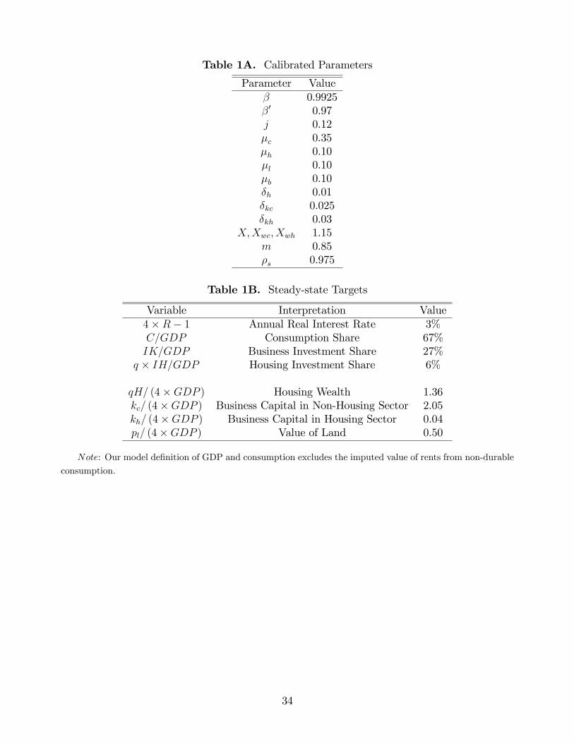
Table 1A. Calibrated Parameters

Parameter Value� 0.9925�0 0.97j 0.12�c 0.35�h 0.10�l 0.10�b 0.10�h 0.01�kc 0.025�kh 0.03

X;Xwc; Xwh 1.15m 0.85�s 0.975

Table 1B. Steady-state Targets

Variable Interpretation Value4�R� 1 Annual Real Interest Rate 3%C=GDP Consumption Share 67%IK=GDP Business Investment Share 27%

q � IH=GDP Housing Investment Share 6%

qH= (4�GDP ) Housing Wealth 1.36kc= (4�GDP ) Business Capital in Non-Housing Sector 2.05kh= (4�GDP ) Business Capital in Housing Sector 0.04pl= (4�GDP ) Value of Land 0.50

Note: Our model de�nition of GDP and consumption excludes the imputed value of rents from non-durable

consumption.

34

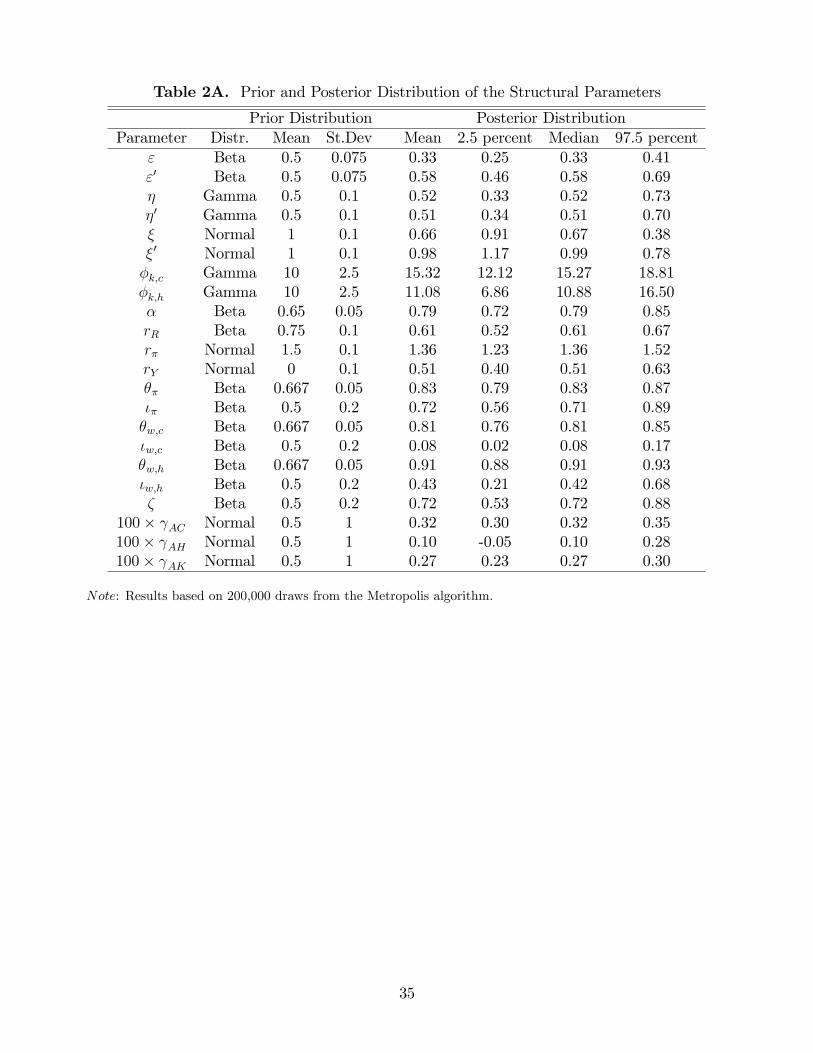
Table 2A. Prior and Posterior Distribution of the Structural Parameters

Prior Distribution Posterior DistributionParameter Distr. Mean St.Dev Mean 2.5 percent Median 97.5 percent

" Beta 0.5 0.075 0.33 0.25 0.33 0.41"0 Beta 0.5 0.075 0.58 0.46 0.58 0.69� Gamma 0.5 0.1 0.52 0.33 0.52 0.73�0 Gamma 0.5 0.1 0.51 0.34 0.51 0.70� Normal 1 0.1 0.66 0.91 0.67 0.38�0 Normal 1 0.1 0.98 1.17 0.99 0.78�k;c Gamma 10 2.5 15.32 12.12 15.27 18.81�k;h Gamma 10 2.5 11.08 6.86 10.88 16.50� Beta 0.65 0.05 0.79 0.72 0.79 0.85rR Beta 0.75 0.1 0.61 0.52 0.61 0.67r� Normal 1.5 0.1 1.36 1.23 1.36 1.52rY Normal 0 0.1 0.51 0.40 0.51 0.63�� Beta 0.667 0.05 0.83 0.79 0.83 0.87�� Beta 0.5 0.2 0.72 0.56 0.71 0.89�w;c Beta 0.667 0.05 0.81 0.76 0.81 0.85�w;c Beta 0.5 0.2 0.08 0.02 0.08 0.17�w;h Beta 0.667 0.05 0.91 0.88 0.91 0.93�w;h Beta 0.5 0.2 0.43 0.21 0.42 0.68� Beta 0.5 0.2 0.72 0.53 0.72 0.88

100� AC Normal 0.5 1 0.32 0.30 0.32 0.35100� AH Normal 0.5 1 0.10 -0.05 0.10 0.28100� AK Normal 0.5 1 0.27 0.23 0.27 0.30

Note: Results based on 200,000 draws from the Metropolis algorithm.

35

Table 2B. Prior and Posterior Distribution of the Shock Processes

Prior Distribution Posterior DistributionParameter Distr. Mean St. Dev. Mean 2.5 percent median 97.5 percent�AC Beta 0.8 0.1 0.95 0.92 0.95 0.97�AH Beta 0.8 0.1 0.997 0.99 0.997 0.999�AK Beta 0.8 0.1 0.93 0.89 0.93 0.96�j Beta 0.8 0.1 0.95 0.91 0.95 0.98�z Beta 0.8 0.1 0.98 0.94 0.99 1.00�� Beta 0.8 0.1 0.91 0.86 0.91 0.95�AC Uniform[0,0.2] 0.0101 0.0089 0.0101 0.0115�AH Uniform[0,0.2] 0.0196 0.0175 0.0195 0.0218�AK Uniform[0,0.2] 0.0111 0.0088 0.0110 0.0138�j Uniform[0,0.2] 0.0462 0.0274 0.0444 0.0771�R Uniform[0,0.2] 0.0034 0.0028 0.0033 0.0041�z Uniform[0,0.2] 0.0437 0.0132 0.0447 0.0768�� Uniform[0,0.2] 0.0287 0.0200 0.0281 0.0397�p Uniform[0,0.2] 0.0047 0.0040 0.0047 0.0054�s Uniform[0,0.2] 0.0003 0.0002 0.0003 0.0004�n;h Gamma 0.001 0.01 0.1203 0.1078 0.1199 0.1360�w;h Gamma 0.001 0.01 0.0071 0.0063 0.0071 0.0081

Note: Results based on 200,000 draws from the Metropolis algorithm.

36

Table 3. Business Cycle Properties of the Model

Model DataMedian 2.5 percent 97.5 percent

Standard deviation (percent)C 1.59 1.21 2.07 1.22IH 8.50 6.79 10.63 9.97IK 4.04 3.16 5.18 4.87q 2.19 1.75 2.73 1.87� 0.49 0.41 0.60 0.40R 0.32 0.25 0.41 0.32GDP 2.22 1.72 2.88 2.17

CorrelationsC;GDP 0.87 0.75 0.93 0.88IH;GDP 0.64 0.43 0.79 0.78IK;GDP 0.89 0.80 0.94 0.75q;GDP 0.67 0.45 0.81 0.58q; C 0.58 0.31 0.76 0.48q; IH 0.48 0.20 0.69 0.41

Note: The statistics are computed using a random selection of 1,000 draws from the posterior distribution and,

for each of them, 100 arti�cial time series of the main variables of length equal to that of the data, giving

a sample of 100,000 series. The business cycle component of each simulated series is extracted using the HP

�lter (with smoothing parameter set to 1,600). Summary statistics of the posterior distribution of the moments

are computed by pooling together all the simulations. GDP denotes domestic demand excluding government

purchases and investment, chained 2000 dollars.

Table 4. Decomposition of the Asymptotic Variance of the Forecast Error

uC uH uK uj uR uz u� up usC 18.8 1.0 0.9 0.3 18.7 8.9 18.9 22.1 9.3IH 3.2 29.3 0.6 27.7 15.0 8.9 6.8 3.9 3.9IK 9.3 0.1 34.4 0.1 14.5 7.5 9.0 17.6 6.7q 8.6 19.0 0.6 26.3 11.4 10.9 6.0 12.5 3.8� 4.7 0.1 0.5 0.4 5.2 2.6 2.9 59.4 23.9R 3.9 0.6 9.3 3.9 19.6 5.3 5.4 17.1 33.4

GDP 15.8 0.9 8.2 2.1 21.5 1.5 19.1 21.9 9.0

Note: The table reports the posterior median value of the variance of the forecast errors at business cycle

frequencies (extracted using the HP �lter with smoothing parameter equal to 1,600).

37

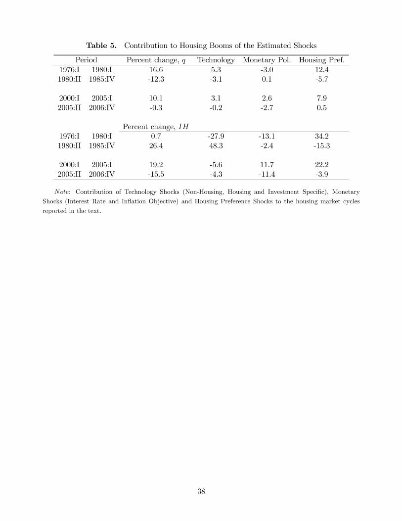
Table 5. Contribution to Housing Booms of the Estimated Shocks

Period Percent change, q Technology Monetary Pol. Housing Pref.1976:I 1980:I 16.6 5.3 -3.0 12.41980:II 1985:IV -12.3 -3.1 0.1 -5.7

2000:I 2005:I 10.1 3.1 2.6 7.92005:II 2006:IV -0.3 -0.2 -2.7 0.5

Percent change, IH1976:I 1980:I 0.7 -27.9 -13.1 34.21980:II 1985:IV 26.4 48.3 -2.4 -15.3

2000:I 2005:I 19.2 -5.6 11.7 22.22005:II 2006:IV -15.5 -4.3 -11.4 -3.9

Note: Contribution of Technology Shocks (Non-Housing, Housing and Investment Speci�c), Monetary

Shocks (Interest Rate and In�ation Objective) and Housing Preference Shocks to the housing market cycles

reported in the text.

38

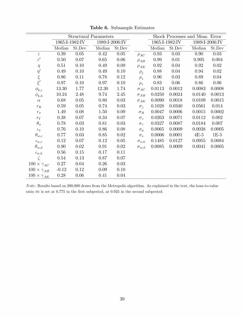
Table 6. Subsample Estimates

Structural Parameters Shock Processes and Meas. Error1965:I-1982:IV 1989:I-2006:IV 1965:I-1982:IV 1989:I-2006:IVMedian St.Dev Median St.Dev Median St.Dev Median St.Dev

" 0.39 0.05 0.42 0.05 �AC 0.93 0.03 0.90 0.03"0 0.50 0.07 0.65 0.06 �AH 0.99 0.01 0.995 0.004� 0.51 0.10 0.49 0.09 �AK 0.92 0.04 0.92 0.02�0 0.49 0.10 0.49 0.10 �j 0.88 0.04 0.94 0.02� 0.86 0.11 0.78 0.12 �z 0.96 0.03 0.89 0.04�0 0.97 0.10 0.97 0.10 �� 0.83 0.06 0.86 0.06�k;c 13.30 1.77 12.30 1.74 �AC 0.0113 0.0012 0.0083 0.0008�k;h 10.24 2.48 9.74 2.45 �AH 0.0250 0.0024 0.0140 0.0013� 0.68 0.05 0.80 0.03 �AK 0.0090 0.0018 0.0109 0.0015rR 0.59 0.05 0.74 0.03 �j 0.1028 0.0340 0.0561 0.014r� 1.49 0.08 1.50 0.09 �R 0.0047 0.0006 0.0015 0.0002rY 0.38 0.07 0.34 0.07 �z 0.0263 0.0071 0.0112 0.002�� 0.78 0.03 0.81 0.03 �� 0.0327 0.0087 0.0184 0.007�� 0.76 0.10 0.86 0.08 �p 0.0065 0.0009 0.0038 0.0005�w;c 0.77 0.03 0.85 0.02 �s 0.0006 0.0001 4E-5 1E-5�w;c 0.12 0.07 0.12 0.05 �n;h 0.1485 0.0127 0.0955 0.0084�w;h 0.90 0.02 0.91 0.02 �w;h 0.0085 0.0009 0.0041 0.0005�w;h 0.56 0.15 0.17 0.11� 0.54 0.13 0.87 0.07

100� AC 0.27 0.04 0.26 0.03100� AH -0.12 0.12 0.09 0.10100� AK 0.28 0.06 0.41 0.04

Note: Results based on 200,000 draws from the Metropolis algorithm. As explained in the text, the loan-to-value

ratio m is set at 0.775 in the �rst subperiod, at 0.925 in the second subperiod.

39

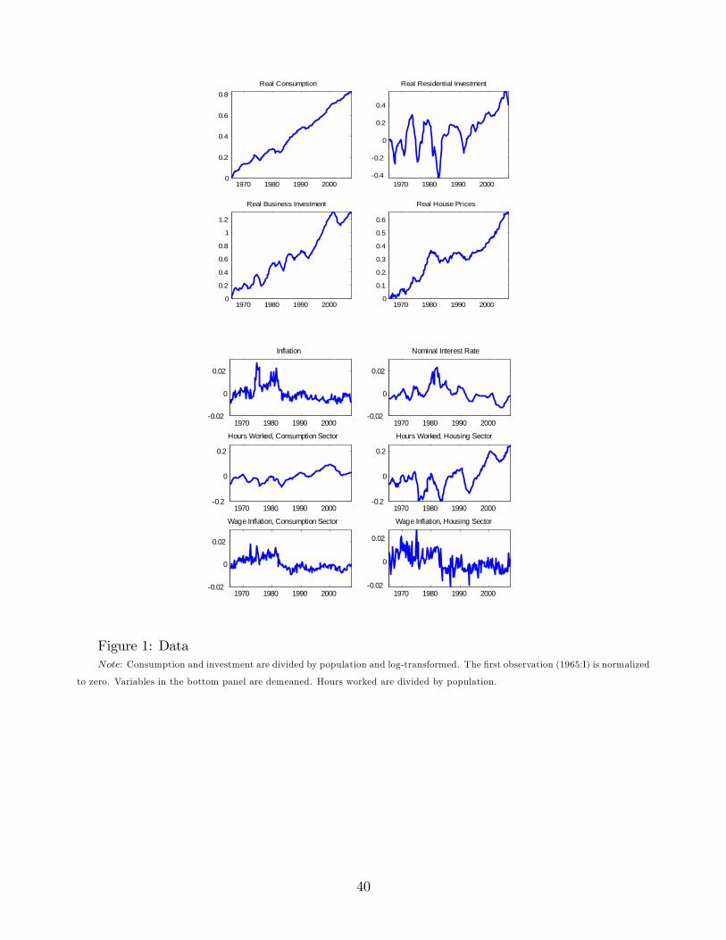
1970 1980 1990 20000

0.2

0.4

0.6

0.8Real Consumption

1970 1980 1990 2000­0.4

­0.2

0

0.2

0.4

Real Residential Investment

1970 1980 1990 20000

0.2

0.4

0.6

0.8

1

1.2

Real Business Investment

1970 1980 1990 20000

0.1

0.2

0.3

0.4

0.5

0.6

Real House Prices

1970 1980 1990 2000­0.02

0

0.02

Inflation

1970 1980 1990 2000­0.02

0

0.02

Nominal Interest Rate

1970 1980 1990 2000­0.2

0

0.2

Hours Worked, Consumption Sector

1970 1980 1990 2000­0.2

0

0.2

Hours Worked, Housing Sector

1970 1980 1990 2000­0.02

0

0.02

Wage Inflation, Consumption Sector

1970 1980 1990 2000­0.02

0

0.02

Wage Inflation, Housing Sector

Figure 1: DataNote: Consumption and investment are divided by population and log-transformed. The �rst observation (1965:I) is normalized

to zero. Variables in the bottom panel are demeaned. Hours worked are divided by population.

40

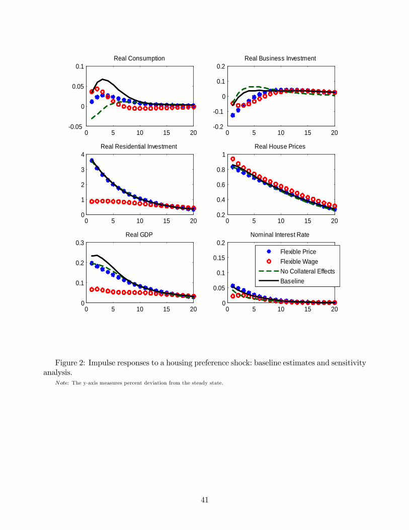
0 5 10 15 20­0.05

0

0.05

0.1Real Consumption

0 5 10 15 20­0.2

­0.1

0

0.1

0.2Real Business Investment

0 5 10 15 200

1

2

3

4Real Residential Investment

0 5 10 15 200.2

0.4

0.6

0.8

1Real House Prices

0 5 10 15 200

0.1

0.2

0.3Real GDP

0 5 10 15 200

0.05

0.1

0.15

0.2Nominal Interest Rate

Flexible PriceFlexible WageNo Collateral EffectsBaseline

Figure 2: Impulse responses to a housing preference shock: baseline estimates and sensitivityanalysis.

Note: The y-axis measures percent deviation from the steady state.

41

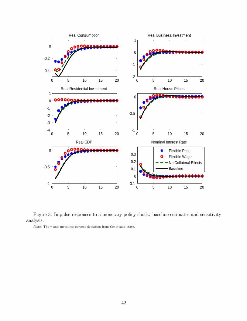
0 5 10 15 20

­0.4

­0.2

0

Real Consumption

0 5 10 15 20­2

­1

0

1Real Business Investment

0 5 10 15 20­4

­3

­2

­1

0

1Real Residential Investment

0 5 10 15 20­1

­0.5

0

Real House Prices

0 5 10 15 20­1

­0.5

0

Real GDP

0 5 10 15 20­0.1

0

0.1

0.2

0.3

Nominal Interest Rate

Flexible PriceFlexible WageNo Collateral EffectsBaseline

Figure 3: Impulse responses to a monetary policy shock: baseline estimates and sensitivityanalysis.

Note: The y-axis measures percent deviation from the steady state.

42

1970 1980 1990 20000

0.2

0.4

0.6

0.8Real Consumption

1970 1980 1990 2000­0.4

­0.2

0

0.2

0.4

Real Residential Investment

1970 1980 1990 20000

0.2

0.4

0.6

0.8

1

1.2

Real Business Investment

1970 1980 1990 20000

0.2

0.4

0.6

Real House Prices

Figure 4: Estimated trendsNote: Dashed lines correspond to the median, 2.5 percentile and 97.5 percentile of the posterior distribution of the trends.

Solid line: data.

43

1965 1970 1975 1980 1985 1990 1995 2000 2005

­0.05

0

0.05

0.1

0.15

Real House Prices

1965 1970 1975 1980 1985 1990 1995 2000 2005

­0.4

­0.2

0

0.2

Real Residential Investment

Housing PreferenceTechnologyMonetary Shocksdata

Figure 5: Historical decomposition of real house prices and real residential investment tohousing preference shocks, technology shocks and monetary shocks. Monetary shocks includei.i.d. monetary policy shocks and changes in the in�ation objective. Technology shocks includehousing, non-housing and investment speci�c technology shocks. All series are in deviationfrom the estimated trend.

Note: Shaded areas indicate recessions as determined by the NBER.

44

0 5 10 15 20­0.05

0

0.05

0.1

0.15Real Consumption

0 5 10 15 20­2

0

2

4

6Real Residential Investment

0 5 10 15 20­0.2

­0.1

0

0.1

0.2Real Business Investment

0 5 10 15 200

0.2

0.4

0.6

0.8

1Real House Prices

1965­19821989­2006

Figure 6: Impulse response functions to a housing preference shock in the two subsamples.The standard error of the preference shock in the second period is normalized so the shocksa¤ect house prices by the same amount in the impact period.

Note: The y-axis measures percent deviation from the steady state.

45

1990 1995 2000 2005

­0.02

0

0.02

0.04

Consumption Growth, ActualConsumption Growth, Contribution of Collateral Effects

1965 1970 1975 1980

­0.02

0

0.02

0.04

Figure 7: The contribution of collateral e¤ects to �uctuations in year-on-year consumptiongrowth: results based on subsample estimates.

Note: The contribution of collateral e¤ects is calculated subtracting from actual consumption growth the path of simulated

consumption growth obtained shutting o¤ collateral e¤ects (setting � = 1 and m = 0). Shaded areas indicate recessions asdetermined by the NBER.

46