how bayes factors change scientific practice...

Journal of Mathematical Psychology 72 (2016) 78–89

Contents lists available at ScienceDirect

Journal of Mathematical Psychology

journal homepage: www.elsevier.com/locate/jmp

How Bayes factors change scientific practiceZoltan Dienes ∗

School of Psychology, University of Sussex, Brighton, BN1 9QH, UKSackler Centre for Consciousness Science, University of Sussex, UK

h i g h l i g h t s

• Bayes factors would help science deal with the credibility crisis.• Bayes factors retain their meaning regardless of optional stopping.• Bayes factors retain their meaning despite other tests being conducted.• Bayes factors retain their meaning regardless of time of analysis.• The logic of Bayes helps illuminate the benefits of pre-registration.

a r t i c l e i n f o

Article history:Available online 7 January 2016

Keywords:Bayes factorNull hypothesisStopping rulePlanned vs post hocMultiple comparisonsConfidence interval

a b s t r a c t

Bayes factors provide a symmetricalmeasure of evidence for onemodel versus another (e.g. H1 versusH0)in order to relate theory to data. These properties help solve some (but not all) of the problems underlyingthe credibility crisis in psychology. The symmetry of the measure of evidence means that there can beevidence for H0 just as much as for H1; or the Bayes factor may indicate insufficient evidence either way.P-values cannotmake this three-way distinction. Thus, Bayes factors indicatewhen the data count againsta theory (and when they count for nothing); and thus they indicate when replications actually supportH0 or H1 (in ways that power cannot). There is every reason to publish evidence supporting the null asgoing against it, because the evidence can bemeasured to be just as strong either way (thus the publishedrecord can be more balanced). Bayes factors can be B-hacked but they mitigate the problem because a)they allow evidence in either direction so people will be less tempted to hack in just one direction; b) asa measure of evidence they are insensitive to the stopping rule; c) families of tests cannot be arbitrarilydefined; and d) falsely implying a contrast is planned rather than post hoc becomes irrelevant (thoughthe value of pre-registration is not mitigated).

© 2015 Elsevier Inc. All rights reserved.

1. Introduction

A Bayes factor is a form of statistical inference in which onemodel, say H1, is pitted against another, say H0. Both models needto be specified, even if in a default way. Significance testing (us-ing only the p-value for inference, as per Fisher, 1935) involvessetting up a model for H0 alone—and yet is typically still used topit H0 against H1. I will argue that significance testing is in thisway flawed, with harmful consequences for the practice of sci-ence (Wagenmakers, 2007). Bayes factors, by specifying two mod-els, resolve several key problems (though not all problems). After

∗ Correspondence to: School of Psychology, University of Sussex, Brighton, BN19QH, UK.

E-mail address: [email protected].

http://dx.doi.org/10.1016/j.jmp.2015.10.0030022-2496/© 2015 Elsevier Inc. All rights reserved.

defining a Bayes factor, the introduction first indicates the generalconsequences of having two models (namely, the ability to obtainevidence for the null hypothesis; and the fact the alternative hasto be specified well enough to make predictions). Then the bodyof the paper explores four ways in which these consequences maychange the practice of science for the better.

1.1. What is a Bayes factor?

In order to define a Bayes factor, the following equation can bederivedwith a few steps from the axioms of probability (e.g. Stone,2013): Normative posterior belief in one theory versus another inthe light of data = a Bayes factor, B × prior belief in one theoryversus another. That is, whatever strength of belief one happenedto have in different theories prior to data (which will be differentfor different people), that belief should be updated by the same

http://dx.doi.org/10.1016/j.jmp.2015.10.003

http://www.elsevier.com/locate/jmp

http://www.elsevier.com/locate/jmp

http://crossmark.crossref.org/dialog/?doi=10.1016/j.jmp.2015.10.003&domain=pdf

mailto:[email protected]


Z. Dienes / Journal of Mathematical Psychology 72 (2016) 78–89 79

amount, B, for everyone.1What this equation tells us is that if wemeasure strength of evidence of data as the amount by whichanyone should change their strength of belief in the two theoriesin the light of the data, then the only relevant information isprovided by the Bayes factor, B (cf Birnbaum, 1962). Conventionalapproximate guidelines for strength of evidence were providedby Jeffreys (1939, though Bayes factors stand on their own ascontinuousmeasures of degrees of evidence). If B > 3 then there issubstantial evidence for H1 rather than H0; if B < 1/3 then thereis substantial evidence for H0 rather thanH1; and if B is in between1/3 and 3 then the evidence is insensitive.

The term ‘prior’ has two meanings in the context of Bayesfactors. P(H1) is a prior probability ofH1, i.e. howmuch youbelievein H1 before seeing the data. But the term ‘prior’ is also used torefer to setting up the model of H1, i.e. to state what the theorypredicts, used for obtaining P(D|H1), the probability of obtainingthe data given the theory. When measuring strength of evidencewith Bayes factors, there is no need to specify priors in the firstsense; but there is a need to specify a model (prior in the secondsense). To know how much evidence supports a theory one mustknow what the theory predicts; but one does not have to knowhowmuch one believes in a theory a priori. In this paper, specifyingwhat a theory predicts will be called a ‘model’.

1.2. The consequences of having two models

The specification of two models in a Bayesian approach, ratherthan one in significance testing, has two direct consequences: Oneis that Bayes factors are symmetric in a way that p-values areasymmetric; and, second, Bayes factors relate theory to data in adirect way that is not possible with p-values. Here I clarify whatthese two properties mean; then the paper will consider in detailhow these properties are important for how we do science.

First, a Bayes factor, unlike a p-value, is a continuous degreeof evidence that can symmetrically favour one model or another(e.g. Rouder, Speckman, Sun, Morey, & Iverson, 2009). Let us callthe models H1 and H0. By using conventional criteria, the Bayesfactor can indicate whether evidence is weak or strong. Thus, theBayes factor may indicate (i) strong evidence for H1 and againstH0; or (ii) strong evidence for H0 and against H1; or (iii) not muchevidence either way. That is a Bayes factor can make a three-way distinction. A p-value, by contrast, is asymmetric. A smallp-value (often) indicates evidence against H0 and for the H1 ofinterest; but a large p-value does not distinguish evidence forH0 from not much evidence for anything. A p-value only tries tomake a two-way distinction: evidence against H0 (i.e. (i)) versusanything else (i.e. (ii) or (iii), without distinguishing them) (andeven this it does not do very well; Lindley, 1957). A large p-valueis, therefore, never in itself evidence for H0. The asymmetry ofp-values leads to many problems that are part of the ‘credibilitycrisis’ in science (Pashler & Wagenmakers, 2012). The reason whyp-values are asymmetric is that they specify only one model: H0.This is their simplicity and hence their beguiling beauty. But theirsimplicity is simplistic. This paper will argue that using Bayesfactors will therefore help solve some (but not all) of the problemsleading to the credibility crisis, by changing scientific practice.

1 In symbols:

P(H1|D)/P(H0|D) = P(D|H1)/P(D|H0) × P(H1)/P(H0)

P(H1)/P(H0) is the ratio of the probabilities (or strength of belief) in H1 versus H0,i.e. the prior odds of H1 versus H0. P(H1/D)/P(H0|D) is the ratio of the probabilitiesof the two theories in the light of the data; i.e. the posterior odds. The remainingterm is the Bayes factor, B, which states that the data are B times more probableunder H1 rather than H0. Briefly, posterior odds = B × prior odds.

The symmetry is particularly important in determining supportfor the null hypothesis, interpreting replications, and p-hacking byoptional stopping, all practical issues discussed below.

The strict use of only onemodel is Fisherian; Neyman and Pear-son (1967) argued that twomodels should be used, and introducedthe concept of power, which helps introduce symmetry in infer-ence, in that it provides grounds for asserting the null hypothesis.Unfortunately power is a flawed solution (Dienes, 2014) and thatmight explain why it is not always taken up. Power cannot be de-termined based on the actual data in order to assess their sensitiv-ity; hence, a highpowerednon-significant resultmight not actuallybe evidence for the null hypothesis, as we shall see. Further, it in-volves (or should involve) specifying only the minimal interestingeffect size, which is a rather incomplete specification of H1 (and itis the aspect of H1 most difficult to make in many cases). In prac-tice, psychologists are happy to assert null hypotheses even whenpower has not been calculated, and inference is based on p-valuesalone (as we shall see).

The second consequence of having to specify H1 as well as H0is that thought must be given to what one’s theory actually pre-dicts (Vanpaemel, 2010). In this way, Bayes factors allow a moreintimate connection between theory and data than p-values allow.This issue is particularly important for dealing with issues of mul-tiple testing and the timing of theorizing versus collecting data. Iconjecture that a Bayesian view of these issues will lead to a moreprobing exploration of theory than significance testing encourages,a point taken up at the end.

The paper now considers in detail the specific changes toscientific practice the use of Bayes factors may bring about.Specifically it considers, in order, issues of obtaining support forthe null hypothesis; of the effect of stopping rules on error rates;of dealing with multiple comparisons in theory evaluation; and,finally, of planned versus post hoc tests and the role of timing oftheory and data in scientific inference. I will argue that Bayesianinference compared to significance testing leads to a re-evaluationof all these issues.

2. Changes to scientific practice

2.1. Supporting the null hypothesis

Here we consider in turn the problem of providing support forthe null hypothesis; how Bayes factors help; andwhy the orthodoxsolution of using power does not solve the problem, as illustratedby high powered attempts to replicate studies.The problem. The key problem created by the asymmetry ofthe p-value is that significance testing per se (i.e. inference byuse of p-values) cannot provide evidence for the null hypothesis.Indeed, that is exactly how p-values are asymmetric. Despite that,a non-significant result is often in practice taken as evidence for anull hypothesis. For example, to take one of the most prestigiousjournals in psychology, in the 2014 April issue of the Journal ofExperimental Psychology: General, in 32 out of the 34 articles, anon-significant result was taken as support for a null hypothesis(as shown by the authors claiming no effect), with no furthergrounds given for accepting the null other than that the p-valuewas greater than 0.05. That is, in the vast majority of the articleswhere there were no grounds for accepting the null hypothesis atall, the null hypothesis was nonetheless accepted, often in order todraw important theoretical conclusions. The effect of this practicecan be disastrous. For example, the drug paroxetine was originallydeclared to have no risk of increased suicide in children becausethe increase of risk was non-significant (it was later shown tohave such a risk, Goldacre, 2013). Human death aside, do we want

80 Z. Dienes / Journal of Mathematical Psychology 72 (2016) 78–89

to guide our theory development partly on conclusions that aregroundless2?

Researchers may know that inferring the null hypothesis froma non-significant result is suspect. That obviously does not stop thepractice from happening, it just makes sure it happens freely in pa-perswhere there also are also key significant results. Butwhere thekey result is non-significant, papers are less likely to be published(Rosenthal, 1979; Simonsohn, Nelson, & Simmons, 2014). The re-search record becomes a misleading representation of the evi-dence. Because the p-value is asymmetric, people seek to get theevidence in the only way it can appear to be strong—as against H0.Thus, apart from failure to publish relevant evidence concerning atheory, another outcome is p-hacking: Pushing the data in the onedirection it can for it to be recognized as strong evidence, by use ofanalytic flexibility (John, Loewenstein, & Prelec, 2012; Masicampo& Lalande, 2012; Simmons, Nelson, & Simonsohn, 2011). No won-der there is a crisis in the credibility of our published results.How Bayes factors help. Bayes factors partly solve the problemby allowing the evidence to go both ways. This means you cantell when there is evidence for the null hypothesis and againstthe alternative. You can tell when there is good evidence againstthere being a treatment side effect (and when the evidence is justweak); you can tell when the data count against a theory (andwhen they count for nothing). There is every reason to publishevidence supporting the null as going against it, because theevidence can be measured to be just as strong either way (thusthe published record can be balanced). In fact, the Bayes factor isthe only way for indicating the strength of evidence for a pointnull hypothesis (though for a Bayes factor H0 need not be a pointvalue; Dienes, 2014; Morey & Rouder, 2011). People can still ‘‘B-hack’’ (i.e. massage data to get a Bayes factor just beyond someconventional threshold by the use of analytic flexibility), but wewill explore how options are more limited than for p-hacking inimportant ways.Power and replication. Replications are hard to evaluate by ref-erence to p-values. If an original result was significant, and adirect replication non-significant, it might feel like a failure toreplicate. But as p-values cannot indicate whether the null hypoth-esis is supported, a non-significant replication tells one nothing initself. This is even true for high powered non-significant replica-tions. The point can be illustrated conceptually by considering ahigh powered replication where both H0 and H1 specify point val-ues. If the sample mean is exactly half way between H0 and H1,then no matter what the power, the data do not discriminate thetheories in any way. In fact, if in a non-significant experiment, thesample mean were closer to H1 than H0, the data would supportH1 more than H0 no matter how highly powered the experiment.Thus, it is rational to consider how the data actually come out toconsider what they say, and power cannot do this.

Most theories allowmore than just one point value; then Bayesfactors can be used to specify the strength of evidence. For ex-ample, consider the Reproducibility Project (https://osf.io/ezcuj/)spearheaded by Brian Nosek (Open Science Collaboration, 2015).The aim was to establish how well 100 experiments publishedin 2008 in high impact journals in psychology replicate, whenthe exact methods specified are followed as closely as possible.In the replication of Correll (2008) by LeBel (https://osf.io/fejxb/wiki/home/), the original ‘‘PSD slope’’ reported in the Correll pa-per (Study 2) was 0.18, SE = 0.077, F(1, 68) = 5.52, p < 0.02.The attempted direct replication doubled sample size to achieve apower of 85%. The slope in the replication was 0.05, SE = 0.056,

2 The sample difference being small, zero, or in the wrong direction does not initself provide sufficient grounds either; see Dienes (2014) for examples.

F(1, 145) = 0.79, p = 0.37. This looks like a ‘‘failure’’ to repli-cate. In fact, calculating a Bayes factor (see Dienes, 2014, 2015, fordetails of how to calculate), BH(0, 0.18) = 0.69, indicating that theevidence is weak and does not substantially support either H0 orH1 (the value of B is between 1/3 and 3).3

In case it is thought that 85% power just is not good enough,consider the replication of Estes, Verges, and Barsalou (2008).These original authors found an incongruent priming conditioncaused more errors than a congruent condition, the differencebeing 4.8%, SE = 1.6%, F(1, 17) = 9.33, p = 0.007. Renkewitz andMuller (https://osf.io/vwnit/) attempted an exact replication witha power of well over 95% for detecting this error difference. In thereplication, they found a difference in errors of 1.4%, SE = 1.1%,F(1, 21) = 1.45, p = 0.24. This is non-significant and hence a‘‘failure’’ to replicate. However, BH(0, 4.8) = 0.79, indicating theevidence was not discriminating between H0 and H1: there are nogrounds for changing one’s confidence in either H0 or H1 to anysubstantial degree based on the replication. On the other hand, itis quite possible to get evidence for the null using a Bayes factorin experiments with such numbers of participants; in the samereplication, the effect on reaction times, which was significant inthe original paper (a 37 ms effect, SE = 6 ms, F(1, 17) = 40.19,p < 0.001), was non-significant in the replication (0.2 ms, SE =

6 ms, F(1, 21) = 0.001, p = 0.5), and also BH(0,37) = 0.19(i.e. B < 1/3), with 22 subjects, indicating substantial support forthe null. The point is that knowing power alone is not enough; oncethe data are in, the obtained evidence needs to be assessed for howsensitively H0 is distinguished from H1, and power cannot do this(Dienes, 2014). (Compare Etz, 2015, for a Bayesian analysis of theexperiments in the Reproducibility Project.)

In sum, Bayes factors would enable amore informed evaluationof replications than p-values allow. The need for more directreplications is clear (Pashler & Harris, 2012); but replications areno good if one cannot properly evaluate the results.

Now we will consider some inferential paradoxes. The asym-metry of p-values leads to a sensitivity to stopping rules which isinferentially paradoxical, because the same data and theories canbe evaluated differently depending on the intentions inside thehead of the experimenter (e.g. Berger & Wolpert, 1988). We nowconsider this and other inferential paradoxes that allow p-hacking.The paradoxes mean that inferential outcome depends on morethan the actual data obtained, and may depend on things whichare in practice unknowable (the intentions and thoughts of exper-imenters; see Dienes, 2011 for explanation). The need to correctfor multiple testing with significance testing is a paradox in thattheories may pass or fail tests on data collected that was irrele-vant to the theory, but corrected for anyway. Instead Bayesian ap-proaches inwhich themodel of H1 is informed by scientific contextfocus only on the relation between theory and the data that bearon specifically that theory. Similarly, the use of timing of theoryversus data as inferentially relevant in itself disguises what is ac-tually very important about pre-registration of studies, as we willdiscuss.

3 Meta-analytic combined estimates should be analysed with Bayes factors too(Dienes, 2014; Rouder &Morey, 2011). In this case, the fixed effect combined meanestimate of Study 2 of Correll (2008) and the replication is 0.095, SE = 0.0453,t(213) = 2.10. In Study 1 of Correll the PDS slope was 0.18; Study 2 soughtto manipulate this slope, and 0.18 remains a useful scale for predicting effects inStudy 2 and the replication. On the combined data of Study 2 and the replication,BH(0, 0.18) = 3.78, substantial support for H1 with all data combined. (BH(0,0.18)indicates that H1 was represented as a half-normal with a mode of zero and astandard deviation of 0.18; that is, the population difference is represented as beingbetween 0 and roughly 2 × 0.18. See Dienes (2014), for explanation.) The Bayesianversion of meta-analysis enjoys all the advantages of Bayesian inference in general;for example, it allows one to obtain support for a null hypothesis, not possible witha meta-analysis using significance testing.

https://osf.io/ezcuj/

https://osf.io/fejxb/wiki/home/






https://osf.io/vwnit/


2.2. The stopping rule

First we consider the problem, how stopping rules influenceerror rates, and thus allow cheating. Then we consider how thisproblem is side-stepped by Bayes factors. Finally, we considerhow stopping rules can lead to biased estimates, and the Bayesiananswer to this problem.The problem. Imagine that after each addition of an observationto data, a p-value is calculated. If H0 is false, the p-value is driventowards small values. However, if H0 is true, the p-value does arandomwalk. That means sooner or later, if H0 is true, the p-valuewill randomly wander below 0.05 (Rouder et al., 2009). So if oneuses significance testing, it is strictly forbidden to keep toppingup participants, without a pre-planned correction. Yet John et al.(2012) estimate that virtually 100% of psychologists at major USuniversities have topped up participants after initially failing toget a significant result. If one decides to continue running untila significant result is obtained, significance is guaranteed even ifH0 is true. Thus, one has to decide on the conditions one wouldstop in advance of collecting data—and then stop at that point. Bycontrast, a Bayes factor B is symmetric. If H0 is false, then, in thelong run, B is driven upwards. If H0 is true, B is driven towards zero.Because B is driven in opposite directions dependent on whichtheory is true, when using a Bayes factor one can stop collectingdata whenever one likes (Savage, 1962). Thus, use of Bayes factorsrespects the ‘‘stopping rule principle’’ according to which the onlyevidence about a parameter is contained in the data and not thestopping rule used to collect them (Berger & Berry, 1988a,b; Berger& Wolpert, 1988).

A useful rule would be to stop collecting data when either Bis greater than 3 or less than 1/3; then one has guaranteed aninformative conclusion with a minimum number of participants(cf. Schoenbrodt,Wagenmakers, Zehetleitner, & Perugini, in press).(Something which power cannot guarantee: A study can be high-powered but still the data do not discriminate between themodels.) While significance testing allows p-hacking by optionalstopping, one cannot B-hack by optional stopping.

The possibility that one can legitimately ignore the stoppingrule would be such a dramatic and useful change to practice, that itmight seem too good to be true. Consider the following argumentfor why the conclusion might be false. The value of B, as anystatistic, is subject to noise, and surely one can capitalize on thatnoise by stopping for example when B > 3 (if it were to be), evenwhen H0 is true? Indeed, Yu, Sprenger, Thomas, and Dougherty(2014) and Sanborn andHills (2014) showed that one could indeedsubstantially raise the false alarm rate for B when H0 was true byusing just such a stopping rule. The effect can be illustrated evenwith a symmetric stopping rule. Imagine an experiment whereeach participant provides a difference score, say their cognitiveperformancewith andwithout a cognitive enhancer.Wehave priorinformation that implies that if there were to be an effect of acognitive enhancer, it would be about one point for the dependentvariable used. Following Dienes (2014), H1 is modelled as a half-normal with an SD of the expected size of effect (i.e. 1). Forsimplicity, assume the population standard deviation of scores is 1.When running for a fixed 100 trials, simulation of the experiment1000 times (see Appendix A for details) showed that when H0 wastrue, B exceeded three 1% of the time, and B was less than a third86% of the time. That is the false alarm rate was only 1%.

Table 1 indicates what happened when the stopping rule wasas follows: After every participant, check to see if either B > 3 orelse B < 1/3. If so, stop. Otherwise run another participant andcontinue until either the threshold is crossed or else 100 subjectsare reached. In terms of researcher practice, this is a worst casescenario; researchers do not typically check after every participant,

but maybe only two or three times when the initial result is non-significant; see Dienes (2011) for why the latter practice is wrongwhen uncorrected for orthodox statistics (and see Sagarin, Ambler,& Lee, 2014, for appropriate corrections). Each number in Table 1is the outcome of 200 simulations. Appendix B gives the R code.Appendix A shows the results for different types of Bayes factors.Notice that when the same threshold for B (i.e. three/a third) isused as for our example with a fixed number of subjects in thelast paragraph, the false alarm rate for when H0was true increasedfrom 1% to 14%. That is, the stopping rule affected the false alarmrate of the Bayes factor. Does this not contradict the claim thatinference using B is immune to the stopping rule?Why the stopping rule is a not a problem for Bayes factors.Rouder (2014) argued elegantly for why the sensitivity of thefalse alarm rate to the stopping rule is consistent with inferencefrom B remaining immune to the stopping rule. Here the sameargument will be put slightly differently. First notice that theequation ‘posterior odds = B ∗ prior odds’ follows from theaxioms of probability. That is, given that the axioms normativelyspecify how the strength of belief should be changed, B isnormatively the amount by which the strength of belief should bechanged regardless of the stopping rule. If strength of evidence ismeasured by howmuch in principle beliefs should normatively bechanged, then B is normatively themeasure of strength of evidencediscriminating two theories. The stopping rule does not come intothe equation, so the claim is true regardless of the stopping rule.But how does this fit with false alarm changing according to thestopping rule?

Notice that B is the measure of evidence regardless of thespecific value of P(D|H0). That is, P(D|H0) can in principle varyas B stays the same. B will still be the measure of strength ofevidence—because P(D|H1) will change by just the right amount.Experimental psychologists are used to such reasoning with signaldetection theory. Discriminability in a perceptual decision taskcan remain the same as bias changes; we would never dream ofmeasuring discriminability by measuring the false alarm rate ina signal detection experiment. Obviously the same point appliesto H0 versus H1. That is, false alarm rate of a procedure canchange when discriminating H0 versus H1 even when the abilityof the procedure to discriminate remains invariant. The evidenceprovided by an observation remains the same even if the criterionis changed (and hence false alarm rate changes). B is the invariantmeasure of the strength of evidence for H1 versus H0, regardless offalse alarm rate.

We as experimental psychologists have become fixed on falsealarm rate for measuring the strength of evidence for a theorybecause we were taught to consider only one model (H0) forsignificance testing. It is like trying to perform signal detectiontheorywith only one distribution, that for noise alone. But in signaldetection theory terms, that is a nonsense; we need the signaldistribution as well. Bayes considers two distributions: One for H0and one for H1. False alarm rate is, by itself, uninformative abouthow well the theories are discriminated.

The Supplementary Materials4 give R code for measuring thefalse alarm and hit rates for Bayes factors for optional stopping.One can vary, amongst other things, the threshold, populationeffect sizes, and theminimumormaximumnumber of participantsbefore optional stopping can begin. Table 2 shows the samesituation as Table 1, but with a minimum of 10 participantsbefore optional stopping could start. The false alarm rate for athreshold of three is halved (see first column in Table 2 comparedto Table 1). B will be most variable early on in testing, because B

4 http://dx.doi.org/10.1016/j.jmp.2015.10.003.













Table 1Per cent decision rates for accepting/rejecting H0 for BH(0,1) (i.e. a Bayes factor in which H1 has been represented as a half-normal,with mode = 0, and SD = 1). Each participant provides a single difference score, sampled from a normal distribution witha standard deviation of 1. Thus, the specified population effect sizes are dz’s (Cohen, 1988). Maximum number of participantsbefore stopping (MaxN) = 100; minimum number of participants before checking after every trial (MinN) = 1. H0 is rejected ifB exceeds the stated threshold, and accepted if B goes below 1/threshold.

Threshold: 3 4 5 6 7 8 9 10

Population effect:dz = 0 Reject H0 14 12 11 11 7 7 6 5

Accept H0 86 87 86 86 85 79 74 69

dz = 1 Reject H0 97 100 100 100 100 100 100 100Accept H0 1 0 0 0 0 0 0 0

Table 2Per cent decision rates for accepting/rejecting H0 for BH(0,1) as for Table 1, except that MinN = 10.

Threshold: 3 4 5 6 7 8 9 10

Population effect:dz = 0 Reject H0 7 7 7 5 5 3 4 3

Accept H0 93 91 88 81 83 82 73 66

dz = 1 Reject H0 100 100 100 100 100 100 100 100Accept H0 0 0 0 0 0 0 0 0

is driven in different directions according to which theory is trueas data accumulates. Once B has picked upmomentum in the rightdirection, it may never exceed a value in the opposite direction,even after an infinite number of participants (Savage, 1962). Thus,having a minimum number of participants, even a small amount,can reduce false alarm rate. Note that B is always and invariablythe correct measure of strength of evidence for discriminatingH0 versus H1, regardless of whether a minimum number ofparticipants is used. Nonetheless if one wanted to control falsealarm rate, in addition to discriminability, the SupplementaryMaterials (see Appendix B) would allow the reader to work outhow to do so by, for example, changing the minimum number ofparticipants, or raising the threshold of B. (There is another reasonto run a minimum number of participants: the validity of theBayes factor, as for any statistical test, depends on the assumptionsof the statistical model of the data being approximately true.A minimum number of participants allows assumptions to bechecked; Morey, Romeijn, & Rouder, 2013). The SupplementaryMaterials (see Appendix B) also provide results for different typesof Bayes factors.

Appendix A illustrates how Bayes factors have better errorproperties as a function of the stopping rule not only than signifi-cance testing, but also than the use of confidence or credibility in-tervals.

In sum, Bayes factors can be used as a measure of evidenceirrespective of the stopping rule, and hence optional stopping isnot a form of B-hacking. In fact stopping when B > 3 or < 1/3(or any other threshold) would enable stopping when the data arejust as discriminating as needed. This guarantees the sensitivity ofa study with a minimum of participants.The issue of bias. It might be argued that, although Bayes factorsare insensitive to the stopping rule as a measure of evidence,the estimates of population values can be biased by the stoppingrule. Thus, we could be in the seemingly awkward position ofhaving fine hypothesis testing but biased parameter estimation,depending on the stopping rule. To illustrate bias arising accordingto the stopping rule, if a researcher was interested in the effectof a drug on mood, she could decide to stop testing after shefound three participants in a row who were happier on the drugthan on placebo. The resulting estimate of how happy the drugmade people would be biased upwards. Bias is a frequentist notionthat therefore needs a reference class to define it; the referenceclass in this case is defined by the stopping rule. That is, let theresearcher repeat the experiment an infinite number of times (and

to allow the argument to be clear, assume the researcher can betaken as randomly sampling from the same population as before),each time stopping the experiment after three participants in arow were happier on the drug than on placebo. Even if the drugwere ineffective, each estimate would have a tendency to indicatethat people were happier on the drug; that is, the mean of all theestimates would show greater happiness on the drug than on theplacebo. Is not this a problem for an experiment, even if analysedby Bayesian statistics?

The clue to the solution is that bias is inherently a frequentistnotion, with need of a reference class (Howson & Urbach, 2006);yet it is the use of reference classes that leads to the inferentialparadoxes in significance testing that do not apply to Bayesiananalyses (Dienes, 2011; Lindley, 1993). Our researcher, as aBayesian, would not simply average the results of the differentexperiments together (in an unweighted way). The experimentsare all basic events in the reference class; but a Bayesiandoes not recognize the reference class as relevant to inference.Note that each experiment would have a different number ofparticipants. The events in the reference class are just one arbitraryway of carving up the full set of data (as given by stringingtogether the infinite number of experiments the researcher runs).Different stopping rules (defining different reference classes)would partition the same full set of data into different events.The same data could be partitioned such that each experimentfinished with three people in a row who were happier on placeborather than drug (now the bias goes the other way). But all thatmatters is the complete data set, not the arbitrary partitionings ofit. The experimenter should combine all her participants together,and then average such that each participant contributes equally.This procedure (of averaging over participants all the data thatone has so far) converges in the limit to the correct value of thepopulation mean (cf Rouder, 2014). The frequentist by contrasthas to work within the reference class predefined by her, and sobias is a genuine worry: By frequentist methods, the average (overreference class events) converges to the correct value only if thestopping rule provides unbiased estimates.5

5 It may seem that the Bayesian solution of weighting according to participantnumber is open to the frequentist; indeed, the frequentist may complain that thesolution I provide above is just as frequentist as Bayesian. But the frequentist isconceptually obliged to respect reference classes even in meta-analyses. ConsiderSmith performing a study which obtained p = 0.08 and publishing. Jones, based


To recap: The stopping rule can introduce bias to estimateswhen the expected value of the estimate is taken over the events ofa reference class. But such bias is irrelevant to Bayesian procedures,whether theory testing (Bayes factors) or estimating populationparameters. Bayes factorswould change scientific practice becausehacking by optional stopping would be ruled out. Given theprevalence of optional stopping (John et al., 2012), this wouldproduce a major change in the robustness of our science.

2.3. Corrections for multiple testing

First we consider the problem that multiple testing givesmultiple opportunities for errors, yet correcting for this introducesinferential arbitrariness; then we consider the Bayesian solution,which removes arbitrariness.The problem. One way people can cheat with inferential statisticsis to make many comparisons and then focus on the one that wassignificant taken on its own. The frequentist solution is to correctfor multiple testing. If with frequentist statistics one decides tocorrect for familywise error rate, the correction depends on anarbitrary specification of what the family is, allowing analyticflexibility (for evidence of wide spread prevalence of problemscreated by flexibility in defining relevant families, see Ioannidis,Munafò, Fusar-Poli, Nosek, & David, 2014; John et al., 2012). WithBayes the issue becomes one of specifying how different theoriesare affected by all the data relevant to them, which is not arbitrary.We consider an imaginary example to illustrate the issues and theirsolution.

An example is now presented in order to consider the issue offamilies of tests. Six studies are run testing the effect of referringto the general concept of ‘‘closing’’ on how quickly a sale is closed(i.e. how quickly the sale is agreed and completed). The maximumtime allocated to the sale was 5 min in each study. A previouspriming study using the same selling paradigm, but priming byseating the client in soft vs. hard chairs, obtained a priming effectof 15 s. Thus, based on the past study, in the current experimentone might expect a priming effect of on the order of magnitudeof roughly 15 s if priming existed (so we can model H1 as a halfnormal with an SD of 15 s, following Dienes, 2014). In one studyfrequent verbal reference was made by the salesperson to closeddoors compared to a control condition; in another condition thesalesperson incidentally discussed Sunday closing rules; and, forexample, in the final study, the salesperson made frequent handgestures reminiscent of a closing door. Each condition had itsown matched control. In one of the studies, the one with handgestures of closing doors, reference to closure indeed resulted infaster closure of the sale as compared to its control condition (withopening hand gestures), mean effect = 10 s, SE = 5 s, t(30) = 2.0,p < 0.05. BH(0,15) = 3.72, indicating substantial evidence for theeffect of priming as opposed to the null hypothesis. None of theother studies were significant, nor had Bayes factors above 3.

A researcher might be tempted to report only the one studythat worked. It did after all involve the most embodied referencesto closing (bodily hand gestures rather than word primes), andit might be presumed, that is why that particular study worked.The other studies, which were all different in a possibly relevant

on Smith’s p-value being tantalizing close to 0.05, runs 20 more participants, andcombines the data together in a meta-analysis. The resulting meta-analytic p =

0.04 is not significant at the 5% level just because it was Jones who topped up andnot Smith (see Section 2.1; so long as Jones topping up is conditional on the p-value obtained by Smith, the overall error rate of the Jones–Smith pair is above5%). Frequentists may intuitively grasp for Bayesian solutions, but that does notmake the frequentist version legitimate (for a similar argument for confidence vs.credibility intervals, see Morey, Hoekstra, Rouder, Lee, & Wagenmakers, in press).

way, had therefore not found the right conditions for eliciting theeffect6. This type of reasoning is very tempting and theremust be aplace for it in exploration. Often researchers explore the conditionsfor eliciting an effect before they find conditions that appearto work. Nonetheless, choosing one study from many is cherrypicking. It is cherry picking because the other studies must havebeen designed in the first place because it was felt they did testthe general theory that priming closure speeds closure. And whenrelevant data have not been reported because the results lookedbetter without them, Bayes factors in themselves cannot makeup for that systematic exclusion. So if only the one ‘‘successful’’study were reported, both Bayesian and conventional statisticswould inappropriately show the evidence to be stronger than itactually was for the general theory that priming ‘‘closing’’ speedsthe closing of sales. (Pre-registration of studies, by itself neitherBayesian nor non-Bayesian, is a key solution to this problem;Wagenmakers, Wetzels, Borsboom, van der Maas, & Kievit, 2012.)That is, bias introduced by the judicious dropping of conditions,discussed by Simmons et al. (2011), is not in itself solved by usingBayesianmethods on the data that remains. Bayesian analyses willnot solve all forms of bias (and then only the ones that are part ofthe formal statistical problem; Jaynes, 2003). A Bayesian analysisrequires that all relevant data are included.

In fact, say that the authors report all studies, so cherry pickingis avoided. What is the evidential value of the final study showingan effect? The orthodox approach corrects for multiple testing.Thus, if all studies are taken as a family, a threshold of 0.05/6 =

0.008may be used for p-values, now rendering the final study non-significant at the 5% level: The presence of an effect cannot beasserted for the embodied priming manipulation. However, froma Bayesian point of view, the evidence provided by the data fromspecifically the final study for thehypothesis that embodiedprimesare effective remains the same, no matter what other proceduresare tested. The Bayes factor remains 3.72 for the evidential worthof the data from the final study, noteworthy evidence for H1concerning this particular procedure. Is this not a problem forBayes?

Before considering the Bayesian solution, first note the flexibil-ity in the frequentist one. Families do not have to be defined by the-oretical question in frequentist statistics, and indeed often are not(theymay e.g. be defined by degrees of freedom in an omnibus test,e.g. Keppel & Zedeck, 1989). By contrast, the Bayesian solution is toconsider the evidence for each theory. In frequentist terms there isno reason why families could not be made of various subsets ofthe studies. In frequentist terms if the sixth study was treated asplanned it could be tested separately from the others, which arethen each corrected at the 0.05/5 level as one family. We will con-sider planned vs. post hoc tests below. For now we consider howBayes just depends on the relation of the data to theories.Whymultiple comparisons are not a problem for Bayes factors.The priming technique used in the final study is a variant of anumber of different priming techniques addressing a commonquestion. Let us say the mean priming effect for the other studieswas 0. Now the overall priming effect across all studies is (10 +

0)/6 = 1.7. For simplicity, assume all studies had identicalstandarddeviations andNs. The standard error for the overallmeaneffect is 5/

√6 = 2.2. Thus, BH(0,15) = 0.30, support for the null

hypothesis that priming closure does not lead to faster closures. Inevaluating the general theory that priming closure speeds closure,all relevant data must be used. And when all data are used, thedata sensitively support the null hypothesis (using for illustration

6 A test of the difference between embodied (mean = 10, SE = 5) and the others(mean = 0, SE = 5/

√5 = 2.2), t(180) = 1.82, ns; BH(0,15) = 2.83, indicates only

anecdotal evidence for a difference.


the guidelines of e.g. Jeffreys, 1939, for interpreting the size ofBayes factors, though note Bayes factors stand by themselves ascontinuous degrees of evidence).

The theory that embodied primes of closure speeds closurecan be regarded as a specific or subordinate level theory of ageneral or superordinate level theory that priming closure speedsclosure. Here the specific theory received substantial evidenceconsidered on its own, while the general theory overall hadsubstantial evidence against it. Naturally, in specific cases evidencepointed in somewhat different directions, as evidence will; buttaken together, the evidencewas clearly against the general theory.Note there was no need to correct for multiple comparisons; wejust had to take account all evidence directly testing a given theory.(Scientific judgement will always determine the relevant specificand general theories.)

Bayes factors enable a properly nuanced extraction of informa-tion from data, unlike significance testing. That is, Bayesian infer-ence reflects the fact there is evidence for a specific theory, whilethe data as a whole count against the more general theory. If onehad independent reasons for thinking embodiment was especiallyimportant for making priming effective, more data could be col-lected, using themanipulation of the final study, until the evidencefor both the subordinate and superordinate theories was convinc-ing one way or the other. That is, publishing support for both thesubordinate and superordinate theories (and showing statisticallythat embodiment was better than non-embodiment) would re-quire more data than currently on the table. On the other hand, ifprevious research indicated that word and embodied primes wereroughly similar in efficacy in other domains, one could simply gowith the evidence for the superordinate theory, and regard it assubstantially weakened by the data.

The same logic can be applied generally to caseswheremultipletests are applied, all bearing on a common superordinate theory.Consider collecting data on a vast number of EEG and ERPmeasures on meditators and matched non-meditators, hoping tofind indicators of superior attentional abilities in meditators thannon-meditators. (So the scientific question has set the relevantsuperordinate hypothesis.) ‘‘Attentional ability’’ could manifestitself in a large number of different ways: More theta density?Larger P300 amplitudes? And on and on. The problem thisdesign raises is that conclusions could rely on cherry picking afew EEG measures that came out as expected, and ignoring allthose that gave non-significant results. Without corrections formultiple testing, how could Bayesian analyses protect againstseeing patterns in noise? Here is one way to proceed. First specifywhich dependent variables measure attention, or the sort ofattention we may be interested in. Then devise a way of meta-analytically combining all those measures into a single one. Finallytest the strength of evidence that the overall measure provides forthe superordinate theory thatmeditators have stronger attentionalskills than non-meditators. Combining evidence is not peculiarlyBayesian (though combining evidence to obtain an overall strengthof evidence is). But the procedure does show why Bayesianinference leads to sensible answers when it comes to multipletesting situations. When our real interest is in a general theory,we must assess all evidence for that theory. By realizing that non-significant results may carry evidential value, Bayesian inferenceencourages researches to use all available data. Significance testingcan encourage ignoring non-significant results as non-evidentialand hence cherry picking the significant ones.7

7 When an informedmodel is tested, Bayesian inference requires one draw on alland only the relevant data. Strange as it is in hindsight, frequentist statistics justhave not operated in that way. Frequentists could copy Bayesians in pooling datarelevant to theories. But why not start from principles that directly lead to the rightanswer, rather than those that underspecify what to do?

For another example, consider finding evidence for a differencein activation between conditions in one tiny voxel in an fMRIstudy. If that voxel is structurally and theoretically arbitrary, itmeans nothing for theory development. Results mean nothingexcept in so far as they inform interesting theory. The question is,when we combine activation across theoretically and structurallymeaningful sets of voxels, what remains of the evidence? (And assoon as you construct a meaningful theory about what is goingon, consider what other voxels are now implicated in testingthe theory. Only when all evidence relevant to the superordinatetheory has been taken into account can the superordinate theorybe evaluated.)

The strategy suggested so far relies on using a Bayes factor totest a single degree-of-freedom hypothesis. This provides a simplebroadly applicable strategy but the use of Bayes factors is notlimited to this strategy. A superordinate theory that specifies arank ordering of means in different conditions can also be testedwith a Bayes factor using the methods of Hoijtink (2011). Forexample, a theory that specified that the mean for the first andsecond conditions should be the same but higher than those from athird, specifies a set of ordinal constraintswhich together are richerthan a single degree-of-freedom comparison. An editor might beespecially prepared to accept a paper in favour of or against asuperordinate theory if the theory received substantial evidenceas a whole (either for or against), regardless of the direction ofspecific cherry-picked comparisons. Of course, the single degreeof freedom comparisons (first mean versus second mean; theiraverage versus the third) would help pinpoint strength of evidencefor specific claims made by the theory.

So far it might be thought that Bayes does little better thansignificance testing in dealing with multiple testing situations(after all, in orthodox statistics one could combine evidence acrosssituations in theory relevant ways). Bear in mind that in Bayesianinference one is not at liberty to define families at will; onehas to ask about the relation of data to each specific theory ofinterest, so ‘‘families’’ must be picked out as the tests relevantto a given theory. Bayesian inference can indicate the supportfor or against any specified theory. But Bayesian inference cando more, by taking into account the full Bayesian apparatus thatlies beyond non-Bayesian approaches. A Bayes factor representsthe strength of evidence data provides for one theory ratherthan another. That evidence informs the posterior probabilitiesfor the different theories. The posterior probability that embodiedpriming of closure is effective may be affected by the evidencefor priming using words; that is, if there is priming for wordsit increases the probability that there could be priming fromgestures, and vice versa. The evidence from the other studies, usingdifferent priming procedures, may rationally affect the posteriorprobability of any one of the priming techniques working. This isbecause these specific theories fall under the same general theory.Gelman et al. (2013) and Kruschke (2010) describe how to setup hierarchical models whereby the posterior distributions of themeans of different conditions is automatically influenced by thedata from all conditions. This has the effect of making it harder todetect an effect of embodied priming if there were no priming inany other condition (cf correction for multiple testing); but easierif there were priming in other conditions. This rational adjustmentcannot be done with non-Bayesian approaches. In essence theprocedure provides a sort of correction for multiple testing—butnot for the sake of correcting for multiple testing, but for the sakeof making the most of all the relevant data.8

8 The procedure amounts to saying there is evidence relevant to the embodimentprime beyond that contained in the data for just the embodiment condition.


In sum, significance testing involves arbitrary corrections formultiple testing, where there is no need to define families bythe theory the data are relevant to (indeed, people are oftenurged to define families by other criteria, like omnibus degreesof freedom in pre-packaged statistical routines such as ANOVA).Bayes factors (where H1 is motivated by theory) explicitly relatetheories to data. It may be that specific theory receives supportwhile a general theory is weakened (or vice versa). That is what thedata say; what to do next is a matter for scientific not statisticaljudgement. Bayesian inference would change scientific practicebecause calculating a Bayes factor requires specifying two models,and thus encourages being clear about what theory the databear on. Thus, families cannot be defined arbitrarily, but only byreference to theories of scientific interest.

2.4. Planned versus post hoc tests

First we consider the problem, that the timing of theory relativeto data intuitively feels important, yet correcting for it introducesinferential arbitrariness; then we consider the Bayesian solution,which removes the arbitrariness.The problem. One intuition is that it is desirable to predict theprecise results one obtained in advance of obtaining them. Indeed,in an estimated 92% of papers in psychology and psychiatry,the results confirm the predictions (Fanelli, 2010). Yet whenthe predictions are made in advance of seeing the data, theconfirmation rate is considerably less (Open Science Collaboration,2015). Scientists feel a pressure to obtain confirmatory results.For significance testing it makes a difference whether one thoughtof one’s theory before analysing the data or afterwards (plannedversus post hoc comparisons). In Bayesian inference all thatmatters are the data and the theory, not their timing (because theBayes factor depends just on the probability of the data given thetheory).

At first, the Bayesian answer might seem strange. We have allread papers where when we got to the end of the introductionand read the ‘‘predictions’’, we thought ‘‘You are only saying thatbecause that is what your results are’’. We feel cheated. A post hocresult is being falsely treated as a prediction. Is this not wrong?But wait a minute. You knew there was a problem just by readingwhat you had in front of you. That shows the real problem existedindependently of the timing of events; the real problem was therelation of predictions to theory as evident in the paper itself.Whatreally matters is how tightly and simply predictions follow froma simple and elegant theory. Those criteria are obviously not metby our example paper. The paper would be flawed just as mucheven if, in fact, the authors had thought of their predictions beforelooking at the data. The data are not actually likely given anystated general theory—that’s the problem. Opposite or differentpredictions could just as well be generated from the stated generaltheory (if any theory were stated). Consider an opposite case:Einstein’s finding that his theory of general theory, developedaround 1915, explained the anomalous orbit of Mercury, knownsince 1859. It was a key result that helped win scientists over tohis theory (Lanczos, 1974). First the result was known, then thetheory was developed. But the theory had its own independentelegant motivation. What is important is the theory’s simplicityand elegance both in itself and in application to the results, notwhich came first.

Thus, using his procedure amounts to a different assumption than if one justused the Bayes factor based on the embodiment data. What this evidence does ischange the prior distribution for the embodiment prime; the posterior is therebyaffected. Naturally, different scientific judgements concerning relevance can affectthe Bayesian outcome.

The role of timing in Bayesian inference. Timing is a proxy or cor-relate of what we are really interested in: Predictions genuinelymade in advance are likely to be strongly motivated by a sim-ple theory. Post hoc predictions are likely to be arbitrarily relatedto simple theory. A useful rule of thumb is that confirming novelrather than post hoc predictions is more likely to provide strongevidence for a simple theory. But that is not to do with somemagic about when someone thought of a theory (someone’s bril-liance in mentally penetrating the structure of Mother Nature inadvance may be relevant to their self-esteem but such personalbrilliance does not transfer to the evidential support of the datafor the theory: In science it does not matter who you are). The ob-jective properties of theory and data as entities in their own right(Feynman, 1998; Popper, 1963) need to be separated from acci-dental facts concerning when certain brains thought of the theory.Gelman and Loken (2013) illustrate this beautifully by consider-ing how, in a range of real examples, different results would havemore simply confirmed a general theory than the results on offer.The metaphysics and the epistemology get put in their right placeby Bayesian inference (getting a prediction right in advance has nometaphysical status as an indication of good theory; but it doeshelp us know when we have one).

In considering what a general theory predicts in order to cal-culate the Bayes factor, one might be tempted to use the obtaineddata to refine the estimate of the magnitude of the prediction forthose very same data. That is the Bayesian way of cheating. Thedata are thereby ‘‘double counted’’, once for connecting theory topredictions, then again for consideringwhether the predictions areconfirmed, and so involve a violation of the axioms of probability(Jaynes, 2003; Jeffreys, 1939). Double counting has to be evaluatedwith respect to whether the axioms of probability are violated. Forexample, the general theory that ‘priming occurs in this context’cannot be evaluated by using the obtained data to specify what thetheory predicts (and then using the same data to test the predic-tions of the general theory). So what about if one found the Bayesfactor not for the general theory but for a specific theory specifyingthe magnitude of the effect, which happened to be the magnitudeshown in the data? That is now OK. All that matters is the prob-ability of the data given the theory; where the theory came fromdoes not matter, according to the principles of Bayesian inference.The issue, and hence the solution, is similar to that considered inthe last section: If we are as scientists interested in the general the-ory, then an arbitrary version of it has no special interest to us be-yond any other arbitrary version. While there may be evidence forthe specific theory that priming occurs in this context with magni-tude 12.63 s, theremay be evidence against the general theory thatpriming occurs in this context (cf. Section 2.3). Further, if a mech-anism of priming occurred to you after looking at the data, and forreasons independent of the data that mechanism would predict alikely priming effect of 12 ms, the data provide support for thattheory.

The Bayesian answer helps show why pre-registered reports,such as used in Cortex and now at least 16 other journals(Chambers, Feredoes, Muthukumaraswamy, & Etchells, 2014;Wagenmakers et al., 2012; see the website Registered Reports,2015, for regular updates) are valuable. It is not due to the magicalpower of guessing Nature in advance. Rather, pre-registrationensures the public availability of all results that are pre-registered,regardless of the pattern, which is important for all approachesto statistical inference, Bayesian or otherwise (Goldacre, 2013).This alone is sufficient to justify an extensive use of pre-registeredreports. In addition, pre-registration may help us judge suchthings as simplicity and elegance of theory more objectively. Howmuch judgements of the properties of theory and their relation topredictions are affected by knowing the results in a naturalisticscientific context needs to be investigated further, but it is likely


to be a substantial factor, perhaps moderated by experience(Arkes, 2013; Slovic & Fischhoff, 1977). This is an extra-statisticalconsideration that does not undermine the direct conclusions thatfollow from a Bayesian analysis (how well a theory is supportedby data relative to another theory), but does raise the issue of thecontext of scientific judgements within which those conclusionsare embedded.

Finally, and very importantly, pre-registration helps deal withthe problem of analytic flexibility (Chambers, 2015). There aregenerally various ways of analysing a given data set, each roughlyequally justified. What should the cut off for outliers be—two orthree SD, or something else? What transformation might be used,if the data look roughly equally normal with several? Should acovariate be added? Should the dependent variables be combined,or one of them dropped? And so on. Such considerations canaffect Bayes factors as much as t-tests. It is possible to B-hack.Imagine that out of 10 roughly equally valid analysis methods,nine indicate support for H0 and one does not, as shown by aBayes factor in each case. If one chose the final method because itfitted one’s agenda better, the Bayes factor no longer reflects whatthe data on balance say. However, if one chose the full analysismethod in advance, it will, with 90% probability, be one of thenine methods supporting H0. Thus, with pre-registration of theanalysis protocol, the Bayesian analysis is more likely to reflectthe overall message of the data. Note that in this case as well, thetiming of predictions is just a proxy for the real thing;what actuallymatters are the objective properties of the data as they are. If byfluke (and it will sometimes happen) the pre-registered analysismethod was the one method that did not obtain support for H0,the Bayesian analysis now fails to reflect the overall message ofthe data, even though themethodwas pre-registered. Thus, havingall data transparently available must also be part of the solution.Then anyone with the time can check different ways of analysingthe data for themselves. And in any argument that ensues, it maybe worth bearing in mind that the pre-registered method is likely,but is not guaranteed, to reflect what the data say on balance.

The argument for pre-registration is particularly compelling forfMRI. Carp (2012a; see also 2012b) considers common analyticdecisions made in the fMRI literature and shows these lead to34,560 significance maps, which can be substantially differentfrom each other. Considering all of these for each experiment is notfeasible. Pre-registration would mean the Bayes factors calculatedare likely to be reflective of the data.

In sum, using Bayes factors would change scientific practice byfocusing attention on what matters—the relation of data to theory.No one would have pressure to pretend when they thought of thetheory. People can focus on how simple and elegant the theory isandhow tightly the predictions follow. Bayesian inference does notin itself solve all issues to do with the timing of events however; itshould be combined with other solutions, such as pre-registrationand full transparency. Even then, Bayesian inference sheds lighton what the benefits of pre-registration actually are, and it shouldprovide a conceptual framework to help focus discussions abouttheworth of different analyses (pre-registered versus after the datacame in). For example, even if one boldly stated in advance thatembodiment was more likely to produce priming than the use ofwords, that fact just in itself would not change the Bayes factorsgiven in the last section (e.g. as weakening the general theory orsupporting the specific one).

3. Discussion

Bayes factors provide a symmetrical measure of evidence forone model versus another (e.g. H1 versus H0) in order to relatetheory to precisely the data relevant to it. These properties helpsolve some (but not all) of the problems underlying the credibility

crisis in psychology. The symmetry of the measure of evidencemeans that there can be evidence for H0 just as much as for H1;or the Bayes factor may indicate insufficient evidence either way.P-values (even with power calculations) cannot make this three-way distinction, but making it is crucial to the integrity of science.Bayes factors can be B-hacked but they mitigate the problembecause (a) they allow evidence in either direction so people willnot be tempted to hack in just one direction; (b) as a measureof evidence they are insensitive to the stopping rule; (c) familiesof tests cannot be arbitrarily defined; and (d) falsely implyinga contrast is planned rather than post hoc becomes irrelevant(though the value of pre-registration is not mitigated).

One advantage Bayesian inference can have is that it forcesone to think about what one’s theory really predicts. To calculatea Bayes factor, the theory (i.e. the psychological explanation) isrepresented as a distribution of possible population parametervalues. Call this the model of H1 (i.e. a mathematical descriptionof relations). Our psychological theories are rarely stated directlyas probability distributions over parameter values; thus, thereneeds to be a translation from theory to model, a translation thatcan take into account other findings in the data or literature torefine predictions. The translation is not one to one; typically, thesame theory could be translated to different models and differenttheories can be translated to the some of the samemodels. Strictly,the Bayes factor indicates the relative support for the modelversus H0; it is an extra-statistical matter to decide what workthe theory did and how much credit it should get. For example,the theory that caffeine improves concentration because it is aplacebo predicts that a cup of coffee should enhance performanceon a concentration task. The exact model for how much a cupof coffee enhances concentration could be informed by the effectsizes past studies using coffee. If the model is supported howmuch does that support bear on the theory? That is a matterof scientific judgement, not statistics per se, and will depend onthe full context (cf Gelman & Rubin, 1995). The art of scienceis partly setting up experiments where interesting theories canbe compared using simple models, so that the Bayes factor isinformative in discriminating the theories. Thus, one should set upa test of a theory, that when translated into a model, makes a riskyprediction, i.e. one contradicted by other background knowledge(Popper, 1963; Roberts & Pashler, 2000; Vanpaemel, 2014) so thatthe Bayes factor is likely to be discriminating if used to comparethe contrasting theories.

One problem with using Bayes factors is precisely that thepsychological theory could be translated to several models; yet thesupport indicated by any given Bayes factor strictly refers to themodel not the theory. Thus, the distribution in the model needsto have those properties that capture relevant predictions of thetheory in context, while the distribution’s other properties shouldnot alter the qualitative conclusion drawn from the resulting Bayesfactor. If the outcome is robust to large distributional changes(while respecting the implementation of the same theory), thedistributions are acceptable for use in Bayes factors, and theconclusion transfers to the theory (cf Good, 1983). This is referredto as robustness checking. For example if the application of a theoryto an experiment indicates that the raw maximum differenceshould not be more than about m, then try simple distributionsthat satisfy this judgement yet change their shapes in other ways:Dienes (2014) suggests a uniform from 0 to m; a half-normal withmode 0 and standard deviation m/2; and a normal with meanm/2 and standard deviation m/4. In all cases the (at least rough)maximum is m yet in one case the distribution is flat, in anotherthe probability is pushed up to one side, and in another peakedin the middle. If the qualitative conclusions remain unaltered,the conclusion carries from the models to the theory. A differentapproach may be to declare in advance which distribution will be


Table 3Decision rates for accepting/rejecting H0 for NR[−0.1, 0.1] MaxN = 100 MinN = 1.

Minimum width: None 10 ∗ NRW 5 ∗ NRW 4 ∗ NWR 3 ∗ NRW 2 ∗ NRW NRW 0.5 ∗ NRW

Actual effect:dz = 0 Reject 16 14 7 4 3 1 0 0

Accept 0 0 0 0 0 0 0 0

dz = 1 Reject 100 100 100 100 100 100 0 0Accept 0 0 0 0 0 0 0 0




Accept 72 78 83 84 86 88 89 0

dz = 1 Reject 100 100 100 100 100 100 100 0Accept 0 0 0 0 0 0 0 0

used (with reasons) on the grounds such a distribution is likelyto reflect the conclusion from most simple representations of thetheory (see Section 2.4).

An example of Bayes factors motivating a closer considerationof theory is provided byDienes (2015); see also the examples in Leeand Wagenmakers (2014): Sometimes Bayes requires that extradata are gathered on a different condition in order to interpretanother condition, data not demanded by p-value calculations. Forexample, in order to claim that a measure of conscious knowledgeshows chance performance, we need data to estimate what levelof conscious performance could be expected if the priming orlearning performance claimed to be unconscious had actually beenbased on conscious knowledge. Further, as soon as one thinkswhatlevel of raw effect size would be predicted in one’s study, one hasto carefully consider the literature with eyes onemay not have hadbefore, to estimate how well effect sizes in one paper might applyto one’s own, given a change in context. Once effect sizes becomerelevant to the conclusions one draws, people may pay attentionto them.

In conclusion, I argue that the use of Bayes factors is a crucialpart of the solution to the crisis in which psychology (and otherdisciplines) find themselves. Now that the problems of what wehave been doing up to now are evident (e.g. Ioannidis, 2005; Johnet al., 2012; Open Science Collaboration, 2015; Pashler & Harris,2012), I hope Bayes is seriously considered as part of the solution—alongwith, for example, full transparency and online availability ofmaterials, data and analysis (Nosek et al., 2015); greater emphasison direct replications as well as multi-experiment theory building(Asendorpf et al., 2013); and increasing use of pre-registration(Chambers, Dienes, McIntosh, Rotshtein, & Willmes, 2015).

Appendix A. Comparing error properties of a Bayes factor withinference by intervals

One way of distinguishing H1 from H0 is by use of inference byintervals (Dienes, 2014). This requires specifying not a point null,but a null region, whose limits are the minimally interesting effectsize. According to the rules of inference by intervals, if the interval(confidence, credibility, or likelihood9) is containedwithin the nullregion, then the null region hypothesis can be accepted. If theinterval is entirely outside the null region, thenH1 can be accepted.

9 Though see Morey et al. (in press) for why it should be, or correspond to, acredibility interval.

If the interval spans both the null region and regions outside,then the data do not discriminate H0 and H1 (Dienes, 2014). Thestopping rule to guarantee a clear conclusion is therefore to stopwhen the null region is either entirely within or entirely withoutthe null region.

In the limit as null region shrinks to [0, 0] the method becomessignificance testing, with all its faults (including the inability toassert the null hypothesis). The properties of the method mustdepend on how big the interval is relative to the null region is. Ifthe maximum number of participants before stopping (MaxN) is100 and the null region is NR[0, 0] (i.e. a point null is used andso the method is significance testing), then H1 is accepted 36% ofthe time when H0 is true (using the same experimental set up asin Table 1 and Appendix A). Table 3 shows error rates (estimatedby 1000 simulations for each value) for NR[−0.1, 0.1]. Even withno restriction on the width of the interval, false alarms fall from36% to 16% (first column) compared to significance testing. This issimilar to the Bayes factor for a threshold of 3. However, unlike fora Bayes factor, H0 is never accepted when it is true. One hundredparticipants are just insufficient to get the interval small enoughto fit into the null region (even though a dz of 0.1 may be quitesatisfactory for supporting H1 for many researchers: A dz of 0.1corresponds to an r of 0.49; and for the 100 studies replicated bythe Reproducibility Project to date, 70 had an original effect sizesmaller than this, Open Science Collaboration, 2015, andwere usedas evidence for H1).

Table 4 shows what happens when MaxN is increased to 1000.Now H0 is often accepted when true, especially if we do not allowstopping to happen until the interval is smaller than a certainwidth. However, increasing MaxN increases error rates. This isunlike the case for Bayes factors. For Bayes factors, if MaxN isincreased to 1000 then for a threshold of 10, for the null hypothesis,the rejection rate is 5% (same as for MaxN = 100) and theacceptance rate is 93% (up from the 69% for MaxN = 100; seeTable 1). Increasing MaxN only improves things for Bayes factors,but increases false alarms for inference by intervals. Better errorrates can be achieved for MaxN = 100 for Bayes factors thanMaxN = 1000 for inference by intervals.

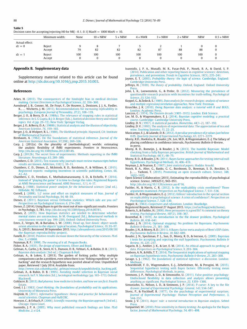
As for Bayes factors, ensuring a minimum number of trialshas occurred before stopping improves error rates for inferenceby intervals. Table 5 shows the improvement for requiring 10participants to be run before optional stopping occurs as comparedto Table 4. Still the error rates are higher than those for Bayesfactors shown in Table 2.





Accept 79 82 82 82 87 88 88 0

dz = 1 Reject 100 100 100 100 100 100 100 0Accept 0 0 0 0 0 0 0 0

Appendix B. Supplementary data

Supplementary material related to this article can be foundonline at http://dx.doi.org/10.1016/j.jmp.2015.10.003.

References

Arkes, H. (2013). The consequences of the hindsight bias in medical decisionmaking. Current Directions in Psychological Science, 22, 356–360.

Asendorpf, J. B., Conner, M., De Fruyt, F., De Houwer, J., Denissen, J. J. A., Fiedler,K., . . . Wicherts, J. M. (2013). Recommendations for increasing replicability inpsychology. European Journal of Personality, 27(2), 108–119.

Berger, J. O., & Berry, D. A. (1988a). The relevance of stopping rules in statisticalinference. In S. S. Gupta, & J. O. Berger (Eds.), Statistical decision theory and relatedtopics. Vol. 4 (pp. 29–72). New York: Springer Verlag.

Berger, J. O., & Berry, D. A. (1988b). Statistical analysis and the illusion of objectivity.American Scientist , 76, 159–165.

Berger, J. O., & Wolpert, R. L. (1988). The likelihood principle. Hayward, CA: Instituteof Mathematical Statistics.

Birnbaum, A. (1962). On the foundations of statistical inference. Journal of theAmerican Statistical Association, 57(298), 269–326.

Carp, J. (2012a). On the plurality of (methodological) worlds: estimatingthe analytic flexibility of fMRI experiments. Frontiers in Neuroscience,http://dx.doi.org/10.3389/fnins.2012.00149.

Carp, J. (2012b). The secret lives of experiments: Methods reporting in the fMRIliterature. NeuroImage, 63, 289–300.

Chambers, C. D. (2015). Ten reasons why journals must reviewmanuscripts beforeresults are known. Addiction, 110(1), 10–11.

Chambers, C. D., Dienes, Z., McIntosh, R. D., Rotshtein, P., & Willmes, K. (2015).Registered reports: realigning incentives in scientific publishing. Cortex, 66,A1–A2.

Chambers, C. D., Feredoes, E., Muthukumaraswamy, S. D., & Etchells, P. (2014).Instead of ‘‘playing the game’’ it is time to change the rules: Registered Reportsat AIMS Neuroscience and beyond. AIMS Neurosci., 1(1), 4–17.

Cohen, J. (1988). Statistical power analysis for the behavioural sciences (2nd ed.).Hillsdale, NJ: Erlbaum.

Correll, J. (2008). 1/f noise and effort on implicit measures of bias. Journal ofPersonality and Social Psychology, 94, 48–59.

Dienes, Z. (2011). Bayesian versus Orthodox statistics: Which side are you on?Perspectives on Psychological Sciences, 6, 274–290.

Dienes, Z. (2014). Using Bayes to get themost out of non-significant results. Frontiersin Psychology, 5, 781. http://dx.doi.org/10.3389/fpsyg.2014.00781.

Dienes, Z. (2015). How Bayesian statistics are needed to determine whethermental states are unconscious. In M. Overgaard (Ed.), Behavioural methods inconsciousness research (pp. 199–220). Oxford: Oxford University Press.

Estes, Z., Verges, M., & Barsalou, L. W. (2008). Head up, foot down: object wordsorient attention to the objects’ typical location. Psychological Science, 19, 93–97.

Etz, A. (2015). Retrieved 30 September 2015. http://alexanderetz.com/2015/08/30/the-Bayesian-reproducibility-project/.

Fanelli, D. (2010). Positive results increase down the hierarchy of the sciences. PLoSOne, 5, e10068.

Feynman, R. P. (1998). The meaning of it all. Penguin Books.Fisher, R. A. (1935). The design of experiments. Oliver and Boyd.Gelman, A., Carlin, J. B., Stern, H. S., Dunson, D. B., Vehtari, A., & Rubin, D. B. (2013).

Bayesian data analysis (3rd ed.). Chapman & Hall.Gelman, A., & Loken, E. (2013). The garden of forking paths: Why multiple

comparisons canbe aproblem, evenwhen there is no ‘‘fishing expedition’’ or ‘‘p-hacking’’ and the research hypothesis was posited ahead of time. Unpublishedpaper, Retrieved 1 July 2014. Available from:http://www.stat.columbia.edu/_gelman/research/unpublished/p_hacking.pdf.

Gelman, A., & Rubin, D. B. (1995). Avoiding model selection in Bayesian socialresearch. In P. V.Marsden (Ed.), Sociologicalmethodology (pp. 165–173). Oxford:Blackwell.

Goldacre, B. (2013).Bad pharma: howmedicine is broken, and howwe can fix it. FourthEstate.

Good, I. J. (1983). Good thinking: the foundations of probability and its applications.University of Minnesota Press.

Hoijtink, H. (2011). Informative hypotheses: theory and practice for behavioral andsocial scientists. Chapman and Hall/CRC.

Howson, C., & Urbach, P. (2006). Scientific reasoning: the Bayesian approach (3rd ed.).Chicago: Open Court.

Ioannidis, J. P. A. (2005). Why most published research findings are false. PLoSMedicine, 2, e124.

Ioannidis, J. P. A., Munafò, M. R., Fusar-Poli, P., Nosek, B. A., & David, S. P.(2014). Publication and other reporting biases in cognitive sciences: detection,prevalence, and prevention. Trends in Cognitive Sciences, 18(5), 235–241.

Jaynes, E. T. (2003). Probability theory: the logic of science. Cambridge, England:Cambridge University Press.

Jeffreys, H. (1939). The theory of probability. Oxford, England: Oxford UniversityPress.

John, L. K., Loewenstein, G., & Prelec, D. (2012). Measuring the prevalence ofquestionable research practices with incentives for truth-telling. PsychologicalScience, 23, 524–532.

Keppel, G., & Zedeck, S. (1989).Data analysis for research designs: analysis of varianceand multiple regression/correlation approaches. New York: Freeman.

Kruschke, J. K. (2010). Doing Bayesian data analysis: a tutorial with R and BUGS.London: Academic Press.

Lanczos, C. (1974). The Einstein decade (1905–1915). London: Elek Science.Lee, M. D., & Wagenmakers, E. J. (2014). Bayesian cognitive modeling: a practical

course. Cambridge: Cambridge University Press.Lindley, D. V. (1957). A statistical paradox. Biometrika, 44(1–2), 187–192.Lindley, D. V. (1993). The analysis of experimental data: The appreciation of tea and

wine. Teaching Statistics, 15, 22–25.Masicampo, E. J., & Lalande, D. R. (2012). A peculiar prevalence of p values just below

0.05. Quarterly Journal of Experimental Psychology, 65, 2271–2279.Morey, R.D., Hoekstra, R., Rouder, J.N., Lee, M.D., &Wagenmakers, E.-J. The fallacy of

placing confidence in confidence intervals, Psychonomic Bulletin & Review,in press.

Morey, R. D., Romeijn, J., & Rouder, J. N. (2013). The humble Bayesian: Modelchecking from a fully Bayesian perspective. British Journal of Mathematical andStatistical Psychology, 66(1), 68–75.

Morey, R. D., & Rouder, J. N. (2011). Bayes factor approaches for testing interval nullhypotheses. Psychological Methods, 16, 406–419.

Neyman, J., & Pearson, E. (1967). Joint statistical papers. Hodder Arnold.Nosek, B. A., Alter, G., Banks, G. C., Borsboom, D., Bowman, S. D., Breckler, S.

J., . . . Yarkoni, T. (2015). Promoting an open research culture. Science, 348,1422–1425.

Open Science Collaboration (2015). Estimating the reproducibility of psychologicalscience. Science, 349(6251), 943–951.http://dx.doi.org/10.1126/science.aac4716.

Pashler, H., & Harris, C. R. (2012). Is the replicability crisis overblown? Threearguments examined. Perspectives on Psychological Science, 7, 531–536.

Pashler, H., &Wagenmakers, E.-J. (2012). Editors’ introduction to the special sectionon replicability in psychological science: A crisis of confidence?. Perspectives onPsychological Science, 7, 528–530.

Popper, K. (1963). Conjectures and refutations. London: Routledge.Registered Reports, Retrieved 27 August 2015. https://osf.io/8mpji/wiki/home/.Roberts, S., & Pashler, H. (2000). Howpersuasive is a good fit? A comment on theory

testing. Psychological Review, 107(2), 358–367.Rosenthal, R. (1979). An introduction to the file drawer problem. Psychological

Bulletin, 86, 638–641.Rouder, J. N. (2014). Optional stopping: No problem for Bayesians. Psychonomic

Bulletin & Review, 21, 301–308.Rouder, J. N., &Morey, R. D. (2011). A Bayes-factormeta analysis of Bem’s ESP claim.

Psychonomic Bulletin & Review, 18, 682–689.Rouder, J. N., Speckman, P. L., Sun, D., Morey, R. D., & Iverson, G. (2009). Bayesian

t tests for accepting and rejecting the null hypothesis. Psychonomic Bulletin &Review, 16, 225–237.

Sagarin, B. J., Ambler, J. K., & Lee, E. M. (2014). An ethical approach to peeking atdata. Perspectives on Psychological Science, 9, 293–304.

Sanborn, A. N., &Hills, T. T. (2014). The frequentist implications of optional stoppingon Bayesian hypothesis tests. Psychonomic Bulletin & Review, 21, 283–300.

Savage, L. J. (1962). The foundations of statistical inference: a discussion. London:Methuen.

Schoenbrodt, F. D., Wagenmakers, E.-J., Zehetleitner, M., & Perugini, M. (2015).Sequential hypothesis testing with Bayes factors: Efficiently testing meandifferences. Psychological Methods, in press.

Simmons, J. P., Nelson, L. D., & Simonsohn, U. (2011). False-positive psychology:Undisclosed flexibility in data collection and analysis allows presentinganything as significant. Psychological Science, 22, 1359–1366.

Simonsohn, U., Nelson, L. D., & Simmons, J. P. (2014). P-curve: A key to the filedrawer. Journal of Experimental Psychology: General, 143, 534–547.

Slovic, P., & Fischhoff, B. (1977). On the psychology of experimental surprises.Journal of Experimental Psychology: Human Perception and Performance, 3,544–551.

Stone, J. V. (2013). Bayes’ rule: a tutorial introduction to Bayesian analysis. SebtelPress.

Vanpaemel, W. (2010). Prior sensitivity in theory testing: An apologia for the Bayesfactor. Journal of Mathematical Psychology, 54, 491–498.


http://refhub.elsevier.com/S0022-2496(15)00060-7/sbref1






http://dx.doi.org/10.3389/fnins.2012.00149








http://dx.doi.org/10.3389/fpsyg.2014.00781



http://alexanderetz.com/2015/08/30/the-Bayesian-reproducibility-project/











http://www.stat.columbia.edu/_gelman/research/unpublished/p_hacking.pdf






















http://dx.doi.org/10.1126/science.aac4716




https://osf.io/8mpji/wiki/home/
















Vanpaemel, W. (2014). Theory testing with the prior predictive. Oral presentationat the 26th annual convention of the association for psychological science, 22–25May, San Francisco.

Wagenmakers, E. J. (2007). A practical solution to the pervasive problems of pvalues. Psychonomic Bulletin & Review, 14, 779–804.

Wagenmakers, E. J., Wetzels, R., Borsboom, D., van der Maas, H. L. J., & Kievit,R. A. (2012). An Agenda for Purely Confirmatory Research. Perspectives onPsychological Science, 7, 632–638.

Yu, E. C., Sprenger, A. M., Thomas, R. P., & Dougherty, M. R. (2014). When decisionheuristics and science collide. Psychonomic Bulletin & Review, 21, 268–282.




how bayes factors change scientific practice...

Documents