how do equity offerings affect technology adoption...
TRANSCRIPT

0
How Do Equity Offerings Affect Technology Adoption, Employees and Firm Performance?
E. Han Kim, Heuijung Kim, Yuan Li, Yao Lu, and Xinzheng Shi†
Abstract
We hypothesize that equity offerings affect employment, wages and firm performance by facilitating technology adoption. Using regulatory shocks on the eligibility to issue seasoned equity offerings (SEOs) in China, we find that over the two-to-three years following the infusion of external capital through SEOs, firms increase expenditures on technology-related fixed- and intangible assets, and employ fewer low skill workers and more high skill workers. The decrease of low skill workers outnumbers the increase of high skill workers, resulting in a net decline in firm-level employment. Within-firm average wages increase because of the higher skill composition of employees, but total wages remain unchanged because there are fewer employees after SEOs. Finally, SEOs substantially increase firm profitability and productivity. These findings illustrate how SEOs affect employment and firm performance when financially constrained firms face an opportunity to adopt productivity-improving technologies.
March 2, 2019 Keywords: Equity Issuance, Employment, Technology Adoption, Skills, Wages, Firm Performance, Online Job Posting. JEL Classifications: G32, J21, J24, J31, L25.
†E. Han Kim is Everett E. Berg Professor of Finance at the University of Michigan, Ross School of Business, Ann Arbor, Michigan 48109: [email protected]. Heuijung Kim is an instructor at Sungkyunkwan University, SKK Business School, Seoul, Korea: [email protected]. Yuan Li is a doctoral student at University of Southern California: [email protected]. Yao Lu is Associate Professor of Finance at Tsinghua University School of Economics and Management, Beijing, China: [email protected]. Xinzheng Shi is Associate Professor of Economics at Tsinghua University School of Economics and Management, Beijing, China: [email protected]. We are grateful to Ben Iverson, Shaowei Ke, Francine Lafontaine, Binying Liu, John McConnell, Jagadeesh Sivadasan, Yifei Wang, Yinxi Xie, Stefan Zeume, and participants at various conferences and seminars for helpful comments and suggestions, and Zhang Peng and Yeqing Zhang for excellent research assistance. This project received generous financial support from Mitsui Life Financial Research Center at the University of Michigan. Yao Lu acknowledges support from Project 71722001 of National Natural Science Foundation of China. Xinzheng Shi acknowledges support from Project 71673155 of National Natural Science Foundation of China.

1
1. INTRODUCTION
News stories about automation, robots, and artificial intelligence (AI) replacing workers abound.
Under the catchy title, “Will robots displace humans as motorized vehicles ousted horses?” The
Economist (April 1, 2017) cites evidence from Acemoglu and Restrepo (2017) and warns that robots
might replace humans and depress wages. Adopting new technology, whether it involves robots, AI,
or other automation technologies, requires capital, often for large investments with uncertain
outcomes. When such investments require external funds, firms may need access to stock markets; the
newly raised equity capital, in turn, may facilitate technology adoption. Although numerous studies
examine how technology affects employment and wages (see Acemoglu and Autor (2011) for a
survey), the literature is silent on whether and how accessibility to stock markets affects technology
adoption, employment and wages, and firm performance. This paper attempts to fill the gap.
How investments financed by external capital affect employment depends on whether they
contain new technologies. If investments are purely scale expanding with no new technology—e.g.,
adding another plant using the same technology used in existing plants—firm-level employment will
increase due to the scale effect. However, some firms may deploy the external capital to adopt new
technologies automating tasks previously performed by humans, resulting in a loss of jobs—a
substitution effect. New technologies, however, may also create new tasks in which humans have
comparative advantage over machines, increasing demand for workers—a complementary effect
(Autor and Salomons, 2017; Acemoglu and Restrepo, 2018b). The net effect on firm-level
employment will then depend on how the substitution effect offsets the scale and complementary
effects.
We investigate how access to stock markets affects firm-level employment using seasoned
equity offerings (SEOs) in China. The main reason for relying on China data is identification. SEOs
are an important means to raise external capital in China, 1 and the China Securities Regulatory
1 During our sample period Chinese firms relied more heavily on the stock market for external financing than the bond market because of the relative underdevelopment of the Chinese corporate bond market (see Online Appendix 1). Our sample contains 557 public SEOs over the period 2000 through 2012. These SEOs raised over 404 billion in 2000 RMB or, on average, 726 million RMB per SEO. We do not consider initial public offerings (IPOs) because of the confounding effects of private firms becoming public firms. Bernstein (2015) argues, with supporting evidence, that IPOs change managerial incentives and/or increase managerial myopia stemming from short-term performance pressure from the stock market. Such changes may affect employment and investment

2
Commission (CSRC) issued Decree No. 30 in 2006 and No. 57 in 2008, mandating that for listed
firms to be eligible to issue public SEOs, their average payout ratios over the most recent past three
years—as defined in the regulations—must be at least 20% and 30%, respectively.2 Both regulatory
changes imposed shocks on firms that did not meet the eligibility requirements, cutting off access to
external funds through public SEOs. Note it is firms’ past actions that determine eligibility, making it
difficult for affected firms to circumvent the shocks. The shocks did not directly affect how firms use
SEO proceeds and, thus, the observed outcomes can be attributed to SEOs instead of the regulations.
To identify the causal effects of receiving SEO proceeds, we use the shocks to construct an
instrument.3 We are mindful of the issues regarding its validity. First, different payout ratios in the
past may reflect differences between the treated and untreated firms. To help satisfy the exclusion
restriction that the instrument is uncorrelated with the error term in the second-stage regressions, all
regressions control for the most recent past three-year payout ratio. Second, outcome variables of
treated and untreated firms may have different trends in the absence of the shocks. To check whether
differences in pre-trends exist for outcome variables, we use years prior to the first shock as placebo
shocks and find no difference. Third, some firms may have anticipated the regulatory changes and
circumvented them by paying higher dividends prior to the regulations than they would otherwise.
Such maneuvers, if any, are likely to manifest as a jump in payout ratios just above the thresholds
required by the regulations. We find no such discontinuity using the McCrary (2008) test. Finally, we
conduct a battery of robustness tests to the construction of our IV. The results are robust.
Our sample period is 2000 through 2012, which spans the shocks on the eligibility to issue
SEOs. During our sample period China’s labor market closely resembled those of market-oriented
economies, and its stock market became the second largest in the world in both market cap and total
value of shares traded. Online Appendix 1 reviews the literature on China’s labor market and explains
why China’s stock market is well suited to study SEOs during the sample period. Our sample contains
only listed firms because SEOs are issued by listed firms; hence, we can draw implications only at the
policies (Bertrand and Mullainathan, 2003). In addition, Agrawal and Tambe (forthcoming) report changes in employees’ skill sets when firms go through an opposite transaction—going private via leverage buyouts. 2 The payout ratio as defined in the regulations is about three times the dividend-to-earnings payout ratio. 3 We do not use the regression discontinuity (RD) design because observations around the cutoff points are too few for RD analyses. See Section 2.
3
firm level. Listed firms, however, play a major role in China’s economy. For example, in 2010, total
outputs by listed firms accounted for 43% of China’s GDP (Bryson, Forth, and Zhou, 2014).
Using the instrumental variable, we find SEOs lead to a 9.1% decline in firm-level
employment over the two-to-three years following receipts of SEO proceeds. For 557 SEOs
conducted during our sample period, the 9.1% decline implies 236,048 fewer employees remaining
with these firms, or 424 fewer employees per SEO. 4 The employment data is reliable because
disclosures of employment and payroll information in company filings and financial statements are
mandatory for listed firms in China.
How do SEOs end up reducing firm-level employment? To provide a conceptual framework
for the dynamics underlying the data, we offer a simple static model. The model relies on two
empirical regularities: (1) the primary role of equity offerings is to relax financial constraints
(DeAngelo, DeAngelo, and Stulz, 2010; and Borisov, Ellul, and Sevilir, 2017) and (2) financially
constrained firms invest less and spend less on technology (Rauh, 2006; Campello, Graham, and
Harvey, 2010). Therefore, the model assumes SEOs facilitate technology adoption by relaxing
financial constraints.5
The model then predicts that the net effect on firm-level employment depends on (1) the
productivity improvement brought about by new technology and (2) the elasticity of substitution
between high skill workers (complemented with machines) and low skill workers. When the elasticity
is greater than one and the productivity improvement is sufficiently high, machines substitute low
skill workers and complement high skill workers. Existing estimates of the elasticity of substitution
between high- and low skill workers (as classified by the level of education) is well above one, and
estimates for our sample firms also suggest an elasticity slightly above two.6 Thus, we expect SEOs
4 The decline in employment at the firm level does not imply lower employment at the economy-wide level because our sample does not include private firms and startups. Autor and Salomons (2017) argue that as aggregate productivity rises, employment at the country level, especially in the tertiary sector, tends to grow. 5 Prior studies also suggest that investments to advance technology require equity financing (e.g., Brown, Fazzari, and Petersen, 2009; Hall and Lerner, 2010; and Hsu, Tian, and Zu, 2014) 6 Existing estimates vary across time. Katz and Murphy (1992) assume that technology has a log linear increasing time trend, and obtain an estimate of 1.41 for the elasticity of substitution between college and high school graduates using US data from 1963 to 1987. Heckman, Lochner, and Taber (1998) show an estimate of 1.441 for the elasticity over 1963-1993 using a similar production function as in Katz and Murphy (1992). Extending the sample period to more recent years generates larger estimates. Card and DiNardo (2002)’s estimate of the elasticity is 1.56 when they use US data from 1967 to 1990; but when they extend the sample

4
to lead to fewer low skill workers and more high skill workers when the adoption of new technology
brings about sufficient improvement in productivity. Moreover, when the level of productivity
improvement from the new technology reaches a certain threshold, the model predicts the decline of
low skill workers will outnumber the addition of high skill workers.
To test these predictions, we rely on panel data of employee occupation and education. The
data is available because the CSRC requires publicly listed firms to disclose the composition of their
workforce by occupation and by education in yearly company filings. Our skill classification based on
occupation treats production workers and support staff as low skilled; and technicians, R&D
employees and sales and marketing forces as high skilled.7 Education-based classification treats those
with four-year university bachelor’s degrees and above as high skilled, and all others as low skilled.
Consistent with the model’s predictions, SEOs lead to a 25% reduction in production workers,
a 46% reduction in support staff, and a 17% reduction in employees without bachelor’s degrees. In
contrast, SEOs lead to a 13% increase in technicians and R&D employees, a 10% increase in sales
and marketing forces, and an 11% increase in the number of employees with post-graduate degrees.
Unconditionally, our sample firms employ more low skill workers than high skill workers;8 thus, the
net decline of total employment is due to the decrease of low skill workers outnumbering the increase
of high skill workers.
In addition, we find SEOs increase expenditures on technology-related assets, indicating more
technology adoption. The technology-related assets include fixed assets—machines and equipment—
and intangible assets—computer software, technology with or without patents, patents, and
information management systems.9 Expenditures on machinery and equipment increase by 27%, or by
period to 1999, the elasticity estimate more than doubles to 3.3. Acemoglu and Autor (2011) obtain an estimate of 2.9 for the elasticity over a sample period of 1963 to 2008, but their estimates become smaller (1.6 to 1.8) when they substitute the linear time trend with quadratic or cubic trends. As for international evidence, Card and Lemieux (2002) use UK data from 1974 to 1996 and obtain estimates of the elasticity ranging from 2 to 2.5. 7 See Section 2.4.2 for the rationale and detailed data descriptions. 8 Our sample firms employ more production workers and support staff (58% of the work force) than technicians, R&D employees, and sales and marketing forces combined (31%). (The percentages do not add up to 100 because of the omission of finance staff and others in the skill classification due to the ambiguity of their skill level.) The ratio of those without bachelor’s degrees to those with bachelor’s degrees and above is about five to one. 9 Some expenditures on machinery and equipment can be purely for replacement without any advancement in technology. However, if a sufficient portion of the expenditures on technology-related assets is used to adopt

5
40.4 million in 2000 RMB, and expenditures on intangible technology assets increase by 36%, or by
3.5 million RMB.
We are not the first to document that investments coincide with declines in firm-level
employment. Letterie, Pfann, and Polder (2004) observe that when there is an investment spike some
Dutch firms decrease employment. Hawkins, Michaels, and Oh (2015) show reductions in
employment are common among Korean plants undertaking large investments. Acemoglu and
Restrepo (2017) report a commuting zone’s exposure to robots has negative effects on employment.
The novelty of our evidence is the reduction in employment is attributable to the infusion of external
capital through SEOs that facilitates technology adoption.
The increase and decrease in the number of high and low skill workers following SEOs result
in higher skill composition of employees. The fractions of technicians and R&D employees, sales and
marketing forces, and employees with bachelor’s degrees and above increase significantly following
SEOs, while the fractions of production workers, support staff, and those without bachelor’s degrees
drop significantly. The higher skill composition, in turn, should lead to higher within-firm average
wages (total payroll/total number of employees) because higher skilled and more educated employees
are paid more (see Card, 1999; Zhang et al., 2005; and Online Appendix 7). Consistent with this
prediction, the average wage increases by 9% for all non-executive employees.
Total wages, which represent the bulk of labor costs, do not change following SEOs. Average
wages increase because of the higher skill composition, but the higher average wage applies to a
smaller number of employees due to the reduction in firm-level employment.
How do these changes in inputs of production, namely, a smaller but higher skilled workforce
using newer technology, affect firm performance? We find SEOs significantly increase profits, sales
growth, and labor and total factor productivity. Return on assets increases by 1.8 percentage points,
sales growth rate increases by 21 percentage points, annual sales per employee increases by 847,000
RMB, and total factor productivity (TFP) increases by 0.094. All these improvements are quite large
when compared to their respective sample means. The higher profits and improved productivity may
productivity-improving technology, our model predicts higher firm profitability and employee productivity, which is what we find when we examine effects of SEOs on firm performance.

6
eventually lead to greater scale and broader scope of business in the long-run, which may offset the
short-run decline in employment following SEOs.
Finally, we check whether SEOs are indeed associated with higher demand for skills by
analyzing online job advertisement data provided by a major job posting company in China. The data
are available only for 2014 - 2016, a period that does not overlap with the shocks; hence, the results
are only suggestive. We find firms receiving SEO proceeds are more likely to advertise job vacancies
requiring computer skills and non-routine analytical and interactive skills.
This paper contributes to the literature on both equity offerings and labor and finance. Prior
studies on equity offerings suggest that firms issue equity to reduce leverage (Pagano, Panetta, and
Zingales, 1998; Eckbo, Masulis, and Norli, 2000; Gustafson and Iliev, 2017), to replenish cash
balances (DeAngelo, DeAngelo, and Stulz, 2010; McLean, 2011), and to increase investments (Kim
and Weisbach, 2008; Gustafson and Iliev, 2017). We add to these contributions by providing evidence
that SEOs facilitate technology adoption and thereby affect employment and firm performance.
Perhaps most surprising, we find SEOs lead to a reduction in firm-level employment over two-to-
three years following receipts of SEO proceeds. 10 This phenomenon, however, reflects only the
immediate impacts that SEOs have on employment. The ensuing increases in firm profits and
productivity, also documented in the paper, are likely to increase the scale and scope of business,
which are likely to lead to greater employment in the long-run.
There are a number of important studies examining the effects of shocks on the accessibility
to debt or equity financing on employment.11 However, all include small and private firms, which
10Tuzel and Zhang (2018) show investment tax incentives increase high skill workers and decrease low skill workers by reducing costs of fixed investments. Their estimation of three-year effects on firm-level employment shows a negative but insignificant sign. The negative sign is consistent with our evidence that SEOs reduce firm-level employment. Investment tax credits reduce the cost of fixed-asset investments, allowing the firm to allocate more money to other input factors, which has an effect similar to increasing capital budgets. We find a more significant and stronger effect on employment, perhaps because SEOs have more direct and stronger impacts on relaxing budget constraints than investment tax credits. 11 Beck, Levine, and Levkov (2010); Benmelech, Bergman, and Seru (2011); and Carvalho (2014) study the effects of positive shocks on the accessibility to debt financing on employment in the local economy. Their identified effects are about general equilibrium results, whereas our estimates are at the firm level, which do not reflect positive externalities on the local economy. Hau and Lai (2013); Chodorow-Reich (2014); Almeida, Fos, and Kronlund (2016); Cingano, Manaresi, and Sette (2016); Acharya, Eisert, Eufinger, and Hirsch (2018); and Bentolila, Jansen, and Jimenez (2018) study the effects of negative shocks on the accessibility to debt or equity financing on firm-level employment. Their identified effects are not comparable to ours, because frictions in reversing investment and employment decisions, such as adjustment costs and sticky production processes,

7
may use their externally raised capital for purposes quite different from those of publicly-listed firms.
More important, none of the prior studies considers how the shocks on the accessibility to external
financing affect technology adoption. By exploring the technology channel, we add to the literature (1)
new evidence on the differential impacts that SEOs have on the employment of high- vs. low skill
workers and (2) how SEOs improve firm performance when financially constrained firms have
opportunities to adopt productivity-improving technologies. In so doing, we provide insights into two
important issues largely ignored by the finance literature: how SEOs affect employees and
productivity.
We also add to the debate on how financial leverage affects wages. A number of prior studies
argue a decrease in financial leverage increases wages by weakening employers’ bargaining position
against employees, whereas others argue the same decrease in financial leverage decreases wages by
reducing ex-ante employment risk.12 Empirical studies on this issue rely on average wages, which we
show depends on the skill composition of employees. Firms with low financial leverage tend to be
less financially constrained (Giroud and Mueller, 2017), which may allow more investments in
technology and human capital, leading to a higher skill composition and a higher average wage.
Employee skill composition, therefore, seems an important omitted variable in the debate over how
leverage affects wages.
Finally, this paper contributes to the literature on the capital-technology-skill
complementarity. Identification of the complementarity is difficult because of endogeneity issues.
Lewis (2011) and Akerman, Gaarder, and Mogstad (2015) provide cleaner identification using
exogenous shocks, but their findings apply only to the technology-skill complementarity, without
linking financial capital (as opposed to physical capital) to technology or skills. We show how
infusion of financial capital via SEOs facilitates technology adoption and affects employment, skill
make the effects of negative shocks asymmetrical to those of positive cash inflows from SEOs. Although our IV is constructed using negative shocks on the eligibility to issue SEOs, our IV estimation results reflect the effects of receiving SEO proceeds. As such, our results do not apply to firms having to cut budgets. Bai, Carvalho, and Phillips (2018) study how positive shocks on accessing debt capital affect the growth rate of employment differently between younger and older, more productive and less productive firms. 12 See Matsa (2018) for a more in-depth summary of the debate. Studies suggesting a negative relation include Bronars and Deer (1991); Perotti and Spier (1993); and Michaels, Page, and Whited (forthcoming). Studies suggesting a positive relation include Berk, Stanton, and Zechner (2010) and Chemmanur, Cheng, and Zhang (2013).

8
composition, wages, and firm performance. Acemoglu and Finkelstein (2008) is more closely related;
they find a decrease in the price of capital relative to labor for hospitals leads to more adoption of new
health care technology, decreases total labor input, and upgrades the skill composition of hospital
nurses. We add to their contribution by expanding the scope of investigation. We show the capital
skill complementary process triggered by SEOs also affects wages and improves firm productivity.
We also demonstrate that capital-technology-skill complementarity applies well beyond the hospital
sector and nurses; it holds for a broad range of sectors and occupations.
The next section describes our empirical strategy and data; Section 3 provides evidence on
how SEOs affect firm-level employment; Section 4 provides a theoretical framework to help interpret
the data; Section 5 presents evidence on technology adoption, wages, and firm performance; Section 6
conducts robustness tests; Section 7 examines online job advertisements; and Section 8 concludes.
2. EMPIRICAL STRATEGY AND DATA
We employ an IV approach using shocks on the eligibility to issue SEOs. It provides direct
estimates of the impacts that SEOs have on outcome variables. We do not use a difference-in-
differences (DID) approach because it provides estimates of the effects of regulatory changes instead
of the effects of SEOs.13 Nor do we use a regression discontinuity design because observations in the
neighborhood around the 20% and 30% thresholds in 2006 and 2008 shocks are too few to conduct
meaningful RD analyses.14
2.1. Regulatory Changes on the Eligibility to Issue SEOs
On May 6, 2006, the CSRC issued Decree No.30 requiring that to conduct a public SEO, a
firm’s cumulative distributed profits in cash or stocks during the most recent past three years must be
13 Let y = α + β ∗ SEO + ε, where β captures effects of SEOs. We construct an IV from a regulatory shock, and the relation between SEO and IV is SEO = γ + δ ∗ IV + v . The DID approach estimates y = α + β ∗(γ + δ ∗ IV + v) + ε = α + β ∗ γ + β ∗ δ ∗ IV + β ∗ v + ε . That is, the coefficient we get from the DID approach is β ∗ δ, not β that we hope to estimate using the IV approach. 14 For the 2006 regulation cutoff, there are no eligible firms conducting SEOs and four ineligible firms not conducting SEOs in the neighborhood of [19%, 21%]. For wider neighborhoods of [17%, 23%] and [15%, 25%], there are one and four eligible firms conducting SEOs and 7 and 11 ineligible firms not conducting SEOs, respectively. For the 2008 regulation cutoff, for the neighborhoods of [29%, 31%], [27%, 33%], and [25%, 35%], the number of eligible firms conducting SEOs is 2, 11, and 22; the number of ineligible firms not conducting SEOs is 7, 13, and 22. For the neighborhood containing the most observations ([25%, 35%]), the calculated power of the RD strategy for the estimated effect of SEOs on total employment by the IV strategy in the paper (i.e., the coefficient of SEO� in Table 3, Column 1) is only 0.060, substantially lower than the conventional threshold 0.8. Stata code "rdpower" is used for this calculation.

9
no less than 20% of the average annual distributable profits realized over the same period. 15 Prior to
this regulation, the eligibility requirement was a positive dividend during the past three years. The
catalyst for the regulation was the Split Share Structure Reform of 2005, which made non-tradable
controlling shares tradable in stock markets beginning 2005. The Reform led to a large increase in the
supply of tradable shares, which the CSRC deemed adversely influenced stock price. Preventing low
payout firms from issuing new shares was supposed to dampen new supply of tradable shares.
The CSRC further tightened the requirement when it issued Decree No.57, which raised the
threshold to 30%, counting only cash payments as distributed profits. This regulation was triggered by
a stock market crash. The Shanghai Stock Exchange Composite Index reached its peak on October 16,
2007, then fell precipitously, dropping more than 50% by June 2008. The CSRC raised the bar in
order to prevent further decline in stock prices by reducing the supply of newly issued shares. It
issued a draft of the 2008 regulation on August 22, 2008, followed by an official announcement on
October 9, 2008.
The CSRC specifies the formula for the payout ratio as (Dt-1 + Dt-2 + Dt-3) / [(It-1 + It-2+ It-3) / 3],
where Dt is the amount of dividends paid in year t and It is the amount of distributable profits in year t
as measured by net income (the parent’s net income for consolidated financial statements,
http://www.csrc.gov.cn/zjhpublic/zjh/200804/t20080418_14487.htm.). 16 Dt includes stock dividends
when calculating the ratio for the 2006 regulation, but only cash dividends when calculating the 2008
regulation ratio. Because of the way the formula defines the denominator, the payout ratio is roughly
three times the average annual payout ratio over the past three years.
2.2. The SEO Variable and Its Instrument
2.2.1. The SEO Variable
We follow prior studies on equity offerings (e.g., Kim and Weisbach, 2008; DeAngelo et al.,
2010) and define the SEO variable, SEO, as the “SEO years” in which proceeds from SEOs are most 15 The regulators tied the eligibility to issue SEOs to past dividend payouts because they believed firms paying out more free cash flows are less likely to waste them and better serve investors. Go to http://www.csrc.gov.cn/pub/newsite/hdjl/zxft/lsonlyft/200710/t20071021_95210.html for a press conference on the 2006 regulation. For more details, see Regulation for Issuing Stocks, 2006, China’s Securities Regulatory Commission. 16Also, see http://www.csrc.gov.cn/pub/newsite/gszqjgb/fwzn/201603/t20160329_294910.html. For firms listed for less than three years, the same formula (with fewer years) applies to the years they have been listed (see the CSRC internal publication, BaoJianYeWuTongXun (Investment Banking Practice Letters) 2, 2010, p.24).
10
likely to affect outcome variables of interest. Some firms receive SEO proceeds very late in the year
and it takes time for the capital infusion to affect employment, investments, and firm performance;
therefore, we define SEO as the year of receiving SEO proceeds and two years afterward.
2.2.2. Construction of the Instrument
The instrument for SEO, SEOIneligible, is an indicator of whether the regulations prevented a
firm from receiving SEO proceeds during the SEO years. Consider the 2006 regulation. Firms are
treated by this regulation if their average payout ratios over 2003 – 2005 are less than 20%. Note that
starting an SEO process in 2006 may not provide the firm with the proceeds in 2006. In our sample,
the average time elapsed from the initial SEO announcement to the receipt of the proceeds is 337
calendar days. So if a firm received SEO proceeds in 2006, it is likely that the SEO was approved
before the 2006 regulation took effect. Therefore, we use a two-year lag to match the SEO variable
SEO with the applicable instrumentation: if the 2006 regulation treated a firm in 2006, we assume it
prevented the firm from receiving SEO proceeds in 2008, and turn on SEOIneligible in 2008, 2009,
and 2010. (We use a two-year lag because the shocks occurred in May 2006 and October 2008. The
results are robust to using a one-year lag.) We also allow the 2006 regulation to treat firms in 2007
because it may be difficult to circumvent the regulation in 2007 by increasing dividends in 2006 alone.
So if a firm has less than 20% payout ratio over 2004 – 2006, we turn on the instrument in 2009, 2010,
and 2011. Results are robust to turning off the instrument for firms affected by the 2006 regulation in
2007 (See Section 6.2.)
We follow the same procedure for firms treated by the 2008 regulation. SEOIneligible is
equal to one in 2010, 2011, and 2012 for firms with average payout ratios less than 30% over 2005 –
2007, and in 2011 and 2012 for firms with average payout ratios less than 30% over 2006 – 2008.
Online Appendix 2 illustrates the construction of the instrument.
2.2.3. Validity of the Instrument
The exclusion restriction condition requires the instrument to be uncorrelated with the error
terms in the second stage. Two potential issues could affect the validity of our instrument. First,
treated and untreated firms may differ to the extent that past dividend payouts reflect firm
characteristics. For example, firms may pay out more of their earnings when management anticipates

11
positive shocks to cash flows in the future. As the anticipated positive shocks realize, firms make
more investments in technology, leading to changes in outcome variables of interest. For this reason,
all regressions control for the most recent past three-year payout ratio, P3_PR, which determines the
variation in treatment. We also examine, in Section 6.1, whether treated and untreated firms would
have had different time trends in outcome variables had there been no shock. Placebo tests using data
prior to the regulations indicate no different pre-trends in outcome variables between treated firms and
untreated firms prior to the first shock in 2006.
Second, if some firms circumvented the regulations by increasing payout ratios prior to the
shocks, firms in greater need of external capital for investments are more likely to manipulate the
payout ratios. Such maneuvers are difficult and costly. Otherwise low-payout firms will have to
anticipate the regulatory changes. The anticipation is subject to uncertainty, reducing the present value
of benefits from the maneuvers. The uncertainty is not only about future regulations; there is also the
uncertainty of approval. SEOs require the CSRC’s approval, which adds uncertainty over whether and
how much capital an SEO can raise. The cost of maneuvering dividends in anticipation of the 2008
regulation is likely to be economically significant because it counts only cash dividends. 17
Maneuvering dividend payouts in anticipation of the 2006 regulation can be less costly because it
counts stock dividends as payouts. If low-payout firms anticipated this aspect of the forthcoming
regulation, they could have satisfied the dividend requirement by issuing sufficient stock dividends
during 2003 - 2005. Data show otherwise. Stock dividends were relatively rare in China during that
period. Among 600 dividend cases in 2005, for example, only 41 included stock dividends. Over the
2003-2005 period, 94% of all the dividend cases did not include any stock dividends.
If, in spite of these considerations, some firms somehow manipulated payout ratios to meet
the eligibility requirements, the average payout ratios for the most recent past three years are likely to
be just above 20% in 2006 and 30% in 2008. They are unlikely to exceed the thresholds by much
because the maneuvers would force the firm to payout more than it would otherwise. To check
17 To circumvent the 2008 regulation, a firm would have to guess the higher required payout ratio, pay more dividends than it would otherwise, then gross up the size of the SEO to make up for the difference. Such maneuvers are costly due to financing frictions. Firms wishing to issue SEOs tend to be cash constrained (DeAngelo et al., 2010); paying out extra cash would exacerbate the constraint, forcing the firm to forego value-enhancing investments.

12
whether there are discontinuities in the most recent past three-year payout ratios at 20% for 2006 and
at 30% for 2008, we use the method proposed in McCrary (2008). Using Stata command “DCdensity,”
which chooses bin size and bandwidth, yields a discontinuity estimate of 0.724 for 2006, with
standard error and P-value of 0.708 and 0.306, respectively. For 2008, the discontinuity estimate is
0.179, with standard error and P-value of 0.274 and 0.514. Although the McCrary test is only about
the necessary condition, the results support the validity of our instrument.
2.3. Baseline Specification
All regressions control for year- and firm fixed effects. Year fixed effects control for
economy-wide shocks, such as labor policy changes or stock market crashes, while firm fixed effects
control for time-invariant firm characteristics. As noted, all regressions control for the most recent
past three-year payout ratio, P3_PR. Some firm-years show negative P3_PR because some firms with
negative average annual distributable profit over the past three years paid dividends when they had a
profitable year over the same period. We avoid losing these observations by replacing a negative
P3_PR by one.18 We distinguish those observations by adding a dummy, P3_PR_D for a negative
ratio. In addition, we control for the following time-varying variables.
Legal Variables: (1) The minimum wage required in the province or provincial-level city of a firm’s
headquarters location, Ln(MIN_WAGE). Minimum wages, which are adjusted every two or three
years, may affect not only employment but also the skill composition of employees by imposing a
lower limit on what firms can pay unskilled workers. (2) Effects of the Labor Law of People’s
Republic of China on employment and wages. The law, which became effective on January 1, 2008,
has greater effects on firms with higher labor intensity. We measure the law’s effect,
Labor_Law_Effect, by the interaction of the labor intensity, as measured by the industry average ratio
of the total number of employees to total fixed assets in 2007, with a post-regulation indicator equal to
one for 2008 through 2012. We use industry classifications as defined by the CSRC. (3) Local legal
environment, LAWSCORE. A higher score indicates the firm is located in a region with more
developed legal institutions and stronger law enforcement. We include this variable because the law
18 We assign one to negative P3_PR because the dividend payout ratio in the year a firm pays dividends while having negative average profits over the three-year period is likely to be very high. None of our sample firms paid dividends when they reported a loss.
13
and finance literature suggests firms located in countries with stronger investor protection tend to
have stronger corporate governance and suffer from fewer agency problems, which may affect firms’
investment decisions and labor policies.19
Firm Characteristics: (1) Firm age, the log of the number of years a firm has been listed,
Ln(NYEAR_LISTED). (2) Firm size, the log of sales, Ln(SALES). (3) The percentage of shares held by
local or central government, %_STATE_OWN. State share ownership varies substantially over time
and across firms. (4) The current dividend payout ratio, DIV_PR. Higher dividends may reduce the
misuse of free cash flows (Jensen, 1986), influencing the outcome variables of interest. Since
dividends are serially correlated, current dividends may be related to the past dividend payouts used to
construct the instrument. (5) Strength of corporate governance. Strong governance reduces misuse of
SEO proceeds (Jung, Kim, and Stulz, 1996; Kim and Purnanandam, 2014), influencing investments,
employment and wages (Jensen, 1986; Bertrand and Mullainathan, 2003; Atanassov and Kim, 2009;
Cronqvist et al., 2009; Kim and Ouimet, 2014). Proxies for governance include the aforementioned
LAWSCORE; ownership concentration, the percentage of shares held by the largest
shareholder, %_LARGST_SH; board independence, the percentage of independent directors on the
board, %_IND_DIR. (6) Asset tangibility, property, plants, and equipment over total assets, PPE/TA.
High-tech firms tend to have fewer fixed assets and fewer production workers. (7) Financial leverage,
Leverage, to partial out the leverage channel through which SEOs may affect our key outcome
variables. SEOs reduce leverage (Pagano, Panetta, and Zingales, 1998; Eckbo, et al., 2000; Gustafson
and Iliev, 2017), and as mentioned earlier, a number of studies argue leverage affects employment and
wages. (8) Percentage of non-tradable shares, %_NONTRD_SH, to control for the potential
confounding effects of the Split Share Structure Reform.
2.4. Data and Summary Statistics
2.4.1. Sample Construction and Data Sources
The sample period covers 2000 through 2012 to span the regulatory shocks. China first
allowed underwritten offerings in 2000, and data for many key variables are available only after 2000.
19 The National Economic Research Institute (NERI) constructs the index for each province or provincial-level region. The index changes, reflecting changes in the number of lawyers as a percentage of the population, the efficiency of the local courts, and the protection of property rights (Wang, Wong, and Xia, 2008).
14
The sample includes all A-share firms listed on the Shanghai and Shenzhen Stock Exchanges.20 We
exclude financial firms as defined by the CSRC (e.g., banks, insurance firms, and brokerage firms);
firms with fewer than 100 employees; and ST (special treatment) and *ST firms, which have had two
(ST) or three (*ST) consecutive years of negative net profit.
Table 1 lists the sample distribution by year. The sample contains 17,838 firm-year
observations associated with 2,341 unique firms. In total, our sample contains 557 public SEOs. We
do not include privately placed equity offerings because the 2006 and 2008 shocks do not apply to
private offerings. The table shows a surge of public SEOs when underwritten offerings were first
allowed in 2000. The small number of SEOs in 2005 and 2006 is due to the suspension of all public
equity offerings during the Split Share Structure Reform. (The suspension began in April 2005 and
ended in May 2006.) SEO activities recovered in 2007 and increased in 2008, but the aforementioned
stock market crash and the 2008 regulation appear to have dampened SEOs; their number dropped in
2009 and remained low until the end of the sample period.
The primary source of data for labor, financial, and corporate governance variables is Resset
(http://www.resset.cn/en/). Although similar to Compustat, Resset provides reliable data on wages and
employment that we can link to our sample firms. The data is reliable because disclosures of
employment and payroll information in company filings and financial statements are mandatory for
listed firms in China. For data on SEOs and expenditures on technology-related assets, we rely on
CSMAR (http://www.gtarsc.com/). We hand collect minimum wages from provincial government
webpages. Online Appendix 3 lists the data source for each variable.
2.4.2. Skill Variables
Acemoglu and Autor (2011: p. 1045) define skills as “a worker’s endowment of capabilities
for performing various tasks,” where a task is defined as “a unit of work activity that produces output.”
The labor literature classifies tasks into three broad categories: abstract, routine, and manual (Autor,
Katz, and Kearney, 2006; Autor and Dorn, 2013). Abstract tasks, such as research and legal writing,
tend to require high skills. Routine tasks, such as picking/sorting, repetitive assembling, and record
20 Stock markets in China offer two types of stocks: A- and B shares. We restrict our sample to the A-share market because the total market capitalization of the A-share market is about 122 times that of the B-share market as of the end of 2013 and most firms listed in the B-share market are also listed in the A-share market.

15
keeping, are codifiable manual and cognitive tasks following explicit procedures, which tend to
require low skills. Non-routine manual tasks, such as janitorial service and driving, are tasks requiring
physical adaptability, which also tend to require low skills (Autor and Handel, 2013).
We proxy the level of skills by occupation and education. Each occupation may comprise
multiple tasks at different levels of intensity, but the variation is greater across occupations than
within an occupation (Autor and Handel, 2013). The intensity of routine tasks is greater in
occupations such as production workers, assemblers, and support staff than occupations such as
engineers, R&D staff, and sales and marketing forces. Thus, we classify production workers and
support staff as low skill workers and engineers, R&D staff, and sales and marketing forces as high
skill workers. We also use education as a proxy for skill, and classify employees with at least
bachelor’s degrees from four-year universities and above as high skill workers and the rest as low
skill workers.
The CSRC requires publicly listed firms to disclose in yearly company filings the
composition of their workforce by occupation and by education. Although it does not require a
specific format, all firms report the number of employees by occupation or job type, and most firms
report the number of employees by education. Resset collects the information and constructs firm-
level panel data on the number of employees by occupation and education. It also provides written
descriptions of each job type coded from the company filings for each firm-year.
We manually clean the occupation data by cross-checking with textual descriptions in the
filings. Firms vary in defining occupations due to differences in the nature of business, operation, and
organizational structure. Consequently, occupation data in Resset show some inconsistencies between
occupation variable names and textual descriptions of occupation or job type. We also find some jobs
classified as “others” by Resset classifiable into a specific occupation group using the written
descriptions.
We define six occupation-based categories. The first, Production, is production workers. It
includes mainly blue-collar workers performing assembly line work, sorting, moving, and other
routine physical tasks. Most firms report this category quite clearly. Some high-tech and non-
manufacturing firms do not have employees in this category.
16
The second, Staff, stands for support staff. This category is not as clear-cut as the production
worker category. Some firms report the number of employees with a finer breakdown, such as office
support staff and HR staff, while others aggregate them into one category of staff. Support staff may
include both office staff (receptionists, secretaries, customer service providers, and office
administrators) and non-office staff (employees for warehouse maintenance, security, and logistics
support, including their supervisors). Some firms report office and non-office staff separately, while
others lump them together. To make the data comparable across firms, we manually check written
descriptions for each firm-year and aggregate the number of employees in all staff positions. The
majority of employees in this group perform routine clerical or non-routine low-skill manual tasks.
However, this group also includes managerial positions (e.g., HR manager, logistics supervisor, office
managers), which require non-routine abstract skills.
The third, Tech_R&D, includes technicians and R&D staff. Technicians include engineers
and IT staff, who tend to possess technical skills for non-routine tasks. R&D staff include scientists,
researchers, and designers working on creative tasks and development of new products. We group
technicians and R&D staff into one category because only about 20% of our sample firms have a
separate category for R&D employees.
The fourth, S&M, is the sales and marketing force, which includes sales persons and
employees in marketing, advertising, and brand management. Most of these employees perform non-
routine tasks requiring communication and analytical skills.
The fifth, Finance, includes record keepers, accountants, and financial managers for capital
budgeting, investment, and asset management. Record keepers and low-level accountants perform
routine tasks, while high-level accountants and finance staff tend to perform non-routine abstract tasks.
We cannot tell whether the majority in this category perform routine or non-routine abstract tasks.
The last category, Others, includes those reported as “others” by sample firms and job
categories that cannot be put into one of the above categories, such as “operating”. Some firms put
sales force in the same group with technicians or with financial accountants. Since we cannot separate
them, we treat them as Others. We do the same when some firms report the number of managers. We

17
do not make a separate category for managers because only about 25% of sample firms report the
number of managers, which cannot mean the rest of sample firms do not have managers.
To separate employees by education, we construct three education groups: holders of post-
graduate degrees, Grad; holders of four-year university bachelor’s degrees and above, BA; and those
with no four-year university bachelor’s degree, NBA. Grad includes all master’s and doctorate degrees
(e.g., MS, MA, MBA, EMBA, PhD, MD, and JD). About 50% of sample firms separately report the
number of employees with post-graduate degrees, while others lump those with four-year university
bachelor’s degree and post-graduate degree into one category. To make data comparable across firms,
when firms separately report post-graduate degree and four-year university bachelor’s degree holders,
we combine them to construct BA. When firms report degree holders from three-year or lower level
colleges and degree holders from four-year universities as one group, we do not include them in BA.
2.4.3. Descriptive Statistics
Table 2 provides the summary statistics for all key variables. Online Appendix 3 provides
variable definitions. To mitigate outlier problems, we winsorize all financial variables at the 1% and
99% level and replace them with the value at 1% or 99%. We normalize all monetary variables to year
2000 RMB.
The indicator for SEO years, SEO, shows that 9% of firm-year observations are in SEO years.
The instrument, SEOIneligible, indicates that the regulatory shocks treated 16% of observations. The
average fractions of production workers, support staff, technicians and R&D staff, sales and
marketing forces, finance staff, and others are 48%, 9%, 18%, 13%, 3%, and 17%, respectively.21 The
very high percentage of production workers reflects the fact that China was the manufacturing hub of
the world during the sample period and the exclusion of the financial services sector. The average
number of employees is 4,592, and about 20% of employees have bachelor’s degrees and above, and
3% have post-graduate degrees.22 The average past three-year payout ratio, P3_PR, is about three
21 The percentages do not sum to 100% because of missing observations. 22 The sum of mean BA and mean NBA is greater than the mean EMP, the total number of employees. This is because many small firms do not separately report the number of employees with four-year university bachelor’s degrees and above, often lumping them together with those with junior college and vocational school degrees. As mentioned earlier, we do not include those small firms when we calculate the number of employees with BA or NBA. When we calculate the mean EMP, we include all firms in the sample

18
times the average annual dividend payout ratio, DIV_PR,23 because of the unique way P3_PR is
defined. (See the formula in Section 2.1.) The average wage for all employees, AWAGE, is slightly
lower than the average wage for all non-executive employees, AWAGE_NonExe, because AWAGE is
calculated over 2000-2012, while AWAGE_NonExe is over 2001-2012 (firms did not separately
disclose payroll information for executives until 2001).
3. EMPLOYMENT AND EMPLOYEE SKILL COMPOSITION
We begin our investigation by estimating how SEOs affect firm-level employment and the
composition of employees by occupation or education.
3.1. Firm-level Employment
We rely on the two-stage IV estimation for identification. The first stage is estimated by the
firm-level conditional (fixed-effects) logistic regression because the endogenous variable SEO is an
indicator. Under the assumption that the instrument has predictive power over the endogenous
variable, IV estimators using the logit model in the first stage are asymptotically efficient; i.e.,
coefficients of the model can be more precisely estimated (Wooldridge, 2010, p. 939). Standard errors
of the first-stage regression are clustered at the firm level, and those of the second-stage regression are
corrected by bootstrapping. Online Appendix 4, Column (1) reports the first-stage result. The
coefficient on SEOIneligible is negative and highly significant, indicating that the instrument has
strong predictive power over SEO. F-statistics are not reported because the regression is conditional
logit, a non-linear estimation. The F-statistic is 14.06 when the first-stage is estimated using the OLS.
Table 3 reports the second-stage results for employment level. The first column shows a 9.1%
decline in total employment. Over the sample period of 13 years, there were 557 SEOs (see Table 1).
The total number of people employed by these firms at the time of issuing SEOs was 2,593,934. Thus,
the 9.1% decline implies 236,048 fewer employees remain with these firms following SEOs, or 424
fewer employees per SEO. Coefficients on control variables are consistent with intuition. There are
more employees when firms are older and larger, and have a greater state share of ownership, more
tangible assets, and higher leverage. Firms located in regions with higher minimum wage and stronger
legal environments tend to have fewer employees.
23 The minimum DIV_PR is zero because no firm in our sample paid dividends in a year of negative profits.

19
We do not rely on the OLS estimate because of bias due to unobservable time-varying factors
correlated with employment and SEOs. For example, steady employment growth to maintain social
stability is a high priority of the Chinese government.24 Since the central government internalizes all
the external effects of social stability (Bai, Lu, and Tao, 2006), the CSRC might be more inclined to
approve an SEO if the applying firm has a large workforce and needs to raise money to keep them
employed. Without accounting for this unobservable factor, OLS estimates of how SEOs affect
employment will contain an upward bias. For the record, we report the OLS estimate with the baseline
specification in the first column of Online Appendix 5, Column (1), which indicates SEOs are
associated with a 3% decline in total employment, a smaller decline than the IV estimate.
3.2. Composition of Employee Occupation and Education
The remaining columns in Table 3 break down employees by occupation or education, where
the dependent variable is the log of one plus the number of employees (some firm-years show no
employees in some occupation and education categories.) The number of technicians and R&D
employees, the sales and marketing force, and post-graduate degree holders increases by 13%, 10%,
and 11%, respectively. 25 In contrast, the number of production workers, support staff, and employees
without four-year university bachelor’s degree decreases by 25%, 46%, and 17%, respectively.
Because there are more employees in the latter group than in the former group, these results imply
SEOs lead to more displacement of low skill workers than to adding high skill workers.
The changes in the level of high- and low skill workers should lead to a higher skill
composition of employees. That is what we find in Table 4, which reports second-stage results for
occupation- and education composition. SEOs significantly increase the fractions of technicians and
R&D employees, the sales and marketing force, and finance staff. The fractions of employees with
four-year university bachelor’s degrees and above and with post-graduate degrees also significantly
24 Premier Wen Jiabao states in the 2010 Government Work Report, “the government promises to do everything in our power to increase employment” (Wen, Jiabao, 2010 年 政 府 工 作 报 告http://www.gov.cn/2010lh/content_1555767.htm.) 25 When Grad is the dependent variable, the number of observations falls sharply because only about 50% of sample firms separately report the number of employees with post-graduate degrees.

20
increase. In contrast, SEOs significantly decrease the fractions of production workers, support staff,
and employees without four-year university bachelor’s degree.26
4. THEORETICAL FRAMEWORK
The net decline in firm-level employment following SEOs is surprising because one normally
associates the infusion of capital with an increase in the scale of operation necessitating more
employees. In a typical Cobb-Douglas production function of labor and capital, for example, relaxing
the budget constraint would increase the optimal levels of both. However, the data indicate that the
decline in employment is due to the decrease of low skill workers outnumbering the increase of high
skill workers. To provide a conceptual framework to interpret this finding, we offer a simple static
model wherein relaxing financial constraints by issuing SEOs stimulates new technology adoption.
4.1. A Simple Model
We consider the optimal choice of production inputs for a profit-maximizing firm. The firm
can continue to operate with the technology that it currently owns, or alter its production process by
adopting a new technology. The firm’s current cash balance, K, which is given, can only pay for the
inputs of production using the old technology. The cash balance is insufficient to pay for the new
technology, so adopting the new technology requires raising external capital ∆K through an SEO. We
compare the optimal inputs of production before and after the SEO.
We follow Acemoglu and Autor (2010) and assume the production of final goods is a constant
elasticity of substitution (CES) aggregation of two intermediate inputs. One intermediate input is
produced by H high skill workers with A machines, using a Cobb-Douglas production function,
𝜀𝜀𝜀𝜀𝛼𝛼𝐻𝐻1−𝛼𝛼 , where 𝜀𝜀 denotes the productivity of high skill workers with machines and 𝛼𝛼 measures the
share of machines in the production. The production of the other intermediate input only uses L low
skill workers. Therefore, the production function of final goods takes the form of �(𝜀𝜀𝜀𝜀𝛼𝛼𝐻𝐻1−𝛼𝛼)𝜎𝜎−1σ +
𝐿𝐿𝜎𝜎−1σ �
𝜎𝜎𝜎𝜎−1
, where 𝜎𝜎 is the elasticity of substitution between the two intermediate inputs. This production
26 Table 4 does not report the estimation result on the fraction of NBA, because %_NBA is equal to 1 - %_BA; hence, the coefficients on %_NBA are the same as those on %_BA with the signs reversed.

21
function has constant returns to scale, which make the optimal scale undetermined. However, in our
model the scale is bounded by budget constraints, which we assume are exogenous.
Note that the production function does not assume Hicks-neutral technological progress.
Instead, we follow Kahn and Lim (1998) and Acemoglu (2002) and assume each production input
factor experiences its own specific technological progress. That is, skilled labor-augmenting
technological progress improves the productivity of high skill workers much more than that of low
skill workers. Advancement of computer software is an example; its impact on the productivity of
high skill workers is much greater than that of low skill workers. For simplicity, we assume the
productivity of low skill workers remain constant at one when technological advances improve high
skill workers’ productivity.
Payments for the inputs of production are made at the beginning of the period, subject to a
budget constraint K. Production outputs generate revenue at the end of the period. The firm is a price
taker for both inputs and outputs. The cost of using a machine is r, the wage of a high skill worker is
w, and the wage of a low skill worker is 1; and w > 1 because of the skill premium. The present value
of the future revenue is, p, the present value of price per unit of output, times outputs. With these
assumptions, the firm’s profit maximization problem with the old technology before an SEO is:
𝑉𝑉(𝐾𝐾, 𝜀𝜀) ≡ 𝑀𝑀𝑀𝑀𝑀𝑀{𝐴𝐴,𝐻𝐻,𝐿𝐿}
𝑝𝑝 �(𝜀𝜀𝜀𝜀𝛼𝛼𝐻𝐻1−𝛼𝛼)𝜎𝜎−1σ + 𝐿𝐿
𝜎𝜎−1σ �
𝜎𝜎𝜎𝜎−1
− 𝑟𝑟𝜀𝜀 − 𝑤𝑤𝐻𝐻 − 𝐿𝐿
s. t. 𝑟𝑟𝜀𝜀 + 𝑤𝑤𝐻𝐻 + 𝐿𝐿 = 𝐾𝐾
The profit maximization problem changes if the firm adopts the new technology. This part of
the model borrows heavily from Midrigan and Xu (2014): Technology adoption increases the capital-
augmenting productivity by 𝜙𝜙 ≥ 0 such that the productivity of high-skilled production becomes 𝜀𝜀 +
𝜙𝜙. Adopting the technology requires one-time investment in sunk cost, 𝐶𝐶(𝜙𝜙), at the beginning of the
period. The cost is higher when the productivity improvement is greater . Both 𝜙𝜙 and 𝐶𝐶(𝜙𝜙) are
exogenous and the firm’s choice is binary—it either adopts the new technology or does not. The firm
is financially constrained due to financing frictions and needs to issue an SEO to raise ∆𝐾𝐾 ≥
𝐶𝐶(𝜙𝜙), where ∆𝐾𝐾 is the sum of net SEO proceeds and incremental debt supported by the new equity
capital. If the firm adopts the new technology after the SEO, its profit maximization problem becomes:

22
𝑉𝑉(𝐾𝐾 + ∆𝐾𝐾 − 𝐶𝐶(𝜙𝜙), 𝜀𝜀 + 𝜙𝜙) ≡ 𝑀𝑀𝑀𝑀𝑀𝑀{𝐴𝐴,𝐻𝐻,𝐿𝐿}
𝑝𝑝 ��(𝜀𝜀 + 𝜙𝜙)𝜀𝜀𝛼𝛼𝐻𝐻1−𝛼𝛼�𝜎𝜎−1σ + 𝐿𝐿
𝜎𝜎−1σ �
𝜎𝜎𝜎𝜎−1
− 𝑟𝑟𝜀𝜀 − 𝑤𝑤𝐻𝐻 − 𝐿𝐿
s. t. 𝑟𝑟𝜀𝜀 + 𝑤𝑤𝐻𝐻 + 𝐿𝐿 = 𝐾𝐾 + ∆𝐾𝐾 − 𝐶𝐶(𝜙𝜙)
Appendix A provides solutions to both profit maximization problems. We denote the optimal
level of machines, high skill workers, and low skill workers before an SEO as 𝜀𝜀1∗ , 𝐻𝐻1∗, and 𝐿𝐿1∗ ,
respectively. If the firm upgrades its technology after the SEO, these optimal levels change to 𝜀𝜀2∗ , 𝐻𝐻2∗,
and 𝐿𝐿2∗ . Let 𝑚𝑚 = �1−𝛼𝛼𝑤𝑤�1−𝛼𝛼
�𝛼𝛼𝑟𝑟�𝛼𝛼
, then the optimal level of inputs are:
𝜀𝜀1∗ = 𝛼𝛼𝛼𝛼𝑟𝑟�1 − 1
1+[𝑚𝑚𝑚𝑚]𝜎𝜎−1� (1)
𝐻𝐻1∗ = (1−𝛼𝛼)𝛼𝛼𝑤𝑤
�1 − 11+[𝑚𝑚𝑚𝑚]𝜎𝜎−1� (2)
𝐿𝐿1∗ = 𝛼𝛼
1+[𝑚𝑚𝑚𝑚]𝜎𝜎−1 (3)
𝜀𝜀2∗ = 𝛼𝛼𝑟𝑟�𝐾𝐾 + ∆𝐾𝐾 − 𝐶𝐶(𝜙𝜙)� �1 − 1
1+[𝑚𝑚(𝑚𝑚+𝜙𝜙)]𝜎𝜎−1� (4)
𝐻𝐻2∗ = 1−𝛼𝛼𝑤𝑤�𝐾𝐾 + ∆𝐾𝐾 − 𝐶𝐶(𝜙𝜙)� �1 − 1
1+[𝑚𝑚(𝑚𝑚+𝜙𝜙)]𝜎𝜎−1� (5)
𝐿𝐿2∗ = 𝛼𝛼+∆𝛼𝛼−𝐶𝐶(𝜙𝜙)1+[𝑚𝑚(𝑚𝑚+𝜙𝜙)]𝜎𝜎−1 (6)
Lemma. Infusion of external capital through an SEO can increase profits regardless of whether the
capital is deployed to upgrade the technology. But if 𝐾𝐾 + ∆𝐾𝐾 > 𝐾𝐾∗, where 𝐾𝐾∗ ≡
𝐶𝐶(𝜙𝜙)�𝑝𝑝��𝑚𝑚(𝑚𝑚+𝜙𝜙)�𝜎𝜎−1+1�
1𝜎𝜎−1−1�
𝑝𝑝���𝑚𝑚(𝑚𝑚+𝜙𝜙)�𝜎𝜎−1+1�
1𝜎𝜎−1−[(𝑚𝑚𝑚𝑚)𝜎𝜎−1+1]
1𝜎𝜎−1�
, the increase in profits will be greater if the firm upgrades its
technology than if it simply expands the scale of operation with the old technology.
Proof: See Appendix A
The Lemma establishes that if a firm can raise sufficient funds such that 𝐾𝐾 + ∆𝐾𝐾 > 𝐾𝐾∗ , it will
upgrade its technology. The threshold point, 𝐾𝐾∗, is the capital level at which the firm is indifferent
between upgrading its technology and keeping the old technology. When 𝐾𝐾 + ∆𝐾𝐾 > 𝐾𝐾∗, the
productivity improvement with the new technology is worth more than the cost of adopting the

23
technology, leading to a higher profit than the profit the firm can achieve by expanding the scale of
operation using the old technology.
Proposition. If a firm upgrades technology after an SEO and 𝜎𝜎 > 1, 𝜀𝜀2∗ > 𝜀𝜀1∗ and 𝐻𝐻2∗ > 𝐻𝐻1∗. And if
𝜙𝜙 ∈ [0,𝐶𝐶−1(∆𝐾𝐾)], there exists a 𝜙𝜙�, such that when 𝜙𝜙 > 𝜙𝜙� , 𝐿𝐿1∗ > 𝐿𝐿2∗ . Furthermore, there also exists a
𝜙𝜙∗ > 𝜙𝜙�, such that when 𝜙𝜙 > 𝜙𝜙∗, 𝐻𝐻1∗ + 𝐿𝐿1∗ > 𝐻𝐻2∗ + 𝐿𝐿2∗ .
Proof: See Appendix A.
The Proposition specifies the conditions under which the number of low skill workers and total
employment decline following an SEO. Specifically, 𝜎𝜎 > 1 means that the high skill production and
low skill production are substitutes. Note that 𝐿𝐿1∗
𝐿𝐿2∗= 𝛼𝛼
𝛼𝛼+∆𝛼𝛼−𝐶𝐶(𝜙𝜙)1+[𝑚𝑚(𝑚𝑚+𝜙𝜙)]𝜎𝜎−1
1+(𝑚𝑚𝑚𝑚)𝜎𝜎−1 . The first component
𝛼𝛼𝛼𝛼+∆𝛼𝛼−𝐶𝐶(𝜙𝜙) can be interpreted as the scale effect on low skill workers, that is, if the external capital
raised through an SEO exceeds the cost of technology upgrade, this component increases 𝐿𝐿2∗ relative
to 𝐿𝐿1∗ . The second component 1+[𝑚𝑚(𝑚𝑚+𝜙𝜙)]𝜎𝜎−1
1+(𝑚𝑚𝑚𝑚)𝜎𝜎−1 can be interpreted as the substitution effect; with an
increase in the productivity of high skill production, low skill production will be replaced if they are
substitutes (𝜎𝜎 > 1). If the productivity of high skill production increases sufficiently such that 𝜙𝜙 > 𝜙𝜙�,
then the substitution effect dominates the scale effect, resulting in 𝐿𝐿1∗
𝐿𝐿2∗ > 1. That is, the number of low
skill workers declines after the SEO. Furthermore, if the increase in productivity of high skill
production is so high that 𝜙𝜙 exceeds 𝜙𝜙∗ > 𝜙𝜙�, the decline of low skill workers will outnumber the
increase of high skilled workers, leading to a reduction in total number of employees.27
4.2. Within-firm Average Wages, Profitability and Employee Productivity
The proposition provides additional predictions. Within-firm average wage is:
𝜀𝜀𝐴𝐴𝐴𝐴𝑟𝑟𝑀𝑀𝐴𝐴𝐴𝐴 𝑤𝑤𝑀𝑀𝐴𝐴𝐴𝐴 = 𝑇𝑇𝑇𝑇𝑇𝑇𝑇𝑇𝑇𝑇 𝑤𝑤𝑇𝑇𝑤𝑤𝑤𝑤𝑇𝑇𝑇𝑇𝑇𝑇𝑇𝑇𝑇𝑇 𝑛𝑛𝑛𝑛𝑚𝑚𝑛𝑛𝑤𝑤𝑟𝑟 𝑇𝑇𝑜𝑜 𝑤𝑤𝑇𝑇𝑟𝑟𝑤𝑤𝑤𝑤𝑟𝑟𝑤𝑤
= 𝑤𝑤𝐻𝐻∗+𝐿𝐿∗
𝐻𝐻∗+𝐿𝐿∗= 1 + 𝑤𝑤−1
1+𝐿𝐿∗𝐻𝐻∗
(7)
When 𝜙𝜙 > 𝜙𝜙�, 𝐿𝐿∗ declines while 𝐻𝐻∗ increases after an SEO; hence, 1 + 𝐿𝐿∗
𝐻𝐻∗ decreases and the average
wage increases.
27 Note that the proposition specifies an upper bound 𝐶𝐶−1(∆𝐾𝐾) for 𝜙𝜙. This condition excludes situations where ∆𝐾𝐾 is so large that the scale effect dominates all other effects.

24
The total firm profit before an SEO can be obtained by plugging 𝜀𝜀∗, 𝐻𝐻∗ and 𝐿𝐿∗ into the profit
function:
𝑉𝑉(𝐾𝐾, 𝜀𝜀) = 𝑝𝑝 ��𝜀𝜀𝜀𝜀∗𝛼𝛼𝐻𝐻∗1−𝛼𝛼�𝜎𝜎−1σ + 𝐿𝐿∗
𝜎𝜎−1σ �
𝜎𝜎σ−1
− 𝑟𝑟𝜀𝜀∗ − 𝑤𝑤𝐻𝐻∗ − 𝐿𝐿∗
= 𝑝𝑝𝐾𝐾[(𝑚𝑚𝜀𝜀)𝜎𝜎−1 + 1]1
𝜎𝜎−1 − 𝐾𝐾
Defining the profitability as the total profit divided by the total expenditures on inputs, we obtain
𝑃𝑃𝑟𝑟𝑃𝑃𝑓𝑓𝑖𝑖𝑖𝑖𝑀𝑀𝑖𝑖𝑖𝑖𝑖𝑖𝑖𝑖𝑖𝑖𝑖𝑖 = 𝑉𝑉(𝛼𝛼,𝑚𝑚)𝛼𝛼
= 𝑝𝑝[(𝑚𝑚𝜀𝜀)𝜎𝜎−1 + 1]1
𝜎𝜎−1 − 1.
Because 𝜀𝜀 increases to 𝜀𝜀 + 𝜙𝜙 after the SEO, profitability will increase if 𝜎𝜎 > 1.
We define employee productivity by output per worker. Since the total output before an SEO
is 𝑝𝑝𝐾𝐾[(𝑚𝑚𝜀𝜀)𝜎𝜎−1 + 1]1
𝜎𝜎−1,
𝑂𝑂𝑂𝑂𝑖𝑖𝑝𝑝𝑂𝑂𝑖𝑖 𝑝𝑝𝐴𝐴𝑟𝑟 𝑤𝑤𝑃𝑃𝑟𝑟𝑤𝑤𝐴𝐴𝑟𝑟 = 𝑝𝑝𝛼𝛼�(𝑚𝑚𝑚𝑚)𝜎𝜎−1+1�1
𝜎𝜎−1
𝐻𝐻∗+𝐿𝐿∗.
The Proposition shows that if 𝜙𝜙 > 𝜙𝜙∗, total employment 𝐻𝐻∗ + 𝐿𝐿∗ decreases after the SEO, while 𝜀𝜀
increases to 𝜀𝜀 + 𝜙𝜙; therefore, output per worker will increase after the SEO.
4.3. Elasticity of Substitution
A critical condition required for the above predictions is that the elasticity of substitution
between machine-augmented high skill tasks and low skill tasks is greater than one. All existing
estimates of the elasticity of substitution between high- and low skill workers based on U.S. and U.K.
data are well above one (see footnote 7 in Introduction.) To check whether the condition is also
satisfied for our sample firms, we estimate the elasticity in Appendix B. We employ two
specifications, linear and non-linear time trends for technology development. We also use two
classifications for high- and low skill workers, one education based, and the other occupation based.
Elasticity estimates based on education are about 2.1, which is within the range of existing estimates
based on education. Our elasticity estimates based on occupation are about 4.8, which are also
comparable to existing estimates based on occupation.28
28 Card (2001) reports that the implied estimate of the elasticity of substitution between occupations ranges from 5 to 10, which is much larger than the estimates based on education.

25
5. TECHNOLOGY ADOPTION, WAGES, AND FIRM PERFORMANCE
5.1. Technology Adoption
Our model assumes that relaxing financial constraints via SEOs facilitates technology
adoption. We test this assumption using expenditures on technology-related fixed- and intangible
assets. The fixed assets are machines and equipment. The intangible assets are computer software,
technology with or without patents, patents, and information management systems. We exclude
intangible assets not directly related to technology, such as goodwill, rights to land use, and
franchising. Data on expenditures for machines and equipment are available from 2003 when the
CSRC first required listed firms to breakdown fixed assets by type. Data on intangible assets are
available only from 2007 because the CSRC did not require the breakdown of intangible assets by
type until 2007. The CSMAR is the data source.
Table 5 reports the second-stage estimation results. The estimated coefficient in the first
column implies that SEOs increase expenditures on machines and equipment by 27%, or by 40.2
million 2000 RMB (.27 x 148.9M in Table 2). The estimated coefficient in the second column implies
that SEOs increase expenditures on technology-related intangible assets by 36%, or by 3.5 million
2000 RMB (0.36 x 9.8M in Table 2).29
Given the nature of technology-related intangible assets, it is reasonable to assume that most
expenditure on the intangible assets involve either new technology or an updated version of
technology currently in use. The same can be said about expenditures on machines and equipment;
however, some can be purely for replacement purpose without any advancement in technology. If a
sufficient portion of the expenditures on technology-related assets in our sample is made to adopt
productivity-improving technologies, our model predicts firm profitability and employee productivity
will both improve following SEOs. We test this prediction in the next section.
The third column of Table 5 confirms previous findings that SEOs increase capital
expenditures (e.g., Kim and Weisbach, 2008; Gustafson and Iliev, 2017). Because capital
29 The second column does not contain LAWSCORE as a control variable because it does not have variation over the sample period for the intangible assets: the data for the intangible assets begins in 2007 and the National Economic Research Institute updates LAWSCORE only up to 2009.

26
expenditures include investments unrelated to technology, we cannot draw inferences on technology
adoption from this result; however, it illustrates that our sample firms are not unique.
5.2. Firm Performance
To test the effects of SEOs on firm performance, we measure profitability by return on assets,
ROA. For productivity, we use three different, yet related, measures: sales growth, SALES_GR for
output growth rate; sales per employee, SALES/Employees for worker productivity; and total factor
productivity, TFP.
Table 6 reports the second-stage estimation results. SEOs significantly improve all four
measures of performance. The magnitude of improvement in each measure is substantial in
comparison to the sample mean. ROA increases by 1.8 percentage points (sample mean = 3.5%).
Sales growth rate increases by 21 percentage points (sample mean = 23%). Sales per employee
increases by 847,000 RMB (sample mean = 1,105,000 RMB). TFP increases by 0.094 (sample mean
= 0.003.) 30
5.3. Wages
The higher skill composition following SEOs will increase within-firm average wages
because of the skill premium. The China Urban Household Survey shows that Chinese workers with
more education are paid more, and technicians are paid substantially more than production, staff and
service, or agricultural workers (see Online Appendix 7). Table 7 reports the second-stage results,
which show significantly higher average wages following SEOs. The last two columns separate
employees into non-executive employees and executives. Non-executive employees, whose average
wage increases by 9%, drive the increase in average wages. Average wages of executives (classified
30 We recognize our TFP estimates may contain biases. The TFP in the table is the residual of an OLS estimation of the production function, which regresses the log of total output value on the log of total assets and the log of total number of employees. We include firm- and year fixed effects to control for any time-invariant firm-specific shocks and economy wide time-specific shocks. Nevertheless, the estimates could be biased due to the correlations between input levels and unobservable time-varying firm-specific shocks. Levinsohn and Petrin (2003) suggest using intermediate inputs to control for the correlation between input levels and unobservable time-varying firm-specific shocks; however, data on intermediate inputs are not available for our sample firms. As a robustness check, we re-estimate the production function by replacing the total number of employees with the total number of production workers and with the total payroll. The results, reported in Online Appendix 6, are robust. However, these alternative measures of TFP may still be biased.

27
as such in financial statements) do not increase significantly, suggesting that the effect of SEOs on
executive skill composition is immaterial.31
Coefficients on control variables are largely consistent with intuition. Average wages are
positively related to minimum wage, firm size, past payout ratio, state share ownership, ownership
concentration, and intangibility of assets, and are negatively related to leverage.
How do changes in employment and skill composition affect total wages? Because the total
number of employees declines, the higher average wage does not necessarily imply a higher total
wage. Table 8 reports the second-stage results for total wages. SEOs have no significant impact on
total wages regardless of how we stratify employee groups.
6. ROBUSTNESS TESTS
In this section, we examine pre-trends prior to the first shock and test whether our evidence is
robust to alternative ways to construct the instrument and to excluding small SEOs.
6.1. Pre-Trends
The instrument is based on the variation in the impacts that regulatory shocks have on firms’
eligibility to issue SEOs. Its validity requires that if there were no shock, affected and unaffected
firms would not show different time trends in the outcome variables. As a way to test the parallel
trend assumption, we conduct a placebo test using the 2000-2005 sample prior to the 2006 shock. We
do not use the post-2006 shock sample for two reasons: (1) the presence of the second shock in 2008
and (2) the composition of treated and untreated firms changes from year to year starting in 2007
because the variable determining the treatment, P3_PR, is a moving average over the past three years.
We construct an indicator for firms affected by the 2006 regulation, Affected. Then we test
whether there is any difference between the outcome varables of shock-affected and shock-unaffected
31 The executive wage results do not reflect the value of equity incentives, which are an important component of executive compensation in the U.S. In China, wages constitute most of executive compensation, with executive stock options playing no, or a minor, role in the compensation during our sample period. Bryson et al. (2014) reports, “Fewer than 1% of top executives were granted options in any given year between 2006 and 2010 and, for these few cases, at the median they were worth 30% of CEO cash compensation and 21% of non-CEO top executive cash compensation.” Chinese firms were unable to offer stock options until 2006, when equity incentives were formally introduced in the form of employee stock options and discounted share purchase programs. Stock options are granted and vested shortly after shareholder approval. They are exercisable according to a fixed schedule tied to certain performance targets. Discounted share purchase programs allow stock purchases at a discount but they cannot be sold until a performance target is achieved. These equity incentives are issued to both non-executive employees and executives.

28
firms during the years prior to 2006 using 2000 as the base year. We define five placebo shock
indicators, Year01,…, Year05, which equal to one in 2001,…, 2005, respectively. We then estimate
the baseline regression for all key outcome variables with the interactions of Affected and placebo
indicators.
Table 9 reports the coefficients on the interaction terms, which are insignificant for all but one
at the ten percent level, suggesting no different time trends in the outcome variables between affected
and unaffected firms prior to the 2006 shock.32
6.2. Alternative Ways to Construct the Instrument and Definition of the SEO Variable
Since the instrument is the key to our identification, we test the robustness of our results to
three alternative ways to construct the instrument. First, some firms may circumvent the 2006 and
2008 regulations in 2007 and 2009, respectively, by increasing dividends in 2006 and 2008. To guard
against such possibilities, we turn on the instrument only for firms treated by the 2006 regulation in
2006 and firms treated by the 2008 regulation in 2008. Second, we shorten the time elapsed from the
beginning of the SEO process to the receipt of proceeds from two years to one year. Third, we rely
only on the 2006 shock because some firms may have anticipated the 2008 shock. In addition, we
exclude small SEOs in the bottom decile for proceeds. Firms conducting these small SEOs are
typically small cap firms with highly volatile performance. Table 10 reports the second-stage results
for all outcome variables. All results are robust. Online Appendix 4, Columns (2) – (5) report the first-
stage estimation results.
7. DEMAND FOR SKILLS
We explain the decline in firm-level employment by invoking capital skill complementarity
and using occupation and education as proxies for skills. As a final check on the underlying
presumption that SEOs increase the demand for skills, we use job-posting data to measure the demand
for computer and non-routine task skills. We then relate the demand for these skills to SEOs. The data
is obtained from a major job posting company in China, Lagou.com (https://www.lagou.com). It
32 Placebo shock indicators for expenditures on machinery and equipment cover only 2004 and 2005 with 2003 as the base year because data on purchases of machines and equipment are available only from 2003. We cannot conduct the placebo test on technology-related intangible assets because the data are available only from 2007, a year after the 2006 shock.

29
started the job posting business in 2013, so our data covers only 2014 through 2016, which does not
overlap with the regulatory shocks. As such, the results presented here are only suggestive, as we
relate endogenous variables without exogenous variation. Nevertheless, they serve as a robustness test,
because if we find no relation between SEOs and demand for skill, it will cast doubt on the validity of
our explanation for the decline in firm-level employment.
The job posting sample contains 45,585 unique full-time job advertisements by 790 A-share
firms listed on Shanghai and Shenzhen Stock Exchanges over 2014 – 2016. We exclude repetition of
the same advertisements that firms re-post to attract more attention. Online Appendix 8, Panel A
shows that of 45,585 new job postings, 7,791 are from firms receiving SEO proceeds. Because the
estimation in this section does not rely on the shocks to the eligibility to issue public SEOs, we
include both public and private placements.
Our approach to construct skill variables is similar to Hershbein and Kahn (2018). For each
job advertisement, we machine-search for the keywords indicating four types of skills: (1) advanced
computer skills, (2) basic computer skills, (3) non-routine analytical task skills, and (4) non-routine
interactive task skills. Online Appendix 8, Panel B lists the English translation of Chinese keywords
used to identify each skill.
All estimations are at the job advertisement level, relating skills mentioned in each job
posting to whether the posting occurred during the year in which a company receives SEO proceeds.33
The dependent variable is either an indicator for the presence of a keyword indicating a specific skill
or the log of one plus the number of key words associated with each skill type to capture the intensity
of the skill requirement. The variable of interest is the SEO indicator, JP_SEO, which equals to one
only in the year of receiving SEO proceeds.34 All regressions control for year- and firm dummies to
control for heterogeneity in demand for skills and jobs across time and firm. We also control for
location dummies at the county level because many firms operate in multiple locations and job skill
requirements vary across different locations (R&D centers requiring advanced computer and non-
33 We cannot conduct firm level analyses because firms may advertise job openings with other job posting companies and/or through other recruiting channels. 34 We turn on the indicator only in the year a firm receives SEO proceeds because the sample period covers only three years. If a firm fills newly-advertised positions in the year of the posting, the advertisement is unlikely to appear in the following year unless the newly hired employees leave the firm.
30
routine analytical skills tend to be located in metropolitan areas, while sales offices tend to be located
in both countryside and metropolitan areas.)
Table 11, Panel A reports the results relating advanced computer skills to the SEO indicator.
Columns (1) and (3) show positive and significant coefficients, which suggest firms receiving SEO
proceeds are more likely to specify advanced computer skills in their job posting.35 Hershbein and
Kahn (2018) point out online job postings tend to target white-collar employees more than blue-collar
workers. To control for job-related omitted variables, we add job dummies in Columns (2) and (4)
using job titles mentioned in the postings. Reestimation results continue to show significant positive
coefficients on the SEO indicator, suggesting that when firms receive SEO proceeds, their demand for
advanced computer skills increase even for the same type of jobs. Panel B repeats the same exercise
for basic computer skills. Coefficients on the SEO indicator are again positive and significant;
indicating the likelihood of specifying basic computer skills in job advertisements is higher when
firms receive SEO proceeds.
In Table 12, we relate the SEO indicator to non-routine analytical and interactive task skills.
Again, the coefficients are all positive and six of the eight coefficients are significant. In sum, firms
obtaining new capital through SEOs exhibit greater demand for computer and non-routine task skills.
8. SUMMARY AND IMPLICATIONS
This paper investigates how capital infusion through SEOs affects technology adoption, firm-
level employment, employee skill composition, wages, and firm performance. To identify causal
effects, we rely on external shocks that cut off access to public SEOs as a means to raise external
capital. We find SEOs facilitate adoption of productivity-improving technologies, and displace more
low skill workers than adding high skill workers, leading to lower firm-level employment. The higher
skill composition following SEOs increases within-firm average wages because of the skill premium,
but total wages remain unchanged because of the reduction in total employment. Thus, SEOs allow
firms to upgrade technology and upgrade employee skills without increasing the total wage bill. These
changes in the inputs to production result in higher profits, greater output, and improvement in worker
and total factor productivity. These findings demonstrate the impacts that SEOs can have on
35 We lose three observations for OLS regressions because location information is unavailable.

31
employees and firm performance when financially constrained firms have opportunities to adopt
productivity-improving technologies.
Our findings also shed light on how accessibility to stock markets affects labor markets by
altering the demand for high- vs. low skill workers. Easier access to capital may not only increase
demand for high skill workers but also stimulate their supply, since the demand for and the supply of
skills is endogenous to each other and dynamically moves together. If the supply of high skill workers
increases in response to increased demand, it may induce greater development of skill complementary
technologies, which is likely to enhance economic growth.
The highly developed, sophisticated, global financial markets of recent years have allowed
easier access to external capital, which our evidence suggests can lead to displacement of low skilled
and less-educated workers. Unless there are other employers absorbing displaced low skill workers
with equivalent jobs, demand for their skills will decline. Retraining to upgrade skills requires
financial resources, time, and effort; thus, many low skill workers may not be able to leave the
shrinking market for their services, at least not in the short run. The ensuing imbalance between the
supply of and the demand for low skilled and less-educated workers is likely to keep their income low.
High skilled and more-educated employees, on the other hand, will enjoy increasing demand for their
services as frictions to accessing external capital decline and capital skill complementarity kicks in.
The result might be further widening income inequality in the short-run.
In the end, however, the improvement in firm performance and productivity resulting from
better access to capital will enlarge the scale of the economy, offsetting the declining demand for low
skill workers. In addition, the positive spillovers of technology advances to the tertiary sector might
offset the negative employment effect on low skill workers (Autor and Salomons, 2017). When low
skill workers undergo proper retraining to perform tasks needed for the larger economy and tertiary
services, the aggregate employment opportunities might grow as capital markets facilitate
development of complementary technologies and processes to harness the recent technological
advances to yield their full economic benefits.

32
APPENDIX A: Equations (1) through (6) and Proofs of the Lemma and the Proposition
Derivations of Equations (1) through (6) in Section 4.1.
The firm faces an output price, p, and a series of input prices; r is the rent to use a machine, w is the
wage of a high skill worker. The wage of a low skill worker is 1 such that other prices are relative to
the low skill worker wage. Because of the skill premium, w > 1. K is the budget to pay for the usage
of machines and for the employment of high- and low skill workers. The production function is of a
simple CES form, �(𝜀𝜀𝜀𝜀𝛼𝛼𝐻𝐻1−𝛼𝛼)𝜎𝜎−1σ + 𝐿𝐿
𝜎𝜎−1σ �
𝜎𝜎𝜎𝜎−1
, 𝜎𝜎 ∈ [0,∞). It is similar to the production function in
Autor, Katz, and Krueger (1998), except we allow the technology to augment only high skill workers.
The profit maximization problem faced by the firm before an SEO is:
𝑀𝑀𝑀𝑀𝑀𝑀{𝐴𝐴,𝐻𝐻,𝐿𝐿}
𝑝𝑝 �(𝜀𝜀𝜀𝜀𝛼𝛼𝐻𝐻1−𝛼𝛼)𝜎𝜎−1σ + 𝐿𝐿
𝜎𝜎−1σ �
𝜎𝜎𝜎𝜎−1
− 𝑟𝑟𝜀𝜀 −𝑤𝑤𝐻𝐻 − 𝐿𝐿
s. t. 𝑟𝑟𝜀𝜀 +𝑤𝑤𝐻𝐻 + 𝐿𝐿 = 𝐾𝐾 (A1)
The Lagrangian function for solving (A1) is
𝐿𝐿(𝜀𝜀,𝐻𝐻, 𝐿𝐿, 𝜆𝜆) = 𝑝𝑝 �(𝜀𝜀𝜀𝜀𝛼𝛼𝐻𝐻1−𝛼𝛼)𝜎𝜎−1σ + 𝐿𝐿
𝜎𝜎−1σ �
𝜎𝜎𝜎𝜎−1
− 𝑟𝑟𝜀𝜀 − 𝑤𝑤𝐻𝐻 − 𝐿𝐿 + 𝜆𝜆(𝐾𝐾 − 𝑟𝑟𝜀𝜀 − 𝑤𝑤𝐻𝐻 − 𝐿𝐿).
Let 𝑀𝑀 = (𝜀𝜀𝜀𝜀𝛼𝛼𝐻𝐻1−𝛼𝛼)𝜎𝜎−1σ + 𝐿𝐿
𝜎𝜎−1σ . Then, the first-order necessary conditions for this maximization
problem are as follows:
𝐿𝐿𝐴𝐴 = 𝑝𝑝𝑀𝑀𝜎𝜎
𝜎𝜎−1−1𝛼𝛼𝜀𝜀𝜎𝜎−1σ 𝜀𝜀𝛼𝛼
𝜎𝜎−1σ −1𝐻𝐻(1−𝛼𝛼)𝜎𝜎−1
σ − (1 + 𝜆𝜆)𝑟𝑟 = 0 (A2)
𝐿𝐿𝐻𝐻 = 𝑝𝑝𝑀𝑀𝜎𝜎
𝜎𝜎−1−1(1− 𝛼𝛼)𝜀𝜀𝜎𝜎−1σ 𝜀𝜀𝛼𝛼
𝜎𝜎−1σ 𝐻𝐻(1−𝛼𝛼)𝜎𝜎−1
σ −1 − (1 + 𝜆𝜆)𝑤𝑤 = 0 (A3)
𝐿𝐿𝐿𝐿 = 𝑝𝑝𝑀𝑀𝜎𝜎
𝜎𝜎−1−1𝐿𝐿𝜎𝜎−1σ −1 − (1 + 𝜆𝜆) = 0 (A4)
𝐿𝐿𝜆𝜆 = −𝑟𝑟𝜀𝜀 − 𝑤𝑤𝐻𝐻 − 𝐿𝐿 + 𝐾𝐾 = 0 (A5)
Combining equations (A2) and (A3) yields
𝛼𝛼𝐻𝐻(1−𝛼𝛼)𝐴𝐴
= 𝑟𝑟𝑤𝑤
(A6)
Combining equations (A2) and (A4) yields
𝛼𝛼𝑚𝑚𝜎𝜎−1σ 𝐴𝐴𝛼𝛼
𝜎𝜎−1σ −1𝐻𝐻(1−𝛼𝛼)𝜎𝜎−1
σ
𝐿𝐿𝜎𝜎−1σ −1
= 𝑟𝑟 (A7)

33
Combining equations (A5), (A6) and (A7) and defining 𝑚𝑚 = �1−𝛼𝛼𝑤𝑤 �
1−𝛼𝛼�𝛼𝛼𝑟𝑟�
𝛼𝛼, we derive the optimal
choice of machines, high skill workers, and low skill workers before an SEO as:
𝜀𝜀1∗ = 𝛼𝛼𝛼𝛼𝑟𝑟�1 − 1
1+[𝑚𝑚𝑚𝑚]𝜎𝜎−1�
𝐻𝐻1∗ = (1−𝛼𝛼)𝛼𝛼𝑤𝑤
�1 − 11+[𝑚𝑚𝑚𝑚]𝜎𝜎−1�
𝐿𝐿1∗ = 𝛼𝛼
1+[𝑚𝑚𝑚𝑚]𝜎𝜎−1
Following the same procedure, we derive the optimal choice of machines, high skill workers, and low
skill workers if the firm upgrades technology after an SEO:
𝜀𝜀2∗ = 𝛼𝛼𝑟𝑟�𝐾𝐾 + ∆𝐾𝐾 − 𝐶𝐶(𝜙𝜙)� �1 − 1
1+[𝑚𝑚(𝑚𝑚+𝜙𝜙)]𝜎𝜎−1�
𝐻𝐻2∗ = 1−𝛼𝛼𝑤𝑤�𝐾𝐾 + ∆𝐾𝐾 − 𝐶𝐶(𝜙𝜙)� �1 − 1
1+[𝑚𝑚(𝑚𝑚+𝜙𝜙)]𝜎𝜎−1�
𝐿𝐿2∗ = 𝛼𝛼+∆𝛼𝛼−𝐶𝐶(𝜙𝜙)1+[𝑚𝑚(𝑚𝑚+𝜙𝜙)]𝜎𝜎−1
Proof of Lemma
The firm’s maximum profit is:
𝜋𝜋0 = 𝑝𝑝𝐾𝐾 �[(𝑚𝑚𝜀𝜀)𝜎𝜎−1 + 1]1
𝜎𝜎−1 − 1�, with the old technology and a budget of 𝐾𝐾.
𝜋𝜋1 = 𝑝𝑝(𝐾𝐾 + ∆𝐾𝐾) �[(𝑚𝑚𝜀𝜀)𝜎𝜎−1 + 1]1
𝜎𝜎−1 − 1�, with the old technology and a budget of 𝐾𝐾 + ∆𝐾𝐾.
𝜋𝜋2 = 𝑝𝑝�𝐾𝐾 + ∆𝐾𝐾 − 𝐶𝐶(𝜙𝜙)�{�(𝑚𝑚(𝜀𝜀 + 𝜙𝜙))𝜎𝜎−1 + 1]1
𝜎𝜎−1 − 1�, with the new technology and a budget of
𝐾𝐾 + ∆𝐾𝐾.
It is easy to see that 𝜋𝜋1𝜋𝜋0
> 1 and 𝜋𝜋2𝜋𝜋0
> 1. Therefore, profits are higher with the infusion of capital
through an SEO regardless of whether the firm upgrades the technology.
The firm will upgrade the technology if 𝜋𝜋2 > 𝜋𝜋1; that is, if
𝜋𝜋2 − 𝜋𝜋1 = 𝑝𝑝(𝐾𝐾 + ∆𝐾𝐾)([(𝑚𝑚(𝜀𝜀 + 𝜙𝜙))𝜎𝜎−1 + 1]1
𝜎𝜎−1 − [(𝑚𝑚𝜀𝜀)𝜎𝜎−1 + 1]1
𝜎𝜎−1)
− 𝐶𝐶(𝜙𝜙) �𝑝𝑝[(𝑚𝑚(𝜀𝜀 + 𝜙𝜙))𝜎𝜎−1 + 1]1
𝜎𝜎−1 − 1� ≥ 0

34
Writing 𝜋𝜋2 − 𝜋𝜋1 as a function of 𝐾𝐾 + ∆𝐾𝐾, or 𝑓𝑓(𝐾𝐾 + ∆𝐾𝐾), it follows that 𝑓𝑓 increases monotonically
with 𝐾𝐾 + ∆𝐾𝐾. Thus, we derive 𝐾𝐾∗ that satisfies 𝑓𝑓(𝐾𝐾∗) = 0
𝑓𝑓(𝐾𝐾∗) = 0 ⇒ 𝐾𝐾∗ =𝐶𝐶(𝜙𝜙) �𝑝𝑝[(𝑚𝑚(𝜀𝜀 + 𝜙𝜙))𝜎𝜎−1 + 1]
1𝜎𝜎−1 − 1�
𝑝𝑝([(𝑚𝑚(𝜀𝜀 + 𝜙𝜙))𝜎𝜎−1 + 1]1
𝜎𝜎−1 − [(𝑚𝑚𝜀𝜀)𝜎𝜎−1 + 1]1
𝜎𝜎−1)
Therefore, if 𝐾𝐾 + ∆𝐾𝐾 > 𝐾𝐾∗, the firm will upgrade its technology to maximize its profit.
Rewriting 𝐾𝐾∗= 𝐶𝐶(𝜙𝜙)�𝑝𝑝[�𝑚𝑚(𝑚𝑚+𝜙𝜙))𝜎𝜎−1+1�
1𝜎𝜎−1−1�
𝑝𝑝(([(𝑚𝑚(𝑚𝑚+𝜙𝜙))𝜎𝜎−1+1]1
𝜎𝜎−1−1)−([(𝑚𝑚𝑚𝑚)𝜎𝜎−1+1]1
𝜎𝜎−1−1)) and rearranging, we obtain:
�𝐾𝐾∗ − 𝐶𝐶(𝜙𝜙)� �𝑝𝑝[(𝑚𝑚(𝜀𝜀 + 𝜙𝜙))𝜎𝜎−1 + 1]1
𝜎𝜎−1 − 1� = 𝐾𝐾∗ �𝑝𝑝 �[(𝑚𝑚𝜀𝜀)𝜎𝜎−1 + 1]1
𝜎𝜎−1 − 1��.
That is, 𝑉𝑉(𝐾𝐾∗ − 𝐶𝐶(𝜙𝜙), 𝜀𝜀 + 𝜙𝜙) = 𝑉𝑉(𝐾𝐾∗, 𝜀𝜀) . Since 𝑉𝑉(𝐾𝐾∗ − 𝐶𝐶(𝜙𝜙), 𝜀𝜀 + 𝜙𝜙) is the profit with the
technology upgrade and 𝑉𝑉(𝐾𝐾∗, 𝜀𝜀) is the profit without the technology upgrade,𝐾𝐾∗ is the capital level
at which the firm is indifferent between upgrading its technology and keeping the old technology.
Proof of Proposition.
First, we prove that if 𝜎𝜎 > 1, then 𝜀𝜀2∗ > 𝜀𝜀1∗ and 𝐻𝐻2∗ > 𝐻𝐻1∗. The intuition is the scale effect. Because
∆𝐾𝐾 ≥ 𝐶𝐶(𝜙𝜙), 𝐾𝐾 + ∆𝐾𝐾 − 𝐶𝐶(𝜙𝜙) ≥ 𝐾𝐾. Further, because 𝜙𝜙 ≥ 0, 𝜀𝜀 + 𝜙𝜙 ≥ 𝜀𝜀. And if 𝜎𝜎 > 1, we can easily
check from the above optimal solutions that 𝜀𝜀2∗ > 𝜀𝜀1∗ and 𝐻𝐻2∗ > 𝐻𝐻1∗.
To compare 𝐿𝐿1∗ with 𝐿𝐿2∗ , we define 𝑓𝑓(𝜙𝜙) = 𝐿𝐿1∗
𝐿𝐿2∗ = 𝐾𝐾
𝐾𝐾+∆𝐾𝐾−𝐶𝐶(𝜙𝜙)1+[𝑚𝑚(𝜀𝜀+𝜙𝜙)]𝜎𝜎−1
1+(𝑚𝑚𝜀𝜀)𝜎𝜎−1 . Note 𝑓𝑓(𝜙𝜙) is a
continuous and increasing function of 𝜙𝜙. If we assume that 𝜙𝜙 ∈ [0,𝐶𝐶−1(∆𝐾𝐾)], then we can calculate
𝑓𝑓(0) = 𝐾𝐾𝐾𝐾+∆𝐾𝐾 and 𝑓𝑓�𝐶𝐶−1(∆𝐾𝐾)� =
1+�𝑚𝑚�𝜀𝜀+𝐶𝐶−1(∆𝐾𝐾)��𝜎𝜎−1
1+(𝑚𝑚𝜀𝜀)𝜎𝜎−1 . When 𝜎𝜎 > 1 , 𝑓𝑓(0) < 1 < 𝑓𝑓(𝐶𝐶−1(𝐾𝐾)) .
Based on the monotonicity of 𝑓𝑓(𝜙𝜙), we know that there must exist a 𝜙𝜙� such that 𝑓𝑓(𝜙𝜙�) = 1. Therefore
for 𝜙𝜙 > 𝜙𝜙�, we have 𝑓𝑓(𝜙𝜙) = 𝐿𝐿1∗
𝐿𝐿2∗ > 𝑓𝑓(𝜙𝜙�) = 1; that is, 𝐿𝐿1∗ > 𝐿𝐿2∗ .
To show how the total number of employees differs between before and after an SEO, we
similarly define g(𝜙𝜙) = 𝐻𝐻1∗+𝐿𝐿1
∗
𝐻𝐻2∗+𝐿𝐿2
∗ = 𝐾𝐾𝐾𝐾+∆𝐾𝐾−𝐶𝐶(𝜙𝜙)
1−𝛼𝛼+ 𝑤𝑤+𝛼𝛼−11+(𝑚𝑚𝜀𝜀)𝜎𝜎−1
1−𝛼𝛼+ 𝑤𝑤+𝛼𝛼−11+[𝑚𝑚(𝜀𝜀+𝜙𝜙)]𝜎𝜎−1
. g(𝜙𝜙) is a continuous and increasing
function of 𝜙𝜙. As noted above, when 𝜙𝜙 = 𝜙𝜙�, 𝐿𝐿1∗ = 𝐿𝐿2∗ . Since 𝐻𝐻2∗ > 𝐻𝐻1∗, 𝐻𝐻2∗ + 𝐿𝐿2∗ > 𝐻𝐻1∗ + 𝐿𝐿1∗ , which

35
means g(𝜙𝜙�) < 1. When 𝜙𝜙 = 𝐶𝐶−1(∆𝐾𝐾), g(𝜙𝜙) =1−𝛼𝛼+ 𝑤𝑤+𝛼𝛼−1
1+(𝑚𝑚𝑚𝑚)𝜎𝜎−1
1−𝛼𝛼+ 𝑤𝑤+𝛼𝛼−1
1+�𝑚𝑚�𝑚𝑚+𝐶𝐶−1(∆𝐾𝐾)��𝜎𝜎−1
> 1. As a result, there exists
𝜙𝜙∗ ∈ [𝜙𝜙�,𝐶𝐶−1(∆𝐾𝐾)], such that g(𝜙𝜙∗) = 1. Therefore, when 𝜙𝜙 > 𝜙𝜙∗, we have g(𝜙𝜙) > 1, indicating
𝐻𝐻1∗+𝐿𝐿1∗
𝐻𝐻2∗+𝐿𝐿2∗> 1; that is, 𝐻𝐻1∗ + 𝐿𝐿1∗ > 𝐻𝐻2∗ + 𝐿𝐿2∗ .
APPENDIX B: Elasticity of Substitution between High and Low Skill Workers
To estimate the elasticity of substitution between high- and low skill workers for our sample
firms, we use a procedure widely used in the wage inequality literature (e.g., Katz and Murphy, 1992;
Hechman, Lochner, and Taber, 1998; Card and DiNardo, 2002; Acemoglu and Autor, 2011).
Rewriting the maximization problem (A1) in Appendix A, we obtain:
𝑀𝑀𝑀𝑀𝑀𝑀{𝐴𝐴,𝐻𝐻}
𝑝𝑝 �(𝜀𝜀𝜀𝜀𝛼𝛼𝐻𝐻1−𝛼𝛼)𝜎𝜎−1σ + (𝐾𝐾 − 𝑟𝑟𝜀𝜀 − 𝑤𝑤𝐻𝐻)
𝜎𝜎−1σ �
𝜎𝜎𝜎𝜎−1
− 𝐾𝐾 (B1)
Let 𝑀𝑀 = (𝜀𝜀𝜀𝜀𝛼𝛼𝐻𝐻1−𝛼𝛼)𝜎𝜎−1σ + 𝐿𝐿
𝜎𝜎−1σ and 𝐿𝐿 = 𝐾𝐾 − 𝑟𝑟𝜀𝜀 − 𝑤𝑤𝐻𝐻, then the first order condition with respect to
H can be written as:
𝑝𝑝 𝜎𝜎𝜎𝜎−1𝑀𝑀
1𝜎𝜎−1 �𝜎𝜎−1
σ(1 − 𝛼𝛼)𝐻𝐻−𝛼𝛼(𝜀𝜀𝜀𝜀𝛼𝛼𝐻𝐻1−𝛼𝛼)
−1σ − 𝜎𝜎−1
σ 𝑤𝑤𝐿𝐿−1σ � = 0 (B2)
Hence, 𝜎𝜎−1σ
(1 − 𝛼𝛼)𝐻𝐻−𝛼𝛼(𝜀𝜀𝜀𝜀𝛼𝛼𝐻𝐻1−𝛼𝛼)−1σ = 𝜎𝜎−1
σ𝑤𝑤𝐿𝐿
−1σ (B3)
Taking natural logarithm on both sides of (B3) and re-arranging, we obtain:
𝑖𝑖𝑙𝑙𝑤𝑤 = [𝑖𝑖𝑙𝑙(1 − 𝛼𝛼) − 1𝜎𝜎𝑖𝑖𝑙𝑙𝜀𝜀] − 𝛼𝛼
𝜎𝜎𝑖𝑖𝑙𝑙𝜀𝜀 + (𝛼𝛼
𝜎𝜎− 𝛼𝛼)𝑖𝑖𝑙𝑙𝐻𝐻 − 1
𝜎𝜎𝑖𝑖𝑙𝑙 𝐻𝐻
𝐿𝐿 (B4)
For the technology term, A, our initial specification follows Katz and Murphy (1992) and
Card and DiNardo (2002) and assumes it follows a log linear form and increases over time:
𝑖𝑖𝑙𝑙 𝜀𝜀𝑇𝑇 = 𝛾𝛾0 + 𝛾𝛾1𝑖𝑖 (B5)
Substituting (B5) into (B4), we obtain
𝑖𝑖𝑙𝑙𝑤𝑤 = [𝑖𝑖𝑙𝑙(1 − 𝛼𝛼) − 1𝜎𝜎𝑖𝑖𝑙𝑙𝜀𝜀 − 𝛼𝛼
𝜎𝜎𝛾𝛾0] − 𝛼𝛼
𝜎𝜎𝛾𝛾1𝑖𝑖 + (𝛼𝛼
𝜎𝜎− 𝛼𝛼)𝑖𝑖𝑙𝑙𝐻𝐻 − 1
𝜎𝜎𝑖𝑖𝑙𝑙 𝐻𝐻
𝐿𝐿 (B6)
To estimate the elasticity of substitution (𝜎𝜎) for our sample firms, we convert (B6) to the following
panel regression:
𝑖𝑖𝑙𝑙𝑤𝑤𝑖𝑖𝑇𝑇 = 𝑐𝑐𝑃𝑃𝑙𝑙𝑐𝑐𝑖𝑖𝑀𝑀𝑙𝑙𝑖𝑖 + 𝛼𝛼1𝑇𝑇𝑖𝑖𝑚𝑚𝐴𝐴𝑗𝑗𝑇𝑇 + 𝛽𝛽 ln �𝐻𝐻𝑖𝑖𝑖𝑖𝐿𝐿𝑖𝑖𝑖𝑖� + 𝜁𝜁 ln(𝐻𝐻𝑖𝑖𝑇𝑇) + 𝜆𝜆𝑇𝑇 + 𝜆𝜆𝑖𝑖 + 𝜀𝜀𝑖𝑖𝑇𝑇 (B7)

36
Where 𝜆𝜆𝑇𝑇 and 𝜆𝜆𝑖𝑖 are year- and firm fixed effects. 𝑇𝑇𝑖𝑖𝑚𝑚𝐴𝐴𝑗𝑗𝑇𝑇 is the time trend for industry j, which allows
for different time trends in technology development across industries. We use industry classification
defined by the CSRC. (B7) does not include a general time trend because year fixed effects absorb it.
The coefficient of interest is β; the negative value of its reciprocal (i.e., 𝛽𝛽 = − 1𝜎𝜎) is 𝜎𝜎. We
estimate two specifications: (B7) and (B7) with a square term, α2Time2jt, to allow for non-linear time
trends as in Acemoglu and Autor (2011).
Ln �𝐻𝐻𝑖𝑖𝑖𝑖𝐿𝐿𝑖𝑖𝑖𝑖� is the log of firm i’s ratio of high skill to low skill workers in year t. We proxy high
and low skill workers by education or occupation. Education-based classification treats those with at
least bachelor degrees from four-year universities as high skill workers, and those without four-year
university degrees as low skill workers. Occupation-based classification treats technicians and R&D
staff, sales and marketing forces as high skill workers, and production workers and support staff as
low skill workers. We do not include finance staff and “others” in the occupation-based classification
because of the ambiguity in the routineness of their tasks (see Section 2.4.2).
The dependent variable, Ln𝑤𝑤𝑖𝑖𝑇𝑇 , is the log of high to low skill worker average wage ratio for
each firm-year. There are no data to calculate the ratio, because firms do not disclose payroll
information broken down by education or occupation. Thus, we rely on implied average wages
obtained by running an OLS regression relating firm average wages to the fractions of employees by
education or by occupation without a constant term.36 Then the estimated coefficient on each fraction
can be interpreted as the implied wage for its respective education level or occupation category,
because average wages are the weighted averages of employees with different education levels or
occupation categories and the fractions are the weights used in calculating weighted averages.
To estimate implied wages by education, we form five education groups: (1) Grad, employees
with post-graduate degrees; (2) BAOnly, employees with only bachelor degrees from four-year
universities; (3) JBAOnly, employees with only degrees from three-year junior colleges; (4)
HighSchoolOnly, employees with only high school equivalent education including technical and
vocational schools; and (5) Below, employees without high school equivalent education. Not all firms 36 We do not use data from China Urban Household Survey in Online Appendix 7 because wages of publicly listed firms are different from wages of those covered in the Survey.
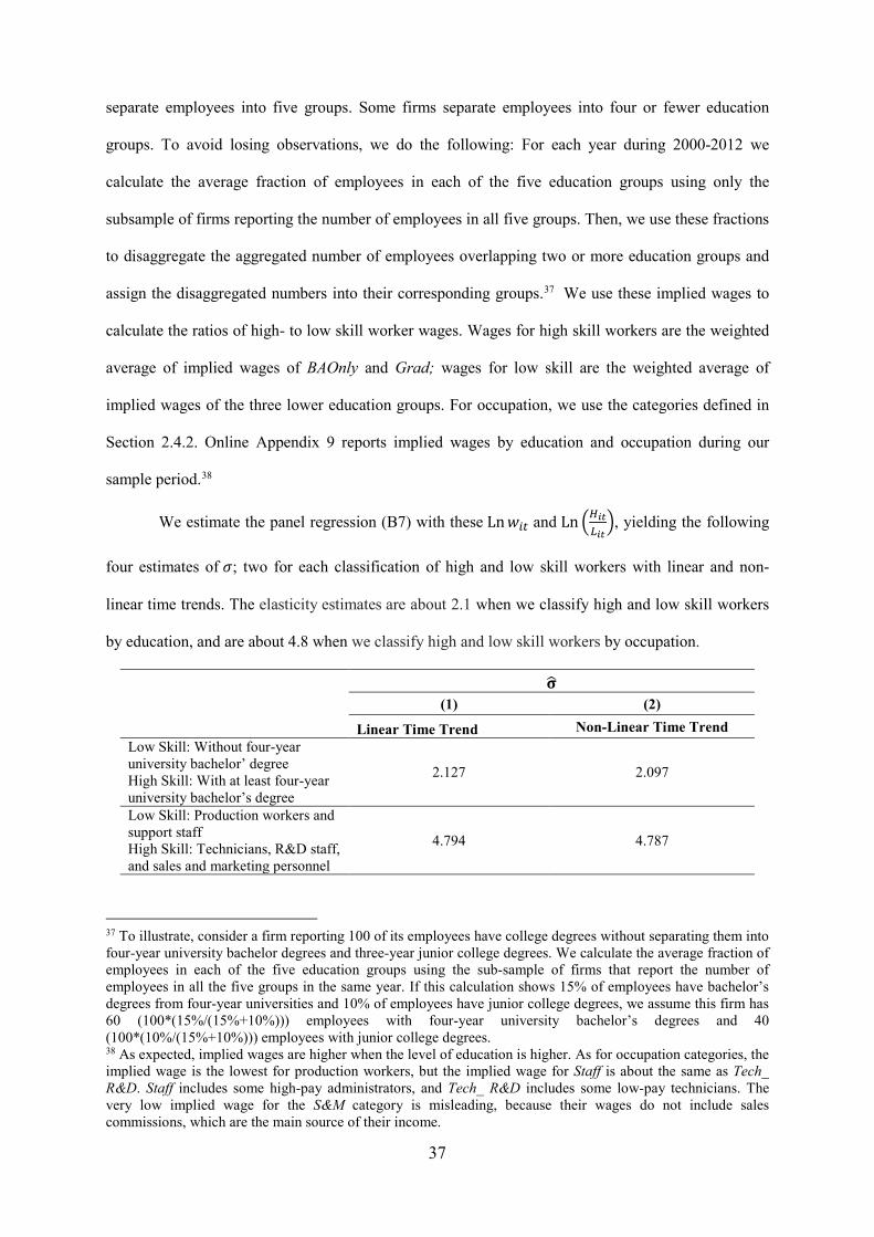
37
separate employees into five groups. Some firms separate employees into four or fewer education
groups. To avoid losing observations, we do the following: For each year during 2000-2012 we
calculate the average fraction of employees in each of the five education groups using only the
subsample of firms reporting the number of employees in all five groups. Then, we use these fractions
to disaggregate the aggregated number of employees overlapping two or more education groups and
assign the disaggregated numbers into their corresponding groups.37 We use these implied wages to
calculate the ratios of high- to low skill worker wages. Wages for high skill workers are the weighted
average of implied wages of BAOnly and Grad; wages for low skill are the weighted average of
implied wages of the three lower education groups. For occupation, we use the categories defined in
Section 2.4.2. Online Appendix 9 reports implied wages by education and occupation during our
sample period.38
We estimate the panel regression (B7) with these Ln𝑤𝑤𝑖𝑖𝑇𝑇 and Ln �𝐻𝐻𝑖𝑖𝑖𝑖𝐿𝐿𝑖𝑖𝑖𝑖�, yielding the following
four estimates of 𝜎𝜎; two for each classification of high and low skill workers with linear and non-
linear time trends. The elasticity estimates are about 2.1 when we classify high and low skill workers
by education, and are about 4.8 when we classify high and low skill workers by occupation.
𝛔𝛔� (1) (2) Linear Time Trend Non-Linear Time Trend Low Skill: Without four-year university bachelor’ degree 2.127 2.097 High Skill: With at least four-year university bachelor’s degree Low Skill: Production workers and support staff 4.794 4.787 High Skill: Technicians, R&D staff, and sales and marketing personnel
37 To illustrate, consider a firm reporting 100 of its employees have college degrees without separating them into four-year university bachelor degrees and three-year junior college degrees. We calculate the average fraction of employees in each of the five education groups using the sub-sample of firms that report the number of employees in all the five groups in the same year. If this calculation shows 15% of employees have bachelor’s degrees from four-year universities and 10% of employees have junior college degrees, we assume this firm has 60 (100*(15%/(15%+10%))) employees with four-year university bachelor’s degrees and 40 (100*(10%/(15%+10%))) employees with junior college degrees. 38 As expected, implied wages are higher when the level of education is higher. As for occupation categories, the implied wage is the lowest for production workers, but the implied wage for Staff is about the same as Tech_ R&D. Staff includes some high-pay administrators, and Tech_ R&D includes some low-pay technicians. The very low implied wage for the S&M category is misleading, because their wages do not include sales commissions, which are the main source of their income.

38
References
Acemoglu, Daron, 2002, Technological Change, Inequality, and the Labor Market, Journal of Economic Literature 40, 7-72.
Acemoglu, Daron, and Amy Finkelstein, 2008, Input and Technology Choices in Regulated Industries: Evidence from the Health Care Sector, Journal of Political Economy 116, 837-880.
Acemoglu, Daron, and David Autor, 2011, Skills, Tasks and Technologies: Implications for Employment and Earnings. In: David Card and Orley Ashenfelter (Eds.), Handbook of Labor Economics, Vol. 4b, Elsevier/North-Holland, Amsterdam, Chapter 12, 1043-1171.
Acemoglu, Daron, and Pascual Restrepo, 2017, Robots and Jobs: Evidence from US Labor Markets. Available at https://papers.ssrn.com/sol3/papers.cfm?abstract_id=2940245.
Acemoglu, Daron, and Pascual Restrepo, 2018, Artificial Intelligence, Automation and Work, NBER Working Paper No. 24196.
Acharya, Viral V., Tim Eisert, Christian Eufinger, and Christian Hirsch, 2018, Real Effects of the Sovereign Debt Crisis in Europe: Evidence from Syndicated Loans, Review of Financial Studies 31(8), 2856-2896.
Akerman, Anders, Ingvil Gaarder, and Magne Mogstad, 2015, The Skill Complementarity of Broadband Internet, Quarterly Journal of Economics 130, 1781-1824.
Almeida, Heitor, Vyacheslav Fos, and Mathias Kronlund, 2016, The Real Effects of Share Repurchases, Journal of Financial Economics 119, 168-185.
Agrawal, Ashwini, and Prasanna Tambe, forthcoming, Private Equity and Workers’ Career Paths: The Role of Technological Change, Review of Financial Studies.
Atanassov, Julian, and E. Han Kim, 2009, Labor and Corporate Governance: International Evidence from Restructuring Decisions, Journal of Finance 64, 341-374.
Autor, David H., and David Dorn, 2013, The Growth of Low-Skill Service Jobs and the Polarization of the US Labor Market, American Economic Review 103, 1553-1597.
Autor, David H., and Michael J. Handel, 2013, Putting Tasks to the Test: Human Capital, Job Tasks, and Wages, Journal of Labor Economics 31, 59-96.
Autor, David H., Lawrence F. Katz, and Melissa S. Kearney, 2006, The Polarization of the U.S. Labor Market, American Economics Review 96, 189-194.
Autor, David H., Lawrence F. Katz, and Alan B. Krueger, 1998, Computing Inequality: Have Computers Changed the Labor Market? Quarterly Journal of Economics 113, 1169-1213.
Autor, David. H., and Anna Salomons, 2017, Robocalypse Now—Does Productivity Growth Threaten Employment? Available at: https://ideas.repec.org/h/nbr/nberch/14019.html.
Bai, Chong-En, Jiangyong Lu, and Zhigang Tao, 2006, The Multitask Theory of State Enterprise Reform: Empirical Evidence from China, American Economic Review 96, 353-357.
Bai, John (Jianqiu), Daniel Carvalho, and Gordon M. Phillps, 2018, The Impact of Bank Credit on Labor Reallocation and Aggregate Industry Productivity, Journal of Finance 73, 2787-2836.
Beck, Thorsten, Ross Levine, and Alexey Levkov, 2010, Big Bad Banks? The Winners and Losers from Bank Deregulation in the United States, Journal of Finance 65, 1637-1667.
Benmelech, Efraim, Nittai K. Bergman, and Amit Seru, 2011, Financing Labor, NBER working Paper. Bentolila, Samuel, Marcel Jansen, and Gabriel Jimenez, 2018, When Credit Dries Up: Job Losses in
the Great Recession, Journal of the European Economic Association 16, 650-695. Berk, Jonathan B., Richard Stanton, and Josef Zechner, 2010, Human Capital, Bankruptcy, and
Capital Structure, Journal of Finance 65, 891-926. Bernstein, Shai, 2015, Does Going Public Affect Innovation? Journal of Finance 70, 1365-1403. Bertrand, Marianne, and Sendhi Mullainathan, 2003, Enjoying the Quiet Life? Corporate Governance
and Managerial Preferences, Journal of Political Economy 111, 1043-1075. Borisov, Alexander, Andrew Ellul, and Merih Sevilir, 2017, Access to Public Capital Markets and
Employment Growth, SSRN-id2178101. Bronars, Stephen G. and Donald R. Deere, 1991, The Threat of Unionization, the Use of Debt, and the
Preservation of Shareholder Wealth, Quarterly Journal of Economics 106, 231-254. Brown, James R., Steven M. Fazzari, and Bruce C. Petersen, 2009, Financing Innovation and Growth:
Cash Flow, External Equity, and the 1990s R&D Boom, Journal of Finance 64, 151-186. Bryson, Alex, John Forth, and Minghai Zhou, 2014, Same or Different? The CEO Labour Market in

39
China’s Public Listed Companies, Economic Journal 124, F90-F108. Campello, Murillo, John R. Graham, and Campbell R. Harvey. 2010, The Real Effects of Financial
Constraints: Evidence from a Financial Crisis. Journal of Financial Economics 97, 470–87. Card, David, 1999, The Causal Effect of Education on Earnings, In: David Card and Orley
Ashenfelter (Eds.), Handbook of Labor Economics, Vol. 3a, Elsevier/North-Holland, Amsterdam, Chapter 30, 1801-1863.
Card, David, 2001, Immigrant Inflows, Native Outflows, and the Local Labor Market Impacts of Higher Immigration, Journal of Labor Economics 19, 22-64.
Card, David, and John E. DiNardo, 2002, Skill-biased Technological Change and Rising Wage Inequality: Some Problems and Puzzles, Journal of Labor Economics 20, 733-783.
Card, David, and Thomas Lemieux, 2002, Can Falling Supply Explain the Rising Return to College for Younger Men? A Cohort-Based Analysis, Quarterly Journal of Economics 116, 705-746.
Carvalho, Daniel, 2014, The Real Effects of Government-Owned Banks: Evidence from an Emerging Market, Journal of Finance, 577-609.
Chemmanur, Thomas, Yingmei Cheng, and Tianming Zhang, 2013, Human Capital, Capital Structure, and Employee Pay: An Empirical Analysis, Journal of Financial Economics 110, 478-502.
Chodorow-Reich, Gabriel, 2014, The Employment Effects of Credit Market Disruptions: Firm-Level Evidence from the 2008-2009 Financial Crisis, Quarterly Journal of Economics 129, 1-59.
Cingano, Federico, Francesco Manaresi, and Enrico Sette, 2016, Does Credit Crunch Investment Down? New Evidence on the Real Effect of the Bank-Lending Channel, Review of Financial Studies 29, 2737-2773.
Cronqvist, Henrik, Fredrik Heyman, Mattias Nilsson, Helena Svaleryd, and Jonas Vlachos, 2009, Do Entrenched Managers Pay Their Workers More? Journal of Finance 64, 309-339.
DeAngelo, Harry, Linda DeAngelo, and René Stulz, 2010, Seasoned Equity Offerings, Market Timing, and the Corporate Lifecycle, Journal of Financial Economics 95, 275-295.
Eckbo, B. Espen, Ronald W. Masulis, and Øyvind Norli, 2000, Seasoned Public Offerings: Resolution of the ‘New Issues Puzzle’, Journal of Financial Economics 56, 251-291.
Giroud, Xavier, and Holger M. Mueller, 2017, Firm Leverage, Consumer Demand, and Employment Losses During the Great Recession, Quarterly Journal of Economics 271-316.
Gustafson, Matthew T., and Peter Iliev, 2017, The Effects of Removing Barriers to Equity Issuance, Journal of Financial Economics 124, 580-598.
Hall, Brownyn H., and Josh Lerner, 2010, The Financing of R&D and Innovation, In: Brownyn H. Hall and Nathan Rosenberg (Eds.), Handbooks in Economics of Innovation, Vol. 1, Elsevier/North-Holland, Amsterdam, Chapter 14, 609-639.
Hau, Harald, and Sandy Lai, 2013, Real Effects of Stock Underpricing, Journal of Financial Economics 108, 392-408.
Hawkins, William B., Ryan Michaels, and Jiyoon Oh, 2015, The Joint Dynamics of Capital and Employment as the Plant Level, Working Paper.
Heckman, James J., Lance Lochner, and Christopher Taber, 1998, "Explaining Rising Wage Inequality: Explorations with a Dynamic General Equilibrium Model of Labor Earnings with Heterogeneous Agents." Review of Economic Dynamics 1, 1-58.
Hershbein, Brad, and Lisa Kahn, 2018, Do Recessions Accelerate Routine-Biased Technology Change? Evidence from Vacancy Postings, American Economic Review 108, 1737-1772.
Hsu, Po-Hsuan, Xuan Tian, and Yan Zu, 2014, Financial Development and Innovation: Cross-country Evidence, Journal of Financial Economics 112, 116-135.
Jensen, Michael C., 1986, Agency Costs of Free Cash Flow, Corporate Finance, and Takeovers, American Economic Review 76, 323-329.
Jung, Kooyul, Yong-Cheol Kim, and René M. Stulz, 1996, Timing, Investment Opportunities, Managerial Discretion, and the Security Issue Decision, Journal of Financial Economics 42, 159-185.
Kahn, James A., and Jong-Soo Lim, 1998, Skilled Labor-Augmenting Technological Progress in U.S. Manufacturing, Quarterly Journal of Economics 113, 1281-1308.
Katz, Lawrence F., and Kevin M. Murphy, 1992, “Changes in Relative Wages, 1963–1987: Supply and Demand Factors.” Quarterly Journal of Economics 107, 35–78.

40
Kim, E. Han, and Paige Ouimet, 2014, Broad-Based Employee Stock Ownership: Motives and Outcomes, Journal of Finance 69, 1273-1319.
Kim, E. Han, and Amiyatosh Purnanandam, 2014, Seasoned Equity Offerings, Corporate Governance, and Investments, Review of Finance 18, 1023-1057.
Kim, Woojin, and Michael S. Weisbach, 2008, Motivations for Public Equity Offers: An International Perspective, Journal of Financial Economics 87, 281-307.
Letterie, Wilko, Gerard Pfann, and J. Michael Polder, 2004, Factor Adjustment Spikes and Interrelation: An Empirical Investigation, Economics Letters, 85(2): 145-150.
Levinsohn, James, and Amil Petrin, 2003, Estimating Production Functions Using Inputs to Control for Unobservables, Review of Economic Studies 70, 317-341
Lewis, Ethan, 2011, Immigration, Skill Mix, and Capital-Skill Complementarity, Quarterly Journal of Economics 126, 1029-1069.
Matsa, David A., 2018, Capital Structure and a Firm’s Workforce, Annual Review of Financial Economics 10, 387-412.
McCrary, Justin, 2008, Manipulation of the Running Variable in the Regression Discontinuity Design: A Density Test, Journal of Econometrics 142, 698-714.
McLean, R. David, 2011, Share Issuance and Cash Savings, Journal of Financial Economics 99, 693-715.
Michaels, Ryan, T. Beau Page, and Toni Whited, Forthcoming, Labor and Capital Dynamics under Financing Frictions, Review of Finance.
Midrigan, Virgiliu, and Daniel Yi Xu, 2014, Finance and Misallocation: Evidence from Plant-Level Data, American Economic Review 104 (2), 422-458.
Pagano, Marco, Fabio Panetta, and Luigi Zingales, 1998, Why Do Companies Go Public? An Empirical Analysis, Journal of Finance 53, 27-64.
Perotti, Enrico C., and Kathlyn E. Spier, 1993, Capital Structure as a Bargaining Tool: The Role of Leverage in Contract Renegotiation, American Economic Review 83, 1131-1141.
Rauh, Joshua, 2006, Investment and Financing Constraints: Evidence from the Funding of Corporate Pension Plans, Journal of Finance 61, 33-72.
Tuzel, Selale, and Miao Ben Zhang, 2018, Economic Stimulus at the Expense of Routine-Task Jobs, Working Paper.
Wang, Qian, T. J. Wong, and Lijun Xia, 2008, State Ownership, the Institutional Environment, and Auditor Choice: Evidence from China, Journal of Accounting and Economics 46, 112-134.
Wen, Jiabao, 2010 年政府工作报告 http://www.gov.cn/2010lh/content_1555767.htm. Wooldridge, Jeffrey, 2010, Econometric Analysis of Cross Section and Panel Data, Cambridge, MIT
Press. Zhang, Junsen, Yaohui Zhao, Albert Park, and Xiaoqing Song, 2005, Economic Returns to Schooling
in Urban China, 1988 to 2001, Journal of Comparative Economics 33, 730-752.

41
Table 1: Sample and SEOs by Year. The sample includes Chinese firms listed on Shanghai and Shenzhen Stock Exchanges over 2000 - 2012. Financial firms, firms with fewer than 100 employees, ST (special treatment), and *ST firms are excluded. Firms are classified as ST or *ST if they have two (ST) or three (*ST) consecutive years of negative net profits. Column (1) shows the number of firms in the full sample by year. Column (2) shows the number of public offerings by year of receiving SEO proceeds.
Year Full Number of SEOs (1) (2)
2000 885 154 2001 951 131 2002 1,002 44 2003 1,059 38 2004 1,153 32 2005 1,172 7 2006 1,204 7 2007 1,323 28 2008 1,395 43 2009 1,485 18 2010 1,830 20 2011 2,120 23 2012 2,259 12 Total 17,838 557

42
Table 2: Summary Statistics. This table reports summary statistics for variables used in the panel regressions. Online Appendix 3 provides variable definitions and data sources. VARIABLES Mean Std. Dev. Min Max SEO 0.088 0.283 0.000 1.000 SEO_Proceed (1,000,000) 725.902 1595.407 34.656 23947.61 SEOIneligible 0.155 0.362 0.000 1.000 EMP (100) 45.916 176.742 1.000 5528.100 Production 2228.760 9157.168 0.000 337036.000 Staff 320.840 1822.266 10.000 85228.000 Tech_R&D 650.142 3731.857 0.000 199531.000 S&M 503.142 2862.225 0.000 94476.000 Finance 95.998 472.648 0.000 14445.000 Others 861.889 5531.349 0.000 226361.000 Grad 124.597 767.276 0.000 24642.000 BA 868.775 4826.496 0.000 152840.000 NBA 4205.349 16702.3 8.000 427676.000 %_Production 0.483 0.284 0.000 0.997 %_Staff 0.093 0.109 0.001 0.998 %_Tech_R&D 0.175 0.158 0.000 0.987 %_S&M 0.130 0.162 0.000 0.996 %_Finance 0.034 0.035 0.000 0.788 %_Others 0.173 0.259 0.000 1.000 %_Grad 0.031 0.043 0.000 0.237 %_BA 0.202 0.178 0.000 0.959 Fixed_Tech (1,000,000) 148.853 1475.197 0.000 91309.090 Intangible_Tech (10,000) 978.125 6733.577 0.000 197295.200 Capx (1,000,000) 479.913 4753.238 0.001 247650.400 AWAGE (10,000) 6.928 11.691 0.013 658.944 AWAGE_NonExe (10,000) 7.054 12.352 0.011 723.361 AEXEPAY (10,000) 20.192 20.009 0.360 506.227 Payroll (1,000,000) 296.153 1908.561 0.039 108031.000 Payroll_NonExe (1,000,000) 306.816 1964.043 0.019 108015.900 Payroll_Exe (1,000,000) 2.876 3.534 0.022 111.370 ROA 0.035 0.111 -4.051 6.109 Sales_GR 0.228 0.497 -0.609 3.379 Sales/Employees (1,000,000) 1.105 2.878 0.000 130.867 TFP 0.003 0.336 -1.217 0.976 P3_PR 0.766 0.827 0.000 4.085 P3_PR_D 0.027 0.161 0.000 1.000 NYEAR_LISTED 7.011 5.013 0.000 22.000 Ln(MIN_WAGE) 640.329 207.828 208.540 1085.329 LAWSCORE 7.784 3.916 0.000 16.610 Labor_Law_Effect 3.689 3.850 0.000 13.312 SALES (1,000,000) 4517.473 39862.920 0.003 2085363.000 %_LARGEST_SH 0.390 0.163 0.022 0.894 DIV_PR 0.259 0.306 0.000 1.500 %_STATE_OWN 0.215 0.252 0.000 0.886 %_IND_DIR 0.306 0.127 0.000 0.833 %_NONTRD_SH 0.212 0.296 0.000 0.913 LEVERAGE 0.456 0.201 0.047 0.889 PPE/TA 0.320 0.201 0.000 0.975

43
Table 3: Total Firm-level Employment and Employees by Occupation or Education. This table reports the second-stage estimation of the impacts that SEOs have on firm-level employment. The dependent variable is the number of all employees in Column (1), production workers in Column (2), support staff in Column (3), technicians and R&D employees in Column (4), sales and marketing forces in Column (5), finance staff in Column (6), employees in uncategorized occupations in Column (7), employees with post-graduate degrees in Column (8), employees with four-year university bachelor’s degrees and above in Column (9), and employees without four-year university bachelor’s degrees in Column (10). All dependent variables, except Column (1), are the log of one plus the number of employees. All regressions include firm- and year fixed effects. Online Appendix 3 provides variable definitions and data sources. The sample period covers 2000 – 2012. Bootstrapped standard errors are reported in parentheses. Coefficients marked with *, **, and *** are significant at 10%, 5%, and 1%, respectively.
Ln (EMP)
Ln (Production)
Ln (Staff)
Ln (Tech_R&D)
Ln (S&M)
Ln (Finance)
Ln (Others)
Ln (Grad)
Ln (BA)
Ln (NBA)
VARIABLES (1) (2) (3) (4) (5) (6) (7) (8) (9) (10) 𝑆𝑆𝑆𝑆𝑆𝑆� -0.091** -0.252** -0.463*** 0.133** 0.103* 0.008 -0.070 0.111* 0.004 -0.174***
(0.043) (0.102) (0.097) (0.056) (0.062) (0.052) (0.218) (0.065) (0.061) (0.053)
P3_PR 0.011* 0.045*** 0.038** 0.002 0.016 -0.004 -0.030 -0.021* 0.018 0.014*
(0.006) (0.014) (0.015) (0.010) (0.015) (0.008) (0.031) (0.011) (0.012) (0.007)
P3_PR_D -0.017 -0.025 0.063 -0.063* 0.035 -0.035 0.052 -0.075 -0.079** 0.002
(0.024) (0.056) (0.073) (0.033) (0.033) (0.024) (0.129) (0.053) (0.034) (0.030)
Ln(NYEAR_LISTED) 0.117*** 0.129** 0.138** 0.076** 0.076** 0.069*** 0.445*** 0.040 0.054* 0.130***
(0.022) (0.058) (0.057) (0.032) (0.034) (0.023) (0.107) (0.048) (0.030) (0.027)
Ln(MIN_WAGE) -0.265*** -0.175 -0.213* -0.227*** -0.106 -0.160*** 0.036 0.255** -0.002 -0.432***
(0.058) (0.117) (0.116) (0.075) (0.086) (0.058) (0.239) (0.121) (0.091) (0.084)
LAWSCORE -0.012** 0.011 0.005 0.003 0.014* -0.011** -0.069*** -0.022* -0.009 -0.023***
(0.005) (0.011) (0.012) (0.007) (0.008) (0.005) (0.022) (0.013) (0.008) (0.009)
Labor_Law_Effect -0.004 -0.041*** 0.011 0.006 -0.025** 0.002 0.050*** -0.037*** -0.020*** 0.012**
(0.003) (0.008) (0.011) (0.006) (0.012) (0.005) (0.017) (0.005) (0.005) (0.005)
Ln(SALES) 0.421*** 0.326*** 0.259*** 0.396*** 0.415*** 0.319*** 0.325*** 0.393*** 0.421*** 0.446***
(0.012) (0.027) (0.016) (0.016) (0.016) (0.012) (0.036) (0.020) (0.015) (0.016)
%_LARGEST_SH -0.094 -0.273* 0.242** 0.023 0.082 0.131* 0.084 -0.092 0.074 -0.346**
(0.075) (0.163) (0.123) (0.109) (0.136) (0.074) (0.316) (0.138) (0.110) (0.142)
DIV_PR 0.005 0.008 0.008 0.002 -0.002 0.003 -0.004 -0.002 0.005 0.006
(0.010) (0.013) (0.021) (0.012) (0.013) (0.010) (0.019) (0.016) (0.013) (0.009)
%_STATE_OWN 0.125*** 0.007 0.074 0.076 -0.007 0.060* 0.221* 0.023 0.148*** 0.143***
(0.028) (0.076) (0.084) (0.054) (0.091) (0.035) (0.123) (0.055) (0.050) (0.045)
%_IND_DIR 0.039 -0.190* -0.042 0.227*** 0.192** 0.079 0.150 0.034 0.023 0.063
(0.043) (0.112) (0.116) (0.081) (0.085) (0.049) (0.186) (0.097) (0.084) (0.075)
%_NONTRD_SH 0.040 0.046 -0.102 -0.077 -0.056 -0.012 0.027 -0.016 -0.034 0.037
(0.044) (0.092) (0.105) (0.062) (0.048) (0.041) (0.167) (0.090) (0.058) (0.062)
Leverage 0.261*** -0.130 0.276*** 0.208*** 0.202** 0.429*** 0.581*** 0.228** 0.267*** 0.239***
(0.041) (0.115) (0.105) (0.059) (0.098) (0.051) (0.223) (0.110) (0.066) (0.064)
PPE/TA 0.530*** 0.963*** 0.451*** 0.272*** -0.236** -0.078 -0.501** -0.056 0.178** 0.702***
(0.050) (0.114) (0.094) (0.073) (0.114) (0.049) (0.213) (0.118) (0.085) (0.089)
Constant 1.455*** 4.976*** 3.113*** 4.067*** 2.770*** 2.387*** 1.118 -1.390* 2.148*** 6.701***
(0.348) (0.728) (0.703) (0.474) (0.527) (0.359) (1.532) (0.771) (0.555) (0.520)
Firm & Year FE Y Y Y Y Y Y Y Y Y Y Observations 16,964 16,964 16,964 13,916 10,576 13,326 16,964 8,109 11,650 11,650

44
Table 4: Employee Composition by Occupation or Education. This table reports the second-stage estimation of the impacts that SEOs have on the employee composition by occupation or education. The dependent variable is the percentage of production workers in Column (1), support staff in Column (2), technicians and R&D employees in Column (3), sales and marketing forces in Column (4), finance staff in Column (5), employees in uncategorized occupations in Column (6), employees with post-graduate degrees in Column (7), and employees with four-year university Bachelor’s degrees and above in Column (8). All regressions include firm- and year fixed effects. Online Appendix 3 provides variable definitions and data sources. The sample period covers 2000 – 2012. Bootstrapped standard errors are reported in parentheses. Coefficients marked with *, **, and *** are significant at 10%, 5%, and 1%, respectively. %_Production %_Staff %_Tech_R&D %_S&M %_Finance %_Others %_Grad %_BA VARIABLES (1) (2) (3) (4) (5) (6) (7) (8) SEO� -0.037*** -0.011* 0.038*** 0.023*** 0.004* 0.007 0.006** 0.018**
(0.014) (0.007) (0.010) (0.005) (0.002) (0.018) (0.003) (0.007)
P3_PR 0.005** 0.002* -0.001 0.000 -0.001*** -0.008*** -0.000 0.001
(0.003) (0.001) (0.001) (0.001) (0.000) (0.003) (0.000) (0.001)
P3_PR_D 0.001 0.002 -0.010** 0.001 -0.002** 0.002 0.000 -0.010**
(0.009) (0.004) (0.004) (0.003) (0.001) (0.010) (0.001) (0.004)
Ln(NYEAR_LISTED) -0.002 -0.004 -0.011** -0.009** -0.001 0.023** -0.002 -0.002
(0.007) (0.004) (0.005) (0.004) (0.001) (0.009) (0.002) (0.005)
Ln(MIN_WAGE) 0.004 0.006 -0.003 -0.002 0.001 0.008 0.005 0.038***
(0.019) (0.008) (0.013) (0.012) (0.002) (0.025) (0.003) (0.011)
LAWSCORE 0.003* -0.000 0.002** 0.000 -0.000 -0.007*** -0.000 0.001
(0.002) (0.001) (0.001) (0.001) (0.000) (0.002) (0.000) (0.001)
Labor_Law_Effect -0.006*** 0.002*** 0.001 -0.003*** 0.001 0.004** -0.001*** -0.005***
(0.001) (0.001) (0.001) (0.001) (0.000) (0.002) (0.000) (0.001)
Ln(SALES) 0.003 -0.006*** -0.004** 0.002 -0.002*** 0.004 -0.001 -0.003
(0.003) (0.002) (0.002) (0.002) (0.001) (0.004) (0.001) (0.002)
%_LARGEST_SH -0.055** 0.036*** 0.027 0.024* 0.018*** 0.012 0.007* 0.067***
(0.025) (0.011) (0.018) (0.014) (0.003) (0.027) (0.004) (0.017)
DIV_PR 0.001 0.000 -0.001 -0.000 -0.000 0.000 -0.000 -0.000
(0.003) (0.001) (0.002) (0.001) (0.000) (0.004) (0.001) (0.001)
%_STATE_OWN -0.003 -0.013*** -0.008 -0.023*** -0.002 0.019* -0.003 0.002
(0.011) (0.005) (0.005) (0.005) (0.001) (0.011) (0.002) (0.007)
%_IND_DIR -0.054*** 0.013* 0.029*** 0.034*** -0.002 0.010 -0.003 -0.014
(0.019) (0.008) (0.010) (0.012) (0.003) (0.024) (0.003) (0.012)
%_NONTRD_SH -0.001 0.004 -0.006 -0.006 0.000 0.008 0.005 -0.011
(0.018) (0.008) (0.008) (0.011) (0.002) (0.017) (0.003) (0.010)
Leverage -0.081*** 0.016* -0.001 0.003 0.009*** 0.049*** 0.004 0.009
(0.015) (0.010) (0.012) (0.007) (0.002) (0.019) (0.003) (0.010)
PPE/TA 0.168*** -0.012 -0.030** -0.054*** -0.024*** -0.113*** -0.015*** -0.084***
(0.018) (0.009) (0.012) (0.017) (0.002) (0.023) (0.003) (0.013)
Constant 0.464*** 0.047 0.214** 0.146** 0.033*** 0.129 0.006 -0.048
(0.112) (0.047) (0.086) (0.067) (0.013) (0.148) (0.022) (0.070)
Firm & Year FE Y Y Y Y Y Y Y Y Observations 16,964 16,964 13,916 10,576 13,326 16,964 8,109 11,650

45
Table 5: Technology Adoption. This table reports the second-stage estimation of the effects of SEOs on expenditures on technology-related fixed- and intangible assets and on general capital expenditures. The dependent variable is the log of one plus expenditures on machines and equipment in Column (1), the log of one plus expenditures on technology-related intangible assets in Columns (2), and the log of capital expenditures in Column (3). Online Appendix 3 provides variable definitions and data sources. The sample period covers 2003-2012 for Column (1), 2007-2012 for Column (2), and 2000-2012 for Column (3). All regressions include firm- and year fixed effects. Bootstrapped standard errors are reported in parentheses. Coefficients marked with *, **, and *** are significant at 10%, 5%, and 1%, respectively.
Ln(Fixed_Tech) Ln(Intangible_Tech) Ln(Capx)
VARIABLES (1) (2) (3) SEO� 0.272*** 0.363* 0.265***
(0.094) (0.188) (0.091)
P3_PR 0.005 -0.031 0.050***
(0.019) (0.050) (0.014)
P3_PR_D -0.149*** 0.315 -0.399***
(0.057) (0.252) (0.060)
Ln(NYEAR_LISTED) -0.192*** 0.206 -0.435***
(0.047) (0.161) (0.040)
Ln(MIN_WAGE) 0.029 -0.087 0.013
(0.183) (0.556) (0.118)
LAWSCORE -0.030
-0.006
(0.020)
(0.010)
Labor_Law_Effect -0.030*** 0.004 -0.041***
(0.011) (0.034) (0.009)
Ln(SALES) 0.552*** 0.443*** 0.801***
(0.025) (0.091) (0.024)
%_LARGEST_SH 0.237 0.340 0.476***
(0.167) (0.746) (0.169)
DIV_PR 0.001 0.003 0.008
(0.024) (0.044) (0.019)
%_STATE_OWN 0.128* 0.316 0.085
(0.066) (0.200) (0.053)
%_IND_DIR -0.044 -0.221 0.199
(0.186) (0.417) (0.132)
%_NONTRD_SH -0.148* -0.765 -0.655***
(0.085) (1.364) (0.104)
Leverage 0.693*** 0.103 0.044
(0.128) (0.412) (0.111)
PPE/TA 2.225*** 0.658 2.862***
(0.154) (0.408) (0.117)
Constant -2.332** 0.825 -1.788***
(1.166) (3.413) (0.692)
Firm & Year FE Y Y Y Observations 14,453 6,187 17,099

46
Table 6: Firm Performance. This table reports the second-stage estimation of the impacts that SEOs have on firm performance. The dependent variable is ROA in Column (1), sales growth rate in Column (2), sales per employee in Column (3), and total factor productivity in Column (4). Online Appendix 3 provides variable definitions and data sources. The sample period covers 2000-2012 . All regressions include firm- and year fixed effects. Bootstrapped standard errors are reported in parentheses. Coefficients marked with *, **, and *** are significant at 10%, 5%, and 1%, respectively.
ROA Sales_GR Sales/Employees TFP
VARIABLES (1) (2) (3) (4) SEO� 0.018*** 0.213*** 0.847** 0.094***
(0.007) (0.041) (0.425) (0.027)
P3_PR -0.002*** -0.024*** -0.023 -0.001
(0.000) (0.005) (0.024) (0.004)
P3_PR_D -0.014** 0.026 0.052 -0.027*
(0.006) (0.026) (0.063) (0.015)
Ln(NYEAR_LISTED) -0.012*** -0.124*** -0.340*** -0.095***
(0.003) (0.017) (0.102) (0.013)
Ln(MIN_WAGE) 0.008 -0.104* 0.111 0.044
(0.007) (0.056) (0.154) (0.033)
LAWSCORE -0.002*** -0.010** 0.158*** -0.006**
(0.001) (0.004) (0.029) (0.003)
Labor_Law_Effect 0.002*** 0.005 0.003 -0.002
(0.000) (0.004) (0.011) (0.002)
Ln(SALES) 0.018*** 0.231*** 0.698*** 0.374***
(0.003) (0.011) (0.051) (0.008)
%_LARGEST_SH 0.052*** 0.459*** 0.563*** -0.007
(0.010) (0.077) (0.207) (0.044)
DIV_PR -0.000 -0.004 -0.007 -0.004
(0.001) (0.008) (0.027) (0.007)
%_STATE_OWN -0.005 0.077** -0.315** -0.101***
(0.004) (0.033) (0.134) (0.018)
%_IND_DIR -0.007 -0.020 -0.131 -0.042
(0.008) (0.047) (0.205) (0.033)
%_NONTRD_SH -0.005 -0.142*** -0.064 0.021
(0.009) (0.040) (0.229) (0.031)
Leverage -0.159*** 0.153*** 0.107 -0.275***
(0.007) (0.053) (0.203) (0.034)
PPE/TA -0.049*** -0.087* -1.178*** -0.185***
(0.009) (0.051) (0.237) (0.040)
Constant -0.042 -0.579* -4.781*** -2.244***
(0.048) (0.339) (0.934) (0.203)
Firm & Year FE Y Y Y Y Observations 16,916 17,136 16,964 16,827

47
Table 7: Average Wages. This table reports the second-stage estimation of the impacts that SEOs have on average wages (total payroll/total number of employees). The dependent variable is the log of the average wage of all employees in Column (1), all non-executive employees in Column (2), all executives in Column (3). Online Appendix 3 provides variable definitions and data sources. The sample period covers 2000 – 2012 for Column (1) and 2001 – 2012 for Columns (2) – (3). All regressions include firm- and year fixed effects. Bootstrapped standard errors are reported in parentheses. Coefficients marked with *, **, and *** are significant at 10%, 5%, and 1%, respectively.
Ln(AWAGE) Ln(AWAGE_NonExe) Ln(AEXEPAY)
VARIABLES (1) (2) (3) SEO� 0.065* 0.089** 0.025
(0.037) (0.044) (0.032)
P3_PR 0.015*** 0.011** 0.014***
(0.006) (0.005) (0.005)
P3_PR_D 0.031 0.028 -0.078***
(0.025) (0.020) (0.022)
Ln(NYEAR_LISTED) -0.009 -0.016 -0.075***
(0.013) (0.021) (0.017)
Ln(MIN_WAGE) 0.296*** 0.295*** 0.176***
(0.047) (0.051) (0.050)
LAWSCORE -0.007* -0.006 -0.030***
(0.004) (0.006) (0.005)
Labor_Law_Effect 0.003 0.001 0.014***
(0.003) (0.004) (0.003)
Ln(SALES) 0.120*** 0.124*** 0.196***
(0.011) (0.010) (0.008)
%_LARGEST_SH 0.220*** 0.257*** 0.011
(0.055) (0.064) (0.051)
DIV_PR 0.001 0.001 0.005
(0.012) (0.011) (0.006)
%_STATE_OWN 0.079*** 0.069*** -0.019
(0.024) (0.020) (0.027)
%_IND_DIR -0.017 -0.022 -0.028
(0.045) (0.046) (0.042)
%_NONTRD_SH -0.058 -0.034 -0.030
(0.044) (0.047) (0.034)
Leverage -0.111*** -0.119*** -0.176***
(0.037) (0.043) (0.035)
PPE/TA -0.128*** -0.085 -0.193***
(0.042) (0.060) (0.040)
Constant -1.836*** -1.781*** -0.116
(0.288) (0.317) (0.310)
Firm & Year FE Y Y Y Observations 16,960 16,026 16,026

48
Table 8: Total Wages. This table reports the second-stage estimation of the impacts that SEOs have on total wages. The dependent variable is the log of total wages to all employees in Column (1), all non-executive employees in Column (2), all executives in Column (3). Online Appendix 3 provides variable definitions and data sources. The sample period covers 2000 – 2012 for Column (1) and 2001 – 2012 for Columns (2) – (3). All regressions include firm- and year fixed effects. Bootstrapped standard errors are reported in parentheses. Coefficients marked with *, **, and *** are significant at 10%, 5%, and 1%, respectively.
Ln(Payroll) Ln(Payroll_NonExe) Ln(Payroll_Exe)
VARIABLES (1) (2) (3) SEO� -0.035 -0.033 0.011
(0.035) (0.034) (0.033)
P3_PR 0.027*** 0.022*** 0.020***
(0.004) (0.005) (0.006)
P3_PR_D 0.017 0.021 -0.134***
(0.019) (0.018) (0.025)
Ln(NYEAR_LISTED) 0.107*** 0.109*** -0.060***
(0.015) (0.015) (0.021)
Ln(MIN_WAGE) 0.021 0.001 0.116**
(0.047) (0.042) (0.051)
LAWSCORE -0.020*** -0.021*** -0.022***
(0.003) (0.004) (0.004)
Labor_Law_Effect -0.001 0.000 0.015***
(0.003) (0.003) (0.004)
Ln(SALES) 0.538*** 0.545*** 0.226***
(0.011) (0.011) (0.011)
%_LARGEST_SH 0.165** 0.191*** 0.011
(0.064) (0.064) (0.077)
DIV_PR 0.006 0.006* 0.006
(0.004) (0.003) (0.007)
%_STATE_OWN 0.192*** 0.197*** -0.014
(0.022) (0.023) (0.025)
%_IND_DIR 0.012 -0.002 0.072
(0.034) (0.036) (0.048)
%_NONTRD_SH -0.024 -0.011 -0.117***
(0.042) (0.034) (0.043) Leverage 0.164*** 0.190*** -0.085*
(0.035) (0.041) (0.047)
PPE/TA 0.413*** 0.444*** -0.152***
(0.043) (0.054) (0.036)
Constant -0.323 -0.236 -2.285***
(0.287) (0.271) (0.313)
Firm & Year FE Y Y Y Observations 17,131 16,152 16,152

49
Table 9: Results of Pre-trend Placebo Tests. This table reports the results of placebo tests for pre-trends. Dependent variables in Columns (2) – (11) are the log of one plus the number of the relevant variables. Online Appendix 3 provides variable definitions and data sources. Robust standard errors clustered at the firm level are reported in parentheses. Coefficients marked with *, **, and *** are significant at 10%, 5%, and 1%, respectively.
Ln Ln Ln Ln Ln Ln Ln Ln Ln Ln Ln (Fixed_
SALES Sales
Ln Ln
(EMP) (Production) (Staff) (Tech_R&D) (S&M) (Finance) (Others) (Grad) (BA) (NBA) Tech) ROA _GR /Emp TFP (AWAGE) (Payroll)
VARIABLES (1) (2) (3) (4) (5) (6) (7) (8) (9) (10) (11) (12) (13) (14) (15) (16) (17) Affected*Year01 0.015 0.071 -0.132 -0.002 -0.000 0.056 -0.380 0.110 0.032 0.029
-0.008 0.028 -0.060 -0.018 -0.058 -0.027
(0.034) (0.100) (0.107) (0.055) (0.063) (0.041) (0.239) (0.160) (0.091) (0.070)
(0.006) (0.052) (0.093) (0.026) (0.038) (0.031)
Affected*Year02 -0.017 0.001 -0.130 -0.012 -0.102 0.021 -0.305 0.098 0.023 0.005
-0.010 0.021 -0.107 -0.006 -0.034 -0.038
(0.040) (0.112) (0.124) (0.064) (0.073) (0.049) (0.266) (0.176) (0.102) (0.087)
(0.006) (0.058) (0.130) (0.029) (0.040) (0.035)
Affected*Year03 -0.011 -0.024 -0.132 -0.102 -0.114 0.052 -0.449 0.001 -0.064 0.018
-0.010 0.053 -0.263 0.032 -0.062 -0.060
(0.044) (0.119) (0.130) (0.072) (0.081) (0.054) (0.275) (0.185) (0.106) (0.095)
(0.007) (0.061) (0.220) (0.031) (0.042) (0.037)
Affected*Year04 -0.025 -0.081 -0.105 -0.043 -0.132 0.025 -0.379 -0.079 -0.175 0.026 -0.007 -0.010 0.102 -0.220 0.053 -0.069 -0.080*
(0.050) (0.129) (0.138) (0.076) (0.084) (0.060) (0.297) (0.192) (0.115) (0.107) (0.143) (0.008) (0.065) (0.141) (0.033) (0.048) (0.044)
Affected*Year05 -0.009 -0.015 -0.161 -0.075 -0.132 0.049 -0.261 -0.044 -0.189 0.011 -0.150 -0.012 0.104 -0.229 0.046 -0.059 -0.055
(0.053) (0.139) (0.155) (0.081) (0.096) (0.063) (0.316) (0.204) (0.117) (0.114) (0.158) (0.008) (0.065) (0.155) (0.034) (0.051) (0.047)
Firm FE/YearFE Y Y Y Y Y Y Y Y Y Y Y Y Y Y Y Y Y Controls Y Y Y Y Y Y Y Y Y Y Y Y Y Y Y Y Y Observations 5,683 5,683 5,683 4,787 4,642 4,799 5,683 2,043 2,936 2,936 3,084 5,636 5,767 5,683 5,609 5,680 5,763 Adjusted R2 0.922 0.807 0.603 0.813 0.876 0.872 0.574 0.891 0.907 0.956 0.739 0.470 0.185 0.817 0.696 0.855 0.944

50
Table 10: Alternative Ways to Construct the Instrument and Definition of SEOs. This table reports the second-stage estimation results using alternative instruments and definition of SEOs. Column (1) lists the dependent variables. Only coefficients on the predicted SEO, standard errors, and sample sizes are reported for each robustness test. Column (2) turns on the instrument only for the firms treated by the 2006 regulation in 2006 and the firms treated by the 2008 regulation in 2008. Column (3) uses a one-year lag between the beginning of an SEO process and the availability of SEO proceeds. Column (4) relies only on the 2006 regulation to construct the instrument. Column (5) excludes small SEOs whose proceeds are in the bottom decile. Online Appendix 3 provides variable definitions and data sources. Online Appendix 4 reports the first-stage estimation results. Bootstrapped standard errors are reported in parentheses. Coefficients marked with *, **, and *** are significant at 10%, 5%, and 1%, respectively.
DEPENDENT VARIABLES
IV based on treatments only in
2006 and 2008 Using one-year lag IV based only on
the 2006 regulation Excluding small
SEOs
(1) (2) (3) (4) (5) Ln(EMP) -0.081** -0.094** -0.092** -0.095**
(0.038) (0.047) (0.046) (0.048)
N 16,964 16,964 16,964 16,964 Ln(Production) -0.232** -0.279** -0.092** -0.254**
(0.098) (0.109) (0.046) (0.102)
N 16,964 16,964 16,964 16,964 Ln(Staff) -0.456*** -0.509*** -0.467*** -0.478***
(0.105) (0.108) (0.121) (0.109)
N 16,964 16,964 16,964 16,964 Ln(Tech_R&D) 0.111* 0.116* 0.077 0.127**
(0.060) (0.067) (0.057) (0.060)
N 13,916 13,916 13,916 13,916 Ln(S&M) 0.103* 0.077 0.074 0.104*
(0.059) (0.081) (0.069) (0.061)
N 10,576 10,576 10,576 10,576 Ln(Finance) 0.003 0.007 0.006 0.006
(0.053) (0.057) (0.056) (0.048)
N 13,326 13,326 13,326 13,326 Ln(Others) -0.075 -0.016 -0.055 -0.056
(0.183) (0.225) (0.203) (0.211)
N 16,964 16,964 16,964 16,964 Ln(Grad) 0.108* 0.117* 0.117* 0.109*
(0.058) (0.064) (0.067) (0.057)
N 8,109 8,109 8,109 8,109 Ln(BA) -0.023 -0.036 -0.038 0.002
(0.056) (0.056) (0.062) (0.065)
N 11,650 11,650 11,650 11,650 Ln(NBA) -0.163*** -0.171*** -0.164*** -0.183***
(0.047) (0.063) (0.050) (0.043) N 11,650 11,650 11,650 11,650 Ln(Fixed_Tech) 0.272** 0.245** 0.240** 0.286**
(0.115) (0.106) (0.122) (0.133) N 14,453 14,453 14,453 14,453 Ln(Intangible_Tech) 0.353* 0.334 0.432 0.387 (0.199) (0.283) (0.269) (0.237) N 6,187 6,187 6,187 6,187 Ln(AWAGE) 0.062 0.066* 0.065* 0.064* (0.040) (0.040) (0.037) (0.037) N 16,960 16,960 16,960 16,960 Ln(Payroll) -0.026 -0.040 -0.037 -0.041 (0.037) (0.028) (0.037) (0.034) N 17,131 17,131 17,131 17,131 ROA 0.018** 0.018*** 0.022*** 0.019***
(0.007) (0.006) (0.005) (0.006)
N 16,916 16,916 16,916 16,916 Sales_GR 0.206*** 0.233*** 0.240*** 0.220***
(0.049) (0.047) (0.041) (0.042) N 17,136 17,136 17,136 17,136 Sales/Employees 0.841* 0.894* 0.909* 0.857*
(0.441) (0.533) (0.549) (0.489) N 16,964 16,964 16,964 16,964 TFP 0.085*** 0.091** 0.104*** 0.100***
(0.028) (0.035) (0.033) (0.026) N 16,827 16,827 16,827 16,827

51
Table 11: SEOs and the Demand for Computer Skills. This table relates SEOs to computer skills mentioned in online job postings. Panels A and B report the results for advanced and basic computer skills, respectively. Key words used to identify advanced and basic computer skills are listed in Online Appendix 8, Panel B. The dependent variable in Columns (1) and (2) is an indicator equal to one if any of the key words related to advanced and basic computer skills, respectively, appear in a job description. The dependent variable in Columns (3) and (4) is the log of one plus the number of the relevant key words appearing in the job description. Columns (1) and (2) are estimated by logit regressions; Columns (3) and (4), the OLS regressions. The sample period covers 2014 – 2016. Regressions in Columns (1) and (3) control for year-, firm-, and location dummies, and regressions in Columns (2) and (4) add job dummies. Standard errors (in parentheses) are clustered at the firm-job pair level in all regressions. Coefficients marked with *, **, and *** are significant at 10%, 5%, and 1%, respectively. Panel A: Advanced Computer Skills
Adv_Computer_Dum Ln(Adv_Computer)
VARIABLES (1) (2) (3) (4) JP_SEO 0.183*** 0.153** 0.059*** 0.042***
(0.060) (0.063) (0.017) (0.012)
Constant 2.033*** 1.122** 1.855*** 1.215***
(0.779) (0.481) (0.293) (0.115)
Year Dummies Y Y Y Y Firm Dummies Y Y Y Y Location Dummies Y Y Y Y Job Dummies N Y N Y Observations 44,767 44,767 45,582 45,582 Pseudo-R2 0.078 0.297
Adjusted R2 0.101 0.398 Panel B: Basic Computer Skills VARIABLES Basic_Computer_Dum Ln(Basic_Computer) JP_SEO 0.370** 0.381*** 0.008** 0.008**
(0.148) (0.146) (0.004) (0.003)
Constant -4.514*** -3.880*** 0.018 0.048**
(1.196) (1.183) (0.015) (0.019)
Year Dummies Y Y Y Y Firm Dummies Y Y Y Y Location Dummies Y Y Y Y Job Dummies N Y N Y Observations 40,218 40,218 45,582 45,582 Pseudo-R2 0.085 0.120
Adjusted R2 0.032 0.045
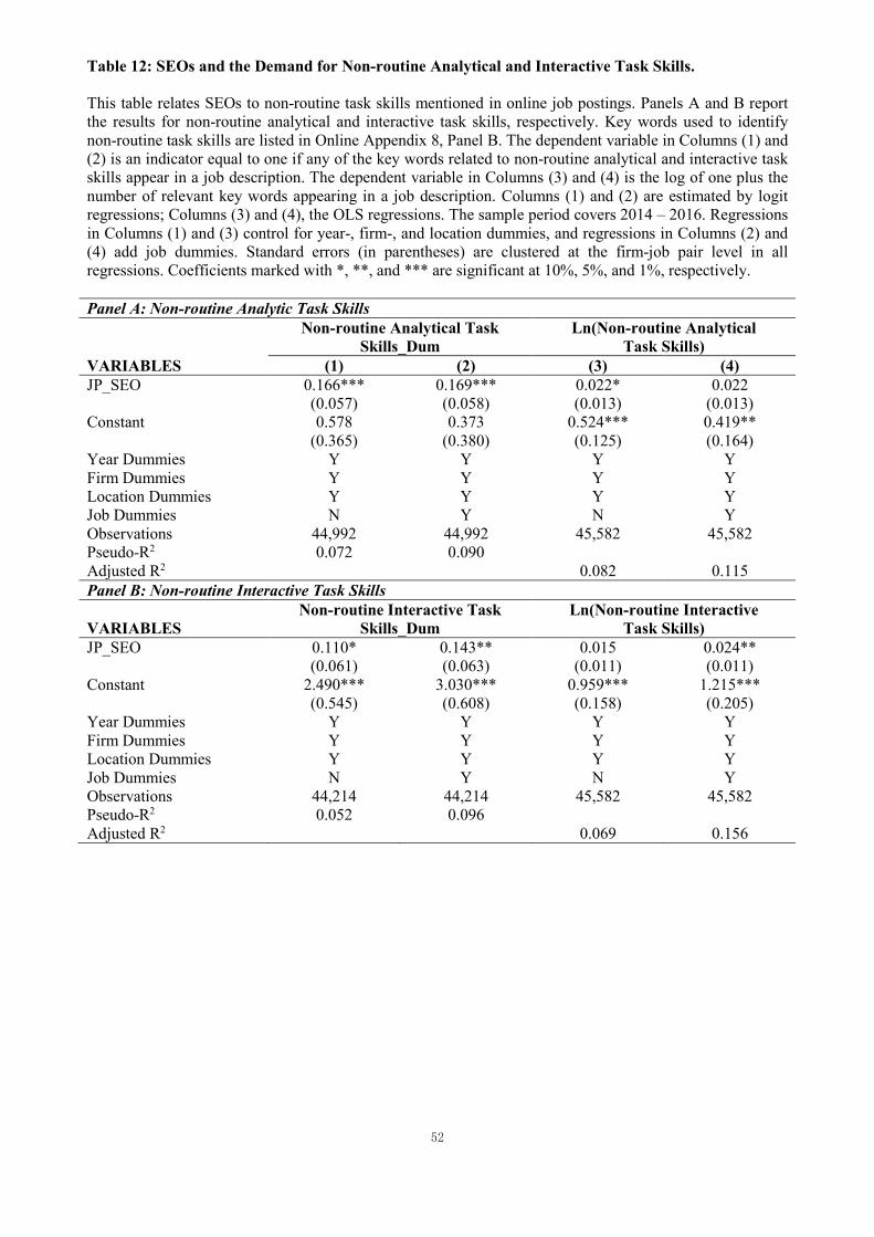
52
Table 12: SEOs and the Demand for Non-routine Analytical and Interactive Task Skills. This table relates SEOs to non-routine task skills mentioned in online job postings. Panels A and B report the results for non-routine analytical and interactive task skills, respectively. Key words used to identify non-routine task skills are listed in Online Appendix 8, Panel B. The dependent variable in Columns (1) and (2) is an indicator equal to one if any of the key words related to non-routine analytical and interactive task skills appear in a job description. The dependent variable in Columns (3) and (4) is the log of one plus the number of relevant key words appearing in a job description. Columns (1) and (2) are estimated by logit regressions; Columns (3) and (4), the OLS regressions. The sample period covers 2014 – 2016. Regressions in Columns (1) and (3) control for year-, firm-, and location dummies, and regressions in Columns (2) and (4) add job dummies. Standard errors (in parentheses) are clustered at the firm-job pair level in all regressions. Coefficients marked with *, **, and *** are significant at 10%, 5%, and 1%, respectively. Panel A: Non-routine Analytic Task Skills
Non-routine Analytical Task Skills_Dum
Ln(Non-routine Analytical Task Skills)
VARIABLES (1) (2) (3) (4) JP_SEO 0.166*** 0.169*** 0.022* 0.022
(0.057) (0.058) (0.013) (0.013)
Constant 0.578 0.373 0.524*** 0.419**
(0.365) (0.380) (0.125) (0.164)
Year Dummies Y Y Y Y Firm Dummies Y Y Y Y Location Dummies Y Y Y Y Job Dummies N Y N Y Observations 44,992 44,992 45,582 45,582 Pseudo-R2 0.072 0.090
Adjusted R2 0.082 0.115 Panel B: Non-routine Interactive Task Skills
VARIABLES Non-routine Interactive Task
Skills_Dum Ln(Non-routine Interactive
Task Skills) JP_SEO 0.110* 0.143** 0.015 0.024**
(0.061) (0.063) (0.011) (0.011)
Constant 2.490*** 3.030*** 0.959*** 1.215***
(0.545) (0.608) (0.158) (0.205)
Year Dummies Y Y Y Y Firm Dummies Y Y Y Y Location Dummies Y Y Y Y Job Dummies N Y N Y Observations 44,214 44,214 45,582 45,582 Pseudo-R2 0.052 0.096
Adjusted R2 0.069 0.156

1
Online Appendices to:
How Do Equity Offerings Affect Technology Adoption, Employees and Firm Performance?
E. Han Kim, Heuijung Kim, Yuan Li, Yao Lu, and Xinzheng Shi
2
Appendix 1: Institutional Backgrounds on Chinese Labor and Capital Markets
1. Economic Reforms and Labor Markets
China’s labor market has undergone several major changes. In the early years of Communist
China (1952-1978), the state sector dominated employment in the urban area and management did not
have the authority to hire or fire workers without government approval (Lin, Cai, and Li, 1996). Firms
set wages according to a grid determined by the government; wages barely reflected differences in
productivity (Cai, Park, and Zhao, 2008).
China embarked on economic reforms in 1978, leading to a new, floating wage system by the
mid-1980s. The reforms allowed an enterprise’s total payroll to reflect its performance in the previous
three years. (Prior to this reform, central and local planners had determined the total payroll for each
enterprise (Yueh, 2004)). At the same time, the State Council formally introduced the concept of labor
contracts, giving management the flexibility to adjust employment in response to market competition
(Meng, 2000). The labor contract system gave firms the freedom to hire suitable workers; however,
the dismissal of workers remained under the government’s tight control.
In 1992 state-owned enterprises (SOEs) were given more autonomy, enabling them to link the
total payroll more closely to firm performance and set their internal wage structures (Li and Zhao,
2003; Yueh, 2004). More reforms followed in 1994-1995, allowing listed SOEs to set their own
wages and encouraging enterprises to consider skills and productivity in addition to occupation and
rank in determining wages (Yueh, 2004). Some SOEs began to lay off workers, as the labor law
issued in 1994 permitted no-fault dismissal of workers in response to changing economic conditions
(Ho, 2006). A major state-sector restructuring followed, closing down or privatizing more than 80%
of SOEs (Hsieh and Song, 2015). When restructuring-affected employees left SOEs, they faced a
more market-driven re-employment process, and the previously inflexible labor market became one in
which supply and demand affected employment and wages. By the mid-2000s, China’s labor market
had become similar to those of other countries based on capitalism; labor is mobile, and enterprises
consider market conditions in making employment decisions and in setting wages (Cai, Park, and
Zhao, 2008).

3
During our sample period, China had well-established legal provisions for hours of work,
payment of wages, and employment. The standard workweek is 40 hours (eight hours per day, five
days per week). Overtime must be paid for any work exceeding the standard working hours and
cannot exceed three hours a day or 36 hours per month (Labor Law Article 41). Wages are paid on a
monthly basis, and may not be delayed without reason (Labor Law Article 50). Employees can be
fired in the middle of two fixed-term contracts (or ten years of employment),1 after which contracts
must be made open-ended. Open-ended contracts can be terminated only for causes (Gallagher et al.,
2015).
A consequence of these reforms particularly relevant to our study is the increase in returns to
education. Li, et al. (2012) show that the return to an additional year of schooling increased from 2.3
percent in 1988 to about 9 percent in 2000, and the return to college education increased from 7.4
percent in 1988 to 49.2 percent in 2009. These dramatic increases in returns to education are
attributable to the labor reforms and the fast-growing demand for skills (Zhang et al., 2005).
2. Capital Markets and SEOs in China
The modernization of Chinese capital markets began when former Premier Rongji Zhu, who
led China to join the World Trade Organization (WTO), spearheaded a series of reforms during his
tenure as vice premier and premier in 1993 – 2003. The reforms included restructuring state-owned
enterprises (SOEs) and the banking industry.2 A major theme of the reforms was to modernize capital
markets and corporate governance practices of SOEs. The modernization process sped up in 2001
when China officially joined the WTO. In January 2004, the State Council issued, “Opinions on
Promoting the Reform, Opening and Steady Growth of Capital Markets,” which sets the importance
of developing capital markets as a high-priority national strategy. 3 In response to the guiding
principles from the State Council, the CSRC implemented a number of new regulations to modernize
stock markets and improve corporate governance (http://www.china.com.cn/chinese/FI-
c/723240.htm). According to the World Bank, the modernization of stock markets, together with the
1 Contracts are subject to negotiation after the first term. 2 Economist, March 6th, 2003. http://www.economist.com/node/1623179 3 OECD report: Corporate Governance of Listed Companies in China. https://www.oecd.org/corporate/ca/corporategovernanceprinciples/48444985.pdf

4
rapid growth of China’s economy, have helped stock markets in mainland China to become the
second largest in the world in both market cap and total value of shares traded in 2009.4
In China, the stock market has been a more important source of external financing than the
corporate bond market, which has been growing at a much slower pace than the stock market.
Although a regulated bond market for enterprises began in 1996, regulators have allowed only very
large and stable companies to issue bonds because of the strict approval process required for issuing
bonds. Over the period 2010 through 2012, for example, China-listed firms raised 2,147.5 billion
RMB through stock markets (via SEOs and IPOs), while bond markets helped raise only 429.5 billion
RMB. Over the same period, adjusted for differences in stock market capitalization, non-financial
Chinese firms issued SEOs three times more than their U.S. counterparts did.5
The Chinese stock market is well suited to study SEOs. The types of SEOs available and the
underwriting procedures in China are similar to those in the U.S. There are three types of SEOs: rights
offerings, underwritten offerings, and private placements to no more than ten qualified investors. As
in the U.S., there are two types of underwriting contracts, best efforts and firm commitments.
In comparison to U.S. SEOs, Chinese SEOs provide a cleaner sample to study how firms use
the proceeds from SEOs because virtually all Chinese SEOs are primary shares.6 SEOs in the U.S.
often include secondary offerings, sale of shares held by insiders and block holders. Proceeds of
secondary offerings do not go to the firm and hence cannot affect investment and employment
decisions. Thus, if one studies the effects of deploying U.S. SEO proceeds without carefully screening
out secondary offerings, the results will be noisy.
4http://data.worldbank.org/indicator/CM.MKT.LCAP.CD?end=2016&locations=CN-JP-US-HK-FR-GB-DE&name_desc=false&page=5&start=2003&view=chart. 5 Over the period of 2010 through 2012, the average total Chinese stock market capitalization is 3,949.77 billion USD and non-financial Chinese listed firms raised 86.09 billion USD through SEOs, or 2.18% of total market capitalization. This is more than three times of the ratio for US counterparts. During the same period, the average market capitalization of the US stock market is 17,149.34 billion USD and non-financial US listed firms raised 102.75 billion USD through SEOs, or 0.6% of the total market cap. Total stock market capitalization excludes financial firms. Capital raised through SEOs is taken from SDC Platinum. The market capitalization data are taken from the data on the World Bank website (http://data.worldbank.org/). Capital raised through SEOs includes proceeds only from primary offerings. 6 There were only three mixed offerings containing secondary offerings of state-owned shares, all of which occurred in 2001. At that time, the CSRC required that if a firm plans to issue N new shares through an underwritten offering and has state-owned shares, then the offering must contain 10% of N state-owned shares. The regulation lasted only four months, and there have been no mixed offerings since 2001.

5
References
Cai, Fang, Albert Park and Yaohui Zhao, 2008, The Chinese Labor Market in the Reform Era in China’s Great Economic Transformation, In: Brandt L. Rawski T (Ed.), The Chinese Labor Market in the Reform Era, Cambridge: Cambridge University Press, Chapter 6, 167-214.
Gallagher, Mary, John Giles, Albert Park and Meiyan Wang, 2015, China’s 2008 Labor Contract Law: Implementation and Impacts on Workers, Human Relations 68, 197-235.
Ho, Virginia, 2006, Labor Law Era in China’s Reform Era: The Evolving Legal Framework for Labor Rights, Unpublished Manuscript.
Hsieh, Chang-Tai and Zheng (Michael) Song, 2015, Grasp the Large, Let Go of the Small: The Transformation of the State Sector in China, Brookings Papers on Economic Activity Spring, 295-346.
Li, Hongbin, Lei Li, Binzhen Wu and Yanyan Xiong, 2012, The End of Cheap Chinese Labor, Journal of Economic Perspectives 26, 57-74.
Li, Shi and Yaohui Zhao, 2003, The Decline of In-kind Wage Payments in Urban China, Journal of Chinese Economics and Business Studies 1, 245-258.
Lin, Justin Yifu, Fang Cai and Zhou Li, 1996, The China Miracle: Development Strategy and Economic Reform, Hong Kong Chinese University Press.
Meng, Xin, 2000, Labor Market Reform in China, Cambridge and New York: Cambridge University Press.
Yueh, Linda, 2004, Wage Reforms in China during the 1990s, Asian Economic Journal 18, 149-164. Zhang, Junsen, Yaohui Zhao, Albert Park, and Xiaoqing Song, 2005, Economic Returns to Schooling
in Urban China, 1988 to 2001, Journal of Comparative Economics 33, 730-752.

6
Appendix 2: Construction of the Instrumental Variable. This table illustrates how the instrument, SEOIneligible, is constructed. “Conditions” specify the past three-year period during which the minimum payout ratio applies to make a firm ineligible to issue a public SEO. For example, 2003 – 2005 < 20% means that if the payout ratio over 2003 – 2005 is less than 20%, the firm is ineligible to issue a public SEO in 2006. In this table, we assume it takes two years to complete an SEO. Since SEO years include the SEO year and two post-SEO years, we turn on the instrument in 2008, 2009, and 2010 for firms affected by the 2006 regulation in 2006. We follow the same procedure for firms affected by the 2006 regulation in 2007, and for firms affected by the 2008 regulation in 2008 and 2009. The CSRC specifies the formula for the payout ratio as (Dt-1 + Dt-2 + Dt-3) / [(It-1 + It-2+ It-3) / 3], where Dt is the amount of dividends paid in year t and It is the amount of distributable profits in year t as measured by net income (the parent’s net income for consolidated financial statements. For firms listed for less than three years, the same formula (with fewer years) applies to the years they have been listed. Dt includes stock dividends when calculating the ratio for the 2006 regulation, but only cash dividends when calculating the 2008 regulation ratio. Year SEOIneligible Conditions 2000 0 NA 2001 0 NA 2002 0 NA 2003 0 NA 2004 0 NA 2005 0 NA 2006 0 NA 2007 0 NA 2008 1 If 2003 – 2005 < 20% 2009 1 If 2004 – 2006 < 20% or 2003 – 2005 < 20% 2010 1 If 2005 – 2007 < 30%, 2004 – 2006 < 20%, or 2003 – 2005 < 20% 2011 1 If 2006 – 2008 < 30%, 2005 – 2007 < 30%, or 2004 – 2006 < 20% 2012 1 If 2006 – 2008 < 30% or 2005 – 2007 < 30%

7
Appendix 3: Variable Definitions and Data Sources. Variables
Definition
Data Sources
SEO-related Variables SEO An indicator equal to one in SEO years (the year in which SEO proceeds are received and the two years after), and zero otherwise. It applies to only public offerings.
CSMAR
SEOIneligible Instrument for SEO years. Online Appendix 2 illustrates how it is constructed. Wind
JP_SEO An indicator equal to one in the year in which a firm receives SEO (public or private placement) proceeds, and zero otherwise.
CSMAR
Outcome Variables EMP The total number of employees at the firm-level Unit: 100. Resset
Production The number of production workers. Resset Staff The number of support staff. Resset Tech_R&D The number of technicians (including engineers and IT
staff) and R&D employees. Resset
S&M The number of employees in sales and marketing. Resset Finance The number of accounting and finance staff. Resset Others The number of employees with unidentified occupation. Resset BA The number of employees with four-year university
bachelor’s degrees and above. Resset
NBA The number of employees without four-year university bachelor’s degrees. Resset
Grad The number of employees with post-graduate degrees. Resset Fixed_Tech
Expenditures on machines and equipment in 2000 RMB. Unit: 1,000,000.
CSMAR
Intangible_Tech Expenditures on technology-related intangible assets in 2000 RMB. Unit: 10,000.
CSMAR
Capex Total capital expenditures in 2000 RMB. Unit: 1,000,000.
Resset
ROA Return on assets: Net income divided by total assets. Resset SALES_GR Sales growth rate from year t-1 to year t. Resset SALES/Employees Total sales in 2000 RMB (Unit: 1,000,000) divided by
the total number of employees. Resset
TFP
The residuals of ln(Y) = ai + at + ln(total assets) + ln(EMP) + eit. Y is s total output, as measured by prime operating revenue + changes in inventory* the cost profit margin, where the cost profit margin = prime operating revenue /cost of goods sold. ai is firm fixed effects and at is year fixed effects.
Resset
AWAGE Total annual cash salary and bonuses to all employees in 2000 RMB divided by total number of employees. Unit: 10,000.
Resset
AWAGE_NonEXE AWAGE for all non-executive employees. Unit: 10,000. Resset AEXEPAY AWAGE for all executives. Unit: 10,000. Resset Payroll Total annual cash salary and bonuses to all employees in
2000 RMB. Unit: 1,000,000. Resset
Payroll_NonExe Payroll to all non-executive employees in 2000 RMB. Unit: 1,000,000. Resset
Payroll_Exe Payroll to all executives in 2000 RMB. Unit: 1,000,000. Resset

8
Outcome Variables
Definition
Data Sources
Adv_Computer_Dum An indicator for the presence of words indicating advanced computer skills in a job advertisement. Lagou.com
Basic_Computer_Dum An indicator for the presence of words indicating basic computer skills in a job advertisement. Lagou.com
Adv_Computer The number of words indicating advanced computer skills in a job advertisement. Lagou.com
Basic_Computer The number of words indicating advanced computer skills in a job advertisement. Lagou.com
Non-routine Analytical Task Skill_Dum
An indicator for the presence of words indicating non-routine analytical task skills in a job advertisement. Lagou.com
Non-routine Analytical Task Skills
The number of words indicating non-routine analytical task skills in a job advertisement. Lagou.com
Non-routine Interactive Task Skill_Dum
An indicator for the presence of words indicating non-routine interactive task skills in a job advertisement. Lagou.com
Non-routine Interactive Task Skills
The number of words indicating non-routine interactive task skills in a job advertisement. Lagou.com
Control Variables P3_PR
The payout ratio during the most recent past three years as defined by the CSRC. See Section 3.2.3. If it is negative, we replace it by one.
Resset
P3_PR_D
Indicator equal to one if the payout ratio during the most recent past three years as defined by the CSRC is negative, zero otherwise.
Resset
NYEAR_LISTED The number of years a firm has been listed since its IPO. Resset MIN_WAGE The minimum monthly wage in the province or
provincial city of the firm’s headquarters location in 2000 RMB.
Government Websites
LAWSCORE An index for the strength of legal environment described in Section 3.2.3. The index is updated by the National Economic Research Institute up to 2009. For years after 2009, we use the 2009 index.
National Economic Research Institute
Labor_Law_Effect The degree to which the 2008 Labor Law of People’s Republic of China affects a firm. See Section 3.2.3. CSMAR
SALES Total sales in 2000 RMB. Unit: 1,000,000. Resset %_LARGEST_SH The percentage of shares held by the largest shareholder. Resset DIV_PR Dividend payout ratio, equal to total dividend paid over
net income. Resset
%_STATE_OWN The percentage of shares held by the local or central
government. Resset
%_IND_DIR The percentage of independent directors on the board. Resset %_NONTRD_SH The percentage of non-tradable shares. Resset Leverage Total liability divided by total assets. Resset PPE/TA Property, plants, and equipment divided by total assets. Resset Affected An indicator for firms affected by the 2006 regulation. Resset

9
Appendix 4: The First-stage Regression Results. This table reports the first-stage estimation results: Column (1) is for the second-stage results reported in Tables 3 – 8 and Online Appendix 8. Columns (2) - (5) are for the second-stage results reported in Table 10, Columns (2) - (5), respectively. The first-stage is estimated by the firm- level conditional logistic regression. Online Appendix 3 provides variable definitions and data sources. The sample period covers 2000 – 2012. Robust standard errors clustered at the firm level are in parentheses. Coefficients marked with *, **, and *** are significant at 10%, 5%, and 1%, respectively.
SEO
VARIABLES (1) (2) (3) (4) (5) SEOIneligible -1.434*** -1.616*** -1.067*** -1.352*** -1.370***
(0.371) (0.404) (0.350) (0.471) (0.364)
P3_PR 0.120 0.126 0.093 0.108 0.091
(0.089) (0.089) (0.089) (0.089) (0.088)
P3_PR_D -1.003*** -0.999*** -0.993*** -0.976*** -0.911***
(0.362) (0.363) (0.358) (0.359) (0.340)
Ln(NYEAR_LISTED) 4.430*** 4.438*** 4.448*** 4.508*** 4.251***
(0.462) (0.462) (0.463) (0.461) (0.455)
Ln(SALES) 1.033*** 1.041*** 1.018*** 1.010*** 1.022***
(0.170) (0.170) (0.169) (0.166) (0.163)
Leverage -5.225*** -5.275*** -5.142*** -5.026*** -5.000***
(0.810) (0.809) (0.810) (0.794) (0.788)
PPE/TA 1.287 1.309 1.293 1.281 1.370
(0.941) (0.944) (0.935) (0.918) (0.918)
%_IND_DIR -0.792 -0.821 -0.828 -0.786 -0.825
(0.636) (0.635) (0.634) (0.640) (0.639)
%_STATE_OWN 0.254 0.256 0.218 0.167 0.196
(0.523) (0.522) (0.520) (0.519) (0.514)
%_LARGEST_SH -2.308** -2.303** -2.325** -2.342** -1.926*
(1.137) (1.146) (1.131) (1.120) (1.095)
%_NONTRD_SH -1.552*** -1.561*** -1.522** -1.551*** -1.353**
(0.601) (0.601) (0.601) (0.601) (0.589)
DIV_PR 0.108 0.107 0.100 0.100 0.107
(0.075) (0.073) (0.074) (0.075) (0.074)
Ln(MIN_WAGE) 1.690** 1.734** 1.605** 1.604** 1.574**
(0.677) (0.676) (0.673) (0.670) (0.683)
LAWSCORE 0.064 0.064 0.069 0.069 0.062
(0.068) (0.068) (0.068) (0.068) (0.069)
Labor_Law_Effect 0.115 0.119 0.102 0.107 0.111
(0.084) (0.085) (0.082) (0.082) (0.081)
Year Dummies Y Y Y Y Y Observations 5,251 5,251 5,251 5,251 5,251 Pseudo R2 0.4153 0.4167 0.4127 0.4126 0.397 Wald 635.3 633.3 643.7 646.4 602.3

10
Appendix 5: OLS Estimation on Firm-level Employment. This table reports the OLS estimates of the impacts that SEOs have on firm-level employment. The dependent variable in Column (1) is the log of the total number of employees; dependent variables in the remaining columns are the log of one plus the number of employees in each occupation or education category. All regressions include firm- and year fixed effects. Online Appendix 3 provides variable definitions and data sources. The sample period covers 2000 – 2012. Robust standard errors are reported in parentheses. Coefficients marked with *, **, and *** are significant at 10%, 5%, and 1%, respectively.
Ln Ln Ln Ln Ln Ln Ln Ln Ln Ln
(EMP) (Production) (Staff) (Tech_R&D) (S&M) (Finance) (Others) (Grad) (BA) (NBA)
VARIABLES (1) (2) (3) (4) (5) (6) (7) (8) (9) (10) SEO -0.028* -0.069* 0.010 0.022 -0.012 -0.012 -0.116 -0.009 0.028 -0.004
(0.017) (0.037) (0.042) (0.023) (0.028) (0.017) (0.082) (0.034) (0.023) (0.025)
P3_PR 0.010* 0.041*** 0.032** 0.004 0.018 -0.004 -0.031 -0.020 0.018** 0.011
(0.006) (0.013) (0.015) (0.008) (0.011) (0.007) (0.030) (0.012) (0.009) (0.008)
P3_PR_D -0.013 -0.016 0.087 -0.069** 0.028 -0.036 0.050 -0.080* -0.078** 0.008
(0.024) (0.055) (0.060) (0.033) (0.041) (0.026) (0.120) (0.046) (0.033) (0.032)
Ln(NYEAR_LISTED) 0.093*** 0.063* -0.005 0.112*** 0.112*** 0.073*** 0.441*** 0.079*** 0.052** 0.073***
(0.015) (0.036) (0.039) (0.024) (0.030) (0.019) (0.074) (0.029) (0.022) (0.021)
Ln(MIN_WAGE) -0.272*** -0.194* -0.249** -0.217*** -0.096 -0.159*** 0.032 0.263** -0.002 -0.445***
(0.051) (0.116) (0.125) (0.075) (0.094) (0.056) (0.248) (0.112) (0.082) (0.075)
LAWSCORE -0.013*** 0.009 0.001 0.004 0.015 -0.011** -0.069*** -0.021** -0.009 -0.025***
(0.005) (0.011) (0.011) (0.007) (0.009) (0.005) (0.021) (0.010) (0.007) (0.008)
Labor_Law_Effect -0.004 -0.042*** 0.010 0.006 -0.024** 0.002 0.051*** -0.036*** -0.020*** 0.011**
(0.004) (0.008) (0.009) (0.006) (0.010) (0.004) (0.016) (0.006) (0.005) (0.005)
Ln(SALES) 0.418*** 0.317*** 0.239*** 0.401*** 0.420*** 0.320*** 0.325*** 0.397*** 0.420*** 0.439***
(0.011) (0.022) (0.021) (0.016) (0.022) (0.011) (0.040) (0.020) (0.016) (0.017)
%_LARGEST_SH -0.083 -0.241 0.303** 0.006 0.069 0.129* 0.090 -0.107 0.074 -0.324***
(0.075) (0.156) (0.148) (0.108) (0.138) (0.078) (0.295) (0.143) (0.107) (0.112)
DIV_PR 0.004*** 0.008*** 0.006*** 0.002** -0.002** 0.003*** -0.004 -0.001 0.005*** 0.005***
(0.001) (0.001) (0.002) (0.001) (0.001) (0.001) (0.003) (0.015) (0.001) (0.000)
%_STATE_OWN 0.123*** 0.003 0.066 0.077 -0.006 0.061* 0.220 0.025 0.149*** 0.140***
(0.030) (0.069) (0.074) (0.050) (0.064) (0.033) (0.136) (0.050) (0.045) (0.042)
%_IND_DIR 0.040 -0.187 -0.017 0.223*** 0.188** 0.077 0.138 0.026 0.028 0.073
(0.051) (0.116) (0.128) (0.072) (0.094) (0.054) (0.243) (0.109) (0.080) (0.078)
%_NONTRD_SH 0.038 0.042 -0.091 -0.078 -0.059 -0.014 0.013 -0.018 -0.033 0.043
(0.043) (0.090) (0.096) (0.058) (0.073) (0.042) (0.198) (0.084) (0.061) (0.063)
Leverage 0.277*** -0.084 0.394*** 0.180*** 0.171* 0.424*** 0.571*** 0.199** 0.273*** 0.284***
(0.048) (0.098) (0.100) (0.067) (0.095) (0.048) (0.194) (0.093) (0.068) (0.067)
PPE/TA 0.523*** 0.944*** 0.413*** 0.281*** -0.225** -0.077 -0.504** -0.049 0.177** 0.687***
(0.057) (0.111) (0.112) (0.080) (0.112) (0.058) (0.218) (0.110) (0.081) (0.089)
Constant 1.517*** 5.148*** 3.431*** 3.977*** 2.685*** 2.381*** 1.165 -1.456** 2.147*** 6.805***
(0.319) (0.712) (0.759) (0.460) (0.588) (0.341) (1.502) (0.694) (0.504) (0.474)
Firm & Year FE Y Y Y Y Y Y Y Y Y Y Observations 16,964 16,964 16,964 13,916 10,576 13,326 16,964 8,109 11,650 11,650 R-squared 0.884 0.747 0.552 0.803 0.843 0.842 0.518 0.896 0.873 0.902

11
Appendix 6: Alternative Measures of TFP. This table reports the second-stage estimation of the impacts that SEOs have on the alternative measures of TFPs. TFP_A1 is the residuals from ln(Y) = ai + at + ln(total assets) + ln(total payrolls) + eit. TFP_A2 is the residuals from ln(Y) = ai + at + ln(total assets) + ln(total number of production workers) + eit. Y is total output, as measured by prime operating revenue + changes in inventory* the cost profit margin, where the cost profit margin = prime operating revenue / cost of goods sold. ai is firm fixed effects and at is year fixed effects. Online Appendix 3 provides variable definitions and data sources. The sample period covers 2000 – 2012. Bootstrapped standard errors are reported in parentheses. Coefficients marked with *, **, and *** are significant at 10%, 5%, and 1%, respectively.
TFP_A1 TFP_A2
VARIABLES (1) (2) SEO� 0.049* 0.096***
(0.028) (0.026)
P3_PR -0.010*** -0.001
(0.004) (0.003)
P3_PR_D -0.044*** -0.026
(0.012) (0.019)
Ln(NYEAR_LISTED) -0.103*** -0.083***
(0.014) (0.011)
Ln(MIN_WAGE) -0.006 -0.004
(0.032) (0.030)
LAWSCORE 0.003 -0.010***
(0.003) (0.003)
Labor_Law_Effect 0.000 -0.003
(0.002) (0.003)
Ln(SALES) 0.308*** 0.402***
(0.008) (0.008)
%_LARGEST_SH -0.013 -0.040
(0.045) (0.054)
DIV_PR -0.004 -0.003
(0.007) (0.009)
%_STATE_OWN -0.144*** -0.090***
(0.018) (0.017)
%_IND_DIR -0.051 -0.029
(0.032) (0.032)
%_NONTRD_SH -0.003 0.037
(0.030) (0.032)
Leverage -0.159*** -0.288***
(0.040) (0.039)
PPE/TA -0.283*** -0.110***
(0.037) (0.038)
Constant -1.539*** -2.143***
(0.198) (0.187)
Firm & Year FE Y Y Observations 16,981 16,827

12
Appendix 7: Average Annual Wages in China by Education and Occupation. This table reports average annual wages in China by education or occupation. The data is from China Urban Household Survey (2000-2009), which provides access to nine provinces; Beijing, Liaoning, Zhejiang, Anhui, Hubei, Guangdong, Sichuan, Shaanxi, and Gansu. Annual wage is deflated using provincial CPI with 2000 as the base year. The unit is Chinese RMB.
Education Occupation
Year College or above High School Middle School or
below Technician Production Workers
Staff or Service Workers
Agricultural Workers Others
2000 11084.013 8944.776 5139.363 15239.261 9258.860 11053.963 8566.029 7946.278 2001 11976.958 9554.838 5438.288 16852.991 9864.254 11841.001 9827.922 8882.542 2002 15822.367 10409.411 5757.975 18404.414 10912.095 13807.288 9452.208 9661.626 2003 17728.367 11346.542 5975.318 20489.257 12303.120 15216.043 10937.459 11118.318 2004 19451.303 12139.160 6495.877 23086.913 13622.273 16191.782 12360.412 12257.059 2005 21261.428 13013.126 7123.790 25598.902 14743.270 18072.238 15012.060 14361.187 2006 23030.351 14092.422 7931.302 27949.907 16697.195 19682.444 16756.711 15198.924 2007 24665.948 15261.617 8603.666 29624.443 17833.485 21563.516 18206.153 17030.791 2008 27924.529 16415.125 9329.643 32551.162 20094.639 23523.721 19247.500 20093.954 2009 30928.259 18155.407 10323.152 35799.283 22402.561 26124.442 23231.018 20988.433

13
Appendix 8: Online Job Posting Sample and Words Related to Skills. This table provides information obtained from job posting data. Panel A reports the number of full-time job advertisements in Lagou.com (https://www.lagou.com) posted by firms listed on Shanghai and Shenzhen Stock Exchanges over 2014 - 2016. Panel A, Column (1) shows the number of all new full-time job advertisements by year, and Column (2) shows the number of new full-time job advertisements in the year in which firms issued seasoned equity offerings (including underwritten offerings, rights offerings, and private placements). Duplicated advertisements are excluded. Panel B provides the list of key words used to identify the requirements for the different types of skills. The key words are the English translation of Chinese words mentioned in job advertisements. Panel A: Sample Distribution
Year Number of Unique Job Advertisements JP_SEO=1
(1) (2)
2014 5,702 1,410 2015 15,041 3,591 2016 24,842 2,790 Total 45,585 7,791
Panel B: Key Words Used to Identify Different Skill Requirements Skills Key Words Advanced computer
Programming, Java, SQL, Python, developing, server, artificial intelligence, big data, machine learning, html, and software
Basic computer Diannao (an unofficial name of computer), Computer, PPT, presentation slides, Excel, spreadsheets, Microsoft Office, Windows, and Word.
Non-routine analytical task skills
Research, analysis, problem solving, analytical critical thinking, math, statistics, learning, thinking, changing, improving, professional writing, and reporting.
Non-routine interactive task skills
Communication, cooperation, negotiation, services, clients, persuading, selling, management, monitoring, supervisory, leadership, mentoring, guidance, and making a deal.
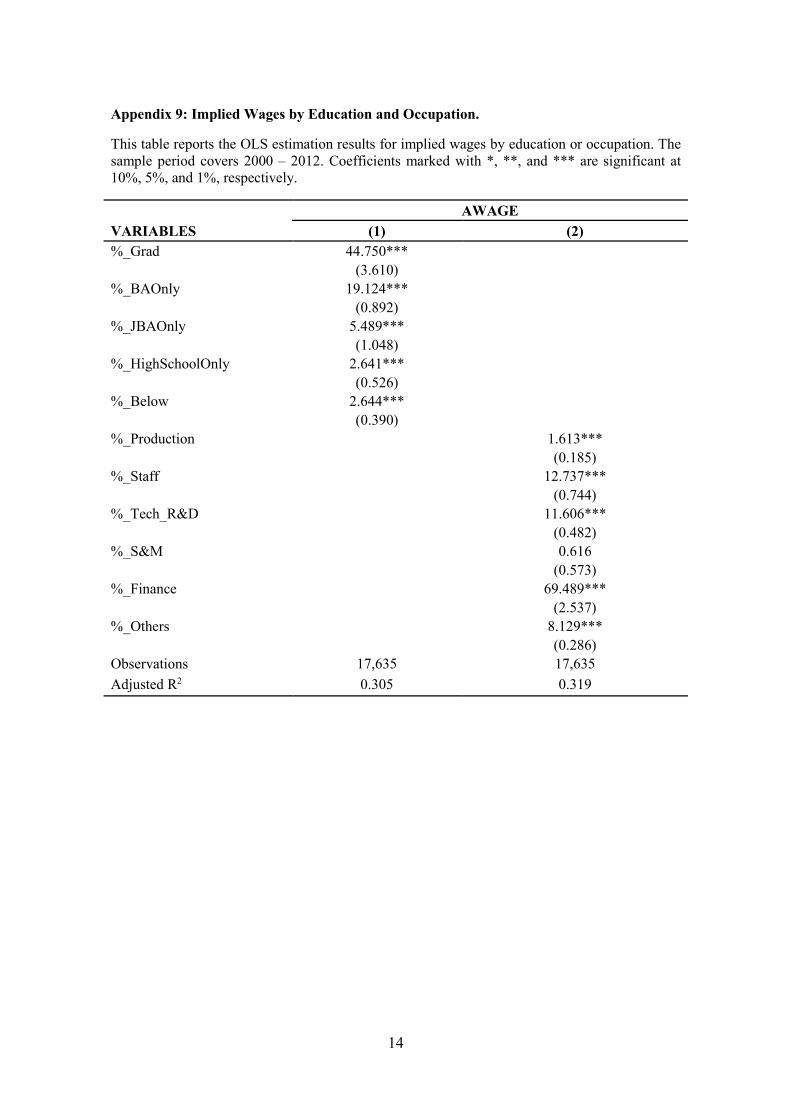
14
Appendix 9: Implied Wages by Education and Occupation.
This table reports the OLS estimation results for implied wages by education or occupation. The sample period covers 2000 – 2012. Coefficients marked with *, **, and *** are significant at 10%, 5%, and 1%, respectively.
AWAGE
VARIABLES (1) (2) %_Grad 44.750***
(3.610) %_BAOnly 19.124***
(0.892)
%_JBAOnly 5.489***
(1.048)
%_HighSchoolOnly 2.641***
(0.526)
%_Below 2.644***
(0.390)
%_Production
1.613***
(0.185)
%_Staff
12.737***
(0.744)
%_Tech_R&D
11.606***
(0.482)
%_S&M
0.616
(0.573)
%_Finance
69.489***
(2.537)
%_Others
8.129***
(0.286)
Observations 17,635 17,635 Adjusted R2 0.305 0.319