how does a dictation machine recognize speech?

Chapter 4

How does a dictation machine recognize speech?

This Chapter is not about how to wreck a nice beach45

T. Dutoit (°), L. Couvreur (°), H. Bourlard (*)

(°) Faculté Polytechnique de Mons, Belgium

(*) Ecole Polytechnique Fédérale de Lausanne, Switzerland

There is magic (or is it witchcraft?) in a speech recognizer that transcribes

continuous radio speech into text with a word accuracy of even not more

than 50%. The extreme difficulty of this task, tough, is usually not

perceived by the general public. This is because we are almost deaf to the

infinite acoustic variations that accompany the production of vocal sounds,

which arise from physiological constraints (co-articulation), but also from

the acoustic environment (additive or convolutional noise, Lombard

effect), or from the emotional state of the speaker (voice quality, speaking

rate, hesitations, etc.)46. Our consciousness of speech is indeed not

stimulated until after it has been processed by our brain to make it appear

as a sequence of meaningful units: phonemes and words.

In this Chapter we will see how statistical pattern recognition and

statistical sequence recognition techniques are currently used for trying to

mimic this extraordinary faculty of our mind (4.1). We will follow, in

Section 4.2, with a MATLAB-based proof of concept of word-based

automatic speech recognition (ASR) based on Hidden Markov Models

(HMM), using a bigram model for modeling (syntactic-semantic) language

constraints.

45 It is, indeed, about how to recognize speech. 46 Not to mention inter-speaker variability, nor regional dialects.

104 T. Dutoit, L. Couvreur, H. Bourlard

4.1 Background – Statistical Pattern Recognition

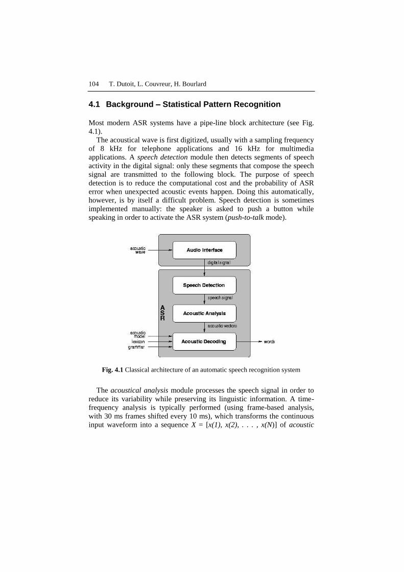
Most modern ASR systems have a pipe-line block architecture (see Fig.

4.1).

The acoustical wave is first digitized, usually with a sampling frequency

of 8 kHz for telephone applications and 16 kHz for multimedia

applications. A speech detection module then detects segments of speech

activity in the digital signal: only these segments that compose the speech

signal are transmitted to the following block. The purpose of speech

detection is to reduce the computational cost and the probability of ASR

error when unexpected acoustic events happen. Doing this automatically,

however, is by itself a difficult problem. Speech detection is sometimes

implemented manually: the speaker is asked to push a button while

speaking in order to activate the ASR system (push-to-talk mode).

Fig. 4.1 Classical architecture of an automatic speech recognition system

The acoustical analysis module processes the speech signal in order to

reduce its variability while preserving its linguistic information. A time-

frequency analysis is typically performed (using frame-based analysis,

with 30 ms frames shifted every 10 ms), which transforms the continuous

input waveform into a sequence X = [x(1), x(2), . . . , x(N)] of acoustic

How does a dictation machine recognize speech? 105

feature vectors x(n)47. The performances of ASR systems (in particular,

their robustness, i.e. their resistance to noise) are very much dependent on

this formatting of the acoustic observations. Various types of feature

vectors can be used, such as the LPC coefficients described in Chapter 1,

although specific feature vectors, such as the Linear Prediction Cepstral

Coefficients (LPCC) or the Mel Frequency Cepstral Coefficients (MFCC;

Picone 1993), have been developed in practice for speech recognition,

which are somehow related to LPC coefficients.

The acoustic decoding module is the heart of the ASR system. During a

training phase, the ASR system is presented with several examples of

every possible word, as defined by the lexicon. A statistical model (4.1.1)

is then computed for every word such that it models the distribution of the

acoustic vectors. Repeating the estimation for all the words, we finally

obtain a set of statistical models, the so-called acoustic model, which is

stored in the ASR system. At run-time, the acoustic decoding module

searches the sequence of words whose corresponding sequence of models

is the “closest” to the observed sequence of acoustic feature vectors. This

search is complex since neither the number of words, nor their

segmentation, are known in advance. Efficient decoding algorithms

constrain the search for the best sequence of words by a grammar, which

defines the authorized, or at least the most likely, sequence of words. It is

usually described in terms of a statistical model: the language model.

In large vocabulary ASR systems, it is hard if not impossible to train

separate statistical models for all words (and even to gather the speech data

that would be required to properly train a word-based acoustic model). In

such systems, words are described as sequences of phonemes in a

pronunciation lexicon, and statistical modeling is applied to phonemic

units. Word-based models are then obtained by concatenating the

phoneme-based models. Small vocabulary systems (<50 words), on the

contrary, usually consider words as basic acoustic units and therefore do

not require a pronunciation lexicon.

4.1.1 The statistical formalism of ASR

The most common statistical formalism of ASR48, which we will use

throughout this Chapter, aims to produce the most probable word sequence

47 Although x(n) is a vector, it will not be written with a bold font in this Chapter,

to avoid overloading all equations. 48 There are numerous textbooks that explain these notions in detail. See for

instance (Gold and Morgan 2000), (Bourlard and Morgan 1994) or (Bourlard


W* given the acoustic observation sequence X. This can be expressed

mathematically by the so-called Bayesian, or Maximum a Posteriori

(MAP) decision rule as:

* arg max ( | , )i

iW

W P W X (4.1)49

where Wi represents the i-th possible word sequence and the conditional

probability is evaluated over all possible word sequences50, and

represents the set of parameters used to estimate the probability

distribution.

Since each word sequence Wi may be realized as an infinite number of

possible acoustic realizations, it is represented by its model M(Wi), also

written Mi for the sake of simplicity, which is assumed to be able to

produce all such possible acoustic realizations. This yields:

* arg max ( | , )i

iM

M P M X (4.2)

where M* is (the model of) the sequence of words representing the

linguistic message in input speech X, Mi is (the model of) a possible word

sequence Wi, P(Mi | X,) is the posterior probability of (the model of) a

word sequence given the acoustic input X, and the maximum is evaluated

over all possible models (i.e., all possible word sequences).

Bayes‟ rule can be the applied to (4.2), yielding:

( | , ) ( | )( | , )

( | )

i ii

P X M P MP M X

P X

(4.3)

2007). For a more general introduction to pattern recognition, see also (Polikar

2006) or the more complete (Duda et al. 2000). 49 In equation (4.1), Wi and X are not random variables: they are values

taken by their respective random variables. As a matter of fact, we will often use

in this Chapter a shortcut notation for probabilities, when this does not bring

confusion. The probability P(A=a|B=b) that a discrete random variable A takes

value a given the fact that random variable B takes value b will simply be

written P(a|b). What is more, we will use the same notation when A is a

continuous random variable for referring to probability density pA|B=b (a)). 50 It is assumed here that the number of possible word sequences is finite,

which is not true for natural languages. In practice, a specific component of the

ASR, the decoder, takes care of this problem by restricting the computation of

(4.1) for a limited number of most probable sequences.


where ( | , )iP X M represents the contribution of the so-called acoustic

model (i.e., the likelihood that a specific model Mi has produced the

acoustic observation X), ( | )iP M represents the contribution of the so-

called language model (i.e., the a priori probability of the corresponding

word sequence), and P(X| ) stands for the a priori probability of the

acoustic observation. For the sake of simplicity (and tractability of the

parameter estimation process), state-of-the-art ASR systems always

assume independence between the acoustic model parameters, which will

now be denoted A and the parameters of the language model, which will

be denoted L .

Based on the above, we thus have to address the following problems:

Decoding (recognition): Given an unknown utterance X, find the

most probable word sequence W* (i.e., the most probable word

sequence model M*) such that:

* ( | , ) ( | )arg max

( | , )i

i A i L

M A L

P X M P MM

P X

(4.4)

Since during recognition all parameters A and L are frozen,

probability ( | , )A LP X is constant for all hypotheses of word

sequences (i.e., for all choices of i) and can thus be ignored, so that

(4.4) simplifies to:

* arg max ( | , ) ( | )i

i A i LM

M P X M P M (4.5)

Acoustic modeling: Given (the model of) a word sequence, Mi,

estimate the probability ( | , )i AP X M of the unknown utterance

X.

This is typically carried out using Hidden Markov Models

(HMM; see Section 4.1.3). It requires to estimate the acoustic model

A . At training time, a large amount of training utterances Xj (j =

1,… , J) with their associated models Mj are used to estimate the

optimal acoustic parameter set *

A , such that:


*

1

1

arg max ( | , )

arg max log( ( | , ))

A

A

J

A i A

j

J

i A

j

P X M

P X M

(4.6)

which is referred to as the Maximum Likelihood (ML), or Maximum

Log Likelihood criterion51.

Language modeling: The goal of the language model is to estimate

prior probabilities of sentence models ( | )i LP M .

At training time, the language model parameters L are

commonly estimated from large text corpora. The language model is

most often formalized as word-based Markov models (See Section

4.1.2), in which case L is the set of transition probabilities of

these chains, also known as n-grams.

4.1.2 Markov models

A Markov model is the simplest form of a Stochastic Finite State

Automaton (SFSA). It describes a sequence of observations X = [x(1), x(2),

… , x(N)] as the output of a finite state automaton (Fig. 4.2) whose internal

states {q1, q2, … , qK} are univocally associated with possible observations

{x1, x2, … , xK} and whose state-to-state transitions are associated with

probabilities: a given state qk always outputs the same observation xk,

except initial and final states (qI and qF, which output nothing); the

transition probabilities from any state sum to one. The most important

constraint imposed by a (first order) Markov model is known as the

: the probability of a state (or that of the associated observation) only

depends on the previous state (or that of the associated observation).

51 Although both criteria are equivalent, it is usually more convenient to work with

the sum of log likelihoods. As a matter of fact, computing products of

probabilities (which are often significantly lower than one) quickly exceeds the

floating point arithmetic precision. Even the log of a sum of probabilities can be

estimated, when needed, using log likelihoods (i.e., without having to compute

likelihoods at any time), using:

(log log )log( ) log( ) log 1 b aa b a e


x1

x2

x3

xK

xK-1

x4

P(x1|x2)

qF

P(x2|x2)

P(x1|x1)

qI

P(xK-1|qI)

P(qF|x3)

Fig. 4.2 A typical Markov model52. The leftmost and rightmost states are the

initial and final states. Each internal state qk in the center of the figure is

associated to a specific observation xk (and is labeled as such). Transition

probabilities are associated to arcs (only a few transition probabilities are shown).

The probability of X given such a model reduces to the probability of

the sequence of states [qI, q(1), q(2), …, q(N), qF] corresponding to X, i.e.

to a product of transition probabilities (including transitions from state qI

and transitions to state qF):

2

( ) ( (1) | ) ( ( ) | ( 1)) ( | ( ))N

I F

n

P X P q q P q n q n P q q N

(4.7)

where q(n) stands for the state associated with observation x(n). Given the

one-to-one relationship between states and observations, this can also be

written as:

52 The model shown here is ergodic: transitions are possible from each state to all

other states. In practical applications (such as in ASR, for language modeling),

some transitions may be prohibited.


2

( ) ( (1)| ) ( ) | ( 1) | ( )N

n

P X P x I P x n x n P F x N

(4.8)

where I and F stand for the symbolic beginning and end of X.

The set of parameters, represented by the (K×K)-transition probability

matrix and the initial and final state probabilities:

( | ), ( | ), ( | ) , with , in (1,... )k I k l F lP q q P q q P q q k l K (4.9)

is directly estimated on a large amount of observation sequences (i.e., of

state sequences, since states can be directly deduced from observations in a

Markov model), such that:

* arg max ( | )P X

(4.10)

This simply amounts to estimating the relative counts of observed

transitions53, i.e.:

( | ) lkk l

l

nP q q

n (4.11)

where nlk stands for the number of times a transition from state ql to state

qk occurred, while nl represents the number of times state ql was visited.

Markov models are intensively used in ASR for language modeling, in

the form of n-grams, to estimate the probability of a word sequence W =

[w(1), w(2), . . ., w(L)] as:

2

( ) (1) | ( ) | ( 1), ( 2),... ( 1) .

| ( )

L

l

P W P w I P w l w l w l w l n

P F w L

(4.12)54

In particular, bigrams further reduce this estimation to:

2

( ) (1) | ( ) | ( 1) | ( )L

l

P W P w I P w l w l P F w L

(4.13)

53 This estimate is possibly smoothed in case there is not enough training data, so

as to avoid forbidding state sequences not found in the data (those which are

rare but not impossible). 54 In this case, states are not associated to words, but rather to sequences of n-1

words. Such models are called Nth

order Markov models.


In this case, each observation is a word from the input word sequence W,

and each state of the model (except I and F) is characterized by a single

word, which an observed word could possibly follow with a given

probability.

As Jelinek (1991) pointed out: “That this simple approach is so successful

is a source of considerable irritation to me and to some of my colleagues.

We have evidence that better language models are obtainable, we think we

know many weaknesses of the trigram model, and yet, when we devise

more or less subtle methods of improvement, we come up short.”

Markov models cannot be used for acoustic modeling, as the number of

possible observations is infinite.

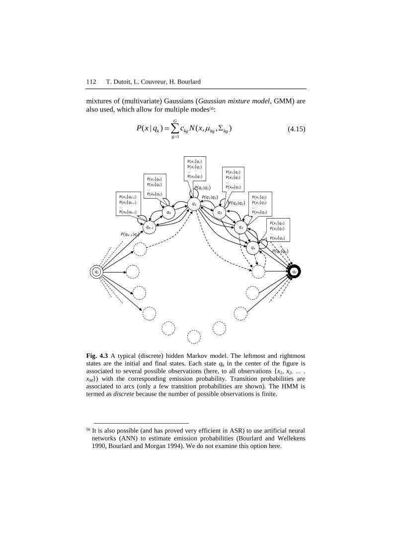
4.1.3 Hidden Markov models

Modifying a Markov model by allowing several states (if not all) to output

the same observations with state-dependent emission probabilities (Fig.

4.3), turns it into a hidden Markov model (HMM, Rabiner 1989). In such a

model, the sequence of states cannot be univocally determined from the

sequence of observations (such a SFSA is called ambiguous). The HMM is

thus called “hidden” because there is an underlying stochastic process (i.e.,

the sequence of states) that is not observable, but affects the sequence of

observations.

While Fig. 4.3 shows a discrete HMM, in which the number of possible

observations is finite, continuous HMMs are also very much used, in

which the output space is a continuous variable (often even multivariate).

Emission probabilities are then estimated by assuming they follow a

particular functional distribution: P(xm|qk) is computed analytically (it can

no longer be obtained by counting). In order to keep the number of HMM

parameters as low as possible, this distribution often takes the classical

form of a (multivariate, d-dimensional) Gaussian55:

1

1/ 2/ 2

( | ) ( , , )

1 1exp ( ) ( )

2(2 )

k k k

T

k k kd

k

P x q N x

x x

(4.14)

where μk and k respectively denote the mean vector and the covariance

matrix associated with state qk. When this model is not accurate enough,

55 Gaussian PDFs have many practical advantages: they are entirely defined by

their first two moments and are linear once derivated.


mixtures of (multivariate) Gaussians (Gaussian mixture model, GMM) are

also used, which allow for multiple modes56:

1

( | ) ( , , )G

k kg kg kg

g

P x q c N x

(4.15)

q1

q2

qK-1

P(x1|q4)

P(x2|q4)

…

P(xM|q4)

P(x1|qK-1)

P(x2|qK-1)

…

P(xN|qK-1)

P(x1|qK)

P(x2|qK)

…

P(xM|qK)

P(x1|q1)

P(x2|q1)

…

P(xM|q1) P(x1|q2)

P(x2|q2)

…

P(xM|q2)

P(x1|q3)

P(x2|q3)

…

P(xM|q3) qK

q3

q4

qI qF

P(q1|q2) P(q2|q2)

P(q1|q1)

P(qK-1|qI)

P(qF|q3)

Fig. 4.3 A typical (discrete) hidden Markov model. The leftmost and rightmost

states are the initial and final states. Each state qk in the center of the figure is

associated to several possible observations (here, to all observations {x1, x2, … ,

xM}) with the corresponding emission probability. Transition probabilities are

associated to arcs (only a few transition probabilities are shown). The HMM is

termed as discrete because the number of possible observations is finite.

56 It is also possible (and has proved very efficient in ASR) to use artificial neural

networks (ANN) to estimate emission probabilities (Bourlard and Wellekens

1990, Bourlard and Morgan 1994). We do not examine this option here.


where G is the total number of Gaussian densities and ckg are the mixture

gain coefficients (thus representing the prior probabilities of Gaussian

mixture components). These gains must verify the constraint:

1

1 1,...,G

kg

g

c k K

(4.16)

Assuming the total number of states K is fixed, the set of parameters of

the model comprises all the Gaussian means and variances, gains, and

transition probabilities.

Two approaches can be used for estimating ( | , )P X M .

In the full likelihood approach, this probability is computed as a sum on

all possible paths of length N. The probability of each path is itself

computed as in (4.7):

2

( | , ) (1) | (1) | (1) .

( ) | ( 1) ( ) | ( ) | ( )

j I j

paths j

N

j j j F j

n

P X M P q q P x q

P q n q n P x n q n P q q N

(4.17)

where qj(n) stands for the state in {q1, q2, … , qK} which is associated with

x(n) in path j. In practice, estimating the likelihood according to (4.17)

involves a very large number of computations, namely O(NKN), which can

be avoided by the so-called forward recurrence formula with a lower

complexity, namely O(K2N). This formula is based on the recursive

estimation of an intermediate variable n(l):

( ) (1), (2),..., ( ), ( )n ll P x x x n q n q (4.18)

n(l) stands for the probability that a partial sequence [x(1), x(2), . . . , x(n)]

is produced by the model in such a way that x(n) is produced by state ql. It

can be obtained by using (Fig. 4.4):

1

1

1

1

1

( ) ( (1) | ) | ( 1,..., )

2,..., ( 1,..., )

( ) ( ( ) | ) ( ) |

( | , ) ( ) ( ) |

l l I

K

n l n l k

k

K

N N F k

k

l P x q P q q l K

for n N and l K

l P x n q k P q q

P X M F k P q q

(4.19)


In the Viterbi approximation approach, the estimation of the data

likelihood is restricted to the most probable path of length N generating the

sequence X:

1

2

( | , ) max (1) | ) ( | (1) .

( ) | ( 1) | ( ) | ( )

j jpaths j

N

j j n j F j

n

P X M P q I P x q

P q n q n P x q n P q q N

(4.20

)

and the sums in (4.19) are replaced by the max operator. Notice it is also

easy to memorize the most probable path given some input sequence by

using (4.19) and additionally keeping in memory, for each n= (1,…,N) and

for each l=(1,…,K), the value of k producing the highest term of n+1(l) in

(4.19). Starting from the final state (i.e., the one leading to the highest term

for N+1(F)), it is then easy to trace back the best path, thereby associating

one "best" state to each feature vector.

q1

q2

q3

qK

q1 n(l)

n-1(1)

n-1(2)

n-1(3)

n-1(K)

P(ql|qk)

P(xn|ql)

Fig. 4.4 Illustration of the sequence of operations required to compute the

intermediate variable n(l)

HMMs are intensively used in ASR acoustic models where every

sentence model Mi is represented as a HMM. Since such a representation is

not tractable due to the infinite number of possible sentences, sentence

HMMs are obtained by compositing sub-sentence HMMs such as word

HMMs, syllable HMMs or more generally phoneme HMMs. Words,

syllables, or phonemes are then generally described using a specific HMM

topology (i.e. allowed state connectivity) known as left-to-right HMMs


(Fig. 4.5), as opposed to the general ergodic topology shown in Fig. 4.3.

Although sequential signals, such as speech, are nonstationary processes,

left-to-right HMMs assume that the sequence of observation vectors is a

piecewise stationary process. That is, a sequence X = [x(1), x(2), . . . , x(N)]

is modeled as a sequence of discrete stationary states with instantaneous

transitions between these states.

4.1.4 Training HMMs

HMM training is classically based on the Maximum Likelihood criterion:

the goal is to estimate the parameters of the model which maximize the

likelihood of a large number of training sequences Xj (j = 1,… , J). For

Gaussian HMMs (which we will examine here, as they are used in most

ASR systems), the set of parameters to estimate comprises all the Gaussian

means and variances, gains (if GMMs are used), and transition

probabilities.

q1

I

F q2

q3

Fig. 4.5 A left-to-right continuous HMM, shown here with (univariate) continuous

emission probabilities (which look like mixtures of Gaussians). In speech

recognition, this could be the model of a word or of a phoneme which is assumed

to be composed of three stationary parts.

Training algorithms

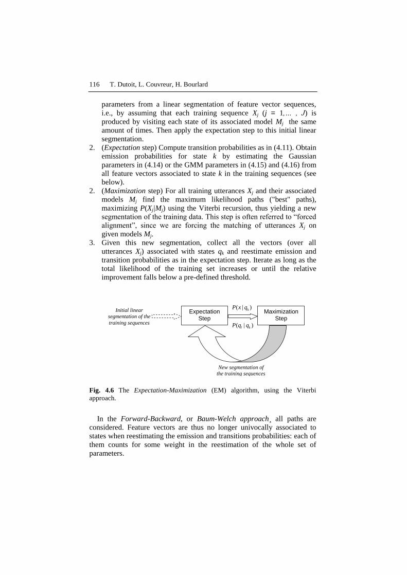
A solution to this problem is a particular case of the Expectation-

Maximization (EM) algorithm (Moon 1996). Again, two approaches are

possible.

In the Viterbi approach (Fig. 4.6), the following steps are taken:

1. Start from an initial set of parameters (0)

. With a left-to-right

topology, one way of obtaining such a set is by estimating the


parameters from a linear segmentation of feature vector sequences,

i.e., by assuming that each training sequence Xj (j = 1,… , J) is

produced by visiting each state of its associated model Mj the same

amount of times. Then apply the expectation step to this initial linear

segmentation.

2. (Expectation step) Compute transition probabilities as in (4.11). Obtain

emission probabilities for state k by estimating the Gaussian

parameters in (4.14) or the GMM parameters in (4.15) and (4.16) from

all feature vectors associated to state k in the training sequences (see

below).

2. (Maximization step) For all training utterances Xj and their associated

models Mj find the maximum likelihood paths ("best" paths),

maximizing P(Xj|Mj) using the Viterbi recursion, thus yielding a new

segmentation of the training data. This step is often referred to “forced

alignment”, since we are forcing the matching of utterances Xj on

given models Mj.

3. Given this new segmentation, collect all the vectors (over all

utterances Xj) associated with states qk and reestimate emission and

transition probabilities as in the expectation step. Iterate as long as the

total likelihood of the training set increases or until the relative

improvement falls below a pre-defined threshold.

Initial linear

segmentation of the

training sequences

Expectation Step

Maximization Step

( | )

( | )

k

l k

P x q

P q q

New segmentation of

the training sequences

Fig. 4.6 The Expectation-Maximization (EM) algorithm, using the Viterbi

approach.

In the Forward-Backward, or Baum-Welch approach¸ all paths are

considered. Feature vectors are thus no longer univocally associated to

states when reestimating the emission and transitions probabilities: each of

them counts for some weight in the reestimation of the whole set of

parameters.


The convergence of the iterative processes involved in both approaches

can be proved to converge to a local optimum (whose quality will depend

on the quality of the initialization).

Estimating emission probabilities

In the Viterbi approach, one needs to estimate the emission probabilities

of each state qk, given a number of feature vectors {x1k, x2k, …, xMk}

associated to it. The same problem is encountered in the Baum-Welch

approach, with feature vector partially associated to each state. We will

explore the Viterbi case here, as it is easier to follow57.

When a multivariate Gaussian distribution N(k,k) is assumed for some

state qk, the classical estimation formulas for the mean and covariance

matrix, given samples xik stored as column vectors, are:

1

1 M

k ik

i

xM

1

1( )( )

1

MT

k ik k ik k

i

x xM

(4.21)

It is easy to show that k is the maximum likelihood estimate of

k . The

ML estimator of k , though, is not exactly the one given by (4.21): the

ML estimator normalizes by M instead of (M-1). However it is shown to

be biased when the exact value of k is not known, while (4.21) is

unbiased.

When a multivariate GMM distribution is assumed for some state qk,

estimating its weights ckg, means kg and covariance matrices

kg for

g=1, …, G as defined in (4.15), cannot be done analytically. The EM

algorithm is used again for obtaining the maximum likelihood estimate of

the parameters, although in a more straightforward way than above (there

is not such a thing as transition probabilities in this problem). As before,

two approaches are possible: the Viterbi-EM approach, in which each

feature vectors is associated to one of the underlying Gaussians, and the

EM approach, in which each vector is associated to all Gaussians, with

some weight (for a tutorial on the EM algorithm, see Moon 1996, Bilmes

1998).

The Viterbi-EM and EM algorithms are very sensitive to the initial

values chosen for their parameters. In order to maximize their chances to

57 Details on the Baum-Welch algorithm can be found in (Bourlard, 2007).


converge to a global maximum of the likelihood of the training data, the k-

means algorithm is sometimes used for providing a first estimate of the

parameters. Starting from an initial set of G prototype vectors, this

algorithm iterates on the following steps:

1. For each feature vector xik (i=1, …, M), compute the squared Euclidian

distance from the kth prototype, and assign xik to its closest prototype.

2. Replace each prototype with the mean of the feature vectors assigned

to it in step 1.

Iterations are stopped when no further assignment changes occur.

4.2 MATLAB proof of concept: ASP_dictation_machine.m

Although speech is by essence a non-stationary signal, and therefore calls

for dynamic modeling, it is convenient to start this script by examining

static modeling and classification of signals, seen as a statistical pattern

recognition problem. We do this by using Gaussian multivariate models in

Section 4.2.1 and extend it to Gaussian Mixture Models (GMM) in Section

4.2.2. We then examine, in Section 4.2.3, the more general dynamic

modeling, using Hidden Markov Models (HMM) for isolated word

classification. We follow in Section 4.2.4 by adding a simple bigram-based

language model, implemented as a Markov model, to obtain a connected

word classification system. We end the Chapter in Section 4.2.5 by

implementing a word-based speech recognition system58, in which the

system does not know in advance how many words each utterance

contains.

4.2.1 Gaussian modeling and Bayesian classification of vowels

We will examine here how Gaussian multivariate models can be used for

the classification of signals.

A good example is that of the classification of sustained vowels, i.e., of

the classification of incoming acoustic feature vectors into the

corresponding phonemic classes. Acoustic feature vectors are generally

highly multi-dimensional (as we shall see later), but we will work in a 2D

space, so as to be able to plot our results.

58 Notice that we will not use the words classification and recognition

indifferently. Recognition is indeed more complex than classification, as it

involves the additional task of segmenting an input stream into segments for

further classification.


In this Chapter, we will work on a hypothetic language, whose phoneme

set is only composed of four vowels {/a/, /e/, /i/, /u/}, and whose lexicon

reduces to {"why" /uai/, "you" /iu/, "we" /ui/, "are" /ae/, "hear" /ie/, "here"

/ie/}. Every speech frame can then be represented as a 2-dimensional

vector of speech features in the form of pairs of formant values (the first

and the second spectral formants, F1 and F2; see Chapter 1, Section 1.1).

Our first task will be to classify vowels, by using Gaussian probability

density functions (PDF) for class models and Bayesian (MAP) decision.

Let us load a database of features extracted from the vowels and words of

this language59. Vowel samples are grouped in matrices of size N x 2,

where each of the N rows is a training example and each example is

characterized by a formant frequency pair [F1, F2]. Supposing that the

whole database covers adequately our imaginary language, it is easy to

compute the prior probability P(qk) of each class qk (qk in {/a/,/e/,/i/,/u/}).

The most common phoneme in our hypothetic language is /e/.

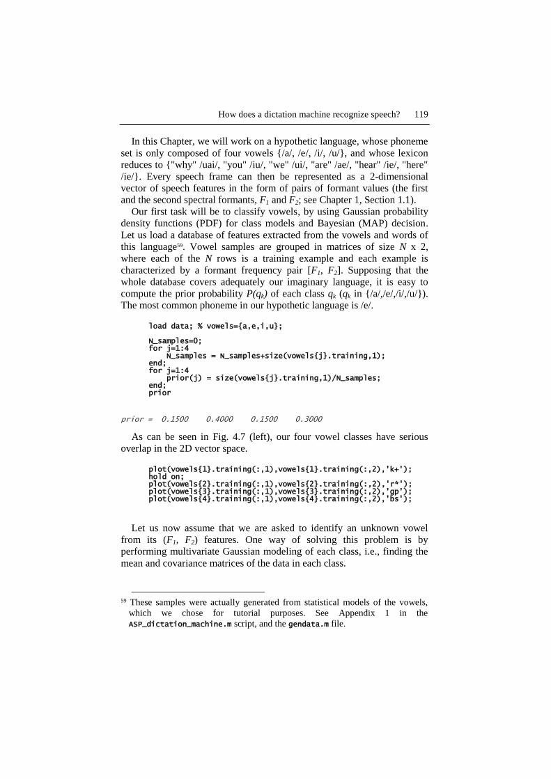
load data; % vowels={a,e,i,u}; N_samples=0; for j=1:4 N_samples = N_samples+size(vowels{j}.training,1); end; for j=1:4 prior(j) = size(vowels{j}.training,1)/N_samples; end; prior

prior = 0.1500 0.4000 0.1500 0.3000

As can be seen in Fig. 4.7 (left), our four vowel classes have serious

overlap in the 2D vector space.

plot(vowels{1}.training(:,1),vowels{1}.training(:,2),'k+'); hold on; plot(vowels{2}.training(:,1),vowels{2}.training(:,2),'r*'); plot(vowels{3}.training(:,1),vowels{3}.training(:,2),'gp'); plot(vowels{4}.training(:,1),vowels{4}.training(:,2),'bs');

Let us now assume that we are asked to identify an unknown vowel

from its (F1, F2) features. One way of solving this problem is by

performing multivariate Gaussian modeling of each class, i.e., finding the

mean and covariance matrices of the data in each class.

59 These samples were actually generated from statistical models of the vowels,

which we chose for tutorial purposes. See Appendix 1 in the

ASP_dictation_machine.m script, and the gendata.m file.


MATLAB function involved:

plot_2Dgauss_pdf(mu,sigma) plots the mean and standard deviation

ellipsis of the 2D Gaussian process that has mean mu and covariance

matrix sigma, in a 2D plot.

for j=1:4 mu{j}=mean(vowels{j}.training)'; sigma{j}=cov(vowels{j}.training); plot_gauss2D_pdf(mu{j},sigma{j}) end;

Fig. 4.7 Left: Samples of the four vowels {/a/, /e/, /i/, /u/} of our imaginary

language in the (F1,F2) plane, superimposed with the standard deviation ellipsis of

their 2D Gaussian model. Right: 2D Gaussian estimates of the PDF of these

vowels in the (F1,F2) plane.

Fig. 4.7 shows that /i/, for instance, has its mean F1 at 780 Hz and its

mean F2 at 1680 Hz 60. The covariance matrix for the /i/ class is almost

diagonal (the scatter plot for the class has its principal axes almost parallel

to the coordinate axes, which implies that F1 and F2 are almost

uncorrelated; see Appendix 1 of the ASP_dictation_machine.m file). Its

diagonal elements are thus close to the square of the length of the

halfmajor and halfminor axes of the standard deviation ellipsis: 76 Hz and

130 Hz, respectively.

60 These values are the ones fixed in our imaginary language; they do not

correspond to those of English vowels at all.


mu{3} sqrtm(sigma{3})

ans = 1.0e+003 * 0.7814 1.6827 ans = 75.3491 -4.4051 -4.4051 125.5608

Let us estimate the likelihood of a test feature vector given the Gaussian

model of class /e/, using the classical Gaussian PDF formula. The feature

vector is shown as a black dot in Fig. 4.7.

sample=[650 1903]; x = sample-mu{2}; likelihood = exp(-0.5* x* inv(sigma{2}) *x') / sqrt((2*pi)^2 … * det(sigma{2})) plot(sample(1),sample(2),'ko','linewidth',3)

likelihood = 7.1333e-007

The likelihood of this vector is higher in class /i/ than in any other class

(this is also intuitively obvious from the scatter plots shown previously), as

shown below.


gauss_pdf(x,mu,sigma) returns the likelihood of sample x (NxD)

with respect to a Gaussian process with mean mu (1xD) and covariance

sigma (DxD). When a set of samples is provided as input, a set of

likelihoods is returned.

for j=1:4 likelihood(j) = gauss_pdf(sample,mu{j},sigma{j}); end; likelihood

likelihood = 1.0e-005 * 0.0000 0.0713 0.1032 0.0000

Likelihood values are generally very small. Since we will use products

of them in the next paragraphs, we will systematically prefer their log-

likelihood estimates.

log(likelihood)

ans = -29.3766 -14.1533 -13.7837 -36.9803


Since not all phonemes have the same prior probability, Bayesian

(MAP) classification of our test sample is not equivalent to finding the

class with maximum likelihood. Posterior probabilities P(class|sample)

must be estimated by multiplying the likelihood of the sample by the prior

of each class, and dividing by the marginal likelihood of the sample

(obtained by summing its likelihood for all classes). Again, for

convenience, we compute the log of posterior probabilities. The result is

that our sample gets classified as /e/ ratter than as /i/, because the prior

probability of /e/ is much higher than that of /i/ in our imaginary language.

marginal=sum(likelihood); % is a constant log_posterior=log(likelihood)+log(prior)-log(marginal)

log_posterior = -18.0153 -1.8112 -2.4224 -24.9258

Notice that the marginal likelihood of the sample is not required for

classifying it, as it is a subtractive constant for all log posterior

probabilities. We will not compute it in the sequel.

Multiplying likelihoods by priors can be seen as a weighting which

accounts for the intrinsic frequency of occurence of each class. Plotting the

posterior probability of classes in the (F1, F2) plane gives a rough idea of

how classes are delimited (Fig. 4.7, right).


mesh_2Dgauss_pdf(mu,sigma,prior,gridx,gridy,ratioz) plots

the PDF of a 2D-Gaussian PDF in a 3D plot. mu (1x2) is the mean of the

density, sigma (2x2) is the covariance matrix of the density. prior is a

scalar used as a multiplicative factor on the value of the PSD. gridx and

gridy must be vectors of the type (x:y:z) ratioz is the (scalar) aspect

ratio on the Z axis.

hold on; for j=1:4 mesh_gauss2D_pdf(mu{j},sigma{j},prior(j),0:50:1500, ... 0:50:3000, 7e-9); hold on; end;

One can easily compare the performance of max likelihood vs. max

posterior classifiers on test data sets taken from our four vowels (and

having the same prior distribution as from the training set). The error rate

is smaller for Bayesian classification: 2.4% vs. 2.2%.



gauss_classify(x,mus,sigmas,priors) returns the class of the

point x (1xD) with respect to Gaussian classes, using Bayesian

classification. mus is a cell array of the (1xD) means, sigmas is a cell

array of the (DxD) covariance matrices. priors is a vector of Gaussian

priors. When a set of points (NxD) is provided as input, a set of classes is

returned. total=0; errors_likelihood=0; errors_bayesian=0; for i=1:4 n_test=size(vowels{i}.test,1); class_likelihood=gauss_classify(vowels{i}.test,mu,… sigma,[1 1 1 1]); errors_likelihood=errors_likelihood… +sum(class_likelihood'~=i); class_bayesian=gauss_classify(vowels{i}.test,mu,… sigma,prior); errors_bayesian=errors_bayesian… +sum(class_bayesian'~=i); total=total+n_test; end; likelihood_error_rate=errors_likelihood/total bayesian_error_rate=errors_bayesian/total

likelihood_error_rate = 0.0240 bayesian_error_rate = 0.0220

4.2.2 Gaussian Mixture Models (GMM)

In the previous section, we have seen that Bayesian classification is based

on the estimation of class PDFs. Up to now, we have modeled the PDF for

each class /a/, /e/, /i/, /u/ as a Gaussian multivariate (one per class). This

implicitly assumes that the feature vectors in each class have a (uni-modal)

normal distribution, as we used the mean and cov functions, which return

the estimates of the mean and covariance matrix of supposedly Gaussian

multivariate data samples. It turns out that the vowel data we used had

actually been sampled according to Gaussian distributions, so that this

hypothesis was satisfied.

Let us now try to classify the words of our imaginary language, using

the same kind of approach as above. We will use 100 samples of the six

words {"why" /uai/, "you" /iu/, "we" /ui/, "are" /ae/, "hear" /ie/, "here"

/ie/}61 in our imaginary language, for which each speech frame is again

61 Again, the phonetic transcriptions of these words are not those of English (while

they remain easy to remember for tutorial purposes).


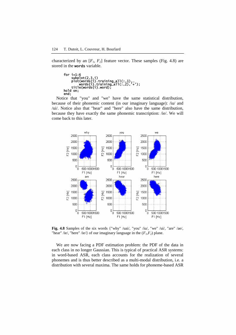
characterized by an [F1, F2] feature vector. These samples (Fig. 4.8) are

stored in the words variable.

for i=1:6 subplot(2,3,i) plot(words{i}.training_all(:,1),… words{i}.training_all(:,2),'+'); title(words{i}.word); hold on; end;

Notice that "you" and "we" have the same statistical distribution,

because of their phonemic content (in our imaginary language): /iu/ and

/ui/. Notice also that "hear" and "here" also have the same distribution,

because they have exactly the same phonemic transcription: /ie/. We will

come back to this later.

Fig. 4.8 Samples of the six words {"why" /uai/, "you" /iu/, "we" /ui/, "are" /ae/,

"hear" /ie/, "here" /ie/} of our imaginary language in the (F1,F2) plane.

We are now facing a PDF estimation problem: the PDF of the data in

each class in no longer Gaussian. This is typical of practical ASR systems:

in word-based ASR, each class accounts for the realization of several

phonemes and is thus better described as a multi-modal distribution, i.e. a

distribution with several maxima. The same holds for phoneme-based ASR


as well. As a matter of fact, speech is very much submitted to

coarticulation, which often results in several modes for the acoustic

realization of each phoneme, as a function of the phonetic context in which

it appears.

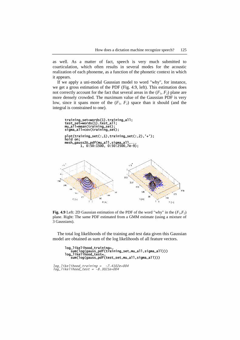
If we apply a uni-modal Gaussian model to word "why", for instance,

we get a gross estimation of the PDF (Fig. 4.9, left). This estimation does

not correctly account for the fact that several areas in the (F1, F2) plane are

more densely crowded. The maximum value of the Gaussian PDF is very

low, since it spans more of the (F1, F2) space than it should (and the

integral is constrained to one).

training_set=words{1}.training_all; test_set=words{1}.test_all; mu_all=mean(training_set); sigma_all=cov(training_set); plot(training_set(:,1),training_set(:,2),'+'); hold on; mesh_gauss2D_pdf(mu_all,sigma_all,... 1, 0:50:1500, 0:50:2500,7e-9);

Fig. 4.9 Left: 2D Gaussian estimation of the PDF of the word "why" in the (F1,F2)

plane. Right: The same PDF estimated from a GMM estimate (using a mixture of

3 Gaussians).

The total log likelihoods of the training and test data given this Gaussian

model are obtained as sum of the log likelihoods of all feature vectors.

log_likelihood_training=… sum(log(gauss_pdf(training_set,mu_all,sigma_all))) log_likelihood_test=… sum(log(gauss_pdf(test_set,mu_all,sigma_all)))

log_likelihood_training = -7.4102e+004 log_likelihood_test = -8.3021e+004


One way of estimating a multi-modal PDF is by clustering data, and

then estimate a uni-modal PDF in each cluster. An efficient way to do this

(using a limited number of clusters) is by using K-means clustering.

Starting with k prototype vectors or centroids, this algorithm first

associates each feature vector in the training set to its closest centroid. It

then replaces every centroid by the mean of all feature vectors that have

been associated to it. The algorithm iterates by re-associating each feature

vector to one of the newly found centroids, and so on until no further

change occurs.


[new_means,new_covs,new_priors,distortion]= ...

kmeans(data,n_iterations,n_clusters) , where data is the matrix of

observations (one observation per row) and n_clusters is the desired

number of clusters, returns the mean vectors, covariance matrices, and

priors of k-means clusters. distortion is an array of values (one per

iteration) of sum of squared distances between the data and the mean of

their cluster. The clusters are initialized with a heuristic that spreads them

randomly around mean(data). The algorithm iterates until convergence is

reached or the number of iterations exceeds n_iterations. Using

kmeans(data,n_iterations,means), where means is a cell array

containing initial mean vectors, makes it possible to initialize means.

plot_kmeans2D(data,means) plots the clusters associated with

means in data samples, using a Euclidian distance.

% Initializing prototypes "randomly" around the mean initial_means{1} = [0,1] * sqrtm(sigma_all) + mu_all; initial_means{2} = [0,0] * sqrtm(sigma_all) + mu_all; initial_means{3} = [1,2] * sqrtm(sigma_all) + mu_all; [k_means,k_covs,k_priors,totalDist]=kmeans(training_set,… 1000,initial_means); plot_kmeans2D(training_set, k_means);

The K-means algorithm converges monotonically, in 14 iterations, to a

(local) minimum of the global distortion defined as the sum of all distances

between feature vectors and their associated centroids (Fig. 4.10, left).

plot(totalDist,'.-'); xlabel('Iteration'); ylabel('Global LS criterion'); grid on;


Fig. 4.10 Applying the k-means algorithm (with k=3) to the sample feature vectors

for word "why". Left: Evolution of the total distortion; Right: Final clusters

The resulting sub-classes, though, do not strictly correspond to the

phonemes of "why" (Fig. 4.10, right). This is because the global criterion

that is minimized by the algorithm is purely geometric. It would actually

be very astonishing in these conditions to find the initial vowel sub-

classes. This is not a problem, as what we are trying to do is to estimate the

PDF of the data, not to classify it into "meaningful" sub-classes. Once

clusters have been created, it is easy to compute the corresponding

(supposedly uni-modal) Gaussian means and covariance matrices for each

cluster (this is actually done inside our kmeans function), and to plot the

sum of their PDFs, weighted by their priors. This produces an estimate of

the PDF of our speech unit (Fig. 4.9, right).


mesh_GMM2D_pdf(mus,sigmas,weights,gridx,gridy,ratioz) plots the PDF of a 2D Gaussian Mixture Model PDF in a 3D plot. mus is a

cell array of the (1x2) means, sigmas is a cell array of the (2x2) covariance

matrices. weights is a vector of Gaussian weights. gridx and gridy must

be vectors of the type (x:y:z) ratioz is the (scalar) aspect ratio on the Z

axis;

plot(training_set(:,1),training_set(:,2),'+'); hold on; mesh_GMM2D_pdf(k_means,k_covs,k_priors, ... 0:50:1500, 0:50:2500,2e-8); hold off;

The total log likelihoods of the training and test data are obtained as

above, except we now consider that each feature vector "belongs" to each

cluster with some weight equal to the prior probability of the cluster. Its


likelihood is thus computed as a weighted sum of likelihoods (one per

Gaussian).


GMM_pdf(x,mus,sigmas,weights) returns the likelihood of sample x

(1xD) with respect to a Gaussian Mixture Model. mus is a cell array of the

(1xD) means, sigmas is a cell array of the (DxD) covariance matrices.

(1xD) weight is a vector of Gaussian weights. When a set of samples

(NxD) is provided as input, a set of likelihoods is returned.

log_likelihood_training=… sum(log(GMM_pdf(training_set,k_means,k_covs,k_priors))) log_likelihood_test=… sum(log(GMM_pdf(test_set,k_means, k_covs, k_priors)))


The K-means approach used above is not optimal, in the sense that it is

based on a purely geometric convergence criterion. The central algorithm

for training GMMs is based on the EM (Expectation-Maximization)

algorithm. As opposed to K-means, EM truly maximizes the likelihood of

the data given the GMM parameters (means, covariance matrices, and

weights). Starting with k initial uni-modal Gaussians (one for each sub-

class), it first estimates, for each feature vector, the probability of each

sub-class given that vector. This is the Estimation step, which is based on

soft classification: each feature vector belongs to all sub-classes, with

some weights. In the Maximization step, the mean and covariance of each

sub-class is updated, using all feature vectors and taking those weights into

account. The algorithm iterates on the E and M steps, until the total

likelihood increase for the training data falls under some threshold.

The final estimate obtained by EM, however, only corresponds to a

local maximum of the total likelihood of the data, whose value may be

very sensitive to the initial uni-modal Gaussian estimates provided as

input. A frequently used value for these initial estimates is precisely the

one provided by the K-means algorithm.

Applied to the sample feature vectors of "why", the EM algorithm

converges monotonically, in 7 steps, from the K-means solution to a (local)

maximum of the total likelihood of the sample data (Fig. 4.11).



[new_means,new_sigmas,new_priors,total_loglike]= ...

GMM_train(data,n_iterations,n_gaussians), where data is the matrix

of observations (one observation per row) and n_gaussians is the desired

number of clusters, returns the mean vectors, covariance matrices, and

priors of GMM Gaussian components. total_loglike is an array of

values (one per iteration) of the total likelihood of the data given the GMM

model. GMMs are initialized with a heuristic that spreads them randomly

around mean(data). The algorithm iterates until convergence is reached or

the number of iterations exceeds n_iterations.

GMM_train(data,n_iterations,means,covs,priors) makes it possible

to initialize the means, covariance matrices, and priors of the GMM

components.

plot_GMM2D(data, means, covs) shows the standard deviation

ellipsis of the Gaussian components of a GMM defined by means and

covs, on a 2D plot, together with data samples.

[means,covs,priors,total_loglike]=GMM_train(training_set,… 100,k_means,k_covs,k_priors); plot(training_set(:,1),training_set(:,2),'+'); plot_GMM2D(training_set,means,covs); plot(total_loglike,'.-'); xlabel('Iteration'); ylabel('Global Log Likelihood'); grid on;

The total log likelihoods of the training and test data given this GMM

model are obtained as above. The increase compared to estimating the

GMM parameters from K-means clustering is small, but this is due to the

oversimplified PDF we are dealing with. GMMs are very much used in

speech recognition for acoustic modeling.

log_likelihood_training=… sum(log(GMM_pdf(training_set,means,covs,priors))) log_likelihood_test=… sum(log(GMM_pdf(test_set,means,covs,priors)))


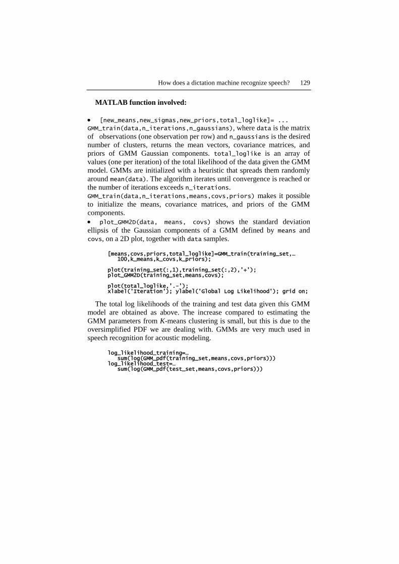
Fig. 4.11 Applying the EM algorithm (with 3 Gaussians) to the sample feature

vectors for word "why". Left: Evolution of the total log likelihood of the data;

Right: Standard deviation ellipses of the three Gaussian components. Notice we do

not set colors to feature vectors, as EM precisely does not strictly assign Gaussians

to feature vectors.


Now let us try to recognize sample words in {"why", "you", "we", "are",

"hear", "here"}. We now use the sequence of feature vectors from our

unknown signal (instead of a single vector as before), estimate the joint

likelihood of all vectors in this sequence given each class, and obtain the

posterior probabilities in the same way as above. If we assume that each

sample in our sequence is independent from the others (which is in

practice a rather bold claim, even for stationary signals; we will come back

to this in the next section when introducing dynamic models), then the

joint likelihood of the sequence is simply the product of the likelihoods of

each sample.

We first estimate a GMM for each word, using 3 Gaussians per word.62

The estimated GMMs are plotted in Fig. 4.12.

for i=1:6

[GMMs{i}.means,GMMs{i}.covs,GMMs{i}.priors,total_loglike]=... GMM_train(words{i}.training_all,100,3);

end;

for i=1:6 subplot(2,3,i)

62 When 2 Gaussians are enough, one of the three ends up having very small

weight.


plot(words{i}.training_all(:,1),… words{i}.training_all(:,2),'+'); title(words{i}.word); hold on; mesh_GMM2D_pdf(GMMs{i}.means,GMMs{i}.covs,GMMs{i}.priors, ... 0:50:1500, 0:50:2500,8e-9);

end;

Let us then try to recognize the first test sequence taken from "why"

(Fig. 4.13). Since we do not know the priors of words in our imaginary

language, we will set them all to 1/6. As expected, the maximum log

likelihood is encountered for word "why": our first test word is correctly

recognized.

word_priors=ones(1,6)*1/6; test_sequence=words{1}.test{1}; for i=1:6 log_likelihood(i) = sum(log(GMM_pdf(test_sequence,... GMMs{i}.means,GMMs{i}.covs,GMMs{i}.priors))); end; log_posterior=log_likelihood+log(word_priors) [maxlp,index]=max(log_posterior); recognized=words{index}.word

log_posterior = -617.4004 -682.0656 -691.2229 -765.6281 -902.7732 -883.7884 recognized = why

Fig. 4.12 GMMs estimated by the EM algorithm from the sample feature vectors

of our six words: "why", "you", "we", "are", "hear", "here"


Fig. 4.13 Sequence of feature vectors of the first sample of "why". The three

phonemes (each corresponding to a Gaussian in the GMM) are quite apparent.

Not all sequences are correctly classified, though. Sequence 2 is

recognized as a "we". test_sequence=words{1}.test{2}; for i=1:6 log_likelihood(i) = sum(log(GMM_pdf(test_sequence,... GMMs{i}.means,GMMs{i}.covs,GMMs{i}.priors))); end; log_posterior=log_likelihood+log(word_priors) [maxlp,index]=max(log_posterior); recognized=words{index}.word

log_posterior = 1.0e+003 * -0.6844 -0.6741 -0.6729 -0.9963 -1.1437 -1.1181 recognized = we

We may now compute the total word error rate on our test database.


GMM_classify(x,GMMs,priors) returns the class of sample x with

respect to GMM classes, using Bayesian classification. x {(NxD)} is a cell

array of test sequences. priors is a vector of class priors. The function

returns a vector of classes.

total=0; errors=0;


for i=1:6 n_test=length(words{i}.test); class=GMM_classify(words{i}.test,GMMs,word_priors); errors=errors+sum(class'~=i); class_error_rate(i)=sum(class'~=i)/n_test; total=total+n_test; subplot(2,3,i); hist(class,1:6); title(words{i}.word); set(gca,'xlim',[0 7]); end; overall_error_rate=errors/total class_error_rate

overall_error_rate = 0.3000 class_error_rate = 0.0800 0.4300 0.4400 0.0100 0.3900 0.4500

Obviously, our static approach to word classification is not a success.

Only 70% of the words are recognized. The rather high error rates we

obtain are not astonishing. Except for "why" and "are", which have fairly

specific distributions, "here" and "here" have identical PDFs, as well as

"you" and "we". These pairs of words are thus frequently mistaken for one

another (Fig. 4.14).

Fig. 4.14 Histograms of the outputs of the GMM-based word recognizer, for

samples of each of the six possible input words. The integer values on the x axes

refer to the index of the output word, in {"why", "you", "we", "are", "hear",

"here"}.


4.2.3 Hidden Markov Models (HMM)

In the previous Sections, we have seen how to create a model, either

Gaussian or GMM, for estimating the PDF of speech feature vectors, even

with complicated distribution shapes, and have applied it to the

classification of isolated words. The main drawback of such a static

classification, as it stands, is that it does not take time into account. For

instance, the posterior probability of a sequence of feature vectors does not

change when the sequence is time-reversed, as in words "you" /iu/ and

"we" /ui/. This is due to the fact that our Bayesian classifier implicitly

assumed that successive feature vectors are statistically independent.

In this Section we will model each word in our imaginary language

using a 2-state HMM (plus their initial and final states), except for "why",

which will be modeled as a 3-state HMM. One should not conclude that

word-based ASR systems set the number of internal HMM states for each

word to the number of phonemes they contain. The number of states is

usually higher than the number of phonemes, as phonemes are themselves

produced in several articulatory steps which may each require a specific

state. The reason for our choice is directly dictated by the fact that the test

data we are using throughout this script was randomly generated by

HMMs (see appendix 1 in the MATLAB script) in which each phoneme

was produced by one HMM state modeled as a multivariate Gaussian. As a

result, our test data virtually exhibits no coarticulation, and hence does not

require more than one state per phoneme.

We will make one more simplification here: that of having access to a

corpus of pre-segmented sentences, from which many examples of our 6

words have been extracted. This will make it possible to train our word

HMMs separately. In real ASR systems, segmentation (in words or

phonemes) is not known. Sentence HMMs are thus created by

concatenating word HMMs, and these sentence HMMs are trained. Words

(or phoneme) segmentation is then obtained as a by-product of this training

stage.

We start by loading our training data and creating initial values for the

left-right HMM of each word in our lexicon. Each state is modeled using a

Gaussian multivariate whose mean feature vector is set to a random value

close to the mean of all feature vectors in the word. The elements trans(i,j)

of the transition matrix give the probability of going from state qi to qj

(state 1 being the initial state). Transitions probabilities betweeen internal

(emiting) states are set to a constant value of 0.8 for staying in the same

state, and 0.2 for leaving to the next state.

% Initializing HMM parameters % "why" is a special case: it has 3 states


mu=mean(words{1}.training_all); sigma=cov(words{1}.training_all); HMMs{1}.means = {[],mu,mu,mu,[]}; HMMs{1}.covs = {[],sigma,sigma,sigma,[]}; HMMs{1}.trans = [ 0.0 1.0 0.0 0.0 0.0 0.0 0.8 0.2 0.0 0.0 0.0 0.0 0.8 0.2 0.0 0.0 0.0 0.0 0.8 0.2 0.0 0.0 0.0 0.0 1.0 ]; for i=2:6 mu=mean(words{i}.training_all); sigma=cov(words{i}.training_all); HMMs{i}.means = {[],mu,mu,[]}; HMMs{i}.covs = {[],sigma,sigma,[]}; HMMs{i}.trans = [0.0 1.0 0.0 0.0 0.0 0.8 0.2 0.0 0.0 0.0 0.8 0.2 0.0 0.0 0.0 1 ]; end

Let us train our HMM models using the Baum-Welch (or Forward-

Backward) algorithm, which is a particular implementation of the EM

algorithm we already used for training our GMMs in the previous Section.

This algorithm will adapt the parameters of our word HMMs so as to

maximize the likelihood of each training set given each HMM model.


new_hmm = HMM_train_FB(data,old_hmm,dmin,qmax)| returns the

Maximum Likelihood re-estimation of a Gaussian Hidden Markov Model

(i.e., a single, possibly multivariate, Gaussian probability density function

per state) based on the forward-backward algorithm (aka. Baum-Welch re-

estimation formulas). Note that most operations are performed in the log

domain for accuracy63. dmin and qmax are respectively the minimum log-

likelihood relative improvement and the maximum number of iterations

until convergence. for i=1:6 HMMs{i}=HMM_gauss_train(words{i}.training,HMMs{i},0.001,50); end;

The word "why" is now correctly modeled as a sequence of 3 states,

each with a Gaussian multivariate PDF, which matches those of the

underlying phonemes in the word: /uai/ (Fig. 4.15).

for i=2:4 subplot(1,3,i-1) plot(words{1}.training_all(:,1),… words{1}.training_all(:,2),'+'); title(['state ' num2str(i-1)]); % emiting states only

63 This function uses a homemade logsum.m function, which computes the log of a

sum of likelihoods from log-likelihoods, as mentioned in 4.1.1.


hold on; mesh_gauss2D_pdf(HMMs{1}.means{i},HMMs{1}.covs{i},1, ... 0:50:1500, 0:50:2500,1e-8); end;

Fig. 4.15 PDF of the three Gaussian HMM states obtained from samples of "why".

The transition probabilities between the states of "why" have been

updated by the Baum-Welch algorithm.

HMMs{1}.trans

ans = 0 1.0000 0 0 0 0 0.9970 0.0030 0 0 0 0 0.9951 0.0049 0 0 0 0 0.9387 0.0613 0 0 0 0 1.0000

As a result of this better modeling, the total likelihood of the data for

word "why" is higher than with our previous static GMM model. The

previous model can actually be seen as a single-state HMM, whose

emission probabilities are modeled by a GMM.

log_likelihood_training=0; for i=1:length(words{1}.training) training_sequence=words{1}.training{i}; log_likelihood_training=log_likelihood_training+... HMM_gauss_loglikelihood(training_sequence,HMMs{1}); end; log_likelihood_test=0; for i=1:length(words{1}.test) test_sequence=words{1}.test{i}; log_likelihood_test=log_likelihood_test+... HMM_gauss_loglikelihood(test_sequence,HMMs{1}); end;


log_likelihood_training log_likelihood_test


HMM-based isolated word classification can now be achieved by

finding the maximum of the posteriori probability of a sequence of feature

vectors given all 6 HMM models. The 2nd test sequence for "why" (which

was not correctly recognized using GMMs and a single state) now passes

our classification test.

word_priors=ones(1,6)*1/6; test_sequence=words{1}.test{2}; for i=1:6 log_posterior(i) = HMM_gauss_loglikelihood(... test_sequence, HMMs{i})+log(word_priors(i)); end log_posterior [tmp,index]=max(log_posterior); recognized=words{index}.word

log_posterior = 1.0e+003 * -0.6425 -1.0390 -0.6471 -1.0427 -1.1199 -1.1057 recognized = why

The HMM model does not strictly assign states to feature vectors: each

feature vector can be emitted by any state with a given probability. It is

possible, though, to estimate the best path through the HMM given the

data, by using the Viterbi algorithm (Fig. 4.16).


plot_HMM2D_timeseries(x,stateSeq) plots a two-dimensional

sequence x (one observation per row) as two separate figures, one per

dimension. It superimposes the corresponding state sequence stateSeq as

colored dots on the observations. x and stateSeq must have the same

length.

best_path=HMM_gauss_viterbi(test_sequence,HMMs{index}); plot_HMM2D_timeseries(test_sequence,best_path);

We may now compute the total word error rate again.


Fig. 4.16 Best path obtained by the Viterbi algorithm, from the sequence of

feature vectors of "why" in Fig. 4.13.


HMM_gauss_classify(x,HMMs,priors) returns the class of sample x

with respect to HMM classes, using Bayesian classification. HMM states

are modeled by a Gaussian multivariate. x (NxD) is a cell array of test

sequences. priors is a vector of class priors. The function returns a vector

of classes.

total=0; errors=0; for i=1:6 n_test=length(words{i}.test); class=HMM_gauss_classify(words{i}.test,HMMs,word_priors); errors=errors+sum(class'~=i); class_error_rate(i)=sum(class'~=i)/n_test; total=total+n_test; subplot(2,3,i); hist(class,1:6); title(words{i}.word); set(gca,'xlim',[0 7]); end; overall_error_rate=errors/total class_error_rate


overall_error_rate = 0.1600 class_error_rate = 0 0 0 0 0.4400 0.5200

Fig. 4.17 Histograms of the outputs of the HMM-based word classifier, for

samples of each of the six possible input words.

Notice the important improvement in the classification of "you" and

"we" (Fig. 4.17), which are now modeled as HMMs with distinctive

parameters. 84% of the (isolated) words are now recognized. The

remaining errors are due to the confusion between "here" and "hear".

4.2.4 N-grams

In the previous Section, we have used HMM models for the words of our

imaginary language, which led to a great improvement in isolated word

classification. It remains that "hear" and "here", having strictly identical

PDFs, cannot be adequately distinguished. This kind of ambiguity can only

be resolved when words are embedded in a sentence, by using constraints

imposed by the language on word sequences, i.e. by modeling the syntax

of the language.

We will now examine the more general problem of connected word

classification, in which words are embedded in sentences. This task

requires adding a language model on top of our isolated word classification

system. For convenience, we will assume that our imaginary language


imposes the same syntactic constraints as English. A sentence like "you are

hear" is therefore impossible and should force the recognition of "you are

here" wherever a doubt is possible. In this first step, we will also assume

that word segmentation is known (this could easily be achieved, for

instance, by asking the speaker to insert silences between words and

detecting silences based on energy levels).

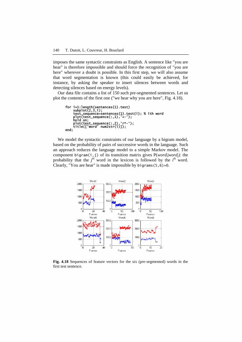
Our data file contains a list of 150 such pre-segmented sentences. Let us

plot the contents of the first one ("we hear why you are here", Fig. 4.18).

for i=1:length(sentences{1}.test) subplot(2,3,i); test_sequence=sentences{1}.test{i}; % ith word plot(test_sequence(:,1),'+-'); hold on; plot(test_sequence(:,2),'r*-'); title(['Word' num2str(i)]); end;

We model the syntactic constraints of our language by a bigram model,

based on the probability of pairs of successive words in the language. Such

an approach reduces the language model to a simple Markov model. The

component bigram(i,j) of its transition matrix gives P(wordi|wordj): the

probability that the jth word in the lexicon is followed by the i

th word.

Clearly, "You are hear" is made impossible by bigrams(5,6)=0.

Fig. 4.18 Sequences of feature vectors for the six (pre-segmented) words in the

first test sentence.


% states = I U {why,you,we,are,hear,here} U F % where I and F stand for the begining and the end of a sentence bigrams = ... [0 1/6 1/6 1/6 1/6 1/6 1/6 0 ; % P(word|I) 0 0 1/6 1/6 1/6 1/6 1/6 1/6; % P(word|"why") 0 1/5 0 0 1/5 1/5 1/5 1/5; % P(word|"you") 0 0 0 0 1/4 1/4 1/4 1/4; % P(word|"we") 0 0 1/4 1/4 0 0 1/4 1/4; % P(word|"are") 0 1/4 1/4 0 0 0 1/4 1/4; % P(word|"hear") 0 0 1/4 1/4 1/4 0 0 1/4; % P(word|"here") 0 0 0 0 0 0 0 1]; % P(word|F)

Let us now try to classify a sequence of words taken from the test set.

We start by computing the log likelihood of each unknown word given the

HMM model for each word in the lexicon. Each column of the log

likelihood matrix stands for a word in the sequence; each line stands for a

word in the lexicon {why,you,we,are,hear,here}.

n_words=length(sentences{1}.test); log_likelihoods=zeros(6,n_words); for j=1:n_words for k=1:6 % for each possible word HMM model unknown_word=sentences{1}.test{j}; log_likelihoods(j,k) = HMM_gauss_loglikelihood(... unknown_word,HMMs{k}); end; end; log_likelihoods

log_likelihoods = 1.0e+003 * -0.2754 -0.3909 -0.2707 -0.4219 -0.6079 -0.5973 -1.4351 -1.4067 -1.3986 -0.9186 -0.7952 -0.7977 -0.6511 -0.8062 -0.7147 -0.9689 -0.8049 -0.8024 -0.5203 -0.4208 -0.5043 -0.6925 -0.5306 -0.5284 -0.9230 -1.0715 -1.0504 -0.5506 -0.6912 -0.6935 -0.2510 -0.2772 -0.2400 -0.2851 -0.1952 -0.1953

With the approach we used in the previous Section, we would classify

this sentence as "we hear why you are hear" (by choosing the max

likelihood candidate for each word independently of its neighbors).

[tmp,indices]=max(log_likelihoods); for j=1:n_words recognized_sequence{j}=words{indices(j)}.word; end; recognized_sequence

recognized_sequence = 'we' 'hear' 'why' 'you' 'are' 'hear'


We implement our language model as a Markov model on top of our

word HMMs. The resulting model for the sequence to recognize is a

discrete HMM, in which there are as many internal states as the number of

words in the lexicon (six in our case). Each state can emit any of the

n_words input words (which we will label as '1', '2', ... 'n_words'), with

emission probabilities equal to the likelihoods computed above. Bigrams

are used as transition probabilities. Finding the best sequence of words

from the lexicon given the sequence of observations [1, 2, ..., n_words] is

obtained by looking for the best path in this model, using the Viterbi

algorithm again.

As shown below, we now correctly classify our test sequence as "we

hear why you are here".


[state,likelihood] = HMM_viterbi(transition,emission) performs the Viterbi search (log version) of the best state sequence for a

discrete Hidden Markov Model.

transition: (K+2)x(K+2) matrix of transition probabilities,

first and last rows correspond to initial and

final (non-emitting) states.

emission: NxK matrix of state-conditional emission

probabilities corresponding to a given sequence

of observations of length N.

state: (Nx1) vector of state-related indexes of best sequence.

likelihood: best sequence likelihood.

best_path=HMM_viterbi(log(bigrams),log_likelihoods); for j=1:n_words recognized_sequence{j}=words{best_path(j)}.word; end; recognized_sequence

recognized_sequence = 'we' 'hear' 'why' 'you' 'are' 'here'

We may finally compute the word error rate on our complete test data.

n_sentences=length(sentences); total=0; errors=0; class_error_rate=zeros(1,6); class=cell(6); % empty cells for i=1:n_sentences n_words=length(sentences{i}.test); log_likelihoods=zeros(6,n_words);


for j=1:n_words unknown_word=sentences{i}.test{j}; for k=1:6 % for each possible word HMM model log_likelihoods(j,k) = HMM_gauss_loglikelihood(... unknown_word,HMMs{k}); end; end; best_path=HMM_viterbi(log(bigrams),log_likelihoods); for j=1:n_words recognized_word=best_path(j); actual_word=sentences{i}.wordindex{j}; class{actual_word}= [class{actual_word}, … recognized_word]; if (recognized_word~=actual_word) errors=errors+1; class_error_rate(actual_word)=… class_error_rate(actual_word)+1; end; end; total=total+n_words; end; overall_error_rate=errors/total class_error_rate

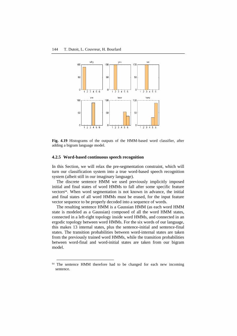
overall_error_rate = 0.1079 class_error_rate = 0 0 0 0 37 31

We now have an efficient connected word classification system for our

imaginary language. The final recognition rate is now 89.2%. Errors are

still mainly due to "here" being confused with "hear" (Fig. 4.19). As a

matter of fact, our bigram model is not constrictive enough. It still allows

non admissible sentences, such as in sentence #3: "why are you hear".

Bigrams cannot solve all "hear" vs. "here" ambiguities, because of the

weaknesses of this poor language model. Trigrams could do a much better

job ("are you hear", for instance, will be forbidden by a trigram language

model), at the expense of additional complexity.


Fig. 4.19 Histograms of the outputs of the HMM-based word classifier, after

adding a bigram language model.

4.2.5 Word-based continuous speech recognition

In this Section, we will relax the pre-segmentation constraint, which will

turn our classification system into a true word-based speech recognition

system (albeit still in our imaginary language).

The discrete sentence HMM we used previously implicitly imposed

initial and final states of word HMMs to fall after some specific feature

vectors64. When word segmentation is not known in advance, the initial

and final states of all word HMMs must be erased, for the input feature

vector sequence to be properly decoded into a sequence of words.

The resulting sentence HMM is a Gaussian HMM (as each word HMM

state is modeled as a Gaussian) composed of all the word HMM states,

connected in a left-right topology inside word HMMs, and connected in an

ergodic topology between word HMMs. For the six words of our language,

this makes 13 internal states, plus the sentence-initial and sentence-final

states. The transition probabilities between word-internal states are taken

from the previously trained word HMMs, while the transition probabilities

between word-final and word-initial states are taken from our bigram

model.

64 The sentence HMM therefore had to be changed for each new incoming

sentence.


sentence_HMM.trans=zeros(15,15); % word-initial states, including sentence-final state; word_i=[2 5 7 9 11 13 15]; word_f=[4 6 8 10 12 14]; % word-final states; % P(word in sentence-initial position) sentence_HMM.trans(1,word_i)=bigrams(1,2:8); % copying trans. prob. for the 3 internal states of "why" sentence_HMM.trans(2:4,2:4)=HMMs{1}.trans(2:4,2:4); % distributing P(new word|state3,"why") to the first states of % other word models, weighted by bigram probabilities. sentence_HMM.trans(4,word_i)=... HMMs{1}.trans(4,5)*bigrams(2,2:8); % same thing for the 2-state words for i=2:6 sentence_HMM.trans(word_i(i):word_f(i),word_i(i):word_f(i))=... HMMs{i}.trans(2:3,2:3); sentence_HMM.trans(word_f(i),word_i)=... HMMs{i}.trans(3,4)*bigrams(i+1,2:8); end;

The emission probabilities of our sentence HMM are taken from the

word-internal HMM states.

k=2; sentence_HMM.means{1}=[]; % sentence-initial state for i=1:6 for j=2:length(HMMs{i}.means)-1 sentence_HMM.means{k}=HMMs{i}.means{j}; sentence_HMM.covs{k}=HMMs{i}.covs{j}; k=k+1; end; end; sentence_HMM.means{k}=[]; % sentence-final state

We search for the best path in our sentence HMM65 given the sequence

of feature vectors of our test sequence, with the Viterbi algorithm, and plot

the resulting sequence of states (Fig. 4.20).


[states,log_likelihood] = HMM_gauss_viterbi(x,HMM) returns

the best state sequence and the associated log likelihood of the sequence of

feature vectors x (one observation per row) with respect to a Markov

model HMM defined by: HMM.means HMM.covs HMM.trans

65 The new sentence model is no longer sentence-dependent: the same HMM can

be used to decode any incoming sequence of feature vectors into a sequence of

words.


This function implements the forward recursion to estimate the likelihood

on the best path.

n_words=length(sentences{1}.test); complete_sentence=[]; for i=1:n_words complete_sentence=[complete_sentence ; ... sentences{1}.test{i}]; end; best_path=HMM_gauss_viterbi(complete_sentence,sentence_HMM); plot_HMM2D_timeseries(complete_sentence,best_path); state_sequence=best_path(diff([ 0 best_path])~=0)+1; word_indices=state_sequence(ismember(state_sequence,word_i)); [tf,index]=ismember(word_indices,word_i); recognized_sentence={}; for j=1:length(index) recognized_sentence{j}=words{index(j)}.word; end; recognized_sentence

recognized_sentence = 'we' 'hear' 'why' 'you' 'are' 'here'

We may finally compute again the word error rate on our complete test

data (this is done in the accompanying MATLAB script). The final error

rate of our word-based continuous speech recognizer is about 86.8%. This

is only 2.4% less than when using pre-segmented words, which shows the

efficiency of our sentence HMM model for both segmenting and

classifying words. In practice, non segmented data is used for both training

and testing, which could still slightly increase the word error rate.

Fig. 4.20 Best path obtained by the Viterbi algorithm, from the sequence of

feature vectors of the first test sentence.


4.3 Going further

Dictation machines still differ from this proof-of-concept in several

ways. Mel Frequency Cepstral Coefficients (MFCCs) are used in place of

our (F1, F2) formants for the acoustic model. Their first and second time-

derivatives are added as features, as a simple way of accounting for the

correlation between feature vectors within HMM states. Moreover, given

the number of possible words in natural languages (several tens of

thousands), ASR systems involve one additional layer in the statistical

description of sentences: that of phonemes. The word HMMs we have

trained above are replaced by phoneme HMMs. Word HMMs are

themselves composed of phoneme HMMs (in the same way as we have

built our sentence HMM from word HMMs), and additional pruning

mechanisms are used in the decoder to constrain the search for the best

sequence of words from the input feature vector sequence.

Several MATLAB-based HMM toolboxes are publicly available, such

as Kevin Murphy's (Murphy 2005), Steinar Thorvaldsen's (Thorvaldsen

2005, applied to biology), or Olivier Cappé's (Cappé 2001). MATLAB

also provides its own HMM toolbox under the Statistics Toolbox. The

most famous HMM toolbox, originally developed for large vocabulary

speech recognition, is the HTK toolkit developed at Cambridge University

(in ANSI C; Young et al. 2006).

4.4 Conclusion

In this Chapter, we have seen how GMMs are used for the classification of

(supposedly stationary) signals, and how HMMs provide a means of

modeling non-stationary signals as sequences of stationary states. We have

also implemented a simple bigram model, whose coupling with our word

HMMs has resulted in a unique sentence HMM, able to perform

continuous speech recognition, i.e., to find how many words are present in

an incoming stream of feature vectors, and which words they are.

4.5 References

Bilmes JA (1998) A gentle tutorial of the EM algorithm and its

applications t parameter estimation for Gaussian mixture and hidden

Markov models. Technical Report 97-021, ICSI, Berkeley, CA, USA.


Bourlard (2007) Automatic speech and speaker recognition. In: Speech

and Language Engineering. M. Rajman, ed., EPFL Press, pp 267-335

Bourlard H, Morgan N (1994) Connectionist Speech Recognition – A

Hybrid Approach. Kluwer Academic Publishers, Dordrecht.

Bourlard H, Wellekens C (1990) Links between Markov models and

multilayer perceptrons. IEEE Trans on Pattern Analysis and Machine

Intelligence, 12(12)

Cappé O (2001) H2M : A set of MATLAB/OCTAVE functions for the

EM estimation of mixtures and hidden Markov models [on line]

Available: http://www.tsi.enst.fr/~cappe/h2m/h2m.html [3/06/07]

Duda RO, Hart PE, Stork DG (2000) Pattern Classification. Wiley-

Interscience

Gold B, Morgan N (2000) Speech and Audio Signal Processing,

Processing and Perception of Speech and Music. Wiley, Chichester.

Jelinek F (1991) Up from Trigrams! Proceedings of Eurospeech 91,

Genova, vol. 3, pp 1037–1040

Moon TK (1996) The Expectation-Maximization Algorithm. IEEE Signal

Processing Magazine, 13 (6), pp 47–60

Murphy K (2005) Hidden Markov Model (HMM) Toolbox for Matlab [on

line] Available:

http://www.cs.ubc.ca/~murphyk/Software/HMM/hmm.html [20/05/07]

Picone JW (1993) Signal Modeling Techniques in Speech Recognition.

Proceedings of the IEEE, 81 (2), pp 1214–1247

Polikar R (2006) Pattern Recognition. In: Wiley Encyclopedia of

Biomedical Engineering, Akay M, Ed., New York, NY: Wiley

Rabiner LR (1989) A Tutorial on Hidden Markov Models and Selected

Applications in Speech Recognition. Proceedings of the IEEE, 77 (2),

pp 257–286

Thorvaldsen S (2005) A tutorial on Markov models based on Mendel's

classical experiments. Journal of Bioinformatics and Computational

Biology, Vol. 3, No. 6, 1441-1460. [on line] Available:

http://www.math.uit.no/bi/hmm/ [3/06/07]

Young S, Evermann G, Gales M, Hain T, Kershaw D, Liu X, Moore G,

Odell J, Ollason D, Povey D, Valtchev V, Woodland P (2006) The

HTK book (for HTK Version 3.4) [on line] Available:

http://htk.eng.cam.ac.uk/prot-docs/htkbook.pdf [3/06/07]

https://www.ppur.org/livres/978-2-940222-04-9.html

http://users.rowan.edu/~polikar/RESEARCH/PUBLICATIONS/wiley06.pdf

http://www.wiley.com/WileyCDA/WileyTitle/productCd-047124967X.html



http://en.wikipedia.org/wiki/Lawrence_Rabiner

http://www.caip.rutgers.edu/~lrr/Reprints/tutorial%20on%20hmm%20and%20applications.pdf



http://en.wikipedia.org/wiki/IEEE

http://www.worldscinet.com/jbcb/03/0306/S021972000500165X.html

http://htk.eng.cam.ac.uk/prot-docs/htkbook.pdf

how does a dictation machine recognize speech?

Documents