Finance and Economics Discussion SeriesDivisions of Research & Statistics and Monetary Affairs

Federal Reserve Board, Washington, D.C.

How Effective is Monetary Policy at the Zero Lower Bound?Identification Through Industry Heterogeneity

Arsenios Skaperdas

2017-073

Please cite this paper as:Skaperdas, Arsenios (2017). “How Effective is Monetary Policy at the Zero LowerBound? Identification Through Industry Heterogeneity,” Finance and Economics Discus-sion Series 2017-073. Washington: Board of Governors of the Federal Reserve System,https://doi.org/10.17016/FEDS.2017.073.

NOTE: Staff working papers in the Finance and Economics Discussion Series (FEDS) are preliminarymaterials circulated to stimulate discussion and critical comment. The analysis and conclusions set forthare those of the authors and do not indicate concurrence by other members of the research staff or theBoard of Governors. References in publications to the Finance and Economics Discussion Series (other thanacknowledgement) should be cleared with the author(s) to protect the tentative character of these papers.

How Effective is Monetary Policy at the Zero Lower Bound?Identification Through Industry Heterogeneity

Arsenios Skaperdas†‡

July 3, 2017First Draft: December 11, 2014

Abstract

US monetary policy was constrained from 2008 to 2015 by the zero lower bound, dur-ing which the Federal Reserve would likely have lowered the federal funds rate further ifit were able to. This paper uses industry-level data to examine how growth was affected.Despite the zero bound constraint, industries historically more sensitive to interest rates,such as construction, performed relatively well in comparison to industries not typicallyaffected by monetary policy. Further evidence suggests that unconventional policy low-ered the effective stance of policy below zero.

JEL Classification: E32, E43, E47, E52

†Board of Governors of the Federal Reserve System. Email: arsenios.skaperdas@frb.gov.‡I am thankful for the guidance of my dissertation advisors, Michael Hutchison and Carl Walsh, and

the members of my committee, David Draper and Ken Kletzer. I am also grateful to Johanna Francis forcontinued feedback and encouragement at an early stage. Michael Bergman, Valentina Colombo, CarlosDobkin, Peter Dunne, Gabriel Fagan, Benjamin Garcia, Stefan Gerlach, Matija Lorenz, Jeffrey Huther,Fergal McCann, Laura Moretti, Gerard O’Reilly, Jonathan Robinson, Ajay Shenoy, Evan Smith, Eric T.Swanson, UCSC Macro, Central Bank of Ireland, Workshop on Empirical Monetary Economics, and FedBoard seminar participants provided helpful comments. Finally, I thank the Monetary Policy Division atthe Central Bank of Ireland for an excellent environment to work on revising the paper during April toSeptember 2015. The views expressed in this paper are solely my own and should not be interpreted asreflecting the views of the Board of Governors of the Federal Reserve System or of anyone else associatedwith the Federal Reserve System.

1

1 Introduction

The federal funds rate reached essentially zero in December 2008, at which point theFederal Reserve could no longer provide further monetary accommodation through itstraditional policy instrument. Following that time, the unemployment rate continued torise, while inflation fell below target. The Federal Reserve would thus likely have loweredthe federal funds rate further if it were able to.

In order to continue influencing economic activity, the Federal Reserve turned to non-traditional policies. Among these, Large-Scale Asset Purchase programs (LSAPs) involvedthe purchases of assets while those purchases could no longer affect short-term interestrates. Instead, these programs were meant to lower longer-term interest rates, and influ-ence important yields affecting corporate bond and household mortgage rates. However,these programs were motivated by theoretical channels not believed to be particularlystrong before the crisis (Woodford, 2012; Walsh, 2014).

This paper examines growth during this unforeseen period of low interest rates andunconventional monetary policy. Given the scale of the Great Recession, estimates ofprevious behavior of the Federal Reserve indicate that the federal funds rate would likelyhave been decreased to -5 percent (Rudebusch, 2009). This suggests that a large amountof monetary accommodation- which had been provided in previous recoveries- did notoccur, unless unconventional policy had significant affects. Accordingly, one would expectthe recovery from the Great Recession to be weaker than previous recoveries. In that case,it would also necessarily be true that industry growth rates would be negatively affected.

The contribution of this paper is thus to ask the following question: did industriestypically affected by monetary policy suffer during the recovery from the Great Reces-sion? It is commonly thought that some industries are much more interest rate sensitivethan others. Using monetary vector autoregressions, I confirm that industries involvedin longer-term projects, or that require large consumer loans, such as construction anddurable goods manufacturing, respond more strongly to interest rate shocks (Dedola andLippi, 2005). I validate the industry ranking through an alternative measure of monetaryshocks from Romer and Romer (2004). If unconventional policy had little effect, we shouldexpect to see that these industries, such as construction, performed poorly in comparisonto industries not thought to be typically affected by monetary policy.

In contrast, I find that interest rate sensitive industries performed just as well- if notmore so- than in previous US recoveries. As firms also grew about as well on average as inprevious recoveries, it must be the case that either unconventional policy had significant

2

real effects, or that some other shocks on net caused heterogeneous industry effects as anexpansionary monetary shock would have. However, I find no evidence for any other suchshocks, including plausible alternative explanations such as expansionary fiscal policy orindustry-specific productivity growth.

In order to further answer whether unconventional monetary policy had real effects,I present a new time series method for measuring monetary accommodation. Departingfrom previous literature (Krippner, 2013; Wu and Xia, 2014; Lombardi and Zhu, 2014;Christensen and Rudebusch, 2013), I develop an approach that infers an implied mone-tary stance directly from observed industry growth rates and standard variables used inmonetary vector autoregressions. I find that that the zero lower bound period is char-acterized by “below zero” properties, in that observed outcomes occurred as if furtherfederal funds rate decreases had taken place. This provides evidence that unconventionalmonetary policy was effective, and accounts for the observed positive relative growth ratesof interest rate sensitive industries.

Overall, the findings in this paper mirror other results in the literature (Swansonand Williams, 2014; Gilchrist et al., 2014) which suggest that the Federal Reserve hadleeway to influence the economy through unconventional policy. Given the positive relativegrowth rates of interest rate sensitive industries, and measured accommodative monetaryshocks following the incidence of the zero bound, I infer suggestive evidence that thecombination of zero interest rates and unconventional policy increased economic activityin a comparable fashion to previous US recoveries for the public firms examined.

The layout of the paper is as follows: Section 2 establishes how this paper relates tothe literature on the zero lower bound. Sections 3, 4, and 5 explain the data, methodology,and results of the growth rates of interest rate sensitive industries through time. Section 6discusses alternative explanations for the findings. Section 7 presents explores whether theresults are attributable to unconventional monetary policy. Finally, Section 8 concludes.

2 Related Literature

The identification strategies of this paper rely in part on industry heterogeneity of theeffects of monetary policy. A variety of strands of literature have shown heterogeneous ef-fects. Barth and Ramey (2002) find that heterogeneous industry effects can arise from dif-fering degrees of working capital usage through the cost channel, whereby firms’ marginalcosts are directly affected by changes in nominal interest rates (Ravenna and Walsh, 2006).Gertler and Gilchrist (1994) find that small manufacturing firms are more responsive to

3

monetary policy shocks than large firms, and find evidence that this is at least partlydue to the credit channel. Ehrmann and Fratzscher (2004) and Maio (2013) examine het-erogeneous stock market movements in response to monetary shocks. Finally, structuralVAR evidence for heterogeneous industry effects can be found in Dedola and Lippi (2005)and Peersman and Smets (2005). The approach in this paper builds on that of Dedolaand Lippi (2005) in the basic specification of a VAR to identify how sectors respond tointerest rate shocks.

This paper’s results are particularly relevant in light of macro research that has impliedthat the effective short-term interest rate following 2008 was negative. Krippner (2013)and Wu and Xia (2014) use term structure models to calculate “shadow rates” of thestance of monetary policy, by evaluating what nominal interest rate would normally createobserved yield curves. These papers attempt to measure the short-term interest rateimplied by financial markets. In contrast, Section 7 estimates the effective federal fundsrate as implied by real macroeconomic variables and industry growth rates.

Finally, this paper follows Claessens et al. (2011) and in the use of firm-level datato answer macro questions. Claessens et al. (2011) examine the diffusion of the GlobalFinancial Crisis on firms from a large sample of countries using differences-in-differencesfrom the start of the crisis to the trough. In contrast, this paper examines economicrecoveries, and uses previous recoveries to benchmark what we should quantitatively ex-pect for firm growth. For the sectoral (industry) interest rate sensitivity index, I drawinspiration from Rajan and Zingales (1998) in capturing time-invariant intrinsic sectorcharacteristics.

The analysis in this paper has begun from the premise that interest rate decreases havenon-negligible effects on output. If this is not the case, this paper’s results provide nomeaningful evidence that monetary policy is effective at the zero lower bound. However,evidence for nominal rigidities is unambiguous (Steinsson and Nakamura, 2014; Gorod-nichenko and Weber, 2014). I thus proceed under the presumption that these rigiditiesdo result in real effects.

3 Data

3.1 Data Sources

I use Compustat data for access to a firm-level database with relevant firm covariates.This database contains quarterly and yearly information on the universe of publicly listed

4

companies in the US. As such, all results are local to public firms. In the conclusion, Idiscuss how representative is this sample of firms as a whole.

For ranking industry interest rate sensitivity, I use the Compustat Quarterly NorthAmerica database and the 1970:Q1-2008:Q3 time period. This sample is chosen such thatit precedes the crisis period and the incidence of the recovery at the zero lower bound. Ithen use the resulting ranking to predict revenue growth using Compustat annual data.All US macro data is from FRED. Fiscal variables are taken from the Bureau of EconomicAnalysis.

3.2 Industry Time Series Construction

To my knowledge, no consistent time series of industry growth exists.1 I thus constructtime series using Compustat data.

The timing of firm entry and exit into the Compustat database is an endogenous out-come of many variables. Regulatory changes, investor sentiment, and other factors couldmake it more appealing for firms to go public or merge during certain time periods. Whenexamining revenues, this would erroneously make it appear during times of increased cor-porate entry that an industry had grown (in aggregates) or shrunk (in averages, assumingentering firms are small). In fact, mean industry revenues do not follow any clear growthtrend. I thus examine growth rates of revenues rather than aggregates or averages.2

I follow the micro employment literature (Davis et al., 1998) in specifying firm-levelgrowth rates as

gi,j,t−k,t = yi,t − yi,t−k

0.5[yi,t + yi,t−k] (1)

Where yi,t is the variable of interest of firm i, in industry j, in quarter t. This bounds themeasure to a [−2, 2] interval and approximates the effect of log differences. This growthrate measure accounts for firm entry and exit symmetrically, corrects for the effects ofoutliers, and helps control for mergers.

Finally, I use year-over-year growth rates to avoid deseasonalizing. This ignores firmsthat exist for less than four quarters, provides a less volatile metric of firm growth thanquarter over quarter measures, and allows for firms that only report revenues once a yearover parts of the sample. The growth rate in quarter t of industry j is thus constructedas the industry average of (1)

1The Bureau of Economic Analysis does collect industry value added, among other variables, but hasno industry data spanning a time period long enough for a VAR analysis due to reclassification.

2I cannot calculate industry value added, as the Compustat database has only sparse data on wagesand salaries.

5

gj,t = 1nj,t

nj,t∑i=1

git−4,t (2)

Where nj,t is the number of firms in industry j at time t with year-over-year revenuestatistics.

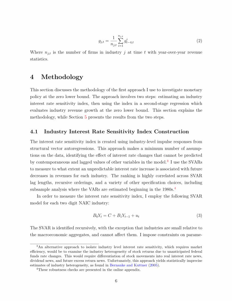
4 Methodology

This section discusses the methodology of the first approach I use to investigate monetarypolicy at the zero lower bound. The approach involves two steps: estimating an industryinterest rate sensitivity index, then using the index in a second-stage regression whichevaluates industry revenue growth at the zero lower bound. This section explains themethodology, while Section 5 presents the results from the two steps.

4.1 Industry Interest Rate Sensitivity Index Construction

The interest rate sensitivity index is created using industry-level impulse responses fromstructural vector autoregressions. This approach makes a minimum number of assump-tions on the data, identifying the effect of interest rate changes that cannot be predictedby contemporaneous and lagged values of other variables in the model.3 I use the SVARsto measure to what extent an unpredictable interest rate increase is associated with futuredecreases in revenues for each industry. The ranking is highly correlated across SVARlag lengths, recursive orderings, and a variety of other specification choices, includingsubsample analysis where the VARs are estimated beginning in the 1980s.4

In order to measure the interest rate sensitivity index, I employ the following SVARmodel for each two digit NAIC industry:

B0Yt = C +B1Yt−1 + ut (3)

The SVAR is identified recursively, with the exception that industries are small relative tothe macroeconomic aggregates, and cannot affect them. I impose constraints on parame-

3An alternative approach to isolate industry level interest rate sensitivity, which requires marketefficiency, would be to examine the industry heterogeneity of stock returns due to unanticipated federalfunds rate changes. This would require differentiation of stock movements into real interest rate news,dividend news, and future excess return news. Unfortunately, this approach yields statistically impreciseestimates of industry heterogeneity, as found in Bernanke and Kuttner (2005).

4These robustness checks are presented in the online appendix.

6

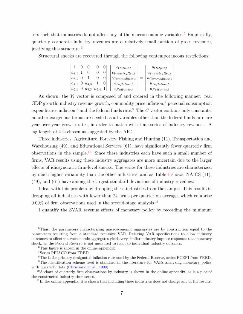
ters such that industries do not affect any of the macroeconomic variables.5 Empirically,quarterly corporate industry revenues are a relatively small portion of gross revenues,justifying this structure.6

Structural shocks are recovered through the following contemporaneous restrictions:

1 0 0 0 0a2,1 1 0 0 0a3,1 0 1 0 0a4,1 0 a4,3 1 0a5,1 0 a5,3 a5,4 1

εOutput,t

εIndustryRev,t

εCommodities,t

εInflation,t

εF edfunds,t

=

uOutput,t

uIndustryRev,t

uCommodities,t

uInflation,t

uF edfunds,t

As shown, the Yt vector is composed of and ordered in the following manner: real

GDP growth, industry revenue growth, commodity price inflation,7 personal consumptionexpenditures inflation,8 and the federal funds rate.9 The C vector contains only constants;no other exogenous terms are needed as all variables other than the federal funds rate areyear-over-year growth rates, in order to match with time series of industry revenues. Alag length of 4 is chosen as suggested by the AIC.

Three industries, Agriculture, Forestry, Fishing and Hunting (11), Transportation andWarehousing (49), and Educational Services (61), have significantly fewer quarterly firmobservations in the sample.10 Since these industries each have such a small number offirms, VAR results using these industry aggregates are more uncertain due to the largereffects of idiosyncratic firm-level shocks. The series for these industries are characterizedby much higher variability than the other industries, and as Table 1 shows, NAICS (11),(49), and (61) have among the largest standard deviations of industry revenues.

I deal with this problem by dropping these industries from the sample. This results indropping all industries with fewer than 24 firms per quarter on average, which comprise0.09% of firm observations used in the second-stage analysis.11

I quantify the SVAR revenue effects of monetary policy by recording the minimum

5Thus, the parameters characterizing macroeconomic aggregates are by construction equal to theparameters resulting from a standard recursive VAR. Relaxing VAR specifications to allow industryoutcomes to affect macroeconomic aggregates yields very similar industry impulse responses to a monetaryshock, as the Federal Reserve is not measured to react to individual industry oucomes.

6This figure is shown in the online appendix.7Series PPIACO from FRED.8The is the primary designated inflation rate used by the Federal Reserve, series PCEPI from FRED.9The identification scheme used is standard in the literature for VARs analyzing monetary policy

with quarterly data (Christiano et al., 1999).10A chart of quarterly firm observations by industry is shown in the online appendix, as is a plot of

the constructed industry time series.11In the online appendix, it is shown that including these industries does not change any of the results.

7

point estimate12 of the orthogonalized industry revenue response, over a four year hori-zon, to a positive one standard deviation interest rate shock from each SVAR in system(3). To ease interpretation of the index in predicting firm recovery, I standardize theorthogonalized impulse responses with respect to each other and multiply by −1. Insecond-stage regressions used to investigate the zero lower bound, this makes it such thata positive value on the index, denoted by φj, is associated with positive growth. Eachfirm i’s index sensitivity is based on its industry’s standardized orthogonalized impulseresponse. A one unit increase in the index thus signifies a one standard deviation increasein interest rate sensitivity.13

Formally, let χj = min16t=0

(∂gj,t

∂u5t

), where gj,t is the revenue growth rate at quarterly

horizon t for industry j, and u5t is a one standard deviation orthogonalized shock to thefederal funds rate. Then each firm in industry j has its interest sensitivity assigned to be

φj = −1 ·(χj − χj

σ

)(4)

where σ denotes the standard deviation of χj.

4.2 Second-Stage Analysis

I first use the industry ranking to trace out the time-varying evolution of the relativegrowth rates of industries identified as interest rate sensitive. This will reveal that interestrate sensitive industries have not suffered at the zero bound relative to historical norms.I then use the standardized sensitivity index to predict real revenue growth, as defined inequation (1), in the following more rigorous second-stage specification:

gi,j,t−k,t = ψ · (φjI2009,2012) + δφj + γt−k,tIt−k,t + βXi,j,t−k,t · It−k,t + εi,j,t−k,t (5)

Where gi,j,t−k,t is the revenue growth rate between years t−k and t of firm i, in industryj. It−k,t is an indicator for each of the three recoveries, while γt−k,t captures each recovery’strend growth. The coefficient ψ on the interaction term φjI2009,2012 captures the differencein real revenue growth for firms in sensitive industries relative to insensitive industries,

12Industries with positive responses to monetary shocks are thus set to zero before standardization.Alternative specifications of the index are presented in the online appendix and yield similar results.

13The literature on monetary policy has noted that the effects of monetary shocks are asymmetricdepending on the phase of the business cycle (Weise, 1999; Chen, 2007; Tenreyro and Thwaites, 2013).For example, a contractionary shock during an expansion may have different effects than a contractionaryshock during a recession. For the purposes of this paper, I examine the symmetric case, as is the case inthe majority of the VAR literature.

8

at the zero lower bound, in comparison to the previous two recoveries, captured by δ.In baseline specifications, I examine recoveries using the timing of 1991-1994, 2001-2004,and 2009-2012 for the recovery years, as these correspond to periods after which the Fedeased policy following a recession.14 The vector Xi,j,t−k,t consists of a number of controlvariables, to be explained, allowed to have different effects in each recovery.15 Equation5 is thus similar to running three separate OLS regressions over the periods 1991-1994.2001-2004, and 2009-2012, with the difference being that the correlation between industryrevenue growth and industry interest rate sensitivity is constrained to be the same over1991-1994 and 2001-2004 recoveries (δ), while I measure the difference in this correlationover the 2009-2012 ZLB period (ψ).

In all specifications, ψ captures the difference in revenues growth for firms in highlyinterest rate sensitive industries relative to firms in low sensitivity industries. If the zerobound has been a severely binding constraint on monetary policy, and hence aggregategrowth, it must be the case that industry growth rates have been negatively affected. Weshould then expect to see that ψ is significantly negative.

Table 11 presents summary statistics on relevant firm variables used in this paper. Itis of interest to note that the 2009-2012 recovery is not characterized by lower revenue oremployment growth than previous recoveries. In fact, the 2009-2012 period has greateremployment and revenue growth than the 2001-2004 recovery.

5 Empirical Results

5.1 SVAR Index Results

I first investigate the industry interest rate sensitivity classification. Figure 1 graphsthe orthogonalized industry impulse responses to an interest rate shock upon which thestandardized index is created.16 Table 2 presents the minimum response values to a one

14The year of each recovery start is set according to NBER dates. These most recent recoveries areexamined as they provide a closer comparison to the zero lower bound recovery rather than pre-GreatModeration. Examining other year choices for the recoveries give similar results.

15Note that the control variables are thus allowed to be time-varying. This is important because, forexample, industry GDP elasticity will have different effects depending on the strength of GDP growth,which varies across the three recoveries examined. Likewise, log firm employment at the start of eachrecovery may have different effects in 1991 than 2009, as firms on average are larger in 2009.

16In all figures, 90% standard error bands are calculated using a circular (moving block) bootstrap.Steps are as follows: an artificial time series is created, equal in length to the sample, using randomsamples of block length 4 drawn with replacement from a circle of the SVAR residuals, initiated with1971:Q1-1971:Q4 values. The SVAR models are estimated over the artificial time series, yielding distribu-

9

standard deviation shock, along with the standardized reciprocal explained previously.The ordering of industries aligns with common priors. Broadly speaking, industries clas-sified as more interest rate sensitive are capital intensive and produce goods of greaterdurability, as found in previous literature (Dedola and Lippi, 2005).17

According to the responses, Construction (23)18 and Mining, Quarrying, and Oil andGas Extraction (21)19 are the most sensitive sectors. These are industries that are highlyaffected by investment funding levels. The most responsive manufacturing sector, NAIC33, is composed mostly of durable goods (as in Erceg and Levin (2006)), which are in-tertemporally substitutable. Overall, the most sensitive sectors consist of firms that eitherundertake long-term projects sensitive to the cost of capital, or produce goods that requirelarge consumer loans.

Service industries including Health Care and Social Assistance (62), Professional, Sci-entific, and Technical Services (54), and Other Services (81), are less affected by interestshocks. These industries do not rely on inventory or production chains for revenues, mak-ing them less affected by the credit channel. Arts, Entertainment, and Recreation (71),though a service industry, may be more affected by decreases in disposable income.

The finding that the Retail Trade sectors (44 and 45) are not more affected may besurprising. However, it is important to note that uncertainty over the impulses responsesimplies that many of the industries with intermediate responses to interest rate shocks arenot statistically differentiable from each other. In addition, it is possible that exchangerate changes following interest rate changes mitigate the net effect on retail.

That utilities are somewhat affected by interest rates may be counterintuitive. Infact, utility companies have high debt loads,20 and many utility companies are subject toregulation which can cause decreases in their ability to adjust to interest rate changes.

It is important to mention that the ranking of industries by magnitude to an interestrate shock: construction, durable goods, non-durable goods, and the services sector, ismirrored by impulse response results from a VAR using these disaggregated components of

tions of impulse responses. This process is repeated 200 times. The standard error bands are calculatedusing the 5th and 95th empirical quantiles of the impulse responses at each horizon.

17These authors also find evidence that sensitive industries have higher degrees of working capitalusage and external financial dependence

18Evidence from the Bureau of Economic Analysis national accounts also shows that residential invest-ment is the most affected of all components of GDP by VAR interest rate shocks; as found by Bernankeand Gertler (1995).

19The oil and natural gas industries have similar rates of growth to other industries in NAIC 21, suchas coal mining, during the zero lower bound period.

20Of all industries, utility companies have the largest firm-year average of long term debt expense asa percent of total assets in sample.

10

GDP. Thus, the industry impulse responses using Compustat firms are similar to impulseresponses of aggregates from the national accounts.

The VAR impulse responses to an interest rate shock are shown in Figure 2. Althoughprices do rise initially in response to an interest rate shock, this increase is small andstatistically insignificant.21

5.2 Second-stage

CorrelationsIt is valuable to present the data in a graphical manner. Figure 3 charts coefficients

on interest rate sensitivity from three year industry-level growth rates regressed on yearindicators and year indicator-interest rate sensitivity index interactions. This charts theequivalent of the coefficient estimates on interest rate sensitivity (φj) in an OLS regressionover each three year window of revenue growth in the following regression.22

gj,t−k,t = α + βφj + εj,t−k,t (6)

The coefficients trace the time-varying association between interest rate sensitivity andrelative industry growth rates. As shown, the post-2009 period has a similar trajectoryto the 2001 recovery. This is a major finding of this paper. If the zero lower bound hasseverely constrained monetary policy, we should see that interest rate sensitive industrieshave been detrimentally affected. This is not the case.

Another interesting aspect of Figure 3 is that the pre-crisis years in the 2000s arecharacterized by large increases in revenues of interest rate sensitive industries. Ex-post, we now know that this time period was characterized by over-exuberant growthin industries sensitive to loosening credit standards. These are also the industries, suchas construction, which would be typically affected by monetary policy.23 Figure 3 isreassuring in the sense that it confirms the relevance of the interest rate sensitivity indexwith priors about how industries affected by monetary policy evolved before the crisis,though it does not prove that monetary policy was the cause of the buildup.

We would expect to see growth in interest rate sensitive industries in the post-1991

21The fact that prices initially rise as a result of a contractionary shock, the price puzzle, is a commonfinding in the literature. One theoretical reason proposed is the cost channel of monetary policy (Ravennaand Walsh, 2006). In a meta-analysis, Rusnak et al. (2013) find that the only consistent way to solve theprice puzzle is to implement sign restrictions which impose prices to decrease.

22Two year industry growth rates result in similar dynamics.23The finding that interest rate sensitive industries grew abnormally fast in the buildup to the crisis

is consistent with a vast literature examining the effects of the housing bubble (Mian and Sufi, 2009).

11

period. The fact that no such growth occurred is worrying given the substantial easingthat occurred during that time. However, the late 80s and early 90s were characterizedby a very high number of FDIC insured bank failures, as shown in Figures 4.24 Further-more, the savings and loans crisis contributed to a larger number of failures of financialintermediaries. If one takes the findings of this paper at face value, the Federal Reserve’sproactive actions in stabilizing the financial sector following the 2008 crisis were moreeffective at increasing the growth of interest rate sensitive industries than the easing thatoccurred in the 1990s. However, it is likely that other factors were also at play than mon-etary policy, which is not normally the predominant factor in business cycles, especiallyoutside of the zero bound. Thus, it may be the case that the post-2001 recovery pro-vides a better counterfactual for the zero lower bound period, with which the post-2009period still compares favorably. Regardless, the important aspect of Figure 3 is that thepost-crisis recovery, relative to historical norms, does not seem to be characterized by themonetary contraction implied by a severe liquidity trap.25

As a second exercise, I chart scatter plots of industry revenue growth rates and interestrate sensitivity in Figure 5. As mirrored in the preceding figure, the 1991-1994 recoveryis characterized by relatively little growth in interest rate sensitive industries. The post-2001 recovery is characterized by 5% growth for each standard deviation increase in indexsensitivity. Finally, the 2009 recovery is characterized by similar industry growth patternsto the post-2001 period. If the zero lower bound period resulted in roughly a 5% contrac-tionary monetary shock, as implied by Taylor rule type reaction functions (Rudebusch,2009), we would not expect industry revenue differentials due to interest rate sensitivityto be positive. There is no evidence here that interest rate sensitive industries have beendetrimentally affected by monetary policy during the zero lower bound period.

Econometric AnalysisTable 3 presents the basic test of this paper, estimating equation (5) at the firm-level.Firm-level data is useful, as it will allow firm-level controls. The coefficient on the in-dex interacted with 2009-2012 reveals that a one standard deviation increase in industrysensitivity is associated with positive increases in relative revenues over that period incomparison to previous recoveries, though this is statistically insignificant.26

24Of course, the Treasury and Federal Reserve also took actions that resulted in large bailouts followingthe 2008 financial crisis, while the FDIC was not as involved.

25Although Figure 3 appears to have a trend, this must be incidental, as it would imply that interestrate sensitive industries increasingly become a larger portion of the economy.

26The index coefficient itself equals zero, as it is a combination of the 2001-2004 recovery, which ischaracterized by negative growth, and 1991-1994, which is characterized by positive growth.

12

The fact that the interaction of the index and the 2009-2012 indicator is no less thanprevious recoveries is a major finding of this paper. Firms in industries typically sensitiveto monetary policy have not had diminished revenue growth in the current recovery,providing evidence that these industries have not been affected by the zero lower bound.Note that if spreads have moved differently relative to the federal funds rate since 2009,and transmission from the federal funds rate to other interest rates has been weaker, thisshould also result in a decreased coefficient for 2009-2012. We do not observe that this isthe case.

In order to rule out other factors that could bias the coefficients, I include controlvariables in columns (2) through (4). The control variables do not diminish the magnitudeof the coefficient ψ at the zero lower bound, meaning that the index is capturing variationseparate from traditional characteristics of firms affected by monetary policy. To showthat the results are not driven by business cycle variations, I include a sector level measureof GDP growth elasticity. Specifically, I regress revenue growth on annual GDP growthfor each sector using yearly data from 1985 to 2012. I then save each elasticity, andinteract it with GDP growth from each recovery in second-stage specification (3). Allresults are unchanged when controlling for sector-specific business cycle elasticities. Thisis reassuring, as it signifies that the VAR approach is capturing a shock which is orthogonalto industry-level GDP dependencies.

I include lagged log firm employment in the regression in column (3). Firm employ-ment at the start of each recovery could be correlated with firm revenue growth due tofinancing friction differences between small and large firms, as documented by Gertlerand Gilchrist (1994) in the manufacturing industry. In addition, important differences inemployment growth dynamics have been found across small and large firms, dependingon the aggregate unemployment rate (Moscarini and Postel-Vinay, 2012). The use offirm-level data provides the benefit of being able to adequately control for these factors.Reassuringly, the inclusion of firm employment does not change the relationship betweenthe index and firm revenue growth.

One possible confounder is that industry trends could be correlated with the interestrate sensitivity index, thus biasing the results. If firms ranked as sensitive have seculargrowth over the sample period, becoming a relatively larger share of output, this woulderroneously make it appear that sensitive firms grew more over the recovery periods dueto monetary policy. In order to test for this, I take quarterly firm averages of revenues ofeach NAIC sector from 1984-2008. I then calculate trend growth of revenues by regressingrevenues on a time trend. I use the predicted trend coefficient as a measure of secular

13

industry growth in the second-stage regressions. In all cases, this secular growth measuredoes not affect the results in any way, implying that secular trends are not driving theindex coefficient estimates.27

Although column (4) of Table 3 controls for secular industry trends over the sampleperiod, it is still possible that shorter growth trends could exist in industries sensitive tomonetary policy. If interest rate sensitive industries had relatively faster growth beforethe recoveries, and this differential continued, it would erroneously make it appear thatmonetary policy was causing the recovery. Table 4 estimates equation (5), using thetime periods preceding the recoveries (1988-1991, 1998-2001, and 2006-2009). The indexcoefficients are negative, meaning that there were industry pre-trends correlated withinterest rate sensitivity. However, the 2006-2009 coefficient estimate is not statisticallysignificant.

It is worrying that the index coefficients are significantly negative in Table 4, as itmeans that firms in interest rate sensitive industries suffered greater decreases in revenuesduring those recessions. It is often thought that recessions are followed by above-averagegrowth, returning economies to pre-recession trajectories of potential output. This wouldlikely be mirrored by above-average growth in industries that were hit hardest in therecession. If this is the case, we would expect the index coefficient to be of a strongermagnitude than in previous recoveries.28

In order to control for this potential mean reversion, I use three year lagged growthrates as control variables.29 Table 5 presents the results, showing that the index coefficientsfrom 2009-2012 are unchanged from Table 3, meaning that mean reversion cannot accountfor the growth in industries sensitive to monetary policy.30

The index φ is itself actually a generated variable, φ, whose uncertainty has not been

27This control variable is not interacted with the recovery indicators It−k,t, constraining it to have thesame value across recoveries. I do this since the purpose of the control variable is to show that growthrates during the recoveries are not driven by a single factor common across the time sample.

28Martin et al. (2014) examine HP filtered output before and after 149 recessions in advanced economiesfrom 1970, and find that, in fact, recessions are not followed by above average growth. Recessions arefollowed by decreased revisions of potential output. The authors state that it is likely researchers usingtwo-ended data find that the economy returns to potential, but with one-sided data, the true trend is notapparent.

29Specifically, I include the growth rates from 1988-1991, 1998-2001, and 2006-2009 interacted withthe recovery indicators in equation (5).

30Using the growth rates from 1988-1990, 1998-2000, and 2006-2008 as controls interacted with therecovery indicators yields the same results. Note that these estimates could be biased due to the corre-lation of firm fixed effects with the error term, though using previous years means that the firm fixedeffect is not mechanically correlated. Using lagged dependent variables as instruments is difficult in thiscontext given the small number of industry observations. In addition, controlling for firm employmenthelps to control for differential growth trends related to firm size.

14

taken into account thus far. Table 6 bootstraps over all possible indices to adjust forthis.31 The standard errors correcting for generated regressors are comparable to theindustry-clustered standard errors, though slightly larger on the index interactions. Thebootstrapped corrected standard errors do not meaningfully change the value of inferencefrom the results.

5.3 Romer and Romer’s Alternative Shock Measure

In this section, I provide external validation of the industry ordering using Romer andRomer (2004)’s alternative method to identify monetary shocks.32 The authors use in-ternal Fed forecasts to construct a series of intended federal funds rate changes that arepurged of information of future output and inflation. This leaves variation that shouldbe orthogonal to developments of these variables, allowing the series to be used as anexplanatory variable while being relatively free of endogeneity.

Following Coibion (2012), I cumulate R&R’s shock measures and use it in hybridVARs, analogous to (3), with the cumulative new shock measure in place of the federalfunds rate.33 I construct the index using the SVAR impulse responses in the same fashionas explained in Section 4.1. The resulting industry ordering using R&R has a correlationof 0.85 with the baseline SVAR index (Table 7). Thus, using the federal funds rate or theR&R shock measure results in a very similar industry ordering. Likewise, controlling forfiscal variables, and using non-financial output in the VARs with the R&R shocks resultsin a highly correlated measure.34 Table 8 reveals that second-stage estimates using theR&R shock series result in zero lower bound estimates that are quite similar to the resultsusing the federal funds rate, though the third column does have increased standard errors.

31Pagan (1984) has shown that equation (5) will yield inconsistent standard errors if uncertainty fromindex construction is not taken into account. I employ a bootstrapping technique to show that correctingfor generated regressors does not change the statistical significance of coefficients. For each sequence ofimpulse responses, 200 possible indices are created from each iteration of industry SVARs described inFootnote 16. An index is drawn with replacement from this distribution, then 19 industry clusters aredrawn with replacement for the second-stage, and Equation (5) is run. The standard deviations of thepoint estimates are then the bootstrapped standard errors of the coefficients. Industry-level data is usedfor this calculation so as to decrease computational burden.

32The shock series, updated and used from 1971:Q1-2007:Q4, can be obtained from Silvia Tenreyro’swebsite.

33The hybrid VAR methodology involves summing up the series of shocks up to time t for each t inthe sample. This creates a level series comparable to the federal funds rate for the VARs, except that itcontains only exogenous movements of the interest rate as identified by R&R. I use hybrid VARs sincethis helps to control for many factors that can cause ommitted variables relative to a univariate regressionwith volatile industry data.

34The specification of the SVARs for this index is expanded upon in Section 7.

15

6 Possible Alternative Explanations

6.1 Productivity Increases

In a recovery generated by monetary policy, we would expect revenues in industries pos-itively affected by monetary policy to have proportional increases in hours. That is, wewould expect sectors to have movements along their production functions, rather thanshifts in their production functions due to technological advances.

Recent literature (Fernald, 2014) has found diminished productivity growth leadingup to and through the Great Recession. Nonetheless, a formal test of productivity growthagainst the monetary industry index is necessary.

Table 9 estimates equation (5) with real revenues over employment growth, for ameasure of labor productivity, as the independent variable.35 In none of the the recoveriesis the index significant, meaning that firm labor productivity growth cannot account forthe growth of interest rate sensitive industries, including at the zero bound.

I additionally test for the interaction between multi-factor productivity growth andthe sensitivity index by using data from Rosenthal et al. (2014). The authors combineindustry-level output and intermediate inputs from the Bureau of Economic analysis withcapital and labor statistics from the BLS Productivity Program to calculate contributionsto aggregate growth in value-added by industry. The data is aggregated slightly differentlythan NAICs code. Specifically, the authors have a durable and non-durable categorization.I thus assign durable goods to be NAIC 33, and 31 and 32 to be non-durables, as the3-digit NAIC categorizations fall mostly along this line.36

Figure 6 presents scatter plots and an OLS regression of the sensitivity index andmulti-factor productivity growth from 2009-201237 by 2-digit NAIC industry. As shownin the figure, there is little relationship. Thus, productivity increases cannot account forthe positive coefficient on the index sensitivity index, and are not biasing the results. 38

35Bureau of Labor Statstics data reveals that correlations between employment and hours worked in1991,1994, 2009, and 2012 are all greater than 0.98. The correlations in 2001 and 2004 are 0.895 and 0.921respectively. Hence, the BLS data suggests that using employment as a proxy for hours from 2009-2012is acceptable.

36The mapping from Rosenthal et al. (2014)’s study to NAIC 31, 32, and 33, does not affect the results.For retail trade, I assign both NAIC groups (44 and 45) to the same value that the authors provide.

37These are the only years for which multi-factor productivity growth data is available, so I cannottest the relationship for 1991-1994 and 2001-2004.

38Including multi-factor productivity growth in Equation 1 leaves coefficient estimates in the regressionunchanged.

16

6.2 Fiscal Policy

One observationally equivalent explanation for the positive coefficient on interest ratesensitivity from 2009-2012 is that fiscal policy was able to counteract the effects of a con-tractionary monetary shock. Faced with the greatest financial crisis since the Great De-pression, Congress passed the American Recovery and Reinvestment Act of 2009 (ARRA)in February of that year. The economic stimulus package resulted in an estimated $831billion increase in spending between 2009 and 2019, including increases in unemploymentbenefits, and direct spending on infrastructure.

The literature has found that the net effect of ARRA was relatively small. In compar-ison to a panel of countries, Aizenman and Pasricha (2013) find that the US was ranked inthe bottom third in growth of public spending. Likewise, Aizenman and Pasricha (2010)find that after factoring in decreases in state and local government spending, consolidatedgovernment spending was insufficient to counteract decreases in private demand. Theseevaluations of ARRA are corroborated by Cogan et al. (2010). The authors estimate theoutput effects of government purchases using the Smets-Wouters model, and find maxi-mum effects of 0.3% of GDP in 2009:Q3. Following the end of the Great Recession, fiscalpolicy was unprecedentedly contractionary (Cashin et al., 2016).39

I thus control for fiscal policy by constructing an industry-level measure of the effectsof government spending in a similar to manner to the approach for measuring interest ratesensitivity. I run VARs for each industry while adding the growth rates of governmentspending40 and tax receipts as the first and second ordered variables in the VAR. TheVAR specification is described at greater length in Section 7. I quantify the resultingindustry responses to government spending by summing the cumulative response over a16 quarter horizon to an orthogonalized government spending shock.41 The cumulativeindustry responses are then standardized with respect to each other.

The resulting measure of industry sensitivity to fiscal policy is negatively correlatedwith the baseline interest rate sensitivity index (ρ = −0.37).42 This negative correlationis intuitive, as interest rate sensitive industries would also be sensitive to increases ininterest rates due to crowding out, as long as they are not disproportionately awardedgovernment funds. Mining, Quarrying, and Natural Gas, for example, was found to be

39Quarterly year-over-year growth rates of government consumption and investment spending werenegative from mid-2010 to mid-2014.

40The series used is government consumption and gross investment from the National Accounts.41Note that since government spending shocks can have both positive and negative industry revenue

effects due to crowding out, the cumulative sum of the revenue impulse response is a more adequatemeasure than the minimum used for constructing industry interest rate sensitivity

42The resulting fiscal policy sensitivity index is presented in the online appendix.

17

highly sensitive to interest rates. Similarly, a positive government spending shock resultsin a decrease in revenue for this industry.43

Including industries’ sensitivity to fiscal policy to the baseline regressions of this paperdoes not change the finding that the zero bound recovery is no different than previousrecoveries. Column (2) of Table 10 controls for industry sensitivity to fiscal policy. Thesecond-stage estimates of industry interest rate sensitivity during the zero bound, thoughdiminished, are not significantly different from other recoveries. Column (3), which in-cludes controls, yields similar results. Interestingly, the coefficient on fiscal policy sensi-tivity interacted with the zero bound period shows that those industries fared significantlyworse in revenue growth than during other times. This is consistent with unprecedentedfiscal contraction during the zero bound decreasing growth.

7 Identifying the Policy Stance

7.1 Methodology

Thus far, evidence on monetary policy effectiveness has been presented through an infer-ential approach comparing recoveries. In this section, I evaluate how much the results areattributable to unconventional policy, and provide time series rather than cross-sectionalevidence that the zero lower bound period was characterized by accommodative monetarypolicy.

I find evidence that unconventional policy succeeded in stimulating growth in excess ofwhat a federal funds rate of zero would suggest. I infer the implied policy stance based onthe estimated SVARs, growth rates of industry revenues, and macroeconomic aggregatesused throughout the paper. The method uses the Kalman filter to extract a measure ofthe interest rate shocks on a quarterly basis from the structural forms of the models in(3). For expositional purposes, consider a bivariate VAR(1) system in structural form

B0Yt = B1Yt−1 + ut (7)

Rewriting as explicit equations for the two variables while assuming a recursive ordering,and letting (i, j) denote the ith row and jth column of the preceding matrix,

xt = B1(1, 1)xt−1 +B1(1, 2)zt−1 + u1t (8)

zt = −B0(2, 1)xt +B1(2, 2)xt−1 +B1(2, 1)zt−1 + u2t

43These impulse responses are presented in the online appendix.

18

Notice that by construction, the structural shocks u1t and u2t are uncorrelated witheach other, and are assumed to be normal with sufficient lag length. This implies thatgiven data and parameters, (8) can be reformulated as a state-space model that can besolved using the Kalman filter out-of-sample. In brief, the Kalman filter minimizes onestep ahead prediction errors, optimally weighting the uncertainty of the measurementequation and the uncertainty of the state.

Assume VAR parameters have been solved for using a sample of observed values. Thenin state-space form the measurement equation is as follows:

xt = B0(1, 1)xt−1︸ ︷︷ ︸deterministic

+(B1)(1, 2)zt−1 + u1t (9)

while the state equation is defined as:

zt = −B0(2, 1)xt + (B1)(2, 2)xt−1︸ ︷︷ ︸deterministic

+B1(2, 1)zt−1 + u2t (10)

Using the observed series xt, the unobserved series zt can be solved for using Kalman filter,both in or out-of-sample, using the estimated VAR parameters in the B matrices. Out-of-sample, the Kalman filter is essentially decomposing the forecast errors of structuralforecasts of the SVAR equations into an interest rate component and other disturbances.

I make three main changes from the baseline SVARs used throughout the paper.44 Asshown in the industry impulse responses in Figure 1, the financial sector (NAIC 52) has astarkly different response to a monetary contraction than any other industry, with a largeinitial increase in revenues, followed by a subsequent decrease to negative growth. In theshort run, financial firms can benefit from increased interest rates, and hence larger spreadsbetween short and long-term rates, before the macroeconomic effects of monetary policydepress output. As a result of the strong response of the financial sector, VARs examiningthe post-1980 subsample often find indeterminate output responses to monetary shocks.45

I thus place non-financial corporate output into the SVARs in place of GDP growth,46

as the Kalman filter cannot accurately extract monetary shocks following the 1980s if animportant measurement equation capturing aggregate demand ceases being informative.

44The resulting industry interest sensitivity ranking is highly correlated (ρ > 0.8) regardless of thesechanges, as shown in Section 5.3.

45A second reason has been proposed in the monetary VAR literature for the weak response of outputto monetary shocks for post-1980 subsamples. Boivin and Giannoni (2006) find that by responding morestrongly to inflation, monetary policy has been more effective in counteracting shocks since the 1980s.Since interest rate movements are more systematic and endogenous than in earlier periods, VARs areunable to identify the effects of unsystematic interest rate shocks.

46This follows Lozej (2012).

19

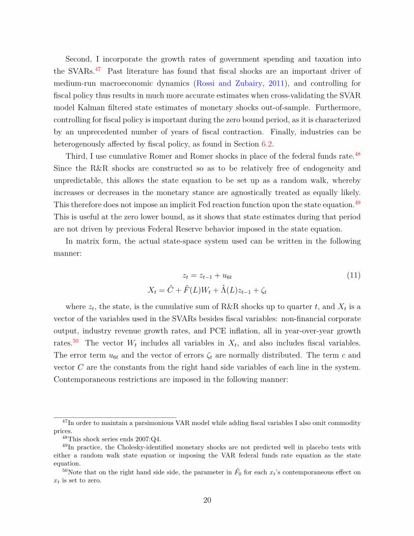
Second, I incorporate the growth rates of government spending and taxation intothe SVARs.47 Past literature has found that fiscal shocks are an important driver ofmedium-run macroeconomic dynamics (Rossi and Zubairy, 2011), and controlling forfiscal policy thus results in much more accurate estimates when cross-validating the SVARmodel Kalman filtered state estimates of monetary shocks out-of-sample. Furthermore,controlling for fiscal policy is important during the zero bound period, as it is characterizedby an unprecedented number of years of fiscal contraction. Finally, industries can beheterogenously affected by fiscal policy, as found in Section 6.2.

Third, I use cumulative Romer and Romer shocks in place of the federal funds rate.48

Since the R&R shocks are constructed so as to be relatively free of endogeneity andunpredictable, this allows the state equation to be set up as a random walk, wherebyincreases or decreases in the monetary stance are agnostically treated as equally likely.This therefore does not impose an implicit Fed reaction function upon the state equation.49

This is useful at the zero lower bound, as it shows that state estimates during that periodare not driven by previous Federal Reserve behavior imposed in the state equation.

In matrix form, the actual state-space system used can be written in the followingmanner:

zt = zt−1 + u6t (11)

Xt = C + F (L)Wt + Λ(L)zt−1 + ζt

where zt, the state, is the cumulative sum of R&R shocks up to quarter t, and Xt is avector of the variables used in the SVARs besides fiscal variables: non-financial corporateoutput, industry revenue growth rates, and PCE inflation, all in year-over-year growthrates.50 The vector Wt includes all variables in Xt, and also includes fiscal variables.The error term u6t and the vector of errors ζt are normally distributed. The term c andvector C are the constants from the right hand side variables of each line in the system.Contemporaneous restrictions are imposed in the following manner:

47In order to maintain a parsimonious VAR model while adding fiscal variables I also omit commodityprices.

48This shock series ends 2007:Q4.49In practice, the Cholesky-identified monetary shocks are not predicted well in placebo tests with

either a random walk state equation or imposing the VAR federal funds rate equation as the stateequation.

50Note that on the right hand side side, the parameter in F0 for each xt’s contemporaneous effect onxt is set to zero.

20

1 0 0 0 0 0a2,1 1 0 0 0 0a3,1 a3,2 1 0 0 0a4,1 a4,2 a4,3 1 0 0a5,1 a5,2 a5,3 0 1 00 0 a6,3 0 a6,5 1

εGovtCons,t

εT ax,t

εNF Coutput,t

εIndustryRev,t

εInflation,t

εR&Rshocks,t

=

uGovtCons,t

uT ax,t

uNF Coutput,t

uIndustryRev,t

uInflation,t

uR&Rshocks,t

The model is essentially Cholesky identified with fiscal variables ordered first, with

a few differences. As before, industry revenues are constrained to not affect any othervariables either contemporaneously or through lagged parameters. I also impose that theRomer and Romer shocks are not affected by fiscal policy contemporaenously or throughlagged parameters.51

The SVARs are run, yielding structural forms for the federal funds rate, macro vari-ables, and industry revenues.52 I then input the parameters and data from both the1971:Q1-2007:Q4 and post-2008 period into system (11), treating F (L)Wt as exogenousdisturbances to the measurement equations. Finally, I run the Kalman filter on thissystem, treating zt as the unobserved state.

It is important to mention an aspect of the estimated state series zt. This method doesnot explicitly capture a market “shadow” interest rate as other papers in the literaturehave done (Wu and Xia, 2014). The state series after 2008:Q3 is yielding an estimate ofcumulative Romer and Romer shocks that would imply the realizations of Xt observedpost-zero lower bound. Thus, zt reveals the amount of monetary accommodation in excessof the Federal Reserve’s typical reaction function as identified by Romer and Romer,which during the zero bound would imply a negative federal funds rate. It is importantto note that if the monetary transmission mechanism has been impaired- say by financialdisruption- this will result in the state estimate measuring contractionary policy, in spiteof the Fed’s actions.

The state estimate is conditional on the pre-zero lower bound VAR dynamics. If theentire structure of the economy has changed- including the relationships between inflation,output, and the federal funds rate- this estimate will not reflect the true monetary stance.In order for the state estimates to be valid, the VAR parameters from before the zerolower bound need to accurately capture dynamics post-2008:Q1.53 This implies that the

51Feedback effects between fiscal and monetary policy are ignored, as they are not important for thequestion of interest. This is also consistent with the exclusion of fiscal variables in state-space system(11). These constraints do not affect the results.

52Impulse responses of the macro and industry responses to Romer and Romer shocks are available inthe online appendix.

53Section 7.3 provides evidence that this is the case.

21

distribution of structural shocks since 2008 need to be estimated correctly from before thezero lower bound. It is likely that negative shocks to GDP were underestimated in the pre-zlb sample. Intuitively, however, this would likely bias the state estimates positively ratherthan negatively. We would expect the Kalman filter to erroneously attribute negativeshocks to GDP and industry revenue growth rates to restrictive monetary policy. Due tothe direction of expected bias, we can thus infer that, if anything, the state estimate ofthe R&R shocks likely understates the true monetary stance created by unconventionalpolicy. It is of note that other papers in this literature (Krippner, 2013; Wu and Xia,2014; Lombardi and Zhu, 2014) also make strong assumptions regarding the relationshipsbetween observed variables and unobserved measures of monetary policy during the zerolower bound period, including linearity.

7.2 Results

Figure 7 plots the filtered state equation from System 11.54 The estimated state is char-acterized by negative (expansionary) shocks soon following the incidence of the zero lowerbound, which is denoted by a red line. This implies that unconventional policy was able tostimulate corporate industries in excess of the Federal Reserve’s previous reaction func-tion, meaning that policy after this point was even more accommodative than what aTaylor-type rule would suggest. This fact helps to explain why it does not seem thatinterest rate sensitive industries had diminished revenue growth at the zero bound, as itimplies that unconventional policy was able to provide monetary accommodation. Thisresult is especially interesting bearing in mind the setup of the state equation: the Romerand Romer shock series was imposed to follow a random walk, meaning that no structurein the state equation is responsible for the measurement of accommodative shocks.

7.3 Placebo Test

The length of the sample allows cross-validation of the results. If the approach accuratelycaptures the stance of policy during the zero bound, it should also accurately capturepolicy during a subsample in which the VARs have not been estimated. In Figure 8, I

54In all charts, standard errors are calculated so as to correct for VAR parameter uncertainty. Stepsare as follows: first, 100 new datasets are created using a four quarter moving block bootstrap from theVAR, initialized at 1971:Q1-1971:Q4 values. The VAR is reestimated over each of these new datasets,yielding a distribution of the VAR parameters. The Kalman filter is then run using each estimated VARin state-space form, with the actual 1971:Q1-2014:Q2 data. The resulting 5th and 95th percentile valuesof the Kalman root mean squared errors are then presented, thus taking into account both the uncertaintyof the VAR parameters and measurement of the unobserved variable.

22

estimate the SVARs from 1971:Q1-1999:Q3,55 then run the Kalman filter over 1971:Q1-2014:Q2 to extract the R&R shocks. A line is drawn at 1999:Q3 to show that after thispoint, the Kalman estimates are all using VARs out-of-sample, while another referenceline is drawn for the incidence of the zero bound. In support of the credibility of theapproach, the 1999:Q4-2007:Q4 estimates of the state are very close to the actual R&Rshocks over this period, and mirror the results in Figure 7. The VARs thus are capturingtime-invariant relationships and do not suffer from overfitting.

7.4 Great Moderation Subsample Analysis

Although the state-space model performs well out-of-sample, one may still wish to seethat the method presented finds accommodative shocks using only data from the GreatModeration. Figure 9 plots a similar estimation process as in Figure 7, except that VARsare run on data from 1988:Q1-2007:Q4. The zero bound period is still characterized byaccommodative monetary policy.

8 Conclusion

The use of industry data presents a new avenue for examining growth at the zero lowerbound. I measure an industry ranking of interest rate sensitivity, and cross-sectionally ex-amine its relationship with revenue growth while Federal Reserve policy was constrained.The approach helps inform current knowledge of monetary policy’s real effects by placinginto context how industries have grown with respect to the historical record, and showsthat interest rate sensitive industries have performed well in the latest recovery. Thereis no evidence that interest rate sensitive industries have been detrimentally affected bymonetary policy, in spite of the large difference between zero and the negative federalfunds rate characterized by the Federal Reserve’s pre-zero lower bound reaction function.As firms have grown equally well as in previous recoveries,56 it must be the case thateither unconventional monetary policy had real effects, or other shocks on net causeddifferential growth in interest rate sensitive industries. However, a thorough evaluationof other plausible shocks leaves monetary policy as the explanation for this differentialgrowth.

The evidence for unconventional monetary policy’s beneficial effects is validated through

55A variety of breakpoints were experimented with yielding similar results.56This is in aggregate, not cross-sectional terms, as shown in Table 11.

23

a new time series method measuring monetary accommodation at the zero bound usingobserved macro and industry data. This quantifies the portion of observed growth at-tributable to monetary policy. I use estimated structural VAR parameters from beforethe zero lower bound to predict the most likely monetary shocks given observed data after2008:Q3. The estimated shocks closely follow those observed in-sample, and are cross-validated with out-of-sample testing. During the zero bound, the measure turns negativesignificantly. This implies that the zero bound period is characterized by expansionarymonetary shocks in excess of typical Federal Reserve behavior, and that unconventionalpolicy stimulated growth as further decreases in the federal funds rate would have. Thisapproach merits further use and could be extended to create an implied stance measuredfrom the macroeconomy, rather than from the public firms examined in this paper.

The results presented in this paper have important ramifications for the conduct ofmonetary policy at zero interest rates. Despite the inability of the Federal Reserve tofurther decrease the federal funds rate, there is no evidence that monetary policy hasinhibited growth. Standard theory and empirical evidence would have led researchers tobelieve that announcements of future policies, alteration in relative asset supplies, andquantitative easing would have had limited ability to influence real output (Walsh, 2014).In contrast, the results show that the US recovery since 2009 compares favorably to pastrecoveries, and that this is in part due to unconventional monetary policy.

An important caveat to these results is that all data is derived from publicly-listedfirms. Public firms are larger than non-public firms, and hence are thought to be less af-fected by credit constraints and the credit channel (Gertler and Gilchrist, 1994). From thisperspective, we would expect non-public firms to be more affected by restrictive monetarypolicy. On the other hand, programs such as quantitative easing may disproportionatelyassist public firms, as they directly benefit from increases in stock and bond valuation.Thus, it is likely that the firms examined in this paper would be the least likely to beaffected by the zero bound constraint on policy.

24

ReferencesAizenman, J. and Pasricha, G. K. (2010). The net fiscal expenditure stimulus in the us

2008–2009: Less than what you might think. VoxEU. org, 3.

Aizenman, J. and Pasricha, G. K. (2013). Net fiscal stimulus during the great recession.Review of Development Economics, 17(3):397–413.

Barth, M. J. and Ramey, V. A. (2002). The Cost Channel of Monetary Transmission.In NBER Macroeconomics Annual 2001, Volume 16, NBER Chapters, pages 199–256.National Bureau of Economic Research, Inc.

Bernanke, B. S. and Gertler, M. (1995). Inside the black box: the credit channel ofmonetary policy transmission. Technical report, National bureau of economic research.

Bernanke, B. S. and Kuttner, K. N. (2005). What Explains the Stock Market’s Reactionto Federal Reserve Policy? Journal of Finance, 60(3):1221–1257.

Boivin, J. and Giannoni, M. P. (2006). Has monetary policy become more effective? TheReview of Economics and Statistics, 88(3):445–462.

Cashin, D., Lenney, J., Lutz, B., and Peterman, W. (2016). Fiscal policy changes andaggregate demand in the u.s. during and following the great recession.

Chen, S.-S. (2007). Does monetary policy have asymmetric effects on stock returns?Journal of Money, Credit and Banking, 39(2-3).

Christensen, J. H. and Rudebusch, G. D. (2013). Modeling yields at the zero lower bound:Are shadow rates the solution? Citeseer.

Christiano, L. J., Eichenbaum, M., and Evans, C. L. (1999). Monetary policy shocks:What have we learned and to what end? Handbook of macroeconomics, 1:65–148.

Claessens, S., Tong, H., and Wei, S.-J. (2011). From the Financial Crisis to the Real Econ-omy: Using Firm-level Data to Identify Transmission Channels. In Global FinancialCrisis, NBER Chapters. National Bureau of Economic Research, Inc.

Cogan, J. F., Cwik, T., Taylor, J. B., and Wieland, V. (2010). New keynesian versusold keynesian government spending multipliers. Journal of Economic dynamics andcontrol, 34(3):281–295.

Coibion, O. (2012). Are the effects of monetary policy shocks big or small? AmericanEconomic Journal. Macroeconomics, 4(2):1.

Davis, S. J., Haltiwanger, J., and Schuh, S. (1998). Job Creation and Destruction, vol-ume 1. The MIT Press, 1 edition.

Dedola, L. and Lippi, F. (2005). The monetary transmission mechanism: Evidence fromthe industries of five OECD countries. European Economic Review, 49(6):1543–1569.

25

Ehrmann, M. and Fratzscher, M. (2004). Taking stock: Monetary policy transmission toequity markets. Journal of Money, Credit, and Banking, 36(4):719–737.

Erceg, C. and Levin, A. (2006). Optimal monetary policy with durable consumptiongoods. Journal of Monetary Economics, 53(7):1341–1359.

Fernald, J. (2014). Productivity and potential output before, during, and after the greatrecession. Technical report, National Bureau of Economic Research.

Gertler, M. and Gilchrist, S. (1994). Monetary policy, business cycles, and the behavior ofsmall manufacturing firms. The Quarterly Journal of Economics, 109(2):pp. 309–340.

Gilchrist, S., Lopez-Salido, D., and Zakrajsek, E. (2014). Monetary policy and real bor-rowing costs at the zero lower bound. Technical report, National Bureau of EconomicResearch.

Gorodnichenko, Y. and Weber, M. (2014). Are sticky prices costly? evidence from thestock market. Technical report, American Economic Review.

Krippner, L. (2013). Measuring the stance of monetary policy in zero lower bound envi-ronments. Economics Letters, 118(1):135 – 138.

Lombardi, M. J. and Zhu, F. (2014). A shadow policy rate to calibrate us monetary policyat the zero lower bound.

Lozej, M. (2012). Financial innovation and firm debt over the business cycle.

Maio, P. (2013). Another look at the stock return response to monetary policy actions*.Review of Finance.

Martin, R., Munyan, T., and Wilson, B. A. (2014). Potential output and recessions: Arewe fooling ourselves? Technical report, IFDP Notes.

Mian, A. and Sufi, A. (2009). The consequences of mortgage credit expansion: Evidencefrom the u.s. mortgage default crisis. The Quarterly Journal of Economics, 124(4):1449–1496.

Moscarini, G. and Postel-Vinay, F. (2012). The contribution of large and small employersto job creation in times of high and low unemployment. The American EconomicReview, 102(6):2509–2539.

Pagan, A. (1984). Econometric issues in the analysis of regressions with generated regres-sors. International Economic Review, pages 221–247.

Peersman, G. and Smets, F. (2005). The Industry Effects of Monetary Policy in the EuroArea. Economic Journal, 115(503):319–342.

Rajan, R. G. and Zingales, L. (1998). Financial Dependence and Growth. AmericanEconomic Review, 88(3):559–86.

26

Ramey, V. A. (2015). Macroeconomic shocks and their propagation.

Ravenna, F. and Walsh, C. E. (2006). Optimal monetary policy with the cost channel.Journal of Monetary Economics, 53(2):199–216.

Romer, C. D. and Romer, D. H. (2004). A new measure of monetary shocks: Derivationand implications. The American Economic Review, 94(4):1055–1084.

Rosenthal, S., Russell, M., Samuels, J. D., Strassner, E. H., and Usher, L. (2014). In-tegrated industry-level production account for the united states: Intellectual propertyproducts and the 2007 naics. May, 15:2014.

Rossi, B. and Zubairy, S. (2011). What is the importance of monetary and fiscal shocksin explaining us macroeconomic fluctuations? Journal of Money, Credit and Banking,43(6):1247–1270.

Rudebusch, G. D. (2009). The fed’s monetary policy response to the current crisis. FRBSFeconomic Letter.

Rusnak, M., Havranek, T., and Horvath, R. (2013). How to solve the price puzzle? ameta-analysis. Journal of Money, Credit and Banking, 45(1):37–70.

Steinsson, J. and Nakamura, E. (2014). High frequency identification of monetary non-neutrality. In 2014 Meeting Papers, number 96. Society for Economic Dynamics.

Swanson, E. T. and Williams, J. C. (2014). Measuring the effect of the zero lower bound onmedium- and longer-term interest rates. American Economic Review, 104(10):3154–85.

Tenreyro, S. and Thwaites, G. (2013). Pushing on a string: Us monetary policy is lesspowerful in recessions.

Walsh, C. E. (2014). Monetary policy transmission channels and policy instruments.

Weise, C. L. (1999). The asymmetric effects of monetary policy: A nonlinear vectorautoregression approach. Journal of Money, Credit and Banking, 31(1):pp. 85–108.

Woodford, M. (2012). Methods of policy accommodation at the interest-rate lower bound.In The Changing Policy Landscape: 2012 Jackson Hole Symposium. Federal ReserveBank of Kansas City.

Wu, J. C. and Xia, F. D. (2014). Measuring the macroeconomic impact of monetary policyat the zero lower bound. Technical report, National Bureau of Economic Research.

27

Figu

re1:

Indu

stry

orth

ogon

aliz

edre

spon

sest

oon

esta

ndar

dde

viat

ion

fede

ralf

unds

rate

shoc

k,19

71:Q

1-20

08:Q

3.T

hex-

axes

deno

tequ

arte

rs.

90%

confi

denc

ein

terv

als

usin

gci

rcul

arm

ovin

gbl

ock

boot

stra

pbo

otst

rap

outli

ned

inbl

ue.

-3-2-1012

05

1015

Min

ing,

Qua

rryi

ng, e

tc. (

21)

-1-.50.50

510

15

Util

ities

(22)

-3-2-101

05

1015

Con

stru

ctio

n (2

3)

-1-.50.51

05

1015

Man

ufac

turin

g (3

1)

-1-.50.51

05

1015

Man

ufac

turin

g (3

2)

-1.5-1-.50.51

05

1015

Man

ufac

turin

g (3

3)

-1.5-1-.50.51

05

1015

Who

lesa

le T

rade

(42)

-1-.50.51

05

1015

Ret

ail T

rade

(44)

-1.5-1-.50.51

05

1015

Ret

ail T

rade

(45)

-1.5-1-.50.51

05

1015

Tran

spor

tatio

n an

d W

areh

ousi

ng (4

8)

-1-.50.51

05

1015

Info

rmat

ion

(51)

-2-10123

05

1015

Fina

nce

and

Insu

ranc

e (5

2)

-1-.50.51

05

1015

Rea

l Est

ate,

Ren

tal,

etc.

(53)

-.50.51

05

1015

Prof

essi

onal

Ser

vice

s et

c. (5

4)

-1-.50.51

05

1015

Adm

inis

trativ

e et

c. (5

6)

-.50.511.5

05

1015

Hea

lth C

are

and

Soci

al A

ssis

tanc

e (6

2)

-2-101

05

1015

Arts

, Ent

erta

inm

ent,

and

Rec

. (71

)

-1-.50.51

05

1015

Acc

omm

odat

ion

etc.

(72)

-1-.50.511.5

05

1015

Oth

er S

ervi

ces (

81)

28

Figu

re2:

Agg

rega

teor

thog

onal

ized

resp

onse

sto

one

stan

dard

devi

atio

nsh

ocks

byim

pulse

varia

ble,

resp

onse

varia

ble.

The

x-ax

esde

note

quar

ters

.90

%co

nfide

nce

inte

rval

sus

ing

circ

ular

boot

stra

pou

tline

din

blue

.-.50.51

05

1015

GD

P gr

owth

, GD

P gr

owth

-.50.51

05

1015

GD

P gr

owth

, Com

grow

th

-.20.2.4.6

05

1015

GD

P gr

owth

, PC

E gr

owth

0.2.4.6.8

05

1015

GD

P gr

owth

, fed

fund

s-.6-.4-.20.2.4

05

1015

Com

grow

th, G

DP

grow

th

-1012

05

1015

Com

grow

th, C

omgr

owth

-.20.2.4.6

05

1015

Com

grow

th, P

CE

grow

th

-.4-.20.2.4.6

05

1015

Com

grow

th, f

ed fu

nds

-.3-.2-.10.1.2

05

1015

PCE

grow

th, G

DP

grow

th

-.50.511.5

05

1015

PCE

grow

th, C

omgr

owth

0.2.4.60

510

15

PCE

grow

th, P

CE

grow

th

-.20.2.4.6

05

1015

PCE

grow

th, f

ed fu

nds

-.6-.4-.20.2.4

05

1015

fed

fund

s, G

DP

grow

th

-1-.50.51

05

1015

fed

fund

s, C

omgr

owth

-.6-.4-.20.2

05

1015

fed

fund

s, P

CE

grow

th

-.50.51

05

1015

fed

fund

s, fe

d fu

nds

29

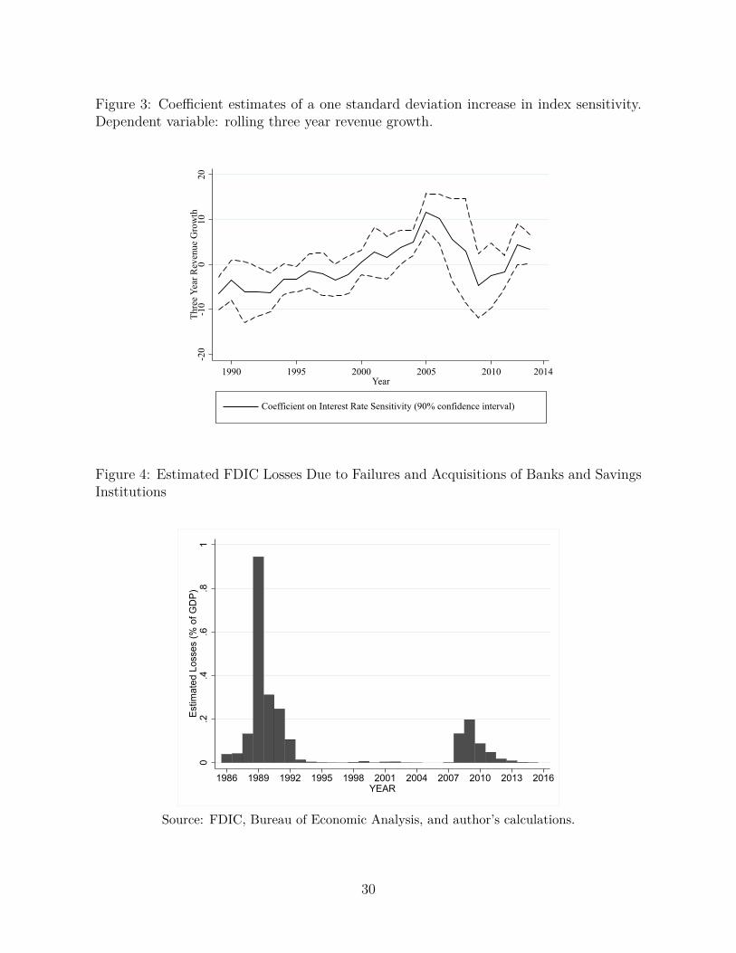
Figure 3: Coefficient estimates of a one standard deviation increase in index sensitivity.Dependent variable: rolling three year revenue growth.

-20

-10

010

20Th

ree

Year

Rev

enue

Gro

wth

1990 1995 2000 2005 2010 2014Year

Coefficient on Interest Rate Sensitivity (90% confidence interval)

Figure 4: Estimated FDIC Losses Due to Failures and Acquisitions of Banks and SavingsInstitutions

0.2

.4.6

.81

Estim

ated

Los

ses

(% o

f GD

P)

1986 1989 1992 1995 1998 2001 2004 2007 2010 2013 2016YEAR

Source: FDIC, Bureau of Economic Analysis, and author’s calculations.

30

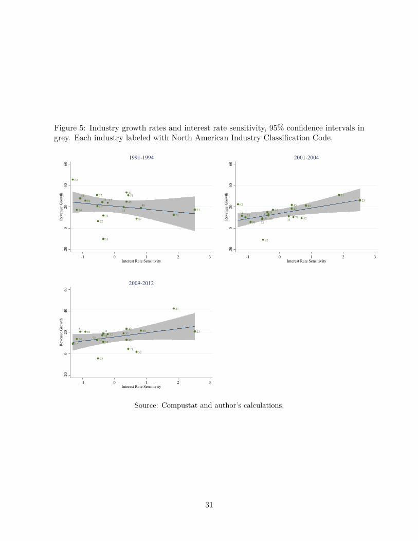
Figure 5: Industry growth rates and interest rate sensitivity, 95% confidence intervals ingrey. Each industry labeled with North American Industry Classification Code.

62

54

5181

72

56

22

44

53

31

32

33

42

45

71

52

48

21

23

-20

020

4060

Rev

enue

Gro

wth

-1 0 1 2 3Interest Rate Sensitivity

1991-1994

62

5451

81 7256

22

44

5331

32

33

4245

71 52

48

21

23

-20

020

4060

Rev

enue

Gro

wth

-1 0 1 2 3Interest Rate Sensitivity

2001-2004

6254

5181

7256

22

44

53

3132 33

42

45

7152

48

21

23

-20

020

4060

Rev

enue

Gro

wth

-1 0 1 2 3Interest Rate Sensitivity

2009-2012

Source: Compustat and author’s calculations.

31

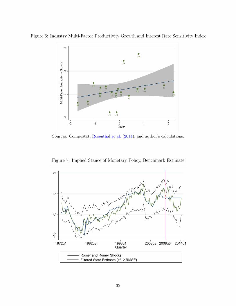
Figure 6: Industry Multi-Factor Productivity Growth and Interest Rate Sensitivity Index

2122

23

31 32

33

42

44 45

4851

52

53

54

56

62

7172

81

-.20

.2.4

Mul

ti-Fa

ctor

Pro

duct

ivity

Gro

wth

-2 -1 0 1 2Index

Sources: Compustat, Rosenthal et al. (2014), and author’s calculations.

Figure 7: Implied Stance of Monetary Policy, Benchmark Estimate

-10

-50

5

1972q1 1982q3 1993q1 2003q3 2014q12008q3Quarter

Romer and Romer ShocksFiltered State Estimate (+/- 2 RMSE)

32

Figure 8: Implied Stance of Monetary Policy: Out-of-Sample Cross-Validation

-10

-50

5

1972q1 1982q3 1993q1 2014q11999q3 2008q3Quarter

Romer and Romer ShocksFiltered State Estimate (Benchmark +/- 2 RMSE)

Estimates following 1999:Q3 are using out-of-sample VAR parameters from before that date.

Figure 9: Implied Stance of Monetary Policy: Great Moderation Data

-10

-50

5

1990q1 1995q1 2000q1 2005q1 2015q12008q3Quarter

Romer and Romer ShocksFiltered State Estimate (Benchmark +/- 2 RMSE)

33

Tabl

e1:

Mea

nIn

dust

ryR

even

ueG

row

th:

1971

:Q1-

2008

:Q3

Nam

eN

aics

Obs

Mea

nM

edia

nSD

Min

Max

Agr

icul

ture

,For

estr

y,Fi

shin

gan

dH

untin

g11

151

4.68

4.50

14.0

9-2

8.81

42.1

7M

inin

g,Q

uarr

ying

,and

Oil

and

Gas

Extr

actio

n21

151

8.10

8.84

15.3

8-4

6.51

38.5

5U

tiliti

es22

151

4.29

5.07

7.3

-27.

8429

.85

Con

stru

ctio

n23

151

4.34

4.93

11.3

2-2

4.54

29.9

8M

anuf

actu

ring

(mos

tlyno

n-du

rabl

es)

3115

13.

453.

434.

84-1

4.52

14.8

3M

anuf

actu

ring

(mos

tlyno

n-du

rabl

es)

3215

16.

767.

405.

40-1

1.17

17.1

4M

anuf

actu

ring

(mos

tlydu

rabl

es)

3315

16.

297.

117.

22-1

6.93

19.1

2W

hole

sale

Trad

e42

151

6.00

8.01

7.45

-16.

9317

.76

Ret

ailT

rade

4415

16.

887.

094.

46-5

.07

16.3

0R

etai

lTra

de45

151

8.84

8.89

7.07

-5.9

035

.57

Tran

spor

tatio

nan

dW

areh

ousin

g48

151

7.47

8.49

7.24

-15.

1729

.37

Tran

spor

tatio

nan

dW

areh

ousin

g49

151

8.40

8.28

12.2

6-1

9.84

39.4

9In

form

atio

n51

151

11.1

210

.29

8.32

-4.2

139

.44

Fina

nce

and

Insu

ranc

e52

151

6.50

6.98

8.10

-30.

3524

.76

Rea

lEst

ate

and

Ren

tala

ndLe

asin

g53

151

4.90

5.58

8.16

-13.

7623

.18

Prof

essio

nal,

Scie

ntifi

c,an

dTe

chni

calS

ervi

ces

5415

19.

559.

467.

25-8

.68

27.3

2A

dmin

istra

tive,

Supp

ort,

Was

teM

anag

emen

t/R

emed

iatio

nSe

rvic

es56

151

9.77

10.2

68.

23-1

1.44

27.1

6Ed

ucat

iona

lSer

vice

s61

151

14.4

012

.72

14.9

0-2

7.3

65.5

6H

ealth

Car

ean

dSo

cial

Ass

istan

ce62

151

15.1

115

.00

8.24

-9.9

332

.71

Art

s,En

tert

ainm

ent,

and

Rec

reat

ion

7115

110

.38

10.8

810

.82

-18.

5032

.60

Acc

omm

odat

ion

and

Food

Serv

ices

7215

16.

937.

396.

86-1

1.99

25.6

8O

ther

Serv

ices

(exc

ept

Publ

icA

dmin

istra

tion)

8115

15.

384.

749.

71-1

7.37

29.1

8To

tal

3322

7.71

7.78

9.78

-46.

5165

.56

Sour

ce:

Com

pust

atan

dau

thor

’sca

lcul

atio

ns.

34

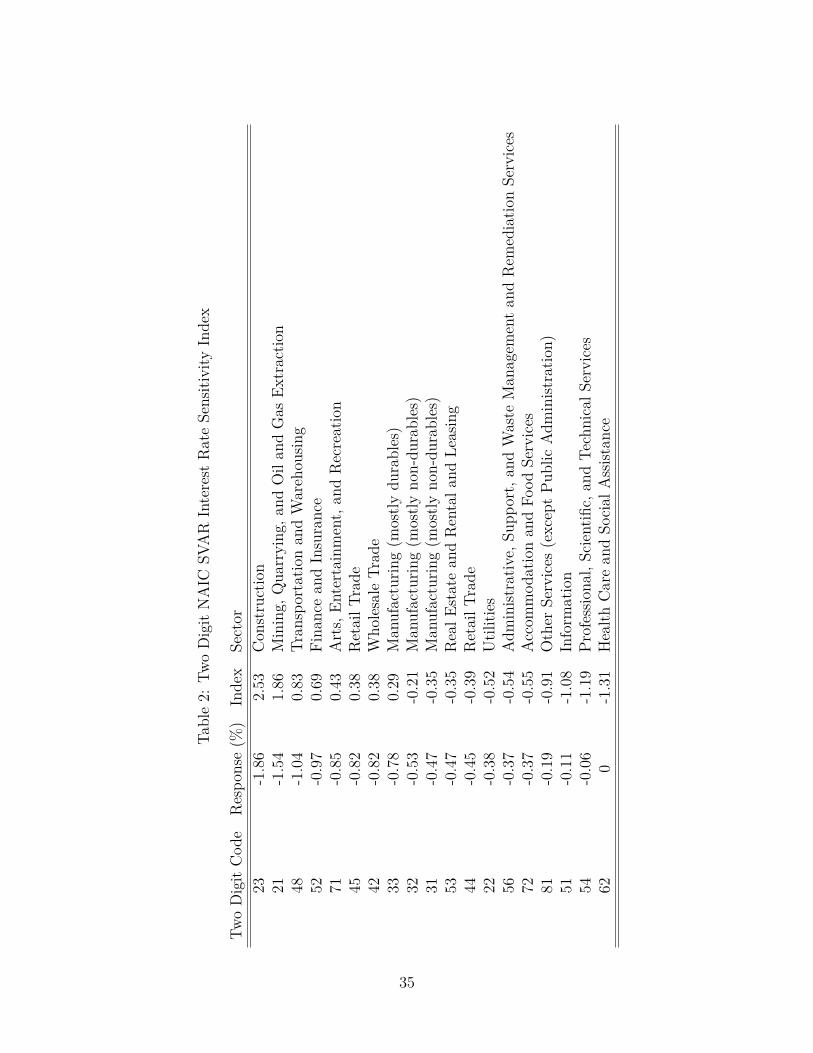
Tabl

e2:

Two

Dig

itN

AIC

SVA

RIn

tere

stR

ate

Sens

itivi

tyIn

dex

Two

Dig

itC

ode

Res

pons

e(%

)In

dex

Sect

or23

-1.8

62.

53C

onst

ruct

ion

21-1

.54

1.86

Min

ing,

Qua

rryi

ng,a

ndO

ilan

dG

asEx

trac

tion

48-1

.04

0.83

Tran

spor

tatio

nan

dW

areh

ousin

g52

-0.9

70.

69Fi

nanc

ean

dIn

sura

nce

71-0

.85

0.43

Art

s,En

tert

ainm

ent,

and

Rec

reat

ion

45-0

.82

0.38

Ret

ailT

rade

42-0

.82

0.38

Who

lesa

leTr

ade

33-0

.78

0.29

Man

ufac

turin

g(m

ostly

dura

bles

)32

-0.5

3-0

.21

Man

ufac

turin

g(m

ostly

non-

dura

bles

)31

-0.4

7-0

.35

Man

ufac

turin

g(m

ostly

non-

dura

bles

)53

-0.4

7-0

.35

Rea

lEst

ate

and

Ren

tala

ndLe

asin

g44

-0.4

5-0

.39

Ret

ailT

rade

22-0

.38

-0.5

2U

tiliti

es56

-0.3

7-0

.54

Adm

inist

rativ

e,Su

ppor

t,an

dW

aste

Man

agem

ent

and

Rem

edia

tion

Serv

ices

72-0

.37

-0.5

5A

ccom

mod

atio

nan

dFo

odSe

rvic

es81

-0.1

9-0

.91

Oth

erSe

rvic

es(e

xcep

tPu

blic

Adm

inist

ratio

n)51

-0.1

1-1

.08

Info

rmat

ion

54-0

.06

-1.1

9Pr

ofes

siona

l,Sc

ient

ific,

and

Tech

nica

lSer

vice

s62

0-1

.31

Hea

lthC

are

and

Soci

alA

ssist

ance

35

Table 3: Real Revenue Growth, Baseline Specification

(1) (2) (3) (4)Index -0.028 0.696 0.531 0.885

(1.779) (2.545) (2.361) (2.653)Index·2012 2.442 2.346 2.611 2.617

(3.692) (2.970) (3.087) (3.096)Elasticity·94 4.489** 3.943** 4.311**

(1.842) (1.718) (1.767)Elasticity·09 -0.586 -0.050 0.121

(3.628) (3.503) (3.349)Elasticity·12 1.088 0.788 1.091

(4.260) (4.149) (3.893)Emp·94 -5.874*** -5.830***

(0.954) (0.960)Emp·09 0.531 0.667

(0.675) (0.701)Emp·12 -0.027 0.080

(0.685) (0.671)Secular Trend -3.490

(5.083)1991-1994 19.222*** 12.532*** 17.787*** 20.181***

(2.146) (3.862) (3.907) (3.904)2001-2004 12.107*** 12.992* 10.295 12.699**

(1.494) (6.831) (6.557) (5.717)2009-2012 14.887*** 13.263 13.276 15.496*

(3.183) (7.984) (8.152) (8.211)

Observations 17,723 17,723 16,480 16,480Adjusted R-squared 0.068 0.069 0.067 0.068

*** p < 0.01, ** p < 0.05, * p < 0.1. Standard errors clustered at NAIC 2 digit level inparentheses.

36

Table 4: Real Revenue Growth: Pre-trends

(1) (2) (3) (4)Index -4.589 -4.932 -4.318* -3.729*

(4.145) (2.847) (2.340) (2.075)Index·2009-2009 -0.961 -2.729 -3.677 -3.693

(3.080) (2.973) (2.592) (2.548)

Observations 18,333 18,333 16,313 16,313Adjusted R-squared 0.063 0.064 0.041 0.042

**** p < 0.01, ** p < 0.05, * p < 0.1. Standard errors clustered at NAIC 2digit level in parentheses. Time indicators not shown. Column (2) controls forindustry-level GDP elasticity, column (3) controls for initial log employment,and Column (4) controls for secular industry trends as in Table 3.

Table 5: Real Revenue Growth: Controlling for Mean Reversion

(1) (2) (3) (4)Index 1.833 2.134 2.582 3.043

(1.340) (1.855) (1.822) (1.855)Index·2012 0.913 1.497 1.532 1.526

(3.139) (2.692) (2.679) (2.678)Lagged Growth 0.046*** 0.047*** 0.048*** 0.047***

(0.016) (0.016) (0.014) (0.014)

Observations 14,734 14,734 14,157 14,157Adjusted R-squared 0.041 0.042 0.053 0.054

**** p < 0.01, ** p < 0.05, * p < 0.1. Standard errors clustered at NAIC 2 digit level inparentheses. Time indicators not shown. Column (2) controls for industry-level GDPelasticity, column (3) controls for initial log employment, and Column (4) controls forsecular industry trends as in Table 3.

37

Table 6: Real Revenue Growth: BootstrappedStandard Errors Accounting for Generated Regres-sors

Clustered BootstrappedIndex 1.087

(1.701) (2.248)Index·2012 2.762

(2.947) (3.439)1991-1994 20.554***

(2.342) (2.637)2001-2004 13.827***

(2.342) (1.931)2009-2012 15.671***

(2.342) (2.208)

Observations 57 57Adjusted R-squared 0.731

*** p < 0.01, ** p < 0.05, * p < 0.1. Bootstrap proceduredescribed in text.

Table 7: Romer and Romer Alternative Shock Measures

Baseline R&R Shocks W/ NFC and Fiscal VariablesBaseline 1.00R&R 0.85 1.00R&R NFC 0.80 0.73 1.00

Column (2) uses an index measured with cumulative Romer and Romer shocks in place of thefederal funds rate. Column (3) uses the cumulative Romer and Romer shocks in place of thefederal funds rate, non-financial corporate output in place of GDP growth, includes governmentconsumption and investment ordered first, includes government tax revenues ordered second,and excludes commodity prices.

38

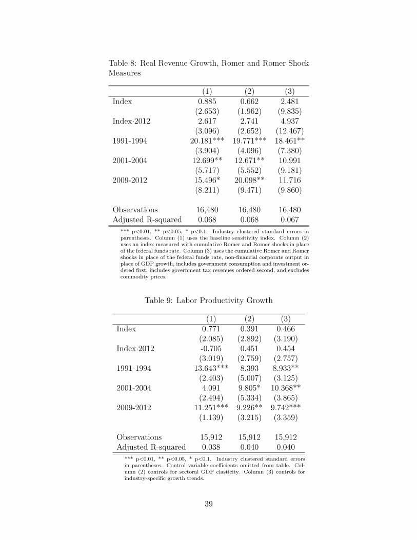
Table 8: Real Revenue Growth, Romer and Romer ShockMeasures

(1) (2) (3)Index 0.885 0.662 2.481

(2.653) (1.962) (9.835)Index·2012 2.617 2.741 4.937

(3.096) (2.652) (12.467)1991-1994 20.181*** 19.771*** 18.461**

(3.904) (4.096) (7.380)2001-2004 12.699** 12.671** 10.991

(5.717) (5.552) (9.181)2009-2012 15.496* 20.098** 11.716

(8.211) (9.471) (9.860)

Observations 16,480 16,480 16,480Adjusted R-squared 0.068 0.068 0.067

*** p<0.01, ** p<0.05, * p<0.1. Industry clustered standard errors inparentheses. Column (1) uses the baseline sensitivity index. Column (2)uses an index measured with cumulative Romer and Romer shocks in placeof the federal funds rate. Column (3) uses the cumulative Romer and Romershocks in place of the federal funds rate, non-financial corporate output inplace of GDP growth, includes government consumption and investment or-dered first, includes government tax revenues ordered second, and excludescommodity prices.

Table 9: Labor Productivity Growth

(1) (2) (3)Index 0.771 0.391 0.466

(2.085) (2.892) (3.190)Index·2012 -0.705 0.451 0.454

(3.019) (2.759) (2.757)1991-1994 13.643*** 8.393 8.933**

(2.403) (5.007) (3.125)2001-2004 4.091 9.805* 10.368**

(2.494) (5.334) (3.865)2009-2012 11.251*** 9.226** 9.742***

(1.139) (3.215) (3.359)

Observations 15,912 15,912 15,912Adjusted R-squared 0.038 0.040 0.040

*** p<0.01, ** p<0.05, * p<0.1. Industry clustered standard errorsin parentheses. Control variable coefficients omitted from table. Col-umn (2) controls for sectoral GDP elasticity. Column (3) controls forindustry-specific growth trends.

39

Table 10: Real Revenue Growth: Controlling for FiscalPolicy

(1) (2) (3)Index -0.028 0.553 0.814

(1.779) (2.309) (2.553)Index·2012 2.442 0.639 3.228

(3.692) (2.671) (2.641)FiscalIndex 2.021 1.976

(2.963) (3.561)FiscalIndex·2012 -5.808* -9.499***

(2.815) (2.697)1991-1994 19.222*** 19.068*** 22.195***

(2.146) (2.128) (7.546)2001-2004 12.107*** 11.833*** 14.105**

(1.494) (1.769) (6.374)2009-2012 14.887*** 15.191*** 8.006

(3.183) (3.061) (7.970)

Observations 17,723 17,723 16,480Adjusted R-squared 0.068 0.069 0.070

*** p < 0.01, ** p < 0.05, * p < 0.1. Standard errors clustered at NAIC 2digit level in parentheses. Column (3) controls for sectoral GDP elasticity,initial log employment, and industry-specific growth trends.

Table 11: Summary Statistics: Key Dependent Variables

Real Revenue GrowthYears Obs Mean Median Std. Dev. Min Max1991-1994 5987 19.27 15.00 59.89 -199.68 199.582001-2004 6778 12.12 11.45 60.12 -199.81 199.882009-2012 5124 15.12 13.22 52.11 -199.91 199.87

Employment Growth1991-1994 5249 13.65 8.08 56.55 -200 2002001-2004 6144 4.09 4.20 52.11 -200 2002009-2012 4668 11.26 9.01 44.21 -200 200

40

Appendix to “How Effective is Monetary Policy atthe Zero Lower Bound? Identification Through

Industry Heterogeneity”Arsenios Skaperdas

For Online Publication

Robustness

Alternative Interest Rate Sensitivity Indices

As shown in the paper, industry orthogonalized impulse responses exhibit variation atvaried quarters. I use alternative measure of index construction to test for the importanceof this variation. Table 1 reveals that constructing the index using 7 quarter structuralimpulse response point estimates, or 16 quarter cumulative responses, result in highlycorrelated industry orderings to the baseline using the minimum point estimate responses.Table 2 shows that the 2012 interest rate sensitivity coefficient interactions are in factpositive and significant in the second-stage regressions. With these definitions of interestrate sensitivity, the zero lower bound recovery is actually stronger than previous recoveriesin interest rate sensitive industries.1

The ordering of the SVARs was chosen in accordance with the literature. However,the index and the second-stage results are unaffected by ordering. Specifying the SVARsas normally recursively identified VARs, where industry revenues affect the macro vari-ables, results in a highly correlated index. Furthermore, rearranging the ordering of theVARs leaves all results unchanged. Table 3 presents the index correlations resulting fromdifferent orderings, while Table 4 presents the second stage estimates.

Table 5 presents correlations of the indices with a number of other specifications of theSVARs, while Table 6 presents the second-stage results. Column (2) includes indicatorsfor each quarter to control for any additional seasonality in the year over year growthrates. Column (3) omits commodity prices from the SVARs. Column (4) runs the SVARsand second-stage estimates including the three industries that are omitted in the paperdue to the fact that they have few firm-observations per quarter (Figure 2) and resulting

1Part of this is due to the fact that NAICS 52, Finance and Insurance, is ranked as less interest ratesensitive using the alternative measures, as this industry has an initial increase in revenues in responseto a contractionary monetary shock. Since this industry did poorly following the financial crisis, rankingit as less sensitive makes the 2012 index interaction coefficient more positive.

1

noisy time series (Figures 3). Column (5) constrains industry revenues to not affectthe macroeconomic aggregates, and with industry revenues ordered last. In all cases,the industry indices are highly correlated, and the second-stage estimates are largelyunchanged.

It is thought the transmission mechanism of monetary policy has changed throughtime, particularly since the early 1980s. In evaluating the transmission mechanism, Barthand Ramey (2002) find evidence that the cost channel of monetary policy decreasedafter the Volcker period. During the 1970s, the financial structure of credit marketswas affected by deregulation and and the regional de-segmentation of banking marketsFriedman (1986). The US exchange rate regime also moved from fixed to floating. Attimes before the 1980s, the Federal Reserve sought to directly limit the amount of banklending (Romer and Romer, 1989). Finally, the Fed also officially targeted monetaryaggregates rather than interest rates from 1979-1982. In spite of evidence for changes inthe monetary transmission mechanism, Table 5 shows that the index is still correlated(ρ = 0.66) when using only the post-1988:Q1 subsample for VAR index construction.Column (6) of Table 6 also shows the second-stage results are unaffected. In fact, usingonly more recent data for the SVAR index suggests that interest rate sensitive industrieshad greater revenue growth during the recovery at the zero lower bound.2

As a last check on the VAR results, the 2012 period compares favorable regardlessof lag length selections, though the magnitude and significance of the index coefficientdo fluctuate (Tables 7 and 8). In conclusion, the VARs are remarkably robust across allspecifications in the outcome of the industry ordering, and the second-stage results.

Further Second-Stage Robustness

The results hold using a balanced panel of firms, that is, using firms that exist in allrecovery years. This alleviates concerns associated with bias due to firm entry and exit.As shown in Table 9, the coefficient on the index from 2009-2012 is not statisticallydifferent from zero.

One possible criticism of all regressions presented thus far is that firm-level data isexamined while the index varies at only the industry level. Since only 19 industries areused, the effective sample size of the differences-in-differences estimates is more closelyapproximated as 19 for each recovery, rather than thousands of firms. Although standarderrors are clustered at the industry level, the small number of clusters means that clustered

2This is partly due to the fact that Finance and Insurance is ranked much less sensitive in thepost-1988 subsample, and this industry, as expected, fared poorly following the financial crisis.

2

standard errors may overstate significance.One way to evaluate whether this problem has merit is to take industry averages,

and completely ignore the firm dimension in the differences-in-differences specification.Table 10 presents the results from this process. The coefficients on the index recoveryinteractions give similar estimates. In addition, the R2 increases to 70 − 73% from the7 − 8% observed in baseline firm-level regressions.

The 2009-2012 results compare favorably to previous recoveries when dropping in-dustries one at a time (Table 11), though dropping Mining, Quarrying, and Oil and GasExtraction (21) does decrease the zero lower bound coefficient. However, it is still not sta-tistically different from previous recoveries. In addition, it is of note that when droppingthe financial industry (NAIC 52), the 2009-2012 period is characterized by significantlygreater revenue growth in interest rate sensitive industries. This is notable, as we wouldexpect the financial industry to recover slowly after the financial crisis; one could makethe case that dropping the financial industry would be more sensible for the entire pa-per. In that case, most regressions would show increased growth of interest rate sensitiveindustries at the zero lower bound.

VAR Results for Identifying the Policy Stance and In-dustry Effects of Fiscal Policy

Figure 4 presents the industry responses to a monetary shock from VARs with cumulativeRomer and Romer shocks in place of the federal funds rate, as described in Section 7 ofthe paper. These VARs are used for identifying the policy stance and for identifyingindustry senstivity to fiscal policy. Macro aggregate responses, shown in Figure 5, areas expected, with the exception of counterintuitive responses to tax shocks.3 However,the estimated Kalman filtered R&R shocks are similar when omitting tax revenues fromthe VAR. 4 Figure 6 presents the industry responses to a government spending shock,while Table 12 presents the resulting index based on Figure 6’s standardized cumulativeimpulse responses.

3VARs with government spending, tax receipts, and GDP growth over this time period result insimilar impulse responses.

4Ilzetzki (2011) also finds similar results whether controlling or not for tax revenues in VARs esti-mating effects of fiscal spending.

3

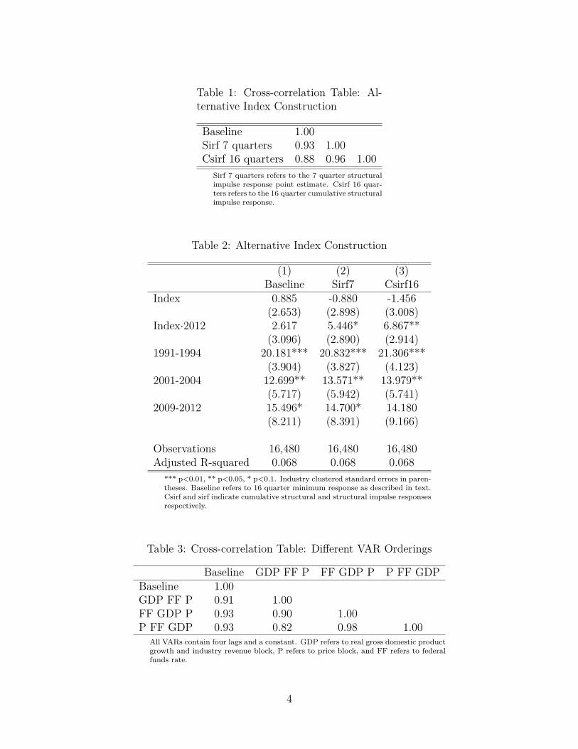
Table 1: Cross-correlation Table: Al-ternative Index Construction

Baseline 1.00Sirf 7 quarters 0.93 1.00Csirf 16 quarters 0.88 0.96 1.00

Sirf 7 quarters refers to the 7 quarter structuralimpulse response point estimate. Csirf 16 quar-ters refers to the 16 quarter cumulative structuralimpulse response.

Table 2: Alternative Index Construction

(1) (2) (3)Baseline Sirf7 Csirf16

Index 0.885 -0.880 -1.456(2.653) (2.898) (3.008)

Index·2012 2.617 5.446* 6.867**(3.096) (2.890) (2.914)

1991-1994 20.181*** 20.832*** 21.306***(3.904) (3.827) (4.123)

2001-2004 12.699** 13.571** 13.979**(5.717) (5.942) (5.741)

2009-2012 15.496* 14.700* 14.180(8.211) (8.391) (9.166)

Observations 16,480 16,480 16,480Adjusted R-squared 0.068 0.068 0.068

*** p<0.01, ** p<0.05, * p<0.1. Industry clustered standard errors in paren-theses. Baseline refers to 16 quarter minimum response as described in text.Csirf and sirf indicate cumulative structural and structural impulse responsesrespectively.

Table 3: Cross-correlation Table: Different VAR Orderings

Baseline GDP FF P FF GDP P P FF GDPBaseline 1.00GDP FF P 0.91 1.00FF GDP P 0.93 0.90 1.00P FF GDP 0.93 0.82 0.98 1.00

All VARs contain four lags and a constant. GDP refers to real gross domestic productgrowth and industry revenue block, P refers to price block, and FF refers to federalfunds rate.

4

Table 4: Real Revenue Growth, Different VAR Orderings

(1) (2) (3) (4)Baseline GDP FF P FF GDP P P FF GDP

Index 0.885 0.348 0.155 0.030(2.653) (2.759) (2.468) (2.420)

Index·2012 2.617 3.437 6.451** 6.840***(3.096) (3.136) (2.267) (2.370)

1991-1994 20.181*** 20.501*** 20.354*** 20.476***(3.904) (4.131) (3.978) (4.092)

2001-2004 12.699** 13.115** 12.999** 13.125**(5.717) (5.722) (5.775) (5.875)

2009-2012 15.496* 16.908* 13.001* 11.095(8.211) (8.906) (7.361) (7.189)

Observations 16,480 16,480 16,480 16,480Adjusted R-squared 0.068 0.068 0.069 0.069

*** p<0.01, ** p<0.05, * p<0.1*** p<0.01, ** p<0.05, * p<0.1. Industry standard errors clustered in parentheses.

Table 5: Cross-correlation Table: Alternative Specifications

Baseline Qrtr Ind No Com Post-1988Baseline 1.00Quarter Indicators 1.00 1.00No Commodity Prices 0.98 0.97 1.00Post-1988 0.66 0.64 0.65 1.00

5

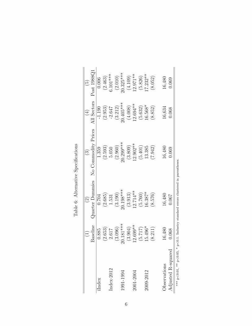
Tabl

e6:

Alte

rnat

ive

Spec

ifica

tions

(1)

(2)

(3)

(4)

(5)

Base

line

Qua

rter

Dum

mie

sN

oC

omm

odity

Pric

esA

llSe

ctor

sPo

st19

88Q

1iIn

dex

0.88

50.

704

1.35

9-1

.190

0.00

6(2

.653

)(2

.685

)(2

.593

)(2

.953

)(2

.463

)In

dex·

2012

2.61

71.

531

5.05

0-2

.647

6.10

1***

(3.0

96)

(3.1

90)

(2.9

60)

(3.2

12)

(2.0

10)

1991

-199

420

.181

***

20.1

98**

*20

.299

***

20.4

05**

*20

.325

***

(3.9

04)

(3.9

13)

(3.8

09)

(4.0

08)

(4.1

09)

2001

-200

412

.699

**12

.714

**12

.902

**12

.694

**12

.971

**(5

.717

)(5

.760

)(5

.401

)(5

.632

)(5

.826

)20

09-2

012

15.4

96*

16.3

87*

13.3

8516

.568

*17

.232

**(8

.211

)(8

.576

)(7

.942

)(8

.852

)(8

.052

)

Obs

erva

tions

16,4

8016

,480

16,4

8016

,634

16,4

80A

djus

ted

R-s

quar

ed0.

068

0.06

70.

069

0.06

80.

069

***

p<0.

01,*

*p<

0.05

,*p<

0.1.

Indu

stry

stan

dard

erro

rscl

uste

red

inpa

rent

hese

s.

6

Table 7: Cross-correlation Table: AlternativeLag Lengths

Baseline 2 Lags 3 Lags 5 LagsBaseline 1.002 Lags 0.94 1.003 Lags 0.96 0.96 1.005 Lags 0.93 0.90 0.93 1.00

7

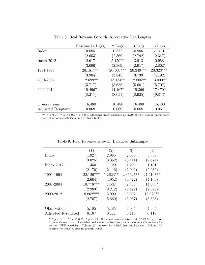
Table 8: Real Revenue Growth, Alternative Lag Lengths

Baseline (4 Lags) 2 Lags 3 Lags 5 LagsIndex 0.885 0.337 0.906 -0.431

(2.653) (2.369) (2.792) (2.347)Index·2012 2.617 5.450** 3.513 0.958

(3.096) (2.369) (2.917) (2.802)1991-1994 20.181*** 20.500*** 20.249*** 20.323***

(3.904) (3.845) (3.739) (4.192)2001-2004 12.699** 13.134** 12.806** 13.090**

(5.717) (5.688) (5.601) (5.707)2009-2012 15.496* 14.167* 15.366 17.470*

(8.211) (8.051) (8.925) (9.813)

Observations 16,480 16,480 16,480 16,480Adjusted R-squared 0.068 0.069 0.068 0.067

*** p < 0.01, ** p < 0.05, * p < 0.1. Standard errors clustered at NAIC 2 digit level in parentheses.Control variable coefficients omitted from table.

Table 9: Real Revenue Growth, Balanced Subsample

(1) (2) (3) (4)Index 1.927 2.985 2.689 3.058

(3.025) (3.362) (3.111) (2.674)Index·2012 1.450 1.129 1.299 1.181

(2.170) (2.116) (2.042) (2.082)1991-1994 22.126*** 13.623** 20.162*** 27.410***

(2.604) (4.952) (4.572) (4.169)2001-2004 10.778*** 7.537 7.480 14.600*

(2.983) (9.212) (9.472) (7.028)2009-2012 8.862*** 5.900 5.592 12.620**

(2.707) (5.660) (6.067) (5.398)

Observations 5,185 5,185 4,965 4,965Adjusted R-squared 0.107 0.111 0.113 0.118

*** p < 0.01, ** p < 0.05, * p < 0.1. Standard errors clustered at NAIC 2 digit levelin parentheses. Control variable coefficients omitted from table. Column (2) controls forsectoral GDP elasticity. Column (3) controls for initial firm employment. Column (4)controls for industry-specific growth trends.

8

Table 10: Real Revenue Growth, Industry-Level Data

(1) (2) (3) (4)Index 1.087 1.398 1.615 1.643

(1.701) (1.774) (1.829) (1.857)Index·2012 2.762 2.344 2.233 2.260

(2.947) (3.073) (3.228) (3.267)1991-1994 20.554*** 16.403*** 9.882 10.328

(2.342) (4.485) (7.427) (7.977)2001-2004 13.827*** 13.630*** 14.007* 14.196*

(2.342) (4.485) (7.812) (7.979)2009-2012 15.671*** 16.424*** 15.503* 15.679*

(2.342) (4.524) (7.859) (8.014)

Observations 57 57 57 57Adjusted R-squared 0.731 0.721 0.711 0.705

*** p < 0.01, ** p < 0.05, * p < 0.1. Standard errors clustered at NAIC 2 digit level inparentheses. Control variable coefficients omitted from table. Column (2) controls forsectoral GDP elasticity. Column (3) controls for initial firm employment. Column (4)controls for industry-specific growth trends.

9

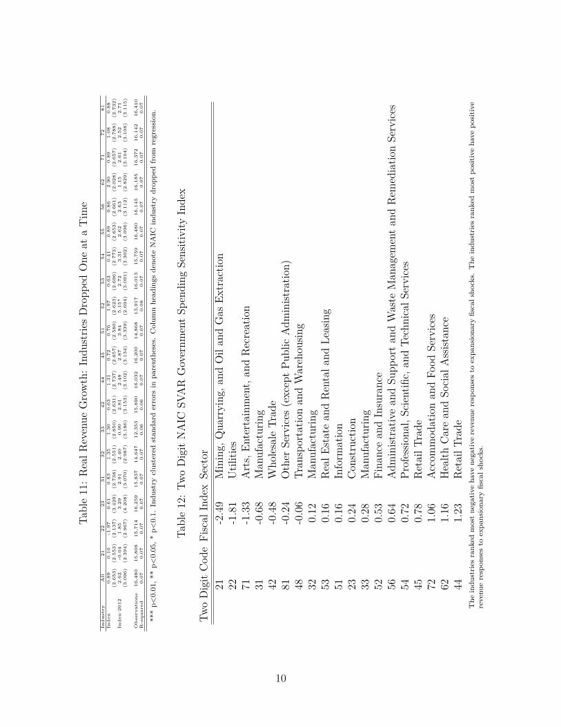
Tabl

e11

:R

ealR

even

ueG

row

th:

Indu

strie

sD

ropp

edO

neat

aT

ime

Ind

ust

ryA

ll21

2223

3132

3342

4445

5152

5354

5556

6271

7281

Ind

ex0.

890.

10-1

.97

0.61

0.83

1.35

1.30

0.63

1.31

0.72

0.76

1.97

0.63

0.41

0.89

0.86

2.90

0.89

1.08

0.88

(2.6

53)

(2.5

53)

(2.1

37)

(3.4

29)

(2.7

38)

(2.5

51)

(2.8

50)

(2.6

31)

(2.7

37)

(2.6

57)

(2.5

80)

(2.6

23)

(2.6

96)

(2.7

73)

(2.6

53)

(2.6

61)

(2.0

28)

(2.6

57)

(2.7

88)

(2.7

32)

Ind

ex·2

012

2.62

-0.0

41.

853.

292.

912.

400.

902.

812.

482.

873.

845.

15*

2.72

3.31

2.62

2.63

1.15

2.61

2.52

2.71

(3.0

96)

(2.3

94)

(2.9

67)

(4.2

08)

(3.0

70)

(2.9

87)

(3.1

86)

(3.1

53)

(3.1

02)

(3.1

34)

(3.3

39)

(2.6

94)

(3.0

91)

(3.3

02)

(3.0

96)

(3.1

12)

(2.8

29)

(3.1

04)

(3.1

08)

(3.1

15)

Ob

serv

atio

ns

16,4

8015

,808

15,7

1416

,259

15,8

3714

,647

12,3

5315

,890

16,0

3216

,200

14,8

6813

,917

16,0

1315

,759

16,4

8016

,145

16,1

8516

,372

16,1

4216

,410

R-s

qu

ared

0.07

0.07

0.07

0.07

0.07

0.07

0.06

0.06

0.07

0.07

0.07

0.08

0.07

0.07

0.07

0.07

0.07

0.07

0.07

0.07

***

p<0.

01,*

*p<

0.05

,*p<

0.1.

Indu

stry

clus

tere

dst

anda

rder

rors

inpa

rent

hese

s.C

olum

nhe

adin

gsde

note

NA

ICin

dust

rydr

oppe

dfr

omre

gres

sion

.

Tabl

e12

:Tw

oD

igit

NA

ICSV

AR

Gov

ernm

ent

Spen

ding

Sens

itivi

tyIn

dex

Two

Dig

itC

ode

Fisc

alIn

dex

Sect

or21

-2.4

9M

inin

g,Q

uarr

ying

,and

Oil

and

Gas

Extr

actio

n22

-1.8

1U

tiliti

es71

-1.3

3A

rts,

Ente

rtai

nmen

t,an

dR

ecre

atio

n31

-0.6

8M

anuf

actu

ring

42-0

.48

Who

lesa

leTr

ade

81-0

.24

Oth

erSe

rvic

es(e

xcep

tPu

blic

Adm

inist

ratio

n)48

-0.0

6Tr

ansp

orta

tion

and

War

ehou

sing

320.

12M

anuf

actu

ring

530.

16R

ealE

stat

ean

dR

enta

land

Leas

ing

510.

16In

form

atio

n23

0.24

Con

stru

ctio

n33

0.28

Man

ufac

turin

g52

0.53

Fina

nce

and

Insu

ranc

e56

0.64

Adm

inist

rativ

ean

dSu

ppor

tan

dW

aste

Man

agem

ent

and

Rem

edia

tion

Serv

ices

540.

72Pr

ofes

siona

l,Sc

ient

ific,

and

Tech

nica

lSer

vice

s45

0.78

Ret

ailT

rade

721.

06A

ccom

mod

atio

nan

dFo

odSe

rvic

es62

1.16

Hea

lthC

are

and

Soci

alA

ssist

ance

441.

23R

etai

lTra

deT

hein

dust

ries

rank

edm

ost

nega

tive

have

nega

tive

reve

nue

resp

onse

sto

expa

nsio

nary

fisca

lsho

cks.

The

indu

stri

esra

nked

mos

tpo

siti

veha

vepo

siti

vere

venu

ere

spon

ses

toex

pans

iona

ryfis

cals

hock

s.

10

Figure 1: Quarterly Industry Revenues: 2005Q1-2008Q3.

050

100

150

Num

ber o

f Qua

rterly

Obs

erva

tions

0 .02 .04 .06 .08Industry Revenues as a Fraction of Gross Output

This figure shows that individual industry revenues tend to be a small portion of aggregaterevenues. Sources: Compustat, Bureau of Economic Analysis, and author’s calculations.

11

Figure 2: Average Number of Quarterly Firm Observations by North American IndustrialClassification Code, 1970:Q1-2008:Q3

050

01,

000

1,50

0N

umbe

r of F

irm O

bser

vatio

ns

11 21 22 23 31 32 33 42 44 45 48 49 51 52 53 54 56 61 62 71 72 81North American Industrial Classification Code

Source: Compustat and author’s calculations.

12

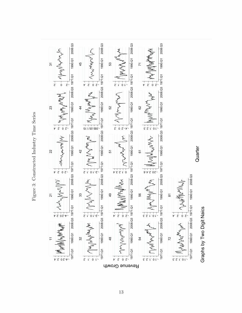
Figu

re3:

Con

stru

cted

Indu

stry

Tim

eSe

ries

-.4-.20.2.4

-.4-.20.2.4

-.20.2.4

-.20.2.4

-.20.2

-.10.1.2

-.2-.10.1.2

-.2-.10.1.2

-.050.05.1.15

-.20.2.4

-.20.2.4

-.20.2.4

0.1.2.3.4

-.4-.20.2

-.10.1.2

-.10.1.2.3

-.10.1.2.3

-.20.2.4.6

-.10.1.2.3

-.20.2.4

-.10.1.2.3

-.20.2.4

1971

:Q1

1990

:Q1

2008

:Q3

1971

:Q1

1990

:Q1

2008

:Q3

1971

:Q1

1990

:Q1

2008

:Q3

1971

:Q1

1990

:Q1

2008

:Q3

1971

:Q1

1990

:Q1

2008

:Q3

1971

:Q1

1990

:Q1

2008

:Q3

1971

:Q1

1990

:Q1

2008

:Q3

1971

:Q1

1990

:Q1

2008

:Q3

1971

:Q1

1990

:Q1

2008

:Q3

1971

:Q1

1990

:Q1

2008

:Q3

1971

:Q1

1990

:Q1

2008

:Q3

1971

:Q1

1990

:Q1

2008

:Q3

1971

:Q1

1990

:Q1

2008

:Q3

1971

:Q1

1990

:Q1

2008

:Q3

1971

:Q1

1990

:Q1

2008

:Q3

1971

:Q1

1990

:Q1

2008

:Q3

1971

:Q1

1990

:Q1

2008

:Q3

1971

:Q1

1990

:Q1

2008

:Q3

1971

:Q1

1990

:Q1

2008

:Q3

1971

:Q1

1990

:Q1

2008

:Q3

1971

:Q1

1990

:Q1

2008

:Q3

1971

:Q1

1990

:Q1

2008

:Q3

1121

2223

31

3233

4244

45

4849

5152

53

5456

6162

71

7281

Revenue Growth

Qua

rter

Gra

phs

by T

wo

Dig

it N

aics

13

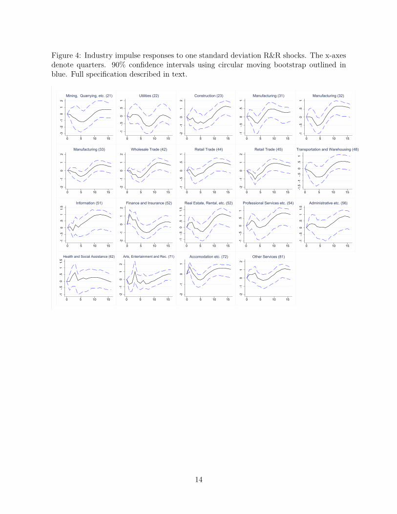
Figure 4: Industry impulse responses to one standard deviation R&R shocks. The x-axesdenote quarters. 90% confidence intervals using circular moving bootstrap outlined inblue. Full specification described in text.

-3-2

-10

12

0 5 10 15

Mining, Quarrying, etc. (21)

-1-.5

0.5

1

0 5 10 15

Utilities (22)

-2-1

01

2

0 5 10 15

Construction (23)

-1-.5

0.5

1

0 5 10 15

Manufacturing (31)

-1-.5

0.5

1

0 5 10 15

Manufacturing (32)

-2-1

01

2

0 5 10 15

Manufacturing (33)

-2-1

01

2

0 5 10 15

Wholesale Trade (42)

-1-.5

0.5

1

0 5 10 15

Retail Trade (44)

-2-1

01

2

0 5 10 15

Retail Trade (45)

-1.5

-1-.5

0.5

1

0 5 10 15

Transportation and Warehousing (48)

-1-.5

0.5

11.

5

0 5 10 15

Information (51)

-2-1

01

2

0 5 10 15

Finance and Insurance (52)

-1-.5

0.5

11.

5

0 5 10 15

Real Estate, Rental, etc. (52)

-1-.5

0.5

1

0 5 10 15

Professional Services etc. (54)

-1-.5

0.5

11.

5

0 5 10 15

Administrative etc. (56)

-1-.5

0.5

11.

5

0 5 10 15

Health and Social Assistance (62)

-2-1

01

2

0 5 10 15

Arts, Entertainment and Rec. (71)

-2-1

01

0 5 10 15

Accomodation etc. (72)

-2-1

01

2

0 5 10 15

Other Services (81)

14

Figure 5: Aggregate impulse responses to one standard deviation shocks using R&RShocks. The x-axes denote quarters. 90% confidence intervals using circular movingbootstrap outlined in blue. Charts labeled by impulse, response. Full specification de-scribed in text.

0.5

1

0 5 10 15

Govt Cons, Govt Cons

-.50

.5

0 5 10 15

Govt Cons, Taxes-.4

-.20

.2.4

0 5 10 15

Govt Cons, NFC Output

-.6-.4

-.20

.2

0 5 10 15

Govt Cons, PCE Inflation

-.05

0.0

5.1

.15

.2

0 5 10 15

Govt Cons, R&R Shocks

-.4-.2

0.2

0 5 10 15

Taxes, Govt Cons

-.50

.51

1.5

2

0 5 10 15

Taxes, Taxes

-.50

.51

0 5 10 15

Taxes, NFC Output

-.20

.2.4

0 5 10 15

Taxes, PCE Inflation

-.1-.0

50

.05

.1

0 5 10 15

Taxes, R&R Shocks

-.20

.2.4

0 5 10 15

NFC Output, Govt Cons

-1-.5

0.5

1

0 5 10 15

NFC Output, Taxes

-1-.5

0.5

11.

5

0 5 10 15

NFC Output, NFC Output

-.4-.2

0.2

.4

0 5 10 15

NFC Output, PCE Inflation

-.1-.0

50

.05

.1.1

50 5 10 15

NFC Output, R&R Shocks

-.2-.1

0.1

.2

0 5 10 15

PCE Inflation, Govt Cons

-1-.5

0.5

0 5 10 15

PCE Inflation, Taxes

-1-.5

0.5

0 5 10 15

PCE Inflation, NFC Output

-.20

.2.4

.6

0 5 10 15

PCE Inflation, PCE Inflation-.2

-.10

.1.2

0 5 10 15

PCE Inflation, R&R Shocks

-.20

.2.4

0 5 10 15

R&R Shocks, Govt Cons

-1-.5

0.5

1

0 5 10 15

R&R Shocks, Taxes

-1-.5

0.5

0 5 10 15

R&R Shocks, NFC Output

-.6-.4

-.20

0 5 10 15

R&R Shocks, PCE Inflation

0.2

.4.6

0 5 10 15

R&R Shocks, R&R Shocks

15

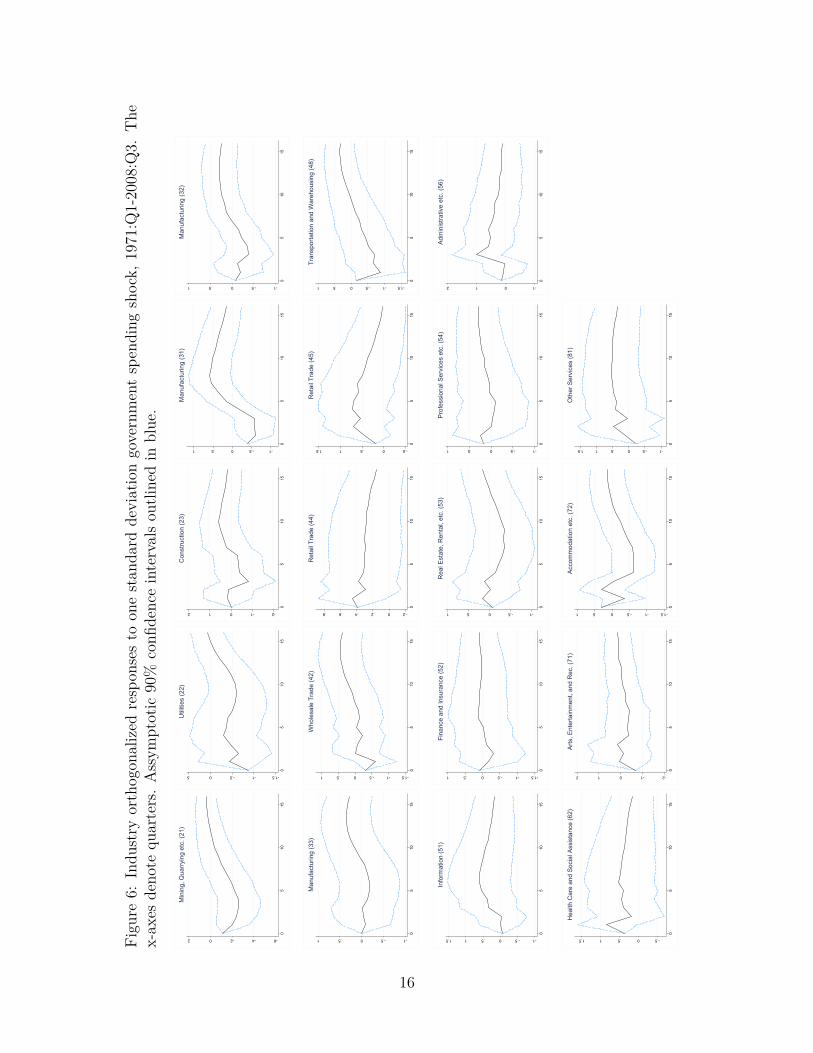
Figu

re6:

Indu

stry

orth

ogon

aliz

edre

spon

ses

toon

est

anda

rdde

viat

ion

gove

rnm

ent

spen

ding

shoc

k,19

71:Q

1-20

08:Q

3.T

hex-

axes

deno

tequ

arte

rs.

Ass

ympt

otic

90%

confi

denc

ein

terv

als

outli

ned

inbl

ue.

-6-4-202

05

1015

Min

ing,

Qua

rryin

g et

c. (2

1)

-1.5-1-.50.5

05

1015

Util

ities

(22)

-2-1012

05

1015

Con

stru

ctio

n (2

3)

-1-.50.51

05

1015

Man

ufac

turin

g (3

1)

-1-.50.51

05

1015

Man

ufac

turin

g (3

2)

-1-.50.51

05

1015

Man

ufac

turin

g (3

3)

-1.5-1-.50.51

05

1015

Who

lesa

le T

rade

(42)

-.20.2.4.6.8

05

1015

Ret

ail T

rade

(44)

-.50.511.5

05

1015

Ret

ail T

rade

(45)

-1.5-1-.50.51

05

1015

Tran

spor

tatio

n an

d W

areh

ousi

ng (4

8)

-1-.50.511.5

05

1015

Info

rmat

ion

(51)

-1.5-1-.50.51

05

1015

Fina

nce

and

Insu

ranc

e (5

2)-1-.50.51

05

1015

Rea

l Est

ate,

Ren

tal,

etc.

(53)

-1-.50.51

05

1015

Prof

essi

onal

Ser

vice

s et

c. (5

4)

-1012

05

1015

Adm

inis

trativ

e et

c. (5

6)

-.50.511.5

05

1015

Hea

lth C

are

and

Soci

al A

ssis

tanc

e (6

2)

-2-1012

05

1015

Arts

, Ent

erta

inm

ent,

and

Rec

. (71

)

-1.5-1-.50.51

05

1015

Acco

mm

odat

ion

etc.

(72)

-1-.50.511.5

05

1015

Oth

er S

ervi

ces

(81)

16

ReferencesBarth, M. J. and Ramey, V. A. (2002). The Cost Channel of Monetary Transmission.

In NBER Macroeconomics Annual 2001, Volume 16, NBER Chapters, pages 199–256.National Bureau of Economic Research, Inc.

Friedman, B. M. (1986). Money, credit, and interest rates in the business cycle. In TheAmerican business cycle: Continuity and change, pages 395–458. University of ChicagoPress.

Ilzetzki, E. (2011). Fiscal policy and debt dynamics in developing countries. World BankPolicy Research Working Paper Series, Vol.

Romer, C. D. and Romer, D. H. (1989). Does monetary policy matter? a new test in thespirit of friedman and schwartz. In NBER Macroeconomics Annual 1989, Volume 4,pages 121–184. MIT Press.

17