how forced displacements caused by a violent conflict ...ftp.iza.org/dp9926.pdf ·...
TRANSCRIPT

Forschungsinstitut zur Zukunft der ArbeitInstitute for the Study of Labor
DI
SC
US
SI
ON
P
AP
ER
S
ER
IE
S
How Forced Displacements Caused by a Violent Conflict Affect Wages in Colombia
IZA DP No. 9926
May 2016
J. Ignacio Gimenez-NadalJosé Alberto MolinaEdgar Silva Quintero
How Forced Displacements Caused by a
Violent Conflict Affect Wages in Colombia
J. Ignacio Gimenez-Nadal University of Zaragoza,
BIFI and CTUR
José Alberto Molina
University of Zaragoza, BIFI and IZA
Edgar Silva Quintero
University of Zaragoza
Discussion Paper No. 9926 May 2016
IZA
P.O. Box 7240 53072 Bonn
Germany
Phone: +49-228-3894-0 Fax: +49-228-3894-180
E-mail: [email protected]
Any opinions expressed here are those of the author(s) and not those of IZA. Research published in this series may include views on policy, but the institute itself takes no institutional policy positions. The IZA research network is committed to the IZA Guiding Principles of Research Integrity. The Institute for the Study of Labor (IZA) in Bonn is a local and virtual international research center and a place of communication between science, politics and business. IZA is an independent nonprofit organization supported by Deutsche Post Foundation. The center is associated with the University of Bonn and offers a stimulating research environment through its international network, workshops and conferences, data service, project support, research visits and doctoral program. IZA engages in (i) original and internationally competitive research in all fields of labor economics, (ii) development of policy concepts, and (iii) dissemination of research results and concepts to the interested public. IZA Discussion Papers often represent preliminary work and are circulated to encourage discussion. Citation of such a paper should account for its provisional character. A revised version may be available directly from the author.
IZA Discussion Paper No. 9926 May 2016
ABSTRACT
How Forced Displacements Caused by a Violent Conflict Affect Wages in Colombia*
In this paper, we analyze how forced displacements caused by violent conflicts affect the wages of displaced workers in Colombia, a country characterized by a long historical prevalence of violent conflicts between the government, the militia group (FARC), drug trafficking, and other crime that affect hundreds of people, forcibly displaced to other regions of the country. Using data from the Quality of Life Survey (2011-2014), we analyze differences in wages between those who were forced to move to other regions, and those who were not forced to move. In our empirical strategy, we take into account that those who were displaced may have characteristics that differ from those who were not forced, and we apply Propensity Score Matching techniques to consider forced displacements exogenous to the individuals. We apply different matching algorithms, and find that forced displacement decreases between 6% and the 22% the wages of males, and between 17% and 37% the wages of females, compared to their non-displaced counterparts. Thus, forced displacements result in poorer labor market outcomes, and the government should explore how public policies may help to alleviate the negative consequences of forced displacements as first step to reduce wage inequalities originated by these conflicts. JEL Classification: J15, J31, R23 Keywords: forced displacement, wages, Propensity Score Matching, Colombia Corresponding author: J. Ignacio Gimenez Nadal Department of Economic Analysis Faculty of Economics and Business University of Zaragoza C/ Gran Via 2 50005 Zaragoza Spain E-mail: [email protected]
* This paper has benefited from funding from the Spanish Ministry of Economics (Project ECO2012-34828).
1
1. INTRODUCTION
In this paper, we analyze how the forced displacement of individuals through violent conflicts
affect the wages of workers in Colombia. This phenomenon in Colombia has, for several
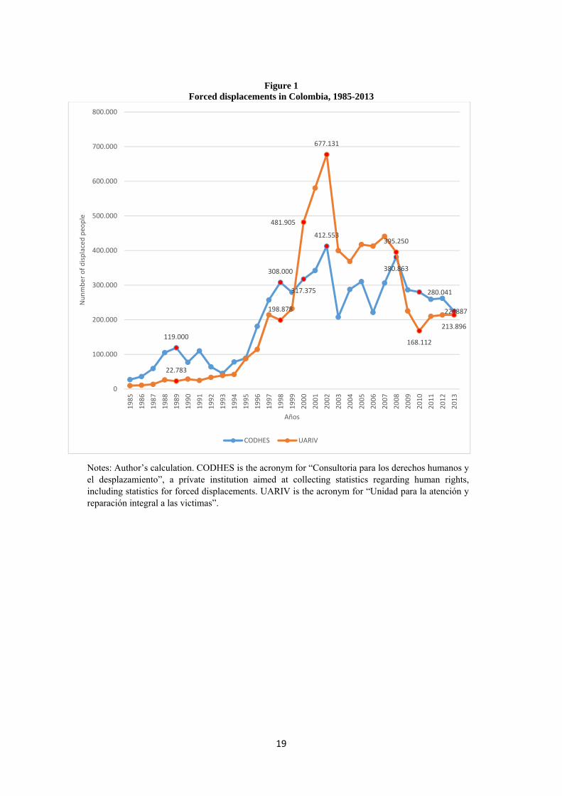
decades, attracted the attention of researchers for its importance and prevalence. Figure 1 shows
the number of such displacements in Colombia in the period (1985-2010), and we can observe
that this phenomenon is far from abating, with large numbers of displacements continuing to
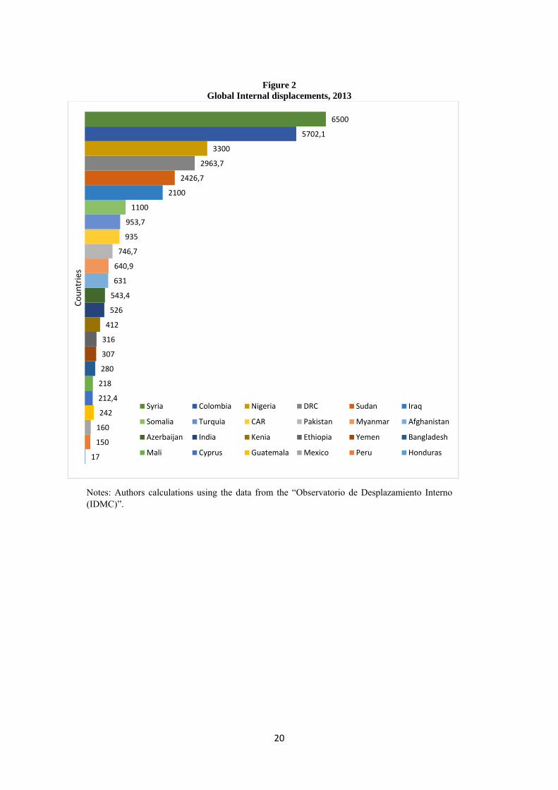
occur each year. It is also a phenomenon of global concern, given that, in the year 2013,
Colombia ranks in the second position regarding the number of displaced individuals (5.7
million of displaced people) exceeded only by Syria (6.5 million), as shown in Figure 2. As
argued by Ibañez (2009), the phenomenon involves all of Colombia's territory and nearly 90
percent of the country's municipalities either expel or receive populations. In contrast to other
countries, forced migration in Colombia is largely internal. Illegal armed groups are the primary
responsible parties, and these migrations do not result in massive refugee streams, but rather
occur on an individual basis, and the displaced population is dispersed throughout the territory
and not focused on refugee camps. Following Blattman and Miguel (2009), these characteristics
pose unique challenges for crafting state policy that can effectively mitigate the impact of
displacement, and an analysis of the economic consequences of this phenomenon may help to
guide public policies aimed at minimizing the negative consequences.
Prior research has analyzed the relationship between violent conflicts and economic
outcomes. Abadie and Gardeazabal (2003) focus their analysis on the macroeconomic
consequences of the Basque conflict in Spain, and find that, after the outbreak of terrorism in
the late 1960's, per capita GDP in the Basque Country declined by about 10 percentage points,
while firms showed a positive relative performance when the truce became credible, and a
negative relative performance at the end of the cease-fire. Angrist and Kugler (2008) analyze
the economic and social consequences of a major shift in the production of coca paste from
Peru and Bolivia to Colombia, and find that this shift generated economic gains in rural areas,
primarily in the form of increased self-employment earnings and the increased labor supply of
teenage boys, while the rural areas which saw accelerated coca production subsequently became
much more violent. Engel and Ibañez (2007) develop a conceptual framework for the empirical
analysis of displacement decisions, and apply the framework to the case of Colombia. Ibáñez
and Velásquez (2008) analyze the impact on the economic conditions of displaced workers in
Colombia, and find that labor income sharply falls after the displacement. Dube and Vargas
2
(2013) analyze how income shocks affect the armed conflict, showing that price shocks in
natural resources affect conflict in different directions, depending on the particular commodity.
If individuals are forcibly displaced to a different region of residence, their economic
outcomes will be affected. One of the most important of these outcomes is wages, consistent
with prior evidence shown by Blattman and Miguel (2010), who find that wars and civil
conflicts produce displacements of the population, which in turn produces shocks in labor
markets. If individuals are forcibly displaced, they may have problems in accessing a new
employment, given that their social networks are reduced (Sanders and Nee, 1996; Mouw,
2003, Castilla, 2005), or their wages may be lower, reflecting a mismatch between their specific
skills and the jobs available in the region (Jacobson, LaLonde and Sullivan, 1993; Eliason and
Storrie, 2006; Couch and Placzek, 2010; Hijzen, Upward and Wright, 2010; Schmieder, von
Wachter and Bender, 2010; Bonikowska and Morissette, 2012; Seim, 2012). Thus, to the extent
that displaced workers may have poorer economic outcomes, we may see violent conflicts and
their associated displacement flows as a source of inequality. Thus, the analysis of how forced
displacements affect wages of displaced workers is important for policy issues.
Using the data offered by the Quality of Life Survey (QLS) in Colombia for the years 2011
to 2014, we compare the wages of those who were forced to abandon their place of residence
through problems of violence, with those who were not forced to do so. We consider this forced
displacement as a “quasi-policy”, given that individuals who were displaced could not choose
the level of violence in their regions of origin, and we assume this displacement is an exogenous
treatment of individuals in their regions of origin. Under this assumption, we apply Propensity
Score Matching (PSM) techniques typically applied to evaluate employment and education
programs (Rosenbaum and Rubin, 1983: Lalonde, 1986; Fraker and Maynard, 1987; Heckman,
Ichimura and Todd, 1998; Dehejia and Wahba, 1999; 2002), and we find that forced
displacement decreases between 6% and 22% of the wages of males, and between 17% and
37% of the wages of females, compared to their non-displaced counterparts. These results are
consistent with existing evidence showing that the earnings and wages of displaced workers are
10-15% below their expected levels (Jacobson, LaLonde and Sullivan, 1993; Eliason and
Storrie, 2006; Couch and Placzek, 2010; Hijzen, Upward and Wright, 2010; Schmieder, von
Wachter and Bender, 2010; Bonikowska and Morissette, 2012; Seim, 2012), and we find that
forced displacement represents an important source of inequality.
3
Our contribution to the literature is twofold. First, we contribute to the analysis of the
negative economic consequences of armed conflicts (Merteens and Stoller, 2001; Abadie and
Gardeazabal, 2003; Deininger, 2003; Engel and Ibañez, 2007; Kondylis, 2008; Blattman and
Miguel, 2010), focusing on wages of displaced workers. Our analysis allows us to establish a
causal link between forced displacement and wages, which will be helpful in developing
economic theories of displacement of individuals, and in devising public policies aimed at
improving the position of displaced workers. Second, we contribute to the analysis of wage
inequality in Colombia (Fields, 1979; Fields and Schultz, 1980; Mohan and Sabot, 1988; Bell,
1997; Birchenall, 2001; Attanasio, Goldberg and Pavcnik, 2004; Bourguignon, Nuñez and
Sanchez, 2007), an important issue given that a large proportion (30.6%) of the population live
in poverty (DANE, 2014), and Colombia is also the third most unequal country in Latin
America and tenth in the world (The World Factbook, 2014). While inequality has been
considered as the primary reason for the conflict, the consequences of the conflict must be
analyzed. If violence fosters inequality, public policies focused on displaced workers may serve
as one of the steps toward the progressive eradication of violence in the country.
The rest of the paper is organized as follows. Section 2 describes the background for a better
understanding of the conflict in the country. Section 3 describes the data. Section 4 describes
our empirical strategy, Section 5 presents the results, and Section 6 sets out our main
conclusions.
2. BACKGROUND
According to the Internal Displacement Monitoring Centre (IDCM), a main source of
information and analysis about internal displacements, as of January 2015 there are 33 million
displaced individuals on the planet, who were forced to abandon their homes, due to armed
conflict, situations of generalized violence, or violations of human rights. The number of
displaced individuals around the world increased in the period 1997-2015, indicating that this
phenomenon is far from disappearing, and has become an issue of global concern. In the case
of Colombia, forced displacements are still one of the main challenges to the country. However,
the negotiations that have been carried out, in Cuba, since 2012, between the FARC (Fuerzas
Armadas Revolucionarias de Colombia) and the Central Government seem to yield a crumb of
hope for the end of the conflict.

4
But this phenomenon is not new in Colombia. At the end of the 19th century and the
beginning of the 20th century, there was a large flow of displaced people due to the “war of the
thousand days” between the Liberal Party and Government of the National Party. Later, in the
period 1949-1960, the “era of violence” involved a confrontation between the supporters of the
Liberal Party and the Conservative Party, leading to the displacement of those supporting the
Liberal Party. Finally, from 1980 to date, we find the phenomenon of violent conflicts among
many elements - the Government, guerrilla bands, various militias, delinquency and drug
trafficking, and various other criminal entities. It is in this latest period that we begin to have
data and statistics on the individual consequences of violent conflict, and where we can find
several sources of information: the Unit for the Assistance and Comprehensive Recovery of
Victims (Unidad para la Atención y Reparación Integral a las Victimas, UARIV), the
Observatory for Human Rights and Displacements (consultoría para los derechos humanos y el
desplazamiento, CODHES), and the International Commitee of the Red Cross (comité
internacional de la cruz roja, CICR).
Prior research on the consequences of violence in Colombia has examined a range of topics.
For instance, Garay (2008) analyzes the situation of the displaced in Colombia, showing a high
level of inequality and insecurity, where some basic rights such as identity, health, education,
housing and income generation are infringed. This situation produces difficulties for integration
in the labor market. Ibañez and Moya (2006) study the victims of forced displacement arriving
in the cities from rural areas, with large numbers who used to work in the agricultural sector
encountering difficulty in access to and integration in the urban labor market. Furthermore,
these problems are concentrated among individuals with low levels of education. In this
situation, children drop out of school to participate in the labor market in order to generate
additional income for the family. Ibañez and Moya (2007) find evidence that displaced
individuals suffer a significant loss of well-being, as well as a large fall in consumption and
earnings, and the policies developed by the Government to help this group are not at all
adequate, and thus the displaced suffer very tough conditions. Engel and Ibañez (2007) find
that economic incentives, against a background of violent conflict, affect the probability of
displacement, although land tenure and the social capital in the place of origin can raise the
opportunity costs of displacement.
At the international level, Collier (1999) and Collier, Hoeffler, and Pattillo (2004) find that
internal conflicts in countries generate massive flights of capital and loss of investments. Knight
5
et al. (1996) estimate that armed conflicts are associated with a loss of income of around 2% of
GDP per year. Kondylis (2008) uses longitudinal data to analyze displacements of individuals
caused by the war in Bosnia and Herzegovina, which affected 1.3 million, and find that those
who were displaced are between 5% and 7% less likely to be working. Deininger (2003) finds
that a 10% increase in the propenstiy of families to be affected by internal conflicts in Uganda
is associated with a decrease of one year in the schooling of the children.
3. DATA AND VARIABLES
For the analysis of the effect of forced displacement on wages, we use data from the Quality of
Life Survey in Colombia (QLS) for the years 2011 to 2014, developed at the household level,
and representing one of the main sources of socio-economic data in the country. It began in
1993 and is focused on data collection regarding such different aspects and dimensions of
wellbeing of the country as health, education, childcare, labor force status, income and
expenditures, the labor structure, access to public services, housing characteristics, andr
household expenses, among other factors. The QLS is taken annually and is representative of
the whole country, with a cross-sectional structure, so that each household is interviewed only
once. The reason we focus on the years 2011 to 2014, despite that more years are available, is
that these are the years where those displaced by violence are identified most readily.
For our sample, we select household heads between the ages of 18 and 60 years of age (both
inclusive) who participate in the labor market, and with information on wages.2 The age limits
constitute the minimum and maximum age limits to participate in the labor market, respectively.
Furthermore, we choose individuals who have been displaced by violence, along with those
who have never changed their place of residence. The data for the years 2011 to 2014 include
a question (P5739) that allows us to identify individuals who have been displaced by violence,
which reads as follows: What was the main reason you changed your residence to the current
one?”. This question includes several possible responses, of which number four is “Threat of
2 If we want to analyze the effect of forced displacements on labor outcomes, both the probability of employment and wages could be analyzed. However, in the decision of participation in the labor market we may have sample selection issues (Heckman, 1979), which in combination with the PSM technique complicates the analysis. Thus, we focus on wages as those are observed only for those who participate in the labor market. Our focus on household heads is because only the household head answers the question about forced displacement, and we do not know if the other members of the household were also forced to displace, or they just arrive to the household after the displacement (e.g., new partner, new born children).
6
risk to your life, your freedom, or your physical integrity, generated by violence”.3 In order to
identify the effect of forced displacement on wages, we need to choose a control group to be
able to compare wages. Under this framework, we choose those who have not moved from
original region of residence (the question P5739 was not applicable). Thus, our final sample
comprises 47,256 observations, with 35,201 males and 12,055 females, and 1,328 displaced
males and 593 displaced females.
Our variable of interest measures wages of individuals. Wages are measured in local
currency (Colombian pesos), in thousands per month. This information is obtained directly
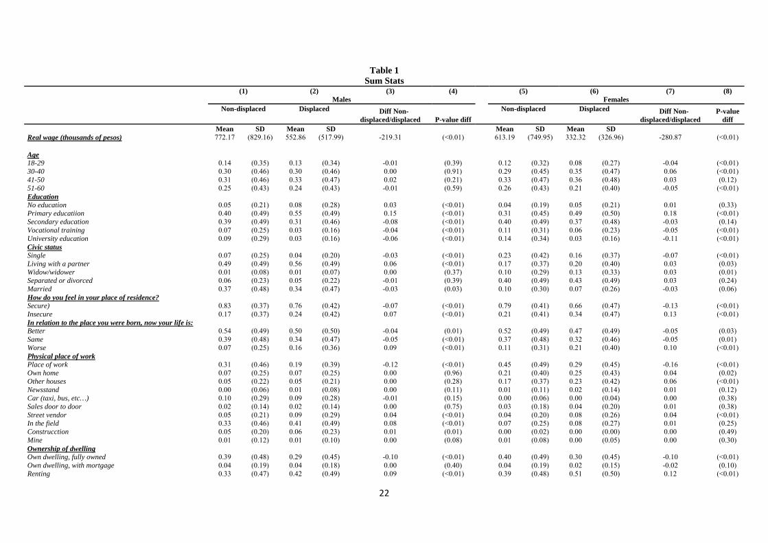
from the survey. Table 1 shows the average wage of selected workers, by displaced/non-
displaced status and gender.4 First, we observe that wages of women are lower than wages of
men, for both the group of displaced (552.86 vs. 332.32) and non-displaced (772.17 vs 613.19)
workers, with these differences being statistically significant at standard levels. Furthermore,
and comparing displaced and non-displaced workers, we observe that, for both men and women,
displaced workers have lower wages than those who are not displaced, with the differences
being statistically significant at the 99% level. In particular, for men, we observe that while
displaced male workers have an average wage of 552.86, non-displaced male workers have an
average wage of 772.17, a difference of 39.7% of the wage of displaced male workers. For
women, we observe that while displaced female workers have an average wage of 332.32, non-
displaced female workers have an average wage of 613.19, a difference of 84.5% of the wage
of displaced female workers. The differences in wages between the displaced and non-displaced
are very large, especially for women, which points toward the negative effects of forced
displacements on wages.
Thus, we observe that there are substantial differences in wages between displaced and non-
displaced workers, although these are raw differences and do not take into account other
differences in socio-demographic characteristics. For instance, it could be that displaced
workers come from poorer regions, where levels of education are comparatively lower, which
could explain part of the observed difference. Thus, in what follows, we attempt to net out the
effect of forced displacement from differences in socio-demographic characteristics. Other
3 Other options to the question are: 1) Difficulties to find a job or no resources to make living; 2) Risk of natural disaster (flood, avalanche…); 3) Natural disaster (flood, avalanche…); 5) Educational needs; 6) Because the respondent got married or formed a couple; 7) Health-related motives; 8) Improve of housing or location; 9) Better labor market opportunities or business opportunities; 10) Other reasons. 4 Given previous research showing gender discrimination in wages in Colombia (Seguino, 2000; Weichselbaumer and Winter-Ebner, 2005; Angel-Urdinola and Wodon, 2006), throughout the paper we will analyze men and women separately.
7
variables that may have some relationship to wages, and that are included in our analysis, are
age, education, civic status, physical place of work, ownership of dwelling, type of dwelling,
status of electricity rate, main material of exterior wall of the house, whether the dwelling has
running water, and the region of residence. Table 1 shows average values of all these variables,
where columns (1), (2), (5) and (6) show means and standard deviations of selected
characteristics for non-displaced men, displaced men, non-displaced women, and displaced
women, respectively. Columns (3) and (7) show the difference in average values between non-
displaced and displaced workers for men and women, respectively, where a negative coefficient
indicates that displaced workers present a lower value for the characteristic of reference.
Columns (4) and (8) show the p-value of the difference of average values, based on t-type tests
of the mean values, where a p-value lower than .05 indicates that the difference is statistically
significant at standard levels.
Age is measured in 10-year age groups. In the case of men, there are no significant
differences in the ages of displaced and non-displaced workers. However, in the case of women,
we observe that non-displaced workers are comparatively younger, as there is a higher
proportion of non-displaced workers in the age group of 18-29, with a lower proportion of them
in the age groups of 30-40 and 51-60. To the extent that age is an important determinant of
fertility, as mean age of women at childbirth in Colombia is around 21 years (Profamilia, 2014),
if individuals are displaced from more violent to less violent regions, those more violent regions
will experience a reduction in fertility, which may foster inequality and problems of violence.
Regarding education, we define levels of education as, 1) no education (illiteracy), 2) Primary
education, 3) Secondary education, 4) Vocational training, and 5) University education. We
observe that for both men and women, non-displaced workers present, in comparison to
displaced workers, a higher level of education as there is a higher proportion of workers with
secondary education, vocational training, and university education, while there is a lower
proportion of workers with primary education, and no education for men. These differences in
education may be one of the sources of the reported wage gap between displaced and non-
displaced workers. It may also indicate that displaced workers come originally from poorer
areas with lower levels of development, and thus the level education of displaced workers is
lower. These results are consistent with Ibañez and Querubin (2004), who find that the
enrollment rate in the group of displaced people is very low. For the civic status of workers,
five possible levels are considered: 1) single, 2) living with a partner, 3) widow, widowed, 4)
8
separated or divorced, and 5) married. We observe differences in civic status between displaced
and non-displaced workers, as displaced workers present a higher probability of living with a
partner, or being a widow or widower, and a lower probability of being single or married.
In the survey, there are two questions that allow us to analyze how workers feel about their
degree of security, and their wellbeing. Regarding the degree of perceived security, we use the
information from the response to the question “How do you feel in your place of residence?”,
with two possible responses: 1) secure; 2) insecure. We find differences between displaced and
non-displaced workers, as non-displaced workers report higher levels of perceived security in
comparison with displaced workers, for both men and women. As for the wellbeing of workers,
we use the information from the response to the question “In relation to the place you were
born, now your life is”, with three possible responses: 1) better, 2) the same, and 3) worse.
Comparing the two groups, we observe that displaced workers are less satisfied with their
current life, as they have comparatively greater probabilities of reporting worse living
conditions than non-displaced workers.
The variable for the physical place of work refers to whether workers develop their tasks in
the company’s offices/facilities, the respondent’s home, or other places. Here, we must
highlight that, while non-displaced workers are more likely to work at the firm’s facilities,
displaced workers are more likely to work as street vendors. This is consistent with Ibañez and
Querubin (2004), who find that there is a higher degree of informality regarding work for the
group of displaced people, as we may consider street vendors as highly informal.
Another characteristic that may be related to wages is that of housing. In the survey, we have
information on the ownership of the dwelling (e.g., own dwelling fully owned, own dwelling
with mortgage, renting, usufruct, and occupied without ownership) and the type of dwelling
(house, apartment, or room). We observe differences between displaced and non-displaced
workers for these characteristics, as non-displaced workers are less likely to have a house fully
owned, and more likely to have a rented house, and they are also more likely to live in rooms
and be less likely to live in apartments, in comparison with non-displaced workers. One
important question in Colombia is that of the electricity rate. Depending on the economic status
of the household, households pay different rates for the services. High-income households pay
a “high” rate, while other households with fewer resources pay a “medium” or “low” rate, as
the price of the service is partially subsidized. We observe that displaced workers are more
9
likely to pay a “high” rate. Furthermore, we also contemplate possible differences in the
materials of exterior walls of the dwelling, as this factor has been reported to be important in
Colombia. Several possibilities are considered in the survey (bricks, adobe, wood), although
we do not find significant differences between the two groups of workers.
Finally, we consider differences in the region of residence, as the level of violence may differ
depending on the specific area. For instance, Angrist and Kugler (2008) find that the variation
in the prices of natural resources affects the level of violence in the region. Thus, the number
or origin of displaced workers differs depending on the region of residence, and thus we
consider the nine regions described in the survey: Atlántida, Oriental, Central, Pacifica, Bogotá,
Antioquia, Valle del Cauca, San Andrés and Orinoquia-Amazonía.
4. PROPENSITY SCORE MATCHING: RESULTS
The PSM approach has been traditionally used to evaluate employment and education programs
(Lalonde 1986; Rosembaun and Rubin, 1983; Fraker and Maynard 1987; Heckman, Ichimura
and Todd, 1998; Lechner, 1999; Dehejia and Wahba, 2002; Jalan and Ravallion, 2003; Smitch
and Tood, 2005), especially suitable in cases when an experimental design is infeasible, which
allows the matching of individuals in one treatment group to others who did not participate, but
have comparable characteristics.5 The innovation of PSM, compared to other matching
methods, is that it develops a single (propensity) score that encapsulates multiple
characteristics, rather than requiring a one-to-one match of each characteristic, simplifying
matching by reducing dimensionality. The interest in PSM accelerated after Heckman et al.
(1998a,b) assessed the validity of using propensity matching to characterize selection bias using
experimental data. PSM employs a predicted probability of group membership (treatment vs.
control group), based on observed predictors usually obtained from a logistic regression to
create a counterfactual group. Once the treated and control groups have been defined, and the
score has been calculated, observations in the two groups are matched and compared in order
to obtain the effect of the treatment on the treated.
In the current context, we define as control group those who have not been displaced, while
our treated group includes all workers forcibly displaced through violence. In the PSM
5 See Caliendo and Kopeinig (2008) for a review of the PSM technique, and guidance for the implementation of the method.
10
approach, the main characteristic of the treatment under evaluation is its exogeneity, in the
sense that the treatment is not controllable by the individuals. Then, those who are treated may
choose to behave in different ways, depending on their preferences and/or characteristics,
among other factors. Here, we make the assumption that the level of violence in the residence
of origin is exogenous and not controllable by the individual who moved, and thus, those who
moved were treated by “violence” as it reached a level that was not tolerable.
The PSM matches and calculates the propensity to participate or not, in a treatment based on
the observable characteristics of individuals. If, in the calculation of the score, the required
hypotheses are fulfilled, it compares the pre- and post- results independent of the participation,
in the sense that it creates an unbiased estimator (Average effect of Treatment on the Treated –
ATT), imposing that the participation in the treatment is the only differential factor between the
treated and the control group.6 This method comprises several steps. We first specify and
estimate a binomial probit model of the probability of belonging to the displaced sample; and
we obtain the Propensity Score (PS). Second, we impose the common support condition; that
is, we restrict the non-displaced sample to observations whose estimated PS lies within the
ranges of estimated PS of the displaced. Third, we pair each individual from the displaced
sample with another individual from the non-displaced sample. Fourth, we compute the ATT.7
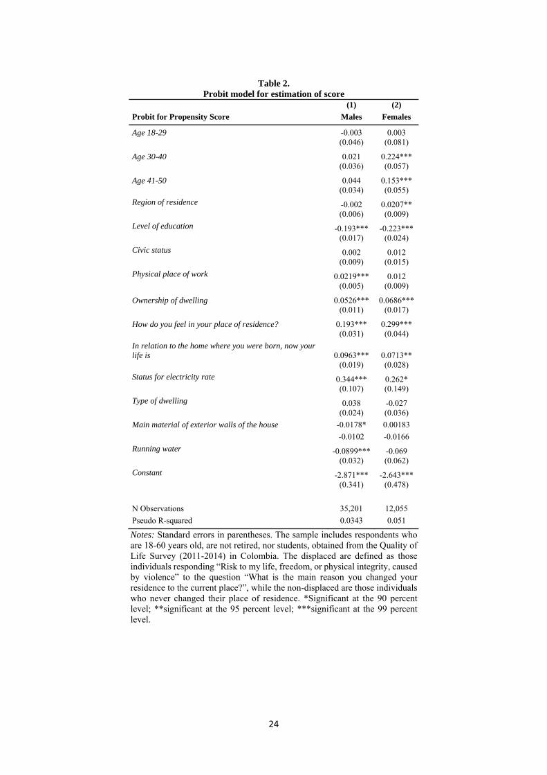
The PS is defined as the probability of being displaced, conditional on the common observed
covariates (p(Xi)=Pr(i ϵ displaced| X=x)). Table 2 shows the results from the probit model of
the likelihood of belonging to the displaced sample, for men and women separately. We run a
probit regression of the binary indicator, taking value “1” for observations in the displaced
sample, and “0” for observations in the non-displaced sample, over the set of common variables.
We consider the demographic and personal characteristics described in the previous Section. In
the estimation of the PS, the balancing property is fulfilled (the mean propensity score is the
6 Three hypotheses (Rosenbaum y Rubin 1983; Becker and Ichino, 2002) must be fulfilled to match individuals: 1) An equilibrium must exist in the group of selected covariates, as individuals with the same Propensity Score must have the same distribution of characteristics, independently of whether they pertain to the treated group (those who experienced a forcible displacement) or not; 2) Conditional Independence Assumption (CIA, Rubin, 1997), which means that the dependent variable (wages) conditioned on covariates for the group of the treated has the same distribution as the dependent variable (wages) conditioned on covariates for the group of the treated; 3) Stable Unit Treatment Value Assumption (SUTVA, Angrits, Imbens and Rubin, 1996), which indicates that the observed result for unit I under treatment t is the same, independently of what is the assignment mechanism of the treatment, and of what treatment the rest of the units receive.
7 The PSM has been done using the “psmatch2” command in STATA.

11
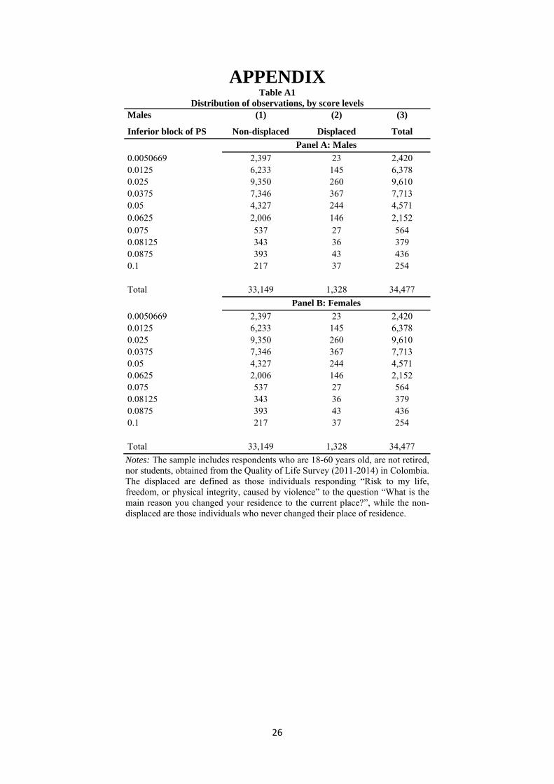
same for treated and untreated individuals in each block).8 Once the probit model for the
probability of being displaced has been estimated, we calculate the PS (see Table A1 in the
Appendix for a description of the distribution of the Propensity Score) and impose the common
support restriction to obtain the ATT, in the sense that we adjust the group of non-displaced
workers whose PS is in the range of the Propensity Score of the group of displaced workers.9
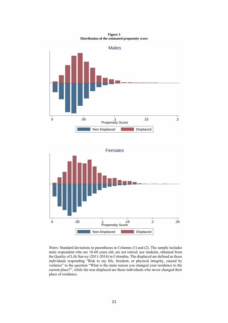
Figure 3 shows the PS histograms for both datasets, and for men and women, respectively,
showing a high degree of overlap between the two distributions, indicating that the common
support assumption is satisfied. Regarding the factors that affect the probability of being
displaced, we find that greater age, a lower level of education, the ownership of the dwelling
(rent is related to a higher probability of being displaced, vs. ownership), if the individuals feel
insecure in their place of residence, and higher rates for electricity, are all factors related to a
higher probability of being a displaced worker.
Once the PS has been calculated for workers in the two groups, we match them based on the
PS and calculate the effect of treatment on our variable of interest (wages). For matching of the
observations, we use several methods: nearest neighbor, radius, stratification, and kernel
matching (see Caliendo and Kopeinig (2008) for a description of each algorithm). For the
nearest neighbor matching, each treated observation is matched with an untreated observation
with the closest PS. With this method, it could be the case that several treated observations are
matched to the same untreated observations, and in that case the ATT is calculated as an average
difference (Becker and Ichino, 2002). But nearest neighbor matching faces the risk of bad
matches, if the closest neighbour is far away. This can be avoided by imposing a tolerance level
on the maximum propensity score distance (caliper). Dehejia and Wahba (2002) suggest a
variant of caliper matching, called radius matching. The basic idea of this variant is to use not
only the nearest neighbour within each caliper, but all of the comparison members within the
8 In the literature of the evaluation of public policies/programs, researchers must face the dimensionality problem, which is the lack of common support between treated and untreated groups with cells containing treated observations and/or untreated observations only, and it arises when the number of covariates is large, or many of the covariates have many values, or are continuous. In this framework, the “Balancing Property” establishes that the mean propensity score must not be different for treated and untreated individuals in each cell, and if this property is not fulfilled, a less parsimonious specification of the propensity score is needed. The fulfilling of this property prevents us from introducing all the categorical variables as vectors of dummy variables, and some are included as continuous covariates.
9 In the process, 10 and 8 blocks are created for men and women, respectively. Hypothesis 1 (Equilibrium condition) is fulfilled as in each interval of the PS its mean value does not differ between the treated and untreated observations; that is, the average PS is the same for displaced and non-displaced workers in each block.
12
caliper. A benefit of this approach is that it uses only as many comparison units as are available
within the caliper and therefore allows for usage of extra (fewer) units when good matches are
(not) available. Hence, it reduces the risk of bad matches
The idea of stratification matching is to partition the common support of the propensity score
into a set of intervals (strata) and to calculate the impact within each interval by taking the mean
difference in outcomes between treated and control observations. This method is also known as
interval matching, blocking, and sub-classification (Rosenbaum and Rubin, 1983). Cochrane
and Chambers (1965) show that five subclasses are often enough to remove 95% of the bias
associated with a single covariate. Since, as Imbens (2004) notes, all bias under
‘unconfoundedness’ is associated with the propensity score, suggesting that under normality
the use of five strata removes most of the bias associated with all covariates.
The matching algorithms described so far have in common that only a few observations from
the comparison group are used to construct the counterfactual outcome of a treated individual.
Kernel matching is a non-parametric matching estimator that uses weighted averages of all
individuals in the control group to construct the counterfactual outcome. Thus, one major
advantage of this approach is the lower variance that is achieved, because more information is
used. A drawback of this method is that, potentially, observations are used that are bad matches.
Hence, the proper imposition of the common support condition is of major importance for this
procedure.
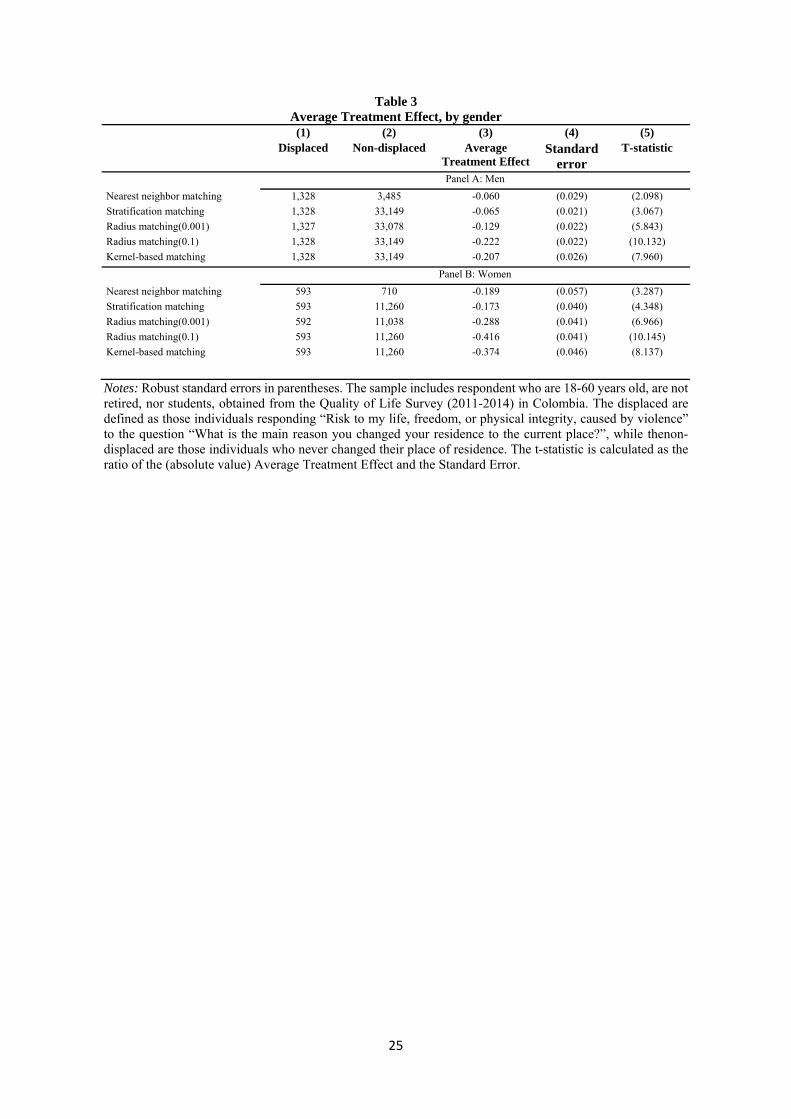
Panels A and B of Table 3 show the results of estimating the ATT based on the nearest
neigbour, stratification, radius (0.001), radius (0.01), and kernel matching, for men and women,
respectively. Wages have been transformed to log form so that the effects can be interpreted as
changes in percentage points. We show the ATT, the standard error of the ATT, and the t-ratio
calculated as the ratio between the ATT (in absolute values) and its standard error. T-ratios
higher than 1.96 indicate that the effect is statistically significant at the 9% confidence level.
We observe that, in all cases, the t-ratios are higher than 1.96, indicating, independently of the
algorithm matching used to calculate the ATT, that we obtain a statistically significant effect.
In the case of men, the ATT calculated using the nearest neigbour, stratification, radius (0.001),
radius (0.01), and kernel matching are -0.06, -0.065, -0.129, -0.222 and -0.207, respectively. In
the case of women, the corresponding ATT are -0.189, -0.173, -0.288, -0.416, and -0.374,
respectively. Thus, we find that forced displacement decreases by between 6% and 22% the
13
wages of males, and by between 17% and 37% the wages of females, compared to their non-
displaced counterparts.
5. CONCLUSIONS
In this paper, we analyze how forcible displacements caused by violent conflict affect the wages
of workers in Colombia. This analysis is important, as the phenomenon is far from disappearing,
and has become a global concern. Using the data offered by the Quality of Life Survey (QLS)
in Colombia for the years 2011 to 2014, we compare the wages of those who were forced to
abandon their place of residence, through violence, with those who were not forced to do so,
and we find that forcible displacement decreases by between 6% and 22% the wages of males,
and by between 17% and 37% the wages of females, relative to their non-displaced
counterparts.
Our results are consistent with prior results showing that forced displacements due to
violence negatively affect labor market outcomes; when combined with the cases where one
member of the couple dies in a violent conflict, the economic conditions lead to lives of
isolation and marginalization. Thus, we have identified a source of income inequality in a
country already characterized by a high level of inequality, and thus public policies focused on
mitigating the negative impact of forced displacements, via subsidies or reduction in prices of
public services, may help to alleviate such conditions. Furthermore, this negative effect has a
greater impact on women, who are an important factor in the educational and childcare systems.
Finally, forced displacements contribute negatively to the development of the country, and pose
unique challenges for crafting state policy to effectively mitigate the impacts of displacement,
and an analysis of the economic consequences of this phenomenon may help to guide public
policies of alleviation.
Our results will encourage future research on this topic, at the theoretical and empirical
levels, seeking, especially, to find answers to the question of why women in particular are more
affected by this negative shock. One extension to the analysis would be to analyze why the
subsidies given by the Colombian government are insufficient in solving this problem.
Subsidies and psychological support must form a basis for displaced individuals, as they are
exiled from their regions of origin, with few, if any, resources, in conditions of fear and anguish.
Colombia has a well- developed judicial framework, but its serious challenge is to make it work.
14
Another extension would be the analysis of labor-force participation decisions. Here we have
focused on wages, assuming that labor-force participation decisions are exogenous to the
treatment. However, it is necessary to analyze the extent to which the displaced behave
differently behavior in the labor market, which may also help to explain income inequality.
One of the limitations of our analysis is that the sample of displaced people is relatively
small, given the difficulties of finding individuals willing to answer the questions used in the
survey. As the survey is implemented in the future, the sample size will increase, and more
topics related to forcible displacement will come to the fore.
REFERENCES
Abadie, A., & Gardeazabal, J. (2003). The economic costs of conflict: A case study of the Basque Country. American Economic Review, 93, 113-132.
Angel-Urdinola, D. F., & Wodon, Q. (2006). The gender wage gap and poverty in Colombia. Labour, 20, 721-739.
Angrist, J. D., Imbens, G. W., & Rubin, D. B. (1996). Identification of causal effects using instrumental variables. Journal of the American Statistical Association, 91, 444-455.
Angrist, J. D., & Kugler, A. D. (2008). Rural windfall or a new resource curse? Coca, income, and civil conflict in Colombia. The Review of Economics and Statistics, 90, 191-215.
Attanasio, O., Goldberg, P. K., & Pavcnik, N. (2004). Trade reforms and wage inequality in Colombia. Journal of Development Economics, 74, 331-366.
Becker, S. O., & Ichino, A. (2002). Estimation of average treatment effects based on propensity scores. The Stata Journal, 2, 358-377.
Bell, L. A. (1997). The impact of minimum wages in Mexico and Colombia. Journal of Labor Economics, 15, S102-S135.
Birchenall, J. A. (2001). Income distribution, human capital and economic growth in Colombia. Journal of Development Economics, 66, 271-287.
Blattman, C., & Miguel, E. (2009). Civil War. NBER Working Paper No. 14801.National Bureau of Economic Research.
Blattman, C., & Miguel, E. (2010). Civil war. Journal of Economic Literature, 48, 3-57.
Bonikowska, A., & Morissette, R. (2012). Earnings losses of displaced workers with stable labour market attachment: recent evidence from Canada. Statistics Canada.
Bourguignon, F., Nuñez, J., & Sanchez, F. (2003). A structural model of crime and inequality in Colombia. Journal of the European Economic Association, 1, 440-449.
15
Caliendo, M., & Kopeinig, S. (2008). Some practical guidance for the implementation of propensity score matching. Journal of Economic Surveys, 22, 31-72.
Castilla, E. J. (2005). Social networks and employee performance in a call center1. American Journal of Sociology, 110, 1243-1283.
Cochran, W. G., & Chambers, S. P. (1965). The planning of observational studies of human populations. Journal of the Royal Statistical Society Series A, 128, 234-266.
Collier, P., Hoeffler, A., & Pattillo, C. A. (1999). Flight capital as a portfolio choice. World Bank Working Paper 2066, Washington, DC.
Collier, P., Hoeffler, A., & Pattillo, C. (2004). Africa's exodus: Capital flight and the brain drain as portfolio decisions. Journal of African Economies, 13, ii15-ii54.
Couch, K. A., & Placzek, D. W. (2010). Earnings losses of displaced workers revisited. The American Economic Review, 100, 572-589.
Dehejia, R. H., & Wahba, S. (1999). Causal effects in nonexperimental studies: Reevaluating the evaluation of training programs. Journal of the American Statistical Association, 94, 1053-1062.
Dehejia, R. H., & Wahba, S. (2002). Propensity score-matching methods for nonexperimental causal studies. Review of Economics and Statistics, 84, 151-161.
Deininger, K. W. (2003). Land policies for growth and poverty reduction. World Bank Publications.
Deininger, K. (2003). Causes and consequences of civil strife: micro-level evidence from Uganda. Oxford Economic Papers, 55, 579-606.
Dube, O., & Vargas, J. F. (2013). Commodity price shocks and civil conflict: Evidence from Colombia. The Review of Economic Studies, 80, 1384-1421.
Eliason, M., & Storrie, D. (2006). Lasting or latent scars? Swedish evidence on the long-term effects of job displacement. Journal of Labor Economics, 24, 831-856.
Engel, S., & Ibáñez, A. M. (2007). Displacement Due to Violence in Colombia: A Household�Level Analysis. Economic Development and Cultural Change, 55, 335-365.
Fields, G. S. (1979). Place-to-place migration: Some new evidence. The Review of Economics and Statistics, 61, 21-32.
Fields, G. S., & Schultz, T. P. (1980). Regional inequality and other sources of income variation in Colombia. Economic Development and Cultural Change, 28, 447-467.
Fraker, T., & Maynard, R. (1987). The adequacy of comparison group designs for evaluations of employment-related programs. Journal of Human Resources, 22, 194-227.
Garay, L. J. (2008). Proceso nacional de verificación de los derechos de la población desplazada. First Report to the Colombian Constitutional Court.
16
Heckman, J. J. (1979). Sample selection bias as a specification error. Econometrica: Journal of the Econometric Society, 47, 153-161.
Heckman, J., Ichimura, H., Smith, J., & Todd, P. (1998a). Characterizing selection bias using experimental data (No. w6699). National Bureau of Economic Research.
Heckman, J. J., Ichimura, H., & Todd, P. (1998b). Matching as an econometric evaluation estimator. The Review of Economic Studies, 65, 261-294.
Hijzen, A., Upward, R., & Wright, P. W. (2010). The income losses of displaced workers. Journal of Human Resources, 45, 243-269.
Ibañez, A.M. (2009). “Forced displacement in Colombia: Magnitude and causes.” The Economics of Peace and Security, 4, 48-54.
Ibáñez, A. M., & Moya, A. (2006). The Impact of Intra-State Conflict on Economic Welfare and Consumption Smoothing: Empirical Evidence for the Displaced Population in Colombia. Available at SSRN 1392415.
Ibáñez, A. M., & Moya, A. (2007). ¿Cómo deteriora el desplazamiento forzado el bienestar de los hogares desplazados? Análisis y determinantes del bienestar en los municipios de recepción (No. 012865). FEDESARROLLO.
Ibáñez, A. M., & Querubín, P. (2004). Acceso a tierras y desplazamiento forzado en Colombia. Documento Cede, 23, 1-114.
Ibáñez, A. M., & Velásquez, A. (2008). El impacto del desplazamiento forzoso en Colombia: condiciones socioeconómicas de la población desplazada, vinculación a los mercados laborales y políticas públicas. CEPAL.
Imbens, G. W. (2004). Nonparametric estimation of average treatment effects under exogeneity: A review. Review of Economics and Statistics, 86, 4-29.
Jacobson, L. S., LaLonde, R. J., & Sullivan, D. G. (1993). Earnings losses of displaced workers. American Economic Review, 83, 685-709.
Jalan, J., & Ravallion, M. (2003). Estimating the benefit incidence of an antipoverty program by propensity-score matching. Journal of Business & Economic Statistics, 21, 19-30.
Knight, M., Loayza, N., & Villanueva, D. (1996). The peace dividend: military spending cuts and economic growth. World Bank Policy Research Working Paper, (1577).
Kondylis, F. (2008). Agricultural outputs and conflict displacement: Evidence from a policy intervention in Rwanda. Economic Development and Cultural Change, 57, 31-66.
Kondylis, F. (2010). Conflict displacement and labor market outcomes in post-war Bosnia and Herzegovina. Journal of Development Economics, 93, 235-248.
LaLonde, R. J. (1986). Evaluating the econometric evaluations of training programs with experimental data. American Economic Review, 76, 604-620.

17
Lechner, M. (1999). An evaluation of public-sector-sponsored continuous vocational training programs in East Germany. University of St. Gallen Working Paper, (9901).
Meertens, D., & Stoller, R. (2001). Facing destruction, rebuilding life: Gender and the internally displaced in Colombia. Latin American Perspectives, 28, 132-148.
Mohan, R., & Sabot, R. (1988). Educations expansion and the inequality of pay: Colombia 1973-78. Oxford Bulletin of Economics and Statistics, 50, 175-182.
Mouw, T. (2003). Social capital and finding a job: Do contacts matter? American Sociological Review, 68, 868-898.
Profamilia (2014). Encuesta Nacional de Demografía y Salud. 2010
Rosenbaum, P. R., & Rubin, D. B. (1983). The central role of the propensity score in observational studies for causal effects. Biometrika, 70, 41-55.
Rubin, D. B. (1997). Estimating causal effects from large data sets using propensity scores. Annals of Internal Medicine, 127, 757-763.
Sanders, J. M., & Nee, V. (1996). Immigrant self-employment: The family as social capital and the value of human capital. American Sociological Review, 61, 231-249.
Schmieder, J. F., von Wachter, T., & Bender, S. (2010). The long-term impact of job displacement in Germany during the 1982 recession on earnings, income, and employment (No. 2010, 1). IAB discussion paper.
Seguino, S. (2000). Gender inequality and economic growth: A cross-country analysis. World Development, 28, 1211-1230.
Seim, D. (2012). Job displacement and labor market outcomes by skill level (No. wp2012-4). Bank of Estonia.
Smith, J. A., & Todd, P. E. (2005). Does matching overcome LaLonde's critique of nonexperimental estimators? Journal of Econometrics, 125, 305-353.
Weichselbaumer, D., & Winter-Ebmer, R. (2005). A Meta-Analysis of the International Gender Wage Gap. Journal of Economic Surveys, 19, 479-511.
18
LINKS TO STATISTICAL SOURCES
http://www.dane.gov.co/index.php/esp/estadisticas-sociales/pobreza/87-sociales/calidad-de-vida/5405-pobreza-monetaria-y-multidimensional-2013 (DANE, 2013)
https://www.cia.gov/library/publications/the-world factbook/rankorder/2172rank.html (The World Factbook, 2014).
http://www.internal-displacement.org/ (IDMC).
http://www.internal-displacement.org/global-figures (IDMC).
http://rni.unidadvictimas.gov.co/ (UARIV).
http://www.codhes.org/ (CODHES).
https://www.icrc.org/es/homepage (CICR).
http://www.dane.gov.co/index.php/estadisticas-sociales/calidad-de-vida-ecv (QLS)
19
Figure 1 Forced displacements in Colombia, 1985-2013
Notes: Author’s calculation. CODHES is the acronym for “Consultoria para los derechos humanos y el desplazamiento”, a prívate institution aimed at collecting statistics regarding human rights, including statistics for forced displacements. UARIV is the acronym for “Unidad para la atención y reparación integral a las victimas”.
119.000
308.000
317.375
412.553
380.863
280.041
224887
22.783
198.878
481.905
677.131
395.250
168.112
213.896
0
100.000
200.000
300.000
400.000
500.000
600.000
700.000
800.000
1985
1986
1987
1988
1989
1990
1991
1992
1993
1994
1995
1996
1997
1998
1999
2000
2001
2002
2003
2004
2005
2006
2007
2008
2009
2010
2011
2012
2013
Nunmber of displaced peo
ple
Años
CODHES UARIV
20
Figure 2 Global Internal displacements, 2013
Notes: Authors calculations using the data from the “Observatorio de Desplazamiento Interno (IDMC)”.
17
150
160
242
212,4
218
280
307
316
412
526
543,4
631
640,9
746,7
935
953,7
1100
2100
2426,7
2963,7
3300
5702,1
6500
Countries
Syria Colombia Nigeria DRC Sudan Iraq
Somalia Turquia CAR Pakistan Myanmar Afghanistan
Azerbaijan India Kenia Ethiopia Yemen Bangladesh
Mali Cyprus Guatemala Mexico Peru Honduras
21
Figure 3 Distribution of the estimated propensity score
Notes: Standard deviations in parentheses in Columns (1) and (2). The sample includes male respondent who are 18-60 years old, are not retired, nor students, obtained from the Quality of Life Survey (2011-2014) in Colombia. The displaced are defined as those individuals responding “Risk to my life, freedom, or physical integrity, caused by violence” to the question “What is the main reason you changed your residence to the current place?”, while the non-displaced are those individuals who never changed their place of residence.
0 .05 .1 .15 .2Propensity Score
Non-Displaced Displaced
Males
0 .05 .1 .15 .2 .25Propensity Score
Non-Displaced Displaced
Females
22
Table 1 Sum Stats
(1) (2) (3) (4) (5) (6) (7) (8) Males Females Non-displaced Displaced Diff Non-
displaced/displaced P-value diff
Non-displaced Displaced Diff Non-displaced/displaced
P-value diff
Mean SD Mean SD Mean SD Mean SD Real wage (thousands of pesos) 772.17 (829.16) 552.86 (517.99) -219.31 (<0.01) 613.19 (749.95) 332.32 (326.96) -280.87 (<0.01) Age 18-29 0.14 (0.35) 0.13 (0.34) -0.01 (0.39) 0.12 (0.32) 0.08 (0.27) -0.04 (<0.01) 30-40 0.30 (0.46) 0.30 (0.46) 0.00 (0.91) 0.29 (0.45) 0.35 (0.47) 0.06 (<0.01) 41-50 0.31 (0.46) 0.33 (0.47) 0.02 (0.21) 0.33 (0.47) 0.36 (0.48) 0.03 (0.12) 51-60 0.25 (0.43) 0.24 (0.43) -0.01 (0.59) 0.26 (0.43) 0.21 (0.40) -0.05 (<0.01) Education No education 0.05 (0.21) 0.08 (0.28) 0.03 (<0.01) 0.04 (0.19) 0.05 (0.21) 0.01 (0.33) Primary educatiion 0.40 (0.49) 0.55 (0.49) 0.15 (<0.01) 0.31 (0.45) 0.49 (0.50) 0.18 (<0.01) Secondary education 0.39 (0.49) 0.31 (0.46) -0.08 (<0.01) 0.40 (0.49) 0.37 (0.48) -0.03 (0.14) Vocational training 0.07 (0.25) 0.03 (0.16) -0.04 (<0.01) 0.11 (0.31) 0.06 (0.23) -0.05 (<0.01) University education 0.09 (0.29) 0.03 (0.16) -0.06 (<0.01) 0.14 (0.34) 0.03 (0.16) -0.11 (<0.01) Civic status Single 0.07 (0.25) 0.04 (0.20) -0.03 (<0.01) 0.23 (0.42) 0.16 (0.37) -0.07 (<0.01) Living with a partner 0.49 (0.49) 0.56 (0.49) 0.06 (<0.01) 0.17 (0.37) 0.20 (0.40) 0.03 (0.03) Widow/widower 0.01 (0.08) 0.01 (0.07) 0.00 (0.37) 0.10 (0.29) 0.13 (0.33) 0.03 (0.01) Separated or divorced 0.06 (0.23) 0.05 (0.22) -0.01 (0.39) 0.40 (0.49) 0.43 (0.49) 0.03 (0.24) Married 0.37 (0.48) 0.34 (0.47) -0.03 (0.03) 0.10 (0.30) 0.07 (0.26) -0.03 (0.06) How do you feel in your place of residence? Secure) 0.83 (0.37) 0.76 (0.42) -0.07 (<0.01) 0.79 (0.41) 0.66 (0.47) -0.13 (<0.01) Insecure 0.17 (0.37) 0.24 (0.42) 0.07 (<0.01) 0.21 (0.41) 0.34 (0.47) 0.13 (<0.01) In relation to the place you were born, now your life is: Better 0.54 (0.49) 0.50 (0.50) -0.04 (0.01) 0.52 (0.49) 0.47 (0.49) -0.05 (0.03) Same 0.39 (0.48) 0.34 (0.47) -0.05 (<0.01) 0.37 (0.48) 0.32 (0.46) -0.05 (0.01) Worse 0.07 (0.25) 0.16 (0.36) 0.09 (<0.01) 0.11 (0.31) 0.21 (0.40) 0.10 (<0.01) Physical place of work Place of work 0.31 (0.46) 0.19 (0.39) -0.12 (<0.01) 0.45 (0.49) 0.29 (0.45) -0.16 (<0.01) Own home 0.07 (0.25) 0.07 (0.25) 0.00 (0.96) 0.21 (0.40) 0.25 (0.43) 0.04 (0.02) Other houses 0.05 (0.22) 0.05 (0.21) 0.00 (0.28) 0.17 (0.37) 0.23 (0.42) 0.06 (<0.01) Newsstand 0.00 (0.06) 0.01 (0.08) 0.00 (0.11) 0.01 (0.11) 0.02 (0.14) 0.01 (0.12) Car (taxi, bus, etc…) 0.10 (0.29) 0.09 (0.28) -0.01 (0.15) 0.00 (0.06) 0.00 (0.04) 0.00 (0.38) Sales door to door 0.02 (0.14) 0.02 (0.14) 0.00 (0.75) 0.03 (0.18) 0.04 (0.20) 0.01 (0.38) Street vendor 0.05 (0.21) 0.09 (0.29) 0.04 (<0.01) 0.04 (0.20) 0.08 (0.26) 0.04 (<0.01) In the field 0.33 (0.46) 0.41 (0.49) 0.08 (<0.01) 0.07 (0.25) 0.08 (0.27) 0.01 (0.25) Construcction 0.05 (0.20) 0.06 (0.23) 0.01 (0.01) 0.00 (0.02) 0.00 (0.00) 0.00 (0.49) Mine 0.01 (0.12) 0.01 (0.10) 0.00 (0.08) 0.01 (0.08) 0.00 (0.05) 0.00 (0.30) Ownership of dwelling Own dwelling, fully owned 0.39 (0.48) 0.29 (0.45) -0.10 (<0.01) 0.40 (0.49) 0.30 (0.45) -0.10 (<0.01) Own dwelling, with mortgage 0.04 (0.19) 0.04 (0.18) 0.00 (0.40) 0.04 (0.19) 0.02 (0.15) -0.02 (0.10) Renting 0.33 (0.47) 0.42 (0.49) 0.09 (<0.01) 0.39 (0.48) 0.51 (0.50) 0.12 (<0.01)

23
Usufruct 0.22 (0.41) 0.23 (0.42) 0.01 (0.18) 0.15 (0.35) 0.15 (0.35) 0.00 (0.68) Occupied without ownership 0.02 (0.15) 0.02 (0.14) 0.00 (0.46) 0.02 (0.14) 0.02 (0.14) 0.00 (0.95) Type of dwelling House 0.72 (0.45) 0.73 (0.44) 0.01 (0.23) 0.64 (0.48) 0.66 (0.47) 0.02 (0.31) Apartment 0.24 (0.43) 0.22 (0.41) -0.02 (0.02) 0.32 (0.46) 0.31 (0.46) -0.01 (0.54) Room 0.04 (0.18) 0.05 (0.21) 0.01 (0.01) 0.04 (0.21) 0.03 (0.19) -0.01 (0.33) Status for electricity rate High 0.96 (0.18) 0.99 (0.28) 0.02 (<0.01) 0.79 (0.40) 0.90 (0.29) 0.11 (<0.01) Medium 0.03 (0.15) 0.01 (0.28) -0.02 (<0.01) 0.20 (0.39) 0.09 (0.29) -0.11 (<0.01) Low 0.01 (0.10) 0.00 (0.02) -0.01 (<0.01) 0.01 (0.10) 0.00 (0.00) -0.01 (0.01) Main material of exterior walls of the house Bricks 0.82 (0.38) 0.81 (0.39) -0.01 (0.23) 0.85 (0.35) 0.82 (0.38) -0.03 (0.01) Adobe 0.04 (0.18) 0.05 (0.21) 0.01 (0.01) 0.03 (0.17) 0.04 (0.20) 0.01 (0.06) Covered canes and clay 0.04 (0.19) 0.03 (0.18) -0.01 (0.23) 0.03 (0.16) 0.02 (0.13) -0.01 (0.17) Uncovered canes and clay 0.02 (0.16) 0.02 (0.13) 0.00 (0.05) 0.01 (0.12) 0.01 (0.10) 0.00 (0.56) Wood 0.06 (0.24) 0.07 (0.26) 0.01 (0.08) 0.06 (0.23) 0.10 (0.29) 0.04 (0.00) Prefabricated material 0.00 (0.06) 0.01 (0.08) 0.00 (0.15) 0.01 (0.07) 0.00 (0.04) 0.00 (0.25) Cane, rush matting, other vegetable 0.01 (0.07) 0.01 (0.09) 0.00 (0.17) 0.01 (0.07) 0.00 (0.05) 0.00 (0.49) Zinc, coal, other waste 0.00 (0.05) 0.00 (0.03) -0.01 (0.28) 0.00 (0.04) 0.00 (0.04) 0.00 (0.86) Running water Yes 0.79 (0.40) 0.78 (0.41) -0.01 (0.85) 0.87 (0.33) 0.86 (0.34) -0.01 (0.76) No 0.21 (0.40) 0.22 (0.41) 0.01 (0.85) 0.13 (0.33) 0.14 (0.34) 0.01 (0.76) Region Atlántica 0.17 (0.37) 0.16 (0.39) -0.01 (0.57) 0.15 (0.35) 0.13 (0.33) -0.02 (0.20) Oriental 0.15 (0.35) 0.12 (0.25) -3.00 (<0.01) 0.14 (0.34) 0.08 (0.28) -0.06 (<0.01) Central 0.13 (0.33) 0.16 (0.21) 0.03 (<0.01) 0.11 (0.31) 0.12 (0.32) 0.01 (0.60) Pacífica (sin Valle) 0.16 (0.36) 0.23 (0.09) 0.07 (<0.01) 0.19 (0.39) 0.28 (0.40) 0.09 (<0.01) Bogotá 0.08 (0.26) 0.04 (0.27) -0.04 (<0.01) 0.10 (0.30) 0.04 (0.19) -0.06 (<0.01) Antioquía 0.11 (0.31) 0.14 (0.14) 0.03 (<0.01) 0.10 (0.30) 0.16 (0.36) 0.06 (<0.01) Valle del Cauca 0.13 (0.34) 0.12 (0.29) -0.01 (0.36) 0.13 (0.33) 0.12 (0.32) -0.01 (0.50) San Andrés 0.04 (0.18) 0.00 (0.50) -0.04 (<0.01) 0.04 (0.18) 0.01 (0.08) -0.03 (<0.01) Orinoquía - Amazonía 0.03 (0.16) 0.02 (0.24) -0.01 (<0.01) 0.04 (0.18) 0.06 (0.22) 0.02 (0.02)
N observations 33,873 1,328 11,462 593
Notes: Standard deviations in parentheses in Columns (1) and (2). The sample includes male respondent who are 18-60 years old, are not retired, nor students, obtained from the Quality of Life Survey (2011-2014) in Colombia. The displaced are defined as those individuals responding “Risk to my life, freedom, or physical integrity, caused by violence” to the question “What is the main reason you changed your residence to the current place?”, while the non-displaced are those individuals who never changed their place of residence. The difference is defined as the average values of the displaced minus the average values of the non-displaced. The p-value of the difference is computed as the probability of accepting the hypothesis of the equality of average values between the 2 groups, based on a t-type test.
24
Table 2. Probit model for estimation of score
(1) (2)
Probit for Propensity Score Males Females
Age 18-29 -0.003 0.003
(0.046) (0.081)
Age 30-40 0.021 0.224***
(0.036) (0.057)
Age 41-50 0.044 0.153*** (0.034) (0.055)
Region of residence -0.002 0.0207** (0.006) (0.009)
Level of education -0.193*** -0.223*** (0.017) (0.024)
Civic status 0.002 0.012 (0.009) (0.015)
Physical place of work 0.0219*** 0.012 (0.005) (0.009)
Ownership of dwelling 0.0526*** 0.0686*** (0.011) (0.017)
How do you feel in your place of residence? 0.193*** 0.299*** (0.031) (0.044)
In relation to the home where you were born, now your life is 0.0963*** 0.0713** (0.019) (0.028)
Status for electricity rate 0.344*** 0.262* (0.107) (0.149)
Type of dwelling 0.038 -0.027 (0.024) (0.036)
Main material of exterior walls of the house -0.0178* 0.00183
-0.0102 -0.0166
Running water -0.0899*** -0.069 (0.032) (0.062)
Constant -2.871*** -2.643*** (0.341) (0.478)
N Observations 35,201 12,055
Pseudo R-squared 0.0343 0.051
Notes: Standard errors in parentheses. The sample includes respondents who are 18-60 years old, are not retired, nor students, obtained from the Quality of Life Survey (2011-2014) in Colombia. The displaced are defined as those individuals responding “Risk to my life, freedom, or physical integrity, caused by violence” to the question “What is the main reason you changed your residence to the current place?”, while the non-displaced are those individuals who never changed their place of residence. *Significant at the 90 percent level; **significant at the 95 percent level; ***significant at the 99 percent level.
25
Table 3 Average Treatment Effect, by gender
(1) (2) (3) (4) (5) Displaced Non-displaced Average
Treatment Effect Standard
error T-statistic
Panel A: Men
Nearest neighbor matching 1,328 3,485 -0.060 (0.029) (2.098)
Stratification matching 1,328 33,149 -0.065 (0.021) (3.067)
Radius matching(0.001) 1,327 33,078 -0.129 (0.022) (5.843)
Radius matching(0.1) 1,328 33,149 -0.222 (0.022) (10.132)
Kernel-based matching 1,328 33,149 -0.207 (0.026) (7.960)
Panel B: Women
Nearest neighbor matching 593 710 -0.189 (0.057) (3.287)
Stratification matching 593 11,260 -0.173 (0.040) (4.348)
Radius matching(0.001) 592 11,038 -0.288 (0.041) (6.966)
Radius matching(0.1) 593 11,260 -0.416 (0.041) (10.145)
Kernel-based matching 593 11,260 -0.374 (0.046) (8.137)
Notes: Robust standard errors in parentheses. The sample includes respondent who are 18-60 years old, are not retired, nor students, obtained from the Quality of Life Survey (2011-2014) in Colombia. The displaced are defined as those individuals responding “Risk to my life, freedom, or physical integrity, caused by violence” to the question “What is the main reason you changed your residence to the current place?”, while thenon-displaced are those individuals who never changed their place of residence. The t-statistic is calculated as the ratio of the (absolute value) Average Treatment Effect and the Standard Error.
26
APPENDIX Table A1
Distribution of observations, by score levels Males (1) (2) (3)
Inferior block of PS Non-displaced Displaced Total
Panel A: Males
0.0050669 2,397 23 2,420 0.0125 6,233 145 6,378 0.025 9,350 260 9,610 0.0375 7,346 367 7,713 0.05 4,327 244 4,571 0.0625 2,006 146 2,152 0.075 537 27 564 0.08125 343 36 379 0.0875 393 43 436 0.1 217 37 254 Total 33,149 1,328 34,477
Panel B: Females
0.0050669 2,397 23 2,420 0.0125 6,233 145 6,378 0.025 9,350 260 9,610 0.0375 7,346 367 7,713 0.05 4,327 244 4,571 0.0625 2,006 146 2,152 0.075 537 27 564 0.08125 343 36 379 0.0875 393 43 436 0.1 217 37 254 Total 33,149 1,328 34,477
Notes: The sample includes respondents who are 18-60 years old, are not retired, nor students, obtained from the Quality of Life Survey (2011-2014) in Colombia. The displaced are defined as those individuals responding “Risk to my life, freedom, or physical integrity, caused by violence” to the question “What is the main reason you changed your residence to the current place?”, while the non-displaced are those individuals who never changed their place of residence.