how green is sugarcane ethanol? - yale university · how green is sugarcane ethanol? marcelo...
TRANSCRIPT

How green is sugarcane ethanol?
Marcelo Sant’Anna∗
November 4, 2015
JOB MARKET PAPER
Abstract
Biofuels offer one approach for reducing carbon emissions in transportation. However,the agricultural expansion needed to produce biofuels may endanger tropical forests andthus offset the benefits of fossil fuel substitution. Whether this occurs depends on theextent to which increases in biofuels supply arise from gains in yields per acre or expansionin growing areas. I use a dynamic model of land use to disentangle the roles played byacreage expansion and yield increases in the supply of sugarcane ethanol in Brazil. Themodel is estimated using a panel of 1.8 million fields, which is built using remote sensing(satellite) information of sugarcane activities. My estimates imply that, at the margin,94% of new ethanol comes from increases in area planted and only 6% from increasesin yield. Direct deforestation accounts for 12% of area expansion. Balancing carbonemissions from deforestation and the carbon saved by fossil fuel substitution, I find thatit would take about 20 years for the lower emissions from sugarcane ethanol to “payback” the added emissions from deforestation. As an illustrative policy experiment, Iconsider the effects of a 5 billion gallon sugarcane ethanol mandate (~ 3% of US gasolineconsumption). Such policy would lead to a 1% price increase and deforestation of about9,000 sq. km. (∼ 3/4 the size of Connecticut).
∗Department of Economics, Yale University. E-mail: [email protected]. I am grateful to PhilipHaile and Steven Berry for invaluable advice and support in this project. I thank Kenneth Gillingham,Joe Shapiro, Mitsuru Igami, Nick Ryan, Camilla Roncoroni, Lorenzo Magnolfi, Benjamin Friedrich, SharatGanapati, Jai Subrahmanyam, Kevin Williams and Yale I.O. Workshop participants for helpful comments. Ithank Bernardo Rudorff and Daniel Aguiar for help with CANASAT data. I acknowledge financial supportfrom Yale University and the Merril G. Hastings Memorial Scholarship Fund. This work was supported in partby the facilities and staff of the Yale University Faculty of Arts and Sciences High Performance ComputingCenter. All errors are my own.
1

1 Introduction
In the past decade the world has seen an unprecedented debate on climate change, mainlyabout how to reduce emissions of CO2 and other greenhouse gases. Reduction of emissionsis especially challenging in the transportation sector, which still relies heavily on fossil fuels.1
Biofuels are an attractive tool for reducing carbon emissions in transportation, as they canbe blended with petroleum fuels in unmodified vehicles. This is an advantage of biofuelscompared to other lower carbon alternatives for transportation, such as electric vehicles, asit does not require changes in the vehicle stock or the refueling infrastructure. However,the agricultural expansion needed to produce biofuels may endanger tropical forests or othernatural habitats and thus offset the alleged environmental benefits of fossil fuels substitution.2
This deforestation could be reduced if more biofuels are produced by increasing agriculturalyields in existing growing areas.
To assess the environmental benefits of biofuels, we need to understand the roles playedby acreage expansion and yield increases as we move along the supply curve to meet theincreased demand for biofuels feedstock. These issues are particularly important for Braziliansugarcane ethanol, which accounts for 39% of the world ethanol supply. A large portionof Brazil is covered by tropical ecosystems, such as the Amazon rainforest, with importantbiodiversity and carbon storage. Figure 1 shows the remaining ecosystems in Brazil alongsideexisting sugarcane fields in 2013. Those ecosystems could be endangered by the expansion offarmland that would follow an increase in sugarcane ethanol demand.
In this paper, I disentangle the roles played by farmland expansion and agricultural yieldsin determining the supply of sugarcane ethanol in Brazil. I further estimate the effect offarmland expansion on forests and other untouched ecosystems.
The agronomic technology of sugarcane farming both guides my modeling and providesthe means by which yields may respond to prices. Sugarcane is a semi-perennial crop, withdeclining expected yields over time until fields are replanted and yields restored. Replanting afield or planting sugarcane for the first time requires fixed land preparation investments thatonly pay off in future seasons, which makes optimal decisions forward-looking. The sugarcanegrowing technology gives a natural way in which prices can affect average yields throughchanges in the timing of replanting. By increasing the frequency of replanting, a farmer canboost average yields.
The most common types of biofuels policies, e.g., ethanol mandates, imply permanentshifts in the demand for feedstock used to produce biofuels. Given the fixed costs of land
1Transportation accounted for 23% of energy-related emissions in 2010 and transport demand is on the risein the developing world (IPCC, 2014).
2The Intergovernmental Panel on Climate Change (IPCC) recognizes a lack of consensus on the role biofuelsshould play in climate change policies. The IPCC Fifth Assessment Report (IPCC, 2014) recommends supportfor biofuels be given on a case by case basis.
2
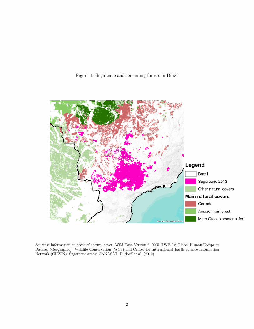
Figure 1: Sugarcane and remaining forests in Brazil
Sources: Esri, USGS, NOAA
LegendBrazilSugarcane 2013Other natural covers
Main natural coversCerradoAmazon rainforestMato Grosso seasonal for.
Sources: Information on areas of natural cover: Wild Data Version 2, 2005 (LWP-2): Global Human FootprintDataset (Geographic). Wildlife Conservation (WCS) and Center for International Earth Science InformationNetwork (CIESIN). Sugarcane areas: CANASAT, Rudorff et al. (2010).
3

preparation, an increase in price perceived as permanent generates different incentives interms of sugarcane planting and replanting than transitory price shocks. In this industry,such clean permanent price changes are hard to see in the data. My approach is to usevariation in agricultural profitability and replanting patterns to estimate a model that allowsme to disentangle the effects of permanent price changes on the intensive (yield) and extensive(acreage) margins.
I incorporate both adoption of sugarcane and replanting in a single dynamic model. Inthe model, farmers planting sugarcane must decide at every period either to replant theirsugarcane fields or not. If they do not replant, expected yields decline next period. If theychoose to replant, they pay a fixed replanting cost and sugarcane yields are restored. Thisfeature makes this problem similar to optimal machine replacement (Rust, 1987).3 Farmersalways have the option of switching away from sugarcane production to other uses. Meanwhile,farmers not planting sugarcane must decide at every period whether to plant sugarcane ornot. Payoffs from both sugarcane and other uses depend on prices that are allowed to evolvestochastically.
I estimate the model using a unique remote sensing dataset of sugarcane land use in Brazilfrom the CANASAT project (Rudorff et al., 2010). The project processes satellite imagesfrom Landsat to provide detailed maps of sugarcane field activity for the most importantsugarcane producing region of Brazil. I complement this land use data with GAEZ/FAOhigh-resolution potential yield information and other detailed field level land characteristics.Given the sparsity of good transportation network in remote areas of Brazil, transportationcosts are an important source of variation in agricultural profitability. Therefore, I model aquality-adjusted transportation network, which is used to measure the transportation cost todestination markets.
I use the model estimates to decompose the sugarcane supply elasticity into farmlandexpansion (extensive margin) and yield (intensive margin) components. I find a long-runyield elasticity of 0.27, comparable to what is believed an upper bound for most annual cropsin developed countries.4 However, I find a value for the long-run acreage elasticity of 4.38,which is a different order of magnitude compared to the yield elasticity. The combined effectsof acreage and yield translates into a high supply elasticity, which suggests small price effectsfrom demand shifts. The high acreage to yield elasticity ratio I find means that, as we movealong the supply curve, 94% of new ethanol comes from expansion in farmland and only 6%from yield increase that accrues from a faster replanting rate.
The high long-run acreage elasticity found here contrasts with existing measures of acreageprice responses in the literature. Roberts and Schlenker (2013) measure short-run demand
3There is also an interesting parallel with optimal oil drilling (Kellogg (2014), Anderson et al. (2014)), asoil well productivity also decays exponentially as well pressure recedes.
4See Berry (2011), Scott (2013b) and Miao et al. (2015) for discussions on the potential range for annualfood crops yield-price elasticities.
4

and supply elasticities for food crops and find inelastic demand and supply. Scott (2013a)estimates the acreage elasticity using a dynamic model and US land use data. He finds a higherlong-run acreage elasticity once forward-looking behavior is taken into account. However, theacreage elasticity found by Scott (2013a) is still an order of magnitude lower than the acreageelasticity I find for sugarcane in Brazil. This difference can be due in part to the very activeBrazilian agricultural frontier compared to the already consolidated American farmland. Thishighlights the danger of extrapolating measures of acreage elasticity from one country toanother when evaluating land use changes. Using American numbers for long run acreageresponses in Brazil would imply that 45% of new ethanol at the margin would come fromyield increases. This would severely understate the environmental costs of biofuels policies asa smaller fraction of new ethanol would be coming from expansion in farmland.
The high-resolution nature of the data together with the estimated model allows me tomake predictions about which types of land cover are affected by sugarcane expansion. Outof the total farmland expansion, 12% is predicted to be over forests and other types of naturalcover, with the Cerrado ecosystem and the southern fringe of the Amazon rainforest beingthe most affected. Deforestation can be magnified by indirect land substitution as sugarcanetakes over other cropland and pasture. The expansion of sugarcane in areas with previousagricultural use decreases the supply of other agricultural products and is expected to causefurther expansion of farmland as the market re-equilibrates at a higher price level.
I use available empirical evidence to quantify these indirect effects in deforestation. Inorder to put this predicted deforestation in perspective, I balance the carbon released bydirect and indirect deforestation and the carbon saved by replacing fossil fuels. I find that newethanol “pays back” in terms of carbon in about 20 years. In contrast, corn ethanol producedin the US is expected to “pay back” in 167 years (Searchinger et al., 2008). Currently there isno consensus about payback times for sugarcane ethanol. Estimates of the sugarcane ethanolcarbon payback time vary from 4 to more than 100 years in the scientific literature, dependingon the type of land cover affected (Elshout et al. (2015), Gibbs et al. (2008), Fargione et al.(2008)). In this paper, I compute a carbon payback time that brings together the economicsof land use and the current scientific knowledge about emissions from land use change.
As an illustrative policy experiment, I discuss the implications of current U.S. RenewableFuel Standard (RFS) for land use in Brazil. The current standard assigns a total of 5 billiongallons in the Advanced Biofuels (ABF) category that need not be met by cellulosic biofuels.This is equivalent to about only 3% of the U.S. annual gasoline consumption. As of now,Brazilian sugarcane ethanol is the only viable large scale alternative to fill the ABF mandate.I find that a 5 billion gallons shift in the market demand for sugarcane ethanol would implya modest 1% price increase, but about 2,000 sq. km in direct deforestation. This could bemagnified to 9,000 sq. km (~ 3/4 the size of Connecticut) if indirect effects are considered.
This is not the first study to investigate the implications of ethanol policies in the context
5

of Brazilian sugarcane ethanol (e.g., De Gorter et al. (2013), Elobeid and Tokgoz (2008), Lascoand Khanna (2010) and Nagavarapu (2010)). Other studies in the literature use mainly staticgeneral equilibrium to evaluate the effects of policies in the markets for sugar and ethanol usingsupply elasticities derived from short-run responses to prices. An exception is Nagavarapu(2010), which estimates a static general equilibrium model for land use and labor allocation inthe sugarcane industry in Brazil using micro level data on the worker decision, but aggregatedata on land use.
The rest of the paper is organized as follows. Section 2 presents a short background of thesugarcane industry in Brazil. Section 3 describes in more detail the land use model. Section4 presents the data and some descriptive analysis. Section 5 discusses the model estimation.Counterfactuals are discussed in Section 6. Section 7 concludes.
2 Industry background
Sugarcane has long history in Brazil, dating back to colonial times. Once sugar was the mostimportant export commodity in the country, but its importance for the Brazilian economyhas faded away over time. In the aftermath of the seventies oil shocks, a government program(PROALCOOL) was created to foster the use of sugarcane ethanol as a replacement forgasoline. Large scale production of sugarcane ethanol has been in place since then. In thepast decade, the emergence of flex-fuel vehicles has given a new boost to the sugarcane ethanolindustry.
Sugarcane has been historically grown close to the coast in Southeast and NortheastBrazil. Today, more than half of sugarcane in Brazil is produced in the State of São Paulo,where physical conditions are ideal for sugarcane growing. In general, suitable conditions forsugarcane include a warm and rainy growing season and a cooler and drier harvest season.The harvest season in the region studied here goes from April to November, depending onthe location and the varieties used. Sugarcane is a semi-perennial crop, which means thatafter plants are cut, if the roots are untouched, a ratoon or stubble crop will follow. However,yields for the ratoon crop are expected to be lower every time this process is repeated (Cragoet al. (2010), Macedo et al. (2008)). For this reason, periodically the field must be replantedso that yields can be restored. Agriculture manuals recommend replanting roughly every 5years.
After harvest, sugarcane is transported to a nearby mill, which is usually located atclose proximity to sugarcane fields. Sugarcane is bulky, so it would be uneconomical to shipcane long distances for milling. Moreover the sugars in the cane deteriorate quickly afterit has been cut, so generally mills are not more than 40 km away from source fields. Atthe mill the sugarcane is crushed and the resulting liquid is either fermented to produceethanol or processed to produce sugar. Modern mills are also thermal electricity generators.
6

They produce electricity by burning leftovers from the crushing process. This innovationsignificantly helped the sugarcane ethanol energy balance (Macedo et al., 2008). Although,there are constant improvements in the milling process, like electricity generation from fibrousmaterials, the milling technology is well known. There is an active market of equipment andmachinery for mills and I know of no technological barriers to entry.
Most modern mills can produce both sugar or ethanol and switch production accordingto market conditions. This technological feature implies that under perfect competition theprice for sugar and ethanol should follow closely together in the medium-run (De Gorter et al.,2013). I consider therefore an unified sugarcane final products market in my analysis, thatincludes both sugar and ethanol as final outputs. As discussed above, most of the controversyregarding sugarcane ethanol is on aspects related to land use and yields and not on emissionsaccruing from the industrial processes, as those are well understood.
3 Model
The unit of analysis is a field indexed by i, which is managed by a profit maximizing farmer.In each year, t, farmers must make a decision regarding land use for the next season. Thisdecision is denoted by qit. If farmers are not planting sugarcane, qit ∈ {plant, stay}, i.e., theycan either plant sugarcane or keep their fields in another economic use. For farmers alreadyplanting sugarcane, qit ∈ {replant, keep, out}, i.e., they can (i) replant the sugarcane fields,(ii) keep the same plants for next season or (iii) switch land use to another activity.
I denote by ait ∈ {0, 1, . . . , a} the state of fields regarding its sugarcane use. If ait = 0,the field is not in sugarcane use, while if ait ≥ 1, the field is in sugarcane use and ait denotesthe sugarcane field age. I denote by wit ∈ W the exogenous state vector, with informationon prices of sugarcane products and alternative crops, land characteristics, transportationcosts and distance to existing sugarcane fields. Finally, there is a state vector εit ∈ R5 whichfarmers observe but not the econometrician.
The flow payoff is given by:
Π(ait, wit, qit, εit; θ) = π(ait, wit, qit; θ) + εit(qit), (1)
where π(ait, wit, qit; θ) is a function that depends only on observed state variables and on avector of parameters to be estimated, θ. Equation 1 makes it clear that for each choice qit,there is a different associated unobserved state εit(qit).
I now describe in more detail π(·; θ). For fields not in a sugarcane use, ait = 0, the flow
7
payoff is given by:
π(0, wit, qit; θ) =
δrit, if qit = stay,
−ΨE(hi, dit; θ), if qit = plant.(2)
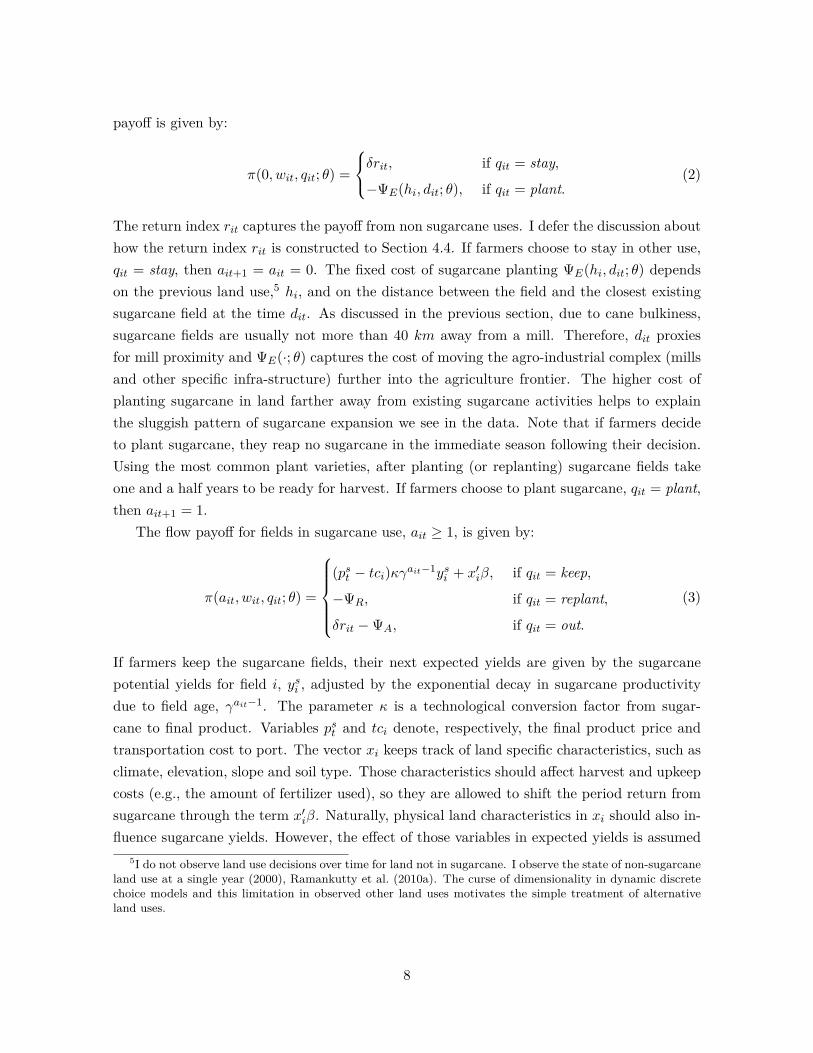
The return index rit captures the payoff from non sugarcane uses. I defer the discussion abouthow the return index rit is constructed to Section 4.4. If farmers choose to stay in other use,qit = stay, then ait+1 = ait = 0. The fixed cost of sugarcane planting ΨE(hi, dit; θ) dependson the previous land use,5 hi, and on the distance between the field and the closest existingsugarcane field at the time dit. As discussed in the previous section, due to cane bulkiness,sugarcane fields are usually not more than 40 km away from a mill. Therefore, dit proxiesfor mill proximity and ΨE(·; θ) captures the cost of moving the agro-industrial complex (millsand other specific infra-structure) further into the agriculture frontier. The higher cost ofplanting sugarcane in land farther away from existing sugarcane activities helps to explainthe sluggish pattern of sugarcane expansion we see in the data. Note that if farmers decideto plant sugarcane, they reap no sugarcane in the immediate season following their decision.Using the most common plant varieties, after planting (or replanting) sugarcane fields takeone and a half years to be ready for harvest. If farmers choose to plant sugarcane, qit = plant,then ait+1 = 1.
The flow payoff for fields in sugarcane use, ait ≥ 1, is given by:
π(ait, wit, qit; θ) =
(pst − tci)κγait−1ysi + x′iβ, if qit = keep,
−ΨR, if qit = replant,
δrit −ΨA, if qit = out.
(3)
If farmers keep the sugarcane fields, their next expected yields are given by the sugarcanepotential yields for field i, ysi , adjusted by the exponential decay in sugarcane productivitydue to field age, γait−1. The parameter κ is a technological conversion factor from sugar-cane to final product. Variables pst and tci denote, respectively, the final product price andtransportation cost to port. The vector xi keeps track of land specific characteristics, such asclimate, elevation, slope and soil type. Those characteristics should affect harvest and upkeepcosts (e.g., the amount of fertilizer used), so they are allowed to shift the period return fromsugarcane through the term x′iβ. Naturally, physical land characteristics in xi should also in-fluence sugarcane yields. However, the effect of those variables in expected yields is assumed
5I do not observe land use decisions over time for land not in sugarcane. I observe the state of non-sugarcaneland use at a single year (2000), Ramankutty et al. (2010a). The curse of dimensionality in dynamic discretechoice models and this limitation in observed other land uses motivates the simple treatment of alternativeland uses.
8

to be fully captured by the potential yield measure ysi .6 Finally, if qit = keep, the sugarcanefield ages in the next season, i.e., ait+1 = min{ait+1, a}. If farmers decide to replant, they paya fixed cost ΨR. Analogously to sugarcane planting, there are no sugarcane related payoffs inthe next season. The replanting decision resets field age: ait+1 = 1. Switching to other usesgives the farmer the return from those other uses, at a fixed land conversion cost ΨA, andsets ait+1 = 0.
In industry discussions, local weather shocks were usually listed as the most importantfactor affecting replanting decisions after sugarcane field age. Particularly bad weather mayincrease the costs of the agricultural operation necessary for field replanting as well as perperiod field upkeep costs. The effects of these weather shocks are captured by the statevariable εit(qit). Moreover, replanting decisions may not always coincide with the optimaldecision from the agronomic point of view. For instance, mills must make sure they have asteady supply of sugarcane, therefore all source fields cannot replant at the same time. Inthis sense, εit(qit) captures the additional noise introduced by other operational concerns.
Assumption 1. The unobserved state variables, εit(q), are independently and identicallydistributed over fields and time.
Assumption 2. The evolution of the exogenous state variables w is not affected by farmersdecisions and ε, i.e., Fwit+1|qit,εit,wit
= Fwit+1|wit.
Assumption 1 is standard in the dynamic discrete choice literature. Assumption 2 embedstwo important underlying features. First, it implies that farmers are price takers, a reason-able assumption for agricultural products markets. Second, it implies that choice specificunobservables ε do not change expectations about the evolution of w.
I assume farmers discount future cash flows using a fixed discount rate ρ < 1. Farmerschoose qit every period conditional on (ait, wit, εit) in order to maximize the sum of futurediscounted flow payoffs:
maxqit
E
∞∑j=0
ρjΠ(ai,t+j , wi,t+j , qi,t+j , εi,t+j ; θ)|ait, wit, εit
.I rewrite below the dynamic optimization problem faced by farmers in the recursive Bell-
man formulation. In a non sugarcane state, a farmer has two options: leave the land in otheruse or convert the land to sugarcane. Therefore, the value function at ait = 0 is
6In the model, I assume farmers use a fixed amount of inputs that gives the maximum attainable yield ysi .
Input choice is an additional margin farmers could use to increase yields. Empirical evidence for high intensityagriculture suggests this margin should be small. For instance, Scott (2013b) finds an upper bound for theyield elasticity of 0.05 from changes in fertilizer use.
9

Vθ(0, wit, εit) = max {π(0, wit, stay; θ) + εit(stay) + ρE [Vθ(0, wit+1, εit+1)|wit] ,
π(0, wit, plant; θ) + εit(plant) + ρE [Vθ(1, wit+1, εit+1)|wit]} . (4)
At 1 ≤ ait ≤ a , which are the productive sugarcane field states, the farmer can either keepthe current field, replant or switch to other use. In this case, the value function is
Vθ(ait, wit, εit) = max {π(ait, wit, keep; θ) + εit(keep) + ρE [Vθ(min{ait + 1, a}, wit+1, εit+1)|wit] ,
π(ait, wit, replant; θ) + εit(replant) + ρE [Vθ(1, wit+1, εit+1)|wit] ,
π(ait, wit, out; θ) + εit(out) + ρE [Vθ(0, wit+1, εit+1)|wit]} . (5)
Assumptions 1 and 2 imply the expected continuation value does not depend on the presentunobserved state εit. Moreover, by Assumption 2, current choices do not alter the distributionof wit+1 conditional on wit. Let vθ(ait, wit, qit) be the deterministic component of each choice’svalue, that is,
vθ(ait, wit, qit) = π(ait, wit, qit; θ) + ρE [Vθ(ait+1(ait, qit), wit+1, εit+1)|wit] ,
where ait+1(ait, qit) denotes the deterministic age transition given current age and choice. Theoptimal choice, or policy function, is given by:
q?θ(ait, wit, εit) = arg maxqvθ(ait, wit, q) + εit(q).
Since εit is unobserved to the econometrician, given observed state variables and param-eters θ, we are not able to precisely determine the optimal choice. We can only recover aconditional choice probability (CCP) given the unobserved state distribution:
Pr(q|ait, wit; θ) =ˆ
1{vθ(ait, wit, q) + εit(q) ≥ vθ(ait, wit, q′) + εit(q′) for all q′}dG(εit).
Assumption 3. εit(q) is independently and identically distributed across alternatives withtype 1 extreme value distribution.
Assumption 3 implies the CCP has the usual logit form:
Pr(q|ait, wit; θ) = vθ(ait, wit, q)∑q′ vθ(ait, wit, q′)
. (6)
The CCP is the basic building block of the likelihood approach I use to estimate themodel’s vector of parameters θ. Aguirregabiria and Mira (2010) provide a great review of
10

dynamic discrete choice models and estimation methods available.
4 Data and descriptive analysis
I combine data from several sources to estimate the model. Here I present these data andprovide a brief discussion of key stylized facts. I begin by describing the construction of thepanel dataset of sugarcane land use. Next, I describe the construction of the distance measureand transportation costs, followed by a brief description of other covariates and its sources.Details are left to Appendix A.
4.1 Tracking sugarcane fields
I use a remote sensing dataset of sugarcane field activity to build the panel of field age {ait}i,t.The CANASAT project mapped sugarcane fields and replanting decisions in the Center Southregion of Brazil for all years between 2004 and 2012 (Rudorff et al., 2010). The maps createdby the CANASAT project are very detailed and sugarcane fields vary in shape and size.
I built the panel dataset of sugarcane activities by creating a 1 km grid of points coveringall the region of interest and tracking land use decisions for each point of the grid over time.7
The grid extends all geographical micro regions8 with sugarcane fields in any sample periodyear. This procedure creates 1,855,224 grid points.
There was a substantial expansion in sugarcane acreage over this sample period. In 2004,less than 1% of the grid points were sugarcane fields. In 2012, this share increased to morethan 4%. Almost half of the sugarcane fields in the region are in the State of São Paulo,which has 25% of its territory covered by sugarcane.
Figure 2 shows one specific producing area in detail. The shapes in the figures are sugar-cane producing fields. They are colored according to the classification given by the CANASATproject. “Ratoon” refers to sugarcane that has not been replanted in the previous cycle; “re-planted” refers to fields that were replanting in the previous cycle; while “replanting” refersto fields being replanted in the current cycle; finally, “expansion” refers to new fields that arefor the first time available for harvest.
Land use decisions are tracked for each grid point over time, creating a panel data ofsugarcane land use. Figure 3 shows the fraction of fields replanted by field age for variouscohorts. The observed mode of replanting is 6 years, which is consistent with industry descrip-tion of replanting decisions. Replanting at higher ages is also frequent, even though not the
7There is no standard way in which this grid should be constructed. As discussed in Scott (2013a), there isa trade-off between oversampling and the amount of extra information a thinner grid would provide. I knowof no existing result on the optimal way of sampling grid points for this type of problem. I believe that the1km choice of grid sparsity is a reasonable compromise between these two forces.
8Micro regions, defined by the Brazilian Institute of Geography and Statistics, are a disjoint set of munici-palities with common social and geographical characteristics.
11

Figure 2: Sugarcane fields in detail
(a) 2011
LegendSugarcane State 2011StateCode
ExpansionReplantingRatoonReplantedGrid points
(b) 2012
LegendSugarcane State 2012StateCode
ExpansionReplantingRatoonReplantedGrid points
Notes: Maps showing a small fraction of the sample region for two different years (2011 and 2012) for illustrativepurposes. The dots in both maps represent the grid points for which sugarcane activities are tracked over time.Colored shapes represent the different classifications given by the CANASAT project.
12

Figure 3: Replanting age by cohort
1 2 3 4 5 6 7 8 9 10 110
0.02
0.04
0.06
0.08
0.1
0.12
0.14
Age
Frac
tion
repl
antin
g
2003
2004
2005
2006
2007
Note: Fraction of existing sugarcane fields that are reported as replanting in each age for different cohorts bythe CANASAT project. The year assigned for each cohort represents the first year the field was available forharvest.
recommended practice by agronomists, who recommend replanting be done not after 5 years.This suggests that achieving higher yields would be possible by increasing the replanting rate.
There is an important caveat about the remote sensing information. Keeping track of thereplanting decision requires the observation of more subtle variation in the satellite imageryat specific moments in the year than what is required to simply identify a sugarcane field.Depending on the variety used or on the time of the year replanting is done,9 the imagingprocess may fail to identify the replanting activity. So it is expected that some fields areerroneously coded as not replanting in a given year, when in fact they were replanted. I dealwith this issue explicitly when estimating the model.
4.2 Distances and transportation cost
I use data on the Brazilian road network from the Ministry of Transportation and the averagespeed on each road type to adjust for road quality. This allows me to measure road distancebetween two points taking into account the quality of the road network on the optimal path.More details about the construction of this transportation network are provided in AppendixA.2. Figure 4 shows the map of the available road network in the Center South Region. Thenetwork is more dense close to the shore and becomes more sparse as we move further into
9In general mills have excess capacity in non-harvest months, so it is not uncommon for some fields to beharvested slightly off season.
13

Figure 4: Road Network
LegendRoad type
HighwayMajor roadUnpaved road
Notes: Map of the road network for South Central Brazil. Own elaboration with road data from the Ministryof Transportation.
the hinterland.The first use of this distance measure is to compute, for each year, the distance of every
grid point to the current closest sugarcane field (variable dit). Figure 5 shows the relationbetween proximity of existing sugarcane fields and the decision to plant sugarcane for the firsttime. There is a sharp decline in the probability of sugarcane adoption as we move away fromexisting fields. This suggests a sluggish pattern of sugarcane expansion, as new sugarcane isusually planted very close to existing fields.
I further use the transportation network to compute transportation costs from every pointin the grid to the closest maritime port. I complement the transportation network with actualfreight quotes to estimate a simple model of transportation costs. I use freight quotes fromSISFRECA (2008), which surveyed transportation quotes for moving sugar from 177 originsto one of three destination ports (Paranaguá, Guarujá and Santos).
The transportation cost model assumes a linear pricing schedule for freight rates. Thereis a fixed rate FC independent of distance traveled and a per kilometer on highway rate V C.Equation 7 describes the total cost of moving commodities from location i to j.
TCij = FC + V C × EffectiveDistanceij + νij , (7)
where EffectiveDistanceij is on highway equivalent distance between i and j, and νij is anerror term, assumed exogenous. I compute effective distances for each one of the 177 origin-
14

Table 1: Transportation cost (2010 US$)
Estimate Std. Err.FC 18.241 1.472V C 0.039 0.003N 177
Notes: Estimated parameters and standard errors from the transportation cost model - Equation (7). Depen-dent variable is transportation cost between cities from SISFRECA (2008). Regressors are the correspondingeffective distances computed using the road network from the Ministry of Transportation and average travelingspeeds from SISFRECA (2008), details for the computation of effective distances in Appendix A.2.
destination pairs using the constructed transportation network and estimate fixed and variablecosts in equation (7). Results are shown in Table 1. I estimate a US$18.24 fixed cost andUS$0.039 per kilometer on highway variable cost of moving one tonne of sugar.
Finally, I compute the effective distances from every point in our grid to the closestmaritime port. I consider as available ports all ports, that according to the Ministry ofTransportation had reported any trading of sugar or ethanol. I use the estimated modeland these effective distances to calculate transportation costs for all grid points (variabletci). Figure 5 shows that grid points with a lower transportation cost to ports had a higherconditional probability of planting sugarcane.
4.3 Other field characteristics
I use as sugarcane potential yield, ysi , the agro-ecological potential yield from FAO/IIASA(2011). FAO provides high-resolution potential yield for a variety of crops for all regions ofthe globe. Those potential yield measures take into account a wide range of soil and climatecharacteristics relevant for agricultural productivity. Figure 5 shows the relation betweenthe measure I use of sugarcane potential yields and sugarcane planting. The conditionalprobability of sugarcane planting increases sharply for at values of potential yields above7 ton. DW/ha. The variation in potential yields shifts the agricultural profitability in asimilarly to permanent price changes. Therefore, this variation will be valuable to estimatethe effects of counterfactual permanent price increases. The noticeable decline in planting atvery high yields highlights the importance of accounting for alternative land uses, as potentialyields for different crops are correlated.
The dataset used to estimate the model is complemented with extensive information onland characteristics described in Table 2, such as climate variables and elevation. Informa-tion on previous land economic use (variable hi) is from Ramankutty et al. (2010a) andRamankutty et al. (2010b), which classified all land in the globe into cropland and pasture.
15

Figure 5: Conditional probability of sugarcane expansion
0 10 20 30 40 50 60 700
0.005
0.01
0.015
Pro
babi
lity
of s
ugar
cane
pla
ntin
g
Effective road distance to closest sugarcane field (km on highway)
50 100 150 200 2500
0.02
0.04
0.06
0.08
0.1
0.12
0.14
Transportation cost (R$/ton)
Pro
babi
lity
of s
ugar
cane
pla
ntin
g
0 2000 4000 6000 8000 100000
0.02
0.04
0.06
0.08
0.1
0.12
0.14
Pro
babi
lity
of s
ugar
cane
pla
ntin
g
Sugarcane yield (DW kg/ha)
Notes: Probabilities of sugarcane adoption conditional on covariates. Adoption refers to new sugarcane growingareas classified by CANASAT. All conditional probabilities smoothed by kernel regression with bandwidthchosen using the rule of thumb at 1.06 × σx × N−1/5. Dotted lines are pointwise 95% confidence intervalscomputed by bootstrap.
16

Table 2: Field characteristics
Variable Mean Std Min Max p20 p50 p80Sugarcane pot. Yield (kg DW/ha) 5791 2273 0 12305 3823 5933 7641
Corn pot. Yield (kg DW/ha) 4247 1971 127 11560 2658 3807 5994Soy pot. Yield (kg DW/ha) 2546 767 0 4443 1943 2645 3241
Transportation cost (US$/ton) 66 26 21 125 42 62 93Dist. to closest sugar field (km) 217.5 256.9 1.0 1589.2 29.1 133.6 335.9
Share in cropland 0.10 0.16 0.00 1.00 0.00 0.03 0.16Share in pasture 0.43 0.28 0.00 1.00 0.13 0.44 0.70
Elevation (m) 518 245 0 2260 305 492 732Prec. growth season (mm) 195.4 44.7 103.8 310.3 153.0 190.8 235.7
Notes: Descriptive statistics of field characteristics. There are 1,855,224 fields (or grid points) in the sample.The characteristics summarized above are available to all fields. Sugarcane, soy and corn potential yields areagroecological potential yields (high inputs) from FAO/IIASA (2011). Transportation cost and distance toclosest sugarcane fields are own elaboration (discussed in text and Appendix A.2) using Ministry of Trans-portation data on roads and survey information from SISFRECA (2008). Cropland and pasture land coverinformation are respectively from Ramankutty et al. (2010a) and Ramankutty et al. (2010b). Climate andelevation data are from Hijmans et al. (2005).
This is a cross-section data on land use for the year 2000.10 I note the higher average share ofpasture (0.43) in our sample area, which has led many11 to believe that most of new sugarcanefields would replace old pasture.
4.4 Prices
As argued in Section 2, I consider one single market for sugarcane final products, that includesboth sugar and sugarcane ethanol. I use the NYSE price of sugar as the reference final productprice. This was was pointed as the relevant reference price for decision making in industrydiscussions. The converted price series to Brazilian Reais (R$) is shown in Figure 6. Theobserved up and downward swings in prices provide variation in agricultural profitability thatis helpful for the estimation of the model.
Equation 8 defines the return index for land not planting sugarcane. It is a weighted sumof the return of alternative agricultural commodities, with the weights given by the relativeimportance of those other crops in the field region:
rit =∑
c∈{corn,soy}pctα
ciyci , (8)
10Unfortunataly, there is no panel remote sensing information that I know of for other crops or pasture forthis region, except for sugarcane.
11See for example EPA (2010).
17

Figure 6: pst (sugar price) and rit (other uses return) series
1995 2000 2005 2010 20150
0.05
0.1
0.15
0.2
0.25
0.3
0.35
0.4
0.45
0.5Sugar price − Sugar #11
Years
R$/
lb.
1995 2000 2005 2010 20150
1000
2000
3000
4000
5000
6000Other uses return − Different estimation bins
Years
R$/
ha.
Notes: Prices used are NYSE future contracts (SB1 for sugar, C1 for corn and S1 for soy) all measured in 2010Reais (R$/lb), deflated using US and Brazilian CPI. All series from 1995 to 2013.
where pct denotes the price of crop c, αci is a measure of the share12 of crop c in the region offield i and yci is the FAO/IIASA potential yield of crop c in field i. Corn and soy correspondto more than half the cropland not in sugarcane in this region. Note that this is a continuousstate variable since potential yield measures are continuous. For practical estimation purposes,I bin the grid points based on cross section categories for rit based on the expected returnsfor the alternative crops. Figure 6 plots the index rit over time for the different estimationbins.
5 Estimation
I estimate the parameters in the model by Maximum Likelihood. The goal of the estima-tion is to recover the vector of parameters θ from observed states {wit, ait}it and decisions{qit}it, where I make the distinction between observed decisions qit and actual decisions qit.This distinction will be more clear shortly. Assumption 2 implies that the evolution of theexogenous state does not depend on current endogenous states or field management decisions.
12Shares of land used for corn and soy are obtained from the 2006 Agricultural Census and refer to MesoAdministrative Regions in the Brazilian Institute of Geography and Statistics (IBGE) classification.
18

Therefore, we can write the conditional log-likelihood criterion function as
L(θ; {qit, wit, ait}it) =∑t
∑i
log f(wit|wit−1; θ) +∑i
log (Pr(qi|wi, ai; θ)) , (9)
where I omit the subscript t to denote the whole vector of decisions and states.Note that the only exogenous state variables in wit that change over time are (pst , rit). For
estimation purposes, I assume (pst , rit) follow an AR(1) process:
[pst
rit
]=[ks
kri
]+[λs 00 λri
] [pst−1rit−1
]+ ηt, (10)
where
ηt ∼ N(
0,σ2s 0
0 σ2ri
).
The exogeneity of the wit transition implies that we can estimate k, λ and σ in a separatefirst step. I then treat those parameters as known when maximizing the second term in thelikelihood function (equation 9) with respect to the payoff parameters. This procedure isdiscussed in more detail now.
The remote sensing exercise may fail to capture replanting if it happens in an unusualperiod of the year or depending on the sugarcane varieties used. This creates classificationerror, as some fields will be classified as not replanting, q = keep, when indeed replantinghappened. If a field is not coded as replanting, I cannot be sure this actually reflects classifi-cation error or just a long sugarcane cycle. If left untreated, this issue could bias upwards ourestimated cost of field replanting. I treat classification error as a field specific unobserved stateui ∈ {1, 2}. If ui = 1, there is no classification error on field i remote sensing observations.In this case, qit = qit, i.e., observed and actual decisions are the same. If ui = 2, replantingdecisions on field i are not observed, that is, qit = keep even when qit = replant. Note thereis only classification error for replanting, the decision to plant sugarcane is not subject toobservational problems. I assume Pr(ui = 1) = µ for all i. We can write the conditionalprobability of observed choices as:
Pr (qi|wi, ai; θ) = µ∏t
Pr (qit|wit, ait, ui = 1; θ) + (1− µ)∏t
Pr (qit|wit, ait, ui = 2; θ) . (11)
The choice probability Pr (·|wit, ait, ui = 1; θ) is exactly the model’s CCP (equation 6) forall ait ∈ {0, 1, . . . , a}, since in this case there is no classification error. However, Pr (·|wit, ait, ui = 2; θ)is only equal to the model CCP when ait = 0, that is, for fields not planting sugarcane. Forait > 0 and ui = 2, only qit = keep is coded, so Pr (keep|wit, ait, ui = 2; θ) = 1.
The model’s CCP depends in principal on the full solution of the dynamic discrete choice
19

problem since vθ(ait, wit, q) depends on the continuation valueE [Vθ(ait+1(ait, qit), wit+1, εit+1)|wit].Solving the dynamic discrete choice problem by value function contraction at every differentlikelihood evaluation is computationally demanding. I use the Nested Pseudo Likelihood(NPL) method proposed by Aguirregabiria and Mira (2002) to circumvent this problem. In-stead of solving the dynamic problem at every different likelihood evaluation, this method usesa single contraction in the space of CCPs. I embed the NPL algorithm with an ExpectationMaximization (EM) step to account for classification error following Arcidiacono and Miller(2011).
Standard errors for payoff parameters are computed by bootstrap. The bootstrap proce-dure follows the estimation steps. For each bootstrap repetition, I re-estimate transportationcosts to ports using a bootstrap sample of freight quotes. Additionally, I re-estimate the tran-sition process (equation 10) using a parametric bootstrap sample of prices. I then re-estimatethe full model with a block bootstrap sample of observations. I discuss estimation details inAppendix B.
5.1 Estimation results
Table 3 shows the estimates for the processes in equation (10). In the first column we presentthe bin number for each category of rit. The second and third column show the values of theweighted yields for corn and soy that define each bin. The other columns show estimates andstandard errors for the auto-regressive processes. The estimated transition for pts is shown atthe bottom of the table.
There is no sign of violation in the stationarity assumption in any of the processes, eventhough standard errors are relatively high. There is a trade-off here between using a longerprice series in dollars and a shorter series measured in the Brazilian currency, Real (R$), whichwas only adopted in 1994. I opt for the second, since this seems to be the appropriate referenceprice, especially in terms of volatility, for decision makers in this market. Moreover, it is notclear that using very old price information adds much to the analysis given changes in marketdynamics in recent decades.13 The cost of relying on relatively recent price information is ashort time series. Imprecision in the estimation of those processes will be taken into accountwhen we compute standard errors for the dynamic model estimates.
In the model section, the functional form for the cost of sugarcane planting, ΨE(hi, dit; θ),was left unspecified. In estimation, I use the following empirical specification for this cost:
ΨE(hi, dit; θ) =∑
l={crop,pasture,other}ψlh1{hi = l}+ ψ1
ddit1{dit ≤ 40}+ ψ2d1{dit > 40}. (12)
13For instance, it was common in the past to observe price spikes whenever there were stock-outs (Deatonand Laroque, 1992). Those type of stock-outs were not seen in recent decades.
20

Table 3: Exogenous state variables transition (std. err.)
(a) rit transition
Est. Bin kri λri σ2ri
1 0.241 (0.144) 0.604 (0.228) 0.010 (0.004)2 0.396 (0.233) 0.561 (0.251) 0.022 (0.009)3 1.208 (0.686) 0.486 (0.285) 0.160 (0.065)4 0.524 (0.307) 0.621 (0.213) 0.051 (0.024)5 0.665 (0.396) 0.603 (0.228) 0.073 (0.034)6 1.444 (0.841) 0.537 (0.262) 0.264 (0.111)7 0.793 (0.462) 0.624 (0.209) 0.122 (0.057)8 0.929 (0.550) 0.614 (0.220) 0.153 (0.071)9 1.681 (0.990) 0.564 (0.250) 0.392 (0.170)
(b) pst transition
ks λs σ2s
0.161 (0.087) 0.482 (0.278) 0.003 (0.001)
Notes: Estimation of the transition process in equation (10). Standard errors (asymptotic) in parenthesis.Prices used are NYSE future contracts (SB1 for sugar, C1 for corn and S1 for soy) all measured in 2010 Reais(R$/lb), deflated using US and Brazilian CPI. All series from 1995 to 2013.
Table 4 shows the results from the NPL estimation of the payoff functions (equations 2and 3) and fixed cost parameters. I find a steep rate of yield decay from sugarcane field age of0.79, which represents an expected yield half life of approximately 3 seasons. Current availableinformation about yield decay for sugarcane is restricted to surveys for specific regions andyears. For instance, Crago et al. (2010) finds a less steep yearly decay rate of 0.86 usingsurvey information restricted to the state of São Paulo in 2007. Their assessment, however,only considers the first 5 harvests. Taking into account that replanting takes one season, adecay rate of 0.79 implies that the replanting age that maximizes average expected yields is3 years. This is in line with recommended agronomic practices, that suggest 3 years as aminimum age for field replanting. However, given the positive fixed cost of replanting, werarely see such short sugarcane cycles, as observed in Figure 3.
I estimate a lower conversion cost for land previously being used for crops in comparisonto land used for pasture or in other use. Consistent with descriptive evidence discussed before,I find a high penalty in the cost of planting sugarcane from the distance to existing sugarcanefields. This penalty implies that the increase in fixed cost associated with moving away fromexisting sugarcane fields by only 10 km is approximately 40% of the revenue associated withthe first sugarcane cut of an average sugarcane field.
21
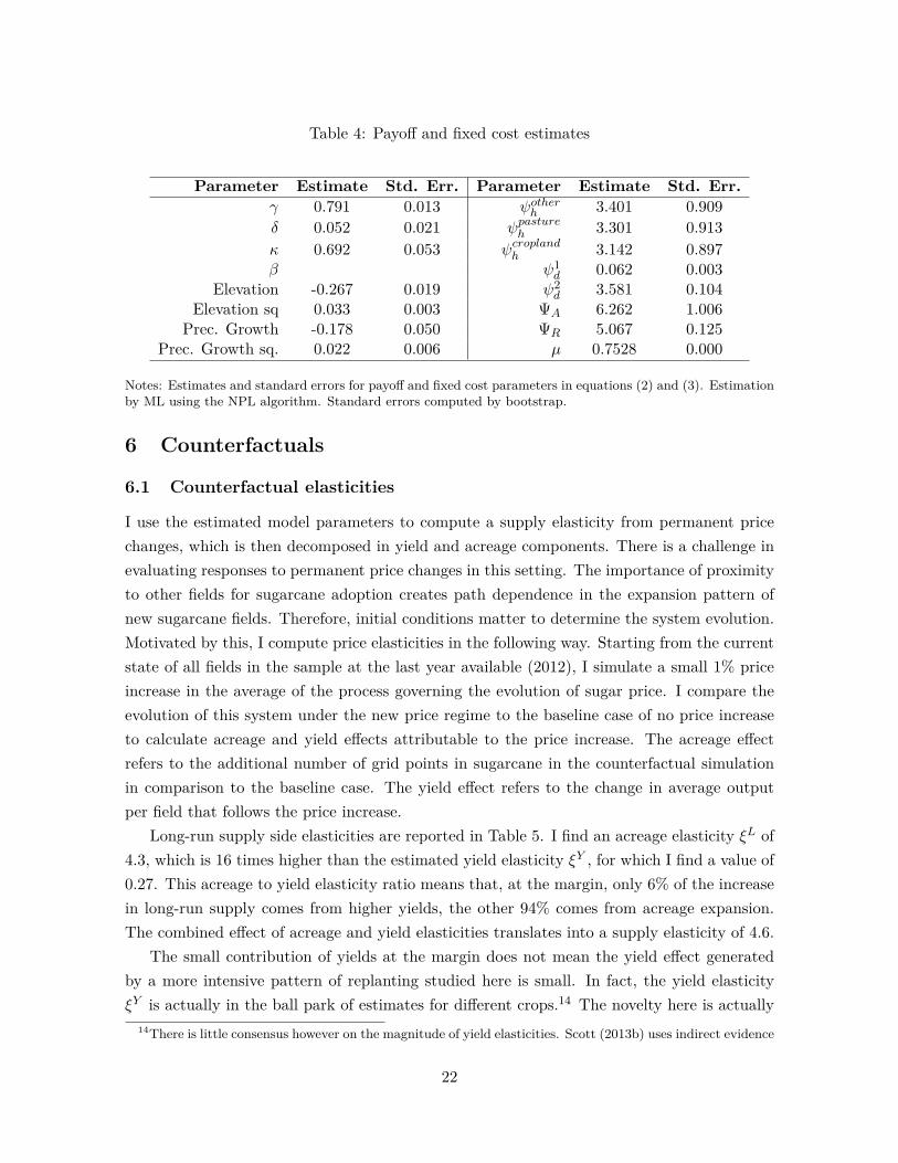
Table 4: Payoff and fixed cost estimates
Parameter Estimate Std. Err. Parameter Estimate Std. Err.γ 0.791 0.013 ψotherh 3.401 0.909δ 0.052 0.021 ψpastureh 3.301 0.913κ 0.692 0.053 ψcroplandh 3.142 0.897β ψ1
d 0.062 0.003Elevation -0.267 0.019 ψ2
d 3.581 0.104Elevation sq 0.033 0.003 ΨA 6.262 1.006
Prec. Growth -0.178 0.050 ΨR 5.067 0.125Prec. Growth sq. 0.022 0.006 µ 0.7528 0.000
Notes: Estimates and standard errors for payoff and fixed cost parameters in equations (2) and (3). Estimationby ML using the NPL algorithm. Standard errors computed by bootstrap.
6 Counterfactuals
6.1 Counterfactual elasticities
I use the estimated model parameters to compute a supply elasticity from permanent pricechanges, which is then decomposed in yield and acreage components. There is a challenge inevaluating responses to permanent price changes in this setting. The importance of proximityto other fields for sugarcane adoption creates path dependence in the expansion pattern ofnew sugarcane fields. Therefore, initial conditions matter to determine the system evolution.Motivated by this, I compute price elasticities in the following way. Starting from the currentstate of all fields in the sample at the last year available (2012), I simulate a small 1% priceincrease in the average of the process governing the evolution of sugar price. I compare theevolution of this system under the new price regime to the baseline case of no price increaseto calculate acreage and yield effects attributable to the price increase. The acreage effectrefers to the additional number of grid points in sugarcane in the counterfactual simulationin comparison to the baseline case. The yield effect refers to the change in average outputper field that follows the price increase.
Long-run supply side elasticities are reported in Table 5. I find an acreage elasticity ξL of4.3, which is 16 times higher than the estimated yield elasticity ξY , for which I find a value of0.27. This acreage to yield elasticity ratio means that, at the margin, only 6% of the increasein long-run supply comes from higher yields, the other 94% comes from acreage expansion.The combined effect of acreage and yield elasticities translates into a supply elasticity of 4.6.
The small contribution of yields at the margin does not mean the yield effect generatedby a more intensive pattern of replanting studied here is small. In fact, the yield elasticityξY is actually in the ball park of estimates for different crops.14 The novelty here is actually
14There is little consensus however on the magnitude of yield elasticities. Scott (2013b) uses indirect evidence
22

Table 5: Long-run elasticities
Supply ξS 4.6158Acreage ξL 4.3372
Yield ξY 0.2721
Notes: Long-run supply elasticities computed by simulating (2000 simulations) the evolution of the fields inour dataset after a 1% price increase.
the very high acreage elasticity. In comparison, Miao et al. (2015) find a corn yield elasticityof 0.23 and an acreage elasticity of 0.45 using US data. In the context of global agriculturesupply, Roberts and Schlenker (2013) find a much lower acreage elasticity of 0.1. Using aforward looking model of land use in the US, Scott (2013a) finds a higher acreage elasticityof 0.3, still much lower than the value found here.
Three effects combine to determine the high acreage elasticity for sugarcane in Brazil Idocument here in comparison to other studies of land use. First, I use a dynamic model toderive the long-run elasticity, while some of the previous studies have only focused on short runacreage responses (Roberts and Schlenker (2013), Miao et al. (2015)). In this sense my resultsgo in the same direction as Scott (2013a), who finds higher acreage price elasticity once forwardlooking behavior is taken into account. Second, as in Miao et al. (2015), this paper focuses on asingle crop, so there is the possibility of cross crop substitution. This is in contrast to Robertsand Schlenker (2013) and Scott (2013a), which aggregate agricultural markets and considerresponses to an aggregate price index. Third, Brazil has a very active agricultural frontier,with large extents of undeveloped land, still shy from realizing its agricultural potential.
In this sense, my results highlight the pitfalls of extrapolating cross-country measures ofacreage elasticity to study land use. Using the acreage elasticity estimated by Scott (2013a)for the US in our analysis would imply that 45% new ethanol at the margin would come fromthe intensive margin. This would imply less expansion in farmland as we move along thesupply curve and thus a downward bias in expected deforestation.
Figure 7 shows the evolution of output, acreage and yield elasticities in the first years afterthe permanent price shock. The permanent price change encourages expansion of sugarcane tonew areas. The expansion of sugarcane in comparison to the baseline translates into acreageelasticities reported in Figure 7. Those new sugarcane fields have higher expected yieldsthan the average pool of sugarcane fields, so yield elasticity jumps in the first periods. Asthose new areas age, the yield elasticity converges to its long-run value, which reflects the moreintensive pattern of replanting that follows the permanent price increase. The output elasticity
from fertilizer use and finds that yield elasticities for corn are unlikely to be larger than 0.04. Miao et al. (2015)presents a good summary of other results in the literature, which range from not statistically significant to0.61, depending on the crop studied and methodological approach.
23

Figure 7: Elasticities on the path to the long-run
1 3 5 7 9 11 13 15 17−1
0
1
2
3
4
5
6
years
elas
ticity
Output
Yield
Acreage
Notes: Output, yield and acreage elasticities path to long-run. Elasticities computed by simulating (2000simulations) the evolution of the fields in our dataset after a 1% price increase.
combines the effects of yield and acreage elasticities. This explains why the output elasticityis steeper than acreage elasticity in the first periods and the faster speed of convergence tothe long-run, in comparison to acreage. Although, the focus of this paper is not the short-run dynamics of this market, it is still interesting to note how the yield and acreage effectsstudied here combine in the short-run to generate a faster response of output in comparisonto acreage.
6.2 Deforestation and carbon “payback” times
The acreage and yield elasticities reported in Table 5 suggest that almost all new sugarcaneproduced following demand shifts in ethanol would come from new growing areas (extensivemargin) and not from more intensive replanting cycles (intensive margin). This is a reasonfor environmental concern, since land use change accounts for a significant part of worldgreenhouse gas emissions.15
In fact, most of the controversy regarding the use of ethanol biofuels comes from the trade-off between the one-shot emission from land conversion and the carbon emissions avoided over
15According to IPCC (2014), deforestation accounted for 12% of global anthropogenic CO2 emissions.
24

time by replacing fossil fuels by a renewable source. A standard measure used to describe thistrade-off is the carbon payback time, i.e., the time it takes for the benefits from replacingfossil fuels to compensate the land use change emissions.16 For the case of sugarcane ethanolthere is little consensus for carbon payback times. This could vary from 5 to more than 100years, depending on assumptions regarding the type of land cover substituted by sugarcane(Searchinger et al. (2008), Elshout et al. (2015), Gibbs et al. (2008), Fargione et al. (2008)).If the land converted to sugarcane fields comes from areas of natural cover with high carbonstorage, e.g., tropical forests, the carbon payback time is going to be high. In turn, if landwith a lower carbon retention is converted, e.g., cropland and pasture, the carbon paybacktime will be smaller.
I use the estimated model to predict the direct effect of sugarcane expansion in differentnatural ecosystems from permanent price shifts. Table 6 shows a decomposition of acreagechanges on different areas of natural cover and on existing cropland and pasture. The firstcolumn reports acreage elasticities of sugarcane for the different land covers. The secondcolumn reports the share of sugarcane predicted by the model in the long-run. The secondto last column shows the share of each type of land converted to sugarcane at the margin inthe long-run.
The last column in Table 6 reports expected carbon emissions from each natural coverfor an 1 km2 sugarcane expansion at the margin.17 Even though the Cerrado region is theone with the highest predicted decrease in natural cover, emissions of the same magnitudeare predicted to come from land conversion of the two ecosystems connected to the Amazonrainforest, the Madeira-Tapajós and Mato Grosso seasonal forests. This reflects the highercarbon density in the Madeira-Tapajós and Mato Grosso forests compared to the Cerrado.
A few caveats are in order. First, the model does not distinguish between areas of nat-ural cover and cleared areas not in cropland or pasture. The predicted expansion reportedignores specific fixed costs of land clearing and environmental regulation that could restrictdeforestation. In this sense, my measure of deforestation and carbon emissions are worse casescenarios. However, this is not the case for pasture and cropland conversion to sugarcane, asI allow the fixed cost of sugarcane planting to vary depending on these two types of land use.Moreover, my analysis focuses only on the Center-South region of Brazil, which includes onlythe Southern fringe of the Amazon rainforest, which is likely to be the most affected by theexpansion of farmland. For a specific treatment of the demand for deforestation in the entireBrazilian Amazon rainforest, see Souza-Rodrigues (2015).
The carbon emission reported in Table 6 represents only direct deforestation by sugarcaneexpansion, which could be aggravated by indirect land use substitution. Note that, out of
16It is important to note that the carbon payback time is not a sufficient measure for a normative analysis.However, several studies of biofuels have used this measure, allowing for comparison across studies.
17The assessment of carbon emissions comes from IPPC guidelines for the evaluation of emissions from landuse change (IPCC, 2006); I leave the details of this computation to Appendix C.
25
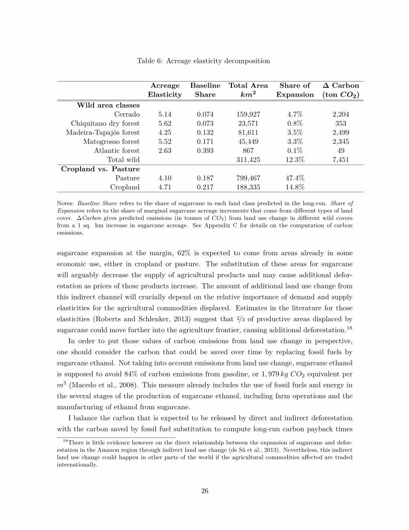
Table 6: Acreage elasticity decomposition
Acreage Baseline Total Area Share of ∆ CarbonElasticity Share km2 Expansion (ton CO2)
Wild area classesCerrado 5.14 0.074 159,927 4.7% 2,204
Chiquitano dry forest 5.62 0.073 23,571 0.8% 353Madeira-Tapajós forest 4.25 0.132 81,611 3.5% 2,499
Matogrosso forest 5.52 0.171 45,449 3.3% 2,345Atlantic forest 2.63 0.393 867 0.1% 49
Total wild 311,425 12.3% 7,451Cropland vs. Pasture
Pasture 4.10 0.187 799,467 47.4%Cropland 4.71 0.217 188,335 14.8%
Notes: Baseline Share refers to the share of sugarcane in each land class predicted in the long-run. Share ofExpansion refers to the share of marginal sugarcane acreage increments that come from different types of landcover. ∆Carbon gives predicted emissions (in tonnes of CO2) from land use change in different wild coversfrom a 1 sq. km increase in sugarcane acreage. See Appendix C for details on the computation of carbonemissions.
sugarcane expansion at the margin, 62% is expected to come from areas already in someeconomic use, either in cropland or pasture. The substitution of these areas for sugarcanewill arguably decrease the supply of agricultural products and may cause additional defor-estation as prices of those products increase. The amount of additional land use change fromthis indirect channel will crucially depend on the relative importance of demand and supplyelasticities for the agricultural commodities displaced. Estimates in the literature for thoseelasticities (Roberts and Schlenker, 2013) suggest that 2/3 of productive areas displaced bysugarcane could move further into the agriculture frontier, causing additional deforestation.18
In order to put those values of carbon emissions from land use change in perspective,one should consider the carbon that could be saved over time by replacing fossil fuels bysugarcane ethanol. Not taking into account emissions from land use change, sugarcane ethanolis supposed to avoid 84% of carbon emissions from gasoline, or 1, 979 kg CO2 equivalent perm3 (Macedo et al., 2008). This measure already includes the use of fossil fuels and energy inthe several stages of the production of sugarcane ethanol, including farm operations and themanufacturing of ethanol from sugarcane.
I balance the carbon that is expected to be released by direct and indirect deforestationwith the carbon saved by fossil fuel substitution to compute long-run carbon payback times
18There is little evidence however on the direct relationship between the expansion of sugarcane and defor-estation in the Amazon region through indirect land use change (de Sá et al., 2013). Nevertheless, this indirectland use change could happen in other parts of the world if the agricultural commodities affected are tradedinternationally.
26

Table 7: Emissions and payback time (1,000L new ethanol)
ILUC scenario 0% 66% 100%CO2 emissions (tonnes) 9.6 41.5 57.9
Payback time (years) 4.8 20.9 29.2
Notes: CO2 equivalent emissions from deforestation and carbon payback times computed under differentassumptions about indirect use substitution. All values computed based on the marginal effects of deforestationreported in Table 6. The x% ILUC scenarios consider the direct emissions plus the emissions corresponding tox% of the displaced area in pasture and cropland on areas of natural cover.
for sugarcane ethanol. Table 7 shows payback times for different assumptions on the magni-tude of the indirect land use change (ILUC). I find 4.8 years payback for sugarcane ethanol,considering only direct deforestation effects. Assuming that 2/3 of the expansion over othercropland and pasture converts into further deforestation, I find a higher payback time of 20.9years. This time could be increased to almost 30 years in the extreme case in which all crop-land and pasture converted to sugarcane ends up expanding into forests. This extreme casewould only be realized if the ratio between supply and demand elasticities for the commoditiesdisplaced by sugarcane is infinite. This extreme case provides a reasonable upper bound forthe sugarcane ethanol carbon payback time.
The sensitivity of the carbon payback times to indirect land use change computed heremerits extra attention and should be a topic of future research. The deforestation fromindirect land use change might be pivotal in a welfare assessment of sugarcane ethanol policies.However, the carbon payback times in any scenario are dwarfed compared to US corn ethanol,which pays back in 167 years (Searchinger et al., 2008). This difference is primarily due to alower carbon efficiency in corn ethanol production in comparision to sugarcane.
6.3 Ethanol mandates
In this section I use the estimated model to discuss the effects of biofuels policies. There is arange of ethanol policies in the world today. Here I focus on the most common ones: thosethat shift the demand for ethanol by establishing ethanol blending standards in transportationfuel. Brazil, like many countries, establishes a fixed proportion of ethanol blend in gasoline.Although some States in the U.S. have similar rules, the Federal policy establishes only anaggregate volume of ethanol to be blended to gasoline every year. For simplicity, I study herethe effects of shifts in the demand curve for ethanol that would be implied by those mandates.
There are some important caveats in the analysis that follows. First, the results so far con-cern only the supply side of sugarcane ethanol. Evaluating the effects of demand shifts in thismarket will require some knowledge of the demand side. I do not estimate a demand elasticityin this paper; instead, I rely on existing results from the literature and assess the robustness
27

Table 8: U.S. 2007 Renewable Fuel Standard (Billions of gallons)
Total Advanced Cellulosicvolume biofuels biofuels
2014 18.15 3.75 1.752018 26 11 72022 36 21 16
of my findings. Second, I estimate the long-run price increase that follows the demand shiftusing a static equilibrium model. This is in contrast to my measure of supply elasticity thatwas derived using a dynamic model. I believe that a static equilibrium framework provides aparsimonious environment to study the long-run effects of ethanol mandates.
As an illustrative policy experiment, I consider the effect of the 2007 EISA,19 whichestablishes increasing mandates for ethanol in a nested system. EISA sets an increasing totalmandate for renewable fuels from 18 billion gallons in 2014 to 36 billion gallons in 2022 butis subject to EPA rulemakings, which can allow for lower standards each year.20 Table 8describes the mandated volumes of biofuels for selected years. The first column shows thetotal volume of biofuels to be blended. The second column defines the amount that mustbe met with advanced biofuels and the third column, the amount of the advanced biofuelsmandate that must be met by cellulosic biofuels.
In order to meet the mandate, biofuels must achieve at least a 20% reduction in life cyclegreenhouse21 emissions in comparison with gasoline and diesel. Under the non-advancedbiofuel category falls almost all corn based ethanol produced in the US. Advanced biofuelsmust achieve at least a 50% reduction in greenhouse gas emissions in comparison with fossilfuels. Finally, cellulosic biofuels refer to biofuels derived from any cellulose that achieve a 60%gain in terms of greenhouse gas emissions. There was not much interest from the private sectorin cellulosic ethanol mainly because the necessary conversion technology is still too costly forlarge scale application (Bracmort, 2012). As consequence, EPA has been continuously usingits statutory authority to the waive cellulosic biofuels mandate on the basis of “insufficientsupply.”
Brazilian sugarcane ethanol is classified by the EPA as an advanced biofuel. In fact, it19Energy Independence and Security Act.20The EPA has the stutory authority to waive the biofuels mandate in the cases of “insufficient supply” or
“economic harm.” For example, in 2014 the EPA set the final volume of ethanol in the standard to 15.9 billiongallons, below the volume predicted in EISA. It is likely that EPA will continue to set lower stadard volumesof ethanol in the following years.
21According to EISA 2007 sec. 201, “‘lifecycle greenhouse gas emissions’ means the aggregate quantityof greenhouse gas emissions (including direct emissions and significant indirect emissions such as significantemissions from land use changes), as determined by the Administrator, related to the full fuel lifecycle, includingall stages of fuel and feedstock production and distribution, from feedstock generation or extraction throughthe distribution and delivery and use of the finished fuel to the ultimate consumer, where the mass values forall greenhouse gases are adjusted to account for their relative global warming potential.”
28

Table 9: Effects of sugarcane ethanol mandates
5 billion gallons mandate
Mandate/World output: 6.45%Mandate/Brazil output: 9.71%
Demand elasticity -0.05 -0.2 -0.9∆ % price 1.38% 1.33% 1.16%∆ % yield 0.37% 0.36% 0.31%
∆ Total Acreage (km2) 17,830 17,277 15,093−∆ Natural (km2) 2,202 2,133 1,864
Notes: Aggregate effects of a 5 billion gallons sugarcane ethanol mandate. Mandate share of world and Braziloutput were calculated using FAOSTAT 2013 information of sugarcane total output and the model baselinepredicted change in Brazilian supply. We use 86.3 L/tonne of cane (Macedo et al., 2008).
is the sole large scale source of Advanced Biofuels in the EPA classification. I consider acounterfactual shift in the world demand of sugarcane ethanol of 5 billion gallons, whichis the volume in the advanced biofuel category that needn’t be met by cellulosic biofuels(21− 16 = 5, in 2022, Table 8).
Table 9 shows aggregate effects on prices, acreage expansion and yields in Brazil of a 5billion gallons mandate of sugarcane ethanol. I use a baseline demand elasticity of −0.2 fromElobeid and Tokgoz (2008).22 Policy effects are not sensitive to demand elasticities in theinelastic range. The low price responses and comparatively high acreage responses are drivenprimarily by the high acreage to yields elasticity ratio I find. This analysis suggests that a 5billion gallon mandate, which is equivalent to about 3% of US gasoline consumption, couldimply about 2,000 sq. kilometers in direct deforestation. Following the previous analysis ofindirect deforestation, this could be magnified to 9,000 sq. kilometers if indirect effects areconsidered.
7 Conclusion
This paper studies the economics of land use for the sugarcane ethanol production to quan-tify the environmental effects of biofuel policies. The expansion in ethanol production mayendanger tropical forests, which could offset the carbon savings accrued over time by thereplacement of fossil fuels. I use a dynamic model of land use that encompasses both adop-tion of sugarcane and replanting decisions, which is crucial to disentangle acreage and yieldresponses to policy changes.
I find a high acreage-price elasticity, which implies much higher acreage to yield elasticityratios than found in previous studies. The results suggest that ad-hoc assumptions on the
22Roberts and Schlenker (2013) find a comparable values of demand elasticities for agricultural products.
29

pattern of land expansion can severely bias the evaluation of the merits of sugarcane ethanolas a greener replacement for fossil fuels. The most detrimental environmental effects frombiofuels demand shifts come from land use change associated with an expansion of biofuelscrops. If the acreage to yield elasticity ratio is low, there is scope for yields to absorb theincrease in demand. However, if the acreage elasticity is higher than the yield elasticity, theincrease in ethanol supply comes primarily from new producing areas.
In the case of Brazilian sugarcane ethanol, I find that the extensive margin (acreage)dominates the intensive margin (yield). This results in large acreage expansion followingan increase in feedstock demand and a comparatively small increase in yields. I use thehigh-resolution nature of the dataset and the estimated model to predict the direct effectson natural land cover and associated carbon emissions. I discuss how indirect deforestationcaused by crop and pasture substitution could aggravate land use change emissions. I findlower carbon payback times for sugarcane ethanol compared to US corn ethanol, but theseare somewhat sensitive to the importance of indirect land use change, which points in thedirection of important future research.
References
Victor Aguirregabiria and Pedro Mira. Swapping the nested fixed point algorithm: A classof estimators for discrete Markov decision models. Econometrica, 70(4):1519–1543, 2002.
Victor Aguirregabiria and Pedro Mira. Dynamic discrete choice structural models: A survey.Journal of Econometrics, 156(1):38–67, 2010.
Treb Allen and Costas Arkolakis. Trade and the topography of the spatial economy. TheQuarterly Journal of Economics, 129(3):1085–1139, 2014.
Soren T Anderson, Ryan Kellogg, and Stephen W Salant. Hotelling under pressure. NBERWorking Paper, (20280), 2014.
Peter Arcidiacono and Robert A Miller. Conditional choice probability estimation of dy-namic discrete choice models with unobserved heterogeneity. Econometrica, 79(6):1823–1867, 2011.
Steven Berry. Biofuels policy and the empirical inputs to GTAP models. Discussion Paper,2011.
Kelsi Bracmort. Meeting the renewable fuel standard (RFS) mandate for cellulosic biofuels:Questions and answers. CRS Report for Congress, (R41106), 2012.
30

Christine L Crago, Madhu Khanna, Jason Barton, Eduardo Giuliani, and Weber Amaral.Competitiveness of Brazilian sugarcane ethanol compared to US corn ethanol. EnergyPolicy, 38(11):7404–7415, 2010.
Harry De Gorter, Dusan Drabik, Erika Kliauga, and Govinda R Timilsina. An economicmodel of Brazil’s ethanol-sugar markets and impacts of fuel policies. World Bank PolicyResearch Working Paper, (6524), 2013.
Saraly Andrade de Sá, Charles Palmer, and Salvatore Di Falco. Dynamics of indirect land-use change: empirical evidence from Brazil. Journal of Environmental Economics andManagement, 65(3):377–393, 2013.
Angus Deaton and Guy Laroque. On the behavior of commodity prices. The Review ofEconomic Studies, 59(1):1–23, 1992.
Amani Elobeid and Simla Tokgoz. Removing distortions in the US ethanol market: What doesit imply for the United States and Brazil? American Journal of Agricultural Economics,90(4):918–932, 2008.
PMF Elshout, R van Zelm, J Balkovic, M Obersteiner, E Schmid, R Skalsky, M van derVelde, and MAJ Huijbregts. Greenhouse-gas payback times for crop-based biofuels. NatureClimate Change, 2015.
EPA. Renewable Fuel Standard Program (RFS2) Regulatory Impact Analysis. 2010.
FAO/IIASA. Global Agro-ecological Zones (GAEZ v3.0). FAO and IIASA, Rome, Italy andLaxenburg, Austria, 2011.
Joseph Fargione, Jason Hill, David Tilman, Stephen Polasky, and Peter Hawthorne. Landclearing and the biofuel carbon debt. Science, 319(5867):1235–1238, 2008.
Holly K Gibbs, Matt Johnston, Jonathan A Foley, Tracey Holloway, Chad Monfreda, NavinRamankutty, and David Zaks. Carbon payback times for crop-based biofuel expansion inthe tropics: The effects of changing yield and technology. Environmental Research Letters,3(3):034001, 2008.
R.J. Hijmans, S.E. Cameron, J.L. Parra, P.G. Jones, and A. Jarvis. Very high resolutioninterpolated climate surfaces for global land areas. International Journal of Climatology,25:1965–1978, 2005.
V Joseph Hotz and Robert A Miller. Conditional choice probabilities and the estimation ofdynamic models. The Review of Economic Studies, 60(3):497–529, 1993.
31

IPCC. 2006 IPCC Guidelines for National Greenhouse Gas Inventories, volume 4. IPCC,Hayama, Japan, 2006.
IPCC. Climate Change 2014: Mitigation of Climate Change. Contribution of Working GroupIII to the Fifth Assessment Report of the Intergovernmental Panel on Climate Change.Cambridge University Press, Cambridge, UK, 2014.
Ryan Kellogg. The effect of uncertainty on investment: Evidence from Texas oil drilling. TheAmerican Economic Review, 104(6):1698–1734, 2014.
Christine Lasco and Madhu Khanna. US-Brazil trade in biofuels: Determinants, constraints,and implications for trade policy. In Handbook of Bioenergy Economics and Policy, pages251–266. Springer, 2010.
Isaias C Macedo, Joaquim EA Seabra, and João EAR Silva. Green house gases emissions inthe production and use of ethanol from sugarcane in Brazil: The 2005/2006 averages anda prediction for 2020. Biomass and bioenergy, 32(7):582–595, 2008.
Ruiqing Miao, Madhu Khanna, and Haixiao Huang. Responsiveness of crop yield and acreageto prices and climate. American Journal of Agricultural Economics, 2015.
Sriniketh Nagavarapu. Implications of unleashing Brazilian ethanol: trading off renewablefuel for how much forest and savanna land. Working Paper, 2010.
N. Ramankutty, A.T. Evan, C. Monfreda, and J.A. Foley. Global Agricultural Lands:Croplands, 2000. Data distributed by the Socioeconomic Data and Applications Cen-ter (SEDAC): http://sedac.ciesin.columbia.edu/es/aglands.html. (Accessed 09/19/2014).,2010a.
N. Ramankutty, A.T. Evan, C. Monfreda, and J.A. Foley. Global Agricultural Lands: Pasture,2000. Data distributed by the Socioeconomic Data and Applications Center (SEDAC):http://sedac.ciesin.columbia.edu/es/aglands.html. (Accessed 09/19/2014)., 2010b.
Michael J. Roberts and Wolfram Schlenker. Identifying supply and demand elasticities ofagricultural commodities: Implications for the US ethanol mandate. American EconomicReview, 103(6):2265–2295, 2013.
B. F. T. Rudorff, D. A. Aguiar, W. F. Silva, L. M. Sugawara, M. Adami, and M. A. Moreira.Studies on the rapid expansion of sugarcane for ethanol production in São Paulo State(Brazil) using landsat data. Remote sensing, 2(4):1057–1076, 2010.
John Rust. Optimal replacement of GMC bus engines: An empirical model of Harold Zurcher.Econometrica, 55(5):999–1033, 1987.
32
Paul T. Scott. Dynamic discrete choice estimation of agricultural land use. Working Paper,2013a.
Paul T. Scott. Indirect estimation of yield-price elasticities. Working Paper, 2013b.
Timothy Searchinger, Ralph Heimlich, Richard A Houghton, Fengxia Dong, Amani Elobeid,Jacinto Fabiosa, Simla Tokgoz, Dermot Hayes, and Tun-Hsiang Yu. Use of US croplandsfor biofuels increases greenhouse gases through emissions from land-use change. Science,319(5867):1238–1240, 2008.
SISFRECA. SISFRECA 2008 Yearbook. ESALQ-LOG, Piracicaba, Brazil, 2008.
Eduardo A. Souza-Rodrigues. Deforestation in the Amazon: A unified framework for estima-tion and policy analysis. Working Paper, 2015.
A. Valente, V. Tani, A. Coelho, M. Pimenta, P. Tome, R. Reibnitz, and R. Queiroz. Deter-minacao das velocidades médias de operacao para o ano de 2006. Technical report, 2008.
33
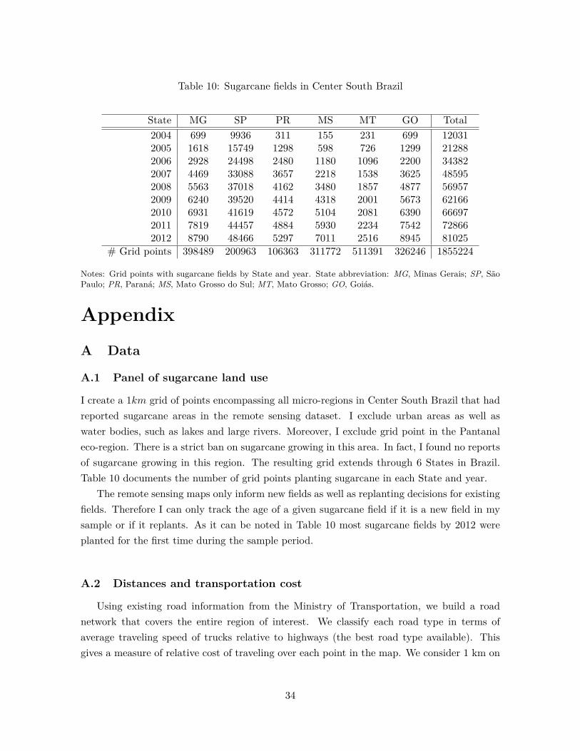
Table 10: Sugarcane fields in Center South Brazil
State MG SP PR MS MT GO Total2004 699 9936 311 155 231 699 120312005 1618 15749 1298 598 726 1299 212882006 2928 24498 2480 1180 1096 2200 343822007 4469 33088 3657 2218 1538 3625 485952008 5563 37018 4162 3480 1857 4877 569572009 6240 39520 4414 4318 2001 5673 621662010 6931 41619 4572 5104 2081 6390 666972011 7819 44457 4884 5930 2234 7542 728662012 8790 48466 5297 7011 2516 8945 81025
# Grid points 398489 200963 106363 311772 511391 326246 1855224
Notes: Grid points with sugarcane fields by State and year. State abbreviation: MG, Minas Gerais; SP, SãoPaulo; PR, Paraná; MS, Mato Grosso do Sul; MT, Mato Grosso; GO, Goiás.
Appendix
A Data
A.1 Panel of sugarcane land use
I create a 1km grid of points encompassing all micro-regions in Center South Brazil that hadreported sugarcane areas in the remote sensing dataset. I exclude urban areas as well aswater bodies, such as lakes and large rivers. Moreover, I exclude grid point in the Pantanaleco-region. There is a strict ban on sugarcane growing in this area. In fact, I found no reportsof sugarcane growing in this region. The resulting grid extends through 6 States in Brazil.Table 10 documents the number of grid points planting sugarcane in each State and year.
The remote sensing maps only inform new fields as well as replanting decisions for existingfields. Therefore I can only track the age of a given sugarcane field if it is a new field in mysample or if it replants. As it can be noted in Table 10 most sugarcane fields by 2012 wereplanted for the first time during the sample period.
A.2 Distances and transportation cost
Using existing road information from the Ministry of Transportation, we build a roadnetwork that covers the entire region of interest. We classify each road type in terms ofaverage traveling speed of trucks relative to highways (the best road type available). Thisgives a measure of relative cost of traveling over each point in the map. We consider 1 km on
34

Figure 8: Predicted transportation cost and effective distance
0 500 1000 1500 2000 25000.04
0.06
0.08
0.1
0.12
0.14
0.16
Effective distance (km in highway)
Ave
rage
cos
t (U
S$/
ton
× km
)
Notes: Predicted average (per km) transportation cost from the estimated transportation cost equation (7).Actual average freight rates from SISFRECA (2008) and effective distance measure used in estimation areshown scattered.
highway to be equivalent to 1.25 km on a major road, 1.66 km on unpaved road and 2.5 kmeverywhere else. Those values are informed by Valente et al. (2008), which surveys travelingspeed of different types of vehicles. As an example, suppose the best route between i and j is1 km on a dirt road, then we consider that effective distance between i and j to be 1.66 km.
From this measure of relative traveling cost, we search for the cheapest path given thedifferent costs of traversing each parcel. This is implemented using ArcGIS cost distancetools. For an excellent description of this type of least cost path algorithm, see Allen andArkolakis (2014).
Since we use the estimated transportation cost model (equation 7) to extrapolate freightrates for all points in the grid, it is important that the transportation cost model fits the datawell. In fact, the transportation model fit is reasonably good. Figure 8 examines the fit ofthe transportation cost model, where I plot predicted transportation cost by the model in thesolid line and actual quotes.
The calculated map of transportation costs is shown in Figure 9. We can see a big variationin projected transportation costs to the closest port ranging from US$18 per tonne close todestination ports to more than US$100 per tonne on the agriculture frontier. I extract the
35

Figure 9: Sugar transportation cost to nearest port (tci)
"
#
!
Legend Mains Ports SE
! Paranaguá" Rio de Janeiro# Santos
Sugar transportation costUS$/ton
High : 161.006
Low : 18.241
Notes: Sugar transportation cost (US$/ton) and main destination ports in South Central Brazil. Variable tci
in equation 3. Transportation cost is calculated for each grid point using the estimated transportation costmodel; equation (7) and Table 1.
value of transportation cost from this map for every point in the grid.A.3 Other land characteristics
Potential yields (yci ). I use agro-ecological potential yields from FAO/IIASA (2011), v3.0.GAEZ provides potential yield infomation for different levels of input use and irrigation sys-tem. For all crops, c, I use values for rain-fed and high-input use. Figure 10 depicts thesugarcane potential yield information. A high yield region is noticeable where most currentsugarcane fields are located in the center of the map. There is also a high yield area to thenorth of the map that coincides with the Southern fringe of the Amazon rainforest.
Previous economic use (hi). I use information on previous economic land uses from Ra-mankutty et al. (2010a) and Ramankutty et al. (2010b). This dataset informs for every pointin the globe a predicted probability that the land is covered by pasture and the probabilitythe land is covered by cropland. Those probabilities are informed at a 10 km resolution. Inmodel estimation, I draw for every grid point a land cover (cropland, pasture or other) usingthe probabilities informed by the dataset.
Climate and elevation (xi). Climate and elevation are extracted for all grid points fromHijmans et al. (2005). This is a high-resolution climate dataset with information on monthlytemperature and rainfall. This climate information is too rich to be used fully in estimation.
36

Figure 10: Sugarcane potential yield (yis)
LegendBrazil
GAEZ/FAO sugarcane yieldkg DW/ha
High : 13647
Low : 0
Notes: Sugarcane agro-ecological potential yield (high inputs). Source: FAO/IIASA (2011).
I use averages over the growth (Nov-Apr) and harvest seasons (May-Oct) of those climatevariables climate variables in estimation.
B Estimation
Structural parameters in the payoff functions are estimated using the Nested Pseudo Like-lihood (NPL) algorithm proposed by Aguirregabiria and Mira (2002). The algorithm is mod-ified to incorporate misreports in replanting in the spirit of Arcidiacono and Miller (2011).
The processes that govern the evolution of the sugar price and outside options return areestimated offline. The NPL algorithm builds on the method proposed by Hotz and Miller(1993), which suggest a clever use of Conditional Choice Probabilities (CCP) to reduce thecomputational burden imposed by “full solution” alternatives, e.g., the Nested Fixed Pointalgorithm (Rust (1987)).
Aguirregabiria and Mira (2002) show that in many dynamic discrete choice problems thereis a contraction mapping in the space of conditional choice probabilities:23
p = Υθ(p),
where the contraction mapping is naturally dependent on the vector of parameters describing23This is analogous to the contraction mapping in the space of value functions.
37

the optimization problem θ.The algorithm I use is a modification of NPL proposed by Arcidiacono and Miller (2011)
that is used here to control for misreports in replanting. Given technical difficulties in theclassification of replanting, for some fields that replant will not have this activity coded inour panel dataset. We consider two types of regime. A field can either not be subject tomisreport in replanting (ui = 1), in which case whenever replanting happens, this activity willbe observed in the dataset, or it can be subject to misreport in replanting (ui = 2), in whichcase I will not see replanting in case it happens. There is no indication of classification error inthe adoption of sugarcane. Let µ be the probability there is no classification error. Naturally,1− µ denote the probability in the population that a field is subject to classification error. µis treated as unknowns and estimated by Maximum Likelihood with the other parameters.
I now describe the estimation algorithm. Let qi denote the observed decisions for fieldi. Start the algorithm at step K = 0 with an initial try of the CCP estimate p0 and forPr(ui = u) = µu0 , for u ∈ {1, 2}. For every step K ≥ 1,
1. Update each field regime ex-post probability using Bayes rule:
Pr (ui = u|qi, ωi, ai) =µuK−1pK−1(qi|ωi, ai, u)∑
u={1,2} µuK−1pK−1(qi|ωi, ai, u) , for u = 1, 2.
2. Compute estimates of payoff parameters
θK = arg maxθ
n∑i=1
∑u={1,2}
Pr (ui = u|qi, ωi, ai) ln Υθ(pK−1)(qi|ωi, ai, u). (13)
3. Use estimates θK to update the CCPs:
pK = ΥθK(pK−1).
4. Update µ1 and µ2:
µuK = 1N
N∑i=1
Pr (ui = u|qi, ωi, ai) , for u = 1, 2.
5. Iterate until convergence in p, θ and µ is reached.
Note that if replanting was observed for a given field i, then pK(qi|ωi, ai, 2) = 0, and soPr (ui = 1|qi, ωi, ai) = 1. Moreover, fields in the replanting classification error regime have,naturally, zero probability of having replanting coded, hence pK(qi|ωi, ai, 2) = 1. Existingsugarcane fields in the beginning of the sample for which replanting was never observed in the10 years of data available are treated as being in the classification error state, ui = 2. This
38

Table 11: Estimation settings
ρ 0.9a 9
Discrete state space:Transp. cost (R$/lb) 0.027 0.043 0.058 0.084
Dist. to closest sugar field (km) 1.5 9.0 27.5 >40ys (kg DW/ha) 2119 5089 6601.5 9784.5
Altitude (m) 168.5 414 586.5 1484Prec. Growth Season (mm) 131.3 174.8 207.0 266.7
ps (R$/lb) 0.188 0.270 0.353 0.435
Notes: Estimation settings for NPL estimation. ρ is the discount factor and a is the cap in sugarcane fieldage. Discretized values for each continuous state variables are shown. With the exception of the distance tosugarcane fields, all classifications are based in equally sparse quantiles, so bins for each discrete category havethe same number of observations.
avoids an initial condition problem for those fields, as we can only observe a field age ai if iis a new field or if it replants. Although there are reports of sugarcane fields going more than10 years without renovation, this is an abnormal situation in this industry.
Intuitively, the algorithm re-weights observations in the likelihood (13), taking into accountthe presence of classification error. For instance, a field with an observed old age that hasnever replanted will have a lower weight in estimation than a younger field that has neverreplanted, conditional on other observables being the same. This is because the former has ahigher ex-post probability of being type u = 2 (classification error) than the latter.
Continuous state variables are discretized for ML estimation purposes. Table 11 showsthe estimation settings, assumed values for the discount factor ρ and the maximum sugarcanefield age a. We also report the discretized values for the continuous state variables. Withthe exception of the distance to sugarcane fields, all classifications are based in equally sparsequantiles, so bins for each discrete category have the same number of observations.
C Carbon emissions from deforestation
We compute the decrease in carbon stocks from cleared forest land using the guidelines setin IPCC (2006). The suggested formula for the initial change in carbon stocks converted toanother land is
∆C = −∑f
Bf · (1 +Rf ) ·∆Af · CFf , (14)
where Bf stands for the above-ground biomass stock (tonnes d.m./ha) of type f natural cover,Rf is the ratio between above and below ground biomass (tonne root/tonne shoot), ∆Af isthe change in land cover and CFf is the carbon fraction of dry matter.
39

Table 12: Parameters for carbon stock assessment
f Bf Rf CFfTropical rain forests 300 0.37 0.47
Tropical moist deciduous forest 220 0.24 0.47
Note: Values of above-ground biomass stock Bf (tonnes d.m./ha), ratio of above-below ground biomass Rf
and carbon fraction of dry matter CFf used in the assessment of carbon emissions from deforestation.
Table 12 provides the values used in equation (14) to assess the effects of deforestation incarbon emissions.
40