HAS WORD-OF-MOUTH SWAMPED CRITICAL REVIEWS?INSIGHTS FROM THE MOTION PICTURE INDUSTRY

Suman Basuroy*Ruby K. Powell Professor and Associate Professor

Division of Marketing and Supply Chain ManagementPrice College of Business

The University of Oklahoma307 West Brooks, Adams Hall 3

Norman, OK 73019-4001Phone: (405) 325-4630Fax: (405) 325-7668

Email: suman.basuroy-1@ou.edu

S. Abraham RavidProfessor of Finance

Rutgers Business SchoolNewark, NJ 07102

Phone: (973) 353-5540saravid@yahoo.com

Visiting Professor of Finance, Booth School of Business,

University of Chicago, 5807 S. Woodlawn Ave.

Chicago, Ill. 60637(773) 834-4669

Email: s.ravid@chicagobooth.edu

This draft: May 3, 2010

Suman Basuroy thanks the Carl De Santis Center for Motion Picture Industry Studies for supporting this project with a grant. He also thanks the Barry Kaye College of Business, Florida Atlantic University, Boca Raton, FL, for supporting this project through the Dean’s Summer Research Grant in 2007. Suman Basuroy thanks Jason Browne, Hyo Jin (Jean) Jeon and Jared Eberhard for research assistance.

2

HAS WORD-OF-MOUTH SWAMPED CRITICAL REVIEWS?INSIGHTS FROM THE MOTION PICTURE INDUSTRY

Abstract

A number of recent studies show that the volume of word-of-mouth (WOM) about products and services has a significant positive impact on sales. This paper questions this notion. In the context of the motion picture industry, we replicate prior results and indeed find a significant positive impact of WOM volume on revenues. However, we find that the volume of WOM is an endogenous variable. Using IV estimation, with a proper set of instruments, we show that WOM volume is not a significant predictor of weekly box office revenues. However, professional critical reviews remain a significant predictor of box office revenues even in the presence of WOM. We present a few additional non-intuitive findings. Drawing on optimal arousal theory from psychology, we show that the interaction of WOM with dispersion of professional critical reviews exhibits an inverted-U relationship. Our results also contradict the conventional wisdom that platform release strategy creates WOM necessary for movie success.

3

INTRODUCTION

Informal communication among consumers about products and services is generally

termed Word-of-mouth (WOM), or “buzz.” Prior the internet era, WOM referred to

conversations between acquaintances and friends. However, the internet has radically altered the

scale and scope of WOM communications. Consumer reviews, ratings and recommendations on

user groups and chat boards are widely available on line and can reach consumers worldwide. It

has been argued that WOM is different from alternative sources of information such as

advertising. Some scholars argue that WOM is often perceived as more credible and trustworthy

by consumers compared to firm-initiated communications (Schiffman and Kanuk 1995). Second,

WOM is more readily accessible through social networks (Brown and Reingen 1987; Liu 2006).

A new McKinsey&Company study states that WOM is the “primary factor behind 20 to 50

percent of all purchasing decisions” (Bughin, Doogan and Vetvik 2010).

Several recent papers suggest that various measures of WOM exert a significant impact

on sales. Liu (2006) shows that the volume of WOM can increase the box office revenues of a

film. Holbrook and Addis (2007) explore the implications of WOM measured by consumer

ratings on internet sites (“ordinary evaluations”) on revenues. Chevalier and Mayzlin (2006)

show that the number of reviews written by consumers on specific books on barnesandnoble.com

and amazon.com significantly increases sales of these books. In the context of video game

industry, Zhu and Zhang (2010) show that WOM in the form of online reviews is more

influential for purchases of less popular games. Similarly, Clemons, Gao and Hitt (2006) explore

the beer industry and find that WOM increases beer sales.

Our paper integrates and extends the current research on WOM in marketing and makes a

number of key contributions. First, we argue that marketing practitioners and scholars may be

4

overemphasizing the significance of the volume of WOM. We show that if WOM volume is

treated as an exogenous variable – as it has been treated so far in much of the marketing

literature and elsewhere– it indeed exhibits a positive and significant effect on sales and

revenues. However, we show that the volume of WOM is actually an endogenous variable due to

an omitted variable bias (Wooldridge 2003). In such a case, an instrumental variable estimation

is necessary. In a series of tests, we show the validity and the exogeneity of our instruments.

Using a generalized method of moments (GMM) estimation procedure, and controlling for

heteroskedasticity, serial correlation and movie fixed effects, we find that the volume of WOM is

not a significant predictor of revenues. In addition, a Hahn and Hausman (2005) test shows that

our instrumental variables estimates are far superior to the OLS estimates.

Second, we examine the relative effects of two key sources of information in any

marketplace during a new product release - professional product reviews in newspapers and

journals and WOM. Prior literature has mostly considered these sources separately – either

analyzing professional critical reviews exclusively (Basuroy, Chatterjee and Ravid 2003; Ravid

1999; Eliashberg and Shugan 1997) or looking only at WOM (Chevalier and Mayzlin 2006;

Godes and Mayzlin 2004). Recent research also claims “… that online forums [WOM] are …

replacing our societies’ traditional reliance on the ‘wisdom of the specialist’ by the ‘knowledge

of the many’ ” (Dellarocas, Awad and Zhang 2004, pp.29-30). Contrary to these

characterizations of experts, our results show that professional critical reviews still matter a great

deal even in the presence of WOM.

Third, we study how WOM interacts with critical reviews – an aspect missing in the

extant literature. Drawing on recent research on critical disagreements or the dispersion of

professional critical reviews1 (Basuroy, Desai and Talukdar 2006; Sun 2009; West and

1 We thank the Associate Editor and an anonymous referee for the suggestion to explore this issue.

5

Broniarczyk 1998), we report an interesting result: WOM has a positive and significant impact

on box office revenues as the dispersion of professional critical reviews increases but that effect

declines and becomes negative and significant as the dispersion increases beyond a certain point.

Thus, in the face of disagreement or controversy among experts, WOM plays a significant role in

boosting revenues even after accounting for endogeneity, albeit at a decreasing rate.

Fourth, we examine whether WOM impacts those movies that uses a platform release

strategy2. Studio executives and academics endorse the practice of platform release. For

example, in the film The Doctor, Disney's strategy was to open it slowly, “let positive reviews

settle into place and hope for good word of mouth from audiences.” On the academic front,

Einav (2007) writes that “Conventional wisdom is that a platform release creates word-of-mouth

that is necessary for success” (p. 30). Contrary to such conventional wisdom, we do not find any

significant impact of WOM on box office revenues for platform release movies in our data.

Our study is based on the motion pictures industry. We chose the motion picture industry

for a number of reasons. First, the marketing area has served as a fertile ground for research in

marketing and in particular, the role of critical reviews has been explored (e.g., Basuroy,

Chatterjee and Ravid 2003; Eliashberg and Shugan 1997; Hennig-Thurau, Houston and Walsh

2006; Holbrook 1999, 2005). Second, in the movie industry the price of the product is fixed,

which simplifies matters relative to other industries where prices need to be considered in

addition to WOM (see Chevalier and Mayzlin’s (2006) exploration of the book industry or Zhu

and Zhang’s 2010 analysis of the video game industry). Thus, we have a cleaner test of the

impact of WOM on revenues. Third, WOM has always been considered important to box office

performance. Finally, and importantly, weekly online WOM, weekly advertising data, and

2 We thank an anonymous referee for this suggestion.

6

weekly box office data can be collected or purchased to create a rich data set for empirical

analysis of the motion pictures industry. In other industries, such data are not readily available

and approximations are necessary (for example, Chevalier and Mayzlin (2006) use rank data of

books to approximate sales data of books).

The rest of the paper is organized as follows. In the next section we discuss the

theoretical background and formulate our key hypotheses. Next, in the empirical analysis

section, we describe the data and the methodology and present the results. Finally we conclude

with a general discussion and the managerial implications of our research.

THEORY AND HYPOTHESES

Exogenous and endogenous WOM and revenues

The conceptual framework for the paper is given in Figure 1.

INSERT FIGURE 1 ABOUT HERE

As discussed in the introduction, both industry insiders and academics believe that WOM

strongly influences people’s choices in the selection and consumption of goods (Bughin, Doogan

and Vetvik 2010; Chevalier and Mayzlin 2006; Liu 2006; Zhu and Zhang 2010). Some industry

observers argue that the box office success of many movies such as Memento, My Big Fat Greek

Wedding, and others is due to the WOM. For example, Andy Klein, writing in www.salon.com,

comments: “Why has Memento held on for so long in the most competitive season of the year?

For one, the word of mouth has been phenomenal”

(http://archive.salon.com/ent/movies/feature/2001/06/28/memento_analysis/ accessed on July 14,

2009).

Liu (2006) argues that two potential characteristics of the movie industry may underlie

the general belief that WOM is influential for consumers and hence, box office revenues. First,

7

since movies are a product of popular culture, they generate wide public attention through

popular television shows (e.g., Late Night with Jay Leno, Ebert and Roeper, etc.), newspaper

reports or the internet (e.g., yahoo). According to the theory of information, accessibility and

influences (Chaffee 1982) may prompt interpersonal communication about movies, and may

have an effect on consumer choices. Second, movies are experiential products and hence it is

difficult to judge the quality of a movie before seeing it. It is known that as the difficulty of a

product evaluation prior to a purchase increases, “consumers often engage in WOM to gather

more information” (Harrison-Walker 2001; Rogers 1983).

The potential power of WOM in the movie business has been known for a long time;

however, it is the internet that enabled researchers to examine this perspective in detail. The new

studies typically use the volume of internet postings as a key predictor (exogenous) variable

(Chevalier and Mayzlin 2006; Liu 2006; Zhu and Zhang 2010). Researchers expect the volume

of WOM to matter since it indicates consumer awareness. Godes and Mayzlin (2004) argue that

the more conversation there is about a product, the more likely is someone to be informed about

it, thus leading to greater sales. Even in diffusion models, WOM is examined by the number of

adopters (Neelamegham and Chintagunta 1999). Therefore, one postulates a positive relationship

between an exogenous WOM and box office revenues.

However, WOM is likely to be an endogenous variable, correlated with unobserved

movie level heterogeneity. Movies such as Fahrenheit 9/11 and Spider-Man 2 demonstrate this

possibility (see Figure 2A and 2B): movies with higher revenues also generate higher volumes of

WOM. Movies in the lowest quartile of revenues in our sample generate an average WOM of 4,

while those in the top quartile of revenues generate an average WOM of about 170. This

8

suggests that common factors drive revenues and WOM and this is a key concern in our

empirical strategy.

INSERT FIGURE 2 ABOUT HERE

When there are omitted variables (e.g., movie popularity), the endogeneity arises from a

variable which is correlated both with an independent variable (such as WOM in our case) as

well as with the error term3. Thus common factors such as movie popularity drive both the

volume of WOM as well as revenues, implying that the parameter of interest – the coefficient

of WOM, will be estimated with a positive bias. In a recent paper, Oberholzer-Gee and

Strumpf (2007) argue that music downloads are endogenous to sales, and suffer from a similar

omitted variable bias because “the popularity of an album is likely to drive both file sharing

and sales” (p.14). In our case, once the endogeneity of WOM volume is accounted for, then,

contrary to extant research in marketing, we may see no significant positive impact of WOM

on revenues. In that spirit we propose the following hypothesis:

H1: The effect of WOM volume on box office revenue can be insignificant.

Endogenous WOM vs. Critical Reviews

Experts and critics play an important role in consumers’ decisions in many industries

(Caves 2000; Goh and Ederington 1993; Greco 1997; Hennig-Thurau, Houston and Sridhar

2006; Holbrook 1999; Vogel 2001). The role of critics is very prominent in the film industry

(Basuroy, Chatterjee and Ravid 2003; Eliashberg and Shugan 1997; Ravid, Wald and Basuroy

2006). More than a third of Americans actively seek the advice of critics (Wall Street Journal,

3 To see how endogeneity is caused through omitted variables, assume that the “true” model to be estimated is: yi = α + βxi + γzi + ui, but we omit zi (perhaps because we don't have a measure for it) when we run our regression. In this case, zi gets absorbed by the error term and we will actually estimate, yi = α + βxi + εi, (where, εi = γzi + ui ). If the correlation of x and z is not 0 and z separately affects y (meaning γ≠0), then x is correlated with the error term u.

9

March 25, 1994; B1), and more importantly, about one out of every three filmgoers says she or

he chooses films because of favorable reviews. Realizing the importance of reviews to their

films’ box office fortunes, studios often strategically manage the review process, excerpting

positive reviews in their advertising, and delaying or forgoing advance screenings if they

anticipate bad reviews (Wall Street Journal, April 27 2001; B1).

The literature discusses two potential roles of critics - that of influencers, i.e actively

influencing the decisions of the consumers in the early weeks, and that of predictors, if they

merely predict the public’s decisions. Eliashberg and Shugan (1997) were the first to define and

test these concepts. They find that critics predict box office performance but do not influence it.

Basuroy, Chatterjee and Ravid (2003), on the other hand, find that critical reviews are correlated

with weekly box office revenues over an eight-week period, thus showing that critics play a dual

role - they both influence and predict outcomes. Recent research also supports the overall

significant impact of the role of professional critics (Basuroy, Desai and Talukdar 2006; Hennig-

Thurau, Houston and Walsh 2006; Hennig-Thurau, Houston and Sridhar 2006; Holbrook 1999;

Holbrook and Addis 2007; Ravid et al, 2006, Kamakura, Basuroy and Boatwright 2006; Ravid,

Wald and Basuroy 2006).

However, the growth of online WOM seems to challenge the importance of professional

critics. Dellarocas, Awad and Zhang (2004) write that (exogenous) word-of-mouth and online

forums such as http://movies.yahoo.com “… are emerging as a valid alternative source of

information to mainstream media, replacing our societies’ traditional reliance on the ‘wisdom of

the specialist;’ by the ‘knowledge of the many’.” Similarly, Babej and Pollak (2006) in an online

Forbes .com article state that, “In an age of ratings Web sites and consumer generated content,

they [movie critics] are just one voice of many. Maybe a particularly authoritative voice, but no

10

longer the popes they used to be.” Movie critics, on their part, acknowledge the importance of

the WOM on the internet and the alleged diminished power of critics. Joe Morgenstern, the

movie critic of the Wall Street Journal writes, “Far from worrying that my supposed power will

be diminished by the recent democratization of criticism, I find encouragement in the change, as

any sensible person should” (Morgenstern 2006, p. P6, April 29, 2006, Wall Street Journal).

Hence, we propose the following hypothesis:

H2: In the presence of WOM, the critical (expert) reviews will not have a significant impact on box office revenues.

Interactions of WOM and Critical Reviews

No published marketing study to our knowledge has examined the interactions of

professional critical reviews with WOM. In this section, we focus on how WOM interacts with

the dispersion of critical reviews to impact revenues. Liu (2006) and Sun (2009) include critical

reviews as well as WOM in their regressions, but do not consider their interactions. Chevalier

and Mayzlin (2006) do not consider critical reviews.

Dispersion in critical reviews may be viewed as communication exploring the pros and

cons of a product. Crowley and Hoyer (1994, p.562) say: “A two-sided persuasion consists of a

message that provides information about both positive and negative attributes of a product or

service…” (p. 562). Consumers examining a controversial movie may be faced with two-sided

persuasion on the aggregate because the positive and the negative assessments come from

different critics. In this context, inoculation theory (McGuire 1961; 1985) and optimal arousal

theory (Berlyne 1971) may explain the behavior of WOM. We discuss these briefly below.

Inoculation theory (McGuire 1961 and 1985) suggests that two-sided communication

strengthens cognition by the inclusion of attacking arguments and then countering such negative

arguments. According to inoculation theory, the consumer obtains some “practice” in refuting

11

counterclaims. McGuire (1985) suggests that two-sided messages are more involving: “…

stimulating the person to generate more belief-supporting cognitive responses” (p. 294).

Exposing consumers to opposing views about a movie may stimulate individuals to actively

communicate via WOM. The high variance in critics’ opinions fueling higher levels of WOM

may “secure purchase from well-matched consumers” (Sun 2009, p. 3).

Optimal arousal theory (Berlyne 1971) argues that stimuli that are moderately novel and

surprising will be preferred over stimuli that offer too much or too little novelty. In the context of

critical dispersion, optimal arousal theory may suggest that dispersed messages and evaluations

by critics are “novel” and thus may generate positive affect. In contrast, consensus may represent

the type of message or evaluation the consumer is expecting. Thus, according to optimal arousal

theory, consumers may like such dispersion of critical opinions and may be more motivated to

attend to and process such messages. This may favorably improve their attitude toward the

movie.

“Optimal arousal theory also provides some guidance on the structure of two-sided

messages. Specifically, the theory posits that low to moderate discrepancies from the adaptation

level [consumer expectation] are most effective. This guideline may imply that low to moderate

amounts of negative information are ‘optimal’ for two-sided messages, as larger amounts of

negative information may represent too large a discrepancy from the one-sided (all positive)

adaptation level” (Crowley and Hoyer 1994, p. 564). In other words, a moderate amount of

negative critical opinions for a controversial movie may be most effective in generating

consumer interest. Golden and Alpert (1987) show that consumers’ attitude toward

advertisements peaked when the amount of negative information is about 40 percent. Thus we

12

expect to see maximum impact on revenues through high WOM and consumer interest only at

moderate levels critical dispersion. Based on these arguments, we predict:

H3: WOM volume interacts with dispersion of critical reviews and exhibits an inverted-U relationship in affecting box office revenues.

Platform Release Strategy and WOM

Studios often use a “platform release” for movies. Einav (2007) describes this strategy:

“Platform release involves an initial release in a small number of theaters, often only in big

cities…The movie then expands to additional screens and to more rural areas” (p. 130). Such a

strategy is used by distributors typically for movies that do not have an obvious appeal to

mainstream audiences, because perhaps the movies’ actors are unknown or the subject matter is

difficult. Slumdog Millionaire had a completely unknown cast and was shot entirely in India

often using subtitles. Memento had a difficult and complicated subject matter. Both were

released on fewer than 50 screens in the first few weeks.

Studios have been using platform strategies for decades. The Doctor starring William

Hurt as an arrogant surgeon who experiences the bitterness of the medical system when he

develops cancer, opened July 26, 1991 in six theaters. “It's a movie that we knew critics and

audiences would respond to,” commented the then Touchstone President David Hoberman. It is

also a movie that was destined to be a tough sell. Although William Hurt had an impressive

critical standing, he was not a major box-office star, and the subject matter was a downer.

“There’s no small-arms fire, and not even a hint of sex. So Disney's strategy was to open it

slowly, let positive reviews settle into place and hope for good word of mouth from audiences.”

Platform release offers studios another significant advantage. Studios can test the waters and then

decide whether it is worth spending more money on promoting the film. Einav (2007) writes that

13

“Conventional wisdom is that a platform release creates word-of-mouth that is necessary for

success” (p. 30). Based on his arguments, we propose that for platform release movies, WOM

will play a significant role in affecting box office revenues. Formally,

H4: For platform release movies, WOM volume will exhibit a significant positive relationship with box office performance.

DATA AND METHODOLOGY

We identify a random sample of 210 films that had theatrical release in the US market

between 2003 and 2004. In 2003 and 2004, 312 and 325 MPAA rated films were released in the

US respectively (www.boxofficemojo.com). Therefore our sample covers about a third of these

films. To create the sample, we considered all movies covered in the Crix Pics section of Variety

magazine, which surveys critics from various outlets (for details see Basuroy, Chatterjee and

Ravid 2003; Ravid 1999). To be included in the sample, a film must have had at least one

professional critical review listed in Variety magazine. The sample includes a wide variety of

movies. Our lowest grossing movie is Suspended Animation that was released on October 31,

2003 and earned a mere $8,000 with a production budget of close to $2 million. The highest

grossing movie in our sample is Shrek 2 earning about $436 million. In 2003-2004

approximately 50% of the movies (out of 637 MPAA-affiliated movies listed in

www.boxofficemojo.com) were R-rated, 33% were PG13 rated and the rest, 17%, were rated G

or PG. Our sample has a similar distribution– about 46% of movies in our sample are R-rated

films, 37% are rated PG13 and 14% are rated G or PG. The financial data was purchased from a

standard industry source, www.baseline.hollywood.com. Baseline provides information

regarding the studio, release date, MPAA rating, budget, as well as weekly domestic box office

revenues (BOX) and theater counts (SCREEN), and other revenues sources. The size of the data

set is comparable to those used in recent work on critical reviews and profitability (Basuroy,

14

Chatterjee and Ravid 2003; Elberse and Eliashberg 2003; Ravid 1999; Ravid and Basuroy 2004)

and significantly larger than those used in some WOM studies - Liu (2006), for example, used a

selected sample of 40 movies only from the summer months of 2002.

Following prior and recent literature (Chintagunta, Gopinath and Venkataraman 2009;

Dellarocas, Awad and Zhang 2004; Liu 2006; Sun 2009), we collect WOM data from Yahoo

website: movie.yahoo.com website’s “user reviews” section. Such web based measures of word-

of-mouth, despite some limitations, are becoming increasingly popular in the marketing

literature. Liu (2006) provides four key arguments (most popular movie website, no access fee,

well-designed website, well archived) as to why Yahoo movies website is a good source for

movie WOM. However, we do acknowledge that such measures may have some limitations (e.g.,

coverage). The volume of WOM proxy we use is the number of reviews per week.

Our advertising data (AD) cover weekly television and print advertising expenditures for

each film as collected by TNS Media Intelligence. The data are at a weekly level – a common

unit of analysis for the motion picture industry (see, Ho, Dhar and Weinberg 2009)4. We add all

the advertising up to the first week and consider it as pre-release advertising. Then the data is

tracked weekly. In a series of dynamic analyses we use the lagged values as well as stock value

of advertising assigning different weights to current and prior week’s advertising.

The data on professional critical reviews are collected from the Crix Pics section of

Variety magazine. Following Basuroy, Chatterjee and Ravid (2003), Eliashberg and Shugan

(1997), Ravid (1999), we collect the total number of critical reviews (TOTCRIT). This sets the

stage for testing the relative impact of volume of professional critical reviews alongside the

volume of WOM. Variety tags each review as positive, mixed or negative, based on

4 Since the total advertising is a fraction of the production budget (Liu 2006; Vogel 2001), and due to extremely high correlation between these two variables (.80) in our data, we do not use budget in our analyses.

15

consultations with the critics. We assign a value of 5, 3 and 1 to a positive, mixed and negative

critical review respectively, and compute the mean and standard deviation of these reviews. Then

we follow Chevalier and Mayzlin (2006) and Zhu and Zhang (2010, p. 139) and create a measure

of dispersion of critical reviews, CRITDISP, which is the ratio of the standard deviation to the

mean of critical reviews. Finally, to measure critics’ average view of the movie, we create a

variable POSRATIO which is the ratio of non-negative (positive and mixed) reviews to the total

(see Ravid 1999).

Star power is calculated in a manner similar to Basuroy, Chatterjee and Ravid (2003) and

Ravid (1999). We collect the total number of Academy awards (AWARD) obtained by the

actors, actresses and the directors up to one full year prior to the release of the film. In some

studies (Chisholm 2000; Einav 2007; Litman 1983) release dates were used as dummy variables

on the theory that a Christmas release should attract greater audiences. Following Chisholm

(2000) we use a dummy variable, RELEASE that takes a value of 1 if the movie is released in

Memorial Day, July 4, Thanksgiving and Christmas, and 0 otherwise. Also, a film produced by a

major studio is coded as a dummy MAJOR (see Elberse and Eliashberg 2003 for details).

Desai and Basuroy (2005) show that movie genres are important factors for box office

revenues. One problem with genre is that this classification is sometimes difficult and vague. A

second problem with genres is that the number of genres tends to be large. Desai and Basuroy

(2005) show that historically only a few genres such as action, drama and comedy have any

impact on revenues earned (p. 212). Hence, a GENRE (dummy) receives a value of 1 if Baseline

codes the genre of the movies as action, drama or comedy, and 0 otherwise.

Einav (2007) categorizes films opening on less than 600 screens as platform release

movies. We use a more stringent criterion of 500 screens. Hence, PLATFORM is a dummy

16

variable that takes a value of 1 if a movie is released on less than 500 screens in the opening

week, and 0 otherwise. On rare occasions there are a few wide release movies that were shown

initially on less than 500 screens, but we do not count them as platform release movies.

Following Elberse and Eliashberg (2003) and Liu (2006) we incorporate two specific

time varying control variables in the analysis. The first is the number of newly released films in

the top 20 movies (NEWFILM) each week. We also collect the average age in weeks

(AVGAGE) of the top 20 movies. Prior research has demonstrated the impact of film ratings on

revenues and rates of return (Ravid 1999; Ravid and Basuroy 2004). Hence we use the MPAA

ratings- G, PG, PG13, and R. In most analyses we use the dummy variables G, PG and PG13

with R acting as the default.

Table 1 contains all the key variables, their definitions, references where these variables

have been previously used and the sources for our data. Table 2 provides descriptive statistics.

Table 3 is the correlation matrix.

----------------------------------------Insert Tables 1, 2 and 3 Here

----------------------------------------

Because of varying lengths of theatrical runs of movies in our sample, we follow the

work of Basuroy, Chatterjee, and Ravid (2003), Eliashberg and Shugan (1997) and Liu (2006)

and restrict the empirical analyses to the first eight weeks of the run. As is the case in previous

studies, the first eight weeks typically account for more than 90% of the box office revenues. In

the next subsection, we describe the instrumental variables.

Instrumental Variables. The key endogenous variable is WOM. In principle, for an instrumental

variable, Z, to be valid, it must satisfy 2 conditions (Angrist and Krueger 2001; Murray 2006a;

Wooldridge 2003):

17

(a) Instrument relevance: corr (Z,X)≠0, where X =endogenous variable e.g., WOM.

(b) Instrument exogeneity: corr (Z,u) = 0, where u=error of the structural equation.

Recently, Nair, Chintagunta, and Dubé (2004), Chintagunta, Gopinath and Venkataraman

(2009), Zhu and Zhang (2010) in marketing area and Kale, Reis and Venkateswaran (2009) and

others in finance suggest that one could use characteristics of other concurrent products or

companies as instruments. For example, Kale, Reis and Venkateswaran (2009) in exploring the

relationship between top management pay gap and firm performance argue that because pay gap

and firm performance may be affected by some omitted variable, they need an instrument for the

firm’s top management pay gap. The instrument they use is the median pay gap of all competing

firms in the same SIC code (industry). The idea is that the median top management pay gap

within the industry should be correlated with the top management pay gap of the firm, but

uncorrelated with the firm’s performance. Similarly, Zhu and Zhang (2010) follow a technique

used previously by Nair, Chintagunta, and Dubé (2004) and Chintagunta, Gopinath and

Venkataraman (2009) and instrument the price of video games in a video game demand

equation, with prices of competing games in the same genre, prices of competing games in the

same Entertainment Software Rating Board group, as well as their squared terms.

We follow the same exact logic in finding instruments for WOM. To instrument WOM,

we use the volume of WOM (number of user reviews) of all other movies within the same week

that have similar budget (within plus or minus 10%) (WOM_BUDGET). Following Palia (2001)

and Zhu and Zhang (2010) we also use the square term (WOM_BUDGETSQ) as another

instrument. We create a third instrument by interacting WOM_BUDGET variable with the

average age of movies every week (WOM_BUDGETAGE). A third instrument is necessary to

18

test the exogeneity of the instruments using the difference-in-Sargan C statistic, which can only

be used if we have at least two more instruments than endogenous regressor (Bascle 2008).

Elberse and Eliashberg (2003), show that the number of screens (SCREEN) is an

endogenous variable in the movie revenue equation. Following Chintagunta, Gopinath and

Venkataraman (2009) and Zhu and Zhang (2010) we use the number of screens of all other

movies within the same week that have the same rating (SCREEN_RATING) as an instrument

for SCREEN. We also create a second instrument for screens by interacting this variable with the

average age of movies every week (SCREEN_RATINGAGE). Following Elberse and Eliashberg

(2003) we also use MAJOR as a third instrument for our screens variable.

If the volume of WOM of other movies, by budget class, is a valid instrument, it must not

be directly related to the revenues of the specific movie in question (Levitt 1996). This seems

likely because the WOM of other movies will vary over time for reasons that are specific to

those other movies. It seems plausible that these instruments will be related to revenues only

through their impact on WOM, making the exclusion of these instruments from the revenue

equation valid. Two pieces of evidence support our claim. First, tests of over-identifying

restrictions are consistent with the exogeneity of the instruments across all specifications that we

considered in our analyses. Second, we find that the instruments are indeed significant predictors

of WOM.

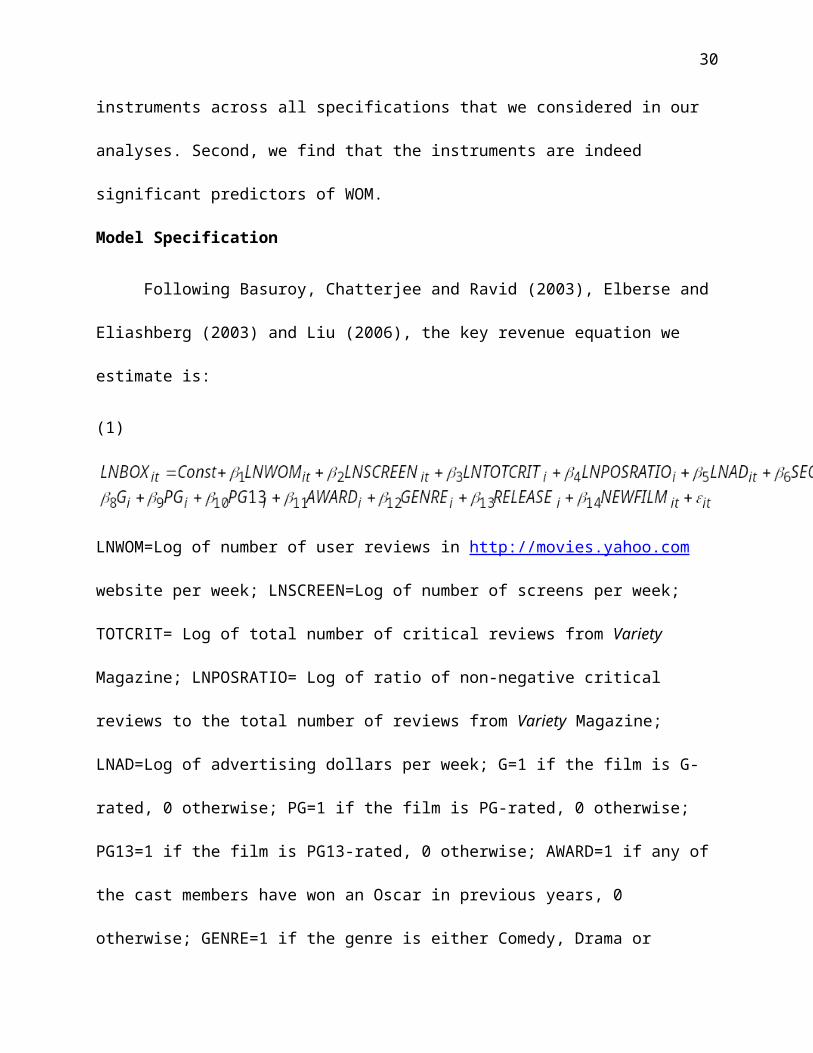
Model Specification

Following Basuroy, Chatterjee and Ravid (2003), Elberse and Eliashberg (2003) and Liu

(2006), the key revenue equation we estimate is:

19

(1)

LNWOM=Log of number of user reviews in http://movies.yahoo.com website per week;

LNSCREEN=Log of number of screens per week; TOTCRIT= Log of total number of critical

reviews from Variety Magazine; LNPOSRATIO= Log of ratio of non-negative critical reviews to

the total number of reviews from Variety Magazine; LNAD=Log of advertising dollars per week;

G=1 if the film is G-rated, 0 otherwise; PG=1 if the film is PG-rated, 0 otherwise; PG13=1 if the

film is PG13-rated, 0 otherwise; AWARD=1 if any of the cast members have won an Oscar in

previous years, 0 otherwise; GENRE=1 if the genre is either Comedy, Drama or Action, 0

otherwise; RELEASE=1 if the release date is the weekend of Memorial Day, July 4,

Thanksgiving or Christmas and 0 otherwise; NEWFILM=Number of new films in the Top 20 per

week. Week fixed effects are captured using weekly dummies and are not shown in the equation.

The log transformations have been accomplished by adding 1 to the value of the variable.

First, we replicate prior work using WOM as an exogenous variable using OLS. We

expect that its impact on revenues will be positive and significant. The results of nested models

– Model 1, Model 2 and Model 3 presented in Table 4 confirm our expectations. The findings

replicate prior research (Chevalier and Mayzlin 2006; Liu 2006; Zhu and Zhang 2010). The

coefficient of WOM is positive and significant in each of these three nested models.

----------------------------------------Insert Table 4 Here

----------------------------------------

Models 4 and 5 are fixed effects regressions. In both of these regressions, the coefficient of

WOM is positive and significant. In addition, we also run a regression of the first differences to

contrast our results with those of Chevalier and Mayzlin (2006) and Zhu and Zhang (2010) who

20

run such difference models. The coefficient of WOM in Model 6 is still positive and significant.

However, from Levitt’s seminal papers (1996 and 1997) and from papers by other authors who

have tackled endogeneity issues, we know that difference equations may not solve the

endogeneity issue, and hence, we run IV regressions next.

Instrumental variables regressions and tests

Now we consider the scenario where both WOM and screens are endogenous.

Consequently, we run a series of instrumental variable regressions. As noted, we conduct several

additional statistical tests to determine the relevance (correlation with the endogenous variables)

and validity (orthogonality of the residuals or exogeneity with the dependent variable) of these

instrumental variables. Overall we find that our instruments satisfy the relevance and exogeneity

criteria necessary for valid instruments. We describe these tests in detail below.

In all the tests that we report, two issues are important. The first is the issue of

heteroskedasticity. In the context of IV estimation (2SLS) heteroskedasticity does not cause bias

or inconsistency in the estimators (Bascle 2008; Stock and Watson 2008). However, the standard

errors and test statistics come into question even with large sample sizes (Wooldridge 2003).

Thus heteroskedasticity prevents valid inferences. Hence, we control for heteroskedasticity in all

our estimations by using heteroskedasticity adjusted White’s robust standard errors. The second

is the issue of serial correlation. Like heteroskedasticity, in the presence of serial correlation,

standard errors and test statistics are not valid. This is especially critical for cross-sectional time

series panel data such as ours and those used in Liu (2006) and Zhu and Zhang (2010). Hence we

control for serial correlation in two ways. First, we use week fixed effects to control for weekly

variations (see Oberholzer-Gee and Strumpf 2007). Second, we use a lag selection procedure of

Newey-West (1994) in the estimations. Note that with these two issues taken care of, our

21

resulting statistics are now robust to both heteroskedasticity and autocorrelation or as

econometricians say: ‘heteroskedasticity-and autocorrelation-consistent’ (HAC). Lastly, since we

have a number of non time varying movie-specific variables, such as genre, rating, etc., by

including them in these regressions we control for movie-fixed effects. In addition, Stock Wright

and Yogo (2002) and others (e.g., Stock 2001; Yogo 2004) recommend that the 2SLS estimation

should be performed with the generalized method of moments procedure (GMM) in the presence

of heteroskedasticiy and serial correlation to allow for efficient estimations when the model is

over-identified. Therefore, our estimations use GMM (see Chintagunta, Gopinath and

Venkataraman 2009).

Table 5 presents the results of estimations of the 2SLS specifications using GMM. We

run two nested models – Model 1 is nested in Model 2. In the first two columns of Model 1 and

Model 2 we report the results of the first stage of the 2SLS specifications of the two endogenous

variables. The key statistics related to endogeneity and instrumental variable selection appear in

the bottom panel of the table.

-------------------------------------------- Insert Tables 5, 6, and 7 Here--------------------------------------------

A robust and conservative test that is usually reported for instrument relevance is the first-stage

F-statistic developed by Stock and Yogo (2004). This is an F-statistic that tests whether the

coefficients on the instruments are equal to zero in the structural equation. Stock and Yogo

(2004: Table 1) report that when there is one endogenous regressor, the first-stage F-statistic of

the 2SLS regression should have a value of 10 or higher. When one exceeds this threshold of

Stock and Yogo (2004), one can be reasonably certain that the instruments are strong, i.e., they

satisfy the relevance condition. In Table 5, for Model 1 the F values are 33.87 and 16.68, while

22

for Model 2 they are 29.16 and 13.81 respectively. The Shea partial R-square values and the F-

statistic provide significant support for the joint relevance of all our instruments. Further, the

Anderson-Rubin F-statistic rejects the null hypothesis and indicates that the endogenous

regressors are indeed relevant. Now we turn to the tests of instrument exogeneity.

The exogeneity condition, which is also known as the orthogonality condition, implies

that the instruments should not be correlated with the error term of the structural equation.

Exogeneity tests require us to have more instruments than the endogenous regressors and for the

equation to be over-identified. Over-identification is appealing because it helps us to not only

investigate the exogeneity of the instruments but also to ensure better finite sample properties for

the IV estimators (Davidson and MacKinnon 1993). One of the key tests for exogeneity is

Sargan or Hansen’s J-statistic which has a Chi-square distribution with m-k degrees of freedom

(m=# of instruments, k=# of endogenous variables). It tests whether the instruments are

exogenous. The Hansen’s J-statiastic is robust to heteroskedasticity. In Table 5, this J-statistic

reported in column 3 for Model 1 is 6.908 with a p-value of .141 and in column 6 for Model 2 it

is 6.482 with a p-value of .166. Thus in both cases the Hansen’s J-statistic is unable to reject the

null hypothesis that the instruments are valid and orthogonal to the residuals, and their exclusion

from the main estimated equation is appropriate.

However, Hansen’s J-statistic usually assumes that at least one instrument is exogenous.

Hence if none of the instruments is exogenous, the J-statistic will be biased and inconsistent and

may even erroneously fail to reject the null hypothesis (Murray 2006a). This potential problem is

addressed with the difference-in-Sargan statistic, which can be only used if we have at least two

more instruments than endogenous regressors. This statistic is commonly referred to as the C-

statistic; it is the difference between two J-statistics and tests the exogeneity of one or more

23

instruments by relying on one other or several other instruments that are assumed to be

exogenous (Baum, Schaffer and Stillman 2003). We specifically checked the exogeneity of the

key instrument, WOM_BUDGET and the C-statistic reported in Table 5 for Model 1 (column 3)

is .418 with a p-value of .518 while that for Model 2 (column 6) is .357 with a p-value of .549.

Thus for both models we find that this instrument can be considered as exogenous given that the

null hypothesis is not rejected at the 10 percent level. All tests also show that the exogeneity of

the instruments that we use is respected.

Several econometricians (Andrews, Moreira and Stock 2006 and 2007; Moreira 2003)

recommend to compare the instrumental variables results to those obtained by a method called

Moreira’s conditional likelihood ratio (Moreira’s CLR). A key advantage of this method is that it

draws correct inferences independent of the strength of the instruments. Andrews, Moreira and

Stock (2006) show that Moreira’s CLR is the most powerful test when the model is either exactly

identified or over-identified and the resulting confidence intervals are nearly optimal. Therefore

we run Moreira’s CLR test for endogenous WOM, and we obtain a confidence interval of

[-.036852, .0990235] with a p-value of .38 which is not significant. Thus Moreira’s CLR is

unable to reject the null hypotheses that the coefficient of WOM is zero, providing a strong

support for the results in Table 5 and our general conclusion of insignificance of WOM.

Murray (2006b) states that “If the parameter estimates using different instruments

differ appreciably and seemingly significantly from one another, the validity of the instruments

becomes suspect” (p. 15). Therefore, we create another set of alternative instruments for WOM:

the number of WOM of all other movies within the same MPAA rating class (WOM_RATING),

its square term (WOM_RATINGSQ) and WOM_RATINGAGE by interacting WOM_RATING

24

variable with the average age of movies every week. The various tests uphold both the validity

and the exogeneity of these instruments as well.

In conclusion, our results support the idea that WOM does not affect revenues,

supporting Hypothesis 1. At the same time, we find that the ratio of non-negative reviews to total

reviews increases revenues. The total number of critical reviews also increases revenues. Both of

these results support hypothesis 2. In other words, our findings seem to indicate that whereas the

volume of WOM co-moves with revenues and does not affect the success of motion pictures,

professional reviews seem to determine revenues as shown supporting other work (see Basuroy,

Chatterjee and Ravid 2003; Elberse and Eliashberg 2003; Eliashberg and Shugan 1997; Ravid

1999 and others). Next we turn to dynamic instrumental variable analyses.

Dynamic Instrumental Variable Analysis.

The model in equation 1 and the results reported in Table 5 allow only for a

contemporaneous effect of WOM on revenues. But it is quite possible that endogenous variables

influence box office revenues at a later point in time. In Table 6 we address this issue by

studying the effect of lagged endogenous variables, weighted stocks of endogenous variables,

and lagged and weighted stock of advertising on revenues5. Table 6 reports the second-stage

results but includes all relevant statistics from the first-stage regressions.

Model 1 in table 6 uses lagged WOM and screens but current advertising. Model 2 uses

current WOM and screens, but lagged advertising. Model 3 uses current WOM, lagged screens

and weighted stock of current and previous period’s advertising (current week is weighted .66

while previous week is weighted .34). Model 4 uses lagged weighted stock of advertisement.

Model 5 uses weighted stock of current and previous week’s WOM and advertising (current

5 We thank the Associate Editor and an anonymous referee for the suggestion to analyze stock values of WOM and AD.

25

week is weighted .66 while previous week is weighted .34) and lagged screens. This formulation

tests extensively for the possibility that past and/or current WOM affect current revenues.

The results are all consistent and similar to each other and also consistent with results reported in

Table 5: the coefficient of WOM is insignificant and the coefficients of the professional critical

reviews variables are significant as in our previous table. In summary, all our 2SLS estimates

with various nested models, whether dynamic or current, using different sets of instruments,

controlling for heteroskedasticity and serial correlations with movie-fixed effects using GMM

procedure show the same basic result: the coefficient of WOM is not significant once we take its

endogeneity into account and instrument for it, whereas professional reviews seem to determine

box office success. Thus we find strong support for H1 and H2.

At this point it is important to evaluate whether these instrumental variable estimates are

superior to OLS estimates. Hahn and Hausman (2005) show that the ratio between the finite-

sample bias of two-stage least squares and ordinary least squares is given by:

(Murray 2006a, p. 124) where n is sample size, 2 is the R-square of the first stage, and l is the

number of instruments. The results and numbers in Table 5, show that the biases of our IV

estimations are significantly less than those of the OLS. Our results, therefore, conclusively show

that the IV estimates are superior to the OLS estimates.

Hypothesis 3 states that WOM increases with the dispersion of critical reviews but may

decrease as dispersion becomes extreme. Testing interaction of endogenous variables warrants

special caution. Since WOM is endogenous, any interaction term such as WOM*CRITDISP

being a function of the endogenous variable, is also endogenous and hence needs additional

instruments for proper estimation which we use (see, Wooldridge 2003, p. 515 for details on

26

implications of interaction terms of endogenous variables). This is a critical fact that is often

overlooked. Hence we use additional instruments to account for this. Results are reported in

Model 1 in Table 7. The coefficient of the interaction term, WOM*CRITDISP is positive and

significant while that of the WOM*CRITDISP_SQ is negative and significant. Thus it appears

that the impact of WOM on revenues grows with higher levels of dispersion of professional

critical reviews, but at a decreasing rate. Thus we find support for H3. Another simple way of

understanding this finding is to suggest that critics generally are more important than WOM, but

when critics are split, WOM is considered a viable source of information.

Hypothesis 4 proposes that for platform release movies, WOM will play a significant role

in affecting box office revenues. Once again, note that this test requires an interaction term with

the endogenous variable, and hence we use additional instruments for this test. Model 2 in Table

7 reports the results. While the coefficient of WOM remains insignificant, the interaction of

WOM and platform release dummy is negative and significant, and hence, does not support H4.

For platform release movies, the mean WOM is 15.62, close to one-fifth of the overall mean of

WOM in Table 2 (68.59). Thus, platform-release movies generate significantly less WOM and

WOM exerts negative impact on box office revenues contrary to expectations. However, note

that professional reviews still significantly determine the outcome. A possible interpretation is

that for movies which may be controversial or experimental, professional views help put the

movie going experience in perspective, whereas internet WOM may carry negative views.

Discussion, Managerial Implications and Conclusion

Marketing practitioners and scholars are paying significant attention to word-of-mouth.

WOM communication in the form of online product reviews and commentaries has become a

major source of information for consumers. The phrase “word of mouth” returns 22 million hits

27

on Google. Amazon lists many practitioner books on the subject with evocative titles such as

Word of Mouth Marketing: How Smart Companies get people Talking, Word of Mouth: A Guide

to Commercial Voice-over Excellence, and others. There is also a Word Of Mouth Marketing

Association (www.womma.org) that claims itself to be “the leading trade association in the

marketing and advertising industries that focuses on word of mouth …” The general

understanding from practitioners’ perspective is that WOM’s effect on sales and revenues is

positive and significant (as documented by case studies or stories). The topic has garnered active

interest amongst scholars, and as a result, numerous academic papers have been published in the

marketing area as well as in other areas such as management, economics, finance, etc. In most

marketing studies that we are aware of, this variable is treated as an exogenous variable

(Chevalier and Mayzlin 2006; Liu 2006; Sun 2009; Zhu and Zhang 2010). Our paper is perhaps

one of the first in this area to point out that practitioners as well as academics may be

overemphasizing and overestimating the true effect of WOM.

Our first result is that if the volume of internet WOM is treated as an exogenous variable,

it will exhibit significant positive impact on revenues, confirming prior research. But omitted

variable bias requires treating WOM as an endogenous variable, and IV regressions with proper

instruments show WOM has no significant impact on box office revenues. WOM does co-move

with revenues, but as we show, does not determine the outcome. The key take-away from this

result is that managers have to be cautious regarding their reliance on WOM. The rosy picture

painted by popular media regarding the ubiquitous positive impacts of WOM has to be taken

with a grain of salt.

The growth of online WOM is increasingly challenging the importance of professional

critics. However, contrary to this commonly accepted sentiment, both in academia and in the

28

trade press, our second result suggests that professional critics are significant predictors of

revenues even in the face of WOM (this complements earlier work on the value of critical

reviews in the absence of WOM). Our findings seem rather intuitive- would you buy a computer

based upon a review of a professional, or would you prefer an opinion posted on the internet by

Joe Shmoe from Nowhereland USA? While the movie going experience is different than a

consumption good, our findings suggest that an element of expertise is important. This perhaps

explains the cozy relationships studios still maintain with critics and the existence of blurbs from

critics which are an integral part of most movie advertisements. Our findings therefore reinforce

this aspect and suggest that studios need to carefully integrate critical reviews and WOM in the

promotional efforts. Despite media reports of waning effects of professional critics (Babej and

Pollack 2006), our findings show that efforts to cut out critics and solely relying on word-of-

mouth may not be the best idea for studios. We believe that studios are aware of this fact judging

by the prominent place of blurbs, and reviewer affiliations that appear prominently in various

advertisements.

Our third result shows that volume of WOM may be significant when professional critics

disagree, and therefore, controversial movies may gain from WOM. Therefore, studios may want

to encourage WOM for movies that earned split reviews. However, only moderate level of

controversy or critical dispersion is optimal. Studios are known to spin negative opinions in a

more positive light, and that may be a viable option to balance the proportion of negative reviews

for WOM to kick in.

Our fourth result shows that the conventional wisdom that platform release strategy

creates WOM necessary for movie success, may not be true. We do not find any significant

impact of WOM on box office revenues for platform release movies. However, professional

29

reviews seem to matter a great deal. Thus, professional critical reviews should be taken even

more seriously if a platform release is planned and if reviews turn out not to be great, the studio

may expect a bad run.

We conclude that studios may benefit from trying to manage or at least influence WOM

on the internet. However, the intricate nature of the interactions of WOM suggests that this is a

very challenging and delicate task.

30

References

Andrews, D. W. K., M. J. Moreira, J. H. Stock. (2006). Optimal Two-Sided Invariant Similar Tests for Instrumental Variables Regression. Econometrica 74(3): 715–52.

----, ---- , ---- . 2007. Performance of Conditional Wald Tests in IV Regression with Weak Instruments. Journal of Econometrics 139(1): 116–32.

Angrist, J. D., A. B. Krueger. 2001. Instrumental Variables and the Search for Identification: From Supply and Demand to Natural Experiments. Journal of Economic Perspectives, Vol. 15 (4), 69-85.

Bascle, G. 2008. Controlling for endogeneity with instrumental variables in strategic management research. Strategic Organization Vol. 6 (3) 285-327.

Basuroy, S., S. Chatterjee, S. A. Ravid. 2003. How Critical Are Critical Reviews? The Box Office Effects of Film Critics, Star Power, and Budgets. Journal of Marketing 67 (October) 103–117.

----, K. K. Desai, D. Talukdar. 2006. An Empirical Investigation of Signaling in the Motion Picture Industry. Journal of Marketing Research 43, 2, 287-295.

Baum, C. F., M. E. Schaffer, S. Stillman. 2003. Instrumental Variables and GMM: Estimation and Testing. Stata Journal 3(1): 1–31.

Berlyne, D. E.1971. Aesthetics and Psychobiology, New York: Meredith.

Bughin, J., J. Doogan, O. J. Vetvik. 2010. A new way to measure word-of-mouth marketing. McKinsey Quarterly (April).

Brown, J., P. Reingen. 1987. Social Ties and Word-of-Mouth Referral Behavior. Journal of Consumer Research, 14 (December), 350–62.

Caves, R. E. 2000. Creative industries: Contracts Between Art and Commerce. Cambridge, Mass.: Harvard University Press.

Chaffee, S.1982. Mass Media and Interpersonal Channels: Competitive, Convergent, or Complementary?” in Inter/Media: Interpersonal Communication in a Media World, Gary Gumpert and Robert Cathcart, eds. New York: Oxford University Press.

Chevalier, J. A. and D. Mayzlin. 2006. The Effect of Word of Mouth on Sales: Online Book Reviews. Journal of Marketing Research, Vol. XLIII (August 2006), 345–354.

Chisholm, D. C. 2000. The war of attrition and optimal timing of motion pictures release.Working paper, Suffolk University, Department of Economics.

31

Chintagunta, P. K., S. Gopinath, S. Venkataraman. 2009. Online word-of-mouth effects on the offline sales of sequentially released new products: An application to the movie market. Working paper. University of Chicago.

Clemons, E. K., G. Gao, L. M. Hitt. 2006. When Online Reviews Meet Hyperdifferentiation: A Case Study of the Craft Beer Industry. Journal of Management Information Systems, Vol. 23, No. 2 (Fall), 149-171.

Crowley, A. E., W. D. Hoyer. 1994. An Integrative Framework for Understanding Two-Sided Persuasion. Journal of Consumer Research, Vol. 20, No. 4 (March), 561-574.

Davidson, R., J.G. MacKinnon. 1993. Estimation and Inference in Econometrics, Oxford Economic Press: Oxford, UK.

Dellarocas, C., R. Narayan. 2006. A Statistical Measure of a Population’s Propensity to Engage in Post-Purchase Online Word-of-Mouth. Statistical Science, 2006, Vol. 21, No. 2, 277–285.

----, N. Awad, M. Zhang. 2004. Exploring the Value of Online Reviews to Organizations: Implications for Revenue Forecasting and Planning. Working paper, MIT Sloan School of Management.

Desai, K. K., and S. Basuroy. 2005. Interactive Influences of Genre FGamiliarity, Star Power, and Critics’ Reviews In the Cultural Goods Industry: The Case of Motion Pictures. In Psychology and Marketing, 22 (3), 203-223.

DeVany, A., D. Walls. 2002. Does Hollywood Make Too Many R-Rated Movies? Risk, Stochastic Dominance, and the Illusion of Expectation. Journal of Business, 75 (3), 425–451.

Einav, L. 2007. Seasonality in the U.S. motion picture industry. Rand Journal of Economics, Vol. 38, No. 1 (Spring), 127-145.

Elberse, A., J. Eliashberg. 2003. Demand and Supply Dynamics Behavior for Sequentially Released Products in International Markets: The Case of Motion Pictures. Marketing Science, 22 (3), 329-354.

Eliashberg, J. and Steven. M. Shugan (1997), “Film Critics: Influencers or Predictors?” Journal of Marketing, Vol. 61, (April), 68-78.

Faber, R., T. O’Guinn. 1984. Effect of Media Advertising and Other Sources on Movie Selection. Journalism Quarterly, 61, 371–77.

Godes, D. and D. Mayzlin. 2004. Using Online Conversations to Study Word-of-Mouth Communication. Marketing Science, 23 (4), 545–60.

32

Golden, L. L., M. I. Alpert. 1987. Comparative Analyses of the Relative Effectiveness of One-sided and Two-sided Communications for Contrasting Products. Journal of Advertising, 16 (1), 18-28.

Goh, J. C., L. H. Ederington. 1993. Is a Bond Rating Downgrade Bad News, Good News, or No News for Stockholders. Journal of Finance, 48 (5), 2001-08.

Greco, A. N. 1997. The Book Publishing Industry. Allyn Bacon, Needham Heights: MA.

Hahn, J., J. Hausman. 2005. Instrumental Variable Estimation with Valid andInvalid Instruments. Working paper, MIT, Cambridge, MA.

Harrison-Walker, L. J. 2001. The Measurement of Word-of-Mouth Communication and an Investigation of Service Quality and Customer Commitment as Potential Antecedents. Journal of Services Marketing, 4 (1), 60–75.

Hennig-Thurau, T., M. B. Houston, G. Walsh. 2006. The Differing Roles of Success Drivers Across Sequential Channels: An Application to the Motion Picture Industry. Journal of the Academy of Marketing Science, 34, No. 4, 559-575.

----, ----, and S. Sridhar. 2006. Can good marketing carry a bad product? Evidence from the motion picture industry. Marketing Letters, Vol. 17, No. 3, 205-219.

----, ----, T. Heitjans. 2009. Conceptualizing and Measuring the Monetary Value of Brand Extensions: The Case of Motion Pictures. Journal of Marketing, Vol. 73 (November), 167-183.

Ho, J., T. Dhar, C. B. Weinberg. 2009. Playoff-Payoff: Superbowl Advertising for Movies. International Journal of Research in Marketing, Vol. 26 No. 3 (September) 168-179.

Holbrook, M. B. 1999. Popular Appeal versus Expert Judgements of Motion Pictures. Journal of Consumer Research, Vol. 26 (September), 144-155.

----. 2005. The Role of Ordinary Evaluations in the Market for Popular Culture: Do Consumers Have ‘Good Taste’? Marketing Letters, 16 (2, April), 75-86.

----, M. Addis. 2007. Taste versus the Market: An Extension of Research on the Consumption of Popular Culture. Journal of Consumer Research, 34 (October), 415-424.

Kale, J. R., E. Reis, A. Venkateswaran. 2009. Rank Order Tournament and Incentive Alignment: The Effect on Firm Performance. Journal of Finance 64, 1479-1512.

Kamakura, W. A., S. Basuroy, P. Boatwright. 2006. Is Silence Golden? An Inquiry Into the Meaning of Silence in Professional Product Evaluations. Quantitative Marketing and Economics, Vol. 4, No. 2, 119-141.

Levitt, S. D. 1996. The Effect of Prison Population Size on Crime Rates: Evidence from

33

Prison Overcrowding Litigation. Quarterly Journal of Economics, Vol. 111 (2), pp. 319-51.

----. 1997. Using Electoral Cycles in Police Hiring to Estimate the Effect of Policeon Crime. American Economic Review, Vol. 87(4), pp. 270-90.

Liu, Y. 2006. Word-of-Mouth for Movies: Its Dynamics and Impact on Box Office Revenue. Journal of Marketing, 70 (3), 74-89.

McGuire, W. J. 1961. The Effectiveness of Supportive and Refutational Defenses in Immunizing and Restoring Beliefs against Persuasion. Sociometry, 24 (June), 184- 197.

----. 1985. Attitudes and Attitude Change. Handbook of Social Psychology, ed. Gardner Lindzey and Elliot Aronson, Reading, MA: Addison-Wesley, 233-346.

Moreira, M. J. 2003. A Conditional Likelihood Ratio Test for Structural Models. Econometrica, 71(4): 1027–48.

Murray, M. P. 2006a. Avoiding Invalid Instruments and Coping with Weak Instruments. The Journal of Economic Perspectives, Vol. 20, No. 4 (Fall), pp. 111-132.

----. 2006b. The Bad, the Weak, and the Ugly: Avoiding the Pitfalls of Instrumental Variables Estimation. Social Science Research Network Working Paper No. 843185.

Nair, H., P. Chintagunta, J-P. Dubé. 2004. Empirical Analysis of Indirect Network Effects in the Market for Personal Digital Assistants. Quantitative Marketing and Economics, 2 (1), 23–58.

Neelamegham, R., P. Chintagunta. 1999. A Bayesian Model to Forecast New Product Performance in Domestic and International Markets. Marketing Science, 18 (2), 115–36.

Newey, W. K. and K.D. West. 1994. Automatic Lag Selection in Covariance MatrixEstimation. Review of Economic Studies 61(4): 631–53.

Oberholzer-Gee, F., K. Strumpf. 2007. The Effect of File Sharing on Record Sales: An Empirical Analysis. Journal of Political Economy, No. 1, Vol. 115, 1-42.

Palia, D. 2001. The Endogeneity of Managerial Compensation in Firm Valuation: A Solution. The Review of Financial Studies, Vol. 14 (Fall), No. 3, pp. 735-764.

Ravid, S. A. 1999. Information, Blockbusters, and Stars: A study of the Film Industry. Journal of Business, Vol. 72, No. 4, (October), 463-92.

----, S. Basuroy. 2004. Managerial Objectives, the R-rating Puzzle, and the Production of Violent Films. Journal of Business, Vol. 77, No. 2, S155-S192.

34

----, J.K. Wald, S. Basuroy. 2006. Distributors and critics: it takes two to tango?” Journal of Cultural Economics, 30, pp. 201-218.

Rogers, E. 1983. Diffusion of Innovations. New York: The Free Press.

Schiffman, L. G., L. L. Kanuk. 1995. Consumer Behavior, 9th Ed. Upper Saddle River, NJ: Prentice Hall.

Stock, J. H. 2001. Instrumental Variables in Statistics and Economics. InternationalEncyclopedia of the Social and Behavioral Sciences, 7577–82.

----, M. W. Watson. 2007. Introduction to Econometrics, 2nd Edition, Pearson-Addison Wesley: Boston, MA.

----, M. Yogo. 2004. Testing for Weak Instruments in Linear IV Regression.Working Paper, Department of Economics, Harvard University, Cambridge, MA.

----, J. H. Wright, M. Yogo. 2002. A Survey of Weak Instruments and Weak Identification in Generalized Method of Moments. Journal of Business and Economic Statistics, 20:4, pp. 518-29.

Sun, M. 2009. How Does Variance of Product Ratings Matter? Graduate School of Business, Stanford University, Working Paper.

Vogel, H. L. 2001. Entertainment Industry Economics, 5th ed. Cambridge, UK: Cambridge University Press.

West, P. M., S. M. Broniarczyk. 1998. Integrating Multiple Opinions: The Role of Aspiration Level on Consumer Response to Critic Consensus. Journal of Consumer Research, Vol. 25 (June), 38-51.

Wooldridge, J. M. 2003. Introductory Econometrics: A Modern Approach, 2nd edition, Thomson-Southwestern.

Yogo, M. 2004. Estimating the Elasticity of Intertemporal Substitution When Instruments are Weak. The Review of Economics and Statistics 86(3): 797–810.

Zhu, F., X. Zhang. 2009. Impact of Online Consumer Reviews on Sales: The Moderating Role of Product and Consumer Characteristics. Journal of Marketing,Vol. 74, Number 2, (March), 133-148.

35

FIGURE 1. CONCEPTUAL FRAMEWORK

THE HYPOTHESIZED ROLE OF WORD-OF-MOUTH IMPACTING

BOX OFFICE REVENUES

WOM Box Office Revenues

Critical Reviews

Dispersion of Critical Reviews

Platform Release Strategy

H1

H3H4

H2

36

0

1000

2000

3000

4000

5000

6000

7000

1 2 3 4 5 6 7 8

Box

Off

ice &

Use

r Rev

iew

s

Week

Figure 2 A. Box Office and User Reviews of Fahrenheit 9/11Released June 23, 2004

Domestic Total Gross: $119.194 million

Number of User Reviews

Box Office Revenue (10 thousands)

0

500

1000

1500

2000

2500

3000

3500

4000

4500

1 2 3 4 5 6 7 8

Box

Off

ice

& U

ser

Rev

iew

s

Week

Figure 2 B. Box Office and User Reviews of Spider-Man 2Released June 30, 2004

Domestic Total Gross: $373.6 million

Number of User Reviews

Box Office Revenue (10 thousands)

37

TABLE 1: List of Variables Used in the Analysis, Their Definitions, References, and SourcesVariables Variable Definition Literature Support Data Source

BOXit Box office revenue of film i in week t (in regressions we use natural log). Add 1 for log transform

Basuroy, Chatterjee and Ravid (2003; Liu (2006)

Baseline

WOMit Number of user comments for film i in week t (in regressions we use natural log). Add 1 for log transform

Dellarocas et al (2007); Sun (2009); Liu (2006); Chintagunta et al. (2009)

http://movies.yahoo.com

SCREENit The number of screens for film i in week t (in regressions we use natural log). Add 1 for log transform

Basuroy, Chatterjee and Ravid (2003); Liu (2006)

Baseline

TOTCRITi Total number of professional critical reviews (pro+con+mixed) from Variety magazine for film i

Basuroy, Chatterjee and Ravid (2003); Liu (2006);

Variety Magazine

POSRATIOi Ratio of Non-negative critical reviews for film i Ravid (1999) Variety Magazine

Gi G=1 if the film is G-rated, 0 otherwise Ravid (1999); Baseline

PGi PG=1 if the film is PG-rated, 0 otherwise Ravid (1999); Liu (2006) Baseline

PG13i PG13=1 if the film is PG13-rated, 0 otherwise Ravid (1999); Liu (2006); Baseline

AWARDi AWARD=1 if any of the cast members have won an Oscar in previous years, 0 otherwise

Basuroy, Chatterjee and Ravid (2003); Ravid(1999)

www.imdb.com

GENREi GENRE=1 if the genre is either Comedy, Drama or Action, 0 otherwise

Desai and Basuroy (2005); Liu (2006)

Baseline

RELEASEi RELEASE=1 if the release date is the weekend of Memorial Day, July 4, Thanksgiving or Christmas

Chisholm (2000); Einav (2007); Sun (2009)

Baseline

NEWFILMit Number of new films in the Top 20 per week Elberse and Eliashberg (2003); Liu (2006)

www.boxofficemojo.com

ADit Advertising dollars per week in ‘000 (in regressions we use natural log). Add 1 for log transform

Basuroy, Desai and Talukdar (2006); Ho, Dhar and Weinberg (2009)

TNS media

CRITDISPi Dispersion of Critical Reviews=Ratio of standard deviation to the mean of the critical reviews

Sun (2009); Zhu and Zhang (2010)

Variety Magazine

PLATFORMi PLATFORM=1 if the film is released in less than 500 screens, 0 otherwise

Einav (2007) www.boxofficemojo.com ;www.imdb.com

AVGAGEit Average age of films in weeks in the Top 20 per week Elberse and Eliashberg (2003); Liu (2006)

www.boxofficemojo.com

Instrumental VariablesWOM_BUDGETit Instrumental variable: WOM per week of all other

movies whose budget is within 10% of movie iZhu and Zhang (2010); Chintagunta et al. (2009)

www.boxofficemojo.com ;www.imdb.com

WOM_BUDGETSQit Instrumental variable: Square of Zhu and Zhang (2010); Chintagunta et al. (2009)

www.boxofficemojo.com ;www.imdb.com

WOM_BUDGETAGEit Instrumental variable: Interaction of

and

Zhu and Zhang (2010); www.boxofficemojo.com ;www.imdb.com

SCREEN_RATINGit Instrumental variable: Screens per week of all other movies that has same rating as movie i

Zhu and Zhang (2010); Nair, Chintagunta et al. (2009)

Baseline;www.boxofficemojo.com

SCREEN_RATINGAGEit Instrumental variable: Interaction of

and

Zhu and Zhang (2010);Chintagunta et al. (2009)

www.boxofficemojo.com ;www.imdb.com

MAJORi Major=1 if the distributor is a major studio, 0 otherwise

Elberse and Eliashberg (2003)

Baseline

38

TABLE 2: Descriptive StatisticsN Mean SD Min Max

Box Office Revenues 1562 5290984 1.38e+07 789 2.11e+08

Word-of-Mouth: 1672 68.58 243.25 0 4768

Screens: 1562 967.95 1148.47 1 4223

Total Critical Reviews: 1881 12.20 1.73 1 21

Ratio of Non-Negative Reviews: POSRATIOi

1859 .73 .24 0 1

G-Rated Films: 1881 .01 .11 0 1

PG-Rated Films: 1881 .13 .34 0 1

PG13-Rated Films: 1881 .37 .48 0 1

Awards Won: 1881 .33 .47 0 1

Genre: 1881 .70 .73 0 1

Release: 1881 .13 .34 0 1

New Films: 1649 3.04 1.12 1 6

Advertising: 1881 1527.38 4384.86 0 32554.3

Dispersion of Critical reviews: 1859 .60 .40 .11 2.34

1672 5.49 3.52 2.9 26.2

1009 155.07 423.15 0 7613

1009 202925.5 2021200 0 5.80e+07

1009 753.30 2208.04 0 39587.6

1575 11197.9 5710.65 88 27151

1575 63301.93 60409.9 409.05 467172.2

1881 .53 .50 0 1

WOM=Number of posts in movies.yahoo.com website per week; SCREEN=Number of screens per week; TOTCRIT= Total number of critical reviews from Variety Magazine; POSRATIO=Ratio of non-negative critical reviews; G=1 if the film is G-rated, 0 otherwise; PG=1 if the film is PG-rated, 0 otherwise; PG13=1 if the film is PG13-rated, 0 otherwise; AWARD=1 if any of the cast members have won an Oscar in previous years, 0 otherwise; GENRE=1 if the genre is either Comedy, Drama or Action, 0 otherwise; RELEASE=1 if the release date is the weekend of Memorial Day, July 4, Thanksgiving or Christmas; NEWFILM=Number of new films in the Top 20 per week; AD=Advertising dollars per week in ‘000; CRITDISP=Ratio of standard deviation to the mean of the critical reviews; AVGAGE=average age in weeks of top 20 films; WOM_BUDGET=WOM per week of all other movies that have similar budget within + or – 10%; WOM_BUDGETSQ=Square of WOM_BUDGET; WOM_BUDGETAGE=Interaction of WOM _BUDGET and AVGAGE; SCREEN_RATING=Number of screens of all other movies that have same mpaa rating; SCREEN_RATINGAGE=Interaction of SCREEN_RATING and AVGAGE; MAJOR=1 if the studio is a major studio (i.e. MGM, Warner Brothers, Columbia, Universal, Paramount, Buena Vista, 20th Century Fox, Dreamworks SKG), 0 otherwise

39

TABLE 3: Correlation Table1 2 3 4 5 6 7 8 9 10 11 12 13 14 15

1BOXit 1.00

2 WOMit .34 1.00

3 SCREENit.65 .32 1.00

4 TOTCRITi .23 .10 .26 1.00

5 POSRATIOi.04 .06 -.06 -.01 1.00

6 NEWFILMi -.12 -.06 -.04 -.01 -.00 1.00

7 ADit .63 .36 .61 .19 .12 -.10 1.00

8 CRITDISPi -.04 -.04 .03 -.06 -.93 -.02 -.11 1.00

9 WOM_BUDGETit .06 .19 .11 .03 -.01 -.07 .05 -.01 1.00

10 WOM_BUDGETSQit .08 .14 .09 .02 .03 -.06 .06 -.03 .81 1.00

11 WOM_BUDGETAGEit .07 .23 .12 .04 -.01 -.07 .06 -.00 .86 .79 1.00

12 SCREEN_RATINGit -.09 -.04 -.10 .10 -.21 .01 -.09 .13 -.05 -.05 -.03 1.00

13 SCREEN_RATINGAGEit

-.04 .01 -.04 .07 -.14 -.08 -.07 .09 -.07 -.04 -.01 .54 1.00

14 MAJORi .11 .15 .34 .28 -.19 -.00 .22 .16 .07 .04 .08 .08 -.01 1.00

15 AVGAGEit .00 .06 .02 .03 -.04 -.12 -.03 .03 -.06 -.01 .00 .05 .79 -.04 1.00

BOX=box office revenues; WOM=Number of posts in movies.yahoo.com website per week; SCREEN=number of screens per week; TOTCRIT= Total number of critical reviews from Variety Magazine; POSRATIO=Ratio of non-negative reviews; NEWFILM=Number of new films in the Top 20 per week; AD=Log of advertising dollars per week; CRITDISP=Ratio of standard deviation to the mean of the critical reviews; WOM_BUDGET=WOM per week of all other movies that have similar budget (within + or – 10%); WOM_BUDGETSQ=Square of WOM_BUDGET; WOM_BUDGETAGE=Interaction of WOM _BUDGET and AVGAGE which is the average age in weeks of top 20 films; SCREEN_RATING=Number of screens of all other movies that have same mpaa rating; SCREEN_RATINGAGE=Interaction of SCREEN_RATING and AVGAGE which is the average age in weeks of top 20 films; MAJOR=1 if the studio is a major studio (i.e. MGM, Warner Brothers, Columbia, Universal, Paramount, Buena Vista, 20th Century Fox, Dreamworks SKG), 0 otherwise; AVGAGE=average age in weeks of top 20 films;

40

Table 4: OLS Estimations, Dependent Variable is ln (boxoffice) Model 1 Model 2 Model 3 Model 4#

(Fixed Effects) Model 5#

(Fixed Effects) Model 6§

(1st Difference)Dependent Variables LNBOXit LNBOXit LNBOXit LNBOXit LNBOXit LNBOXit

Word-of-Mouth: LNWOMit .059(.013)** .073(.013)** .017(.008)* .056(.022)** .025(.012)* .069(.022)**Screens: LNSCREENit .960(.018)** .963(.019)** .857(.015)** .700(.029)** .846(.019)** .266(.043)**Critical Reviews: LNTOTCRITi

.143(.049)** .107(.050)* .070(.038) Dropped Dropped Dropped

Ratio of Non-Negative Reviews: LNPOSRATIOi

.558(.047)** .536(.047)** .275(.037)** Dropped Dropped Dropped

Advertising: LNADit .183(.010)** .292(.009)** .070(.008)** .092(.012)**Sequel: SEQUELi .302(.081)** .120(.047)** Dropped Dropped Dropped Gi 1.048(.169)** .725(.075)** Dropped Dropped Dropped PGi -.324(.079)** -.141(.05)** Dropped Dropped Dropped PG13i -.245(.057)** -.123(.04)** Dropped Dropped Dropped Awards Won: AWARDi .066(.052) .059(.032) Dropped Dropped Dropped Genre: GENREi .016(.034) .011(.020) Dropped Dropped Dropped Release: RELEASEi .067(.071) .090(.045)* Dropped Dropped Dropped New Films: NEWFILMit -.029(.014)* -.045(.010)** -.021(.007)** -.011(.010)Constant 7.94(.101)** 8.021(.102)** 7.632(.104) 8.52(.132)** 7.81(.083)No. of Observations 1532 1532 1312 1541 1337 1108 R-square .842 .849 .939 .878 .947 .167F-value 1574.86 612.33 917.66 1441.04 998.72 34.93Prob. > F .00 .00 .00 .00 .00 .00Week Fixed Effects NO NO YES NO YES NOHeteroskedasticity YES YES YES YES YES YES** p < .01; * p < .05; White’s heteroskedasticity adjusted standard errors in parentheses;

# in a fixed effects regression, all non-time varying variables are dropped

§in a Difference equation yt - yt-1=β1 (xt - xt-1)+… all non time-varying variables are dropped. Model 6 is a First Difference equation.

LNWOM=Log of number of posts in movies.yahoo.com website per week; LNSCREEN=Log of number of screens per week; LNTOTCRIT= Log of total number of critical reviews from Variety Magazine; LNPOSRATIO=Log of ratio of non-negative reviews; LNAD=Log of advertising dollars per week; SEQUEL=1 if the film is a sequel, 0 otherwise; G, PG, PG13=1 if the film is G-rated, PG-rated or Pg13-rate respectively, 0 otherwise; AWARD=1 if any of the cast members has won an Oscar in previous years, 0 otherwise; GENRE=1 if the genre is either Comedy, Drama or Action, 0 otherwise; RELEASE=1 if the release date is the weekend of Memorial Day, July 4, Thanksgiving or Christmas; NEWFILM=Number of new films in the Top 20 per week. All log transformations have been accomplished by adding 1 to the value of the variable.

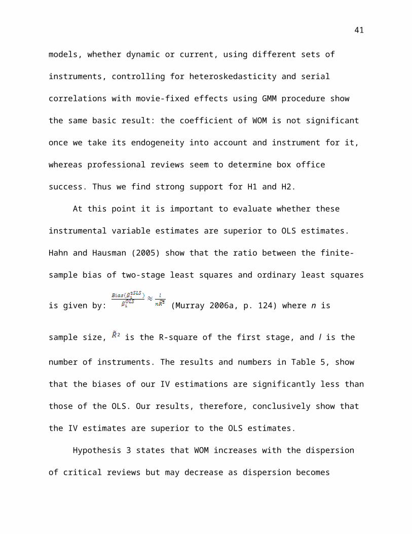
41

Table 5. Instrumental Variables Regression Results Using GMM Estimations Controlling for Serial Correlation and HeteroskedasticityModel 1 Model 2

First-Stage (1)

First-Stage (2)

Second-Stage (3)

First-Stage(4)

First-Stage(5)

Second-Stage (6)

Dependent Variables LNWOMit LNSCREENit LNBOXit LNWOMit LNSCREENit LNBOXit

Endogenous VariablesWord-of-Mouth: LNWOMit .012(.044) .062(.039)Screens: LNSCREENit .731(.083)** .707(.075)**Control VariablesCritical Reviews: LNTOTCRITi .004(.132) .650(.116)** .212(.092)* .042(.125) .619(.115)** .227(.083)**Ratio of Non-Negative Reviews: LNPOSRATIOi

-.010(.150) -.439(.083)** .029(.063) .147(.168) -.306(.089)** .151(.058)**

Advertising: LNADit .206(.026)** .259(.018)** .293(.017)** .192(.034)** .210(.024)** .208(.017)**Sequel: SEQUELi -.352(.343) .557(.112)** .358(.079)**Gi -2.737(.363)** .357(.232) .968(.199)**PGi .103(.242) .477(.137)** -.066(.082)PG13i -.185(.278) .754(.188)** -.098(.061)Awards Won: AWARDi .186(.184) .060(.101) .071(.053)Genre: GENREi -.001(.143) .164(.056)** .061(.032)Release: RELEASEi -.661(.229)** .111(.129) .089(.076)New Films: NEWFILMit .100(.063) .096(.033)** -.019(.016)

Instrumental VariablesWOM_BUDGETit .001(.001) .001(.001) .002(.000)* .001(.000)*WOM_BUDGETSQit -2.7e-07

(6.1e-08)**-7.5e-08(2.2e-08)**

-7.1e-07(2.5e-07)**

-1.8e-07(7.4e-08)**

WOM_BUDGETAGEit .000(.000) 6.3e-06(.000) .000(.000)** 1.7e-06(.000)SCREEN_RATINGAGEit -1.6e-06

(1.5e-06)1.1e-08(9.5e-07)**

-7.5e-07(1.7e-06)

-2.7e-07(6.9e-07)

SCREEN_RATINGit .000(.000)** -.000(.000)* .000(.000) -.000(.000)**

MAJORi 1.551(.188)**

1.387(.172)** 1.624(.211)** 1.077(.169)**

Constant .076(.3748) 2.572(.289)** 7.801(.24)** -.337(.418) 2.265(.315)** 7.781(.197)**No. of Observations 924 924 789 789 789Centered R-square .279 .487 .327 .561 .918Week Fixed Effects YES YES YES YES YES YESHeteroskedasticity YES YES YES YES YES YESTests for Endogeneity: Relevance and Exogeneity of InstrumentsShea Partial R-Sq .054 .053 .083 .0681st Stage F-Statistic (p-value)

33.87(.00)

16.68(.00)

29.16(.00)

13.81(.00)

Anderson-Rubin F test (p-val) 12.55(.00) 10.42(.00)Hansen-J-Statistic (p-value)

6.908(.141)

6.482(.166)

Sargan C (p-value) .418(.518) .357(.549)** p < .01; * p < .05; White’s heteroskedasticity adjusted standard errors in parentheses; LNWOM=Log of number of posts in movies.yahoo.com website per week; LNSCREEN=Log of number of screens per week; LNTOTCRIT= Log of total number of critical reviews from Variety Magazine; LNPOSRATIO=Log of ratio of non-negative reviews; LNAD=Log of advertising dollars per week; SEQUEL=1 if the film is a sequel, 0 otherwise; G, PG, PG13=1 if the film is G-rated, PG-rated or Pg13-rate respectively, 0 otherwise; AWARD=1 if any of the cast members has won an Oscar in previous years, 0 otherwise; GENRE=1 if the genre is either Comedy, Drama or Action, 0 otherwise; RELEASE=1 if the release date is the weekend of Memorial Day, July 4, Thanksgiving or Christmas; NEWFILM=Number of new films in the Top 20 per week. All log transformations have been accomplished by adding 1 to the value of the variable.WOM_BUDGET=WOM per week of all other movies that have similar budget (within + or – 10%); WOM_BUDGETSQ=Square of WOM_BUDGET; WOM_BUDGETAGE=Interaction of WOM _BUDGET and AVGAGE which is the average age in weeks of top 20 films; SCREEN_RATING=Number of screens of all other movies that have same mpaa rating; SCREEN_RATINGAGE=Interaction of SCREEN_RATING by AVGAGE which is the average age in weeks of top 20 films; MAJOR=1 if the studio is a major studio (i.e. MGM, Warner Brothers, Columbia, Universal, Paramount, Buena Vista, 20th Century Fox, Dreamworks SKG), 0 otherwise

42

Table 6. Dynamic Panel Analysis. Instrumental Variables Regression Results Using Lagged or Weighted Stock Value of Endogenous Variables Using GMM Estimations Controlling for Both Serial Correlation and Heteroskedasticity

Model 1Second-Stage

Model 2Second-Stage

Model 3Second-Stage

Model 4Second-Stage

Model 5Second-Stage

Dependent Variables LNBOXit LNBOXit LNBOXit LNBOXit LNBOXit

Endogenous VariablesWord-of-Mouth: LNWOMit .065(.041) .064(.042) .051(.042)Lagged Word-of-Mouth: LNWOMit-1 -.055(.057)Weighted Stock of Word-of-Mouth:LNWWOMit

.063(.038)

Lagged Weighted Stock of Word-of-Mouth: LNWWOMit-1

Screens: LNSCREENit .662(.084)** .645(.091)**Lagged Screens: LNSCREENit-1 .683(.093)** .526(.073)** .532(.067)**Control VariablesCritical Reviews: LNTOTCRITi .220(.111)* .272(.088)** .329(.103)** .280(.089)** .322(.101)**Ratio of Non-Negative Reviews: LNPOSRATIOi

.082(.082) .199(.063)** .147(.074)* .253(.067)** .156(.072)*

Advertising: LNADit .352(.016)**Lagged Advertising: LNADit-1 .211(.022)**Weighted Stock of Advertising: LNWADit .319(.022)** .318(.023)**Lagged Weighted Stock of Advertising: LNWADit-1

.228(.031)**

Sequel: SEQUELi .383(.082)** .418(.098)** .391(.087)** .414(.096)**Gi 1.153(.218)** 1.105(.223)** 1.163(.222)** 1.102(.207)**PGi -.064(.084) -.006(.099) -.072(.086) -.011(.098)PG13i -.112(.068) -.046(.084) -.127(.071) -.045(.084)Awards Won: AWARDi .075(.058) .070(.071) .093(.061) .068(.071)Genre: GENREi .056(.034) .052(.043) .051(.038) .047(.042)Release: RELEASEi .049(.077) .036(.093) .025(.079) .038(.093)New Films: NEWFILMit -.039(.018)* -.051(.023)* -.043(.018)* -.058(.023)**Constant 7.840(.290)** 7.859(.202)** 7.855(.211)** 8.155(.207)No. of Observations 797 789 754 789 754Centered R-square .838 .907 .856 .898 .855Week Fixed Effects YES YES YES YES YESHeteroskedasticity YES YES YES YES YESTests for Endogeneity: Relevance and Exogeneity of InstrumentsShea Partial R-Sq§ .053/.058 .083/.066 .109/.101 .085/.064 .135/.1421st Stage F-Statistic §(p-value)

31.71(.00)/15.31(.00)

28.21(.00)/13.39(.00)

26.70(.00)/14.76(.00)

27.07(.00)/13.22(.00)

24.37(.00)/15.11(.00)

Anderson-Rubin F test (p-val) 9.81(.00) 10.24(.00) 7.89(.00) 11.05(.00) 8.63(.00)Hansen-J-Statistic (p-value)

4.587(.332) 6.211(.184) 9.730(.083) 8.304(.121) 8.844(.116)

Sargan C (p-value) .265(.607) .133(.716) .644(.422) .128(.720) .008(.927)** p < .01; * p < .05; White’s heteroskedasticity adjusted standard errors in parentheses; § There are 2 first-stage regressions, hence we report two Shea Partial R-squares and two 1st stage F-stats;

LNWOM=Log of number of posts in movies.yahoo.com website per week; LNWOMt-1=Lag of Log of number of posts in movies.yahoo.com website per week; LNWWOMt-1=Lag of Log of weighted number of posts in movies.yahoo.com website per week; LNSCREEN=Log of number of screens per week; LNSCREEN t-1=Lag of Log of number of screens per week; LNTOTCRIT= Log of total number of critical reviews from Variety Magazine; LNPOSRATIO=Log of ratio of non-negative reviews; LNAD=Log of advertising dollars per week; SEQUEL=1 if the film is a sequel, 0 otherwise; G, PG, PG13=1 if the film is G-rated, PG-rated or Pg13-rate respectively, 0 otherwise; AWARD=1 if any of the cast members has won an Oscar in previous years, 0 otherwise; GENRE=1 if the genre is either Comedy, Drama or Action, 0 otherwise; RELEASE=1 if the release date is the weekend of Memorial Day, July 4, Thanksgiving or Christmas, 0 otherwise; NEWFILM=Number of new films in the Top 20 per week. All log transformations have been accomplished by adding 1 to the value of the variable.

43

Table 7. Instrumental Variables Regression Results For Testing Hypotheses 3 and 4 Using GMM Estimations Controlling for Both Serial Correlation and Heteroskedasticity

Model 1Second-Stage

Model 2Second-Stage

Dependent Variables LNBOXit LNBOXit

Endogenous VariablesWord-of-Mouth: LNWOMit .086(.039)*Screens: LNSCREENit .720(.059)** .676(.079)**Control VariablesCritical Reviews: LNTOTCRITi .086(.114) .318(.097)**Ratio of Non-Negative Reviews: LNPOSRATIOi

n/a .180(.055)**

Advertising: LNADit .213(.019)** .182(.016)**Sequel: SEQUELi .362(.090)** .367(.074)**Gi .961(.189)** 1.082(.192)**PGi -.074(.085) -.097(.078)PG13i -.156(.065)* -.144(.061)*Awards Won: AWARDi .048(.051) .067(.054)Genre: GENREi .049(.034) .090(.038)**Release: RELEASEi .208(.093)* .086(.072)New Films: NEWFILMit -.035(.017)* -.027(.017)Critic Dispersion: CRITDISP 1.723(1.596)Square of Critic Dispersion: CRITDISP_SQ 1.07(.48)**InteractionsInteraction of WOM and Critic Dispersion: WOM*CRITDISP

.449(.153)**

Interaction of WOM and Square of Critic Dispersion: WOM*CRITDISPSQ

-.476(.178)**

Interaction of WOM and Platform Release:WOM*PLATFORM

-.189(.082)*

Constant 8.766(.466)** 9.22(.243)**No. of Observations 909 909Centered R-square .888 .919Week Fixed Effects YES YESHeteroskedasticity YES YESTests for Endogeneity: Relevance and Exogeneity of InstrumentsShea Partial R-Sq§ .032/.017/.093 .066/.123/.0601st Stage F-Statistic §(p-value)

18.91(.00)/9.74(.00)/15.37(.00)

24.20(.00)/23.09(.00)/29.72(.00)

Anderson-Rubin F test (p-val) 11.30(.00) 29.84(.00)Hansen-J-Statistic (p-value)

4.357(.359)

10.01(.075)

Sargan C (p-value) .214(.643) 1.020(.313)** p < .01; * p < .05; White’s heteroskedasticity adjusted standard errors in parentheses; § There are 2 first-stage regressions, hence we report two Shea Partial R-squares and two 1st stage F-stats;n/a: due to high correlation of POSRATIO and CRITDISP we ignore LNPOSRATIO in this regression.LNWOM=Log of number of posts in movies.yahoo.com website per week; LNSCREEN=Log of number of screens per week; LNTOTCRIT= Log of total number of critical reviews from Variety Magazine; LNPOSRATIO=Log of ratio of non-negative reviews; LNAD=Log of advertising dollars per week; SEQUEL=1 if the film is a sequel, 0 otherwise; G, PG, PG13=1 if the film is G-rated, PG-rated or Pg13-rate respectively, 0 otherwise; AWARD=1 if any of the cast members has won an Oscar in previous years, 0 otherwise; GENRE=1 if the genre is either Comedy, Drama or Action, 0 otherwise; RELEASE=1 if the release date is the weekend of Memorial Day, July 4, Thanksgiving or Christmas; NEWFILM=Number of new films in the Top 20 per week; CRITDISP=ratio of standard deviation of critics rating over mean of critics’ rating; PLATFORM=1 if the film is released on 500 or less screens, 0 otherwise.All log transformations have been accomplished by adding 1 to the value of the variable.