How many bits does it take for a stimulus to be salient?

Sayed Hossein Khatoonabadi1 Nuno Vasconcelos2 Ivan V. Bajic3 Yufeng Shan4

1,3 Simon Fraser University, Burnaby, BC, Canada, skhatoon@sfu.ca, ibajic@ensc.sfu.ca2 University of California, San Diego, CA, USA, nuno@uscd.edu

4 Cisco Systems, Boxborough, MA, USA, yshan@cisco.com

Abstract

Visual saliency has been shown to depend on the unpre-dictability of the visual stimulus given its surround. Var-ious previous works have advocated the equivalence be-tween stimulus saliency and uncompressibility. We pro-pose a direct measure of this quantity, namely the numberof bits required by an optimal video compressor to encodea given video patch, and show that features derived fromthis measure are highly predictive of eye fixations. To ac-count for global saliency effects, these are embedded in aMarkov random field model. The resulting saliency mea-sure is shown to achieve state-of-the-art accuracy for theprediction of fixations, at a very low computational cost.Since most modern cameras incorporate video encoders,this paves the way for in-camera saliency estimation, whichcould be useful in a variety of computer vision applications.

1. IntroductionVisual attention mechanisms play an important role in

the ability of biological vision to quickly parse complexscenes, as well as their robustness to scene clutter. In hu-mans, attention is driven by both the visual stimuli that com-pose the scene and observer biases that derive from high-level perception. Recently, there has been substantial inter-est in the modeling of attention mechanisms in computervision. Most of these efforts have addressed the stimu-lus driven component, typically through the development ofmodels of visual saliency. While some work has attemptedto model the influence of perceptual cues in the saliencyprocess, most works have addressed what is usually definedas bottom-up or purely stimulus driven saliency. This haslong been believed to be implemented in the early stages ofvision, via the projection of the visual stimulus along thefeatures computed by the early stages of visual cortex, andto consist of a center-surround operation. In general, re-gions of the field of view that are distinctive compared totheir surroundings attract attention [9].

A considerable research effort has recently been devotedto the development of computational models of saliency.Early approaches pursued a circuit driven view of thecenter-surround operation, modeling saliency as the resultof center-surround filters and normalization [26]. Underthese models, saliency is computed by a network of neu-rons, where a stimulus similar to its surround suppressesneural responses, resulting in low saliency, while a stim-ulus that differs from its surround is excitatory, leadingto high saliency values. More recently, several workshave tried to identify general computational principles forsaliency, also applicable to the development of other classesof saliency mechanisms, such as those responsible for top-down saliency effects, or even broader perception [11, 25,15, 47, 20].

A particularly fruitful line of research has been to con-nect saliency to probabilistic inference. This draws on along established view, in cognitive science, of the brain asa probabilistic inference engine [28], tuned to the visualstatistics of the natural world [4, 5, 6, 49]. In the cogni-tive science literature, it has long been proposed that thebrain operates as a universal compression device [5], whereeach layer eliminates as much signal redundancy as possi-ble from its input, while preserving all the information nec-essary for scene perception. This principle is at the root ofmany posterior developments in signal processing and com-puter vision, such as wavelet theory [36], the now widelypopular use of sparse representations [42], and, more re-cently, compression based models of saliency.

These models can be divided into two main classes. Afirst class of approaches models saliency as a measure ofstimulus information. For example, [11, 57, 41] advocate aninformation maximization view of visual attention, wherethe saliency of the stimulus at an image location is measuredby the self-information [12] of that stimulus, under the dis-tribution of feature responses throughout the visual field. Iffeature responses at the location have low probability underthis distribution, self-information is high and the locationconsidered salient. Otherwise, the stimulus is not salient.[25] proposes a similar idea, denoted Bayesian surprise,

1

Accepted for oral presentation at CVPR 2015

which equates saliency to the divergence between a priorfeature distribution, collected from surround, and a poste-rior distribution, computed after observation of feature re-sponses in the center. A second class of approaches equatessaliency to a measure of signal compressibility. This con-sists of producing, at each location, a compressed repre-sentation of the stimulus, through a principal componentanalysis [22, 37, 16], wavelet [46], or sparse decomposi-tion [23, 31] , and measuring the error of stimulus recon-struction from this compressed representation. Incompress-ible image locations, which produce large reconstruction er-ror, are then considered salient.

In parallel to these conceptual developments, there hasalso been an emphasis on performance evaluation of differ-ent approaches to saliency [10]. These efforts have shownthat saliency models based on the compression principletend to make accurate predictions of eye fixation data. Infact, several of these models predict saliency with accuracyclose to the probability of agreement of human eye fixa-tions. It could thus be claimed that “the bottom-up saliencyproblem is solved.” There are, nevertheless, three mainproblems with the current state-of-the-art. First, while itis true that high accuracy has been extensively documentedfor image saliency, the same is not true for video, which hasbeen the subject of much less attention. Second, while manyimplementations of the “saliency as compression” principlehave been proposed, much smaller attention has been de-voted to implementation complexity. This is of critical im-portance for many applications of saliency, such as anomalydetection [35] or background subtraction [50] in large cam-era networks. For such applications, the saliency opera-tion should ideally be performed in the cameras themselves,which would only consume the power and bandwidth neces-sary to transmit video when faced with salient or anomalousevents. This, however, requires highly efficient saliency al-gorithms. Finally, while many implementations of the com-pression principle have been proposed for saliency, nonehas really used a direct measure of compression efficiency.From a scientific point of view, this weakens the argumentsin support of the principle.

These observations have motivated us to investigate analternative measure of saliency, directly tied to compres-sion efficiency. The central idea is that there is no need todefine new indirect measures of compressibility, since a di-rect measure is available at the output of any modern videocompressor. In fact, due to the extraordinary amount of re-search in video compression over the last decades, mod-ern video compression systems operate close to the rate-distortion bounds. It follows that the number of bits pro-duced by a modern video codec is a fairly accurate measureof the compressibility of the video being processed. In fact,because modern codecs work very hard to assign bits effi-ciently to different locations of the visual field, the spatial

distribution of bits can be seen as a saliency measure, whichdirectly implements the compressibility principle. Underthis view, regions that require more bits to compress aremore salient, while regions that require fewer bits are less.

We formalize this idea by proposing the operationalblock description length (OBDL) as a measure of saliency.The OBDL is the minimum number of bits required to com-press a given block of video data under a certain distortioncriterion. This saliency measure addresses the three mainlimitations of the state of the art. First, it is a direct mea-sure of stimulus compressibility, namely “how many bitsit takes to compress.” By leveraging extensive research invideo compression, this is a far more accurate measure ofcompressibility than previous proposals, such as surprise,mutual information, or reconstruction error. Second, it isequally easy to apply to images and video. For example, itdoes not require weighting the contributions of spatial andtemporal errors, as the video encoder already uses motionestimation and compensation, and performs rate-distortionoptimized bit assignments. Finally, because most moderncameras already contain an on-chip video compressor, it hastrivial complexity for most computer vision applications. Infact, it only requires partial decoding of the compressed bitstream, namely the amount of decoding required to deter-mine the number of bits assigned to each image region.

We propose an implementation of the OBDL measure,and show that saliency can be encoded with a simple fea-ture derived from it. However, while video compressionsystems produce very effective measures of compressibil-ity, this measure is strictly local, since all processing is re-stricted to image blocks. Saliency, on the other hand, hasboth a local and global component, e.g. saliency maps areusually smooth. To account for this property we embed theOBDL features in a Markov random field (MRF). Extensiveexperiments show that the resulting OBDL-MRF saliencymeasure has excellent accuracy for the prediction of eye fix-ations in dynamics scenes.

2. Related workThe overwhelming majority of existing saliency mod-

els operate on raw pixels, rather than compressed imagesor video. An excellent review of the state of the art isgiven in [9, 10]. Nevertheless, some previous works haveattempted to make use of compressed video data, suchas motion vectors (MVs), block coding modes, motion-compensated prediction residuals, or their transform coeffi-cients, in saliency modeling [33, 2, 32, 40, 14]. This is typi-cally done for efficiency reasons, i.e., to avoid recomputinginformation already present in the compressed bitstream.The extracted data is a proxy for many of the features fre-quently used in saliency modeling. For example, the MVfield is an approximation to optical flow, while block cod-ing modes and prediction residuals are indicative of motion

complexity. Furthermore, the extraction of these featuresonly requires partial decoding of the compressed video file,the recovery of actual pixel values is not necessary.

Our approach is quite different from the majority of thesemethods, most of which do not even explicitly equate stim-ulus saliency to compressibility. On the contrary, we pur-sue the compressibility principle to the limit, proposing tomeasure saliency with a compressibility score that has notbeen previously used in the literature. This score, denotedthe operational block description length (OBDL), is the to-tal number of bits spent on the encoding of a block of videodata. This leverages the fact that modern video compressorsencode blocks differentially. A block of image pixels is firstpredicted from either its temporal (neighboring frames) orspatial (neighboring blocks) surround. The prediction resid-ual is then compressed, using a combination of quantizationand entropy coding, and transmitted. When both predictionoperations are ineffective, the process results in large pre-diction residuals and the block requires more bits to com-press. By measuring this number of bits, the OBDL is anindicator of the predictability of the block.

The OBDL also generalizes many of the previously pro-posed compression-based measures of saliency. For exam-ple, the representation of a block into a series frequencydiscrete cosine transform (DCT) coefficients resembles thesubspace [22, 16, 37], sparse [23, 31] or independent com-ponent [11] decompositions at the core of various saliencymeasures, the differential encoding of DCT coefficients, bysubtracting the values of neighboring blocks, resembles thecenter-surround operations of [26], and the encoding of mo-tion compensated residuals resembles the surprise mecha-nism of [25]. In fact, given the well known convergenceof modern entropy coders to the entropy rate of the sourcebeing compressed

H =1

n

∑i

log1

p(xi), (1)

where p(x) is the probability of symbol x, the number ofbits produced by the entropy coder is a measure of the selfinformation of each block. Hence, a video compressor is avery sophisticated implementation of the saliency principleof [11], which evaluates saliency as

S(x) = log1

p(x). (2)

While [11] proposes a simple independent component anal-ysis to extract features x from the image pixels, the videocompressor performs a sequence of operations involvingmotion compensated prediction, DCT transform of theresiduals, predictive coding of DCT coefficients, quantiza-tion, and entropy coding, all within a rate-distortion opti-mization framework.

This results in a much more accurate measure of infor-mation and, moreover, is much simpler to obtain in prac-tice, given the widespread availability of video codecs.The proposed OBDL is even simpler to extract from com-pressed bitstreams than the other forms of compressed-domain information mentioned above, because the recov-ery of MVs or residuals is not required. Overall, theOBDL combines the accuracy of the non-compressed do-main saliency measures with the computational efficiencyof their compressed-domain counterparts.

3. Features derived from OBDLIn this section we introduce the OBDL and provide some

evidence for its ability to predict eye fixations.

3.1. The OBDL

Typical video compression consists of motion estima-tion and motion-compensated prediction, followed by intra-prediction, transformation, quantization and entropy codingof prediction residuals and motion vectors. Most of thesesteps have been in place since the earliest video codingstandards, albeit becoming more sophisticated over time.While, for concreteness, we focus on the H.264/AVC cod-ing standard [56], the feature computations proposed herecan be adjusted to other video coding standards, includingthe latest high efficiency video coding (HEVC) [51]. Dueto the focus on H.264/AVC, our “block” is a 16 × 16-pixelmacroblock, abbreviated MB.

The OBDL is computed directly from the output of theentropy decoder, which is the first processing block in avideo decoder. No further decoding of the compressed bit-stream is needed. The number of bits spent on encodingeach MB is extracted and mapped to the unit interval [0, 1],where the value of 0 is assigned to the MB(s) requiringthe least bits to code and the value of 1 is assigned to theMB(s) requiring the most bits to code, among all MBs inthe frame. The normalized OBDL map is smoothed by con-volution with a 2D Gaussian of standard deviation equal to2 of visual angle. Although the spatially smoothed OBDLmap is already a solid saliency measure, we observed thatan additional improvement in the accuracy of saliency pre-dictions is possible by performing further temporal smooth-ing. This conforms with what is known about biologicalvision [3, 1, 39], where temporal filtering is known to occurin the earliest layers of visual cortex. Specifically, we applya simple causal temporal averaging over 100 ms to obtain afeature derived from the OBDL.

3.2. Prediction of eye fixations

We have performed some preliminary experiments tocompare the statistics of the OBDL feature at human fix-ation points and non-attended locations, in video. Theseexperiments were based on the protocol of Reinagel and

0 10

1

control sample mean

test

sa

mp

le m

ea

n

Figure 1. Scatter plots of the pairs (control sample mean, test sam-ple mean) in each frame for OBDL-derived feature. Dots abovethe diagonal show that feature values at fixation points are higherthan at randomly selected points.

Zador [45], who performed an analogous analysis for spa-tial contrast and local pixel correlation, in natural images.Their analysis compared fixation to random points of stillimages, showing that, on average, spatial contrast is higherand local pixel correlation lower around fixation points.

We follow the same protocol, using two eye-trackingdatasets, DIEM [38] and SFU [18], which contain fixa-tion points of human observers on video clips. Each videowas encoded in the H.264/AVC format using the FFM-PEG library (www.ffmpeg.org) with a quantization param-eter (QP) of 30 1/4-pixel motion vector accuracy with norange restriction, and up to four motion vectors per MB. Ineach frame, feature values at fixation points were selected asthe test sample, while feature values at non-fixation pointswere used as the control sample. The latter was obtainedby applying a nonparametric bootstrapping technique [13]to all non-fixation points of the video frame. Control pointswere sampled with replacement, multiple times, with sam-ple size equal to the number of fixation points. The averageof the feature values over all bootstrap samples was takenas the control sample mean.

Fig. 1 presents pairs of (control sample mean, test sam-ple mean) values for the spatio-temporal filtered OBDL fea-ture. Each red dot represents a video frame. It is clearthat, on average, feature values are higher at fixation pointsthan at randomly-selected non-fixation points. To validatethis hypothesis, we perform a two-sample t-test [29] us-ing the control and test sample of each sequence. The nullhypothesis was that the two samples originate in popula-tions of the same mean. This hypothesis was rejected bythe two-sample t-test, at the 0.1% significance level, for allsequences. Note that we have used a very strict 0.1% sig-nificance level, as compared to the more conventional (andlooser) 1% and 5% levels. The p-values obtained for eachvideo sequence are listed in Table 1, along with the percent-age of frames where the test sample mean is greater than thecontrol sample mean. Overall, these results confirm that theOBDL-derived feature is a strong predictor of fixations.

4. OBDL-MRF saliency estimation model

In this section, we describe a measure of visual saliencybased on a Markov random field (MRF) model of OBDLfeature responses.

4.1. MRF model

While video compression algorithms are very sophis-ticated estimators of local information content, they onlyproduce local information estimates, since all the process-ing is spatially and temporally localized to the MB unit.On the other hand, saliency has both a local and a globalcomponent. For example, many saliency models imple-ment inhibition of return mechanisms [26], which suppressthe saliency of image locations in the neighborhood of asaliency peak. To account for these effects, we rely on aMRF model [55, 30].

More specifically, the saliency detection problem is for-mulated as one of inferring the maximum a posteriori(MAP) solution of a spatio-temporal Markov random field(ST-MRF) model. This is defined with respect to a binaryclassification problem, where salient blocks of 16× 16 pix-els belong to class 1 and non-salient blocks to class 0. Thegoal is to determine the class labels ωt ∈ 0, 1 of theblocks of frame t, given the labels ω1···t−1 of the previousframes, and all previously observed compressed informa-tion o1···t. The optimal label assignment ωt∗ is that whichmaximizes the posterior probability p(ωt|ω1···t−1, o1···t).By application of Bayes rule this can be written as

p(ωt|ω1···t−1, o1···t) ∝∝ p(ω1···t−1|ωt, o1···t) · p(ωt|o1···t)∝ p(ω1···t−1|ωt, o1···t) · p(o1···t|ωt) · p(ωt), (3)

where ∝ denotes equality up to a normalization constant.Using the Hammersley-Clifford theorem [7], the MAP so-lution is

ωt∗ = argminψ∈Ωt

1

TtE(ψ;ω1···t−1, o1···t)

+1

ToE(ψ; o1···t) +

1

TcE(ψ)

,

(4)

where Ωt is the set of all possible labeling configurationsfor frame t, E(·) are energy functions, and Ti a constant.

The energy functions E(ψ;ω1···t−1, o1···t), E(ψ; o1···t),and E(ψ) measure the degree of temporal consistency ofthe saliency labels, the coherence between labels and fea-ture observations, and the spatial compactness of the labelfield, respectively. A more precise definition of these threecomponents is given in the following sections. Finally, theminimization problem (4) is solved by the method of iter-ated conditional modes (ICM) [8].

Table 1. Results of statistical comparison of test and control samples. For each sequence, the p-value of a two-sample t-test and thepercentage (%) of frames where the test sample mean is larger than the control sample mean are shown.

Seq.

Bus

City

Cre

w

Fore

man

Gar

den

Hal

l

Har

bour

Mob

ile

Mot

her

Socc

er

Stef

an

Tem

pete

blic

b

bws

ds abb

abl

ai aic

ail

hp6t

mg

mtn

in

ntbr

nim

os pas

pnb

ss swff

tucf

ufci

p-va

lue

10−

112

10−

16

10−

29

10−

10

10−

52

10−

211

10−

83

10−

58

10−

120

10−

68

10−

53

10−

31

10−

79

10−

82

10−

50

10−

36

10−

86

10−

37

10−

192

10−

162

10−

42

10−

49

10−

87

10−

57

10−

16

10−

123

10−

112

10−

12

10−

135

10−

16

10−

22

10−

7

% 99 73 83 56 90 96 98 88 100

94 98 89 96 98 92 76 92 73 100

98 84 91 83 98 68 97 99 56 96 60 86 65

4.2. Temporal consistency

Given a block at image location n = (x, y) of frame t,the spatio-temporal neighborhoodNn is defined as the set ofblocks m = (x′, y′, t′) such that |x− x′| ≤ 1, |y − y′| ≤ 1and t − L < t′ < t for some L. The temporal consistencyof the label field is measured locally, using

E(ψ;ω1···t−1, o1···t) =∑

n

Et(n), (5)

where Et(n) is a measure of inconsistency within Nn,which penalizes temporally inconsistent label assignments,i.e., ωt(x, y) = ωt

′(x′, y′).

The saliency label ω(m) of block m is assumed to beBernoulli distributed with parameter proportional to thestrength of features o(m), i.e. P (ω(m)) = o(m)ω(m)(1 −o(m))1−ω(m). It follows that the probability b(n,m) thatblock m will bind with block n (i.e. have label ψ(n)) is

b(n,m) = o(m)ψ(n)(1− o(m))1−ψ(n). (6)

The consistency measure weights this probability by a simi-larity function, based on a Gaussian function of the distancebetween n and m,

d(n,m) ∝ exp

(−ds(m, n)

2σ2s

)exp

(−dt(m, n)

2σ2t

), (7)

where ds(., .) and dt(., .) are the Euclidean distances alongthe spatial and temporal dimension, respectively, and σ2

s , σ2t

two normalization parameters. The expected consistencybetween the two locations is then

c(n,m) =b(n,m)d(n,m)∑

m∈Nnb(n,m)d(n,m)

. (8)

This determines a prior expectation for the consistency ofthe labels, based on the observed features o(m). The en-ergy function then penalizes inconsistent labelings, propor-tionally to this prior expectation of consistency

Et(n) =∑

m∈Nn

c(n,m) (1− ω(m))ψ(n)

ω(m)1−ψ(n). (9)

Note that Et(n) ranges from 0 to 1, taking the value 0 whenall neighboring blocks m ∈ Nn have the same label as blockn, and the value 1 when neighboring blocks all have labeldifferent than ψ(n).

4.3. Observation coherence

The incoherence between the observation and label fieldsat time t is measured with an energy function E(ψ; o1···t).While this supports the dependence of wt on all prior ob-servations (o1···t−1), we assume that the current labels aredependent only on the current observations (ot). Incoher-ence is then measured by the energy function

E(ψ; o1···t) =∑

n

(inf

po(p)

)1−ψ(n) (1− sup

po(p)

)ψ(n)

,

(10)where infimum inf(.) and supremum sup(.) are definedover p = (x′, y′) such that |x− x′| ≤ 1, |y − y′| ≤ 1.This is again in [0, 1] and penalizes the labeling of block nas non-salient, i.e., ψ(n) = 0 when the infimum of featurevalue infp o(p) is large, or as salient, i.e., ψ(n) = 1, whenthe supremum of feature value supp o(p) is small.

4.4. Compactness

In general, the probability of a block being labeledsalient should increase if many of its neighbors are salient.The last energy component in (4) encourages this type ofbehavior. It is defined as

E(ψ) =∑

n

Φ(n)1−ψ(n) (1− Φ(n))ψ(n), (11)

where Φ(n) is a measure of saliency in the neighborhood ofn. This is defined as

Φ(n) = α∑

m∈n+

ψ(m) + β∑

m∈n×

ψ(m), (12)

where n+ and n× are, respectively, the first-order (North,South, East, and West) and the second-order (North-East,North-West, South-East, and South-West) neighborhoods ofblock n. In our experiments, we set α = 1

6 and β = 112 , to

give higher weight to first-order neighbors.

4.5. Optimization

The solution of (4) can be found with many numericalprocedures. Two popular methods are stochastic relaxation(SR) [17] and ICM [8]. SR has been reported to have someadvantage in accuracy over ICM, but at a higher computa-tional cost [53]. In this work, we adopt ICM, mainly due

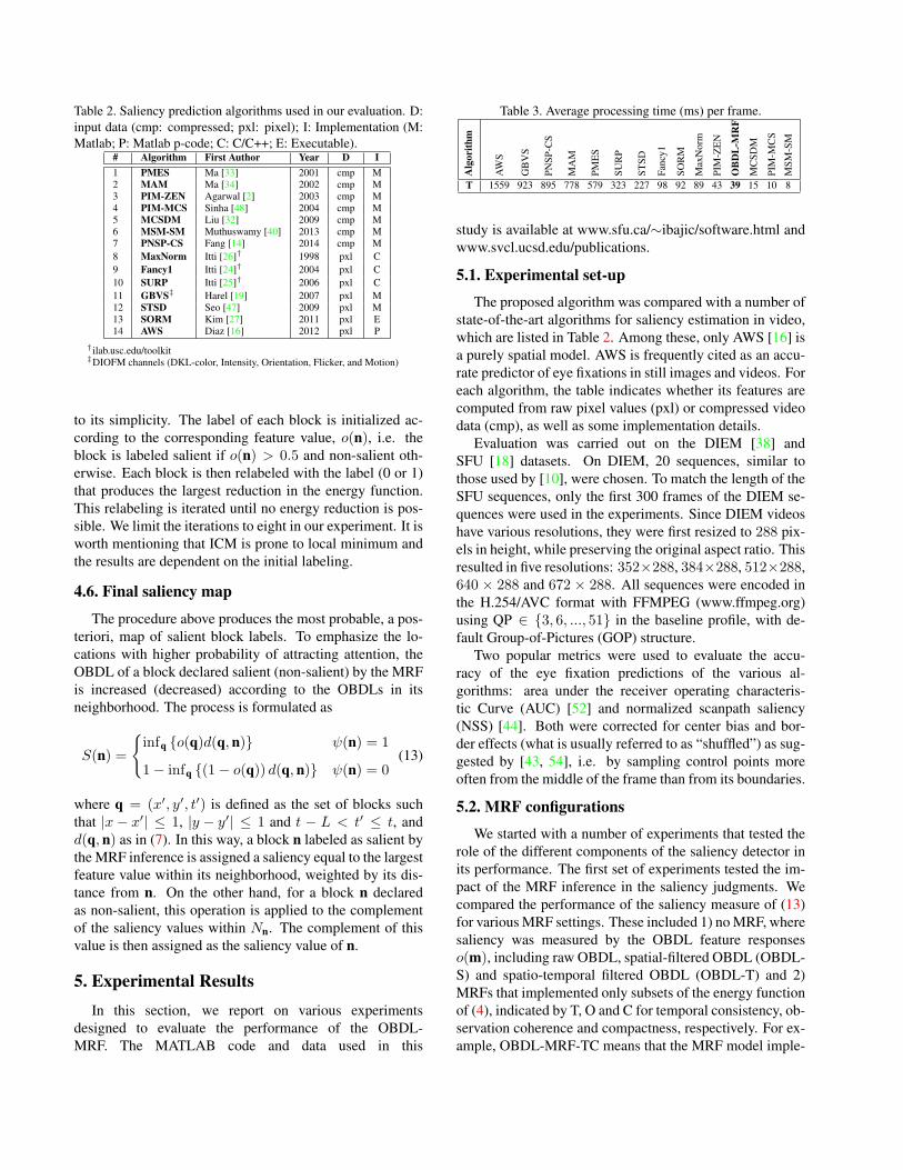
Table 2. Saliency prediction algorithms used in our evaluation. D:input data (cmp: compressed; pxl: pixel); I: Implementation (M:Matlab; P: Matlab p-code; C: C/C++; E: Executable).

# Algorithm First Author Year D I1 PMES Ma [33] 2001 cmp M2 MAM Ma [34] 2002 cmp M3 PIM-ZEN Agarwal [2] 2003 cmp M4 PIM-MCS Sinha [48] 2004 cmp M5 MCSDM Liu [32] 2009 cmp M6 MSM-SM Muthuswamy [40] 2013 cmp M7 PNSP-CS Fang [14] 2014 cmp M8 MaxNorm Itti [26]† 1998 pxl C9 Fancy1 Itti [24]† 2004 pxl C10 SURP Itti [25]† 2006 pxl C11 GBVS‡ Harel [19] 2007 pxl M12 STSD Seo [47] 2009 pxl M13 SORM Kim [27] 2011 pxl E14 AWS Diaz [16] 2012 pxl P

†ilab.usc.edu/toolkit‡DIOFM channels (DKL-color, Intensity, Orientation, Flicker, and Motion)

to its simplicity. The label of each block is initialized ac-cording to the corresponding feature value, o(n), i.e. theblock is labeled salient if o(n) > 0.5 and non-salient oth-erwise. Each block is then relabeled with the label (0 or 1)that produces the largest reduction in the energy function.This relabeling is iterated until no energy reduction is pos-sible. We limit the iterations to eight in our experiment. It isworth mentioning that ICM is prone to local minimum andthe results are dependent on the initial labeling.

4.6. Final saliency map

The procedure above produces the most probable, a pos-teriori, map of salient block labels. To emphasize the lo-cations with higher probability of attracting attention, theOBDL of a block declared salient (non-salient) by the MRFis increased (decreased) according to the OBDLs in itsneighborhood. The process is formulated as

S(n) =

infq o(q)d(q, n) ψ(n) = 1

1− infq (1− o(q)) d(q, n) ψ(n) = 0(13)

where q = (x′, y′, t′) is defined as the set of blocks suchthat |x− x′| ≤ 1, |y − y′| ≤ 1 and t − L < t′ ≤ t, andd(q, n) as in (7). In this way, a block n labeled as salient bythe MRF inference is assigned a saliency equal to the largestfeature value within its neighborhood, weighted by its dis-tance from n. On the other hand, for a block n declaredas non-salient, this operation is applied to the complementof the saliency values within Nn. The complement of thisvalue is then assigned as the saliency value of n.

5. Experimental ResultsIn this section, we report on various experiments

designed to evaluate the performance of the OBDL-MRF. The MATLAB code and data used in this

Table 3. Average processing time (ms) per frame.

Alg

orith

m

AW

S

GB

VS

PNSP

-CS

MA

M

PME

S

SUR

P

STSD

Fanc

y1

SOR

M

Max

Nor

m

PIM

-ZE

N

OB

DL

-MR

F

MC

SDM

PIM

-MC

S

MSM

-SM

T 1559 923 895 778 579 323 227 98 92 89 43 39 15 10 8

study is available at www.sfu.ca/∼ibajic/software.html andwww.svcl.ucsd.edu/publications.

5.1. Experimental set­up

The proposed algorithm was compared with a number ofstate-of-the-art algorithms for saliency estimation in video,which are listed in Table 2. Among these, only AWS [16] isa purely spatial model. AWS is frequently cited as an accu-rate predictor of eye fixations in still images and videos. Foreach algorithm, the table indicates whether its features arecomputed from raw pixel values (pxl) or compressed videodata (cmp), as well as some implementation details.

Evaluation was carried out on the DIEM [38] andSFU [18] datasets. On DIEM, 20 sequences, similar tothose used by [10], were chosen. To match the length of theSFU sequences, only the first 300 frames of the DIEM se-quences were used in the experiments. Since DIEM videoshave various resolutions, they were first resized to 288 pix-els in height, while preserving the original aspect ratio. Thisresulted in five resolutions: 352×288, 384×288, 512×288,640 × 288 and 672 × 288. All sequences were encoded inthe H.254/AVC format with FFMPEG (www.ffmpeg.org)using QP ∈ 3, 6, ..., 51 in the baseline profile, with de-fault Group-of-Pictures (GOP) structure.

Two popular metrics were used to evaluate the accu-racy of the eye fixation predictions of the various al-gorithms: area under the receiver operating characteris-tic Curve (AUC) [52] and normalized scanpath saliency(NSS) [44]. Both were corrected for center bias and bor-der effects (what is usually referred to as “shuffled”) as sug-gested by [43, 54], i.e. by sampling control points moreoften from the middle of the frame than from its boundaries.

5.2. MRF configurations

We started with a number of experiments that tested therole of the different components of the saliency detector inits performance. The first set of experiments tested the im-pact of the MRF inference in the saliency judgments. Wecompared the performance of the saliency measure of (13)for various MRF settings. These included 1) no MRF, wheresaliency was measured by the OBDL feature responseso(m), including raw OBDL, spatial-filtered OBDL (OBDL-S) and spatio-temporal filtered OBDL (OBDL-T) and 2)MRFs that implemented only subsets of the energy functionof (4), indicated by T, O and C for temporal consistency, ob-servation coherence and compactness, respectively. For ex-ample, OBDL-MRF-TC means that the MRF model imple-

os ailss ab

laic

Stefanbw

s

Mobile

mtninHall

Mother

blicbntbrpas

SoccerBus

Gardenabbhp6t

Harbour ai ds

swffnim

Foreman

Tempetem

gufcipnbtucf

CrewCity

OBDL−MRF

OBDL−MRF−TO

OBDL−MRF−OC

OBDL−MRF−O

OBDL−MRF−TC

OBDL−MRF−C

OBDL−T

OBDL−MRF−T

OBDL−S

OBDL

0.5 0.9

0.6 0.65 0.7Avg AUC’

0.6

0.8A

vg

AU

C’

Figure 2. Accuracy of various MRF settings. Each 2D color mapshows the average AUC score of each setting on each sequence.Topbar: Average AUC score for each sequence, across all settings.Sidebar: Average AUC scores each setting across all sequences.Error bars represent standard error of the mean, σ/

√n, where σ is

the sample standard deviation of n samples. Sequences from theSFU dataset are indicated with capital first letter.

mented only temporal consistency and compactness. Thiswas implemented by setting subsets of the temperature val-ues to infinity. In our example, To = ∞. The temperatureconstants were otherwise set to 1. The temporal support pa-rameter L of Section 4.2 was set to 500ms. Fig. 2 showsthe average AUC score of the various MRF settings, acrosstest sequences. The average AUC performance across se-quences/settings is shown in the sidebar/topbar. Note thatthe simple temporally filtered OBDL (OBDL-T) achievesgood performance. The global fusion of saliency informa-tion, by the MRF provides some additional gains. In gen-eral, the addition of more components to the energy func-tion results in improved predictions, with best results pro-duced by the full-blown OBDL-MRF.

5.3. Comparison to the state­of­the­art

A set of experiments was performed to compare theOBDL-MRF to state-of-the-art saliency algorithms. Theseexperiments used quantization parameter QP = 30, i.e. rea-sonably good video quality - average peak signal-to-noise(PSNR) across encoded sequences of 35.8 dB.

We start by comparing the processing times of the vari-ous saliency measures in Table 3. All times report to im-plementation on an Intel (R) Core (TM) i7 CPU at 3.40GHz and 16 GB RAM running 64-bit Windows 8.1. Asexpected, compressed-domain measures tend to require farless processing time than their pixel-domain counterparts.The proposed OBDL-MRF, implemented in MATLAB, re-quired an average of 39 ms per video frame. While this isslower than some of the compressed-domain algorithms, itenables the computation of saliency at close to 30 fps. Thisis enough for most applications of computer vision.

Fig. 3 shows the average AUC (top figure) and NSSscores (bottom figure) of various algorithms, across test se-

ailablaic ss

blicbHall

Stefan os

Mobilebwsabb

Mother

Soccerswff ds pa

s

mtnin

Gardenmg

Harbour ai

Busnimntbr

Foreman tu

cfhp6tpnb

Crew

TempeteufciCity

OBDL−MRF

MaxNorm

Fancy1

SURP

STSD

GBVS

AWS

PIM−ZEN

SORM

PIM−MCS

PMES

PNSP−CS

MAM

MCSDM

MSM−SM

0.3 0.9

0.5 0.6 0.7Avg AUC’

0.4

0.6

0.8

Avg A

UC

’

abl

mtnin

Mobile ai

lss ai

cabbblicbswffHall

Stefanbw

s os

Mother

Soccerpas

Gardenpnbntbr uf

ci ds

Harbour ai

hp6tnim m

gBustucf

Foreman

Crew

TempeteCity

OBDL−MRF

Fancy1

MaxNorm

PIM−ZEN

PMES

STSD

PIM−MCS

MSM−SM

SORM

GBVS

SURP

AWS

MAM

PNSP−CS

MCSDM

−0.4 5.4

0.5 1Avg NSS’

0

1

2

3

Avg N

SS

’

Figure 3. Accuracy of various saliency algorithms over the twodatasets according to (top) AUC and (bottom) NSS scores.

quences. On average, pixel-based methods perform betterthan those based on compressed video. This trend is how-ever disrupted by the OBDL-MRF, which achieves the bestperformance. Figure 5 illustrates the differences betweenthe saliency predictions of various algorithms.

The performances of the different saliency measureswere also evaluated with a multiple comparison test [21].This involves computing, for each sequence and measure,both the average score (across all frames) of the saliencymeasure and the 95% confidence interval for the averagescore. A set of top performers is then selected for the se-quence. This includes the measure of highest average scoreand all other measures whose 95% confidence interval over-laps with that of the highest-scoring measure. The numberof appearances of the different saliency measures among thetop performer class is shown in Fig. 4(a). Again, pixel-based methods tend to do better than compressed-basedmethods and all methods underperform the OBDL-MRF.

5.4. Sensitivity to the amount of compression

Since a compressed video representation always involvessome amount of information loss, it is important to deter-

0 5 10 15 20

OBDL−MRF

PMES

MAM

PIM−ZEN

PIM−MCS

MCSDM

MSM−SM

PNSP−CS

MaxNorm

Fancy1

SURP

GBVS

STSD

SORM

AWS

AUC

0 5 10 15 20

NSS

24 27 30 33 36 39 42 45 480.52

0.54

0.56

0.58

0.6

0.62

0.64

0.66

0.68

0.7

Average PSNR (dB)

Avera

ge A

UC

OBDL−MRF

PMES

MAM

PIM−ZEN

PIM−MCS

MCSDM

MSM−SM

PNSP−CS

MaxNorm

Fancy1

SURP

GBVS

STSD

AWS

24 27 30 33 36 39 42 45 480.1

0.2

0.3

0.4

0.5

0.6

0.7

0.8

0.9

1

Average PSNR (dB)

Av

era

ge

NS

S

OBDL−MRF

PMES

MAM

PIM−ZEN

PIM−MCS

MCSDM

MSM−SM

PNSP−CS

MaxNorm

Fancy1

SURP

GBVS

STSD

AWS

a) b)Figure 4. a) Number of appearances among top performers, under AUC and NSS. b) Impact of average PSNR on saliency predictions.

Human Map OBDL-MRF PMES MAM PIM-ZEN PIM-MCS MCSDM MSM-SM

PNSP-CS MaxNorm Fancy1 SURP GBVS STSD SORM AWS

Figure 5. Saliency maps obtained by various algorithms on a video frame.

mine the sensitivity of the saliency measure to the amountof this loss. This question is particularly pertinent for theOBDL, since the predictive power of bit counting couldchange dramatically across compression regimes. Obvi-ously, in the limit of “zero-bit encoding,” the proposedOBDL-MRF will not be a very good saliency predictor. Tostudy this question, we repeated the experiments above fordifferent amounts of compression loss, by varying the QPparameter. The quality of the encoded video, measured interms of PSNR, drops as the QP increases. Fig. 4(b) showshow the average AUC and NSS scores change as a func-tion of the average PSNR (across sequences), by choosingQP ∈ 3, 6, ..., 51. Interestingly, some of the methods thatexhibit largest sensitivity to compression artifacts (such asAWS or GBVS) are not compressed-domain approaches.

Somewhat surprisingly, saliency predictions degrade forboth very low and high quality video. For most methods,it appears that an intermediate PSNR leads to the best per-formance. This could be because, at intermediate PSNRs,compression algorithms act as mild low-pass filtering op-erators, eliminating some of the video sequence noise. Itappears that many of the algorithms are sensitive to suchnoise. With respect to the OBDL-MRF, the accuracy ofsaliency predictions degrades substantially at the extremesof the compression range. While at low rates there are toofew bits to enable a precise measurement of saliency, at highrates there are too many bits available, and all image regionsbecome salient. In any case, the OBDL-MRF achieves thetop scores for the overwhelming majority of the compres-

sion range. It is also encouraging that saliency estimation ismost accurate in the middle of this range, since this is thepreferred operating point for most vision applications.

6. Conclusion

We proposed a model of visual saliency based on thecompressibility principle. While, at a high level, this is sim-ilar to well-known saliency models, such as those based onself-information and surprise, it has the distinct advantageof being readily available at the output of any video encoder,which already exists in most modern cameras. Furthermore,the compressibility measure now proposed naturally takesinto account the trade-off between spatial and temporal in-formation, because the video encoder already performs rate-distortion optimization to produce the best predictions fordifferent video regions. In this sense, the proposed solu-tion is a much more sophisticated measure of compressibil-ity than previous measures, based on reconstruction erroror cruder measurements of self information. The resultingsaliency measure was shown highly accurate for the pre-diction of eye fixations, achieving state of the art resultson standard benchmarks. This is complemented by verylow complexity, which makes it appropriate for in-camerasaliency estimation.Acknowledgments: This work was supported inpart by NSERC grant RGPIN 327249, NSF awardIIS-1208522, and Cisco Research Award CG#573690.

References[1] E. H. Adelson and J. R. Bergen. Spatiotemporal energy mod-

els for the perception of motion. J. Opt. Soc. Am, 2(2):284–299, 1985. 3

[2] G. Agarwal, A. Anbu, and A. Sinha. A fast algorithm to findthe region-of-interest in the compressed MPEG domain. InProc. IEEE ICME’03, volume 2, pages 133–136, 2003. 2, 6

[3] S. M. Anstis and D. M. Mackay. The perception of ap-parent movement [and discussion]. Philosophical Transac-tions of the Royal Society of London. B, Biological Sciences,290(1038):153–168, 1980. 3

[4] F. Attneave. Informational aspects of visual perception. Psy-chological Review, 61:183–193, 1954. 1

[5] H. Barlow. Cerebral cortex as a model builder. In Models ofthe Visual Cortex, pages 37–46, 1985. 1

[6] H. Barlow. Redundancy reduction revisited. Network: Com-putation in Neural Systems, 12:241–253, 2001. 1

[7] J. Besag. Spatial interaction and the spatial analysis of latticesystems. Journal of the Royal Statistical Society. Series B,36:192–236, 1974. 4

[8] J. Besag. On the statistical analysis of dirty pictures. Journalof the Royal Statistical Society. Series B, 48:259–302, 1986.4, 5

[9] A. Borji and L. Itti. State-of-the-art in visual attention model-ing. IEEE Trans. Pattern Anal. Mach. Intell., 35(1):185–207,2013. 1, 2

[10] A. Borji, D. N. Sihite, and L. Itti. Quantitative analysisof human-model agreement in visual saliency modeling: Acomparative study. IEEE Trans. Image Process., 22(1):55–69, 2013. 2, 6

[11] N. Bruce and J. Tsotsos. Saliency based on information max-imization. Advances in Neural Information Processing Sys-tems, 18:155, 2006. 1, 3

[12] T. M. Cover and J. A. Thomas. Elements of InformationTheory. Wiley-Interscience, 2 edition, 2006. 1

[13] B. Efron and R. Tibshirani. An introduction to the bootstrap,volume 57. CRC press, 1993. 4

[14] Y. Fang, W. Lin, Z. Chen, C. M. Tsai, and C. W. Lin. Avideo saliency detection model in compressed domain. IEEETrans. Circuits Syst. Video Technol., 24(1):27–38, 2014. 2, 6

[15] D. Gao and N. Vasconcelos. On the plausibility of thediscriminant center-surround hypothesis for visual saliency.Journal of Vision, 8, 7:1–18, 2008. 1

[16] A. Garcia-Diaz, X. R. Fdez-Vidal, X. M. Pardo, and R. Dosil.Saliency from hierarchical adaptation through decorrelationand variance normalization. Image and Vision Computing,30(1):51–64, 2012. 2, 3, 6

[17] S. Geman and D. Geman. Stochastic relaxation, gibbs distri-bution and the Bayesian restoration of images. IEEE Trans.Pattern Anal. Mach. Intell., 6(6):721–741, 1984. 5

[18] H. Hadizadeh, M. J. Enriquez, and I. V. Bajic. Eye-trackingdatabase for a set of standard video sequences. IEEE Trans.Image Process., 21(2):898–903, Feb. 2012. 4, 6

[19] J. Harel, C. Koch, and P. Perona. Graph-based visualsaliency. Advances in neural information processing sys-tems, 19:545–552, 2007. 6

[20] D. Helbing and P. Molnar. Social force model for pedestriandynamics. Physical review E, 51(5):4282–4286, 1995. 1

[21] Y. Hochberg and A. C. Tamhane. Multiple comparison pro-cedures. John Wiley & Sons, Inc., 1987. 7

[22] X. Hou and L. Zhang. Saliency detection: A spectral residualapproach. In Proc. IEEE CVPR’07, pages 1–8, 2007. 2, 3

[23] X. Hou and L. Zhang. Dynamic visual attention: Searchingfor coding length increments. Advances in Neural Informa-tion Processing Systems, 21:681–688, 2008. 2, 3

[24] L. Itti. Automatic foveation for video compression using aneurobiological model of visual attention. IEEE Trans. Im-age Process., 13(10):1304–1318, 2004. 6

[25] L. Itti and P. F. Baldi. Bayesian surprise attracts human atten-tion. Advances in Neural Information Processing Systems,19:547–554, 2006. 1, 3, 6

[26] L. Itti, C. Koch, and E. Niebur. A model of saliency-basedvisual attention for rapid scene analysis. IEEE Trans. PatternAnal. Mach. Intell., 20(11):1254–1259, 1998. 1, 3, 4, 6

[27] W. Kim, C. Jung, and C. Kim. Spatiotemporal saliencydetection and its applications in static and dynamic scenes.IEEE Trans. Circuits Syst. Video Technol., 21(4):446–456,2011. 6

[28] D. Knill and W. Richards. Perception as Bayesian Inference.Cambridge Univ. Press, 1996. 1

[29] E. Kreyszig. Introductory mathematical statistics: principlesand methods. Wiley New York, 1970. 4

[30] S. Z. Li. Markov random field modeling in image analysis.Springer Science & Business Media, 2009. 4

[31] X. Li, H. Lu, L. Zhang, X. Ruan, and M. H. Yang. Saliencydetection via dense and sparse reconstruction. In Proc. IEEEICCV’13, pages 2976–2983, 2013. 2, 3

[32] Z. Liu, H. Yan, L. Shen, Y. Wang, and Z. Zhang. A motion at-tention model based rate control algorithm for H. 264/AVC.In The 8th IEEE/ACIS International Conference on Com-puter and Information Science (ICIS’09), pages 568–573,2009. 2, 6

[33] Y. F. Ma and H. J. Zhang. A new perceived motion based shotcontent representation. In Proc. IEEE ICIP’01, volume 3,pages 426–429, 2001. 2, 6

[34] Y. F. Ma and H. J. Zhang. A model of motion attention forvideo skimming. In Proc. IEEE ICIP’02, volume 1, pages129–132, 2002. 6

[35] V. Mahadevan, W. Li, V. Bhalodia, and N. Vasconcelos.Anomaly detection in crowded scenes. In Proc. IEEECVPR’10, pages 1975–1981, 2010. 2

[36] S. Mallat. A theory for multiresolution signal decomposi-tion: the wavelet representation. IEEE Trans. Pattern Anal.Mach. Intell., Vol. 11:674–693, July 1989. 1

[37] R. Margolin, A. Tal, and L. Zelnik-Manor. What makes apatch distinct? In Proc. IEEE CVPR’13, pages 1139–1146,2013. 2, 3

[38] P. K. Mital, T. J. Smith, R. L. Hill, and J. M. Henderson.Clustering of gaze during dynamic scene viewing is pre-dicted by motion. Cognitive Computation, 3(1):5–24, 2011.4, 6

[39] B. Moulden, J. Renshaw, and G. Mather. Two channels forflicker in the human visual system. Perception, 13(4):387–400, 1984. 3

[40] K. Muthuswamy and D. Rajan. Salient motion detec-tion in compressed domain. IEEE Signal Process. Lett.,20(10):996–999, Oct. 2013. 2, 6

[41] A. Oliva and A. Torralba. Building the gist of a scene: Therole of global image features in recognition. Progress inbrain research, 155:23–36, 2006. 1

[42] B. Olshausen and D. Field. Emergence of simple-cell re-ceptive field properties by learning a sparse code for naturalimages. Nature, 381:607–609, 1996. 1

[43] D. J. Parkhurst and E. Niebur. Scene content selected byactive vision. Spatial Vision, 16(2):125–154, 2003. 6

[44] R. J. Peters, A. Iyer, L. Itti, and C. Koch. Componentsof bottom-up gaze allocation in natural images. Vision Re-search, 45(18):2397–2416, 2005. 6

[45] P. Reinagel and A. M. Zador. Natural scene statistics at thecenter of gaze. Network: Computation in Neural Systems,10:1–10, 1999. 4

[46] N. Sebe and M. S. Lew. Comparing salient point detectors.Pattern Recognition Letters, 24(1):89–96, 2003. 2

[47] H. J. Seo and P. Milanfar. Static and space-time visualsaliency detection by self-resemblance. Journal of Vision,9(12):15, 2009. 1, 6

[48] A. Sinha, G. Agarwal, and A. Anbu. Region-of-interestbased compressed domain video transcoding scheme. InProc. IEEE ICASSP’04, volume 3, pages 161–164, 2004. 6

[49] A. Srivastava, A. B. Lee, E. P. Simoncelli, and S. C. Zhu. Onadvances in statistical modeling of natural images. Journalof mathematical imaging and vision, 18(1):17–33, 2003. 1

[50] C. Stauffer and W. Grimson. Adaptive background mix-ture models for real-time tracking. In Proc. IEEE CVPR’99,pages 246–252, 1999. 2

[51] G. Sullivan, J. Ohm, W.-J. Han, and T. Wiegand. Overviewof the high efficiency video coding (HEVC) standard. IEEETrans. Circuits Syst. Video Technol., 22(12):1649–1668,2012. 3

[52] J. A. Swets. Signal detection theory and ROC analysis inpsychology and diagnostics: Collected papers. LawrenceErlbaum Associates, Inc., 1996. 6

[53] R. Szeliski, R. Zabih, D. Scharstein, O. Veksler, V. Kol-mogorov, A. Agarwala, M. Tappen, and C. Rother. A com-parative study of energy minimization methods for Markovrandom fields. In Proc. ECCV’06, volume 2, pages 16–29,2006. 5

[54] B. W. Tatler, R. J. Baddeley, and I. D. Gilchrist. Visual cor-relates of fixation selection: Effects of scale and time. VisionResearch, 45(5):643–659, 2005. 6

[55] C. Wang, N. Komodakis, and N. Paragios. Markov randomfield modeling, inference & learning in computer vision &image understanding: A survey. Computer Vision and ImageUnderstanding, 117(11):1610–1627, 2013. 4

[56] T. Wiegand, G. J. Sullivan, G. Bjontegaard, and A. Luthra.Overview of the H. 264/AVC video coding standard. IEEETrans. Circuits Syst. Video Technol., 13(7):560–576, 2003. 3

[57] L. Zhang, M. H. Tong, T. K. Marks, H. Shan, and G. W. Cot-trell. SUN: A bayesian framework for saliency using naturalstatistics. Journal of Vision, 8(7), 2008. 1