how should a firm manage deteriorating inventory? should a firm manage deteriorating inventory? ......
TRANSCRIPT
How Should a Firm Manage Deteriorating Inventory?
Mark E. Ferguson College of Management
Georgia Institute of Technology 800 West Peachtree Street, NW
Atlanta, GA 30332-0520 Tel: (404) 894-4330 Fax: (404) 894-6030
Email:[email protected]
Oded Koenigsberg Graduate School of Business
Columbia University New York, NY 10027
Tel: (212) 854-7276 Fax: (212) 854-7647
Email:�[email protected]�
Submitted: June 2005, October 2005, December 2005. Accepted: January, 2006 The order of authorship is alphabetical and the authors contributed equally to the manuscript.

How Should a Firm Manage Deteriorating Inventory?
Abstract
Firms selling goods whose quality level deteriorates over time often face difficult decisions when
unsold inventory remains. Since the leftover product is often perceived to be of lower quality
than the new product, carrying it over offers the firm a second selling opportunity and the ability
to price discriminate. By doing so, however, the firm subjects sales of its new product to
competition from the leftover product. We present a two period model that captures the effect of
this competition on the firm’s production and pricing decisions. We characterize the firm’s
optimal strategy and find conditions under which the firm is better o. carrying all, some, or none
of its leftover inventory. We also show that, compared to a firm that acts myopically in the first
period, a firm that takes into account the effect of first period decisions on second period profits
will price its new product higher and stock more of it in the first period. Thus, the benefit of
having a second selling opportunity dominates the detrimental effect of cannibalizing sales of the
second period new product.
Keywords: pricing, perishable inventory, quality, internal competition, product line

1 Introduction
When firms complain of competitive pressure on their product lines, they are typically re-
ferring to the actions of other firms seeking to steal away their customers. For companies
selling perishable goods however, competition may also arise internally when the firm sells
inventory of its perishable goods that was leftover from previous periods. If their customers’
perception of the quality of the leftover units is lower than that of their new units, the left-
over units are often marked down in price. By doing so, however, the firm subjects sales of
its new units to competition. For example, Bloomingdale’s Department Store estimates that
50% (around $400M) of their total sales is sold through the use of mark-down prices. An
additional 9% ($72M) is sold to salvage retailers for pennies on the dollar to avoid excessive
cannibalization of their new designs (Berman, 2003). Thus, for some products, Blooming-
dale’s sells the older garments alongside its new garments while for other products, they
choose to dispose of the older garments to avoid cannibalizion.
The management decision to sell or dispose of older inventory is not unique to fashion
retailers; firms in many different industries selling perishable goods often replenish their
inventory with new items before all of their old items (of the same type) have been sold.
How a firm should stock and price a perishable product depends on the characteristics of
the perishable product and the cunsumer’s perceived difference in quality between an old
and new item. Before investigating the optimal pricing and stocking decisions, we first
characterize perishable products into three types based on the perceived quality level of the
aged product by the consumer.
The perceived quality level of Type 1 products does not degrade continuously over time
but, instead becomes unusable after a given date. Airline seats and hotel rooms are examples
of this type of product. Firms selling Type 1 products often set multiple prices (and
corresponding quantities) depending on the time remaining before expiration and receive zero
revenue for expired, unsold product. The practice of revenue management was developed
specifically for these type of products, a review of which is provided by Talluri and van Ryzin
(2004).
1

The perceived quality level of Type 2 products deteriorates continuously over time reach-
ing a value of zero when a new version of the item becomes available. Examples include
newspapers, textbooks and forecasts. Firms offering Type 2 products usually remove all of
the old units and replace them with new ones once they become available. The discounting
of Type 2 products often falls under the realm of dynamic pricing. Bitran and Caldentey
(2002) provide a review of dynamic pricing models along with many applications.
The perceived quality of Type 3 products deteriorates over time but does not reach a
value of zero when a replenishment of new items arrive. The deterioration does ensure,
however, that the customer values an older product lower than a newer one, thus firms sell-
ing Type 3 products must price differentiate the old and new items. Examples of Type
3 product are abundant and can be divided into two main categories. The first category
includes products whose actual functionality deteriorates over time such as fresh produce. It
is common practice in large retail stores and supermarkets, who account for approximately
50% of this market, to mark down their older produce after restocking with fresher prod-
uct. The second category includes products whose functionality does not degrade, but the
customers’ perceived utility of the product deteriorates over time. Examples include fash-
ionable clothing and high-technology products with short life cycles. Almost every fashion
goods retailer provides a discount section on their shop floor or web site where they offer
last season’s unsold designs at discounted prices. In this work, we focus on the pricing and
stocking decisions of Type 3 products when inventory of different quality levels is sold to the
same set of consumers. Therefore, it is critical to understand how the quality of a product
affects the firm’s operating and pricing decisions.
Observing the pricing and stocking policies of firms selling Type 3 products shows a wide
range of practices employed. For example, consider the opposing policies of two national
bagel chains (Bruegger’s and Chesapeake) who compete in the same markets and have similar
operating procedures. Stores of each chain begin each day facing a decision of how many
bagels to bake before opening their shops and observing demand. Despite the similarities
in their operating and market conditions, the two chains use different policies for how to
handle bagels leftover at the end of the day. Chesapeake Bagels disposes of all leftover
2

bagels while Bruegger’s Bagels carries the leftover bagels over to be sold in the next day.
Since the quality of a bagel depreciates quickly over time, Bruegger’s Bagels sells the leftover
bagels at a discounted price compared to the price of its fresh bagels, then disposes of any
bagels more than two days old since they consider them too low of a quality to sell at any
price.
Why do two firms facing similar production and market conditions handle their perishable
inventory so differently? What is clear from the bagel chains and many other industry
examples is that managers differ on how to manage the pricing and quantity decisions of
perishable product. Other examples of markets that face this problem include: a grocery
store that periodically receives shipments of fresh produce and sells it with any unsold
inventory; a high technology company that has not sold all of its previous model’s stock
before the new model design is ready for the market; and a software company that still holds
inventory of the current version of its product when the new version becomes available.
To gain intuition, we study a firm selling a perishable good that lasts for two periods
and has two states. The product is considered “new” if it is sold in the same period it was
produced, or “old” if it is sold the period after it was produced. The old units suffer a
perceived quality reduction and, therefore, provide lower valuations for the customers. In
the first period, we study the impact of allowing the firm to carry leftover units to the second
period on the firm’s first period stocking and pricing decisions. In the second period, we
model the competition between the new units with the old units that did not sell in the first
period and are carried over to the second.
The key decisions the firm must make include: the price and purchase quantity of new
units in both the first and second period, the quantity of unsold units from the first period
to make available to the customer in the second period, and the price to charge for the old
units in the second period. We solve the firm’s problem and find the optimal second-period
price of the new units remains the same, regardless of the firm’s decision to sell the old units
and is independent of the quality level of the old units. Thus, competition from the old units
only affects the firm’s second-period new units quantity decision, not its new units pricing
decision. We also find that carrying the older units allows the firm to price discriminate in
3
the second period. Further, we find thresholds for the quality level of the old units where
the firm should choose to carry all, some, or none of its unsold product over to the next
period. These results stem from the fact that demand for the new units is dependent upon
the quantity, price, and quality level of the old units competing against it.
In our first-period analysis, we extend the work of Petruzzi and Dada (1999) on a firm’s
price and quantity choice under uncertainty to the case where unsold inventory can be carried
to the next period, but at a reduced quality level. Compared to a firm that never carries
leftover product to the second period, we find a firm that does carry over, prices its new units
higher and stocks more of them in the first period. Thus, the benefit of having a second
selling opportunity (along with the ability to price discriminate) dominates the detrimental
effect of cannibalizing sales of the new units in the second period. Through a numerical
study we measure the benefit of employing an optimal policy compared to commonly used
“carry all unsold units” or “never carry any unsold units” alternative policies. For both
comparisons, we find the largest benefit when uncertainty over the market potential in the
first period is high and the cost to prepare the carried over units for the market is low
compared to the cost to purchase new units. Interestingly, the largest benefit of using an
optimal policy occurs for low quality differences (between the new and old units) for the
“never carry” policy but for medium quality differences for the “carry all” policy.
1.1 Literature Review
The problem we study has many similarities to a firm’s product line decision. To see how,
consider our scenario. A firm produces a single product and sells it in a market with an
unknown demand. When demand turns out to be lower than expected, the firm ends up
with unsold units. These units can be carried as inventory into the next period but, in
the case of perishable products, the unsold units suffer a quality reduction and become a
partial substitute for new units. Thus, the firm’s decision to carry inventory or not turns
into a product line decision as the firm must now consider the effect of potential future
cannibalization on the original product line. Thus, our work extends both the operations
literature on inventory management and the marketing literature on a firm’s product line
4
decisions. We extend the inventory management literature by showing how the internal-
competition between old units (inventory) and new units may change the firm’s current and
past decisions. We extend the product line literature by demonstrating another source for
product line extensions — the combination of stochastic demand (which may result in unsold
inventory) and the deterioration of the product.
The product line decision is one of the most important decisions a firm can make. Firms
often design their product line by segmenting their market on quality attributes, reflecting
consumers’ preferences to higher quality over lower quality products (vertically differenti-
ated). An immediate problem of introducing products with different qualities is cannibal-
ization, as some products may serve as partial substitutes for others and consumers choose
the product that maximizes their utility. Previous research has analyzed the cannibalization
problem for a monopolist (see for example; Mussa and Rosen 1978 and Moorthy 1984) and
an oligopoly (for example; Katz 1984 and Desai 2001) when the firm makes a product line
decision (usually the quality-price bundles). Gilbert and Matutes (1993) assume exogenous
quality levels for two competing products and investigate the competition between two man-
ufacturers. They find if the difference between the quality levels of the two products is
sufficiently large, both firms will find it profitable to produce. We also assume an exogenous
quality level but, in contrast, find the same firm sells both high and low quality units only
when the quality difference between them is sufficiently small. Also, in contrast to the pre-
viously mentioned work that assumes a single period and a deterministic market potential
(the firm sells every unit produced), we solve a two-period model where the market potential
is stochastic in the first period and the purchase of product involves a positive lead-time so
both the quantity and pricing decisions must be made before the market potential is realized.
The use of a two-period model with a quality parameter differentiating the old and new
inventory of a firm also has some similarities to the durable goods literature. Desai, Koenigs-
berg, and Purohit (2005) use a durability parameter to represent the competition between
new units owned by the company and previously sold units, owned by consumers, that reen-
ter the market during the second period. In both our problem and theirs, competition
occurs between units of the same product differentiated only by a perceived relative quality
5
difference. Also, with the same assumption about the distribution of consumers, the inverse
demand functions are exactly the same for both problems. A major difference between the
perishable and durable goods problems however, is in the durable goods problem, what a firm
sells in the first period competes with product produced in future periods. In our model,
what a firm doesn’t sell in the first period may be carried over to compete with the firm’s
new units in future periods. There is also a difference in the decision makers, as consumers
hold the deteriorating units in the durable goods problem while the firm holds them in the
perishable goods problem. A third difference occurs in the timing of the firm’s decisions.
In Desai et al. (2005), the selling quantity in the first period is chosen after uncertainty
in the market potential is resolved. In our model, both quantity and price decisions must
be made before uncertainty is resolved and it may be optimal for the firm to scrap some
or all of its leftover inventory to avoid competition with its new units in the next period.
Thus, one objective of our paper is to examine how the quality reduction of unsold units and
the subsequent cannibalization problem created by carrying the unsold units into the next
period affects the firm’s pricing and production decisions in a newsvendor setting.
On the inventory management side, several papers study a dynamic version of the
newsvendor model where a second order opportunity exists: Donohue (2000), Fisher and
Raman (1996), Petruzzi and Dada (1999, 2002) and Cachon and Kok (2004) provide a rep-
resentative sample of this area. Petruzzi and Dada (1999) review extensions to the newsven-
dor model where the stocking quantity and selling price are set simultaneously, before the
uncertainty in the market potential is resolved. Their linear demand case is identical to
our first period model when the conditions imply that no old units be carried over to the
second period. Thus, our first period analysis extends their model to the cases when future
consequences must be factored into current decisions. This is because unsold units today
will be carried over and sold in conjunction with new units in the future, but at a reduced
quality level.
Cachon and Kok (2004) offer a simple adjustment to the newsvendor model that accounts
for the fact that the salvage value of the unsold units depends upon the quantity (but not
the quality level) available. They show the common assumption of a constant salvage
6

value based on historical estimates may lead to poor performance when the salvage value is
actually a function of the quantity left over. In contrast to our model, they do not consider
the first-period price as a decision variable and their salvage value function assumes selling
the unsold units does not affect the sales of the new units. In this context, our model can be
described as a newsvendor model with price dependent demand that explicitly accounts for
a salvage value function that impacts new unit sales through product line cannibalization.
The rest of the paper is organized as follows. In the next section we discuss our major
modeling assumptions and present our notation. In section 3, we present our model, discuss
our results, and provide a numerical study measuring the impact on profit a firm incurs if
it chooses an extreme policy of always carrying or never carrying unsold units to the next
period. In section 4 we conclude and give directions for future research. All proofs and
derivations are included in an appendix along with three extensions: I) an infinite horizon
analysis, II) the quality of the good increases over time and III) the price of the new units
is held constant over both periods.
2 Model Development
This section describes the model and lays out the assumptions about the firm, the product,
and the market. We begin with the sequence of events. In the first period, the firm chooses
the price and quantity of new units only, before learning the maximum market potential for
the product. Next, market uncertainty is resolved and consumers make their purchasing
decisions. In the second period, there is no uncertainty about the market potential and
the firm may carry over unsold units if demand in the first period was lower than expected.
Thus, in the second period, the firm makes decisions on both new and old units; how many
leftover units to prepare for the market, what to price them, and how many new units to
purchase and what to price them.
We continue by stating the key assumptions of our model and defining an exogenous
quality parameter that represents the customer’s perceived differentiation between the new
units and the old units in the second period. We then derive inverse demand functions
7

for the new and old units based on the consumers’ utility functions. Since the problem we
describe pertains to both manufacturing firms that produce and sell their own product and
retailers who only purchase product from other firms, we use the generic term “purchase”
through the rest of this paper to represent either production or purchasing decisions.
Assumption 1. Key problem dynamics are captured in a two period model
We consider a two period model where the firm faces uncertainty in the market potential
during the first period and potential competition in the second period from product that did
not sell in the first period and is carried over to the second. Our objective is twofold. First,
we study how the presence of competition from lower quality units affects the firm’s pricing
and stocking decisions for its new units sold along side it. This is captured through our
second-period analysis. Second, the first period allows us to study how the possibility of
carrying unsold inventory to the next period affects the firm’s first-period decisions when it
only purchases new units. Thus, a two-period model is sufficient and allows us to maintain
tractability. Other recent papers that model competitive price responses using a two-period
setting include Ferrer and Swaminathan (2005), Desai et al. (2005) Ray et al. (2005), and
Ferguson and Toktay (2005).
In the first period, the firm chooses the price, P1, and quantity, x1, of its new units before
knowing the complete characterization of the market. Demand for the firm’s product is a
function of the unknown market potential and is decreasing with the firm’s price. After
demand realization, the firm may be left with unsold units and faces a choice on how many
of these units to carry over to the second period. Without loss of generality, the salvage
value of any unsold unit not carried over to the second period is normalized to zero.
Assumption 2. Consumers are heterogenous in their valuations of the product and are
distributed uniformly in the interval [0,α].
We assume consumers differ in their willingness to pay for the product. To capture this,
we model consumers who are heterogeneous in their valuations of the product’s service. We
use the parameter θ ∈ [0,α] to represent the consumers valuations of the product in anyperiod, where a consumer with a higher θ values the product more than a consumer who has
a lower θ. We assume θ is uniformly distributed between 0 and α and each consumer uses
8

at most one product in each period. Consumers in our model are strategic in their selection
between different alternatives. For example, in the second period, consumers have to decide
to purchase a new unit, an old unit or not purchase at all (in the first period there are only
two alternatives; purchasing new or not purchasing). We assume consumers purchase at
most one unit in each period and they must consume this unit in the same period (thus,
the issue of “forward looking” consumers is not relevant in this model). We further assume
there can be no stockpiling, storage or arbitrage. Next we describe our assumption on the
upper bound of consumers’ valuation.
Assumption 3. In the first period, the maximum market potential, α, is uncertain, in the
second period, it is deterministic.
This assumption is reasonable for many products where the demand in latter periods
is highly correlated to demand in the current period. For example, the introduction of
many new products can be divided into two distinct periods. An initial period (learning
period) where the firm faces large uncertainty in the market potential of the new units and a
second period where most of the uncertainty is resolved but some of the features of the model
may change. Ehrenberg and Goodhardt (2001) shows for the majority of new products,
most market uncertainty is resolved after 6 weeks. Our main goal is to show the effect of
competition between the firm’s new units with its carried over units. This assumption allows
us to isolate this effect and gain analytical tractability to the firm’s first period decisions.
In the appendix, we show our main results carry over to an infinite horizon model where
uncertainty in the market potential exist in every period.
At the beginning of the second period, the firm has Y units leftover from the previous
period, where Y can be zero if demand exceeds supply in the first period or if the firm chooses
not to carry over its unsold product. The firm can purchase new units at a price of c each
and prepare (recycle) old units at a per unit cost of h. We assume c ≥ h, otherwise it isnever profitable for the firm to carry leftover inventory. The cost of preparing the old units
includes the holding/storage cost, plus any special packaging and preparation required for
making the old units available to the market. The firm’s quantity decisions in the second
period include the number of new units, x2, and the number of old units, y, to make available
9

to the market. The quantity of new units the firm can purchase is not capacity constrained,
but the firm cannot prepare more than Y of the old units, i.e., y ≤ Y. Demand in the secondperiod is deterministic, but inversely proportional to the price and quality deterioration of
the product made available. We assume the firm acts rationally and knows at the end of
the first period exactly how many of the old units it will sell in the second period (since the
market potential in the second period is deterministic), so it only incurs a preparation cost,
h, for the y units it sells.
Assumption 4. The quality of the old units is exogenous.
To model the leftover product’s quality level, we use the parameter q, 0 ≤ q ≤ 1, to
represent how much a unit unsold in the first period deteriorates before the second period.
All unsold units from the first period deteriorate by (1 − q) before the second period andprovide the customer with a utility less than that provided by a new unit (in the appendix we
investigate the case where the consumers’ valuation for the old units remains the same but
they perceive the new units as providing higher quality). In our utility model, this implies
that a consumer’s valuation of the services from an unsold unit is qθ. Note that if q = 0,
consumers get no utility out of the unit (it has deteriorated fully) and the manufacturer does
not sell it. If q = 1, consumers view the new and old units as identical and derive equal
utility from either type. The quality level is considered exogenous, thus the firm has no
control over the deterioration of its product. Although there are many practical examples
where this is true, there may be cases where the firm can influence the quality level of the
carried over units through its spending on storage and preparation. We leave this extension
for future research.
Inverse Demand Functions
We consider the following inverse demand system (a full derivation is included in the
appendix):
P o2 = q(α− x2 − y) , P n2 = α− x2 − qy , P1 = α− x1,
where P n2 represents the price of the new units in the second period, Po2 represents the price
of the old units in the second period, and P1 represents the price of the new units in the first
10

period. Note the quality level of the old units has a different effect on the price of the new
and the old units. As the old units’ quality increases, the price of the old units increases
since they provide higher value to consumers. However, the price of the new units decreases
as the old and new units become closer substitutes and there is more (internal) competition.
To account for uncertainty in the market potential, let the upper bound of the consumer’s
valuation α be made up of two parts, A+u, where A represents the deterministic piece and u
represents the unknown piece. We assume u is a random variable independently drawn from
F (·), F is twice differentiable over [0, B], has a finite mean µ, a non-decreasing hazard rate,and its inverse function exists. This representation of demand is common in the economics
and marketing literature and can be interpreted as a case where the shape of the demand
curve is deterministic, while the scaling parameter representing the market potential has a
random component.
The inverse demand functions can now be represented as
P1 = A− x1 + u (1)
for the first period (since there are no old units available to sell in the first period, there is
only one inverse demand function) and
P n2 = A− x2 − qy + u (2)
and P o2 = q(A− x2 − y + u) (3)
for the second period. The latter functions capture the competition between the firm’s
old units with its new units. We preview the model’s parameters, random variables, and
decision variables below.
11

First period Second period
Symbol Definition Symbol Definition
Parameters A Deterministic market potential R Realization of A+ u
q Quality level Y Unsold units of x1
c Cost to purchase new units
h Cost to carry old units
B Upper limit for rand var u
RandomVars u Stochastic market potential None
DecisionVars P1 Price of new units P n2 Price of new units
x1 New units purchased x2 New units purchased
xd1 Deterministic component of x1 P o2 Price of old units
z Safety stock component of x1 y Old units made available
Parameters and Variables
3 Analysis
To find the subgame perfect equilibrium, we solve the problem using backward induction
starting with the analysis of the second period.
3.1 Second Period: No Uncertainty
In the second period the firm knows the realization of the market potential before making
its quantity and pricing decisions. Let R represent the realization of A + u. At the start
of the second period, the firm holds Y units of leftover inventory from the first period and
may purchase additional new units. Let Π2(x2, y|Y ) represent the firm’s profit in the secondperiod when carrying Y units of unsold inventory over from the first period, Y ≥ 0. The
pricing decisions are direct outcomes of the quantity decisions. Since the firm’s second
period decisions are dependent upon the amount of leftover product carried over from the
first period, we characterize these conditions below.
12

First consider the case of Y = 0. With no leftover inventory from the pervious period,
the firm’s only decision is how many new units to purchase. The firm’s objective is
Maxx2 Π2(x2|Y = 0) = (P n2 − c)x2 where P n2 = R− x2. (4)
Next, consider the case of Y > 0 : the firm starts the second period with Y units of
leftover inventory not sold during the first period. In addition to the decision of how many
new units to purchase, x2, the firm also must decide how many old units to prepare, y. The
firm’s objective is
Maxx2,y Π2(x2, y|Y ) = (P n2 − c)x2 + (P o2 − h)y s.t. y ≤ Y (5)
where P n2 = R− x2 − qy and P o2 = q(R− x2 − y).
The firm’s objective is concave in x2 and y. Checking the first order conditions of (4) and
(5) yields several interesting results, summarized in the following Proposition.
Proposition 1 Three conditions outline the firm’s optimal second-period solution:
Condition 1. (Low quality) Suppose q < hc. The firm does not carry over leftover inventory
and the optimal second-period solution is given by the monopoly solution for the new product:
x∗2 =R−c2, P n∗2 = R+c
2, and Π∗2 =
³R−c2
´2.
Condition 2. (Medium quality) Suppose hc< q < R−c+h
R. The optimal solution is:
Case x∗2(Y ) y∗(Y ) P n∗2 (Y ) P o∗2 (Y ) Π2(Pn∗2 , P
o∗2 |Y )
Y ≤ cq−h2q(1−q)
R−2qY−c2
Y R+c2
q(R+2qY+c−2Y )2
(R−c)24+qY (qY − Y + c)− Y h
Y > cq−h2q(1−q)
(1−q)R−c+h2(1−q)
cq−h2q(1−q)
R+c2
qR+h2
(R2−2Rc)(q2−q)−qc2+2cqh−h24(q2−q)
Condition 3. (High quality) Suppose R−c+hR
≤ q. The optimal solution is:
13
Case x∗2(Y ) y∗(Y ) Pn∗2 (Y ) P o∗2 (Y ) Π2(Pn∗2 , P
o∗2 |Y )
Y < R−c2q
R−2qY−c2
Y R+c2
q(R+2qY+c−2Y )2
(R−c)24+qY (qY − Y + c)− Y h
R−c2q≤ Y ≤ qR−h
2q0 Y NA qR− qY qY R− qY 2−hY
qR−h2q≤ Y 0 qR−h
2qNA qR+h
2(qR−h)2
4q
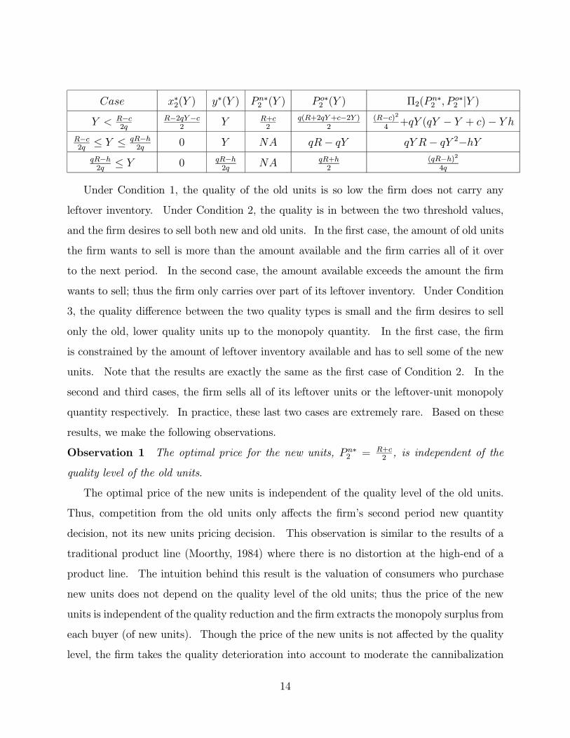
Under Condition 1, the quality of the old units is so low the firm does not carry any
leftover inventory. Under Condition 2, the quality is in between the two threshold values,
and the firm desires to sell both new and old units. In the first case, the amount of old units
the firm wants to sell is more than the amount available and the firm carries all of it over
to the next period. In the second case, the amount available exceeds the amount the firm
wants to sell; thus the firm only carries over part of its leftover inventory. Under Condition
3, the quality difference between the two quality types is small and the firm desires to sell
only the old, lower quality units up to the monopoly quantity. In the first case, the firm
is constrained by the amount of leftover inventory available and has to sell some of the new
units. Note that the results are exactly the same as the first case of Condition 2. In the
second and third cases, the firm sells all of its leftover units or the leftover-unit monopoly
quantity respectively. In practice, these last two cases are extremely rare. Based on these
results, we make the following observations.
Observation 1 The optimal price for the new units, P n∗2 = R+c2, is independent of the
quality level of the old units.
The optimal price of the new units is independent of the quality level of the old units.
Thus, competition from the old units only affects the firm’s second period new quantity
decision, not its new units pricing decision. This observation is similar to the results of a
traditional product line (Moorthy, 1984) where there is no distortion at the high-end of a
product line. The intuition behind this result is the valuation of consumers who purchase
new units does not depend on the quality level of the old units; thus the price of the new
units is independent of the quality reduction and the firm extracts the monopoly surplus from
each buyer (of new units). Though the price of the new units is not affected by the quality
level, the firm takes the quality deterioration into account to moderate the cannibalization
14

effect through its quantity decisions. As the quality level of the old units decreases, the firm
increases the number of new units it purchases and places an upper bound on the number of
old units carried over from the previous period. The next two observations give the quality
threshold levels that determine whether to sell all, some, or none of the old units.
Observation 2 There exists a threshold level for the quality of the old units, hc, below which
the firm only sells the new units.
A lower quality threshold exists such that the firm’s ratio of old unit carrying cost to its
new unit purchasing cost must fall below it before carrying over any unsold product becomes
attractive. If the customer’s perception of the quality level of the old units is so low they
are unwilling to cover the marginal carrying cost, then it is optimal for the firm not to carry.
Remember h is the total per-unit cost to carry and prepare the old units for the second
period. It not only includes the normal inventory holding cost but also any additional costs
such as packaging, special storage, labor, etc. As an example, the selling of older produce
and day-old bagels often involves a repackaging cost in addition to the regular holding cost.
Another example is electronic circuit boards, which tend to oxidize over time and must be
kept in expensive low-oxygen storage facilities if they are not used within the first few weeks
of delivery. Using the lower quality threshold, firms can make informed decisions on whether
or not the benefit of carrying their unsold inventory into future periods exceeds these cost.
Once a decision to carry the old units has been made, the criteria for whether to carry all
of the unsold product or only a portion of it is given in the next observation.
Observation 3 There exists a threshold level for the quality of the old units, R−c+hR
, above
which the firm only sells the old units, up to a quantity of min³qR−h2q, Y´.
An upper quality threshold exists, above which the firm sells all of its leftover units up to
the minimum of the number of old units available, Y, or a monopoly quantity modified by the
quality level and based on the cost structure of the old units, qR−h2q. An unsold unit with a
quality level above this upper threshold (R−c+hR
) presents a larger benefit to the firm than the
sale of a new unit, because the new unit requires the full purchase cost. Therefore, the firm
has a higher incentive to carry and prepare the old units than to purchase new ones. The
amount of old units sold however, depends on the previous period as the firm’s old unit sales
15

are constrained by the availability of the carried over units. Thus, the firm faces a capacity
constraint on the old, lower quality units but does not face a similar constraint regarding the
new, higher quality units. Since the price of the new units is not affected by the number of
old units available, this capacity constraint increases the price of the old units and increases
the cannibalization effect. In some ways, the analysis of the second period is equivalent to a
single-period product line problem with exogenous qualities. At the beginning of the second
period, the firm has to decide whether to introduce a short product line which consists of a
single product (either new higher-quality or old lower-quality) or to extend the product line
and introduce two products.
Knowing the optimal responses for the firm in the second period, we now move back
in time to the first period where the firm must make decisions without knowing the exact
market potential for its product.
3.2 First Period: With Uncertainty
In the first period, the firm only makes price and quantity decisions for its new units. The
firm faces a market potential with a stochastic component and has to take into account the
effect of its decisions on its future performance. The total market potential for the product is
A+u, where A is deterministic and known by the firm while u is stochastic and the firm only
knows its distribution. We assume A > c and u ≥ 0 to ensure the firm always purchases a
positive quantity. Since the market potential is made up of a deterministic and a stochastic
component, we divide the firm’s quantity decision x1 into two components: x1 = xd1+z, where
xd1 = A−P1 corresponds to the known market potential and z corresponds to the stochasticmarket potential. The optimal deterministic component of the quantity decision is xd1 =
A−c2
(the monopoly result of maximizing (P1 − c)x1 where P1 = A − x1) and z represents thefirm’s safety stock that the firm holds to account for the market uncertainty. Let Y be the
positive difference between the actual demand and the safety stock, Y = (z−u)+. Since thefirm knows the quality level of its leftover product before making its first period decisions, we
study the firm’s decisions when the quality is below (Case L) and above (Case H) the lower
threshold level. We only present our results for Cases L and H pertaining to Conditions 1
16

and 2 of Proposition 1 but similar results can be obtained for Condition 3 of Proposition 1.
In our experience, Cases L and H cover the vast majority of scenarios found in practice so
we restrict our presentation to these cases.
Case L:³q ≤ h
c
´In this case (L for low quality), corresponding to Condition 1 of Proposition 1, the quality
level of the leftover product is below the lower threshold so the firm never carries over unsold
inventory. In the first period, both the quantity, x1, and price, P1, must be set before
observing the size of the market. The firm’s objective in the first period is to maximize
its expected profit over the first and second periods. Let Π12 represent the firm’s expected
profit over the first and second periods which includes its revenue minus the purchase cost
plus a discount factor, ρ, applied to the second period profit.
The profit for the first period after the total market potential is realized (u = U) is the
difference between the firm’s sales revenue and cost plus its discounted second period profit:
Π12 (z, P1 | u = U) = P1
³xd1 + U
´− c
³xd1 + z
´+ ρΠ∗2 (0) , if U ≤ z
(P1 − c)³xd1 + z
´+ ρΠ∗2 (0) , if z < U
.
The firm’s first period objective is: MaxP1,z Π12 (z, P1) . Following our assumption that the
uncertain component of the market potential is continuously distributed, the firm’s expected
profit over the first and second period can be expressed as
Π12 (z, P1) =
zZ0
P1³xd1 + u
´f (u) du+
BZz
P1³xd1 + z
´f (u) du− c(xd1 + z) + ρΠ∗2 (0) . (6)
The firm’s first period decisions do not affect its second period’s profit so the firm’s objective
reduces to a single period problem. Whitin (1955) was the first to introduce a single period
problem with quantity and pricing decisions. Zabel (1970) introduced the solution method
of first optimizing P1 for a given z and then searching over the optimal trajectory to maximize
(6). Petruzzi and Dada (1999) provide an excellent review of the literature in this area and
show that (6) is concave and unimodal in z and P ∗1 (z) as long as the distribution for u has
a non-decreasing hazard rate (their other condition for a unique solution is automatically
17

satisfied by our restrictions on the parameter values). From Petruzzi and Dada (1999), the
optimal safety stock quantity is
z∗ = F−1u
ÃP ∗1 − cP ∗1
!(7)
and the optimal price is
P ∗1 =A+ c+ µ
2− Θ (z∗)
2(8)
where Θ (z∗) =RBz∗(u − z∗)f(u)du. The total purchase quantity is the combination of the
optimal deterministic and stochastic components: x∗1 = xd∗1 + z
∗.
Case H:³hc< q < A+µ−c+h
A+µ
´In this case (H for high quality), corresponding to Condition 2 in Proposition 1, the
quality level of the leftover units is sufficient for the firm to carry over the unsold inventory.
For quality levels in this range, we see from Proposition 1 the firm never carries more
than cq−h2q(1−q) units, which is the maximum amount it will sell in the second period and this
maximum amount is less than the upper limit for u. For ease of notation, let Ψ = cq−h2q(1−q)
represent this upper bound on the amount of unsold product the firm carries over to the
second period. The profit for the first period after the total market potential is realized,
(u = U) , is the difference between the firm’s revenue and cost plus its discounted future
profits:
Π12 (z, P1 | u = U) =
P1³xd1 + U
´− c
³xd1 + z
´+ ρΠ2 (Ψ) , if U ≤ z −Ψ
P1³xd1 + U
´− c
³xd1 + z
´+ ρΠ2(z − U), if z −Ψ < U ≤ z
(P1 − c)³xd1 + z
´+ ρΠ2(0), if z < U
,
where Proposition 1 gives the expressions for Π2 (Ψ) , Π2 (z − U) , and Π2 (0). Before the
uncertainty of the market potential is resolved, the firm’s expected profit is
Π12 (z, P1) =
z−ΨZ0
[P1 (A− P1 + u) + ρΠ2 (Ψ)] f (u) du (9)
18
+
zZz−Ψ
[P1 (A− P1 + u) + ρΠ2(z − u)] f (u) du
+
BZz
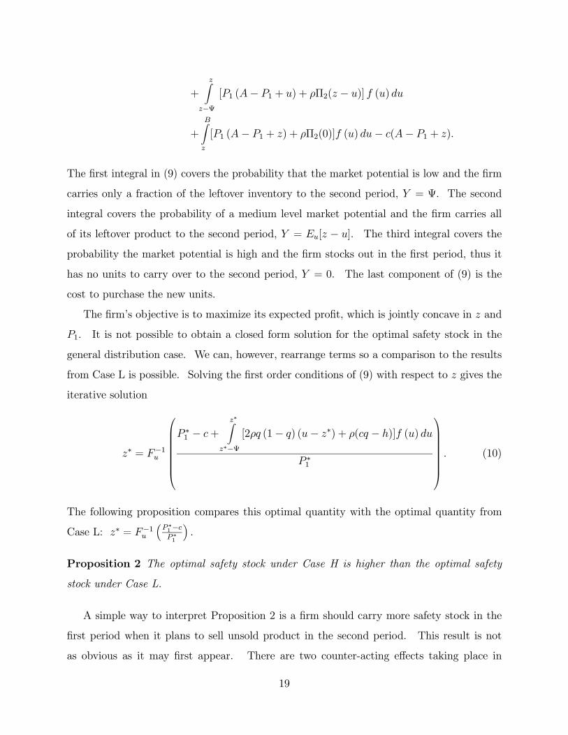
[P1 (A− P1 + z) + ρΠ2(0)]f (u) du− c(A− P1 + z).
The first integral in (9) covers the probability that the market potential is low and the firm
carries only a fraction of the leftover inventory to the second period, Y = Ψ. The second
integral covers the probability of a medium level market potential and the firm carries all
of its leftover product to the second period, Y = Eu[z − u]. The third integral covers the
probability the market potential is high and the firm stocks out in the first period, thus it
has no units to carry over to the second period, Y = 0. The last component of (9) is the
cost to purchase the new units.
The firm’s objective is to maximize its expected profit, which is jointly concave in z and
P1. It is not possible to obtain a closed form solution for the optimal safety stock in the
general distribution case. We can, however, rearrange terms so a comparison to the results
from Case L is possible. Solving the first order conditions of (9) with respect to z gives the
iterative solution
z∗ = F−1u
P ∗1 − c+
z∗Zz∗−Ψ
[2ρq (1− q) (u− z∗) + ρ(cq − h)]f (u) du
P ∗1
. (10)
The following proposition compares this optimal quantity with the optimal quantity from
Case L: z∗ = F−1u³P ∗1−cP∗1
´.
Proposition 2 The optimal safety stock under Case H is higher than the optimal safety
stock under Case L.
A simple way to interpret Proposition 2 is a firm should carry more safety stock in the
first period when it plans to sell unsold product in the second period. This result is not
as obvious as it may first appear. There are two counter-acting effects taking place in
19

the firm’s first period quantity decision. On one hand, the availability of a second selling
opportunity lowers the firm’s overage cost and induces it to produce more. Further, holding
the deteriorating units in inventory allows the firm to price discriminate between consumers,
where consumers with higher valuation for the product purchase new units and consumers
with lower valuation may purchase old units. On the other hand, the cannibalization of its
new unit sales in the second period by its old units drives its overage cost up, inducing it
to produce less in the first period. Proposition 2 shows that under Case H, the “purchase
more” effect dominates the “purchase less” effect, resulting in a larger quantity than when
the firm does not carry over its unsold inventory. We now continue the analysis by solving
for the optimal price.
Solving the first order condition of (9) with respect to P1 yields;
P ∗1 =A+ c+ µ
2− Θ (z∗)
2, (11)
which has the same relationship to z∗ as under Case L. We can now state the third propo-
sition that compares the firm’s first period price under cases L and H.
Proposition 3 The optimal first period price under Case H is higher than the optimal first
period price under Case L.
This result follows directly from the fact that (8) and (11) are equivalent but z∗ is larger
under Case H than Case L. Since Θ (z) monotonically decreases in z, then P ∗1 must be
larger under Case H. Thus, for a product whose parameter values fall under the conditions
specified by Case H, a firm stocks more product and sells it at a higher price than it does for
a product whose parameter values fall under the conditions specified by Case L. Since the
expected remaining stock from the first period under price-dependent demand increases with
both the quantity and price of the product, the leftover inventory is higher on average when
the firm decides to carry unsold product over. Propositions 2 and 3 show both the first
period quantity and price increase when the conditions are met to carry unsold inventory,
implying that the benefit of having a second selling opportunity dominates the detrimental
effect of cannibalizing sales of the new units in the second period.
20

3.3 Comparisons to a “Never-Carry” and a “Carry-All” Heuristic
In this section we provide a numerical study comparing the expected profits obtained from
using the proposed policy to those obtained from using a never-carry heuristic (NC) or a
carry-all heuristic (CA). The never-carry heuristic is where the firm never carries leftover
inventory to the second period, regardless of the conditions. The carry-all heuristic is
where the firm acts myopically (does not take into account second period profits when
first period decisions are made) in the first period but, when ending the first period with
leftover inventory, carries all the leftover units to sell in the second period. Both type
heuristics, although sub-optimal, are often found in practice as noted by our earlier bagel
chain example. We measure the percentage improvement of our proposed policy over these
clearly sub-optimal alternatives. Note the improvements are always positive as our proposed
policy represents a relaxation of both heuristics.
We begin by constructing base scenarios from the following parameter values:
u˜U [0, B], f(u) = 1B, F (u) = u
Bρ = .9
A+ µ = 100 c = 10
(A,B) = [(90, 20), (75, 50), (50, 100)] q = {hc, ..., .9, .95, .99}
hc= 0, .25, .5, .75
The cost of purchasing a new unit is normalized to c = 10, the discount rate is held constant
at ρ = .9 and the expected market potential is normalized to A+µ = 100. For our example
case where uncertainty over the market potential is uniformly distributed, any choice for
the deterministic portion of the market potential A implies a one-to-one mapping to the
upper bound of the distribution for the uncertain portion of the market potential, B. We
study three possible combinations of (A,B) pertaining to low, medium, and high degrees of
uncertainty over the original market potential for the product. The cost ratio, hc, captures
varying degrees of the cost to carry over the unsold product. A low ratio (hc= .25) may
represent a case where the only costs involved in carrying the unsold product are just the
additional handling and storage of the product while a high ratio (hc= .75) may represent
a case where the unsold product may need to be significantly updated to bring it up to the
21

current technology level of the new unit. The numerical results of our study are available
from the authors upon request.
We first measure the increase in expected profits from using our proposed optimal policy
versus the never-carry heuristic, NC. Note it is never optimal for the firm to carry unsold
inventory when q ≤ hcor h
c> 1, thus, q is varied in increments of 0.05 from h
cto 0.99.
Observing the difference in expected profits between the two policies shows that the optimal
policy yields profits as high as 15% above the profits of the NC heuristic. Through this
study, we also gain insight to the conditions where the optimal policy is most beneficial
as compared to the never-carry heuristic. In particular, firms should strongly consider
the optimal policy when: 1) Uncertainty over the market potential is high (µ is significant
compared to A), 2) The quality degradation of the unsold product is low (q is close to 1),
and 3) The cost to prepare the carried over unit for the market is low compared to the cost
to purchase new units (h << c).
We next measure the increase in expected profits from using our proposed optimal policy
versus the carry-all heuristic, CA. In this case, we provide comparisons over the entire range
of q as the carry-all heuristic carries over unsold inventory even under conditions when the
optimal policy shows it is not profitable to do so, such as when q ≤ hc. Thus, q is varied
in increments of 0.05 from .1 to 0.99. In this comparison, the optimal policy yields profits
which are as high as 11% above the profits of the CA heuristic. Similar to the comparison
with the NC heuristic, the profit penalty for using the CA heuristic also increases in the
amount of uncertainty over the market potential and with the h/c ratio. Unlike the NC
comparison however, where the larger profit penalties occur as q approaches 1 , the largest
profit penalties for using the CA heuristic occur when the quality values are in the middle
range (.4 ≤ q ≤ .7). This occurs because, for high values of q, it is often optimal for the firmto carry over all unsold product similar to the CA heuristic. For middle values of q, the firm,
under the CA heuristic, carries too much of the unsold inventory to the second period, thus
leading to increased cannibalization of the new units. When q is small, the firm under the
CA heuristic also carries “too much” unsold inventory. However, for these values of q the
cannibalization effect is less harmful since the old product is a weak substitute for the new
22

units. Note there are many other possible heuristic policies the firm may employ, such as
acting myopically in the first period but optimally in the second. The two heuristic policies
we choose, however, provide lower bounds on the firm’s expected profit for any combination
of the optimal and suboptimal policies.
4 Conclusions
We study the pricing and quantity decisions of a monopoly firm offering a perishable product
that deteriorates if the firm does not sell it immediately. We model it as a price-setting
newsvendor problem with a second selling and production opportunity. In the first period
the firm makes pricing and quantity decisions under uncertainty over the market potential
of the product. Once the market potential is realized, the firm may have product that did
not sell and must decide how many of these unsold units to carry over to the second period.
We assume the unsold units suffer from a quality reduction, such that the old units are not
a perfect substitute for new units purchased in the second period. Thus, the firm may offer
two quality types in the second period where the carried over units cannibalize sales of the
new units and the firm must trade-off between the number of carried over units to offer to
the market versus the number of new units. The trade-off appears because it costs the firm
less to carry over an unsold unit from the first period than it does to purchase a new unit,
but it must charge a lower price for the carried over units to compensate for their lower
quality.
We characterize the leftover unit’s quality as a percentage of the new unit’s quality
level and provide the firm’s optimal pricing and quantity decisions for any given quality
degradation. In our analysis of the firm’s second-period decisions, we find two quality
thresholds determine a firm’s optimal course of actions. The lower threshold determines if
a firm should carry any unsold units into the second period. A carry policy is optimal only
when the quality level exceeds a cost ratio between carrying an old unit and producing a
new unit. Thus, as the difference in quality (between the new and old units) decreases or
the difference in cost increases, a firm is more likely to carry over old units. The higher
23
quality threshold determines how much of the leftover product should be carried over. For
quality values between the lower and upper thresholds, the firm should, on the average,
carry a fraction of its unsold units to the second period. For quality values above the upper
threshold, the firm should carry all of its unsold units, up to the second period monopoly
quantity solution. All of these results extend to the infinite horizon case (presented in the
appendix).
By including price as a decision variable, we gain valuable insights into how a firm should
price its product when facing internal competition from its own carried-over units. First,
the price of the new units in the second period is not affected by competition from the old
units. Thus, the firm charges the same price for its new units regardless of whether or not
it also sells its carried over units. Second, the relationship between the price of the new
units and the amount of safety stock produced in the first period is not affected by the firm’s
decision of how many unsold units to carry over to the second period. The first period price
does change with the quality level, but only because the optimal amount of safety stock
changes. Compared to a firm that never carries leftover units to the second period, we find
a firm that does allow for units to be carried over, prices its new units higher and stocks
more of them in the first period. Thus, the benefit of having a second selling opportunity,
and to price discriminate, dominates the detrimental effect of cannibalizing sales of the new
units in the second period.
Through a numerical study, we show increases in expected profit of up to 15% are obtain-
able compared to the never-carry or carry-all heuristics that firms often employ. We perform
a sensitivity analysis to gain insight to when the improvement is the greatest. Our proposed
policy provides the most benefits compared to a never-carry heuristic when: 1) Uncertainty
over the market potential is high, 2) The cost to prepare the carried over unit for the market
is low compared to the cost to purchase new units, and 3) The quality degradation of the
unsold units is low. Compared to a carry-all heuristic, the benefits of using our proposed
policy are also largest when uncertainty and the cost ratio are high. In contrast to the
never-carry heuristic however, a firm employing a carry-all heuristic incurs the largest profit
penalties for middle values of the quality ratio between the old and the new units.
24

One contribution of our work is an extension of the product line problem. Past research
on a firm’s product line looks at the firm’s decision of whether to introduce a new product
or not as a strategic decision the firm makes ahead of time, where firms are able to decide
which product lines to introduce, how many units to produce from each product and how to
price the different products. In this research, the firm’s product line decision is contingent
on the state of demand in the previous period. More specifically, it is only when demand in
the first period is low that the firm has the option to decide which product line to introduce.
In addition, the decision is constrained by the limited quantity of inventory. Thus, the
firm does not have full control on the number of lower quality units that may be put on
the market, affecting the pricing decision as well. Our second-period analysis captures this
unique product line decision. Based on our second period results, we analyze the first-period
problem and generate insights into the effects of offering future product lines on the firm’s
current production and pricing decisions.
A second contribution of our work is an extension of the newsvendor problem with price
dependent demand. When the quality level of the carried over units is below our lower
threshold, our first period problem is exactly the same as the standard newsvendor problem
with price dependent demand and the two periods are independent. When the quality level
exceeds the lower threshold, the problem becomes more complicated as the firm’s optimal
strategy is to carry over unsold inventory when demand does not exceed supply. In this
case, the second and first period decisions depend on each other and the firm makes its first-
period decision with the consequences of these decisions on the second-period outcome in
mind. Interestingly, we find the firm increases both its first-period production quantity and
price, above the quantity and price of a firm that does not allow the possibility of carrying
unsold inventory. This is because the expected gains from selling the lower quality units
to consumers with lower valuations (if demand turns low) plus the expected gains of selling
more units in the first period at a higher price (if demand turns high) exceeds the costs of
preparing these units for a future sale and the future cannibalization loss. The firm prices
higher, even though it purchases more units, because it now has the opportunity to sell
unsold units in the future.
25
In the appendix, we offer three model extensions. In the first extension, we model the
infinite horizon case where the market potential uncertainty occurs in every period. We
show all our significant results from the second period analysis continue to hold in this more
general case. In the second extension, we allow the quality of the new units to increase
from the first to the second period. This analysis captures situations where the product
is improved between the periods, perhaps through a design change resulting in advanced
functionality. The third extension examines the impact on expected profit if a firm decides
not to change the price of the new units between the first and second period. Surprisingly,
our numeric tests indicate the penalty is small. Thus, in situations where price changes
are costly or result in a loss of consumer goodwill, a firm may manage uncertainty strictly
through changing its stocking policy without a significant impact on its profit.
We conclude with a brief note of caution. Our model is based on a linear inverse demand
function where there is uncertainty only in the maximum market potential of the product.
There may be other areas of uncertainty including total market size and price elasticity. Also,
the relationship between price and demand may be multiplicative rather than additive. It is
unclear how our results will change under these different scenarios. Finally, we restrict our
model to the case where a firm offers a single new product. Our results may not hold for
cases where the firm sells more than one product to the same set of consumers. We leave
these unanswered questions for future research.
References
[1] Berman, B., 2003, Senior Vice President and Chief Financial Of-
ficer, Bloomingdale’s. Keynote Speech at the 2003 Revenue Man-
agement and Pricing Conference, Columbia University, New York,
http://www.demingcenter.com/html files/roi/roi 3rd agenda.htm.
[2] Bitran, G., and R. Caldentey. 2002. “An Overview of Pricing Models for Revenue Man-
agement,” MIT Working Paper.
26

[3] Cachon, G., and G. Kok. 2005. “Heuristic Equilibrium in the Newsvendor Model with
Clearance Pricing,” Wharton School Working Paper, University of Pennsylvania.
[4] Desai, P., 2001. “Quality Segmentation in Spatial Markets: When Does Cannibalization
Affect Product Line Design?” Marketing Science, 20:3, 265-283.
[5] Desai, P., O. Koenigsberg, and D. Purohit. 2004. “Strategic Decentralization and Chan-
nel Coordination,” Quantitative Marketing and Economics, 2:1, 5-22.
[6] Desai, P., O. Koenigsberg, and D. Purohit. 2006. “Research Note: The Role of Produc-
tion Lead Time and Demand Uncertainty in Durable Goods Markets,” To appear in
Management Science.
[7] Donohue, K. 2000. “Efficient Supply Contracts for Fashion Goods with Forecast Up-
dating and Two Production Modes,” Management Science, 46:11, 1397-1411.
[8] Ehrenberg, A. and G. Goodhardt. 2001. “New Brands: Near-Instant Loyalty,” Journal
of Targeting, Measurement and Analysis for Marketing, 10:1, 9-16.
[9] Ferguson, M. and B. Toktay. 2005. “The Effect of Competiton on Recovery Strategies,”
To appear in Production and Operations Management.
[10] Ferrer, G. and J. Swaminathan. 2005. “Managing New and Remanufactured Products.”
To appear in Management Science.
[11] Fisher, M., and A. Raman. 1996. “Reducing the Costs of Demand Uncertainty Through
Accurate Response to Early Sales,” Operations Research, 44, 87-99.
[12] Gilbert, R., and C. Matutes. 1993. “Product Line Rivalry with Brand Differentiation,”
Indust Econom. XLI (3), 223-239.
[13] Katz, M., 1984. ”Firm-spesific differentiation and competition among multiproduct
firms,” Journal of Business. (57), 149-166.
[14] Moorthy, K. S., 1984. “Market Segmentation, Self-Selection and Product Design,”Mar-
keting Science, 3: 4, 288-305.
27
[15] Mussa, M. and S. Rosen. 1978. “Monopoly and Product Quality,” Journal of Economic
Theory, 18, 301-317.
[16] Petruzzi, N., and M. Dada. 1999. “Pricing and the Newsvendor Model: A Review with
Extensions,” Operations Research, 47, 183-194.
[17] Petruzzi, N., and M. Dada. 2002. “Dynamic Pricing and Inventory Control with Learn-
ing,” Naval Research Logistics, 49, 3, 303-325.
[18] Ray, S., T. Boyacı, and N. Aras. 2005. Optimal Prices and Trade-in Rebates for Durable
Products. To appear in Manufacturing & Service Operations Management.
[19] Talluri, K., and G. van Ryzin, 2004. The Theory and Practice of Revenue Management,
Kluwer Academic Publishers.
[20] Whitin, T. M. 1955. “Inventory Control and Price Theory,” Management Science, 2,
61—68.
[21] Zabel, E. 1970. “Monopoly and Uncertainty,” Rev. Econom.Studies 37, 205—219.
28
5 Appendix
5.1 Derivation of Inverse Demand Functions
We follow the lead of Desai Koenigsberg and Purohit (2006) and derive the demand functions from
the consumer utility functions. Note that the net utility, NU, from using a unit in the second
period is
NU = qmθ − Pm2 , (12)
where m is an indicator variable such that m = 0 if the unit is new, m = 1 if the unit is old, and
Pm2 is the second period price of new (m = 0) or old (m = 1) units.
Consider the problem facing consumers in period 2. Each consumer has to choose from one of
the three following strategies: (i) buy a new unit (N); (ii) buy an old unit (O); (iii) be inactive
(X). In consumer utility, if all three strategies are observed in equilibrium, then consumers who
follow a N strategy value the product more (i.e., have a higher θ) than consumers who follow an O
strategy, who value it more than consumers who follow an X strategy.
Now consider the lowest valuation consumer who adopts an O strategy. This consumer is
located at a point θ0 = α− x2− y on the [0,α] line and is indifferent between following an O andan X strategy. From (12), this consumer’s net utility from an O strategy is q(α− x2 − y)− P o2 ,
and the utility from following an X strategy is zero. Equating these two gives a price for the old
units of
P o2 = q(α− x2 − y).
Finally, consider the lowest valuation of the consumer who adopts an N strategy. This consumer
is located at a point θ00 = α− x2 and has to be indifferent between the N and O strategies. Thenet utility from a N strategy is α− x2 − P n2 . Similarly, the net utility from buying an old unit is
q(α− x2)− P o2 . Equating these two utilities gives a price of the new units of
P n2 = α− x2 − qy.
29

In the first period, there are only new units so their price is given by
P1 = α− x1.
5.2 Proofs
Proof of Proposition 1
Maxx2,y Π2(x2, y|Y ) = (P n2 − c)x2 + (P o2 − h)y (13)
s.t. y ≤ Y, x2 ≥ 0, y ≥ 0.
Here, P n2 = R − x2 − qy and P o2 = q(R − x2 − y). The Hessian is −2 −2q−2q −2q
, whoseleading coefficient is negative and whose determinant 4q(1 − q) is positive. Thus, the Hessian isnegative definite and the profit function is concave in (x2, y). The Lagrangean is
L(x2, y,λ) = (R− x2 − qy − c)x2 + q(R− x2 − y)y − hqr − λ(y − Y ) + ξ1x2 + ξ2y.
∂L∂x2
= −2x2 +R− 2qy − c+ ξ1
∂L∂y
= −2qx2 − 2qy − h+ qR− λ+ ξ2
Since the profit function is concave, necessary conditions and sufficient conditions for optimality
are that the first order conditions (FOC) equal 0, as well as λ(y − Y ) = 0, ξ1x2 = 0, ξ2y = 0,λ ≥ 0, ξ1 ≥ 0and ξ2 ≥ 0.
Case 1. y = Y and x2 > 0. Then λ ≥ 0, ξ2 = 0 and ξ1 = 0. Solving the FOC gives
x2 =R−c2− qY and λ = 2(q2 − q)Y − h + qc. If Y < R−c
2q, then x2 > 0 holds. The second
condition λ ≥ 0 gives 2(q2 − q)Y − h + qc ≥ 0. The prices are as follows: P n2 = R+c2and
P o2 =q(R+c−2Y (1−q))
2. Π2 = (q
2 − q)Y + (cq − h)Y + (R−c)24
.
Case 2: 0 < y < Y and x2 > 0. Then λ = 0, ξ1 = 0 and ξ2 = 0. Solving the FOC
gives x2 =R2− c−h
2(1−q) and y =qc−h2q(1−q) . The prices are P
n2 =
R+c2and P o2 =
qR+h2. Π2 =
30

(R2−2Rc)(q2−q)−qc2+2cqh−h24(q2−q) . We need the conditions 0 < qc−h
2q(1−q) < Y and R2− c−h
2(1−q) > 0 to hold
for this case to be valid.
Case 3: 0 < y < Y and x2 = 0. Then λ = 0 and ξ2 = 0. Solving the FOC gives y =qR−h2q
and
ξ1 = R(−1+q)−h+c. We need qR > h for y > 0 to hold. We also need Y > qR−h2q. In addition,
we need R(−1 + q) − h + c ≥ 0, or R ≤ c−h1−q . The prices are as follows: P
n2 = R − qR−h
2and
P o2 = q³R− qR−h
2q
´. Π2 =
(qR−h)24q
.
Case 4: y = Y and x2 = 0. Then ξ2 = 0. Solving the FOC gives λ = qR − 2Y q − h andξ1 = −R + 2qY + c. Non-negativity conditions require Y ≤ qR−h
2qand Y ≥ R−c
2q. The prices are
as follows: P n2 = R− qY and P o2 = q(R− Y ). Π2 = qY R− qY − hY .Case 5: y = 0 and x2 > 0. Then ξ1 = 0and λ = 0. Solving the FOC gives x2 =
R−c2and
ξ2 = −qc + h. The prices are P n2 = R+c2and P o2 = qR+c
2. Π2 =
(R−c)24
. This case will hold
if −qc + h ≥ 0, or h ≥ qc. To interpret this condition, notice that c is the willingness-to-payof the threshold customer at which the firm can profitably sell the new units; if the type is any
lower, the firm would make a loss. If h > qc, this means the remanufacturing cost is more than
the willingness to pay of this threshold customer for the remanufactured product.
Case 6: Both quantities 0. Then λ = 0. Solving the FOC gives ξ1 = c−R and ξ2 = −qR+h.So this cannot happen unless c−R > 0, or, c > R which is not allowed by our restrictions on c.
Thus, there are a total of five possible cases, summarized in the Table below.
Case x2 y P n2 P o2 Π2(x2, y|Y, q)1) R−2qY−c
2Y R+c
2q(R+c−2Y+2qY )
2(q2−q)Y + (cq − h)Y+ (R−c)2
4
2) R2− c−h2(1−q)
qc−h2q(1−q)
R+c2
qR+h2
(R2−2Rc)(q2−q)−qc2+2cqh−h24(q2−q)
3) 0 qR−h2q
NA q³R− qR−h
2q
´(qR−h)2
4q
4) 0 Y NA qR− qY qY R− qY − hY5) R−c
20 R+c
2qR+c
2(R−c)24
31
Case Conditions
1) Y < R−c2q, Y ≤ qc−h
2q(1−q)
2) 0 < qc−h2q(1−q) < Y, R >
c−h1−q
3) Y > qR−h2q, R ≤ c−h
1−q
4) Y ≤ qR−h2q, Y ≥ R−c
2q
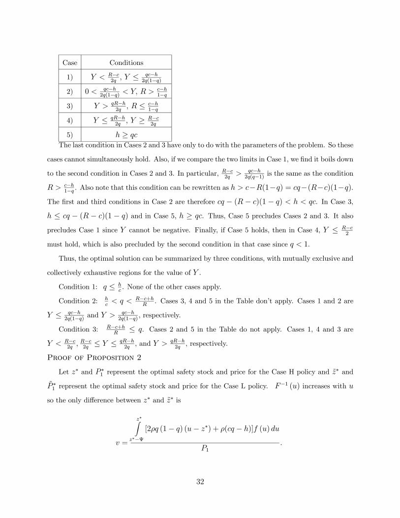
5) h ≥ qcThe last condition in Cases 2 and 3 have only to do with the parameters of the problem. So these
cases cannot simultaneously hold. Also, if we compare the two limits in Case 1, we find it boils down
to the second condition in Cases 2 and 3. In particular, R−c2q> qc−h
2q(q−1) is the same as the condition
R > c−h1−q . Also note that this condition can be rewritten as h > c−R(1−q) = cq−(R−c)(1−q).
The first and third conditions in Case 2 are therefore cq − (R − c)(1− q) < h < qc. In Case 3,h ≤ cq − (R − c)(1 − q) and in Case 5, h ≥ qc. Thus, Case 5 precludes Cases 2 and 3. It alsoprecludes Case 1 since Y cannot be negative. Finally, if Case 5 holds, then in Case 4, Y ≤ R−c
2
must hold, which is also precluded by the second condition in that case since q < 1.
Thus, the optimal solution can be summarized by three conditions, with mutually exclusive and
collectively exhaustive regions for the value of Y .
Condition 1: q ≤ hc. None of the other cases apply.
Condition 2: hc< q < R−c+h
R. Cases 3, 4 and 5 in the Table don’t apply. Cases 1 and 2 are
Y ≤ qc−h2q(1−q) and Y >
qc−h2q(1−q) , respectively.
Condition 3: R−c+hR≤ q. Cases 2 and 5 in the Table do not apply. Cases 1, 4 and 3 are
Y < R−c2q, R−c2q≤ Y ≤ qR−h
2q, and Y > qR−h
2q, respectively.
Proof of Proposition 2
Let z∗ and P ∗1 represent the optimal safety stock and price for the Case H policy and z∗ and
P ∗1 represent the optimal safety stock and price for the Case L policy. F−1 (u) increases with u
so the only difference between z∗ and z∗ is
v =
z∗Zz∗−Ψ
[2ρq (1− q) (u− z∗) + ρ(cq − h)]f (u) du
P1.
32
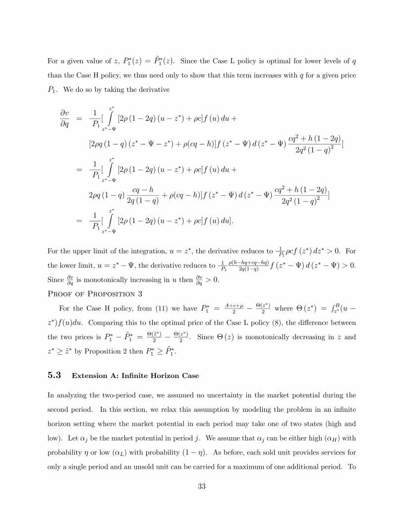
For a given value of z, P ∗1 (z) = P∗1 (z). Since the Case L policy is optimal for lower levels of q
than the Case H policy, we thus need only to show that this term increases with q for a given price
P1. We do so by taking the derivative
∂v
∂q=
1
P1[
z∗Zz∗−Ψ
[2ρ (1− 2q) (u− z∗) + ρc]f (u) du+
[2ρq (1− q) (z∗ −Ψ− z∗) + ρ(cq − h)]f (z∗ −Ψ) d (z∗ −Ψ)cq2 + h (1− 2q)2q2 (1− q)2 ]
=1
P1[
z∗Zz∗−Ψ
[2ρ (1− 2q) (u− z∗) + ρc]f (u) du+
2ρq (1− q) cq − h2q (1− q) + ρ(cq − h)]f (z∗ −Ψ) d (z∗ −Ψ)
cq2 + h (1− 2q)2q2 (1− q)2 ]
=1
P1[
z∗Zz∗−Ψ
[2ρ (1− 2q) (u− z∗) + ρc]f (u) du].
For the upper limit of the integration, u = z∗, the derivative reduces to 1P1ρcf (z∗) dz∗ > 0. For
the lower limit, u = z∗−Ψ, the derivative reduces to 1P1
ρ(h−hq+cq−hq)2q(1−q) f (z∗ −Ψ) d (z∗ −Ψ) > 0.
Since ∂v∂qis monotonically increasing in u then ∂v
∂q> 0.
Proof of Proposition 3
For the Case H policy, from (11) we have P ∗1 =A+c+µ2− Θ(z∗)
2where Θ (z∗) =
RBz∗(u −
z∗)f(u)du. Comparing this to the optimal price of the Case L policy (8), the difference between
the two prices is P ∗1 − P ∗1 = Θ(z∗)2− Θ(z∗)
2. Since Θ (z) is monotonically decreasing in z and
z∗ ≥ z∗ by Proposition 2 then P ∗1 ≥ P ∗1 .
5.3 Extension A: Infinite Horizon Case
In analyzing the two-period case, we assumed no uncertainty in the market potential during the
second period. In this section, we relax this assumption by modeling the problem in an infinite
horizon setting where the market potential in each period may take one of two states (high and
low). Let αj be the market potential in period j. We assume that αj can be either high (αH) with
probability η or low (αL) with probability (1− η). As before, each sold unit provides services for
only a single period and an unsold unit can be carried for a maximum of one additional period. To
33

distinguish our results from the two-period model, we place a hat (ˆ) above the decision variables
in this section. For each period j, the firm faces the inverse demand functions
Pn,j = αj − xj − qyj and
Po,j = q(αj − xj − yj)
where yj is the number of the unsold units the firm carries over from the previous period and xj
is the number of new units the firm chooses to sell in period j after learning the realization of the
market potential αj.
To keep the formulation tractable, we make the following assumptions: 1) the firm purchases
product before knowing the state of the market potential for that period but can reduce the quantity
to sell after learning the state, 2) all product carried over to the next period must be sold at a
market clearing price, and 3) the parameter values meet the condition that when the firm carries
inventory (when αj = αL) the amount carried is greater than or equal to the optimal amount of old
units the firm wants to sell in the next period (we assume that all other units can be scrapped at
zero per unit costs). These assumptions along with the inclusion of a discount factor ρ, 0 ≤ ρ ≤ 1,allow a steady state solution so the optimal decision variables stay constant over time. Thus, we
drop the period notation j for the remainder of this section.
At the beginning of each period the firm can be in one of two states: holding inventory (y > 0) -
state 1 or not holding inventory (y = 0) - state 0. The fact that the state space consists of only two
states is due to our assumption that if αj = αL, the firm keeps the same number of unsold units
for the next period independent of the firm’s state at the beginning of the period. This assumption
holds if the difference between αL and αH is sufficiently large (the analysis for other cases can be
obtained from the authors by request but do not change our results below). The decisions the firm
makes are state dependent and occur in the following timeline. At the beginning of each period
the firm purchases Q0 or Q1 if the firm is in state 0 or 1 respectively. After observing the market
potential, if αj = αH the firm sells all Q0 if in state 0 or Q1 new units and y old units if in state
1. If αj = αL the firm sells x0 new units if in state 0 or x1 new units and y old units if in state
34

1. The expected profits when the firm starts the period with y > 0 and y = 0 are respectively:
1) Π (y) = ηh(αH − Q1 − qy)Q1 + q(αH − Q1 − y)y − cQ1 + ρΠ (0)
i+
(1− η)h(αL − x1 − qy)x1 + q(αL − x1 − y)y − cQ1 − hy + ρΠ (y)
i,
2) Π (0) = ηh(αH − Q0)Q0 − cQQ + ρΠ (0)
i+
(1− η)h(αL − x0 − qy)x0 + q(αL − x0 − y)y − cQ0 − hy + ρΠ (y)
i.
With simple arithmetic manipulations we get Π (y) as a function of Π (0);
Π (y) =1
−1 + ρ(− y (qαL − qy − h)− η
hαH
³Q1 + qy
´− y
hqαL − h+ 2qQ1
i− Q21
i+ηρ
h−x20 (1− η) + η
³αH − Q1 − Q0
´ ³Q0 − Q1
´i+ηρ (αLx0 (1− η) + qy [y − αL + (αL + 2Q1 − αH) η])
+xQ1 (1− η) (1− ηρ) (x1 + q2y − αL) + chQ1 (1− ηρ) + ηρQ0
i).
The first order conditions with respect to Q1, Q0, x1, x0 and y yields:
Q∗0 =ηαH − c2η
, (14)
x∗0 =αL2,
Q∗1 =η[αH(1− q) (1− ηρ) + h (1− η)]− c (1− ηρ) [1− q (1− η)]
2η(1− q) (1− ηρ),
x∗1 =(1− ηρ) [αL(1− q)− cq] + h (1− η)
2(1− q) (1− ηρ), and
y∗ =cq (1− ηρ)− h (1− η)
2q(1− q) (1− ηρ).
The optimal prices of the new units are independent of the initial inventory state and are P ∗n =ηαH+c2η
if αj = αH and P∗n =
αL2if αj = αL. The optimal prices of the old units (relevant only if
y > 0) are P ∗o =12
hqαH − qc1−ηη + h(1−η)
1−ρηiif αj = αH and P
∗o =
q(αL−c)(1−ρη)+h(1−η)2(1−ρη) if αj = αL.
We now explore how our main findings from the two-period model compare to the infinite
35

horizon results. Observation 1 states that the optimal price for the new units is independent of
the quality level of the old units. This result holds for the infinite horizon model as P ∗n is not
a function of q. Observation 2 states that a lower threshold exist (q = hc) below which the firm
does not carry inventory to the next period. This result also holds for the infinite horizon model.
Note that for y∗ > 0 then q > hc> h(1−η)
c(1−ηρ) . If there is no discounting (ρ = 1), this condition is
exactly the same as in Observation 1. With discounting (ρ < 1), the condition requires a lower
quality level of the old units than does the two-period model. This result is intuitive because in
the infinite horizon model the firm can carry any unsold new units over to the next period, thus
the firm’s overage cost decreases. Observation 3 states that an upper threshold exist above which
the firm only wants to sell old units. We can not test this result for the infinite horizon case by
checking if conditions exist where x∗1 ≤ 0 since we allow the firm to set the selling quantity after
observing the market potential. Thus, x∗1 is always positive because the cost to purchase them is
a sunk cost and the firm always prefers to make available “free” new units over “free” old units.
We can however test if conditions exist for Q∗1 ≤ 0. In fact they do if q > ηαH−c+hηηαH−c+cη , thus this
result also holds for the infinite horizon case.
5.4 Extension B: Increasing Quality - New Product Has Quality Level 1 + q
In our basic model, we assumed that the consumers’ valuation of the new units remained constant
from one period to the next and that their valuation of a left-over units degrades in relation to
the new units. While this assumption is true for most grocery perishables (where, for example,
most consumers value a fresh bagel the same from one day to the next), it is not always the case
for markets where new models are introduced. If the new models contain advanced functionality
over the older models they are replacing then it is reasonable to assume that consumers will place
a higher valuation on the new model and thus, the product will have a higher reservation price
than the new units in the previous period (a notable exception is the personal computer industry
where prices for state of the art computers have remained constant from year to year despite the
dramatic advances in their capabilities). In this section we assume that the consumers’ valuation
for the old model remains the same but they perceive the new model as providing higher quality.
Assume that the consumers’ perceived value for each new unit is (1+ q) times the valuation of
36
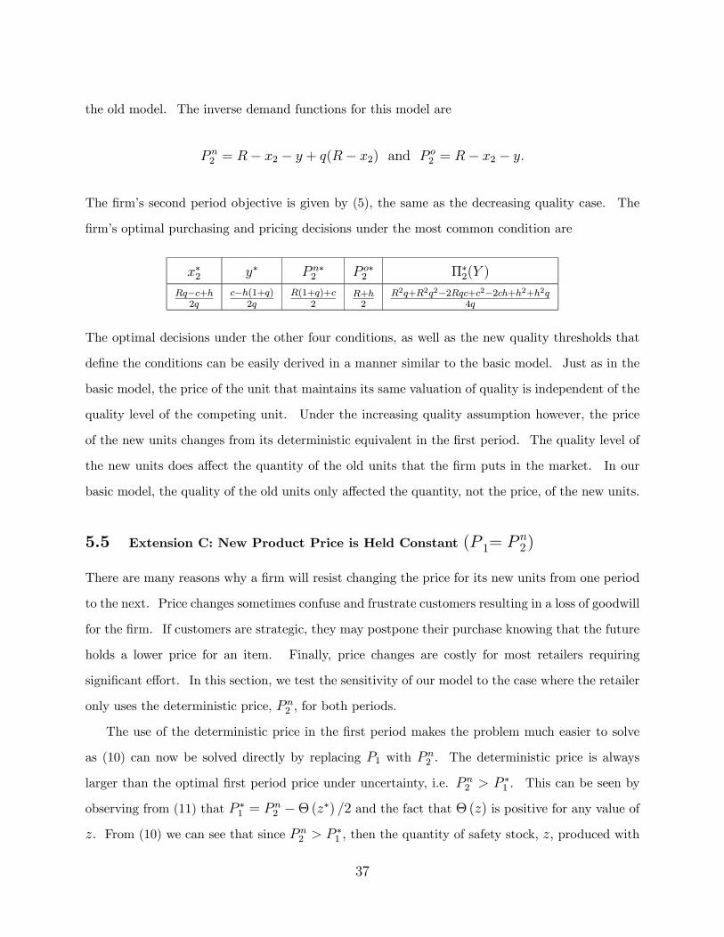
the old model. The inverse demand functions for this model are
P n2 = R− x2 − y + q(R− x2) and P o2 = R− x2 − y.
The firm’s second period objective is given by (5), the same as the decreasing quality case. The
firm’s optimal purchasing and pricing decisions under the most common condition are
x∗2 y∗ P n∗2 P o∗2 Π∗2(Y )Rq−c+h2q
c−h(1+q)2q
R(1+q)+c2
R+h2
R2q+R2q2−2Rqc+c2−2ch+h2+h2q4q
The optimal decisions under the other four conditions, as well as the new quality thresholds that
define the conditions can be easily derived in a manner similar to the basic model. Just as in the
basic model, the price of the unit that maintains its same valuation of quality is independent of the
quality level of the competing unit. Under the increasing quality assumption however, the price
of the new units changes from its deterministic equivalent in the first period. The quality level of
the new units does affect the quantity of the old units that the firm puts in the market. In our
basic model, the quality of the old units only affected the quantity, not the price, of the new units.
5.5 Extension C: New Product Price is Held Constant (P 1= Pn2)
There are many reasons why a firm will resist changing the price for its new units from one period
to the next. Price changes sometimes confuse and frustrate customers resulting in a loss of goodwill
for the firm. If customers are strategic, they may postpone their purchase knowing that the future
holds a lower price for an item. Finally, price changes are costly for most retailers requiring
significant effort. In this section, we test the sensitivity of our model to the case where the retailer
only uses the deterministic price, P n2 , for both periods.
The use of the deterministic price in the first period makes the problem much easier to solve
as (10) can now be solved directly by replacing P1 with Pn2 . The deterministic price is always
larger than the optimal first period price under uncertainty, i.e. P n2 > P∗1 . This can be seen by
observing from (11) that P ∗1 = Pn2 −Θ (z∗) /2 and the fact that Θ (z) is positive for any value of
z. From (10) we can see that since P n2 > P∗1 , then the quantity of safety stock, z, produced with
37
the deterministic price is always larger than the amount produced with the optimal price. Thus,
the firm prices higher and produces more when using the deterministic price heuristic.
To test how much of a penalty the firm incurs for using this constant price heuristic, we reran
our numerical example described in the previous section with the firm using the heuristic and
compared the expected profits with the original expected profits obtained using the optimal policy.
As expected, the penalty increases with the amount of uncertainty and is always higher under the
carry policy than the no carry policy. Surprisingly, the penalty is small: The maximum profit
penalty was 0.02 percent, occurring in the high uncertainty case (A = 50, B = 100 corresponding
to a coefficient of variation = 0.29). While gross generalizations from such a small sample should
not be made, the study does indicate that the deterministic price heuristic may be quite good and
the need for stochastic optimization of both price and quantity may have been overstated in the
previous literature.
38

The authors would like to thank Preyas Desai, Rajeev Kohli, Serguei Netessine, Devavrat
Debu Purohit, Beril Toktay and Paul Zipkin for their important comments on various
drafts of this article.