How Should Inventory Investment be Measured in

National Accounts?

By Marshall Reinsdorf and Jennifer Ribarsky* US Bureau of Economic Analysis

Washington, DC Marshall.Reinsdorf@BEA.gov Jennifer.Ribarsky@BEA.gov

Presented at the NBER/CRIW Summer Institute July 17, 2007

* We are grateful to Erwin Diewert, Arnold Katz and Leonard Loebach for helpful discussions.

2

I. Background

Net investment in inventories is one of the more volatile components of GDP, giving it an

important role in short-run variation in the growth of GDP and in the timing and duration of

economic downturns. Its most distinctive feature may, however, be the number of conceptual

and practical difficulties that arise in its measurement both in nominal terms and in real terms.

Net investment in inventories is also known as change in inventories (CII). The first part

of this paper concerns the measurement of nominal CII at the annual frequency. The principle

that the economic value of production is measured at the prices existing when the production

occurred means that the definition of nominal CII must keep holding gains and losses on

inventories out of the measure of GDP. Yet, however clear this requirement may be in the realm

of theory, it does not translate literally into practice because the data are generally not precise

enough to justify complete faith in the raw estimate of holding gains or losses on inventories. If

the estimate of holding gains or losses on inventories is large, the implicit price for the annual

CII it is likely to be extreme or negative. We wish to avoid the inconvenience that this causes

unless we have some assurance that the large estimate is not a result of an unlucky draw of

random errors in the underlying data.

In the second half of the paper, we consider the question of how to measure of real

investment in inventories. This statistic is important to users of the national accounts because,

besides being a component of GDP, inventory investment is an important indicator of economic

activity. The usual kind of application of index number theory is impossible for the problem of

measuring real CII because a positive change in inventory may be preceded or followed by a

zero or negative change in inventory. Besides avoiding division by values that may approach or

3

cross over zero, our proposed measure of real CII appropriately reflects the influence of

inventory investment on the measure of real GDP.

II. Measurement of Nominal Change in Inventories

A. Conceptually Correct Treatment of Inventory Holding Gains and Losses

The appropriate definition of nominal CII for a single, detailed item at the annual

frequency is a topic of debate in the national accounts literature, with some authors suggesting

that either of two approaches can be defended. One approach defines the annual CII as the sum

of the twelve nominal monthly CIIs (or four quarterly CIIs if the high-frequency data are by

quarter.) The other approach defines annual nominal CII as the annual quantity (or fixed-price)

change reflated by the average annual price index for the item.

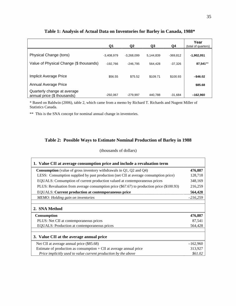
The two approaches can yield very different results. This is illustrated by the example in

table 1, which is simplified by the use of quarterly data instead of monthly data. Summing the

quarterly nominal CII estimates in second row of table 1 implies that inventory investment is

positive for the year at $87.5 million, yet in the top row of the table the year was characterized

by net withdrawals from inventories, resulting in a fall in stocks of 1.9 million tons. Valuing the

quantity change at a negative price (as is done when nominal CII for the year differs in sign from

the quantity change) is certainly paradoxical, and if the focus were on inventories in isolation, it

could potentially be misleading.

Nevertheless, in a context of the national accounts, the objective is to measure production,

as summarized by GDP. When current period production of a good exceeds consumption, the

excess production is added to inventories, while if consumption is greater than current

production, the excess consumption is supplied by a draw down of inventories. Consequently, in

4

the expenditure approach to GDP measurement, production is estimated as final purchases of

domestically produced goods and services plus CII.

Production is not only supposed to be recorded at the time that it occurs. It is also

supposed to be valued at the price that exists at that time. This is consistent with the principle in

national income accounting that holding gains and losses are included neither in measures of

production nor in measures of income. Because the price that prevails when a good is produced

determines the value of its production, subsequent changes in price during the time that the good

is held in inventories are holding gains or losses.1 Nominal consumption, on the other hand, is

recorded when an item is purchased by a final consumer and is valued at the then-current price.2

To keep holding gains and losses on inventories out of a measure of production calculated

as the sum of consumption and CII, the price that exists when an inventory addition or

withdrawal occurs is used to value the addition or withdrawal (SNA93, 6.60, and Foss, et al., no

date, 41.) This is in contrast to conventional accounting, which values an item leaving inventory

at the same price that it had when it entered inventory. Consequently, in the measurement of

nominal GDP using the expenditure approach, CII has a dual role: first, it corrects for timing

differences between consumption and production; and second, it corrects for any holding gains

and losses occurring while items are held in inventories and realized when they are sold out of

inventory as part of the selling price.

The barley producers whose inventory transactions are shown in table 1 had the

misfortunate to sell off their inventories when the price was low, only to replenish them when the

price was high. Selling when prices are low generates holding losses, and we must remove these

1 United Nations 1993 System of National Accounts (SNA93), paragraphs 6.58-6.59. 2 In the national accounts of the US, the mark-up over direct production costs included in the price received is recorded as additional production at the time of sale because inventories are valued at cost of production. The question of whether inventory valuation should include the projected mark-up over direct costs of production is not part of the inventory measurement problem that is the focus of this paper.

5

holding losses from the recorded sales of the barley producers before we can value their

production properly. The correct value of production for our purposes is shown in the Q3

column of table 1 as 564 million dollars. We omit from our illustration any production that was

immediately sold rather than added to inventories because we have no information on it.

One of the possible decompositions of the difference between current consumption (i.e.

sales) and current production is shown in the top panel of table 2. The quantity of consumption

exceeds current year production, so the first step is to exclude an estimate of consumption

supplied by production in prior years. A simple proportional split of consumption between

current year and prior year production implies that 348 million dollars of consumption were

supplied from current production. The price in the quarter when additions to stocks show that

production occurred was $109.71. In contrast, the weighted average of prices at which

inventories were sold was $67.67. The difference between these prices implies a holding loss of

216 million dollars. Adding this holding loss to consumption of 348 million dollars gives the

value of current year production at contemporaneous prices, 564 million dollars.

Provided that annual CII is defined as the sum of the four quarterly CIIs, we can arrive at

the same estimate of nominal current production for the year directly by simply adding CII for

the year to consumption expenditures—see the second panel of table 2. In contrast, valuing CII

at the average annual price would cause the current year’s production to be valued at an

implausibly low price, as shown in the bottom panel of table 2. Despite the lack of intuitive

appeal of the results for the data of table 1, we can identify the SNA93 definition of annual CII

as the one that yields the correct measure of current production.

6

B. A Procedure Suited for a World with Imperfect Data

Despite the inconvenience of discrepancies between nominal CII and the product of the

annual price and the annual change in inventory quantities, a definition of annual nominal CII as

the sum of the monthly (or quarterly) CIIs would be justifiable as necessary for accurate

valuation of current production if we lived in a Platonic world of perfect data. In practice,

however, measures of change in inventories are derived from sampled respondents’ estimates of

opening and closing stocks, each reflecting a varying mix of prices whose composition must be

inferred. Both sampling and non-sampling errors are likely in estimates derived in this manner.

Moreover, let us consider more carefully the example of table 1. We had no qualms about

valuing the years’ production at the Q3 price of $109.71 despite the fact that the average

purchaser’s price was $67.67, but perhaps we should have. For one thing, in deciding when the

production occurred, we failed to consider work-in-progress inventories. They would have

revealed that production was not really confined to Q3, so an average of the Q3 price and the Q2

price of $75.52, or $92.62, would be appropriate for valuing the production. Indeed, one could

arguably view the production of barley as an annual cycle process, and value the 1988

production at the average price for the year of $85.68.

It seems imprudent to accept large adjustments for holding gains and losses on inventories

based on monthly data that are subject to stochastic errors and possible incompleteness, while

small adjustments that could be wrong do not seem worth the inconvenience that they cause.

The idea of adjusting estimates subject to stochastic errors in the direction of zero has some

resemblance to Bayesian shrinkage estimators, which shrink the estimates in the direction of a

prior of zero, reducing their variance and their mean squared error (MSE). Indeed, the SNA93

7

itself concedes—albeit in a paragraph (6.68) that contains two warnings—that data limitations

may make “approximate” measures of annual CII more practical than the theoretically ideal one.

Our proposed solution to the problem of measuring inventory change at the item level is a

procedure for benchmarking monthly estimates of CII to annual control totals. Measures of non-

farm CII in the US national accounts are based on large mandatory surveys at annual frequencies

and on smaller voluntary surveys at monthly frequencies. Besides the extra accuracy conferred

by the larger sample size of the annual survey, respondents tend to be more careful about the

methods used for inventory valuation at year end than they are at other times.

Annual benchmarking is a way to take advantage of the greater reliability of the annual

survey data. Once the year is over and measures of annual inventory change have been

estimated from the annual survey of inventory stocks, the annual estimates are used to

benchmark the original monthly estimates of inventory change.

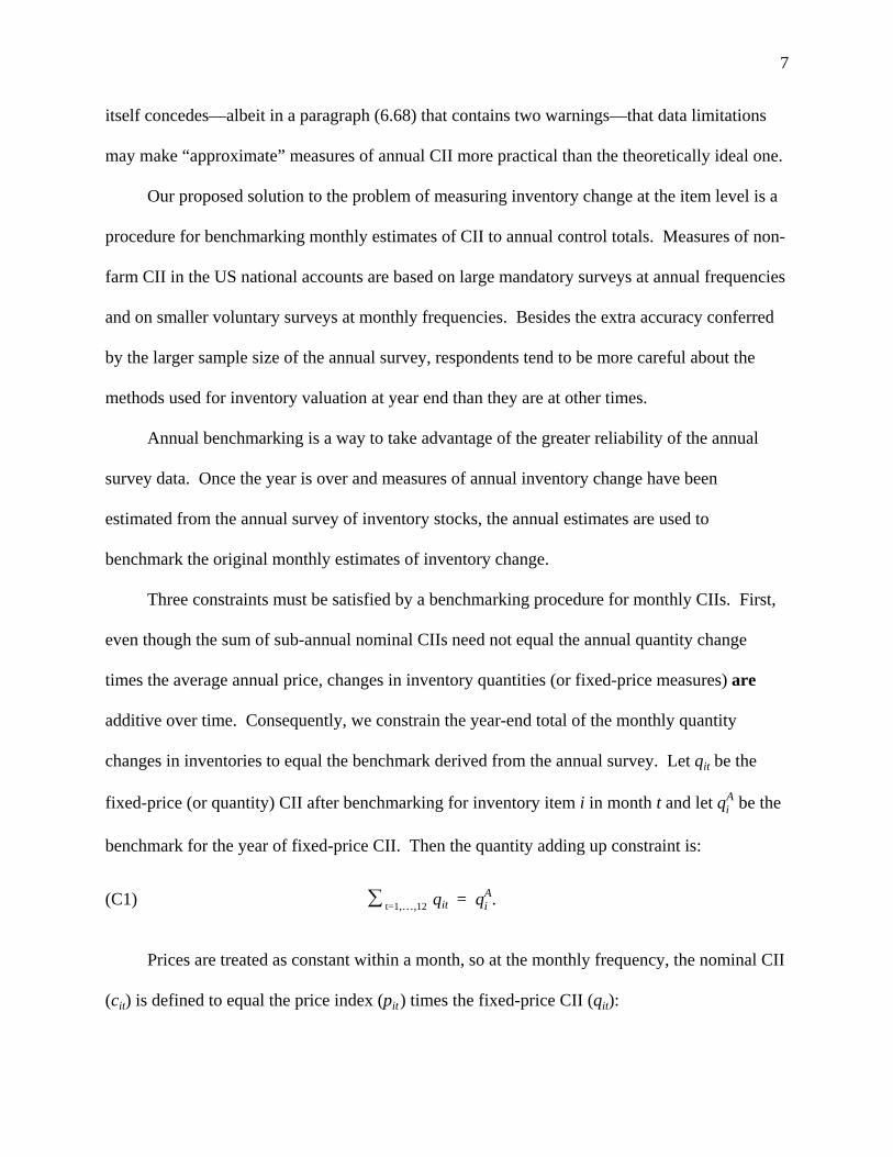
Three constraints must be satisfied by a benchmarking procedure for monthly CIIs. First,

even though the sum of sub-annual nominal CIIs need not equal the annual quantity change

times the average annual price, changes in inventory quantities (or fixed-price measures) are

additive over time. Consequently, we constrain the year-end total of the monthly quantity

changes in inventories to equal the benchmark derived from the annual survey. Let qit be the

fixed-price (or quantity) CII after benchmarking for inventory item i in month t and let qAi be the

benchmark for the year of fixed-price CII. Then the quantity adding up constraint is:

(C1) ∑ t=1,…,12 qit = qAi .

Prices are treated as constant within a month, so at the monthly frequency, the nominal CII

(cit) is defined to equal the price index (pit) times the fixed-price CII (qit):

8

(1) cit ≡ pitqit i = 1,2,…,12.

The nominal CIIs are used in our second constraint, which follows the conceptual treatment of

inventories in the SNA93. This constraint requires that the annual measure of nominal CII equal

the sum of the monthly nominal CIIs:

(C2) cAi = ∑ t=1,…,12 cit .

Third, because no obvious weighting scheme exists for averaging monthly prices, we

constrain the annual price index to be the simple average of the monthly price indexes:

(C3) −pi = 112 ∑ t=1,…,12 pit .

A constraint that could be impossible to satisfy exactly may be maintained as an objective.

One such objective is consistency between the annual price, the annual fixed-price CII, and the

annual nominal CII, meaning that the implicit price index calculated as the ratio of nominal

annual CII to fixed-priced annual CII equals the explicitly calculated annual price index:

(O1) cAi = −pi q

Ai .

Imagine for expositional purposes that we begin with estimates of the qit and the pit and

solve for three unknowns, qAi , c

Ai and −pi. The solution to the system of three equations

represented by (C1), (C2) and (C3) is generally unlikely to satisfy the fourth equation (O1).

Alternatively, if we start with the benchmark estimates of qAi and cA

i , then make uniform

adjustments to original estimates of the qit to get them to add up to qAi and, finally, solve for

revised cit via equation (1), we are likely to violate equation (2). Other simple schemes will also

lead to frequent violations of one of the four equations.

9

In the benchmarking process we must adjust the qit to values that add up to qAi , but we

need not make the same adjustment in every month. Regarding our system of four equations as

one in twelve unknowns, rather than three unknowns, transforms the solution set from being

empty to containing an infinite number of points. To choose among these points, we solve a

minimization problem that embodies another objective: the preservation of information on the

intra-year pattern of economic activity and on holding gains and losses. This means that we

want the benchmarked monthly fixed-dollar CIIs to have the same pattern over the year as the

original estimates of the monthly CIIs derived from the monthly survey data, denoted by qMit .

We cannot simply impose a binding constraint on the monthly pattern of the benchmarked

estimates because doing so would effectively bring us back to a situation where we have four

equations in three unknowns, with the likely result of large violations of objective (O1). One

reason why objective (O1) is important is that the annual measure of real GDP becomes more

consistent with the measure of nominal GDP when the same price and quantity data are used to

calculate both measures. In particular, if (O1) is always satisfied, there will be no need to choose

between discrepant direct and implicit price indexes for GDP.3 Second, when (O1) is severely

violated—as was the case in the example of table 1—our transformation of an industries’ sales

(i.e. the consumption of its output) into an estimate of its current production by adding CII

incorporates an uncomfortably large adjustment to the price actually realized.

In most cases the intra-year data on inventory change are subject to sampling error and to

response error, and the associated prices are also imperfectly measured. We should, therefore,

proceed cautiously when adjusting the well-measured consumption value of a good to a quite

3 Agreement between the direct and implicit price indexes is the most celebrated property of the Fisher index formula used by BEA, but this property requires that the data used in the quantity index be consistent with the data used in the price index. Violations of (O1) by the annual data on change in inventories account for the discrepancy between the published Fisher price index for GDP and the GDP implicit price deflator in the US national accounts.

10

different estimate of its value in production on the basis of possibly mismeasured data. This is

especially so because the inconvenience of gaps between these two values makes our “loss

function” asymmetric: an overestimation of the absolute size of this gap is less acceptable than

an underestimation. Given these considerations, a desire to take a conservative approach to

imputing holding gains or losses on inventories justifies the use of a procedure that adjusts the

estimate implied by the raw data to zero if the estimate from the raw data is small, or in the

direction of zero if the estimate from the raw data is large.

The solution that implies zero holding gains on inventories is obtained when we impose

equation (O1) as a fourth constraint. The Lagrangian for the problem of minimizing the sum of

squared differences between the benchmarked monthly estimates qit and the unadjusted estimates

qMit subject to (1) the adding-up constraint (C1), and (2) a constraint implied by equation (O1) is:

(2) minqi1‚…‚qi‚12

∑ t (qMit – qit)

2 + λ1{[∑ t qit] – qAi } + λ2{ −pi[∑ t qit] – ∑ t pit qit}.

One way to satisfy the two constraints included in equation (2) is to take advantage of the

orthogonality condition X′ $e = 0 that is a key property of the residuals $e from regression on

explanatory variables X. This means that the twelve residuals $eit from a regression of the qMit on

the pit and an intercept will sum to zero regardless of whether they are interacted with the pit .

This suggests that we might calculate qit as $eit plus a constant, where $eit = qit – − Μqi + $βi(pit – −pi ):

(3) qit = 112qA

i + $eit. t = 1,2,…,12

But is equation (3) the optimal solution for the qit? The following proposition answers this

question affirmatively.

11

Proposition 1: The solution to the minimization problem of equation (2) consists of the

sums of residuals from a regression of the qMit on the pit and a constant, as shown in equation (3).

Proof: Differentiating equation (2) with respect to the qit shows that:

(4) qit = qMit + λ1/2 + (λ2/2)(pit – −pi) t = 1,2,…,12.

Equation (4) shows that a change in λ1 affects each of the qit by the same constant amount.

In particular, replacing qAi inside the λ1 constraint in equation (2) by 0 will change only the value

of λ1, so after we adjust it by adding the appropriate constant (its value is 112qA

i ), the solution for

qit from an alternative problem where the qit are constrained to add up to 0 is the same as the

solution equation (2). Therefore, provided that we remember to add the constant 112qA

i to the

solution vector, we can treat the problem in equation (2) as equivalent to a problem where the

objective is to minimize (y–$e)′(y–$e) subject to the constraints given by the rows of the equation

X′ $e = 0, where y is the vector of the qMit , and X is an explanatory variable matrix with 1s in its

first column and the pit in its second column. Substituting in the definition for $y implicit in the

identity y ≡ $y + $e, we can rewrite this objective as one of minimizing the “regression sum of

squares” $y′ $y subject to X′ $y = X′y. Letting X1t = 1 for all t to reflect presence of 1s in first

column of X and letting X have K columns for the sake of generality, the solution is found by

minimizing the Lagrangian containing the constraints given by the rows of X′ $y = X′y:

(5) min $y1‚…‚

$yT

∑ t $yt2 + λ1[∑ t (yt – $yt)] + λ2[∑ t X2t(yt – $yt)] + … + λΚ[∑ t XKt(yt – $yt)]

12

The derivatives of this Lagrangian with respect to the $yt imply that each $yt is the same

linear function of the explanatory variables (specifically, the function whose coefficients are

λ1/2, λ2/2,…,λK/2.) Denoting the vector of these coefficients by $β, substitute X $β for $y in the

constraint X′ $y = X′y and solve for $β. This yields the standard regression formula of $β =

(X′X)–1X′y, which establishes that the $e that solves our minimization problem is indeed the

standard regression residual vector.

Equation (3) is quite satisfactory as an estimator for the fixed-price monthly inventory

change when R2 from the regression of the qMit on the pit is not large: in this case, the

benchmarked monthly CIIs will have a pattern over the year that closely mimics the original

monthly CIIs. (For convenience, we omit the i subscript on R2 even though it obviously varies

across items.) If, on the other hand, the regression’s R2 is near 1, the residuals will be near zero

and the qit will preserve little of the original pattern of the qMit . The undesirability of high R2s

makes our problem quite unlike the usual applications of the regression technique, where the

research hopes for a high R2.

If the monthly data strongly suggest the presence of significant holding gains or losses on

inventories and of large differences between months in net inventory investment, these patterns

are unlikely to arise entirely from incomplete or inaccurate data. Under this circumstance,

therefore, the annual estimate of nominal CII should provide for the presence in the consumption

data of some holding gains or losses the need to be kept out of the measure of output.

To make sure that most of the original pattern of the monthly quantities is retained after

benchmarking in cases when R2 is high, in these cases we include a damping factor k that moves

13

$βi in the direction of zero. Let R2* denote the maximum allowed for the proportion of the

variance of the original monthly CIIs removed in benchmarking. This is equivalent to requiring

that the benchmarked monthly CIIs preserve enough of the variation originally present to have a

variance equal to at least 1– R2* times the original variance. In the appendix we show that to

achieve this, the damping factor should be calculated as:

(6) k = 1 – [1 – R2*/R2]1/2

if R2 > R2*. Letting k = 1 if R2 ≤ R2* and letting $β i be the regression slope coefficient on the pit,

the generalized expression for the residual is:

(7) %εit = qM

it – [ − Μqi + k $β i(pit – −pi) ].

The benchmarked fixed-dollar monthly CIIs that include the damping factor are defined as

(8) %qit = %εit + qAi /12. t = 1,2,…,12.

Note that ∑ t %qit = qAi , so constraint (C1) is still satisfied. However, for R2 > R2*, the

benchmarked estimate of current-dollar annual CII no longer equals −piqAi . Substituting the

formula for the regression slope coefficient Cov(p i ,qi)/Var(p i ) for $β i2 in the equation for %εit

shows that ∑ t pit %εit = (1 – k)Cov(p i ,qi), so:

(9) ∑ t pit %qit = (1 – k)Cov(p i ,qi) + −pi qAi .

Assuming that the monthly inventory change data are perfectly measured, the value of the

holding gains embedded in the annual sales figures for item i is –Cov(p i ,qi) and annual current-

dollar output of item i equals its annual consumption plus net investment in inventories measured

14

as Cov(p i ,qi) + −piqAi . Therefore k equals the proportion of the holding gains on inventories

implied by the monthly data that is not removed from the benchmarked annual measure of

output when nominal net investment in inventories for the year is measured by equation (8).

In practice, we set R2* equal to 0.333, so that at least two-thirds of the variance in the

original fixed-dollar monthly CIIs is always preserved. Under the null hypothesis of no

systematic relationship between prices and quantities, we can expect to see R2 ≤ 0.333 about 95

percent of the time assuming normally distributed errors.

C. Problem caused by Requiring Nominal GDP to Equal Real GDP in the Base Year

The convention of setting nominal GDP equal to fixed-price or real GDP in the base year

is usually viewed as an innocent, mathematically trivial normalization. This would indeed be

true had we defined the annual nominal measure of inventory change for a detailed item as a

reflated fixed-price measure. As that is not the case, to obtain equality in the base year between

components of nominal GDP and corresponding components of real GDP, we must choose

between a distortion in the base year estimate of nominal GDP and a distortion in the estimate of

the change in real GDP. Our one consolation in making this unpleasant choice is that neither

distortion is likely to be numerically important.

The genesis of the problem is the use of the measure of nominal CII to adjust for the

holding gains and losses on inventory items that do not belong in the measure of production. For

non-inventory items, the annual price can be calculated as a unit value (i.e. a quantity-weighted

average), ensuring equality between the nominal expenditure for the year and the product of the

annual price and the annual quantity. In contrast, for inventory items, no quantity weights are

available, so a simple average of monthly prices must be used. Consequently, the product of the

15

annual price and the annual quantity fails to equal the annual nominal CII in cases where k < 1,

as shown in equation (9).

At least a few such cases are likely to occur in the base year. In these cases, to obtain

identical measures of nominal and fixed-price CII, we must either adjust the measure of nominal

CII or the measure of fixed-price CII. If we choose the former strategy, making the measure of

nominal CII equal to qAi , the measure of nominal GDP in the base year will be distorted. In

effect, the wrong price will be used to value production. For example, with the data of table 1,

barley production would be valued at $61.02 per ton, far below the range of theoretically

defensible prices of $92.61 to $109.71.

If, on the other hand, we adjust the estimate of fixed-price annual CII to make it equal to

the nominal annual CII of ∑ t pit %qit , the inclusion of holding gains and losses in the measure of

fixed-price CII in the base year will distortion the estimates of change in real CII. For example,

given the data in table 1, the estimator for nominal annual CII on the left side of equation (9)

would imply an adjusted estimate of fixed-price CII of about +$5 million, so that the negative

physical change in inventory stocks was valued at negative price. Furthermore, if the measure of

fixed-price inventory stocks is built up by cumulating fixed-price inventory investment (as is the

case in the NIPAs) the estimates of fixed-price stocks will also be distorted if the base year

estimate of fixed-price investment is adjusted to equal the nominal investment.

The distortion in the estimate of nominal GDP is more acceptable than the one in the

estimated growth of real GDP, so in the base year we require that nominal CII always equal qAi ,

where the units of measurement for qAi are such that −pi = 1 in the base year. This could easily be

accomplished by letting k equal 1 in equation (7) even when R2 is high, but the result would be to

compound the error by introducing a second distortion, an excessive smoothing of the intra-year

16

pattern of CII. (A regression R2 near 1 implies that the residuals are near zero, so when we use

these residuals to benchmark the months, any pattern present in the monthly data will be revised

to a flat line.) We therefore calculate k in the usual manner in the base year, letting it be small

when R2 is large. We then eliminate the discrepancy that occurs in these cases between qAi (the

benchmark value of CII for base year given that in that year −pi ≡1) and ∑ t pit %qit by distributing it

over the months in proportion to the absolute values of the monthly CIIs. This minimizes the

distortion to the relative magnitude of the monthly nominal CIIs (i.e. the pit %qit). In the base year

the monthly nominal CII for item i is calculated as:

(10) %cit = pit %qit + | pit %qit |

∑ s | pis %qis | [qA

i – ∑ s pis %qis].

For items with k < 1 in the base year, the second term on the right side of equation (10) will

be non-zero. As a result, the monthly nominal CII will no longer equal the product of the

monthly price and the monthly fixed-price CII. The monthly counterpart of constraint (C1) is

then violated in order to preserve information on the intra-year pattern of the CII in the base year

that would otherwise be lost.

D. Empirical Tests of the Benchmarking Method

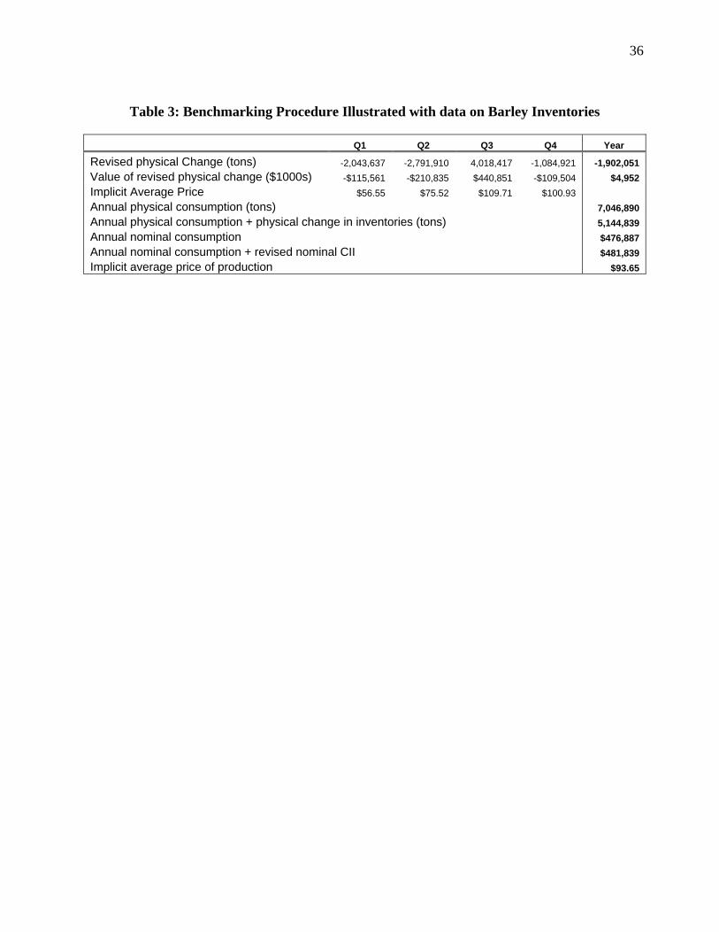
We begin our empirical tests of the methods proposed above with the Canadian barley data

of table 1. Although the example was not one of benchmarking to a predetermined annual total,

for illustrative purposes we assume that there was an annual benchmark equal to the actual

annual total of -1,902,051 tons.

Not surprisingly, in the case of the data in table 1, R2 from the regression of quantities on

prices is quite high, with a value of 0.742. Our damping factor k from equation (6) therefore

17

equals 0.33. This leads to relatively modest revisions of the unadjusted quantity data, as is seen

in figure 1. The revised quantities imply revised nominal CIIs for the four quarters that yield a

downward revision of the estimate of nominal annual CII from $87,541 to $4,952—see table 3.

The implied nominal measure of annual production has the same downward revision. The

revised price that is implicitly being used to value the production may be found by dividing the

revised nominal measure of production of $481,839,000 by the quantity of production of

5,144,939 tons, resulting in a price of $93.65. This is quite close to the average of the Q2 and

Q3 prices of $92.61, which above we found to be more reasonable than price of $109.71 that is

implied by unadjusted annual measure of nominal CII. Thus, equation (8) seems to perform

satisfactorily when confronted with the Canadian barley data.

Figure 1: Adjusted Quantity Change for Example of Barley in Canada in 1988

-4,000,000

-3,000,000

-2,000,000

-1,000,000

0

1,000,000

2,000,000

3,000,000

4,000,000

5,000,000

6,000,000

1 2 3 4

Quarter

tons

Quantity change afteradjustment

Quantity change inoriginal data

We also conducted extensive empirical tests of the equation (8) method using U.S. national

income and product accounts (NIPA) data for the time period 1997 to 2005. For this time

period, the NIPA data on changes in inventory are calculated on an industry basis using the

18

North American Industry Classification System (NAICS). Annual estimates of change in

inventory are calculated for 568 industries (417 industries starting in 2002). Of those industries,

473 represent the manufacturing sector (322 industries starting in 2002). Each manufacturing

industry comprises three subcategories, one for each stage of fabrication (materials and supplies,

work-in-progress, and finished goods). Therefore, a total of 1,514 individual industry series

have to be benchmarked each year.

Equation (8) is not currently used by BEA, so in the tests we were interested in both the

revisions to the unadjusted data and how the series that were adjusted using equation (8)

Figure 2: Quarterly Current-Dollar Changes in Inventory, Item no. CBI_Nonfarm

-100000

-50000

0

50000

100000

150000

97 Q1 97 Q4 98 Q3 99 Q2 00 Q1 00 Q4 01 Q3 02 Q2 03 Q1 03 Q4 04 Q3 05 Q2

Mill

ions

of C

urre

nt D

olla

rs

Current method

Adjusted

19

compared to those calculated using the current method. (The currently used method achieves

satisfaction of constraint (O1) by adding the necessary constant to each of the unadjusted

monthly measures of nominal CII.)

A modest reduction in volatility in the estimate of aggregate current-dollar changes in

nonfarm inventory when equation (8) is used is evident in figure 2, which charts the results. In

general, though, the two methods yield similar results. One likely cause of the similar results is

that the correlation between monthly prices and monthly fixed-price CIIs is low in most cases.

In cases with an R2 of 0.333 or less, we are able to satisfy all the constraints by setting k

equal to 1 in equation (7). An example of an industry where all constraints were always satisfied

is merchant wholesale motor vehicles (item no. cbi4211), shown in figure 3. However in one

year, 2001, R2 for this industry was a bit high at 0.21 and the annual benchmark implied the need

for a substantial upward revision in the average level of the monthly estimates. The price index

fell sharply in the fourth quarter, so that is where equation (8) concentrated the revision.

Figure 3: Monthly Current-Dollar Changes in Inventory, Item no. cbi4211

-1000

-500

0

500

1000

1500

Jan-00 May-00 Sep-00 Jan-01 May-01 Sep-01 Jan-02 May-02 Sep-02 Jan-03 May-03 Sep-03

Mill

ions

of C

urre

nt D

olla

rs

Current method

Adjusted

Unadjusted

20

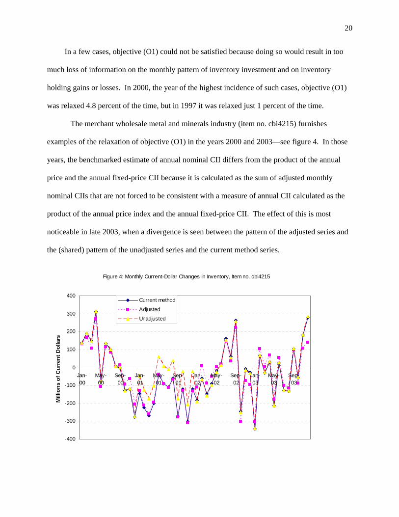
In a few cases, objective (O1) could not be satisfied because doing so would result in too

much loss of information on the monthly pattern of inventory investment and on inventory

holding gains or losses. In 2000, the year of the highest incidence of such cases, objective (O1)

was relaxed 4.8 percent of the time, but in 1997 it was relaxed just 1 percent of the time.

The merchant wholesale metal and minerals industry (item no. cbi4215) furnishes

examples of the relaxation of objective (O1) in the years 2000 and 2003—see figure 4. In those

years, the benchmarked estimate of annual nominal CII differs from the product of the annual

price and the annual fixed-price CII because it is calculated as the sum of adjusted monthly

nominal CIIs that are not forced to be consistent with a measure of annual CII calculated as the

product of the annual price index and the annual fixed-price CII. The effect of this is most

noticeable in late 2003, when a divergence is seen between the pattern of the adjusted series and

the (shared) pattern of the unadjusted series and the current method series.

Figure 4: Monthly Current-Dollar Changes in Inventory, Item no. cbi4215

-400

-300

-200

-100

0

100

200

300

400

Jan-00

May-00

Sep-00

Jan-01

May-01

Sep-01

Jan-02

May-02

Sep-02

Jan-03

May-03

Sep-03

Mill

ions

of C

urre

nt D

olla

rs

Current method

Adjusted

Unadjusted

21

III. Measuring Real Change in Inventories in a Fisher Index Framework

We now shift our focus from the measurement of CII for a single item to the measurement

of aggregate CII and from the measurement of nominal values to the measurement of real values.

Once the question of how to form nominal measures of CII for individual items has been settled,

aggregating them is a trivial matter. In contrast, designing an aggregate measure of real CII is a

difficult problem. A Laspeyres or Paasche index calculated in the usual way from CII data may

have a numerator that differs in sign from its denominator, or a denominator that is near zero.

Under these circumstances, standard index numbers lose their meaningfulness, suggesting that

the attempt to measure aggregate real CII is futile (Diewert, 2004, 2005.)

Yet even if it were true that a meaningful measure of real CII can sometimes fail to exist,

that would not be a reason to deprive users of the national accounts of information that is

generally useful by dropping real CII from the published set of economic indicators. We

therefore seek a solution to the problem of measuring real CII that is applicable under the

broadest possible range of circumstances.

In the NIPAs, the solution to the need to avoid indexes of inventory flows has been to

calculate real CII as the first difference of real inventory stocks. This procedure uses stocks as

weights for flows, ignoring the fact that the composition of the stocks may differ greatly from the

composition of the inventory flows. A theoretically superior procedure for estimating real CII

that subtracts real gross disposals from real gross inventory acquisitions was, therefore,

developed by Ehemann (2005). That method is quite data-intensive, however, and data on gross

flows into and out of stocks may even be unavailable in some cases. Hence, we seek a method

of measuring real CII that avoids the need for separate data on inventory gross flows.

22

A. Inventories in the Calculation of the Fisher Index Measure of Real GDP

In the base period, assumed to be period t–1, real GDP is set equal to current-dollar GDP.

In subsequent time periods, the chain Fisher index measure of real GDP in any time period s

after the base period is constructed by multiplying the previous value of real GDP by the Fisher

quantity index from period s–1 to period s. In time periods preceding the base period, real GDP

is measured by dividing by a Fisher quantity, starting with the one from period t–2 to period t–1.

The procedure can be illustrated by the first link in the forward chain, beginning with a

simplifying assumption that all inventory changes equal zero. Let pf ct q

f ct represent the current-

price final consumption of commodity c, and let pfc,t-1q f

ct represent the value of these

expenditures deflated to period t–1. With no changes in inventories, nominal GDP in period t

equals ∑ c pfct q

f ct . The Fisher quantity index of final demand, F ft , is:

(11) F ft = ⎡⎢⎣

∑ c p f ct-1 qf

ct

∑ c p f ct-1 qf ct-1

∑ c p f

ct q f ct

∑ c p f ct qf ct-1

⎤⎥⎦

0.5

,

Real GDP measured in chain-dollars of period t–1 would equal (pf t -1⋅q

f t -1) F ft.

To bring changes in inventories into the calculation of real GDP, let qit be the value in

prices of base period b of the net additions to inventories of inventory item i. Although the

period length here is a year, it is convenient to change the notation for the price index from −pi to

PAit, where PAit is the price index appropriate for deflating the flows (which are effectively

assumed to occur at uniform rate) during period t. Nominal net investment in inventory in period

t is, then, ∑ i PAit qit , or PAt⋅qt. Nominal GDP in period t is N t GDP = ∑ c p

fct q

f ct + ∑ i PAit qit . Real

GDP in dollars of period t–1, denoted Q t GDP, is:

23

(12) Q t GDP = Nt-1

GDP [ pf t -1⋅q

f t + PAt-1⋅qt

pf t -1⋅qf

t -1 + PAt-1⋅qt-1

pf t ⋅q

f t + PAt⋅qt

pf t ⋅q

f t -1 + PAt⋅qt-1

]0.5.

None of terms in equation (12) can be identified as a measure of real CII; the four terms

containing CII are just deflated (or reflated) measures of fixed-price CII in period t or period t–1.

The reason to estimate real CII is, then, to have a statistic that summarizes the inventory quantity

changes occurring in the economy, not to have a building block for calculating real GDP.

Nonetheless, we would like our measure of real CII to be sufficiently related to the measure of

real GDP so that it reflects the influence on real GDP of inventory investment.4 This influence

depends on the value of the change in CII between times t–1 and t at prices of time t–1 and of

time t. In particular, if final purchases are constant, the difference between the numerator and

denominator of the quantity index for GDP equals PAt-1⋅ (qt – qt-1) in the Laspeyres case, and

PAt⋅ (qt – qt-1) in the Paasche case. This suggests that difference equations may be a promising

alternative to the unusable index number methods.

B. The Method of First-Differencing Stocks

In the NIPAs, the fixed-dollar stock of any inventory item i is calculated by accumulating

fixed-dollar inventory changes. Thus, the value of this stock at the end of period t, denoted by

kit, equals ki,t-1 + qit. The aggregate fixed-dollar stock at the end of period t–1 equals ∑ i ki,t-1.

The current-dollar stock of inventories at the end of period t–1 is measured using end-of-period

price indexes PKit, where PKit is related to PAit by the equation PAit = 12(PKi,t-1 + PKit). The

4 The objective of reflecting the role of inventory investment in real GDP may mean that we must forego another objective, measuring the evolution of the aggregate real stocks.

24

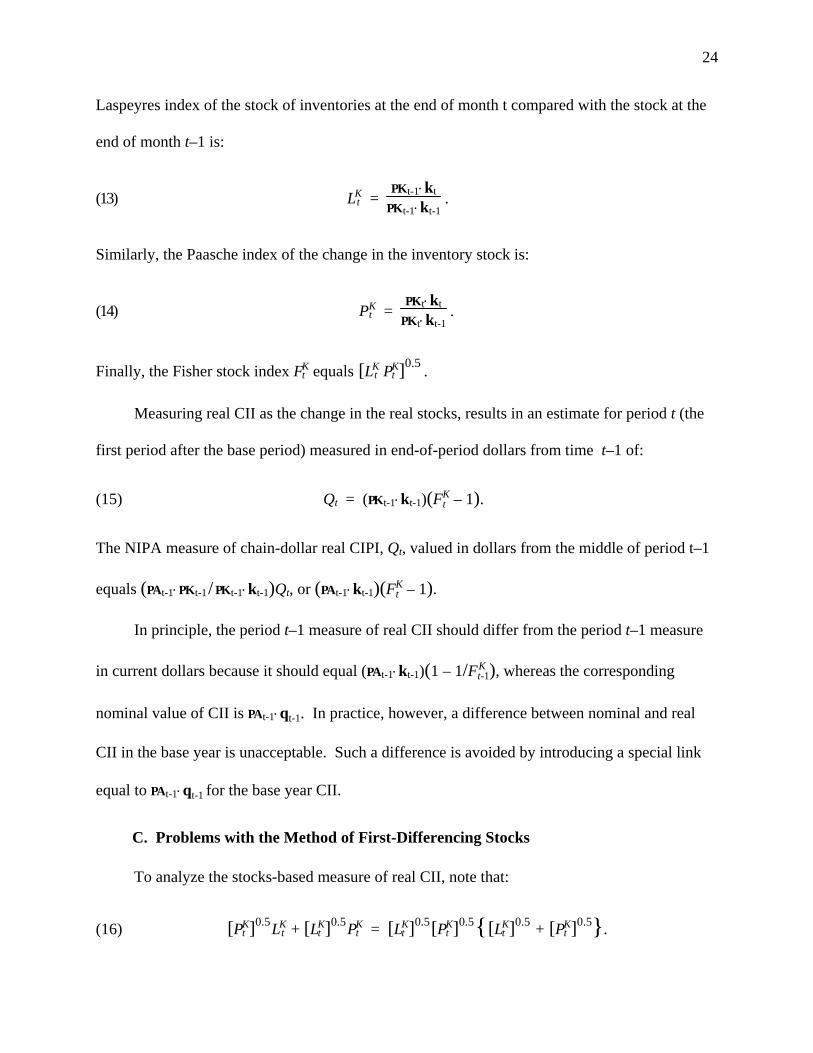
Laspeyres index of the stock of inventories at the end of month t compared with the stock at the

end of month t–1 is:

(13) LKt =

PKt-1⋅kt

PKt-1⋅kt-1 .

Similarly, the Paasche index of the change in the inventory stock is:

(14) PKt =

PKt⋅kt

PKt⋅kt-1 .

Finally, the Fisher stock index FKt equals [LK

t PKt ]0.5 .

Measuring real CII as the change in the real stocks, results in an estimate for period t (the

first period after the base period) measured in end-of-period dollars from time t–1 of:

(15) Qt = (PKt-1⋅kt-1)(FKt – 1).

The NIPA measure of chain-dollar real CIPI, Qt, valued in dollars from the middle of period t–1

equals (PAt-1⋅PKt-1/ PKt-1⋅kt-1)Qt, or (PAt-1⋅kt-1)(FKt – 1).

In principle, the period t–1 measure of real CII should differ from the period t–1 measure

in current dollars because it should equal (PAt-1⋅kt-1)(1 – 1/FK t-1), whereas the corresponding

nominal value of CII is PAt-1⋅qt-1. In practice, however, a difference between nominal and real

CII in the base year is unacceptable. Such a difference is avoided by introducing a special link

equal to PAt-1⋅qt-1 for the base year CII.

C. Problems with the Method of First-Differencing Stocks

To analyze the stocks-based measure of real CII, note that:

(16) [PKt ]0.5LK

t + [LKt ]0.5PK

t = [LKt ]0.5[PK

t ]0.5{[LKt ]0.5 + [PK

t ]0.5}.

25

Dividing both sides of the equation by the final bracketed term shows that the Fisher index is a

weighted arithmetic average of the Laspeyres and Paasche indexes, with the weight on the

Paasche index proportional to the square root of the Laspeyres index, and the weight on the

Laspeyres index proportional to the square root of the Paasche index. We can therefore express

the Fisher index as:

(17) FKt = λtLK

t + (1−λt)PKt

where

(18) λt = [PK

t ]0.5

[LKt ]0.5 + [PK

t ]0.5 .

Another way to express λt is as the ratio of the Fisher index to the sum of the Fisher and

Laspeyres indexes. It is likely to be very near 0.5 for the indexes used to measure real inventory

change, because using stocks as weights is likely to result in close agreement between the

Laspeyres index and the Paasche index.5

Let LKPt denote the Laspeyres price index that uses stocks for weights, or PKt⋅kt-1 / PKt-1⋅kt-1.

Substituting from equation (4) for FKt in equation (6), and substituting qt for kt − kt-1, after some

algebra we find that the measure of real CII is an average of fixed-dollar change in inventories

measured in period t–1 dollars, and current-dollar change in inventories deflated by the stock-

weighted Laspeyres price index:

(19) Qt = (PKt-1⋅kt-1)[FKt – 1]

= (PKt-1⋅kt-1)[λtLKt + (1−λt)PK

t – 1] 5 The weight on the Laspeyres index in equation (17) differs from 0.5 by an order of magnitude less than the proportion by which the Laspeyres index exceeds the Paasche index. For example, if the Laspeyres-to-Paasche ratio is 1.01, then the weight for the Laspeyres index is about 0.499.

26

= λt PKt-1⋅kt + (1−λt) PKt⋅kt

LKPt

– PKt-1⋅kt-1

= λt PKt-1⋅qt + (1−λt) PKt⋅kt

LKPt

– (1−λt)PKt-1⋅kt-1

= λt PKt-1⋅qt + (1−λt) PKt⋅kt

LKPt

– (1−λt)PKt⋅kt-1

LKPt

= λt PKt-1⋅qt + (1−λt) PKt⋅qt

LKPt

.

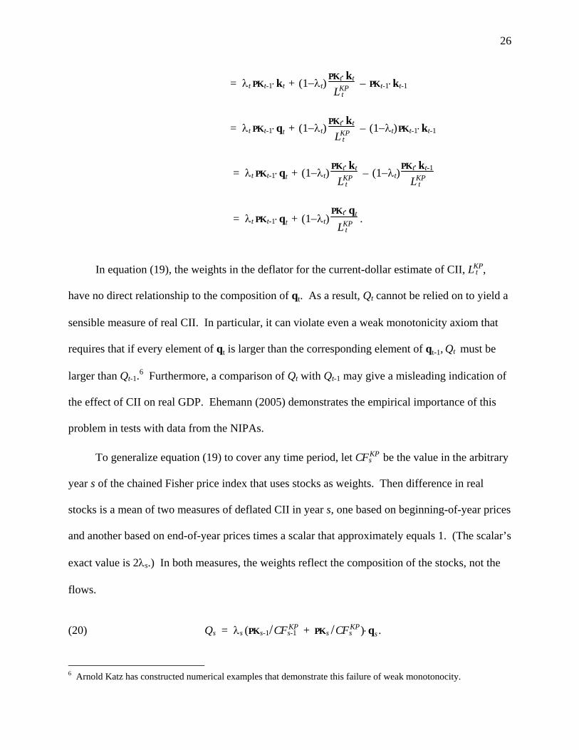
In equation (19), the weights in the deflator for the current-dollar estimate of CII, LKPt ,

have no direct relationship to the composition of qt. As a result, Qt cannot be relied on to yield a

sensible measure of real CII. In particular, it can violate even a weak monotonicity axiom that

requires that if every element of qt is larger than the corresponding element of qt-1, Qt must be

larger than Qt-1.6 Furthermore, a comparison of Qt with Qt-1 may give a misleading indication of

the effect of CII on real GDP. Ehemann (2005) demonstrates the empirical importance of this

problem in tests with data from the NIPAs.

To generalize equation (19) to cover any time period, let CFKPs be the value in the arbitrary

year s of the chained Fisher price index that uses stocks as weights. Then difference in real

stocks is a mean of two measures of deflated CII in year s, one based on beginning-of-year prices

and another based on end-of-year prices times a scalar that approximately equals 1. (The scalar’s

exact value is 2λs.) In both measures, the weights reflect the composition of the stocks, not the

flows.

(20) Qs = λs (PKs-1/CFKPs-1 + PKs /CFKP

s )⋅qs .

6 Arnold Katz has constructed numerical examples that demonstrate this failure of weak monotonocity.

27

D. An Improved Measure for Real CII

Although equation (19) appears to be an unsatisfactory way to measure real CII, its

functional form does suggest an approach that avoids an application of index number techniques

to data that are unsuitable for this purpose. That approach is based on the observation that the

value of one year’s quantity changes at its own or some other year’s prices is always a well-

defined concept, regardless of its suitability for index number construction. Thus, for example,

we ask can how much the changes in quantities from last year to this year would be worth at last

year’s prices, and also how much these changes would be worth at this year’s prices. We can

then average these two dollar-denominated measures, with just a limited reliance on a price

index for deflation purposes.

To develop a measure of real CII based on a sum of terms that measure the value of qt at

prices from periods t–1 and t, we use the axiomatic (or test) approach to index numbers as a

guide. Four axioms that the improved measure of real CII, denoted by Q∗t , should ideally satisfy

are listed below. The first three of these axioms each imply the use of the inventory flow prices

PAt, so we no longer consider the use of the inventory stock prices PKt.

Axiom I: Generalization of the ordinary measure of real values in the NIPAs. The

need for special procedures for measuring real changes in inventories arises because the changes

may not all have the same sign. However, in cases where all the values do have the same sign,

the standard Fisher measure is known to have many advantages. If all the changes in inventories

have the same sign, these advantages should not be sacrificed unnecessarily, and if the changes

are predominantly of one sign, the measure should come close to the one that has these

advantages. Therefore, if qi,t-1 ≥ 0 and qit ≥ 0 for all i, with the inequality strict for least one qi,t-1

and at least one qit, then Q∗t should equal the ordinary measure of real chain-dollar value, defined

28

as Q∗t -1F

qt , where Fq

t is the geometric mean of the Laspeyres index for flows, PAt-1⋅qt

PAt-1⋅qt-1 , and the

Paasche index for flows, PAt⋅qt

PAt⋅qt-1, and where Q∗

t -1 ≡ PAt-1⋅qt-1.

Axiom II: Approximately monotonic relationship to effect on real GDP. If qt∗ implies

a value for QtGDP that exceeds the value implied by qt by more than some small positive amount

Δ, then Q∗t should be larger when calculated with q t

∗ than when calculated with qt. A positive

tolerance Δ is necessary in this axiom because the effect of CII on real GDP partly depends on

the variables entering the calculation of real GDP but not the formula for real CII.

Axiom III: Sign agreement with any effect on real GDP of non-trivial magnitude.

The change in real CII should have the same sign as the contribution of the change in CII to real

GDP if the latter differs from 0 by a non-trivial amount. That is, the sign of the effect on real

GDP of the change from qt-1 to qt should be the same as the sign of Q∗t – Q∗

t -1 if

|Q∗t – Q∗

t -1| > Δ for some Δ > 0. Sign agreement is, of course, implied by satisfaction of the

monotonicity axiom, because in that axiom qt can equal qt-1.

Axiom IV: Homogeneity of degree 0 in final period prices. If every price PAi,t-1 is

multiplied by the same constant to obtain PAt, the structure of relative prices is unchanged and

the chain-dollar measure of real CIPI should equal the fixed-dollar measure PAt-1⋅qt. More

generally, if for some positive constant k, PA t∗ = kPAt , then the substitution of PA t

∗ for PAt in

the formula for Q∗t should have no effect on the result.

Proposition 2 introduces a Fisher-like measure of real CII that satisfies our axioms.

29

Proposition 2. Let qdst denote the vector of “dominant-sign” elements qt, where zeros

replace the negative elements of qt if PAt⋅qt ≥ 0 or the positive elements of qt if PAt⋅qt < 0. Let

Lds t equal the Laspeyres price index

PAt⋅q dst-1

PAt-1⋅q dst-1

if at least one element of qt-1 is non-zero or, if the

Laspeyres index is undefined, let Lds t equal the analogous Paasche price index

PAt⋅qdst

PAt-1⋅qdst .

Similarly, let Pds t equal the Paasche price index or, if the Paasche index is undefined, let Pds

t

equal the Laspeyres price index. If either qt and qt-1 has at least one non-zero element, μt is

defined as:

(21) μ t = [P ds

t ]0.5

[Ldst ] 0.5 + [P ds

t ]0.5 .

Otherwise, let μ t = ½. Then the real measure of real inventory change Q∗t , defined as,

(22) Q∗t = Q∗

t -1 + μ t PAt-1⋅(qt – qt-1) + (1–μ t) PAt⋅(qt – qt-1)

Lds t

,

satisfies axioms I and IV, and approximately satisfies axioms II and III.

PROOF: See appendix.

To generalize equation (22) to any time period, let CFds s be the chained Fisher index for

the arbitrary period s constructed from the dominant-sign Laspeyres and Paasche indexes. Then:

(23) Q∗s = Q∗

s -1 + μ s[PAt-1

CFds s-1

+ PAs

CFds s

] ⋅(qs – qs-1)

Assuming that period t–1 is the base period, when prices are all normalized to 1, Q∗t -1 in equation

(22) is a simple sum of fixed-price CIIs. Equation (21) measures real CII in period t in terms of

30

prices of period t–1. We can also use the difference equation (23) to estimate real CII in any

time period by cumulating changes from the base year.

As an alternative to calculating weights for the Laspeyres and Paasche price indexes by

zeroing out each qit that disagrees in sign with PAt⋅qt, and similarly for each qi,t-1 that disagrees in

sign with PAt-1⋅qt-1, we could use absolute values of the qit to weight the price index.

Figure 5 shows how the proposed measure of real CII with price index weights based on

absolute values of qt performs when applied to annual data of the sort used in the NIPAs. Figure

6 repeats the test of the proposed method using quarterly data. Despite the existence of

hypothetical examples of illogical behavior of the current measure of real CII based on the

change in Fisher stocks, the performance of this measure with actual data is similar to the

performance of the theoretically superior method that uses dominant sign flows as weights in the

deflator. Nevertheless, some downward bias in the slope of the long run trend seems to be

present in the difference-of-stocks method. Theory suggests that such a bias is to be expected:

the user cost formula for the inventory stocks implies that this cost is high when the stockpiled

item has a declining price and low when the stockpiled item has a rising price. Businesses’

desire to avoid holding losses on inventories and to benefit from holding gains may therefore

make the stock weights high for the items with the largest price increases, imparting an upward

bias to the deflator and a downward bias to the measure of real CIPI based on first differences of

real stocks.

31

Figure 5: Real Nonfarm Change in Private Inventories, Annual Data (in millions of chained 2000 dollars)

-40000

-20000

0

20000

40000

60000

80000

1997 1998 1999 2000 2001 2002 2003 2004 2005

Proposed procedure (dominant sign flows as weights in deflator)Current procedure (stocks as weights in deflator)Fixed Dollars (from 2000)

Figure 6: Real Nonfarm Change in Private Inventories,Quarterly Data (in Millions of Chained 2000 Dollars)

-80000-60000

-40000-20000

02000040000

6000080000

100000120000

1997

01

1998

01

1999

01

2000

01

2001

01

2002

01

2003

01

2004

01

2005

01

Proposed procedure (dominant sign flows as weights in deflator)

Current procedure (unadjusted Fisher stocks as weights in deflator)

32

IV. Conclusion

Procedures that are theoretically correct can work poorly in actual practice when

measurement error is present in the data. (The problem of formula bias in the US CPI, which

was caused by an attempt to implement a theoretically elegant sample of estimator of a

Laspeyres price index without taking full account of the practical difficulties in measuring

weights, is an example of this.) In the case of nominal inventory investment for a year, the

theoretically correct procedure sums the values for the months within the year even though the

inventory additions and withdrawals in those months may take place at different prices. This has

the effect of incorporating a potentially large adjustment for holding gains and losses on

inventories in the calculation of annual production as annual final purchases plus annual net

inventory investment. However, a large adjustment of this type should be avoided unless we are

certain that the data require it, and a zero adjustment is most advantageous. Moreover, given the

likelihood of at least some inaccuracy in the monthly data, we cannot hope to measure holding

gains and losses on inventories with much precision. The procedure that we develop for

measuring nominal inventory investment incorporates an adjustment of zero for these holding

gains and losses if that is not too far from the one implied by the pattern of the monthly data.

Otherwise, the adjustment is damped towards zero.

For the problem of measuring real inventory investment, the solution that is most

satisfactory in theory is to say that the presence of sign changes prevents the construction of the

index numbers necessary to define the concept. In practice, however, real inventory investment

is a valuable statistic to users of national accounts, and the data are often well-behaved enough to

make even a conventional measure of this concept informative. Suppressing this statistic is

therefore not a practical alternative. The commonly used procedure of first differencing the

33

Fisher inventory stocks is one possible solution to real inventory investment problem. Yet this

procedure can yield distorted results because it implicitly uses inventory stocks as weights in a

price index that deflates the flows. In this paper, we develop a measure of real inventory

investment based on cumulative deflated differences. Price indexes weighted by quantity flows

of the dominant sign are used to deflate the differences. A test of the method of the method

implies a similar pattern to the first difference of stocks, except for a flattening out of the

downward tilt of the long run profile. Theory suggests that this downward tilt reflects a

downward bias that is avoided by the use of flow-based weights to calculate a deflator for the

flows.

34

References

Commission of the European Communities, International Monetary Fund, Organisation for Economic Co-operation and Development, United Nations, and World Bank, 1993. System of National Accounts 1993, Brussels/Luxembourg, New York, Paris, Washington.

Diewert, W. Erwin. 2004. “Index Number Problems in the Measurement of Real net Exports and Real net Changes in Inventories.” Manuscript, Univ. of British Columbia.

Diewert, W. Erwin. 2005. “On Measuring Inventory Change in Current and Constant Dollars.” Discussion Paper No. 05-12, Department of Economics, University of British Columbia.

Ehemann, Christopher. 2005. An Alternative Estimate of Real Inventory Change for National Economic Accounts. International Journal of Production Economics 93-94, pp.101-110.

Foss, Murray F., Gary Fromm, and Irving Rottenberg. (no date.) Measurement of Business Inventories, US Dept. of Commerce Economic Research Report 3.

Hicks, John R. 1940. The Valuation of Social Income, Economica 7 (May): 105-124

Lal, Kishori. 2001. “Aggregating Sub-Annual Current Price Value of Changes inInventories to Annual Totals under Condition of Inflation—An Inherent Dilemma.” Manuscript, Statistics Canada.

United Nations, 1993. See Commission of the European Communities, et al.

35

Table 1: Analysis of Actual Data on Inventories for Barley in Canada, 1988*

Q1 Q2 Q3 Q4 Year

(total of quarters)

Physical Change (tons) -3,408,979 -3,268,099 5,144,839 -369,812 -1,902,051

Value of Physical Change ($ thousands) -192,766 -246,795 564,428 -37,326 87,541**

Implicit Average Price $56.55 $75.52 $109.71 $100.93 –$46.02

Annual Average Price $85.68

Quarterly change at average annual price ($ thousands) -292,067 -279,997 440,788 -31,684 –162,960

* Based on Baldwin (2006), table 2, which came from a memo by Richard T. Richards and Nugent Miller of Statistics Canada.

** This is the SNA concept for nominal annual change in inventories.

Table 2: Possible Ways to Estimate Nominal Production of Barley in 1988

(thousands of dollars)

1. Value CII at average consumption price and include a revaluation term

Consumption (value of gross inventory withdrawals in Q1, Q2 and Q4) 476,887 LESS: Consumption supplied by past production (net CII at average consumption price) 128,718 EQUALS: Consumption of current production valued at contemporaneous prices 348,169 PLUS: Revaluation from average consumption price ($67.67) to production price ($100.93) 216,259 EQUALS: Current production at contemporaneous price 564,428 MEMO: Holding gain on inventories –216,259

2. SNA Method Consumption 476,887 PLUS: Net CII at contemporaneous prices 87,541 EQUALS: Production at contemporaneous prices 564,428

3. Value CII at the average annual price Net CII at average annual price ($85.68) –162,960 Estimate of production as consumption + CII at average annual price 313,927 Price implicitly used to value current production by the above $61.02

36

Table 3: Benchmarking Procedure Illustrated with data on Barley Inventories

Q1 Q2 Q3 Q4 Year

Revised physical Change (tons) -2,043,637 -2,791,910 4,018,417 -1,084,921 -1,902,051 Value of revised physical change ($1000s) -$115,561 -$210,835 $440,851 -$109,504 $4,952 Implicit Average Price $56.55 $75.52 $109.71 $100.93 Annual physical consumption (tons) 7,046,890 Annual physical consumption + physical change in inventories (tons) 5,144,839 Annual nominal consumption $476,887 Annual nominal consumption + revised nominal CII $481,839 Implicit average price of production $93.65

37

Appendix

1. Derivation of Equation (6)

Let $β i denote Cov(pit,qit)

Var(pit), the regression slope coefficient. Then

%qit = q Ai /12 + qM

it – [ − Μqi + k $β i(pit – −pi) ].

The variance of %qit relative to the variance of qMit is:

Var(%qit)Var(qM

it ) = 1 – 2k $β i

2 Var(pit)Var(qM

it ) + k2 $β i

2 Var(pit)Var(qM

it )

Let 1 – R2* represent the proportion of the variance that remains after benchmarking, or the

ratio of Var(%qit) to Var(qMit ). Then:

1 – R2* = 1 – 2k $β i2 Var(pit)Var(qM

it ) + k2 $β i

2 Var(pit)Var(qM

it )

0 = R2* – 2k $β i2 Var(pit)Var(qM

it ) + k2 $β i

2 Var(pit)Var(qM

it )

From the quadratic formula we have:

k = [2 $β i2 Var(pit)Var(qM

it ) – {[2 $β i

2 Var(pit)Var(qM

it )]2

– 4 $β i2 Var(pit)Var(qM

it ) R2*}1/2]/[2 $β i

2 Var(pit)Var(qM

it ) ]

k = 1 – {1 – R2*/( $β i2 Var(pit)Var(qM

it ))}1/2

But

$β i2 Var(pit)Var(qM

it ) =

Cov(pit,qit)2

Var(pit)Var(qMit )

= R2

so,

k = 1 – {1 – R2*/R2}1/ 2.

38

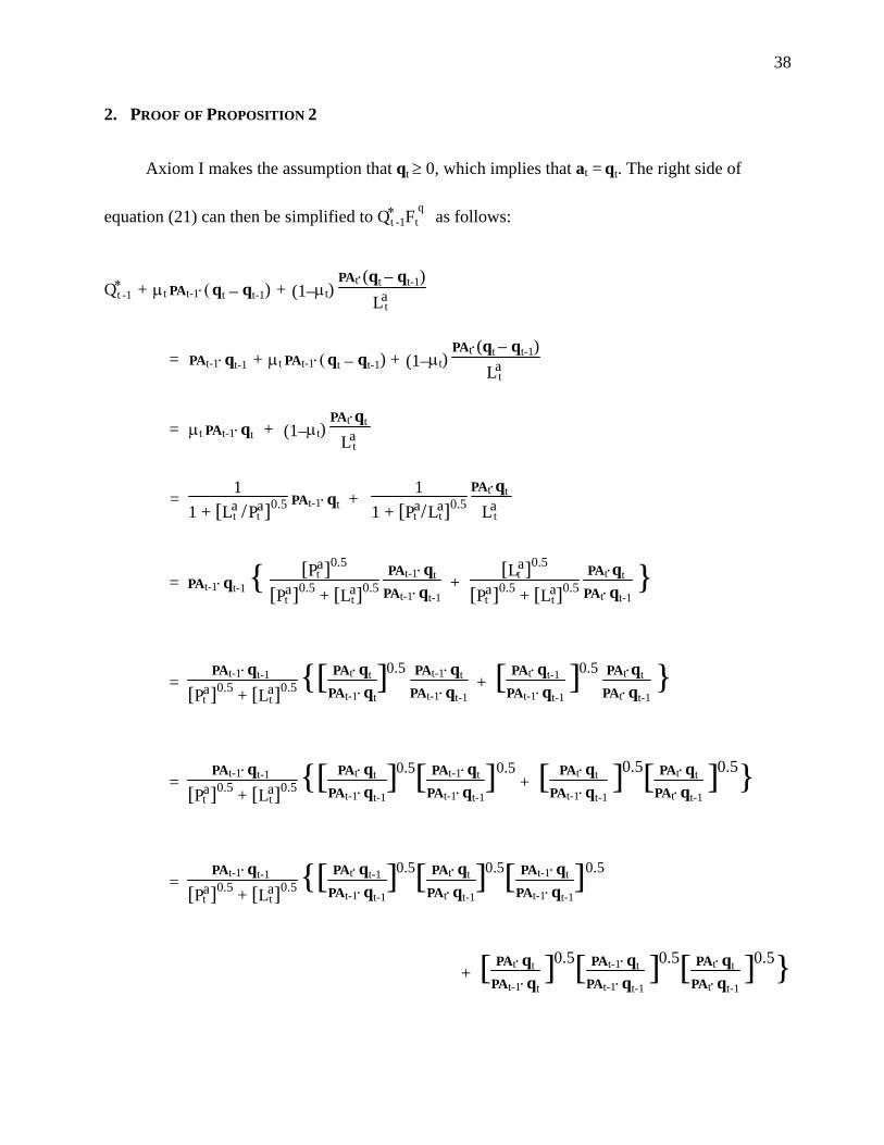
2. PROOF OF PROPOSITION 2

Axiom I makes the assumption that qt ≥ 0, which implies that at = qt. The right side of

equation (21) can then be simplified to Q∗t -1F

qt as follows:

Q∗t -1 + μt PAt-1⋅(qt – qt-1) + (1–μt)

PAt⋅(qt – qt-1)La

t

= PAt-1⋅qt-1 + μt PAt-1⋅(qt – qt-1) + (1–μt) PAt⋅(qt – qt-1)

La t

= μt PAt-1⋅qt + (1–μt) PAt⋅qt

La t

= 1

1 + [Lat /Pa

t ]0.5 PAt-1⋅qt + 1

1 + [Pat /La

t]0.5 PAt⋅qt

La t

= PAt-1⋅qt-1 { [Pa

t ]0.5

[Pat ]0.5 + [La

t]0.5 PAt-1⋅qt

PAt-1⋅qt-1 +

[Lat ]0.5

[Pat ]0.5 + [La

t]0.5 PAt⋅qt

PAt⋅qt-1 }

= PAt-1⋅qt-1

[Pat ]0.5 + [La

t]0.5 {[ PAt⋅qt

PAt-1⋅qt]0.5

PAt-1⋅qt

PAt-1⋅qt-1 + [ PAt⋅qt-1

PAt-1⋅qt-1 ]0.5

PAt⋅qt

PAt⋅qt-1 }

= PAt-1⋅qt-1

[Pat ]0.5 + [La

t]0.5 {[ PAt⋅qt

PAt-1⋅qt-1]0.5[ PAt-1⋅qt

PAt-1⋅qt-1]0.5

+ [ PAt⋅qt

PAt-1⋅qt-1 ]0.5[ PAt⋅qt

PAt⋅qt-1 ]0.5}

= PAt-1⋅qt-1

[Pat ]0.5 + [La

t]0.5 {[ PAt⋅qt-1

PAt-1⋅qt-1]0.5[ PAt⋅qt

PAt⋅qt-1]0.5[ PAt-1⋅qt

PAt-1⋅qt-1]0.5

+ [ PAt⋅qt

PAt-1⋅qt ]0.5[ PAt-1⋅qt

PAt-1⋅qt-1 ]0.5[ PAt⋅qt

PAt⋅qt-1 ]0.5}

39

= PAt-1⋅qt-1

[Pat ]0.5 + [La

t]0.5 {[Lat]0.5[ PAt⋅qt

PAt⋅qt-1]0.5[ PAt-1⋅qt

PAt-1⋅qt-1]0.5

+ [Pat ]0.5[ PAt-1⋅qt

PAt-1⋅qt-1 ]0.5[ PAt⋅qt

PAt⋅qt-1 ]0.5}

= PAt-1⋅qt-1 Fqt .

The assumption in the approximate version of axiom II is that qt′ implies a value for real

GDP that exceeds the value for real GDP implied by qt′ by at least some Δ > 0. This assumption

may be written as QtGDP′ – Qt

GDP ≥ Δ, where QtGDP′ denotes the value of equation (1) with qt′

substituted for qt. This implies that,

[ pf t -1⋅q

f t + PAt-1⋅qt′

pf t -1⋅qf

t -1 + PAt-1⋅qt-1

pf t ⋅q

f t + PAt⋅qt′

pf t ⋅q

f t -1 + PAt⋅qt-1

]0.5 – [ pf

t -1⋅qf t + PAt-1⋅qt

pf t -1⋅qf

t -1 + PAt-1⋅qt-1

pf t ⋅q

f t + PAt⋅qt

pf t ⋅q

f t -1 + PAt⋅qt-1

]0.5

≥ Δ

pf t -1⋅qf

t -1 + PAt-1⋅qt-1 . (A-1)

Let θ1 = PAt-1⋅qt′ − PAt-1⋅qt and θ2 = PAt⋅qt′ − PAt⋅qt. Let LP denote the Laspeyres price for

GDP, let LQ(qt) denote the Laspeyres quantity index for GDP evaluated at qt, and let PQ(qt) and

FQ(qt) be the analogous Paasche and Fisher indexes. Inequality (A-1) implies that θ1 and θ2 satisfy

the condition that:

[[LQ(qt) + θ1/GDPt-1][PQ(qt) + θ2 /(LPGDPt-1)]]0.5 ≥ Δ/GDPt-1 + FQ(qt) (A-2)

Squaring, and then canceling out LQ(qt)PQ(qt) on the left with [FQ(qt)]2 on the right gives:

40

θ1PQ(qt)/GDPt-1 + θ2 LQ(qt)/(GDPt-1)LP + θ1θ2 /(GDPt-1)2LP ≥ (Δ/GDPt-1)2 + 2FQ(qt)(Δ/GDPt-1) (A-3)

The terms that are divided by GDP squared are small enough to be ignored, so the

requirement that the change in CIPI raise real GDP by at least Δ is effectively a requirement that a

weighted average of θ1 and a deflated value of θ2 exceed Δ times a constant of proportionality

approximately equal to 1:

PQ(qt)

PQ(qt) + LQ(qt) θ1 +

LQ(qt)PQ(qt) + LQ(qt)

θ2 /LP ≥ 2FQ(qt)PQ(qt) + LQ(qt)

Δ. (A-4)

The expression for real CIPI in equation (9) implies that its change is also proportional to a

weighted average of θ1 and a deflated value of θ2:

Q∗t – Q∗

t -1 = [Pat ]0.5

[Pat ]0.5 + [La

t]0.5 θ1 + [La

t ]0.5

[Pat ]0.5 + [La

t]0.5 θ2 /La t . (A-5)

Solving (A-4) for θ2 as a function of θ1 and Δ, then substituting the resulting expression for

θ2 in equation (A-5) and substituting Fat for [La

t Pat ]0.5 implies:

[Q∗t – Q∗

t -1]{Fat + La

t} ≥ 2FQ(qt)L

P

LQ(qt)Δ –

PQ(qt)LP

LQ(qt) θ1 + [Fa

t ]0.5θ1 (A-6)

Substituting PP, the Paasche price index for GDP, for PQ(qt)L

P

LQ(qt) , the right side of inequality

(A-6) will be positive, implying that Q∗t – Q∗

t -1 is positive, if Δ exceeds a value that is proportional

the difference between the Paasche price index for GDP and the absolute-value weighted Fisher

price index for change in inventories:

41

Δ ≥ [PP – Fat ]

LQ(qt)2FQ(qt)L

P θ1 (A-7)

In general, the difference between the price indexes in (A-7) is likely to be small, implying

that a small positive effect of inventory change on real GDP is a sufficient condition for an

increase in real CIPI.

An approximate version of axiom III, sign agreement, follows from the approximate

satisfaction of axiom II by letting qt = qt-1.

Axiom IV is satisfied because multiplying every element of PAt by the same positive scalar

will not affect the ratio of the Laspeyres and Paasche price indexes or the deflated value of PAt,

given by PAt

La t .