LETTERSPUBLISHED ONLINE: 7 MARCH 2016 | DOI: 10.1038/NPHYS3679

How superfluid vortex knots untieDustin Kleckner1*†, Louis H. Kau�man2 andWilliam T. M. Irvine1*Knots and links often occur in physical systems, includingshaken strands of rope1 and DNA (ref. 2), as well as themore subtle structure of vortices in fluids3 and magneticfields in plasmas4. Theories of fluid flows without dissipationpredict these tangled structures persist5, constraining theevolution of the flow much like a knot tied in a shoelace.This constraint gives rise to a conserved quantity known ashelicity6,7, o�ering both fundamental insights and enticingpossibilities for controlling complexflows.However, evensmallamounts of dissipation allow knots to untie by means of ‘cut-and-splice’ operations known as reconnections3,4,8–11. Despitethe potentially fundamental role of these reconnections inunderstandinghelicity—andthestabilityofknottedfieldsmoregenerally—their e�ect is known only for a handful of simpleknots12. Here we study the evolution of 322 elemental knotsand links in the Gross–Pitaevskii model for a superfluid, andfind that they universally untie.We observe that the centrelinehelicity ispartiallypreservedevenas theknotsuntie, a remnantof the perfect helicity conservation predicted for idealizedfluids. Moreover, we find that the topological pathways ofuntying knots have simple descriptions in terms of minimaltwo-dimensional knot diagrams, and tend to concentrate instates which are twisted in only one direction. These resultshave direct analogies to previous studies of simple knots inseveral systems, including DNA recombination2 and classicalfluids3,12. This similarity in the geometric and topologicalevolution suggests there are universal aspects in the behaviourof knots in dissipative fields.

Tying a knot has long been a metaphor for creating stability, andfor good reason: untangling even a common knotted string requireseither scissors or a complicated series of moves. This persistence hasimportant consequences for filamentous physical structures such asDNA, the behaviour of which is altered by knots and links9,13. Ananalogous effect can be seen in physical fields, for example,magneticfields in plasmas or vortices in fluid flow; in both cases knots neveruntie in idealizedmodels, giving rise to new conserved quantities6,14.At the same time, there are numerous examples in which forcingreal (non-ideal) physical systems causes them to become knotted:vortices in classical or superfluid turbulence15,16, magnetic fields inthe solar corona4, and defects in condensed matter phases10. Thispresents a conundrum: why doesn’t everything get stuck in a tangledweb, much like headphone cords in a pocket1?

In all of these systems, ‘reconnection events’ allow fields tountangle by cutting and splicing together nearby lines/structures(Fig. 1a; refs 3,4,8–11). As a result, the balance of knottedness, andits fundamental role as a constraint on the evolution of physicalsystems, depends critically on understanding if and how thesemechanisms cause knots to untie.

Previous studies of the evolution of knotted fields have beenrestricted to relatively simple topologies or idealized dynamics3,9,17,18.

Here, we report on a systematic study of the behaviour of all primetopologies up to nine crossings by simulating isolated quantumvortex knots in the Gross–Pitaevskii equation (GPE, equation (1)).The quantum counterpart of smoke rings in air, vortices insuperfluids or superconductors are line-like phase defects in thequantum order parameter, ψ(x)=

√ρ(x)eiφ(x), where ρ and φ are

the spatially varying density and phase (Fig. 1e). The GPE is a usefulmodel system for studying topological vortex dynamics: vortex linesare easily identified, reconnections occur without divergences inphysical quantities, and the behaviour of simple knots was recentlyshown to be comparable to viscous fluid experiments12.

In a non-dimensional form, the Gross–Pitaevskii equation isgiven by19:

dψdt=−

i2[∇

2−(|ψ |

2−1)]ψ (1)

where in these units the quantized circulation around a single vortexline is given by: Γ =

∮d` · u= 2π. The GPE has a characteristic

length scale, known as the ‘healing length’, ξ , which correspondsto the size of the density-depleted region around each vortex core(ξ = 1 in our non-dimensional units if the background density isρ0=1).

Producing a knotted vortex in a superfluid model requires thecomputation of a space-filling complex function whose phase fieldcontains a knotted defect. This challenging step has restrictedprevious studies to one family of knots in a specific geometry8.By numerically integrating the flow field of a classical fluid vortex,we produce phase fields with defects (vortices) of any topology orgeometry12 (Fig. 1e and Supplementary Movie 1), enabling us tostudy the evolution of every prime knot and link with nine or fewercrossings, n≤9.

To construct initial shapes for the different topologies, we beginwith the ‘ideal’ form for each knot, equivalent to the shape of theshortest knot tied in a rope of thickness r0 (Fig. 1b–d; ref. 20). Thesecanonical shapes are known to capture key aspects of the knot typeas well as approximating the average properties of random knots21.For each ideal shape we consider three different overall scalingswith respect to the healing length: r0/ξ ={15, 25, 50}. To break anysymmetries of the shape and to check for robustness of our resultswe also consider four randomly distorted versions of each knot withn≤8 at a scale of r0=15ξ (see Methods for a detailed description ofthe construction).

Figure 2a and Supplementary Movie 2 show the evolutionof a 6-crossing knot, K6-2, as it unties. (We label links andknots using a generalized notation following the ‘Knot Atlas’,http://katlas.org.) The knot can be seen to deform towards a series ofvortex reconnections that progressively simplify the knot until onlyunknotted rings (unknots) remain. This behaviour has previouslybeen observed for a handful of simple knots and links; here wefind the same behaviour in all of the 1,458 simulated vortex knots.

1James Franck Institute and Department of Physics, The University of Chicago, Chicago, Illinois 60637, USA. 2Department of Mathematics, Statisticsand Computer Science, University of Illinois at Chicago, Chicago, Illinois 60607, USA. †Present address: University of California, Merced, Merced,California 95343, USA. *e-mail: dkleckner@ucmerced.edu; wtmirvine@uchicago.edu

NATURE PHYSICS | ADVANCE ONLINE PUBLICATION | www.nature.com/naturephysics 1

© 2016 Macmillan Publishers Limited. All rights reserved

LETTERS NATURE PHYSICS DOI: 10.1038/NPHYS3679

Ideal knotReconnectionR

K3-1

K3-1

K9-17 0 1/2π 3/2π 2π

K9-17

K5-2

K7-1 L8a21

L4a1

K4-1L4a1

L2a1

L6n1

7 [21] 8 [81] 9 [199]6 [13]

n = 2 [1] 3 [1] 4 [3] 5 [3]

r0 = drope

n = 3, w = +3 n = 4, w = −4 n = 4, w = 0 n = 9, w = +1

d e

f

ba c

Phase ( )φ

π

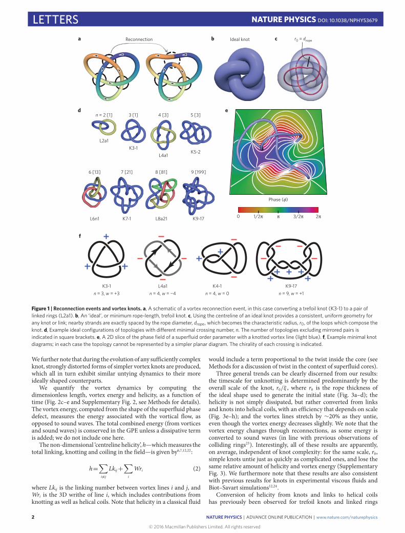
Figure 1 | Reconnection events and vortex knots. a, A schematic of a vortex reconnection event, in this case converting a trefoil knot (K3-1) to a pair oflinked rings (L2a1). b, An ‘ideal’, or minimum rope-length, trefoil knot. c, Using the centreline of an ideal knot provides a consistent, uniform geometry forany knot or link; nearby strands are exactly spaced by the rope diameter, drope, which becomes the characteristic radius, r0, of the loops which compose theknot. d, Example ideal configurations of topologies with di�erent minimal crossing number, n. The number of topologies excluding mirrored pairs isindicated in square brackets. e, A 2D slice of the phase field of a superfluid order parameter with a knotted vortex line (light blue). f, Example minimal knotdiagrams; in each case the topology cannot be represented by a simpler planar diagram. The chirality of each crossing is indicated.

We further note that during the evolution of any sufficiently complexknot, strongly distorted forms of simpler vortex knots are produced,which all in turn exhibit similar untying dynamics to their moreideally shaped counterparts.

We quantify the vortex dynamics by computing thedimensionless length, vortex energy and helicity, as a function oftime (Fig. 2c–e and Supplementary Fig. 2, see Methods for details).The vortex energy, computed from the shape of the superfluid phasedefect, measures the energy associated with the vortical flow, asopposed to sound waves. The total combined energy (from vorticesand sound waves) is conserved in the GPE unless a dissipative termis added; we do not include one here.

The non-dimensional ‘centreline helicity’, h—whichmeasures thetotal linking, knotting and coiling in the field—is given by6,7,12,22:

h=∑i 6=j

Lkij+∑

i

Wri (2)

where Lkij is the linking number between vortex lines i and j, andWri is the 3D writhe of line i, which includes contributions fromknotting as well as helical coils. Note that helicity in a classical fluid

would include a term proportional to the twist inside the core (seeMethods for a discussion of twist in the context of superfluid cores).

Three general trends can be clearly discerned from our results:the timescale for unknotting is determined predominantly by theoverall scale of the knot, r0/ξ , where r0 is the rope thickness ofthe ideal shape used to generate the initial state (Fig. 3a–d); thehelicity is not simply dissipated, but rather converted from linksand knots into helical coils, with an efficiency that depends on scale(Fig. 3e–h); and the vortex lines stretch by ∼20% as they untie,even though the vortex energy decreases slightly. We note that thevortex energy changes through reconnections, as some energy isconverted to sound waves (in line with previous observations ofcolliding rings23). Interestingly, all of these results are apparently,on average, independent of knot complexity: for the same scale, r0,simple knots untie just as quickly as complicated ones, and lose thesame relative amount of helicity and vortex energy (SupplementaryFig. 3). We furthermore note that these results are also consistentwith previous results for knots in experimental viscous fluids andBiot–Savart simulations12,24.

Conversion of helicity from knots and links to helical coilshas previously been observed for trefoil knots and linked rings

2

© 2016 Macmillan Publishers Limited. All rights reserved

NATURE PHYSICS | ADVANCE ONLINE PUBLICATION | www.nature.com/naturephysics

NATURE PHYSICS DOI: 10.1038/NPHYS3679 LETTERS

t′ = 1 t′ = 2 t′ = 3 t′ = 4 t′ = 5

1.4 1.2 1.5

1.0

0.5

0.0

1.1

1.0

0.9

0.8

1.3

1.2

1.1

1.0

0.9

0.5

1.0

Frac

tion

untie

d/un

linke

d

0.00 2 4 6

Rela

tive

leng

th (L

/L0)

[N = 322] [N = 322] [N = 322] [N = 269/322]

8 0 Rela

tive

vort

ex e

nerg

y (E

v/E 0

)

2 4 6 8

K6-2 L4a1 L2a1 Unknot(s)K3-1

=+

a

cb d e

Time (t × /r02)Γ Time (t × /r0

2)Γ0 2 4 6 8 0 2 4 6

h0 ≥ 1

8

Rela

tive

helic

ity (h

/h0)

Time (t × /r02)Γ Time (t × /r0

2)Γ

r0 = 50ξ

300(6r0)

ξ

Figure 2 | Geometric evolution of vortex knots. a, The untying of a randomly distorted 6-crossing knot (K6-2, r0=50ξ) to a collection of unknotted rings.The rescaled time, t′= t×Γ/r02, is shown for each step. The top section shows density iso-surfaces of the local order parameter (red, |ψ |2= 1/2) and thetransparent surfaces (teal or purple) show a constant phase iso-surface. Each volume has been centred on the vortex, which would otherwise have a netvertical motion; only 48% of the simulation volume is shown. b, The fraction of simulations that have untied/unlinked as a function of time, computed forthe 322 simulations of ideal knots with r0=50ξ . The median unknotting time is indicated in red. c–e, 2D histograms of relative length, vortex energy andhelicity as a function of time for all prime topologies with n≤9. The dashed lines indicate average values. The helicity histogram (e) includes only the269/322 topologies with h0≥ 1. See Supplementary Fig. 2 for similar histograms for each group of simulations.

a

Coun

ts

Coun

ts

50 n = 9n = 8n ≤ 740

30

20

10

10

Unt

ied

helic

ity (h

untie

) 8

6

4

2

0

0 2 4

huntie ∼ 0.61h0 huntie ∼ 0.68h0 huntie ∼ 0.74h0 huntie ∼ 0.66h0

6Initial helicity (h0)

8 10 12 0 2 4 6Initial helicity (h0)

8 10 12 0 2 4 6Initial helicity (h0)

8 10 12 0 2 4 6Initial helicity (h0)

8 10 12

10

Unt

ied

helic

ity (h

untie

) 8

6

4

2

0

10

Unt

ied

helic

ity (h

untie

) 8

6

4

2

0

10

Unt

ied

helic

ity (h

untie

) 8

6

4

2

0

0

50

40

30

20

10

0

Coun

ts

Coun

ts

50 706050403020100

40

30

20

10

00 2 4 6 8 10 12 14

b c d

e f g h

Untying time (tuntie × /r02)Γ Untying time (tuntie × /r0

2)Γ Untying time (tuntie × /r02)Γ Untying time (tuntie × /r0

2)Γ0 2 4 6 8 10 12 14 0 2 4 6 8 10 12 14 0 2 4 6 8 10 12 14

= 0.25r0σr0 = 15ξ

r0 = 50ξr0 = 25ξr0 = 15ξ

Figure 3 | Statistics of vortex knot untying. Histograms of the rescaled untying time (a–d) and the untied versus initial helicity (e–h) for four di�erentgroups of simulations: a–c,e–g, All 322 ideal knots with n≤9 at a scale of r0={15,25,50}ξ . d,h, Four randomly distorted versions of each n≤8 ideal knotwith r0= 15ξ and σ =0.25r0 (492 simulations total). a–d, The distribution of untying times is well described by a log-normal distribution (dashed red line):P(t′)∝(1/t′)exp[−(( ln t′−µ)2/(2σ 2))], where the average unknotting time is 〈t′〉≈expµ={4.0,3.9,3.5,3.7} and the spread is σ ={0.37,0.41,0.44,0.47}for a–d respectively. e–h, The final helicity is approximately proportional to the initial helicity (red line). The degree to which helicity is preserved dependson overall scale, but is apparently only slightly a�ected by randomly distorting the knots. (This slight di�erence might be explained by the knots beinge�ectively larger from the distortion.)

in classical fluids12, and can be explained through a geometricmechanism. After each reconnection event, helices with a rangeof length scales are produced on the reconnected vortices. If oneassumes a perfectly antiparallel reconnection without any spatialcutoff, this process is expected to exactly conserve helicity12,25.However, in the GPE, helical distortions on the scale of the

healing length are radiated away as sound waves (SupplementaryMovie 4). As a result, we observe an average helicity losswith an approximate 1h/h0∝ (r0/ξ)−0.5 trend. Remarkably, theseresults suggest that as the scale becomes very large, r0 � ξ ,helicity conservation should be recovered even though knotsstill untie.

NATURE PHYSICS | ADVANCE ONLINE PUBLICATION | www.nature.com/naturephysics

© 2016 Macmillan Publishers Limited. All rights reserved

3

LETTERS NATURE PHYSICS DOI: 10.1038/NPHYS3679

−2n, +2w −1n

−1w

−1n

−1w

−1n

−1w

−1n

−1w

−1n

−1w

1 reconnection + untwisting(2 × Reidemeister type I)

Relaxation of antiparallel pair

3 separate reconnections

Relaxation of parallel pair

n = 4w = 4

n = 6w = 2

n = 3w = 3

n = 2w = 2

−3n

−3w

b c

a

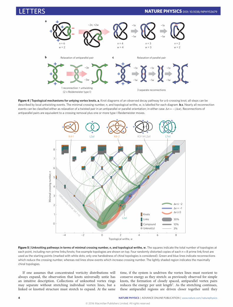
Figure 4 | Topological mechanisms for untying vortex knots. a, Knot diagrams of an observed decay pathway for a 6-crossing knot; all steps can bedescribed by local untwisting events. The minimal crossing number, n, and topological writhe, w, is labelled for each diagram. b,c, Nearly all reconnectionevents can be classified either as relaxation of a twisted pair in an antiparallel or parallel orientation; in either case1n=−|1w|. Reconnections ofantiparallel pairs are equivalent to a crossing removal plus one or more type-I Reidemeister moves.

L2a1

L2a1

8

Min

imal

cro

ssin

g nu

mbe

r, n

7

6

5

4

3

2

1

0

−4 −2 0 2

Knots

Links

10%

30%

Δn ≤ −2Δn = −1Δn ≥ 0

3%CompoundUnknot(s)

Topological writhe, w

(Maximally chiral: |w| = n)

4 6 8

L7n1K4-1 K3-1 # L2a1K8-2

Figure 5 | Unknotting pathways in terms of minimal crossing number, n, and topological writhe, w. The squares indicate the total number of topologies ateach point, including non-prime links/knots; five example topologies are shown on top. Four randomly distorted copies of each n=8 prime link/knot areused as the starting points (marked with white dots; only one handedness of chiral topologies is considered). Green and blue lines indicate reconnectionswhich reduce the crossing number, whereas red lines show events which increase crossing number. The lightly shaded region indicates the maximallychiral topologies.

If one assumes that concentrated vorticity distributions willalways expand, the observation that knots universally untie hasan intuitive description. Collections of unknotted vortex ringsmay separate without stretching individual vortex lines, but alinked or knotted structure must stretch to expand. At the same

time, if the system is undriven the vortex lines must reorient toconserve energy as they stretch: as previously observed for simpleknots, the formation of closely spaced, antiparallel vortex pairsreduces the energy per unit length3. As the stretching continues,these antiparallel regions are driven closer together until they

4

© 2016 Macmillan Publishers Limited. All rights reserved

NATURE PHYSICS | ADVANCE ONLINE PUBLICATION | www.nature.com/naturephysics

NATURE PHYSICS DOI: 10.1038/NPHYS3679 LETTERSultimately reconnect; this process continues until the knots arecompletely untied. We note that, in most cases, the stretching stopsabruptly after the knots finish untying (Supplementary Fig. 1), inagreement with this interpretation. Interestingly, such a picturealso naturally produces the antiparallel reconnection geometry thatfavours helicity conservation.

Although the above results demonstrate the overwhelmingtendency for vortex knots to untie, they do not elucidate the specifictopological pathways which produce this untangling. To measurethese unknotting sequences, we identify the topology, Ti, of thevortices after each reconnection by computing their HOMFLY-PT polynomials26,27. Owing to the high degree of symmetry ofideal knots, reconnections are often nearly coincident in time,preventing identification of the intermediate topology. To avoid thiscomplication, we consider only the decays of the randomly distortedknots, which break this symmetry.

The first question we examine is whether the knot is simplifyingat each step. We quantify the knot complexity by means of thecrossing number, n, of each knot in a minimal two-dimensional(2D) diagram (Fig. 1f), which is a topological invariant of theknot. Supplementary Table 2 shows the statistics of the jumps inthe crossing number through all reconnections, revealing knots areabout an order of magnitude more likely to ‘untie’ (1n< 0) than‘retie’ (1n>0) at each individual reconnection. On average, morethan one crossing is removed with each reconnection, underscoringthe fact that physical reconnections of vortices in 3D are notequivalent to removing (or adding) a single crossing from a 2Dminimal knot diagram. Nonetheless, the minimal diagrams reveala clear trend towards topological simplification.

If each reconnection does not correspond to ‘removing’ asingle crossing from a 2D knot diagram, is it still possible toproduce an intuitive description of these events in terms of suchdiagrams? This question can be answered by considering the 2Dtopological writhe, w(Ti), which is obtained by summing thehandedness (±1) of each crossing in a minimal knot diagram(obtained from ref. 28). Remarkably, we find that the vast majority(96.1%) of reconnection events only add/remove crossings of thesame sign from 2D diagrams, that is, |1n| = |1w| (includingevents with remove a single crossing). As shown in Fig. 4b,c,reconnections which satisfy this condition are equivalent to therelaxation of a parallel or antiparallel pair in a 2D diagram. Forthe perspective of minimal diagrams, the removal of multiplecrossings occurs by a single reconnection in an antiparallel pair,followed by the untwisting of a topologically trivial loop by type-IReidemeister moves29,30 (Fig. 4b). Reconnections followed by morecomplicated simplifications are possible (for example, incorporatingtype-II Reidemeister moves); however, such events are observed tobe rare.

Figure 5 and SupplementaryMovie 5 show the topological writheand crossing number of every knot with n≤ 8, including non-prime topologies, connected by lines indicating the frequency ofthe observed unknotting pathways. (This is similar to diagramswhich have previously been constructed for mathematical knotsimplification of a different type31.) In addition to illustratingthe above results, this diagram reveals the importance of the‘maximally chiral’ topologies, for which |w| = n. The topologicalwrithe for any particular knot or link is bounded by the numberof crossings; maximally chiral knots and links saturate this bound,which corresponds to every crossing having the same sign.

Despite the fact that only around a third of all n≤8 topologiesare maximally chiral, 82.6% of jumps end in such a state. Thedominance of this pathway has a simple interpretation: if we assumeall reconnections satisfy |1n| ≥ |1w|, corresponding to a slopeof |1n/1w| ≥ 1 in Fig. 5, once the vortex knot decays into amaximally chiral topology it can leave such a state only by increasingits crossing number. (Although the observation that |1n| ≥ |1w|

seems self-evident when considering minimal crossing diagrams,we are not aware of a proof of this relationship. Nonetheless, wenever observe reconnections which violate it.) Indeed, owing tothe ‘gap’ between maximally and non-maximally chiral states, thecrossing number must increase by 1n≥+2 to leave the maximallychiral branch. Moreover, even in the event that the crossing numberdoes increase by this amount, we observe that it still typically stayson the maximally chiral branch. Thus, statistically, most knots arefunnelled into a maximally chiral pathway during their untying,after which they decay only along this pathway.

Our observation of a preferred maximally chiral pathway isa generalization of a previously known result for site-specificrecombination of DNA knots: any p= 2 torus knot/link (whichare all maximally chiral) may convert into another p= 2 torusknot by means of reconnections only if the crossing number isdecreasing2. Our results indicate that this torus knot pathway isone example of a more general phenomena. Intuitively, this suggestsuntangling knots tend to end up in states which are twisted in onlyone chiral direction.

Taken as a whole, we find that the topological behaviour ofsuperfluid vortex knots and links can be understood through simpleprinciples. All vortex knots untie, and they tend to do so efficiently:monotonically decreasing their crossing number until they area collection of unknotted vortices. This suggests that non-trivialvortex topology in superfluids—or any fluidwith similar topologicaldynamics—should arise only from external driving. Even in thepresence of driving, the observed decay pathways indicate thatvortices would probably settle into a maximally chiral topology; itwould be of great interest to probe for such states in superfluid orclassical turbulence.

The evolution and untying dynamics of the superfluid knotswe observe is strongly reminiscent of those in classical fluidsand DNA recombination2,3,12. These similarities persist despitefundamental differences between these systems, especially withregards to the small-scale details of the reconnection processesthat drive topology changes. This suggests that they might applyeven more generally, forming a universal set of mechanisms forunderstanding the evolution of knots in a variety of dissipativephysical systems.

MethodsMethods and any associated references are available in the onlineversion of the paper.

Received 23 September 2015; accepted 25 January 2016;published online 7 March 2016

References1. Raymer, D. M. & Smith, D. E. Spontaneous knotting of an agitated string. Proc.

Natl Acad. Sci. USA 104, 16432–16437 (2007).2. Shimokawa, K., Ishihara, K., Grainge, I., Sherratt, D. J. & Vazquez, M.

FtsK-dependent XerCD-dif recombination unlinks replication catenanes in astepwise manner. Proc. Natl Acad. Sci. USA 110, 20906–20911 (2013).

3. Kleckner, D. & Irvine, W. T. M. Creation and dynamics of knotted vortices.Nature Phys. 9, 253–258 (2013).

4. Cirtain, J. W. et al . Energy release in the solar corona from spatially resolvedmagnetic braids. Nature 493, 501–503 (2013).

5. Thomson, W. On vortex atoms. Philos. Mag. XXXIV, 94–105 (1867).6. Moffatt, H. K. Degree of knottedness of tangled vortex lines. J. Fluid Mech. 35,

117–129 (1969).7. Berger, M. A. Introduction to magnetic helicity. Plasma Phys. Control. Fusion

41, B167–B175 (1999).8. Proment, D., Onorato, M. & Barenghi, C. Vortex knots in a Bose–Einstein

condensate. Phys. Rev. E 85, 1–8 (2012).9. Wasserman, S. A. & Cozzarelli, N. R. Biochemical topology: applications to

DNA recombination and replication. Science 232, 951–960 (1986).10. Tkalec, U. et al . Reconfigurable knots and links in chiral nematic colloids.

Science 333, 62–65 (2011).

NATURE PHYSICS | ADVANCE ONLINE PUBLICATION | www.nature.com/naturephysics

© 2016 Macmillan Publishers Limited. All rights reserved

5

LETTERS NATURE PHYSICS DOI: 10.1038/NPHYS3679

11. Bewley, G. P., Paoletti, M. S., Sreenivasan, K. R. & Lathrop, D. P.Characterization of reconnecting vortices in superfluid helium. Proc. NatlAcad. Sci. USA 105, 13707–13710 (2008).

12. Scheeler, M. W., Kleckner, D., Proment, D., Kindlmann, G. L. & Irvine, W. T. M.Helicity conservation by flow across scales in reconnecting vortex links andknots. Proc. Natl Acad. Sci. USA 111, 15350–15355 (2014).

13. Sumners, D. Lifting the curtain: using topology to probe the hidden action ofenzymes. Not. Am. Math. Soc. 528–537 (1995).

14. Woltjer, L. A theorem on force-free magnetic fields. Proc. Natl Acad. Sci. USA44, 489–491 (1958).

15. Moffatt, H. & Ricca, R. Helicity and the Calugareanu invariant. Proc. R. Soc.Lond. A 439, 411–429 (1992).

16. Barenghi, C. F. Knots and unknots in superfluid turbulence.Milan J. Math. 75,177–196 (2007).

17. Dennis, M. R., King, R. P., Jack, B., O’holleran, K. & Padgett, M. Isolated opticalvortex knots. Nature Phys. 6, 118–121 (2010).

18. Martinez, A. et al . Mutually tangled colloidal knots and induced defect loops innematic fields. Nature Mater. 13, 258–263 (2014).

19. Pitaevskii, L. P. & Stringari, S. Bose–Einstein Condensation (Clarendon, 2003).20. Pieranski, P. in Ideal Knots (eds Stasiak, A., Katritch, V. & Kauffman, L. H.)

(World Scientific, 1998).21. Katritch, V. et al . Geometry and physics of knots. Nature 384, 142–145 (1996).22. Akhmet’ev, P. & Ruzmaikin, A. in Topological Aspects of the Dynamics of Fluids

and Plasmas Vol. 218 (eds Moffatt, H. K., Zaslavsky, G. M., Comte, P. & Tabor,M.) 249–264 (NATO ASI Series, Springer, 1992).

23. Leadbeater, M., Winiecki, T., Samuels, D. C., Barenghi, C. F. & Adams, C. S.Sound emission due to superfluid vortex reconnections. Phys. Rev. Lett. 86,1410–1413 (2001).

24. Ricca, R. L., Samuels, D. & Barenghi, C. Evolution of vortex knots. J. FluidMech. 391, 29–44 (1999).

25. Laing, C. E., Ricca, R. L. & Sumners, D. W. L. Conservation of writhe helicityunder anti-parallel reconnection. Sci. Rep. 5, 9224 (2015).

26. Freyd, P. et al . A new polynomial invariant of knots and links. Bull. Am. Math.Soc. 12, 239–246 (1985).

27. Przytycki, J. H. & Traczyk, P. Conway algebras and skein equivalence of links.Proc. Am. Math. Soc. 100, 744–748 (1987).

28. Cha, J. C. & Livingston, C. Knot Info: Tables of Knot Invariants (February 2015);http://www.indiana.edu/∼knotinfo

29. Reidemeister, K. Abhandlungen aus dem Mathematischen Seminar derUniversität Hamburg Vol. 5, 24–32 (Springer, 1927).

30. Alexander, J. W. & Briggs, G. B. On types of knotted curves. Ann. Math. 28,562–586 (1926).

31. Flammini, A. & Stasiak, A. Natural classification of knots. Proc. R. Soc. Lond. A463, 569–582 (2007).

AcknowledgementsThe authors acknowledge M. Scheeler and D. Proment for useful discussions. This workwas supported by the National Science Foundation (NSF) Faculty Early CareerDevelopment (CAREER) Program (DMR-1351506), and completed in part withresources provided by the University of Chicago Research Computing Center and theNVIDIA Corporation. W.T.M.I. further acknowledges support from the A.P. SloanFoundation through a Sloan fellowship, and the Packard Foundation through a Packardfellowship.

Author contributionsD.K. and W.T.M.I. designed and developed the study. D.K. performed simulations andknot identification. D.K., L.H.K. and W.T.M.I. analysed data. D.K. and W.T.M.I. wrotethe manuscript.

Additional informationSupplementary information is available in the online version of the paper. Reprints andpermissions information is available online at www.nature.com/reprints.Correspondence and requests for materials should be addressed to D.K. or W.T.M.I.

Competing financial interestsThe authors declare no competing financial interests.

6

© 2016 Macmillan Publishers Limited. All rights reserved

NATURE PHYSICS | ADVANCE ONLINE PUBLICATION | www.nature.com/naturephysics

NATURE PHYSICS DOI: 10.1038/NPHYS3679 LETTERSMethodsSimulation details. The time evolution of the superfluid order parameter wascomputed by numerically integrating the Gross–Pitaevskii equation using asplit-step spectral method along the lines of refs 8,12. For simulations with meanradius r0/ξ={15,25}, we use a grid size of1x=0.5ξ , a simulation time step of1t=0.02, and save the traced vortex paths at an interval of1T=1. Forsimulations with r0=50ξ , we compute a coarser simulation with1x=1ξ ,1t=0.1and1T=4. The radial distance from the vortices at which the order parameter,|ψ |, recovers to half its far-field value (often referred to as the ‘core size’) isdetermined by the healing length and is approximately R∼2ξ . A small number ofsimulations of the same sized knot at different resolutions (1x/ξ={0.25,0.5,1})was used to confirm that the coarser simulations do not significantly affect thecomputed length and helicity of the vortex as it unties (the noise in these computedquantities does increase, but we do not observe systematic differences). The totalsize of the periodic simulation box was L/ξ={128,192,384} for r0/ξ={15,25,50},respectively. Occasionally, small vortex rings ejected from the untying vorticesinteract with their periodic partners by traversing the boundary; in general thishappens only after the vortices have untied. To ensure that the size of the box doesnot affect the behaviour of the knot, we have simulated the same knot in severaldifferently sized periodic volumes; we find that the behaviour of the knot isvirtually identical so long as it is spaced more than a few r0 from its periodicpartner (in practice, the most complex knots have a maximum extent of onlyaround half the length of edge of the simulation box).

We note that we employ a version of the GPE without dissipation, and so thetotal energy is conserved. Numerically, there is some small loss (always less than 1%and typically less than 0.2%), which is not significant for any of our results. We alsoinclude a chemical potential of µ=−1 (in dimensionless units) in our definition ofthe GPE; this is added to remove an overall phase rotation. Removing thisadditional term would produce mathematically identical results, as the overallphase is not physically significant.

Initial state construction. The phase fields for the initial states were generated bybrute force integration of a Biot–Savart-generated flow field, uBS, which is related tothe phase gradient through the relationship:

∇φ(x)=uBS(x) (3)

This method is described in more detail in ref. 12. An example an initial phase fieldis shown in Fig. 1e and Supplementary Movie 1.

The initial density field, ρ=|ψ |2, was calculated using an approximate formobtained for an infinite, straight vortex line32:

ρ(r)=1132 r

2+

11384 r

4

1+ 13 r 2+

11384 r 4

(4)

where r was taken to be the distance to the closest vortex line.To ensure consistency between different topologies, we choose the ‘ideal’ form

of each knot, equivalent to the shape of the shortest knot tied in a finite thicknessrope (Fig. 1b–d; ref. 20). These canonical shapes are known to capture aspects ofthe knot type as well as approximating the average properties of random knots21,making them a useful reference geometry for each topology. The shapes of idealknots for different topologies were obtained from an online source(http://katlas.math.toronto.edu/wiki/Ideal_knots), and were initially generated bymeans of the SONOmethod20.

To create randomly distorted knots, we compute a random normally distributedvector, δ, for each point in a polygonal representation of the vortex knot inquestion. We then smooth this vector with a Gaussian of width σ =0.5r0 (measuredalong the path of original vortex line), remove the component tangential to theoriginal knot path, and rescale the displacement vector so that 〈|δ|2〉=(0.25r0)2.This displacement is added to the original coordinates to obtain the distorted knot.Examples of randomly distorted knots are shown in Fig. 2a and the inset of Fig. 3d.For the data shown in the paper, four randomly perturbed copies of each n≤8knot/link (4×123 configurations) were considered at a scale of r0=15ξ . A smallnumber of randomly distorted knots at larger scales were considered, producingqualitatively similar effects to the scaling of undistorted ideal knots.

Quantification of vortex behaviour. For each saved time step, a polygonalrepresentation of the vortex shape is obtained by tracing the phase defects in thesuperfluid order parameter with a resolution set by the simulation grid (typicallyresulting in&103 points total). In addition, a phase normal, φ̂, is computed foreach point on the vortex by finding the direction of zero phase which isperpendicular to the vortex path. All subsequent properties (vortex energy, helicity,and length) are computed from this path.

To determine the moment which a knot finishes untying, we find the momentat which its HOMFLY-PT polynomial is equivalent to unknots (see ‘Identificationof Vortex Topology’ below). A histogram of the unknotting times, Fig. 3a–d, isconsistent with a log-normal distribution. We find that once the time is

appropriately rescaled, the mean unknotting times for each simulation group are inthe range 〈tunknot〉≈(3.5−4.0) r 02/Γ (r0 is the diameter of the ‘rope’ in which theideal knot is tied).

As stated in the main text, we compute the centreline helicity in thedimensionless form:

h=∑i 6=j

Lkij+∑

i

Wri (5)

Although this can be computed directly from the polygonal paths, this methodrequires special considerations for dealing with linking across periodic boundaries.Alternatively, we may note that a surface of constant phase defines a ‘Seifertframing’ for each knot/link obeying h+

∑iTwφ,i=0 (ref. 22), where Twφ,i is the

twist of the phase normal about the vortex path:

Twφ,i=

∮Ci

d`· φ̂×∂sφ̂ (6)

where Ci refers to closed vortex path i, ∂s is a path-length derivative and φ̂ is a unitvector that is lies along a surface of equal phase and is perpendicular to the tangentvector of the vortex line at that point. As the total twist can be easily numericallyintegrated from the vortex path and phase normal, it provides an efficient methodfor computing centreline helicity. We have numerically confirmed that this methodprovides results equal to direct computation of linking and writhe, up to numericalprecision.

The energy associated with the vortices in the superfluid (as opposed to soundwaves), Ev, is computed from the ‘path inductance’3, Eij, of the vortex centrelines:

Ev∼=ρΓ 2

2∑

ij

Eij (7)

Eij=14π

|ri−rj |> ξ2∮

Ci

∮Cj

dri ·drj∣∣r−rj∣∣ +δij 2−α2πLi (8)

where Li is the total length of vortex loop i.Here, α∼=1.615 is a dimensionless correction factor chosen to obtain the

correct value for the energy of a vortex ring in the GPE (ref. 33). To account for theperiodic nature of the simulations, the cross inductance is included for a 3×3×3periodic array of vortex paths (including more periodic copies improves theaccuracy of the calculation, but the difference is typically only a small fraction of aper cent). Note that the total energy in the superfluid is conserved, so a reductionin vortex energy corresponds to an increase in the energy in sound waves. The vastmajority of energy changes in the vortices are seen to occur during or immediatelyafter reconnection events; otherwise the computed energy is nearly constant.

Identification of vortex topology. To identify the topology of the superfluidvortices at each time step, the polygonal vortex representation is first reduced to theminimum possible number of points possible without changing the topology(unknots are also removed at this stage, if they are not threaded by any other vortexlines). Once the vortices are reduced, they are projected into an arbitrary 2D planeand the projected crossings and their handedness are identified; the HOMFLY-PTpolynomial is created directly from this crossing list. This polynomial is comparedagainst an internally generated database of HOMFLY-PT polynomials for alltopologies (including chiral pairs, oriented links, and disjoint and compoundknots/links) with a minimal crossing number of n≤10. As mentioned in the maintext, we label topologies following the format used by the ‘Knot Atlas’,http://katlas.org, for example, a ‘stevedore’s knot’ is K6-1, with the ‘K’ indicating itis a knot (versus a link, ‘L’), n=6 is the minimal crossing number (Fig. 1f), and theremainder indicates an arbitrary ordering.

The database of HOMFLY-PT polynomials for prime topologies was generatedstarting from the crossing diagrams obtained from ref. 28. The equivalenceof oriented links was determined by assuming all orientational permutations withidentical HOMFLY-PT polynomials are topologically equivalent. The HOMFLY-PTpolynomial of disjoint and compound topologies was computed algebraicallyfrom the HOMFLY-PT polynomials of their components, and added to the list.We do not treat configurations with extra unknots to be distinct topologies, and donot distinguish between disjoint and compound topologies. (We note that disjointknots are rarely observed in the decay pathways, and are furthermore difficultto distinguish from compound knots by means of HOMFLY-PT polynomials ifunknots are also present.) There exist several knots/links with identical HOMFLY-PT polynomials for n≥9, but we do not encounter any of these in the observedpathways for knots starting with n≤8, which were used to compute decay pathways.

References32. Berloff, N. G. Padé approximations of solitary wave solutions of the

Gross–Pitaevskii equation. J. Phys. A 37, 1617–1632 (2004).33. Donnelly, R. J. Vortex rings in classical and quantum systems. Fluid Dyn. Res.

41, 051401 1–31 (2009).

NATURE PHYSICS | www.nature.com/naturephysics

© 2016 Macmillan Publishers Limited. All rights reserved