How the Bundesbank really conducted monetarypolicy: An analysis based on real-time data

Christina Gerberding(Deutsche Bundesbank)

Andreas Worms(Deutsche Bundesbank)

Franz Seitz(Fachhochschule Amberg-Weiden)

Discussion PaperSeries 1: Studies of the Economic Research CentreNo 25/2004

Discussion Papers represent the authors’ personal opinions and do not necessarily reflect the views of theDeutsche Bundesbank or its staff.

Editorial Board: Heinz HerrmannThilo LiebigKarl-Heinz Tödter

Deutsche Bundesbank, Wilhelm-Epstein-Strasse 14, 60431 Frankfurt am Main,Postfach 10 06 02, 60006 Frankfurt am Main

Tel +49 69 9566-1Telex within Germany 41227, telex from abroad 414431, fax +49 69 5601071

Please address all orders in writing to: Deutsche Bundesbank,Press and Public Relations Division, at the above address or via fax No +49 69 9566-3077

Reproduction permitted only if source is stated.

ISBN 3–86558–014–9

Abstract:

Papers estimating the reaction function of the Bundesbank generally find that itsmonetary policy from the 1970s to 1998 can well be captured by a standard Taylor ruleaccording to which the central bank responds to the output gap and to deviations ofinflation from target, but not to monetary growth. This result is at odds with theBundesbank´s claim that it followed a strategy of monetary targeting. This paperanalyses whether this apparent contradiction is due to (a) the use of ex post data whichdo not necessarily match policy makers’ real-time information sets and (b) the omissionof important explanatory variables. Accordingly, we compile a real-time data set forGermany including the Bundesbank’s own estimates of potential output and use it to re-estimate the Bundesbank’s reaction function. We find that the use of real-time dataconsiderably changes the results. Moreover, when adding the change in the output gapas well as deviations of money growth from target to the set of explanatory variables,we find that both variables are highly significant. This suggests that the Bundesbanktook its monetary targets seriously, but also responded to deviations of expectedinflation and output growth from target.

Keywords: E43, E52, E58

JEL-Classification: Monetary policy, Taylor rule, real-time data, Bundesbank

Non-Technical Summary

The inflation record of the Bundesbank in the 1970s and early 1980s was better than

that of many other central banks. A distinctive feature of the Bundesbank´s monetary

policy since 1975 was that it announced targets for monetary growth and - according to

its own descriptions - based monetary policy decisions on deviations of actual money

growth from these targets. However, contrary to that description, recent empirical

studies generally find that monetary aggregates did not play a significant role for the

Bundesbank´s interest rate decisions. We find that this “contradiction” can be explained

by two deficiencies of the respective empirical analyses. First, the use of ex-post revised

data ignores that the data and estimates relevant for monetary policy decisions

underwent major revisions in the course of time and, second, these studies restrict the

set of explanatory variables only to those contained in the Taylor rule plus a variable

that serves to capture monetary targeting.

To test the implications of the data revisions, we have compiled a real-time data set

which includes real and nominal output, the Bundesbank’s own estimates of potential

output, the inflation rate (measured by consumer prices and the GDP deflator) and the

growth rate of the official monetary target variable. While we are able to reproduce the

result of the previous literature on the basis of ex-post data - i.e. we find that the

Bundesbank´s policy can be described fairly well by a standard Taylor rule - this result

does not hold if we use real-time data. More specifically, we find that the Bundesbank

based its monetary policy decisions on the (real-time) expected inflation gap, but not on

its (real-time) estimate of the output gap.

Instead, the Bundesbank’s own regular reports on the economic situation in Germany

during the period in question (1975-1998) point into the direction that concern about

economic activity and the economic outlook focused on the growth in output (relative to

the growth in potential) rather than on the level of output (relative to the level of

potential). Therefore, we add the change in the output gap as well as deviations of

money growth from target to the set of explanatory variables. We find that both

variables are highly significant, whereas the level of the real-time output gap still drops

out. This suggests that the Bundesbank took its monetary targets seriously, but also

responded to deviations of expected inflation and output growth from the respective

targets.

Nichttechnische Zusammenfassung

Das Ergebnis der Bundesbankpolitik hinsichtlich der Preisstabilität war in den 70er und

frühen 80er Jahren besser als das vieler anderer Zentralbanken. Ein besonderes

Merkmal der Bundesbankpolitik war dabei, dass sie seit 1975 ein jährliches

Geldmengenziel verkündete und - ihren eigenen Aussagen nach - ihre geldpolitischen

Entscheidungen auf Abweichungen des tatsächlichen Geldmengenwachstums von

diesem Ziel basierte. Im Gegensatz hierzu haben neuere empirische Studien jedoch

gefunden, dass die Geldmenge keine signifikante Rolle bei den Zinsentscheidungen der

Bundesbank spielte. Wir finden, dass dieser “Widerspruch” durch zwei Schwachstellen

dieser empirischen Arbeiten erklärt werden kann. Zum einen vernachlässigt die

Verwendung ex-post revidierter Daten, dass Daten und Schätzungen, die den

geldpolitischen Entscheidungen in Echtzeit zugrunde lagen, im Laufe der Zeit

gravierend revidiert wurden. Zum anderen berücksichtigen diese empirischen Studien

lediglich jene Variablen, die sich in der Taylor-Regel befinden, zuzüglich einer

Geldmengengröße und keine weiteren Variablen.

Um die Implikationen der Datenrevisionen abschätzen zu können, haben wir einen

Echtzeitdatensatz konstruiert. Er enthält die reale Produktion, das nominale

Volkseinkommen, die Bundesbank-eigenen Schätzungen des Produktionspotenzials, die

Inflationsrate (gemessen auf Basis des Konsumentenpreisindex und des BIP-Deflators)

und die Wachstumsrate der offiziellen Geldmengen-Zielgröße. Während wir die

Ergebnisse der früheren empirischen Arbeiten mit ex-post Daten reproduzieren können,

d. h. wir finden auf Basis revidierter Daten, dass die Bundesbankpolitik gut durch eine

gewöhnliche Taylor-Regel beschrieben werden kann, hat dieses Resultat auf Basis von

Echtzeitdaten keinen Bestand mehr. Insbesondere ergibt sich, dass die Bundesbank ihre

geldpolitischen Entscheidungen auf die erwarteten (Echtzeit-)Inflationslücken stützte,

nicht aber auf ihre (Echtzeit-)Schätzung der Produktionslücke.

Statt dessen deuten die eigenen regelmäßigen Berichte der Bundesbank aus der

fraglichen Zeit (1975-1998) an, dass ihre Konjunkturanalyse und -ausblick sich auf das

Produktionswachstum (relativ zum Potenzialwachstum) und weniger auf das

Produktionsniveau (relativ zum Potenzialniveau) bezog. Daher fügen wir die Änderung

der Produktionslücke gemeinsam mit der Abweichung der Geldmengenwachstumsrate

vom Ziel als zusätzliche erklärende Variablen in die Schätzung ein. Wir finden, dass

beide Variablen hochsignifikant sind, während das Niveau der Echtzeit-

Produktionslücke weiterhin nicht signifikant ist. Dies bedeutet, dass die Bundesbank

ihre Geldmengenziele durchaus ernst genommen hatte, dass sie aber auch auf die

Abweichungen der erwarteten Inflationsrate und des Produktionswachstums von den

jeweiligen Zielwerten reagierte.

Contents

1 Introduction 1

2 Specification of the Central Bank’s Reaction Function 4

3 Reconstruction of the Bundesbank’s real-time data set 6

4 The econometric approach 14

4.1 Derivation of an estimable equation 14

4.2 Basic specification with ex post data 17

4.3 Basic specification with real-time data 18

4.4 Extensions of the basic specification 19

5 Interpretation 23

6 Outlook 26

References 27

Lists of Tables and Figures

Table 1 Structure of the real-time data set for GNP/GDP

Table 2 Structure of the real-time data set for potential output

Table 3 Structure of the real-time data set for the output gap

Table 4 Summary statistics on revisions of real-time output gaps

Table 5 Structure of the real-time data set for CPI inflation

Table 6 Medium-term price assumption 1975 – 1998

Table 7 Structure of the real-time data set for the respective

monetary target variable

Table 8 Parameter estimates of the baseline reaction function

with ex post revised data

Table 9 Parameter estimates of the baseline reaction function

with real-time data

Table 10 Monetary targets and their implementation

Table 11 Parameter estimates of the reaction function with

additional variables

Table 12 Robustness of results for different horizons of the money

growth variable (with n=5)

Figure 1 Initial and ex post data on growth of real GNP/GDP

Figure 2 Initial and ex post data on change of GNP/GDP deflator

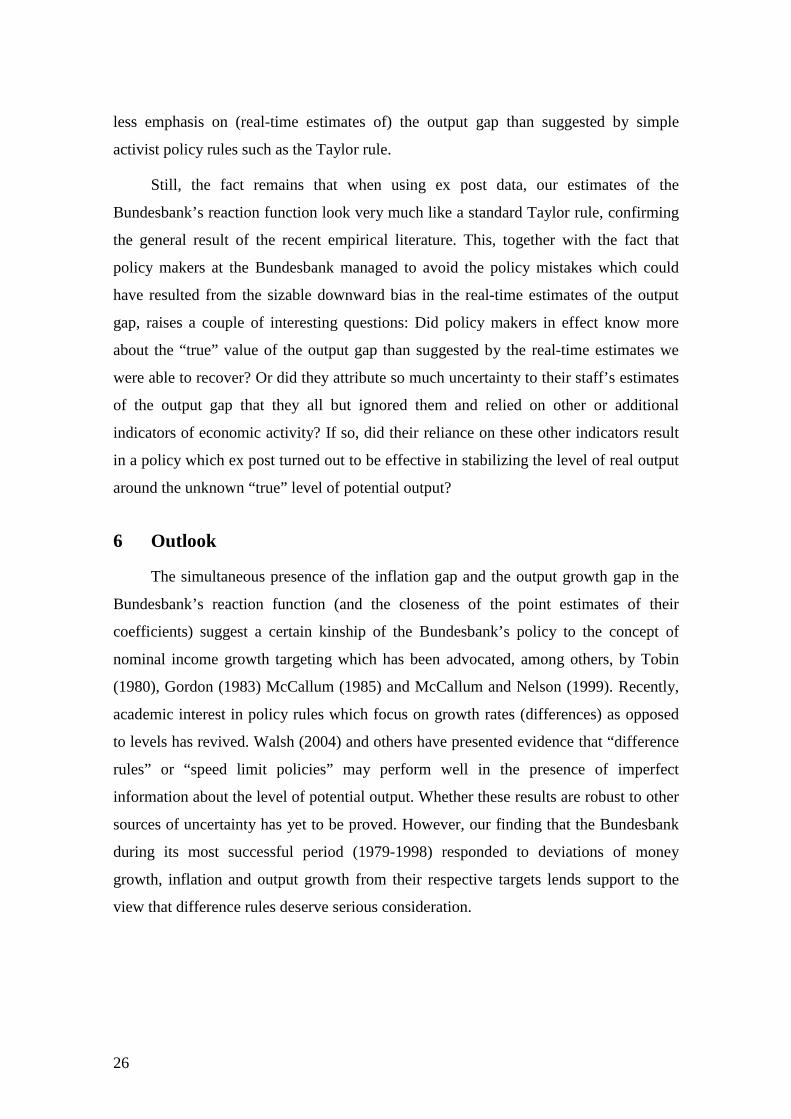
Figure 3 Initial and ex post estimates of the output gap

Figure 4 Initial and ex post estimates of the change in the output

gap

Figure 5 Measurement errors of output gap and change in the gap

Figure 6 Initial and ex post data on CPI inflation

Figure 7 Real-time inflation gaps - CPI versus output deflator

Figure 8 Initial and ex post data on the respective monetary target

variables

Figure 9 Overnight and three month interest rates in Germany

(end-of-quarter values)

Figure 10 The time pattern for i and π

1

How the Bundesbank really conducted monetary policy:An analysis based on real-time data*

1 Introduction

The question of how the Bundesbank conducted monetary policy is of interest not

just from a historical perspective. Given that the Bundesbank is usually seen as a

comparatively successful central bank it may be useful to better understand its monetary

policy in order to draw conclusions for current monetary policy. For example, there is

an ongoing discussion about the interpretation of the US-Fed’s monetary policy in the

1970s. While some commentators argue that the Fed was responsible for the “Great

Inflation” of the 1970s because its monetary policy was too expansionary compared

with a Taylor rule (according to which the short-term real interest rate should be raised

if inflation increases above the target level and/or if real output rises above trend),

others stress that such an interpretation relies on the advantage of hindsight: Today, we

know that the Fed´s real-time assessment of the US business cycle was too pessimistic.

Taking this real-time problem into account, the Fed´s monetary policy could be justified

even from a Taylor-rule perspective. Or, to put it differently, the Fed´s policy would not

have been significantly different had it in fact followed a Taylor rule.

The inflation record of the Bundesbank in the 1970s and early 1980s was better

than that of the Fed and many other central banks and one could ask whether the

Bundesbank was able to avoid some of the “mistakes” made by others and – if so – why

this was the case. One obvious distinctive feature of the Bundesbank´s monetary policy

since 1975 was that it announced annual targets for monetary growth and – according to

its own descriptions – based monetary policy decisions on deviations of actual money

growth from these targets. However, recent empirical studies that analyse the

Bundesbank´s monetary policy generally find that monetary aggregates did not play a

* We thank J. Breitung, J. Doepke, C. Evans, D. Gerdesmeier, O. Issing, R. König, A. Orphanides, J.H.

Rogers, P. Schmid, J.-E. Sturm, J. v. Hagen and seminar participants of the Bundesbank and theBundesbank Conference on Real-time data and Monetary Policy in Eltville for helpful comments andinformations. We also appreciate the excellent research assistance of Miriam Kaatz. The opinionsexpressed in this paper are not necessarily those of the Deutsche Bundesbank.

2

significant role for the Bundesbank´s interest rate decisions but that its policy can well

be described by a standard Taylor rule.1

There are several ways to explain this apparent contradiction. One is that the

Bundesbank did in fact not practise the strategy of monetary targeting that it preached.

Alternatively, one can question whether the econometric estimations that led to these

results are correctly specified. In order to test for the second hypothesis, we concentrate

on two specific sources for possible mis-specifications: (a) the already mentioned “real-

time” problem and (b) the choice of the explanatory variables and the way they actually

enter the Bundesbank´s reaction function.

The first source of mis-specification relates to the fact that most of the previous

empirical studies on the Bundesbank´s monetary policy use the latest vintage of data

available to the authors, i.e. they are based on ex post revised data. This may not be

adequate for the analysis of past monetary policy decisions since some of the relevant

data and estimates undergo major revisions in the course of time. This is especially true

for the output gap and its components, but also for other variables like consumer prices

and – to a lesser extent – monetary aggregates. By re-estimating policy reaction

functions for the US-Fed, Orphanides and others have shown that the use of real-time

information can considerably change the outcome of an analysis of past monetary policy

decisions.2 To test whether this is the case for the Bundesbank’s reaction function as

well, we have compiled a real-time data set which includes real and nominal output, the

Bundesbank’s own estimates of potential output, the inflation rate (measured by

consumer prices and the GDP deflator) and the growth rate of the official monetary

target variable.

Besides the use of revised data, another possible source for mis-specification may

be the choice of explanatory variables and the way they enter the reaction function. For

1 See e.g. Clarida et al. (1998); Faust et al. (2001); Herz and Greiber (2001), Weymark (2001); Bec et

al., (2002); Kamps and Pierdzioch (2002); Neumann and von Hagen (2002); Smant (2002); Surico(2003a, b). An exception as regards the role of money is Brand (2001). Solveen (1998) estimates abackward-looking reaction function within a cointegration framework and interestingly finds noevidence in favour of a Taylor rule. Brüggemann (2003) does not impose such a Taylor-type relation apriori but finds it based on a Structural Vector Error Correction Model.

2 E.g. Orphanides (2001a, b, 2002), Orphanides and Williams (2003), Tchaidze (2002), Lansing (2002).There are also other fields where results were distorted by using final data in comparison to real timedata, see e.g. Kozicki (2001), Croushore and Stark (2002), Jacobs and Sturm (2003), Koenig (2003),and Orphanides and van Norden (2003).

3

instance, the standard Taylor rule restricts the set of variables which reflect the central

bank’s concern about the real economy to the level of the output gap. But, as recently

pointed out by Walsh (2003) and others, actual statements from central banks suggest

that concern about economic activity and the economic outlook focuses on the growth

in output (relative to the growth in potential) rather than on the level of output (relative

to the level of potential). The Bundesbank’s own regular reports on the economic

situation in Germany during the period in question (1975-1998) back this observation.

Second, there is a growing theoretical and empirical literature suggesting that in the

presence of imperfect information about the level of the output gap it might be a good

idea for central banks to target the change in the gap – which is equivalent to the growth

rate of output relative to trend growth.3 We therefore add the (real-time) estimate of the

change in the output gap as well as the (real-time) growth rate of money relative to

target to the set of explanatory variables of the Bundesbank’s reaction function.

The paper is structured as follows. In section 2, we review the class of monetary

policy reaction functions introduced by Taylor (1993) and generalised by Clarida et al.

(1998) which have become a standard analytical tool for the analysis of monetary policy

decisions. The structure of our real-time data set and the extent of the revisions are

sketched in the third section. In the fourth part, we use our real-time data set to re-

examine the estimates of the Bundesbank's reaction function presented by previous

empirical papers, e.g. Clarida et al. (1998). We find that using real-time data instead of

ex post data considerably changes the results. Specifically, the coefficient of expected

inflation (relative to target) becomes insignificant, which, in our view, strongly suggests

that the underlying model is mis-specified. In part 5, we therefore enlarge the set of

explanatory variables to include the (real-time) growth rate of money relative to target

as well as the (real-time) change in the output gap. We find that both additional

variables are highly significant, whereas the level of the real-time output gap still drops

out. The final section summarises and concludes.

3 See Orphanides et al (1999), Orphanides (2000), Walsh (2004).

4

2 Specification of the Central Bank’s Reaction Function

Following the influential study by Taylor (1993), it has become widespread

practice to model monetary policy decisions as simple linear feedback rules linking the

central bank´s interest rate decision to the output gap and the rate of inflation:

ttttTt yri 5.0)(5.0 * +−++= πππ , (1)

where

i is the short-term nominal interest rate set by the central bank (the

superscript T indicates the value implied by the Taylor rule)

is the annual rate of inflation

r is the long-run equilibrium real rate of interest

π* is the inflation target of the central bank

y is the percent deviation of real GDP from target; that is y = 100(Y-Y*)/Y*

where Y is real GDP, and Y* is trend real GDP or potential GDP.

The Taylor rule as defined in (1) is written in "real" terms, with the current

inflation rate πt serving as a proxy for expected inflation. According to this rule, the

central bank should raise the short-term real interest rate (it - πt) above its long-run

equilibrium level ( r ) if inflation increases above the target and/or if real GDP rises

above trend.

Clarida et al. (1998) have generalised the interest-rate rule (1) to a class of policy

rules that explicitly include forward-looking elements. They assume that within each

operating period the target real rate, that is rt* = it* - E(πt+nΩ t), adjusts relative to its

long-run equilibrium level in response to departures of either expected inflation or

output from their respective targets. Specifically:

( ) ( ) ( )tttntnttntt yEEßrEi Ω+Ω−−+=Ω− +++ γπππ )()1( ** , (2)

5

where E(.) is the expectation operator and Ωt is the information set available to the

central bank at time t, that is when it sets the short-term interest rate. This specification

allows for the possibility that the central bank does not have exact information about the

current values of either output or the rate of inflation. The horizon of the inflation

forecast, t+n, is typically assumed to be one year, so that, with quarterly data, n = 4. 4

Rearranging (2) yields the “nominal” interest-rate rule:

( ) ( ) ( )tttntnttntt yEßEEri Ω+Ω−+Ω+= +++ γπππ )( *** . (3)

The coefficients ß and γ reflect the extent to which the central bank responds to

deviations of expected inflation and output from their respective targets. Based on the

result that self-fulfilling bursts of inflation may be possible if ß ≤ 1, the so-called

“Taylor principle“ requires ß to be larger than 1. In this case the central bank´s response

to a deviation of inflation from target does not only entail an increase in the nominal but

also in the real interest rate.5

To allow for the observed tendency of central banks to smooth changes in interest

rates, Clarida et al (1998) assume that the actual rate partially adjusts to the target rate:

tttt iii υρρ ++−= −1*)1( (4)

where ρ captures the degree of interest rate smoothing.6 This specification

additionally includes an exogenous shock to the interest rate, υt, which may be

interpreted as a pure random component to monetary policy (of the type stressed in the

VAR literature on monetary policy) or, alternatively, as a shock to reserve demand not

instantly met by the central bank.

Combining the target model (3) with the partial-adjustment mechanism (4) yields:

( ) tttttntnttntt iyEßEEri υργπππρ ++Ω+Ω−+Ω+−= −+++ 1** )())(()()1( .(5)

4 Clarida et al. (1998) suggest to think of the real rate as an "approximate" real rate because the maturity

of it may be less than the inflation forecast horizon.5 See Bernanke and Woodford (1997), Clarida et al (1998), Clarida et al (2000). It should be noted that

Benhabib et al (2001) have shown that ß > 1 is not sufficient to guarantee determinacy of equilibrium.Whether ß > 1 is stabilising or destabilising depends crucially on the way money is assumed to enterpreferences and technology.

6

This specification has become standard in the empirical analysis of monetary

policy decisions. We therefore take it as our starting point. Ideally, to capture the intent

of policy as closely as possible, the estimation of (5) should be based on consistent

forecasts of inflation and the output gap, as formed by policy makers themselves at the

time the decisions were made.

In practice, several aspects need to be addressed, however. Monetary policy in

Germany was decided by the Central Bank Council ("Zentralbankrat"). Unfortunately,

it is not possible to reconstruct the Council’s collective quantitative assessment of the

economic outlook. Staff forecasts of inflation and output do exist, but their bi-annual

frequency and varying time horizon renders them unsuitable for our purposes (i.e. there

is no data source comparable to the Greenbook produced by the Federal Reserve

Board’s staff). Therefore, the best we can do is to reconstruct the data set which was

available to policy makers at the time the decisions were made. These data can then be

used to proxy the real-time forecasts in (5).

3 Reconstruction of the Bundesbank’s real-time data set

Research on real-time issues in monetary policy owes much to the efforts of

Croushore and Stark from the Federal Reserve Bank of Philadelphia who compiled a

comprehensive real-time data set for the US economy which was then made available to

the public.7 Unfortunately, no such data set is publicly available for Germany up to

now. However, Clausen and Meier (2003) as well as Sauer and Sturm (2003) have

recently estimated monetary policy reaction functions for the Bundesbank using real-

time data sets compiled by their own. Sauer and Sturm (2003) compare estimated

reaction functions of the ECB and the Bundesbank for the 1990s. They conclude that –

contrary to the US – the use of real-time data on industrial production does not seem to

play an important role. Clausen and Meier (2003) construct a real-time data set for real

GDP to calculate various measures of real-time output gaps which are then used to

estimate Taylor-type reaction functions for the Bundesbank. They find that, at least for

some of their measures of the output gap, the real-time reaction coefficients resemble

6 See Sack and Wieland (2000) as well as Srour (2001) for a discussion of theoretical justifications for

such smoothing.7 See Croushore and Stark (2001).

7

quite closely those originally proposed by Taylor (1993). Moreover, they find that broad

monetary aggregates played only a minor role for the Bundesbank policy.

The real-time data sets used in these studies are restricted to real output

(GNP/GDP) and industrial production, respectively, and do not extend to other key

variables like the Bundesbank’s estimates of potential output, consumer prices, the

output deflator and monetary aggregates. In order to overcome this shortcoming, we

have compiled real-time data sets for all relevant variables. The data are taken from the

Bundesbank’s monthly reports and from the statistical supplements called “Seasonally

Adjusted Business Statistics” which the Bundesbank publishes regularly together with

the monthly reports. Furthermore, we have used Bundesbank sources (official

publications and internal briefing documents) to reconstruct the Bundesbank’s real-time

estimates of potential output. The reconstruction of real-time data sets for actual and

potential output enables us to calculate the Bundesbank’s real-time estimates of the

output gap.

The data sets can be thought of as matrices, with each column representing a new

vintage (i.e. a new time series) of data. Table 1 illustrates the structure of the data set for

real and nominal output. The Bundesbank started publishing seasonally-adjusted

quarterly data for real and nominal GNP in December 1971.8 These series constitute the

first columns in the respective matrices of Table 1. In general, the published series reach

back about ten years (so that the series from December 1971 starts with an observation

for 1962Q1 etc.). The stepwise entry of new data reflects the fact that during our sample

period, output data for the previous quarter became available in February, June,

September and December. Therefore, we can safely assume that policymakers at the end

of quarter t knew the level of GNP in quarter t-1. Our data set ends with the vintage of

March 1999 which we use as the benchmark ex post series for purposes of comparison.

We will label this series as “final”, recognising, of course, that "final" is very much an

ephemeral concept in the context of our analysis.9

8 The Federal Statistical Office started publishing quarterly data on GNP only in 1978. Before, the

Bundesbank used its own method to break down the official semi-annual data.9 All these remarks are equally true for the GNP/GDP deflator. In April 1999, the German Statistical

Office introduced the new ESA 1995 which led to major changes in the time series concerned.However, revised GDP data for West Germany based on ESA 1995 and reaching back beyond 1991were published only very recently (in August 2003). Most studies on the Bundesbank’s reaction

8

The data set reflects the shift from GNP to GDP as the headline measure of

“output” which occurred in June 1992. From December 1971 to March 1991, the

published series were seasonally adjusted but not adjusted for the effects of working

days and holidays; from April 1991 onwards, the series are seasonally and calendar

adjusted (s.c.a.). However, we believe that we can safely assume the consequences of

this shift for our analysis to be negligible.10 Finally, quarterly GDP data for East

Germany became available only from September 1995 onwards. Therefore, the data

vintages up to August 1995 refer to West Germany only. Beginning with the vintage of

September 1995, we use data for unified Germany.11

Figure 1 illustrates the differences between the real-time growth rates of real

GNP/GDP – that is, the first estimates for quarter t from t+1 – and the ex post revised

data (as of March 1999). Figure 2 repeats the exercise for the annual rate of change of

the GNP/GDP deflator (which is calculated by dividing nominal through real output). In

both cases, the two series are generally quite similar, indicating that the magnitude of

revisions is not very large. By far the biggest difference between the series occurs in

1975Q3, when the first estimate of real GNP growth was later revised upwards from -

4.7% to -0.9% (that is, by +3.8 percentage points) and the first estimate of inflation was

later revised downwards from 8.6 to 4.8% (that is, by -3.8 percentage points).

However, revisions in growth rates are conceptually distinct from revisions in the

levels. Hence, it is possible that there was much more measurement error as regards the

level of real output that is not picked up by the growth rates shown in Figure 1. We will

come back to this issue when discussing the split of revisions in the output gap into

revisions in actual and potential output.

In order to reconstruct real-time estimates of the output gap, we need real-time

data on actual output as well as on potential output. In view of the prominent role of the

production potential in the debate on economic policy, the Bundesbank started to

function are therefore based on vintages of GDP data which do not reflect the changeover to ESA1995.

10 Comparing the ex post series of s.a. and s.c.a. output data for West Germany, we found the differencesto be minimal. See also Clausen and Meier (2003), p. 4.

11 The assumption that policy makers at the Bundesbank still focused on output data for West Germanyin the early years after reunification can be justified on at least two accounts. Firstly, because therelevant data for East Germany were either non-existent or not sufficiently reliable and, secondly,

9

produce its own estimates of potential output in the early seventies.12 From 1974 to

1998, the growth rate of potential output was a key input for the derivation of the

Bundesbank’s monetary targets. Information on the Bundesbank’s estimates of the

expected growth of potential output can therefore be found in the official statements on

the derivation of the target range for the coming year (usually published in December)

and in the mid-year reviews of the target (usually published in July).

In order to recover the real-time estimates of the level of potential output from the

"official" estimates of the rate of growth, we need additional information on the

estimated level for at least one data point of each vintage. During the 1970s, the Annual

Reports contained this information,13 but the Bundesbank did not continue to publish

estimates of potential output on a regular basis. However, we were able to reconstruct

the missing data from the briefing material for the Council’s discussions on the

monetary target for the year to come and the briefing material for the mid-year review

of the target. Where possible, we cross-checked the real-time estimates of potential

output derived from these two sources with the estimates published in the Bundesbank’s

Annual and Monthly Reports as well as with more detailed information from internal

notes. Table 2 depicts the structure of the data set for potential output.14

The reconstruction of real-time data sets for real and potential output enables us to

calculate the Bundesbank’s real-time estimates of the output gap. To convert the annual

data on potential output into quarterly data, we apply a standard method of

interpolation.15 As shown in Table 3, the data set for the output gap starts in April 1974

and ends in March 1999. Reflecting the lag in the release of the underlying GDP data,

estimates of the level of the output gap in quarter t do not become available before the

second or third month of the following quarter.16 Figure 3 illustrates the extent of

revisions between the first estimates of the output gap (from quarter t+1) and our

benchmark ex post series (the vintage of March 1999). Until the first quarter of 1988,

because eastern Germany's structural problems could not be solved by monetary policy. See DeutscheBundesbank (1999).

12 The methods used and the results were explained in greater detail in Deutsche Bundesbank (1973).13 See, for instance, Deutsche Bundesbank (1972), p. 3.14 Estimates of the level of potential output were only published in two articles in Deutsche Bundesbank

(1981, 1995).15 We choose the option „Quadratic match sum“ offered by EViews 4.1. For more details, see EViews 4

User’s Guide, p. 74f.16 In contrast, estimates of potential output are usually available with a lead of one quarter, that is in t-1.

10

the real-time series is always below the ex post series, suggesting that the initial

estimates consistently overestimated the amount of slack in the economy. The forecast

error peaks in 1975Q2 (when it amounts to 7.88 percentage points) and then narrows

gradually. After a short period of small revisions in the late 1980s, it rises again in the

early 1990s, with a second peak in 1991Q4 (amounting to 4.72 p.p.). Except for a short

time span in the mid-1990s (with a peak of –1.88 p.p. in 1994Q2), there is little

evidence of sizable downward revisions of the first estimates.

Table 4 presents some statistics on the extent and the sources of revisions. For this

purpose, the period 1974-1998 is divided into five subsamples. The average forecast

error is most sizable in the second half of the 1970s and smallest in the second half of

the 1990s (the latter of course being the subsample closest to the benchmark ex post

series). In order to find out how much of the forecast error is due to later revisions in the

GDP data and how much to changes in the perception of potential output, we calculated

the split of revisions between actual and potential output for each subsample.17 As

shown in Table 4, there is only one subsample in which the revision of actual GDP data

dominates the overall forecast error, that is the first half of the 1990s. In all other cases,

the positive sign of the forecast error was predominantly due to downward revisions in

the estimated level of potential output.

The fact that the mean forecast error is always positive strongly suggests a

downward bias in the initial estimates. In fact, the null hypothesis that the first estimates

are unbiased predictors of the ex post values has to be rejected for the whole period of

1974 - 1998.18 The errors in measuring the level of the output gap are also quite

persistent, with a correlation coefficient of 0.94 between the error and its lagged value.

This pattern is strikingly similar to the one found by Orphanides (2001a) when

reconstructing the US Fed’s real-time estimates of the output gap.19 Nelson and Nikolov

(2001) find such a pattern for the UK, too. As Cukierman and Lippi (2003) point out,

this is the pattern one would expect with a process of gradual learning about the nature

17 This exercise was complicated by the fact that the real-time series of actual and potential output exhibit

several breaks reflecting changes in the base year. Calculating the extent of revisions in actual orpotential GDP therefore requires rebasing all observations of the real-time series to the base year of thefinal data (which is 1991).

18 The property of unbiasedness can be tested by regressing the forecast error on a constant. If theconstant is significantly different from zero, the null of unbiasedness has to be rejected.

19 See Orphanides (2001a), Figure 5.

11

of adverse supply shocks and their effects on the level and growth rate of potential

output growth.20

As mentioned in the introduction, we are also interested in the change of the

output gap which is approximately equal to the growth rate of actual output relative to

the growth rate of potential output. Real-time estimates of the change in the output gap

can easily be calculated from our real-time data set for the output gap. Figure 4

illustrates the differences between the initial estimates (dating from quarter t+1) of the

annual change in the output gap and their ex post counterparts. Although there are some

instances of substantial revisions (again, in 1975:1 and 1975:2), there is no indication of

an overall bias in the initial estimates.21 In fact, the measurement error regarding the

change in the output gap pales in comparison with the revision to the estimated level of

the gap (see Figure 5). One reason for this is that the high degree of persistence in the

measurement error for the level of the gap reduces the variance of the error in the

measured change of the output gap.22

Although we shared the general feeling that the problem of data revisions is much

less acute for consumer prices and monetary aggregates than for variables like actual

and potential output, we included the rate of change in the consumer price index and the

Bundesbank’s monetary target variables in our real-time data set as well. We chose to

compile real-time data on the non-seasonally adjusted year-on-year rate of change of the

consumer-price index, which was (and still is) generally used as headline measure of

inflation. The data are taken from the statistical section of the Bundesbank’s monthly

reports. As the data are not seasonally adjusted, the only source of revisions are changes

in the base year which occurred four times during the sample period. The structure of

the data set is shown in Table 5. It starts with the vintage of January 1974 and ends with

the vintage of January 1999. Each vintage reaches back about 12 months.23 The

publication lag of one month reflects the fact that official data on the rate of change in

the CPI are released in the first or second week of the next month. However, the release

20 On the other hand, learning of private agents becomes more complicated if important variables

undergo major revisions, see in connection with Taylor rules Honkapohja and Evans (2002).21 In fact, when regressing the forecast error regarding the change in the gap on a constant, we find that

the constant is insignificant and that the residuals are not autocorrelated beyond the order which isjustified by the overlapping nature of the data.

22 For a formal derivation, see Walsh (2004).

12

of the official figure is usually just an affirmation of the first estimate which is

presented by the Statistical Office around the 25th/26th of the reported month. Hence,

for the purposes of our investigation, we think it is reasonable to assume that data on the

rate of inflation in quarter t was usually available at the end of this quarter.

Figure 6 provides a comparison of the real-time rate of CPI inflation with the

benchmark ex post series. The values shown are quarterly averages of the monthly

source data. The largest upward revision amounts to 0.61 percentage points in 1981Q4,

the largest downward correction to –0.67 pp in 1993Q2. Compared to the magnitude of

the revisions in the rates of change of real output and the output deflator, these

differences are indeed rather small, and there is no indication of a bias in either one

direction.

As becomes evident from Figure 6, the rate of change in consumer prices during

the sample period exhibits a downward trend. However, according to Equation (5), it is

not the rate of inflation, but the difference between the (expected) rate of inflation and

the central bank’s inflation target that enters the central bank’s reaction function. As

shown in Table 6, the Bundesbank’s target inflation rate – the so-called price

assumption or price norm - also decreased from 5% to 1.75% during the period in

question (1975-1998).24 The price assumption was one of the benchmark figures for the

derivation of the annual monetary targets. Until 1984, it reflected the Bundesbank’s

view of the "unavoidable" rate of price increase for the year in question. From 1985, it

was defined as the maximum rise in prices to be tolerated over the medium term. With

few exceptions, the Bundesbank did not state explicitly whether the price assumption

referred to domestic prices (as measured by the output deflator) or to consumer prices

(as measured by the CPI). Separate targets for the increase in domestic prices and the

increase in consumer prices were only specified once (in 1977). We therefore think it

reasonable to assume that the price assumption referred to both concepts in all other

years.

23 By drawing on publications from the Statistical Office, it is possible to extend the series backwards to

1948.24 As a result of new information which we found in the briefing material for the Council’s discussions

on the monetary target, the figures for the early years of monetary targeting (1975-1979) differ slightlyfrom the ones given in Reckwerth (1997), p. 30.

13

Figure 7 illustrates the differences between the real-time inflation gaps as

measured by the rate of change in consumer prices or, alternatively, by the rate of

change of the output deflator relative to the price assumption.25 In contrast to the

inflation series, the inflation gap series do not exhibit a visible trend during the sample

period. Except for two episodes, the two series are not too far apart. The large

divergence in 1975 is primarily due to the jump in the real-time rate of change of the

GNP deflator caused by the perceived collapse of real GNP growth (see Figures 1 and

2). From 1985 to 1987, falling energy prices and an appreciating exchange rate caused

the two indicators to move in opposite directions (with the difference rising to 4.31 pp.

in 1986Q4).

The real-time data on money growth are again taken from the Bundesbank’s

“Seasonally Adjusted Business Statistics”. For each month, we collected the data

corresponding to the Bundesbank’s monetary target of the time. The data thus reflect the

shift in the definition of the target variable from the central bank money stock (defined

as currency in circulation plus required minimum reserves on domestic deposits

calculated at constant reserve ratios with base January 1974) to the broad aggregate M3

which occurred in January 1988. German M3 consisted of currency in circulation

(excluding the credit institutions’ cash balances) and sight deposits, time deposits for

less than four years and savings deposits at three months' notice held by domestic non-

banks – other than the Federal Government – at domestic credit institutions.26

The Bundesbank published seasonally adjusted data on the level of the money

stock as well as (annualised) six-month rates of change. Only the latter were adjusted

for statistical breaks. Accordingly, we use these data to calculate money growth rates

over the past twelve months (that is, four quarters). The data on the central bank money

stock are monthly averages of the daily source data. In contrast, for the years 1988 and

1989, the data on M3 are end-of-period figures. Beginning with the new figures for

January 1990 (which were published in March 1990), the data on M3 are again monthly

averages.27 The changeover from West-German to all-German data occurs with the

figures for January 1991 (published in March 1991). This is consistent with the fact that

25 The annual data on the price assumption were interpolated to obtain a quarterly series.26 Before July 1993, the savings deposits included were called savings deposits at statutory notice.

14

the monetary target for 1991 was for the first time formulated for the new extended

currency area.28

The data set starts with the vintage of October 1974 and ends with the vintage of

March 1999 (see Table 7). Official data on monetary developments in month t usually

became available around the 20th of the following month. Depending on whether the

“Seasonally Adjusted Business Statistics” were published before or after their release,

the publication lag varies between one or two months. However, we can be sure that

money data for the past month were always available to policy makers by the end of the

following month.

Figure 8 provides a comparison of the real-time data on money growth over the

past four quarters and their ex post counterparts. The real-time data shown are the first

official figures for quarter t which became available with a lag of about three weeks.

Compared to variables like the output gap or the growth rate of real output, the

differences between the two series are minimal. This result backs the Bundesbank’s

claim that revisions in money data were negligible and the data are thus more reliable

compared to other macroeconomic data.29

4 The econometric approach

4.1 Derivation of an estimable equationWe are now in a position to estimate Equation (5) in a real-time framework. Since

real-time data on actual and potential output are only available at a quarterly frequency,

we use quarterly data. To obtain an estimable equation, we define r=α and rewrite (5)

as:

( ) tttttntnttntt iyEßEEi υργπππαρ ++Ω+Ω−+Ω+−= −+++ 1** )())(()()1( . (6)

27 The averages were calculated from five bank-week return days. The end-of-month levels were

included with a weight of 50%.28 The reconstruction of the real-time vintages of M3 for 1990/1991 is complicated by the fact that the

Bundesbank did not publish any data on the six-month rates of change of all-German M3 for the firsthalf of 1991. However, we were able to reconstruct these data from internal sources.

29 There were, however, revisions of the seasonal adjustment factors, but these obviously did not affectthe annual growth rates depicted in Figure 8 as much as they did the published rates of change over thepast six months.

15

As the short-term nominal interest rate set by the Bundesbank we choose the

three-month money market rate. To make sure that the real-time data included in the

information set Ωt was indeed available to policy makers when they set interest rates,

we use end-of-quarter rather than average values of the three-month rate.30 In contrast to

CGG (1998) and most other studies, we do not treat the (implicit) inflation target of the

Bundesbank as constant over the sample period but use the price assumption of Table 6

as a proxy for the "true" target rate.31 Furthermore, we proxy the unobserved forecasts

of inflation and the output gap by the first official figures/estimates which were released

in t+n (in t+n+1 when inflation is measured by the output deflator) and in t+1,

respectively:32

( ) ttttntntntntntt iyEßEEi εργπππαρ ++Ω+Ω−+Ω+−= −++++++ 11** )())(()()1( . (7)

The forecast errors as defined by:

=

++++ =Ω−Ωn

iittntntnt EE

1

** µππ (7a)

=

++++ =Ω−Ωn

iittntntnt EE

1νππ (7b)

11 ++ =Ω−Ω ttttt yEyE ξ (7c)

are subsumed into the error term ε. Hence, our approach yields valid estimates

only if the forecast errors with respect to the first estimates are unbiased and serially

uncorrelated (i.e. white noise). As the time span between the (unobserved) real-time

30 Due to end-of-month volatility we do not use the overnight rate as the operational variable. Moreover,

given that the stance of monetary policy does not only depend on the current level of the overnight ratebut also on its expected future development, the 3-month interest rate may be more relevant. However,the 3-month rate and the overnight rate behave very similar (see figure 9).

31 This point has already been taken up by Smant (2002).32 Our econometric approach relies on the assumption that the variables entering Eq. (7) are stationary

within the sample period. For the inflation gap and the output gap, this is the case and should be so fortheoretical reasons. In contrast, it is theoretically not clear whether nominal interest rates should beI(0), see Seitz (1998). The usual unit root and stationarity tests yield ambiguous results. However, thecoefficient restrictions imply that Eq. (7) can be rewritten as a reaction function for the real interestrate which again should be stationary for theoretical reasons; see Smant (2002), p. 332f. For this reasonand to maintain comparability with other studies, we prefer to estimate Eq. (7) in levels.

16

forecast and the release of the first estimate is relatively short – n quarters and one

quarter, respectively – this assumption is much weaker than that of white noise forecast

errors with respect to the ex post data:

+=

++ =Ω−ΩT

tiitntTnt EE

1µππ (7b’)

+=

=Ω−ΩT

tiittTt yEyE

1ξ (7c’)

which underlies the studies of CGG (1998, 1999, 2000), Smant (2002) and others.

In fact, as regards the output gap, we know that data on industrial production and other

monthly indicators allow the Bundesbank staff to roughly estimate the level of GDP

some weeks before the first official figure is published. In contrast, the assumption of

white noise forecast errors with respect to the ex post data is much more likely to be

violated, especially as regards the output gap (see Figure 3).

To avoid the endogeneity bias which would result from the correlation between

the inflation variable (dating from t+n) and the error term as well as from the

correlation between the output-gap variable (dating from t+1) and the error term, we

must find suitable instruments for both variables. Since the forecast errors (7a) - (7b) are

by definition uncorrelated with information already known in t or prior to t, consistent

estimates of the parameters ß and γ can be obtained by using values of the variables

which were already available at the end of quarter t (that is, etcEE tttt ,, 1 ΩΩ −ππ as

well as etcyEyE tttt ,, 21 ΩΩ −− ). We therefore include four lags of the interest rate,

the output gap, the rate of inflation and the price norm in the instrument set. In line with

CGG (1998) we estimate the parameter vector [α,β,γ,ρ] using GMM.33 We select the

weighting matrix in the objective function such that the GMM estimates will be robust

to heteroskedasticity and autocorrelation. The Bartlett kernel is used to weigh the

autocovariances in computing the weighting matrix with a fixed bandwidth selection

suggested by Newey and West. We test the validity of the instruments used and the

overidentifying restrictions via Hansen's J-statistic.

17

4.2 Basic specification with ex post dataIn what follows we present the results of estimating the Bundesbank’s reaction

function on a quarterly basis for the sample period 1979Q1 – 1998Q4, i.e. the EMS

period. In line with CGG (1998) we neglect the first turbulent and volatile years of

monetary targeting which have later been labelled the “experimental” phase even by

Bundesbank officials.34 As a starting point and in order to enhance comparability with

existing studies, we re-estimate the reaction function (7) with the ex post revised data as

of 1999Q1.

We use the rate of increase in consumer prices to measure the inflation gap in the

Bundesbank’s reaction function. Again, this choice is in line with the previous

literature. The assumption that policy makers at the Bundesbank focused on consumer

price inflation rather than domestic inflation can be justified from a positive as well as

from a normative perspective. First of all, the consumer price index was the headline

measure of inflation in Germany during the period in question, and the Bundesbank did

not deviate from this practice. Secondly, there are several good reasons why this should

be so in an open economy. From a welfare-theoretic point of view, stabilisation of CPI

inflation reduces the uncertainty about future real consumption, which is welfare-

improving for risk-averse consumers. Therefore, it can be argued that in an open

economy, CPI inflation rather than domestic inflation is the adequate target variable for

the central bank. Furthermore, an interest rate response to CPI inflation rather than

domestic inflation implies an indirect response to the exchange rate which may be

welfare-enhancing independent of whether society values domestic or CPI inflation

stabilisation.35 In fact, as pointed out by Taylor (2001, p. 267), there are several reasons

why such an indirect reaction to the exchange rate may be preferable to a direct

response. One of them is that temporary fluctuations in the exchange rate may not have

much effect on expected inflation and thus may cause little indirect reaction of interest

rates, while such movements could result in harmful swings in interest rates if there

were a strong direct reaction.

33 For a discussion of this estimation method, see Davidson and MacKinnon (1993), Ch. 17. GMM

estimation of a linear version of Eq. (7) confirmed the results of the nonlinear GMM estimations.34 See e.g. Schlesinger (1985), p. 88.35 See Adolfson (2002).

18

Table 8 presents the results based on ex post revised data with the horizon of the

inflation gap varying from four to six quarters.36 As we use the end-of-quarter values of

the interest rate, but quarterly averages of the explanatory variables, a forecast horizon

of four (five, six) quarters for the inflation gap in effect means that policy makers look

three (four, five) and a half quarters ahead. In this setup, purely forward-looking policy

makers will target inflation at a horizon of at least five quarters rather than the (average)

rate of inflation between t and t+4, which reaches back into the already bygone quarter

t. Figure 10 illustrates this point.

Several observations are in order. Firstly, in all cases, the J-statistic confirms the

validity of the overidentifying restrictions. Secondly, by setting the horizon of the

inflation gap at five or six quarters, we can replicate the standard result that the

Bundesbank followed a forward-looking Taylor rule with a substantial degree of

interest-rate smoothing. In both cases, the point estimates of the response to expected

inflation, ß, exceed one and, at values of 1.43 and 1.61, respectively, come very close to

the value of 1.5 originally proposed by Taylor. At the same time, the point estimates of

the response to the output gap, at values of 0.53 and 0.51, respectively, are almost

identical to the ”Taylor value” of 0.5. Furthermore, we find that with values of around

0.8 for the “speed-of-adjustment” parameter ρ, the estimated degree of interest-rate

smoothing comes close to the value estimated by CGG (1998).

4.3 Basic specfication with real-time dataAs a next step, we re-estimate Equation (7) with real-time data (see Table 9).

Again, the overidentifying restrictions seem valid. In contrast to the estimates based on

ex post data, the results based on real-time data do not support the hypothesis that the

Bundesbank followed a standard Taylor rule. Most importantly, the coefficient of the

inflation gap is not significant for any of the horizons considered here (nor for smaller

or larger values of n). By contrast, the coefficient of the real-time output gap is

significant (at the 5% level) when n is set at five or six quarters, with point estimates

above one.

36 We are not able to estimate the interest-rate setting of the Bundesbank satisfactorily in a backward-

looking way.

19

The estimated insignificance of the Bundesbank’s response to the inflation gap

certainly stands in stark contrast to its pronounced focus on fighting inflation as well as

to its relative success in pinning down trend inflation during the sample period. One

reason for this apparent contradiction could be that the variables included in the

instrument set, though valid instruments, are only weakly correlated with the rate of

inflation prevailing in t+n. However, auxiliary regressions of the respective inflation

variables on the instrument set do not support this argument. Another reason could be

that the parameter estimates are biased (and inconsistent) because the standard

specification of the Bundesbank’s reaction function omits important explanatory

variables. In order to shed more light on this argument, we next consider extensions to

the baseline specification which we derive from the Bundesbank’s own descriptions of

its monetary policy strategy and from the most recent literature on robust monetary

policy rules.

4.4 Extensions of the basic specificationCertainly, the most prominent feature of the Bundesbank’s strategy was the

practice of announcing monetary targets. Their derivation was based on the conviction

that in the long run, inflation is pinned down by the economy’s steady-state growth rate

of money relative to the trend growth rate of output and the trend rate of change of the

velocity of circulation. Accordingly, the targets depended on three benchmark figures:

(1) the medium-term price norm or price assumption (the maximum rise in prices which

can be tolerated in the medium run), (2) the estimated growth rate of the overall

production potential and (3) the estimated trend rate of change (decline, as it were) in

the velocity of circulation. The derivation of the targets from these benchmark figures

shows that the Bundesbank’s strategy of monetary targeting was, by its very nature, a

medium-term concept. However, to make it operational, the Bundesbank formulated

and announced annual targets which were applied to the rate of money growth from the

fourth quarter of one year to the fourth quarter of the next year.37 To gain some

flexibility, the targets were formulated as a corridor of 2 or 3 percentage points (with the

exception of the point target of 5% for the year 1989). The targets were announced in

December and reviewed in the middle of the following year. This mid-term review

20

resulted in a change of the target range only once (in 1991), but there were several

instances when the corridor was narrowed (see Table 10).

The Bundesbank did not try to achieve its monetary targets at all cost but at times

tolerated deviations from the target which were deemed to be caused by short-run

deviations of output or velocity from their long-run trend values. In fact, during the 20

years of our sample period (1979-1998), which excludes the first four years of monetary

targeting, the targets were missed 7 out of 20 times (see Table 10). In six of these seven

instances, actual money growth in the fourth quarter was above target. However, the

Bundesbank managed to keep average money growth just below 6% during this period,

which, taken together with a trend rate of output growth of 2.1% and a trend decline of

velocity of 1.1%, resulted in an average rate of inflation of 2.8 % (both for CPI inflation

and the change of the output deflator).

Clarida and Gertler (1997) and others have challenged the relevance of the

monetary targets for the Bundesbank’s day-to-day policy decisions.38 CGG (1998)

apply a formal test by adding a measure of the gap between the actual money stock and

the announced target path to the set of explanatory variables in the Bundesbank’s

reaction function, Equation (5). They find that “the money aggregate just does not

matter”39, while the other parameter estimates in the equation remain largely

unchanged.

The reconstruction of real-time data sets for all relevant variables enables us to

repeat this exercise under more realistic informational assumptions. Besides including a

measure of money growth relative to target in the reaction function, we allow for the

possibility that the Bundesbank responded to changes in the output gap – that is, to

deviations of actual real growth from potential growth – as well as to the level of the

output gap. This extension seems sensible for two reasons. First, to our knowledge,

discussions on economic activity and on the economic outlook were usually (and still

are) conducted much more in terms of the growth rate of output (relative to trend

growth) than in terms of the level of the output gap. The Bundesbank’s own regular

reports on the economic situation in Germany certainly back this observation. In fact,

37 Except for three of the early years of monetary targeting (1976-78) when the targets were formulated

for the annual average of money growth.38 See also Bernanke and Mihov (1997).

21

while the annual reports in the 1970s still contain a graph on the rate of capacity

utilisation, the concept is hardly ever referred to in the 1980s and 1990s (with the

exception of Deutsche Bundesbank (1981, 1995)). Second, there is a growing

theoretical and empirical literature suggesting that it might be a good idea for central

banks to target the change in the output gap (or simply the growth rate of output which

dominates the change in the output gap) in the presence of imperfect information about

the level of the output gap.40 As shown above, one advantage of such a strategy is that

the measurement error regarding the change in the output gap is likely to be much

smaller than the measurement error in the level of the gap.

Accordingly, we extend the baseline specification of the Bundesbank’s reaction

function to include a money gap variable, *)ˆˆ( mm − , as well as the change in the output

gap, )ˆ(y , among the explanatory variables:

() ttttttt

ttntntntntntt

immEyE

yEßEEi

ερλγ

γπππαρ

++Ω−+Ω+

Ω+Ω−+Ω+−=

−++

++++++

11*

112

11**

))(() (

)())(()()1(

(11)

In contrast to CGG (1998), we measure the money (growth) gap by the deviation

of the annual money growth rate from the targeted money growth rate:

*

4

4* ˆˆˆ tt

tttt m

MMM

mm −−

=−−

−

We prefer this measure of the money gap because we believe that it is better able

to capture the medium-term nature of the monetary targets. By contrast, the money gap

used by CGG implies that the time horizon of the relevant money growth rate changed

from quarter to quarter (i.e. that policy makers targeted the three-month rate of money

growth in the first quarter, the six-month rate of money growth in the second quarter

etc.). However, our results are robust to changes in the time horizon of the money

growth variable (see Table 12).

Again, we need to instrument the explanatory variables. As instruments, we use

the contemporary values of those variables which were known at the end of each

39 See CGG (1998), p.1046.40 See e.g. Walsh (2004).

22

quarter, that is the (annual) rate of change in the CPI, the price assumption, the average

of the (annual) money growth rates in the first two months of the current quarter and the

money growth target. Furthermore, we include four lags of all explanatory variables

except the money growth target in the instrument set.41

Table 11 presents the parameter estimates for the real-time reaction function

specified by Equation (11). The time horizon of the inflation gap is again set at four,

five and six quarters, respectively. The J-statistic confirms the validity of the

overidentifying restrictions for each case. As before, we find that the coefficient of the

(real-time) inflation gap is highly significant with estimated values well above one. By

contrast, the coefficient of the (real-time) level of the output gap is not significant.

Obviously, policy makers at the Bundesbank did not strongly react to this variable,

maybe because they were aware of the high degree of uncertainty surrounding its initial

estimates that has been demonstrated in the previous section.

However, the coefficient of the change in the gap is highly significant for all

values of n considered here. Interestingly, the point estimates of the coefficients ß and

λ2 are very similar, especially when the horizon of the inflation outlook is set at four or

five quarters. Taken by itself, this result suggests a certain kinship of the Bundesbank’s

policy to a strategy of nominal income growth targeting (although with different time

horizons of the two components of nominal income).42

Furthermore, in contrast to previous studies like CGG (1998), we find that the

coefficient of the money-growth gap is highly significant, suggesting that the

Bundesbank reacted to deviations of money growth from the announced target

independently of its concern about stabilising future inflation (over the horizon assumed

here) and real growth around their respective target values (which is captured by the use

of money growth as an instrumental variable). By contrast, Kamps and Pierdzioch

(2002) find that money growth does not belong to the true set of explanatory variables

in a standard Taylor-type model of the Bundesbank’s reaction function – instead, in

their study it is useful only as an instrument for future inflation. The difference between

41 We do not include lags of the money growth target in the instrument set because we think that they do

not contain useful information with regard to the variables which have to be forecasted.42 Nominal income growth targeting and related concepts have been advocated, among others, by

McCallum (1985, 1999, 2001), Orphanides (2000) and Jensen (2002).

23

their results and ours could be due to several reasons, the most important of them being

of course that they use ex post data instead of real-time data and that they do not include

the change in the output gap which may cause an omitted variable bias in their

estimates.

The lagged interest rate is again highly significant, suggesting a substantial degree

of interest rate smoothing. The point estimate of ρ is even higher than the corresponding

estimate based on final data. This result is in accordance with the Bundesbank´s often

professed preference for conducting a “steady-as-she-goes” interest-rate policy (“Politik

der ruhigen Hand”).43 It is also in line with the theoretical argument that in the case of

uncertainty the degree of interest rate smoothing should become larger.44 As a

robustness check, Table 12 shows that all results are qualitatively unchanged when

alternative monetary variables are used.

5 Interpretation

As pointed out in the introduction, this paper was motivated by the apparent

contradiction between the Bundesbank’s own description of its strategy and the

empirical evidence presented by CGG (1998) and others that the Bundesbank’s policy

can well be described by a generalised Taylor rule. Our results contribute to this debate

in several ways.

Firstly, they support the view that the Bundesbank did not follow a strategy of

strict monetary targeting which would be represented by a reaction function with only

one explanatory variable, namely money growth relative to target:

( ) 1*

1* ))(()()1( −+ +Ω−+Ω+−= tttttntt immEEri ρλπρ . (12)

Actually, to our knowledge, the Bundesbank never claimed that it had followed

such a policy. Instead, Bundesbank officials like Otmar Issing called its policy one of

"pragmatic monetarism" or "disciplined discretion".45 Secondly, our results are at odds

with the by now widespread view that the Bundesbank preached monetary targeting, but

43 See, for instance, Tietmeyer, H. (1998), p. 2.44 See e.g. Sack and Wieland (2000) and Srour (2001).45 See Issing (1997), p. 72.

24

in fact practised inflation targeting.46 In contrast to this view, we find that the

Bundesbank followed a strategy of what could be called “flexible” monetary targeting47

with a significant response to the money growth gap as well as to the (expected)

inflation gap and the output growth gap:48

( ) ( ) ( ) ( )[ ] 12**

1* )()()()1( −+++ +Ω+Ω−+Ω−+Ω+−= ttttntntttttntt iyEßEmmEEri ργππλπρ (13)

For several reasons, this representation of the Bundesbank’s strategy is very much

in line with the Bundesbank’s own descriptions of its strategy. First, in our view, the

significance of the money growth gap reflects the Bundesbank’s commitment to its

monetary targets. As mentioned above, the derivation of the targets was based on the

Bundesbank´s conviction that inflation in the long run is pinned down by the economy’s

steady-state growth rate of money. The monetary targets were thus intended to anchor

long-term inflation expectations as well as the trend rate of inflation. Another important

aspect was to give guidance to other policy makers, especially to fiscal policy and wage

policy. In terms of the more recent literature on the time inconsistency of optimal

monetary policy, policy makers at the Bundesbank used the monetary targets as a

commitment device to avoid the “classic” inflation bias of discretionary policy.49

But why should the Bundesbank react to deviations of money growth from target

independently of its concern about (expected) inflation? Two (non-exclusive)

explanations are possible. First, in order to make the commitment to the target credible,

the Bundesbank had to show some response to deviations of money growth from target

even at times when inflation and output growth were in line with the respective

targets.50 Secondly, in view of the long transmission lags, the money growth gap might

contain information about future price developments over a longer horizon than the four

to six quarters of the inflation gap variable we have considered. To put it in the words of

Karl Klasen, President of the Bundesbank from 1970 to 1977: ”in the absence of the

46 See, for instance, Gerlach and Svensson (2003), p. 1649.47 This terminology follows Svensson’s distinction between strict and flexible inflation targeting. See

Svensson (1999).48 A “hybrid rule” in which money enters the central bank´s reaction function besides the usual Taylor-

variables (but not the change in the output) is discussed in Masuch et al. (2003) as the optimal policyrule if two macroeconomic frameworks are taken into account, a standard New Keynesian modelwithout an explict role for money and a modified New Keynesian model in which money directlyenters the Phillips curve.

49 See Issing (1995), p. 588 and p. 607.50 See Schlesinger (2002), p. 147.

25

monetary target, we would not have responded so early or so often”.51 Thirdly,

monetary aggregates may contain useful information for specific (often unobserved)

economic developments, e.g. the build-up of financial market turbulences and asset

price bubbles. Finally, and closely related to the topic of our paper, as money is subject

to very few revisions, it may play a significant role in providing timely and steady

information about the state of the economy.52

On the other hand, the formulation of the target as a corridor and the willingness

to tolerate temporary deviations from this corridor left some room for other

considerations or “side targets”, as they were called. Helmut Schlesinger, one of the

“fathers” of the Bundesbank’s monetary targeting strategy, once stated that the

monetary policy of the Bundesbank could be characterised as a mixture of two “pure”

strategies: a medium-term monetarist and an anticyclical orientation.53 He stressed the

importance of the anticyclical component because typically an economy is not in a

general equilibrium situation, and therefore one of the preconditions of the pure

medium-term monetarist strategy – which aims at maintaining an equilibrium situation

– is not met. Therefore, “the Bundesbank was moderately anticyclical, but at heart took

a long-term view”54, giving justification to the inclusion of short-term objectives like

the stabilisation of inflation and output – or output growth – around their steady state

values in the Bundesbank’s reaction function.

In order to assess an economy’s current position in the business cycle and its

likely development over the horizon relevant to monetary policy, both the level of the

output gap as well as the change in the gap are certainly important. However, as already

mentioned, the real-time measurement error problem is much more severe in case of the

level compared to the change of the output gap. Given this high degree of uncertainty,

one would not expect the Bundesbank to put a strong weight on the real-time level of

output gap which is confirmed by our estimation results. In this respect, our results are

in line with those of Orphanides’ (2000) who concludes that successful central banks –

like the Bundesbank and the Fed after the appointment of Volcker – have placed much

51 See Schlesinger (1985), p. 91.52 On the last two points, see e.g. Masuch et al. (2003).53 See Schlesinger (1980), p. 35.54 Richter (1999), p. 550.

26

less emphasis on (real-time estimates of) the output gap than suggested by simple

activist policy rules such as the Taylor rule.

Still, the fact remains that when using ex post data, our estimates of the

Bundesbank’s reaction function look very much like a standard Taylor rule, confirming

the general result of the recent empirical literature. This, together with the fact that

policy makers at the Bundesbank managed to avoid the policy mistakes which could

have resulted from the sizable downward bias in the real-time estimates of the output

gap, raises a couple of interesting questions: Did policy makers in effect know more

about the “true” value of the output gap than suggested by the real-time estimates we

were able to recover? Or did they attribute so much uncertainty to their staff’s estimates

of the output gap that they all but ignored them and relied on other or additional

indicators of economic activity? If so, did their reliance on these other indicators result

in a policy which ex post turned out to be effective in stabilizing the level of real output

around the unknown “true” level of potential output?

6 Outlook

The simultaneous presence of the inflation gap and the output growth gap in the

Bundesbank’s reaction function (and the closeness of the point estimates of their

coefficients) suggest a certain kinship of the Bundesbank’s policy to the concept of

nominal income growth targeting which has been advocated, among others, by Tobin

(1980), Gordon (1983) McCallum (1985) and McCallum and Nelson (1999). Recently,

academic interest in policy rules which focus on growth rates (differences) as opposed

to levels has revived. Walsh (2004) and others have presented evidence that “difference

rules” or “speed limit policies” may perform well in the presence of imperfect

information about the level of potential output. Whether these results are robust to other

sources of uncertainty has yet to be proved. However, our finding that the Bundesbank

during its most successful period (1979-1998) responded to deviations of money

growth, inflation and output growth from their respective targets lends support to the

view that difference rules deserve serious consideration.

27

ReferencesAdolfson, M. (2002): Incomplete Exchange Rate Pass-Through and Simple Monetary

Policy Rules, Sveriges Riksbank Working Paper Series, No. 136, June 2002.

Bec, F., Salem, M.B. and F. Collard (2002): Asymmetries in Monetary Policy ReactionFunction: Evidence for the U.S., French and German Central Banks, WorkingPaper.

Benhabib, J., Schmitt-Grohé, S. and M. Uribe (2001): Monetary Policy and MultipleEquilibria, American Economic Review, 91, pp. 167-1186.

Bernanke, B.S. and I. Mihov (1997): What Does the Bundesbank Target, EuropeanEconomic Review, 41, pp. 1025-1053.

Bernanke, B.S. and M. Woodford (1997): Inflation Forecasts and Monetary Policy,Journal of Money, Credit and Banking, 29, pp. 653-684.

Brand, C. (2001): Money Stock Control and Inflation Targeting in Germany, PhysicaPublisher, Heidelberg.

Brüggemann, I. (2003): Measuring Monetary Policy in Germany: A Structural VectorError Correction Approach, German Economic Review, 4, pp. 307-339.

Clarida, R. and M. Gertler (1997): How the Bundesbank Conducts Monetary Policy, in:Romer, C. and D. Romer (eds.), Reducing Inflation: Motivation and Strategy,University of Chicago Press, Chicago, pp. 363-406.

Clarida, R., Gali, J. and M. Gertler (1998): Monetary Policy Rules in Practice: SomeInternational Evidence, European Economic Review, 42, pp. 1033-1067.

Clarida, R., Gali, J. and M. Gertler (2000): Monetary Policy Rules and MacroeconomicStability: Evidence and Some Theory, Quarterly Journal of Economics, 115, pp.147-180.

Clausen, J.R. and C.-P. Meier (2003): Did the Bundesbank Follow a Taylor Rule? AnAnalysis Based on Real-Time Data, Working Paper.

Croushore, D. and T. Stark (2001): A Real-Time Data Set for Macroeconomists, Journalof Econometrics, 105, pp. 111-130.

Croushore, D. and T. Stark (2002): Is Macroeconomic Research Robust to AlternativeData Sets, Federal Reserve Bank of Philadelphia, Working Paper No. 02-3,March.

Cukierman, A. and F. Lippi (2003): Endogenous Monetary Policy with UnobservedPotential Output, working paper, December 2003.

Davidson, R. and J.G. MacKinnon (1993): Estimation and Inference in Econometrics,Oxford University Press, Oxford et al.

Deutsche Bundesbank (1972): Annual Report for 1971.

Deutsche Bundesbank (1973): Production Potential in the Federal Republic ofGermany, Monthly Report October, pp. 27-32.

Deutsche Bundesbank (1981): Recalculation of the Production Potential of the FederalRepublic of Germany, Monthly Report October, pp. 30-36.

28

Deutsche Bundesbank (1982): Annual Report for 1981.

Deutsche Bundesbank (1995): Production Potential in Germany and its Determinants,Monthly Report August, pp. 39-53.

Deutsche Bundesbank (1999): Taylor Interest Rate and Monetary Conditions Index,Monthly Report April, pp. 47-63.

Evans, G.W. and S. Honkapohja (2002): Adaptive Learning and Monetary PolicyDesign, paper presented at the 2002 JMCB conference on "Recent Developmentsin Monetary Macroeconomics".

Faust, J., Rogers, J.H. and J.H. Wright (2001): An Empirical Comparison ofBundesbank and ECB Monetary Policy Rules, International Finance DiscussionPapers No. 690, August.

Gerlach, S. and L. Svensson (2002): Money and Inflation in the Euro Area: A Case forMonetary Indicators?, Journal of Monetary Economics 50 (2003) 1649-1672.

Gordon, R. J. (1983): The Conduct of Domestic Monetary Policy, NBER WorkingPaper No. 1221.

Herz, B. and C. Greiber (2001): Taylor-Regeln: Erfahrungen der DeutschenBundesbank, Implikationen für die Europäische Zentralbank, in: Söllner, F. andA. Wilfert (eds.), Die Zukunft des Sozial- und Steuerstaates, Heidelberg, pp. 453-469.

Issing, O. (1995): Die Geldmengenstrategie der Deutschen Bundesbank, in: Siebke, J.and J. Thieme (eds.): Zwanzig Jahre Geldmengensteuerung in Deutschland,Baden-Baden, pp. 586-611.

Issing, O. (1997): Monetary Targeting in Germany: The stability of monetary policy andof the monetary system, Journal of Monetary Economics, 39, pp. 67-79.

Jacobs, J. and J.E. Sturm (2003): Do Ifo Indicators Help Explain Revisions in GermanIndustrial Production?, paper prepared for the Victor Zarnowitz Seminar, RWI,Essen, Germany, on June 27/28, 2003.

Jensen, H. (2002): Targeting Nominal Income Growth or Inflation?, AmericanEconomic Review, 92(4), Sept. 2002, 928-956.

Kozicki, S. (2001): How Useful are Taylor Rules for Monetary Policy?, FederalReserve Bank of Kansas City Economic Review, 84(2), pp. 5-33.

Kamps, C. and C. Pierdzioch (2002): Geldpolitik und vorausschauende Taylor-Regeln –Theorie und Empirie am Beispiel der Deutschen Bundesbank, Kiel Working PaperNo. 1089, January.

Koenig, E.F. (2003): Is the Mark-Up a Useful Real-Time Predictor of Inflation,Economics Letters, 80, pp. 261-267.

Krause, S. (2003): Measuring Monetary Policy Efficiency in European UnionCountries, Working Paper, Emory University, May.

Lansing, K.J. (2002): Real-Time Estimation of Trend Output and the Illusion of InterestRate Smoothing, Federal Reserve Bank of San Francisco Economic Review 2002,pp. 17-34.

29

Masuch, K., Nicoletti-Altimari and Massimo Rostagno (2003): The Role of Money inMonetary Policymaking, in: Issing, O. (ed.), Background Studies for the ECB'sEvaluation of its Monetary Policy Strategy, pp. 187-228.

McCallum, B. T. (1985): On Consequences and Criticisms of Monetary Targeting,Journal of Money, Credit and Banking, 17(4), Part 2, November, 570-597.

McCallum, B. T. (1999): Issues in the Design of Monetary Policy Rules, in Taylor, J. B.and M. Woodford (eds.): Handbook of Macroeconomics, Amsterdam.

McCallum, B. T. (2001): Should Monetary Policy Respond Strongly to Output Gaps?,American Economic Review, 91(2), 258-262.

McCallum, B. and E. Nelson (1999): Nominal Income Targeting in an Open-EconomyOptimizing Model, Journal of Monetary Economics, June 1999, 43(3), 553-78.

Murchison, S. and P. Siklos (1998): Central Bank Reaction Functions in Inflation andNon-Inflation Targeting Countries: Are they Informative about the Conduct ofMonetary Policy?, Wilfried Laurier University, Ontario, mimeo, August.

Nelson, E. and K. Nikolov (2001): A Real-Time Output Gap Series for the UnitedKingdom, 1965-2000: Construction, Analysis and Implications for Inflation,CEPR Discussion Paper No. 2999, October.

Nelson, E. and K. Nikolov (2003): UK Inflation in the 1970s and 1980s: the role ofoutput gap mismeasurement, Journal of Economics and Business, 55, pp. 353-370.

Neumann, M.J.M. and von Hagen, J. (2002): Does Inflation Targeting Matter?, FederalReserve Bank of St. Louis Review, 84(4), pp. 127-148.

Orphanides, A. (2000): The Quest for Prosperity without Inflation, ECB Working paperNo. 15, March.

Orphanides, A. (2001a): Monetary Policy Rules, Macroeconomic Stability andInflation: A View from the Trenches, ECB Working Paper No. 115, December.

Orphanides, A. (2001b): Monetary Policy Rules Based on Real-Time Data, AmericanEconomic Review, 91, pp. 964-985.

Orphanides, A., Porter R.D., Reifschneider, D., Tetlow, R. and F. Finan (2000): Errorsin the Measurement of the Output Gap and the Design of Monetary Policy,Journal of Economics and Business, 52, pp. 117-141.

Orphanides, A. and S. van Norden (2003): The Reliability of Inflation Forecasts Basedon Output Gap Estimates in Real Time, CIRANO Working Paper 2003s-01,January.

Orphanides, A. and J.C. Williams (2003): Imperfect Knowledge, Inflation Expectations,and Monetary Policy, NBER Working Paper 9884, July.

Reckwerth, J. (1997): Inflation and Output in Germany: The Role of InflationExpectations, Discussion Paper 5/97, Economic Research Group of the DeutscheBundesbank, October.

30

Richter, R. (1999): German Monetary Policy as Reflected in the Academic Debate, in:Deutsche Bundesbank (ed): Fifty Years of the Deutsche Mark, Oxford UniversityPress, Chapter X, pp. 525-571.

Rudebusch G. (2002): Term Structure Evidence on Interest Rate Smoothing andMonetary Policy Inertia, Journal of Monetary Economics, 49, pp. 1161-1187.

Sauer, S. and J.-E. Sturm (2003): ECB Monetary Policy: How Well Does the TaylorRule Describe it?, University of Munich, mimeo.

Schächter, A. (1999): Die geldpolitische Konzeption und das Steuerungsverfahren derDeutschen Bundesbank, J.C.B. Mohr (Paul Siebeck), Tübingen.

Schlesinger, H. (1980): Die geldpolitische Konzeption der Deutschen Bundesbank,mimeo, Fernuniversitat Hagen.

Schlesinger, H. (1985): Monetary Control: the German experience, in: van Ewijk, C. u.J.J. Klant (eds): Monetary Conditions for Economic Recovery, Martinus NijhoffPublishers (Dordrecht/Boston/Lancaster), pp. 85-94.

Schlesinger, H. (2002): Die Bundesbank und ihre Geldmengenpolitik, B. Schefold (ed):Exogenität und Endogenität, Metropolis (Marburg), pp. 137-153.

Seitz, F. (1998): Geldnachfrage, Zinsen und Zinsstruktur, Konjunkturpolitik – AppliedEconomics Quarterly, Vol. 44, pp. 256-286.

Siklos, P. (2004): Central Bank Behavior, the Institutional Framework and PolicyRegimes: Inflation vs. Non-Inflation Targeting Countries, ContemporaryEconomic Policy, forthcoming.

Smant, D.J.C. (2002): Has the European Central Bank Followed a Bundesbank Policy?Evidence from the Early Years, Kredit und Kapital, 35, pp. 327-343.

Solveen, R. (1998): Der Einfluss der Unabhängigkeit auf die Politik der Zentralbanken,Kieler Studien, J.C.B. Mohr, Tübingen.

Srour, G. (2001): Why do Central Banks Smooth Interest Rates?, Bank of CanadaWorking Paper No. 2001-17, October.

Surico, P. (2003a): How Does the ECB Target Inflation? ECB Working Paper No. 229,May.

Surico, P. (2003b): Asymmetric Reaction Functions for the Euro Area, Oxford Reviewof Economic Policy, 19, pp. 44-57.

Svensson, L. (1999): Inflation Targeting: Some Extensions," Scandinavian Journal ofEconomics 101(3), p. 337-361.

Taylor, J. B. (1993): Discretion versus Monetary Policy Rules in Practice, in: CarnegieRochester Conference Series on Public Policy, 39, pp. 195-214.

Taylor, J. B. (2001): The Role of the Exchange Rate in Monetary Policy Rules,American Economic Review, Papers and Proceedings, 91(2), May 2001, p. 263-267.

Tchaidze, R.R. (2002): Analyzing Monetary Policy in a Real-Time Setting, Dissertationsubmitted to Johns Hopkins University, October.

31

Tietmeyer, H. (1998): The euro: a challenge to, and opportunity for, the financialmarkets, speech delivered at the 21st colloquium of SUERF and CFS in Frankfurton 15/10/1998, reprinted in BIS Review 84/1998, p. 1-6.

Tobin, J. (1980): Stabilisation Policy after Ten Years, Brookings Papers on EconomicActivity, 1, 19-72.

Walsh, C. E. (2003): Speed Limit Policies: The output gap and optimal monetarypolicy, American Economic Review 93/1, 265-278.

Walsh, C. E. (2004): Implications of a Changing Economic Structure for the Strategy ofMonetary Policy, in: Monetary Policy and Uncertainty, Jackson Hole Symposium2003, Federal Reserve Bank of Kansas City, forthcoming.

Wesche, K. (2003): Monetary Policy in Europe: Evidence from Time-Varying TaylorRules, paper presented at the annual meeting of the Verein für Socialpolitik inZürich, October 2, 2003.

Weymark, D.N. (2001): Using Taylor Rules as Efficiency Benchmarks, University ofVanderbilt, Department of Economics Working Paper No. 00-W43R, September2001.

Tab

le 1

: Str

uctu

re o

f the

rea

l-tim

e da

ta se

t for

GN

P/G

DP

Mon

th o

fPu

blic

atio

n τ →

72/0

272

/03

72/0

472

/05

72/0

672

/07

72/0

872

/09

72/1

072

/11

72/1

2...

Rep

orte

d fo

rqu

arte

r t ↓

71/1

272

/01

99/0

3

1962

Q1

Y62

Q1

...

......

......

......

......

......

......

......

...

1971

Q3

Y71

Q3

Y71

Q3

Y71

Q3

Y71

Q3

Y71

Q3

Y71

Q3

Y71

Q3

Y71

Q3

Y71

Q3

Y71

Q3

Y71

Q3

Y71

Q3

Y71

Q3

......

1971

Q4

Y71

Q4

Y71

Q4

Y71

Q4

Y71

Q4

Y71

Q4

Y71

Q4

Y71

Q4

Y71

Q4

Y71

Q4

Y71

Q4

Y71

Q4

......

1972

Q1

Y72

Q1

Y72

Q1

Y72

Q1

Y72

Q1

Y72

Q1

Y72

Q1

Y72

Q1

......

1972

Q2

Y72

Q2

Y72

Q2

Y72

Q2

Y72

Q2

......

1972

Q3

Y72

Q3

......

......

...

1998

Q4

...Y

98Q

4

32

Figure 1 : Initial and ex post data on growth of real GNP/GDP

Change from previous year in %, quarterly data

Figure 2 : Initial and ex post data on change of GNP/GDP deflator

Change from previous year in %, quarterly data

-6

-4

-2

0

2

4

6

8

72 74 76 78 80 82 84 86 88 90 92 94 96 98

real-time ex post

0

2

4

6

8

10

72 74 76 78 80 82 84 86 88 90 92 94 96 98

real-time ex post

33

Tab

le 2

: Str

uctu

re o

f the

rea

l-tim

e da

ta se

t for

pot

entia

l out

put

Estim

ates

from

72/0

473

/04

73/1

074

/04

74/1

2...

79/0

679

/12

...98

/06

99/0

1

Sour

ce →

Rep

orte

d fo

r y

ear t

↓

Ann

ual

Rep

ort

Ann

ual

Rep

ort

Mon

thly

Rep

ort

Ann

ual

Rep

ort

Brie

fing

Mat

eria

l*...

Brie

fing

Mat

.R

evie

w*

Brie

fing

Mat

eria

l*...

Brie

fing

Mat

.R

evie

w*

Fina

lEs

timat

es

1962

Y* 6

2...

......

...

......

......

......

......

......

......

1971

Y* 7

1Y

* 71

Y* 7

1Y

* 71

Y* 7

1...

Y* 7

1Y

* 71

...Y

* 71

Y* 7

1

1972

Y* 7

2Y

* 72

Y* 7

2Y

* 72

...Y

* 72

Y* 7

2...

Y* 7

2Y

* 72

1973

Y* 7

3Y

* 73

...Y

* 73

Y* 7

3...

Y* 7

3Y

* 73

1974

Y* 7

4Y

* 74

...Y

* 74

Y* 7

4...

Y* 7

4Y

* 74

1975

Y* 7

5...

Y* 7

5Y

* 75

...Y

* 75

Y* 7

5

......

......

......

...

1979

Y* 7

9Y

* 79

...Y

* 79

Y* 7

9

1980

Y* 8

0...

Y* 8

0Y

* 80

......

......

1999

Y* 9

9Y

* 99

*Brie

fing

mat

eria

l for

the

Cen

tral B

ank

Cou

ncil’

s dis

cuss

ions

on

the

mon

etar

y ta

rget

for t

he y

ear t

o co

me

and

for t

he m

id-y

ear r

evie

w o

f the

mon

etar

y ta

rget

.

34

Tab

le 3

: Str

uctu

re o

f the

rea

l-tim

e da

ta se

t for

the

outp

ut g

ap

Mon

th o

fPu

blic

atio

n τ →

74/0

474

/05

74/0

674

/07

74/0

874

/09

74/1

074

/11

74/1

275

/01

75/0

275

/03

...

Rep

orte

d fo

rqu

arte

r t ↓

99/0

3

1962

Q1

y 62Q

1...

......

......

......

......

......

...

......

......

......

......

......

......

......

1973

Q4

y 73Q

4y 7

3Q4

y 73Q

4y 7

3Q4

y 73Q

4y 7

3Q4

y 73Q

4y 7

3Q4

y 73Q

4y 7

3Q4

y 73Q

4y 7

3Q4

...y 7

3Q4

1974

Q1

y 74Q

1y 7

4Q1

y 74Q

1y 7

4Q1

y 74Q

1y 7

4Q1

y 74Q

1y 7

4Q1

y 74Q

1y 7

4Q1

...y 7

4Q1

1974

Q2

y 74Q

2y 7

4Q2

y 74Q

2y 7

4Q2

y 74Q

2y 7

4Q2

y 74Q

2...

y 74Q

2

1974

Q3

y 74Q

3y 7

4Q3

y 74Q

3y 7

4Q3

...y 7

4Q3

1974

Q4

y 74Q

4y 7

4Q4

...y 7

4Q4

......

...

1998

Q4

...y 9

8Q4

35

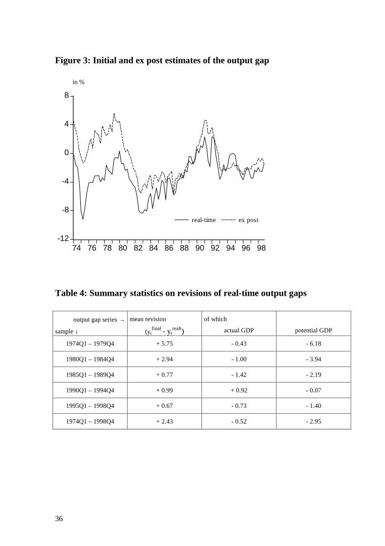
Figure 3: Initial and ex post estimates of the output gap

in %

Table 4: Summary statistics on revisions of real-time output gaps

output gap series →

sample ↓

mean revision

(ytfinal - yt

realt)of which

actual GDP potential GDP

1974Q1 – 1979Q4 + 5.75 - 0.43 - 6.18

1980Q1 – 1984Q4 + 2.94 - 1.00 - 3.94

1985Q1 – 1989Q4 + 0.77 - 1.42 - 2.19

1990Q1 – 1994Q4 + 0.99 + 0.92 - 0.07

1995Q1 – 1998Q4 + 0.67 - 0.73 - 1.40

1974Q1 – 1998Q4 + 2.43 - 0.52 - 2.95

-12

-8

-4

0

4

8

74 76 78 80 82 84 86 88 90 92 94 96 98

real-time ex post

36

Figure 4: Initial and ex post estimates of the change in the output gap

Change from previous year in %, quarterly data

-8

-6

-4

-2

0

2

4

1975 1980 1985 1990 1995

initial estimates ex post estimates

Figure 5: Measurement errors of output gap and change in the gap

percentage points

-4

-2

0

2

4

6

8

1975 1980 1985 1990 1995

output gapchange in output gap

37

Table 5: Structure of the real-time data set for CPI inflation

Month ofPublication τ →

74/03 74/04 ... 95/09 95/10 ...

Reported forquarter t ↓

74/01 74/02

...

99/01

1972/11 π72/11 π72/11 π72/11 π72/11 ...

... ... ... ... ... ...

1973/12 π73/12 π73/12 π73/12 π73/12 ...

1974/01 π74/01 π74/01 π74/01 ...

1974/02 π74/02 π74/02 ...

1974/03 π74/03 ...

... ...

1992/01 π92/01 π92/01 π92/01 π92/01

... ... ... ... ...

1995/08 π95/08 π95/08 ... π95/08

1995/09 ... ... ... ... π95/09 ... π95/09

... ... ...

1998/12 . π98/12

38

Figure 6: Initial and ex post data on CPI inflation

Figure 7: Real-time inflation gaps - CPI versus output deflator

-2

0

2

4

6

8

1975 1980 1985 1990 1995

real-time ex post

Change from previous year in %, quarterly averages

-4

-3

-2

-1

0

1

2

3

4

5

1975 1980 1985 1990 1995

CPI output deflator

Change from previous year in %, quarterly values

39

Table 6: Medium-term price assumption 1975 - 1998

Year PriceAssumption

Year PriceAssumption

Year PriceAssumption

1975 5.0 1983 3.5 1991 2.0

1976 5.0 1984 3.0 1992 2.0

1977 3.5*/4.0** 1985 2.0 1993 2.0

1978 3.5 1986 2.0* 1994 2.0

1979 4.0 1987 2.0 1995 2.0

1980 4.0 1988 2.0 1996 2.0

1981 3.5-4.0 1989 2.0 1997 1.5-2.0

1982 3.5* 1990 2.0 1998 1.5-2.0

*Explicit reference to GNP deflator; **explicit reference to consumer price index.

Figure 8: Initial and ex post data on money growth (as measured bythe Bundesbank’s respective target variable)

-2

0

2

4

6

8

10

12

14

1975 1980 1985 1990 1995

real-time ex post

Change fromprevious year in %, quarterlyaverages

40

Tab

le 7

: Str

uctu

re o

f the

rea

l-tim

e da

ta se

t for

the

rate

of g

row

th o

f the

res

pect

ive

mon

etar

y ta

rget

var

iabl

e

Mon

th o

fPu

blic

atio

n τ →

74/1

074

/11

74/1

2...

87/1

288

/01

88/0

188

/02

...99

/01

99/0

299

/03

Rep

orte

d fo

rqu

arte

r t ↓

1969

/01

cbm

69/0

1cb

m69

/01

cbm

69/0

1

......

......

...

1974

/09

cbm

74/0

9cb

m74

/09

cbm

74/0

9...

1974

/10

cbm

74/1

0cb

m74

/10

...

1974

/11

cbm

74/1

1...

......

......

......

...

1987

/11

cbm

87/1

1cb

m87

/11

M3 8

7/11

M3 8

7/11

...

1987

/12

cbm

87/1

2M

3 87/

12M

3 87/

12...

1988

/01

M3 8

8/01

...

......

......

1998

/12

M3 9

8/12

M3 9

8/12

M3 9

8/12

41

Figure 9: Overnight and three-month interest rates in Germany (end-

of-quarter values)

Figure 10: The time pattern for i and ππππ

t t+1 t+2 t+3 t+4 t+5 t+6

πt+4

πt+5

πt+6

it

2

4

6

8

10

12

14

80 82 84 86 88 90 92 94 96 98

overnight 3-month

42

Table 8: Parameter estimates of the baseline reaction function with ex

post revised data

Estimation equation:

( ) ttTtTntntTntt QdciyEßEEi εργπππαρ +⋅++Ω+Ω−+Ω+−= −+++ 181)())(()()1( 1** 1)

Estimation period: 1979Q1 to 1998Q4, T=1999Q1, estimation method: GMM; HAC-robust standard errors inparentheses2)

n=4 n=5 n=6

α 3.79***

(0.28)

3.47***

(0.26)

3.38***

(0.24)

β 0.82**

(0.34)

1.43***

(0.32)

1.61***

(0.28)

γ 0.76***

(0.19)

0.53***

(0.15)

0.51***

(0.13)

ρ 0.81***

(0.02)

0.79***

(0.02)

0.81***

(0.02)

R² 0.95 0.95 0.95

SEE 0.55 0.59 0.55

J-stat (p-values) 0.78 0.86 0.87

Jarque Bera(p-values) 0.81 0.26 0.52

***(**/*) denotes significance at the 1% (5%/10%) level; values in brackets are robust standard errors.

1) To correct for extreme outliers in the residuals, it proved necessary to include a dummy variable in theestimations which is one in the first quarter of 1981 and zero otherwise. The dummy captures the jump in moneymarket rates which occurred in February 1981 when the Bundesbank replaced its “normal” lombard loans by anew special lombard facility which cost 3 percentage points more. See Bundesbank (1982), p. 5. 2) Theinstrument set includes the contemporary values of inflation and the price assumption (which were known topolicy makers at the end of each quarter) as well as four lags of each explanatory variable.

R²: adjusted coefficient of determination; SEE: standard error of the regression; J-stat: p-value of the J-statisticon the validity of overidentifying restrictions ; Jarque Bera: p-value of the Jarque Bera test of the normality ofresiduals.

43

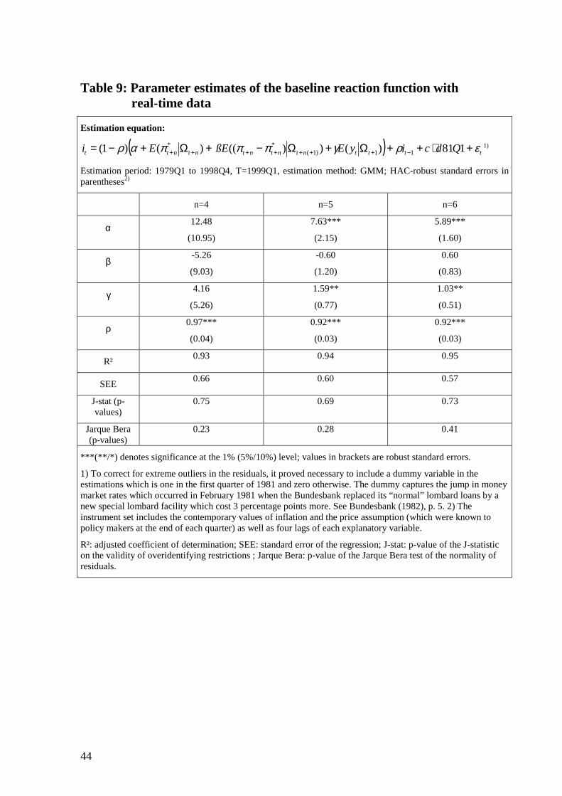
Table 9: Parameter estimates of the baseline reaction function withreal-time data

Estimation equation:

( ) ttttntntntntntt QdciyEßEEi εργπππαρ +⋅++Ω+Ω−+Ω+−= −+++++++ 181)())(()()1( 11)1(** 1)

Estimation period: 1979Q1 to 1998Q4, T=1999Q1, estimation method: GMM; HAC-robust standard errors inparentheses2)

n=4 n=5 n=6

α12.48

(10.95)

7.63***

(2.15)

5.89***

(1.60)

β-5.26

(9.03)

-0.60

(1.20)

0.60

(0.83)

γ4.16

(5.26)

1.59**

(0.77)

1.03**

(0.51)

ρ0.97***

(0.04)

0.92***

(0.03)

0.92***

(0.03)

R² 0.93 0.94 0.95

SEE 0.66 0.60 0.57

J-stat (p-values)

0.75 0.69 0.73

Jarque Bera(p-values)

0.23 0.28 0.41

***(**/*) denotes significance at the 1% (5%/10%) level; values in brackets are robust standard errors.

1) To correct for extreme outliers in the residuals, it proved necessary to include a dummy variable in theestimations which is one in the first quarter of 1981 and zero otherwise. The dummy captures the jump in moneymarket rates which occurred in February 1981 when the Bundesbank replaced its “normal” lombard loans by anew special lombard facility which cost 3 percentage points more. See Bundesbank (1982), p. 5. 2) Theinstrument set includes the contemporary values of inflation and the price assumption (which were known topolicy makers at the end of each quarter) as well as four lags of each explanatory variable.

R²: adjusted coefficient of determination; SEE: standard error of the regression; J-stat: p-value of the J-statisticon the validity of overidentifying restrictions ; Jarque Bera: p-value of the Jarque Bera test of the normality ofresiduals.

44

Table 10: Monetary targets and their implementation

in %

Target:growth of central bank money stock (1975-1987) or money stock M3 (from 1988)

Assumption Actual growth (roundedfigures)

Year in the courseof the year1

annualaverage

midyearreview

Q1, Q2 Q3, Q4 in thecourse ofthe year

annualaverage

1975 8 8 8 10

1976 8 9

1977 (6-7)2 8 6.5 6.5 9

1978 (5-7)2 8 6 6 11

1979 6-9 lower limit 7.5 6 6

1980 5-8 6 lower half 6.5 5.75 5

1981 4-7 5-5 ½ lower half 5.5 4.75 4

1982 4-7 4 ¾ upper half 6.253 6.25 6

1983 4-7 upper half 6.253 6.25 7

1984 4-6 5 5 5 5

1985 3-5 4 ½ 4 4 5

1986 3 ½ - 5 ½ 4 ½ 4.5 4.5 8

1987 3-6 4.5 4.5 8

1988 3-6 4.5 4.5 7

1989 about 5 just under 5 5 5 5

1990 4-6 about 5 5 5 6

1991 4-6 5/5 ¼ 3-5 4.54 4 5

1992 3 ½- 5 ½ 5-5 ¼ 4.5 4.5 9

1993 4 ½ - 6 ½ 6 5.5 5.5 7

1994 4-6 5 ½ 5 5 6

1995 4-6 5 ¾ 5 5 2

1996 4-7 5 ½ 5.5 5.5 8

19975 3 ½- 6 ½ 5 5 5

19985 3-6 4.5 4.5 6

1 Between the fourth quarter of the previous year and the fourth quarter of the current year; 1975: Dec. 1974 toDec. 1975. – 2 According to Annual Reports for 1977 and 1978. – 3 In 1982 and 1983, the Bundesbank made itclear that it targeted the upper half of the corridor at the beginning of the year. - 4 In 1991, the Bundesbank madeit clear that it targeted the lower half of the corridor at the beginning of the year. -5 Embedded in a two-yearorientation for 1997/1998 of about 5% per year.

45

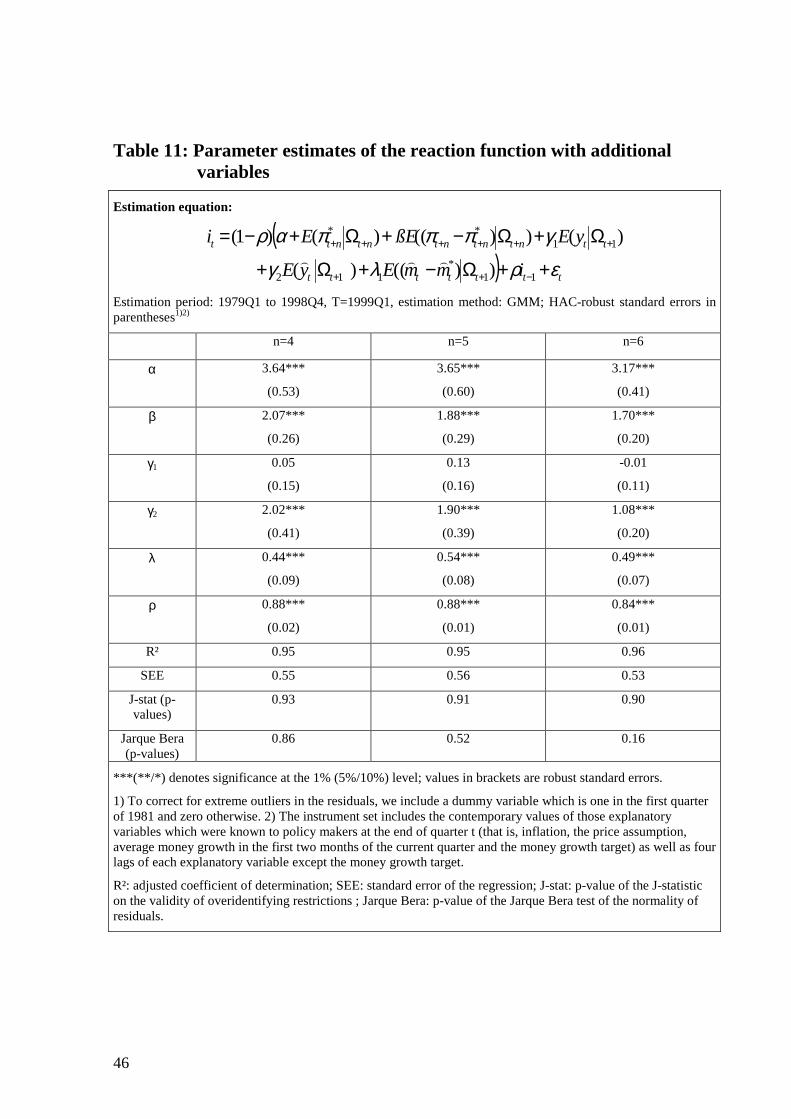
Table 11: Parameter estimates of the reaction function with additionalvariables

Estimation equation:

() ttttttt

ttntntntntntt

immEyE

yEßEEi

ερλγ

γπππαρ

++Ω−+Ω+

Ω+Ω−+Ω+−=

−++

++++++

11*

112

11**

))(() (

)())(()()1(

Estimation period: 1979Q1 to 1998Q4, T=1999Q1, estimation method: GMM; HAC-robust standard errors inparentheses1)2)

n=4 n=5 n=6

α 3.64***

(0.53)

3.65***

(0.60)

3.17***

(0.41)

β 2.07***

(0.26)

1.88***

(0.29)

1.70***

(0.20)

γ1 0.05

(0.15)

0.13

(0.16)

-0.01

(0.11)

γ2 2.02***

(0.41)

1.90***

(0.39)

1.08***

(0.20)

λ 0.44***

(0.09)

0.54***

(0.08)

0.49***

(0.07)

ρ 0.88***

(0.02)

0.88***

(0.01)

0.84***

(0.01)

R² 0.95 0.95 0.96

SEE 0.55 0.56 0.53

J-stat (p-values)

0.93 0.91 0.90

Jarque Bera(p-values)

0.86 0.52 0.16

***(**/*) denotes significance at the 1% (5%/10%) level; values in brackets are robust standard errors.

1) To correct for extreme outliers in the residuals, we include a dummy variable which is one in the first quarterof 1981 and zero otherwise. 2) The instrument set includes the contemporary values of those explanatoryvariables which were known to policy makers at the end of quarter t (that is, inflation, the price assumption,average money growth in the first two months of the current quarter and the money growth target) as well as fourlags of each explanatory variable except the money growth target.

R²: adjusted coefficient of determination; SEE: standard error of the regression; J-stat: p-value of the J-statisticon the validity of overidentifying restrictions ; Jarque Bera: p-value of the Jarque Bera test of the normality ofresiduals.

46

Table 12: Robustness of results for different horizons of the moneygrowth variable (with n=5)

Estimation equation:

() ttttttt

tttttttt

immEyE

yEßEEi

ερλγ

γπππαρ

++Ω−+Ω+

Ω+Ω−+Ω+−=

−++

++++++

11*

112

115*

555*

5

))(() (

)())(()()1(

Estimation period: 1979Q1 to 1998Q4, T=1999Q1, estimation method: GMM; HAC-robust standard errors inparentheses1)2)

money gap measured by

coefficients

↓↓↓↓

log money stock relative totarget path (CGG)

(annualised) six-month rate ofmoney growth relative to

target

annual rate of money growthrelative to target

α 3.32***

(0.53)

3.90***

(0.63)

3.65***

(0.60)

β 2.57***

(0.33)

2.13***

(0.40)

1.88***

(0.29)

γ1 -0.03

(0.14)

0.31*

(0.18)

0.13

(0.16)

γ2 1.70***

(0.34)

2.42***

(0.51)

1.90***

(0.39)

λ 0.59***

(0.10)

0.51***

(0.12)

0.54***

(0.08)

ρ 0.86***

(0.01)

0.89***

(0.02)

0.88***

(0.01)

R² 0.95 0.95 0.95

J-stat (p-values)

0.94 0.83 0.91

Jarque Bera(p-values)

0.46 0.42 0.52

***(**/*) denotes significance at the 1% (5%/10%) level; values in brackets are robust standard errors.

1) To correct for extreme outliers in the residuals, we include a dummy variable which is one in the first quarterof 1981 and zero otherwise. 2) The instrument set includes the contemporary values of those explanatoryvariables which were known to policy makers at the end of quarter t (that is, inflation, the price assumption,average money growth in the first two months of the current quarter and the money growth target) as well as fourlags of each explanatory variable except the money growth target.

R²: adjusted coefficient of determination; J-stat: p-value of the J-statistic on the validity of overidentifyingrestrictions ; Jarque Bera: p-value of the Jarque Bera test of the normality of residuals.

47

48

The following Discussion Papers have been published since 2003:

Series 1: Studies of the Economic Research Centre

January 2003 Testing mean-variance efficiency in CAPM Marie-Claude Beaulwith possibly non-gaussian errors: an Jean-Marie Dufourexact simulation-based approach Lynda Khalaf

January 2003 Finite-sample distributions ofself-normalized sums Jeong-Ryeol Kim

January 2003 The stock return-inflation puzzle andthe asymmetric causality in stock returns,inflation and real activity Jeong-Ryeol Kim

February 2003 Multiple equilibrium overnight ratesin a dynamic interbank market game Jens Tapking

February 2003 A comparison of dynamic panel dataestimators: Monte Carlo evidence andan application to the investment function Andreas Behr

March 2003 A Vectorautoregressive InvestmentModel (VIM) And Monetary Policy Joerg BreitungTransmission: Panel Evidence From Robert S. ChirinkoGerman Firms Ulf von Kalckreuth

March 2003 The international integration of moneymarkets in the central and east Europeanaccession countries: deviations from coveredinterest parity, capital controls and inefficien- Sabine Herrmanncies in the financial sector Axel Jochem

March 2003 The international integration offoreign exchange markets in the centraland east European accession countries:speculative efficiency, transaction costs Sabine Herrmannand exchange rate premiums Axel Jochem

49

March 2003 Determinants of German FDI: Claudia BuchNew Evidence from Jörn KleinertMicro-Data Farid Toubal

March 2003 On the Stability ofDifferent Financial Systems Falko Fecht

April 2003 Determinants of German ForeignDirect Investment in Latin American andAsian Emerging Markets in the 1990s Torsten Wezel

June 2003 Active monetary policy, passive fiscalpolicy and the value of public debt:some further monetarist arithmetic Leopold von Thadden

June 2003 Bidder Behavior in Repo Auctions Tobias Linzertwithout Minimum Bid Rate: Dieter NautzEvidence from the Bundesbank Jörg Breitung

June 2003 Did the Bundesbank React to Martin T. BohlStock Price Movements? Pierre L. Siklos

Thomas Werner

15 2003 Money in a New-Keynesian model Jana Kremerestimated with German data Giovanni Lombardo

Thomas Werner

16 2003 Exact tests and confidence sets for the Jean-Marie Dufourtail coefficient of α-stable distributions Jeong-Ryeol Kurz-Kim

17 2003 The Forecasting Performance of B R Craig, E Glatzer,German Stock Option Densities J Keller, M Scheicher

18 2003 How wacky is the DAX? The changing Jelena Stapfstructure of German stock market volatility Thomas Werner

50

1 2004 Foreign Bank Entry into Emerging Economies:An Empirical Assessment of the Determinantsand Risks Predicated on German FDI Data Torsten Wezel

2 2004 Does Co-Financing by Multilateral DevelopmentBanks Increase “Risky” Direct Investment inEmerging Markets? –Evidence for German Banking FDI Torsten Wezel

3 2004 Policy Instrument Choice and Non-Coordinated Giovanni LombardoMonetary Policy in Interdependent Economies Alan Sutherland

4 2004 Inflation Targeting Rules and Welfarein an Asymmetric Currency Area Giovanni Lombardo

5 2004 FDI versus cross-border financial services: Claudia M. BuchThe globalisation of German banks Alexander Lipponer

6 2004 Clustering or competition? The foreign Claudia M. Buchinvestment behaviour of German banks Alexander Lipponer

7 2004 PPP: a Disaggregated View Christoph Fischer

8 2004 A rental-equivalence index for owner-occupied Claudia Kurzhousing in West Germany 1985 to 1998 Johannes Hoffmann

9 2004 The Inventory Cycle of the German Economy Thomas A. Knetsch

10 2004 Evaluating the German Inventory CycleUsing Data from the Ifo Business Survey Thomas A. Knetsch

11 2004 Real-time data and business cycle analysisin Germany Jörg Döpke

12 2004 Business Cycle Transmission from the USto Germany – a Structural Factor Approach Sandra Eickmeier

51

13 2004 Consumption Smoothing Across States and Time: George M.International Insurance vs. Foreign Loans von Furstenberg

14 2004 Real-Time Estimation of the Output Gapin Japan and its Usefulness forInflation Forecasting and Policymaking Koichiro Kamada

15 2004 Welfare Implications of the Design of aCurrency Union in Case of Member Countriesof Different Sizes and Output Persistence Rainer Frey

16 2004 On the decision to go public: Ekkehart BoehmerEvidence from privately-held firms Alexander Ljungqvist

17 2004 Who do you trust while bubbles grow and blow?A comparative analysis of the explanatory powerof accounting and patent information for the Fred Rambmarket values of German firms Markus Reitzig

18 2004 The Economic Impact of Venture Capital Astrid Romain, Brunovan Pottelsberghe

19 2004 The Determinants of Venture Capital: Astrid Romain, BrunoAdditional Evidence van Pottelsberghe

20 2004 Financial constraints for investors and thespeed of adaption: Are innovators special? Ulf von Kalckreuth

21 2004 How effective are automatic stabilisers?Theory and results for Germany and other Michael ScharnaglOECD countries Karl-Heinz Tödter

22 2004 Asset Prices in Taylor Rules: Specification, Pierre L. SiklosEstimation, and Policy Implications for the Thomas WernerECB Martin T. Bohl

52

23 2004 Financial Liberalization and BusinessCycles: The Experience of Countries in Lúcio Vinhasthe Baltics and Central Eastern Europe de Souza

24 2004 Towards a Joint Characterization ofMonetary Policy and the Dynamics ofthe Term Structure of Interest Rates Ralf Fendel

25 2004 How the Bundesbank really conducted Christina Gerberdingmonetary policy: An analysis based on Andreas Wormsreal-time data Franz Seitz

53

Series 2: Banking and Financial Supervision

1 2003 Measuring the Discriminative Power B. Engelmann,of Rating Systems E. Hayden, D. Tasche

2 2003 Credit Risk Factor Modeling and A. Hamerle,the Basel II IRB Approach T. Liebig, D. Rösch

1 2004 Forecasting Credit Portfolio Risk A. Hamerle,T. Liebig, H. Scheule

2 2004 Systematic Risk in Recovery Rates –An Empirical Analysis of US Corporate Klaus DüllmannCredit Exposures Monika Trapp

3 2004 Does capital regulation matter for bank Frank Heidbehaviour? Evidence for German savings Daniel Porathbanks Stéphanie Stolz

Visiting researcher at the Deutsche Bundesbank

The Deutsche Bundesbank in Frankfurt is looking for a visiting researcher. Visitors shouldprepare a research project during their stay at the Bundesbank. Candidates must hold aPh D and be engaged in the field of either macroeconomics and monetary economics,financial markets or international economics. Proposed research projects should be fromthese fields. The visiting term will be from 3 to 6 months. Salary is commensurate withexperience.

Applicants are requested to send a CV, copies of recent papers, letters of reference and aproposal for a research project to:

Deutsche BundesbankPersonalabteilungWilhelm-Epstein-Str. 14

D - 60431 FrankfurtGERMANY

54