Complex Systems 3 (1989) 243-251

How the Lattice Gas Model for the Navier-StokesEquation Improves When aNew Speed is Added

Shiyi ChenHudong Chen

Gary D. DoolenCenter for Nonlinear Studies, Los Alamos National Lab oratory,

Los Alamos, NM 87545, USA

Abstract. The original lattice gas automaton model requires a den­sity-dependent rescaling of time, viscosity, and pressure in order toobtain the Navier-Stokes equation. Also, the corresponding equation­of-state contains an unphysical velocity dependence. We show that anextension of this model which includ es six additional par ticles with anew speed overcomes both problems to a large extent. The new modelconsiderably extends the ran ge of allowed Reynolds numb er.

1. Introduction

It has been shown theoretically and numerically by Fris ch , Hasslacher, andPomeau [1] and others [2-4] that the lattice gas or cellular automaton (CA) isan effective numerical technique for solving Navier-Stokes equation and manyother types of partial differ ential equations. The important properties of thelocal interaction between lattice gas particles and efficient memory utilizationmake the lattice gas an ideal method for massively parallel compute rs .

Most of the recent lattice gas studies of two-dimensional hydrodyn amicproblems are based on a hexagonal lattice in which the stress tensor isisotropic up to fourth order in the sp eed. Du e to both the discret enessof the lattice and the limited range of velociti es , the lattice gas model is notGalilean-invariant. The limitation of pr evious models to a single, nonzerospeed causes two problems.

The first problem is that g(n), the coefficient of the convective termin the Navier-Stokes momentum equation, is not equal to 1, as it shouldbe in a physical system. This problem can be overcome by a density­dependent rescaling of time, viscosity, and pr essure. This rescaling decreasesthe Reynolds number, requiring additional computational time and sto rage.

The second problem is that the equation-of-state depends on the macro­scopic speed in the form P = Po(n ,T) +PI (n, T)u2

. Here n is the particledensity, T is the temperature, and u is the field speed. Recently it has been

© 1989 Complex Systems Publications, Inc.

244 s. Cben, H. Cben, and G. Doolen

(2.1)

demonstrated that a nonzero value of PI in the equation-of-state can causeunphysical oscillations in kinetic energy decay [5J. All the previous mod­els have PI directly proportional to g(n). Thus PI = 0 implies g(n) = O.This means that one cannot overcome these two problems simultaneously forprevious models.

In this paper, we present one type of multispeed, multimass lattice gasmodel which allows g(n) = 1 and PI = 0 simultaneously. This model is anextension of the hexagonal lattice in two dimensions .

2. A general multispeed model

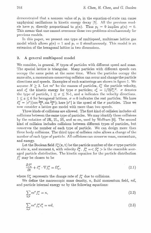
We consider, in general, N types of particles with different speed and mass.The spatial lattice is triangular. Many particles with different speeds canoccupy the same point at the same time. When the particles occupy thesame site, a momentum-conserving collision can occur and change the particledirections and speeds. Examples of such scatterings are shown in figure 1. Weas:~iUme N ;::: 3. Let mIT be the masses of particles, e: the particle velocity,and t:~ the kinetic energy for type a particles; t:~ = 1/2 1e';; 12

• a denotesthe type of particle, 1 ~ a ~ N-1, and a indicates the velocity directions.1 ~ a :S 6 for hexagonal lattices. a = 0 indicates the rest particles. We havee: = Ie" I(cos 2~a ,sin 2~a); here Ie"I is the speed of the a particles. Thus wenow consider a lattice gas model with more than two speeds.

Three kinds of collisions are allowed. The first kind of collision includes allcollisions between the same type of particles. We may identify these collisionsby the notation of 2R, 2L, 38, and so on, used by Wolfram [6J . The secondkind of collision includes collisions between different types of particles, butconserves the number of each type of particle. We can design more thanthree body collisions. The third type of collision rules allows a change of thenumber of each type of particle. All collisions can conserve mass, momentum,and energy.

Let the Boolean field S: (x, t) be the particle number of the a type particleat site x, and moment t, with velocity e:. f: =< S: > is the ensemble aver ­aged particle distribution. The kinetic equation for the particle distributionf: may be chosen to be

af: +e" . \1 po = f!"at a J a a'

where n~ represents the change rate of f: due to collisions.We define the macroscopic mass density, n, fluid momentum field, nil,

and particle internal energy ne by the following equations:

""' mIT po if' = nilL-t J a a ,a,"

(2.2)

(2.3)

How the Lattice Gas Model for the Navier-Stokes Equation Improves 245

( a )

(b )

( c )

Figure 1: Some collision rules for the 13-bit lattice gas model. T helength of the arrows is proportional to speed. Speed one particleshave a unit mass. Speed two particles have 1/2 unit mass. The leftside refers to the states before a collision. The right side refers tothe states after the collision. (a) describes collisions be tween sametype particles, (b ) describes collisions between different types, and (c)shows collisions which change the number of each type of particle .

I.:m" f: (e';; - it ) . (e';; - it ) = ne .a,(J

We may define the temperature T of the lattice gas as

(2.4)

(2.5)

where i is the number of degrees of freedom and kB is the Boltzmann constant.

246 S. Chen, H. Chen, and G. Doolen

The conservation of mass, momentum, and energy require the following:

a,"""' m"n"e: = 0L.-J aa ,a,"

a,"(2.6)

In order to obtain the hydrodynamic equation, we assume the local col­hsions cause the system to approach the local thermodynamic equilibriumstate. According to the Chapman-Enskog expansion method, the equilib­rium state corresponds to the zero order of collision term in kinetic equation(2.1), i.e, n~ (O) = O. This leads to the Fermi-Dirac equilibrium distribution

f"(0) = 1 (2 7)a 1 + exp [m"(a + ,8e'~ . it + I€~)]' .

where a, ,8, and I are Lagrange multipliers which are determined by thedefinitions (2.2), (2.3), and (2.4).

Taking moments of (2.1), we obtain the following continuity, momentum,and energy equations:

an _at + V' . nu = 0,

anit V'. n = 0at + ,

a(m) (_) _ pA ,,_~ + V' . nw + V'. q + : v tz = 0,

(2.8)

(2.9)

(2.10)

where n is the symmetric tensor of order 2, IT"/3 = La ,,, m" !::(e':),,(e':)/3, ifis the heat flux, (ij)" = La,,, m"I:! (e': - it)2(e': - it)", and P is the pressure

tensor, P"/3 = La,,, m" i:«: - it),,(e': - itkTo obtain the solutions for n, if, and P, we expand 1:(0) to third order

in speed, assuming litl ~ Cmin, and expand a = ao + al u2,,8 = ,80 + ,81 u2,and I = 10 + IIu2

. Here Cmin is the minimum nonzero "light" speed. T hevelocity expansion of 1:(0) then has the form

lau(O) da" - da"(l - da")[m" ,80e: . it +m" (al +111e:2

1)u2]

+ ~~ (1 - d~)(l - 2d~)m"2,802(e: . it)2

d~ (1 - d~)m",81 (e: . it)u2

+ d~(1 - d~)(l- 2d~)m"2,80(al +Ille:12 )u2

~d~(1- d~)(l - 6d~ + 6d~2)m"3,803(e: . it)3 + . . " (2.11)

where d~ is the equilibrium particle distribution when it = 0,

(2.12)

How the Lattice Gas Model for the Nevier-Stokes Equation Improves 247

Because d~ does not depend on a, we can simplify d~ = du and c~ = cu'T he coefficients /30 ' /31> a I, and 11 in equations (2.11) and (2.12) are functionsof nand e which will be det ermined from the definitions of (2.2), (2.3) , and(2.4).

For the models in which the rest particle does not have the internal energy,we can obtain

(2.13)

where o ",{3 is the Kronecker symbol , g(n, c) is the coefficient of the convectivete rm ,

(2.14)

and

(2.15)

where M is the number of distinct velocity directions and D is the spacedimension,

andn

PI = 2'(1 - g(n, c)).

(2.16)

(2.17)

In equat ion (2.17), note that PI = 0 when g(n , c) = 1. This very desirablecoincidence is the direct result of including an addit ional speed in the mod el.

Equation (2.16) is the equa t ion-of-state for the ideal gas .Up to O(u2

) , the heat flux vector can be writ ten

(2.18)

_ L" m" d,,(I-d,,)Ic"I'where h(n, c) - 2L"m"d,,(I-d,,)Ic"\2' - 2.

Note that FHP-I and FHP-II models are degenerat e cases of equations(2.14) and (2.16) . After simple algebra, we obtain g(n, c) = ~:::~ and c = ~

for FHP-I, and g(n, c) = ~~~~~~l and c = ¥for FHP-II. These resu lts agreewith reference [9].

Now we consider the isothermal incompressible fluid limi t in the abovemultispeed models. We want to recover th e Navier-Stokes equation with nounphysical te rms at some fixed temp eratures. Note that if e and n both areconstant, the energy equation is automatically satisfied. We know that massdensity n and energy c are defined by (2.2) and (2.4). T hus, for a given massdensity, we can vary the temperature by vary ing the ratios of different typesof particle to mass density k" = du/n . T he temp erature is det ermined by

248 S. Chen, H. Chen, and G. Doolen

these ratios . The quantities, d", we consider here are the equilibrium values,determined by the equation (2.12).

If all the particles are in statistical equilibrium, the collisions betweenthe different types of particles should satisfy the detailed balance condit ion.After eliminating 0:0 and 10 in (2.12), we have

(2.19)

which is required by the principle of the detailed balance. d; ~, x =mi«~ <j)' Y = m.«~ <k)' and z = ~)<j~<k + <i~<J Note here we have N + 1variables but only N equations. The internal energy is still a free parameter.We may add the equation of g(n, t) = 1, or equivalently, PI = 0 and askwhether physical solutions exist for these equations. The physical solutionsrequire the conditions l~d" ~ 0 and t m ar ~ t ~ O. Here (J" varies from 0 toN-l and t m ar is determined by the model geometry. For the physical solu t ionof equations , we may write d" = d,,(n) and t = t(n) . We show later thatphysical solutions exist.

Because the lattice gas model has density fluct uations, we cannot exactlysatisfy the equation g(n, t ) = 1. Instead, we can write down the velocitydependence of n = no + nl u2 and t = to + tlu2

• Consequently we haveg(n,t ) = 1 + O(u2

) and PI = O(u2) . One can show that these u2 corrections

contribute terms of order u4 to the Navier-Stokes equation. Hence the orderof accuracy of the Navier-Stokes equation is unchanged by corrections oforder u2 in the density and internal energy.

3 . A simple example: The three-speed model

To illustrate our theoretical results, we examine the three-speed, mul ti mas smodel. The particles have speeds 0, 1, and 2 and masses 3/2, 1, and 1/2respectively. The collisions between different types particles are given byfigure 1. Up to the second order of litl,we obtain the equilibrium distributionsdo, dl , and d2 and the energy e as a function of den sity n . We have fourvariables from the four equations,

3"ido +6dl +3d2 = n ,

3dl +6d2 = ne,

(1 - dl ) 2 = (1 - do)( 1 - d2 ) ,

dl do d2

nd l(1 - dd(1- 2dl ) + 2d2(1 - d2)(1 - 2d2 )

= 12[dl(1 - dl ) + d2(1 - d2 )j2. (3.1)

In figure 2, we show the numerical solution of do, dl , and d2 when n :=; 2.5.Other allowed physical solutions appear for 3 :=; n :=; 4.5 and 7 :=; n :=; 10.5.For other values of n, some d, becomes unphysically negative.

How the Lat tice Gas Model for the Navier-S tokes Equ ation Improves 249

-r--------------------...,.-§ci

~

a

t>"lj

ci

§

'"c

~§

a C0.0 0.5 1.0 1.5 2.0 2.5

n

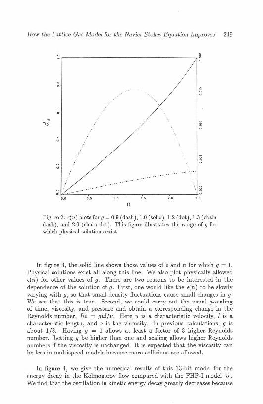
Figure 2: E(n) plots for 9 = 0.9 (dash), 1.0 (solid), 1.2 (dot), 1.5 (chaindash), and 2.0 (chain dot) . This figure illustrates the range of 9 forwhich physical solutions exist .

In figure 3, the solid line shows those values of t and n for which 9 = 1.Physical solutions exist all along this line. We also plot physically allowedt(n) for other values of g. T here are two reasons to be interested in thedependence of the solution of g. First , one would like the t (n) to be slowlyvary ing with g , so that small density fluctuat ions cause sm all changes in g.We see that this is true. Second, we could carry out the usual g-scal ingof time, viscosity, and pressure and obtain a corresponding change in theReynolds number, Re = qul]« . Here u is a characteristic velocity, 1 is acharacteristic length, and v is the viscosity. In previous calculations, 9 isabout 1/3. Having 9 = 1 allows at least a factor of 3 higher Reynoldsnu mb er. Let ting 9 be higher than one and scaling allows higher Reyn oldsnumbers if the viscosity is un changed. It is expecte d that the viscosity canbe less in multi speed mod els be caus e more collisions are allowed.

In figure 4, we give the numerical results of this 13-bit model for theenergy decay in the Kolmogorov flow compared with the FHP-I model [5].We find that the oscillation in kine tic energy decay greatly decreases be cause

250 S. Chen, H. Chen, and G. Doolen

~

cr-- - - - - - - - - - - - - - -,

-------- -- ----'-'- ­ --_._._.-- '-'-

>-nfEowZw

--'tt:Z

'"W.... NZO

o0+- ....... ....... ....,... -10 .0 o.s 1.0 1.5 :Z.O 2.5

DENSITY

Figure 3: Equilibrium distributions for speed zero (solid), speed one(dash), and speed two (dot , right vertical coordinate) when g(n , E) =1. This figure demonstrates the existence of physical solutions wheng , the coefficient of the iI · 'Vii term, is unity.

PI equals to zero in the present model. The internal energy decay rate iswit hin three percent of the theoreti cal prediction.

4. Conclusions

The multispeed lattice gas automaton model is the simple extension of FHPlat ti ce gas mod el by adding mor e speeds. This method leads to thermohy­dr odynamic equations. One impor tant result of the additio nal flexibility isthat we can have g(n} = 1 and PI = 0 to second-order accuracy in the speedu . The expense of adding more bits to the model is offset by the increasein the allowed range of Reyn olds number. The extens ion of this work tothree-dimensional hydrodynamics is straightforward.

5. Acknowledgments

We thank U. Frisch, B. Hasslacher , M. Lee, and :D. Montgomery for helpfuldiscussions. T his work is supported by the U.S. Department of Energy atLos Alamos National Lab oratory.

How the Lattice Gas Model for the Navier-Stokes Equation Im proves 251

~-=----------------,

0 .0 500.0 lOOJ .OTIME

ISOO.O

Figure 4: The streamwise kinetic energy for Kolmogor ov flow. Uo =0.3 sin(y). The solid curve is the 13-bit result with n = 2.0 andf = 0.25. The dashed curve is the 6-bit result when n = 1.8 and e =0.5. The unphysical oscillation presented in the 6-bit resul t is reducedsignificantly in the 13-bit result because the u2 term in th e pressurehas been eliminated .

References

[1] U. Frisch, B. Hasslacher , and Y. Pomeau , Pliys, Rev. Let t., 56 (1986) 1505.

[2] D. Boghosian and D. Levermore, Complex Sy stems, 1 (1987) 17.

[3] T. Shimomura, Gary D. Doolen, B. Hasslacher , and C. Fu, Los AlamosScience special issue, 1987.

[4] H. Chen, S. Chen, Gary D. Doolen, and Y.C. Lee, Complex Sy stems, 2(1988) 259.

[5] J .P. Dahlburg, D. Montgom ery, and G. Doolen, Pliys. Rev. ,A36(1987)2471.

[6] S. Wolfram, J. Stat. Puys., 45 (1986) 471.

[7] T . Hatori and D. Mont gomery, Compl ex Sy stems , 1 (1987) 734.

[8] S. Chen, M. Lee, Gary D. Doolen, and K. Zhao, "A lat tice gas model wit htemp erature," Physics. D, 37 (1989) 42.

[9] D. d'Humieres and P. Lallemand , Complex Sys tems, 1 (1987) 599.