NBER WORKING PAPER SERIES

HOW THE WEALTH WAS WON:FACTORS SHARES AS MARKET FUNDAMENTALS

Daniel L. GreenwaldMartin Lettau

Sydney C. Ludvigson

Working Paper 25769http://www.nber.org/papers/w25769

NATIONAL BUREAU OF ECONOMIC RESEARCH1050 Massachusetts Avenue

Cambridge, MA 02138April 2019, Revised April 2021

This paper supplants an earlier paper entitled "Origins of Stock Market Fluctuations." We are grateful to Simcha Barkai, John Y. Campbell, Andrea Eisfeldt, Valentin Haddad, Ralph Koijen, Edward Nelson, Annette Vissing-Jorgensen, and Mindy Xiaolan for helpful comments, and to seminar participants at the October 2020 NBER EF&G meeting, 2020 Women in Macro conference, the 2021 American Finance Association meetings, the January 2021 NBER Long Term Asset Management conference, the Federal Reserve Board, the Harvard University economics department, the HEC Paris Finance department, the Ohio State University Fisher College of Business, the University of California Berkeley Haas School of Business, the University of Chicago Booth School of Business, the University of Michigan Ross School of Business, and the University of Minnesota Carlson School for helpful comments. The views expressed herein are those of the authors and do not necessarily reflect the views of the National Bureau of Economic Research.

NBER working papers are circulated for discussion and comment purposes. They have not been peer-reviewed or been subject to the review by the NBER Board of Directors that accompanies official NBER publications.

© 2019 by Daniel L. Greenwald, Martin Lettau, and Sydney C. Ludvigson. All rights reserved. Short sections of text, not to exceed two paragraphs, may be quoted without explicit permission provided that full credit, including © notice, is given to the source.

How the Wealth Was Won: Factors Shares as Market Fundamentals Daniel L. Greenwald, Martin Lettau, and Sydney C. Ludvigson NBER Working Paper No. 25769April 2019, Revised April 2021JEL No. G0,G12,G17

ABSTRACT

Why do stocks rise and fall? From 1989 to 2017, $34 trillion of real equity wealth (2017:Q4 dollars) was created by the U.S. corporate sector. We estimate that 44% of this increase was attributable to a reallocation of rewards to shareholders in a decelerating economy, primarily at the expense of labor compensation. Economic growth accounted for just 25%, followed by a lower risk price (18%), and lower interest rates (14%). The period 1952 to 1988 experienced less than one third of the growth in market equity, but economic growth accounted for more than 100% of it.

Daniel L. GreenwaldMIT Sloan School of Management100 Main Street, E62-641Cambridge, MA 02142 dlg@mit.edu

Martin LettauHaas School of BusinessUniversity of California, Berkeley545 Student Services Bldg. #1900Berkeley, CA 94720-1900and CEPRand also NBERlettau@haas.berkeley.edu

Sydney C. LudvigsonDepartment of EconomicsNew York University19 W. 4th Street, 6th FloorNew York, NY 10002and NBERsydney.ludvigson@nyu.edu

1 Introduction

Why do stocks rise and fall? Surprisingly little academic research has focused directly on this

question.1 While much of the literature has concentrated on explaining expected quarterly

or annual returns, this paper takes a longer view and considers the economic forces that have

driven the total value of the market over the post-war era. According to textbook economic

theories, the stock market and the broader economy should share a common trend, implying

that the same factors that boost economic growth are also the key to rising equity values

over longer periods of time.2 In this paper, we directly test this paradigm.

Some basic empirical facts serve to motivate the investigation. While the U.S. equity

market has done exceptionally well in the post-war period, this performance has been highly

uneven over time, even at long horizons. For example, real market equity of the U.S. corpo-

rate sector grew at an average rate of 7.5% per annum over the last 29 years of our sample

(1989 to 2017), compared to an average of merely 1.6% over the previous 29 years (1966

to 1988). At the same time, growth in the value of what was actually produced by the

corporate sector has displayed a strikingly different temporal pattern. While real corporate

net value added grew at a robust average rate of 3.9% per annum from 1966 to 1988 amid

anemic stock returns, it averaged much lower growth of only 2.6% from 1989 to 2017 even

as the stock market was booming. This multi-decade disconnect between growth in market

equity and output presents a difficult challenge to theories in which economic growth is the

key long-run determinant of market returns.

One potential resolution of this puzzle is to posit that economic fundamentals such as

cash flows may be relatively unimportant for the value of market equity, with discount rates

driving the bulk of growth even at long horizons. In this paper we entertain an alternative

hypothesis motivated by an additional set of empirical facts. Within the total pool of net

value added produced by the corporate sector, only a relatively small share — averaging

12.3% in our sample — accrues to the shareholder in the form of after-tax profits. Impor-

tantly, however, this share varies widely and persistently over time, fluctuating from less

than 8% to nearly 20% over our sample. This suggests that swings in the profit share are

strong enough to cause large and long-lasting deviations between cash flows and output. If

so, growth in market equity could diverge from economic growth for an extended period of

time, even when valuations are largely driven by fundamental cash flows. Indeed, while the

1We refer here to the question of what determines the level of equity values, as opposed to studyingdeterminants of the price-dividend ratio or expected returns.

2This tenet goes back to at least Klein and Kosobud (1961), followed by a vast literature in macroeconomictheory that presumes balanced growth among economic aggregates over long periods of time. For a morerecent variant, see Farhi and Gourio (2018).

2

Figure 1: Stock Market Ratios (Scale: 1989:Q1 = 1)

0.0

0.5

1.0

1.5

2.0

2.5

3.0

3.5

4.0

1952 1955 1958 1961 1964 1967 1970 1973 1976 1979 1982 1985 1988 1991 1994 1997 2000 2003 2006 2009 2012 2015 2018

ME/GDP ME/C ME/NVA ME/E

1989.Q1 = 1

Notes: To make the units comparable, each series has been normalized to unity in 1989:Q1. The samplespans the period 1952:Q1-2018:Q2. ME: Corporate Sector Stock Value. E: Corporate Sector After-TaxProfits. GDP & C: Current Dollars GDP and personal consumption expenditures. NVA: Gross ValueAdded of Corporate Sector - Consumption of Fixed Capital.

1989-2017 period lagged the 1966-1988 period in economic growth, it exhibited growth in

corporate earnings of 5.1% per annum that far outpaced the average 1.8% earnings growth

of the previous period. Behind these trends are movements in the after-tax profit share of

output, which fell from 15.3% in 1966 to 8.9% in 1988, before rising again to 17.4% by the

end of 2017. These shifts are in turn made possible by a reverse pattern in labor’s share of

corporate output, which rises from 67.0% in 1966:Q1 to 72.4% in 1988:Q4, before reverting

to 67.7% by 2017:Q4.

The upshot of these trends is a widening chasm between the stock market and the broader

economy. This phenomenon is displayed in Figure 1, which plots the ratio of market equity

for the corporate sector to three different measures of aggregate economic activity: gross

domestic product, personal consumption expenditures, and net value added of the corporate

sector. Despite substantial volatility in these ratios, each is at or near a post-war high by

the end of 2017. Notably, however, the ratio of market equity to after-tax profits (earnings)

for the corporate sector is far below its post-war high.

What role, if any, might these trends have played in the evolution of the post-war stock

market? To translate these empirical facts into a quantitative decomposition of the post-war

growth in market equity, we construct and estimate a model of the U.S. equity market.

3

Although the specification of a model necessarily imposes some structure, our approach is

intended to let the data speak as much as possible. We do this by estimating a flexible

parametric model of how equities are priced that allows for influence from a number of

mutually uncorrelated latent factors, including not only factors driving productivity and

profit shares, but also independent factors driving risk premia and risk-free interest rates.

Equity in our model is priced, not by a representative household, but by a representative

shareholder, akin in the data to a wealthy household or large institutional investor. The

remaining agents supply labor, but play no role in asset pricing. Shareholder preferences

are subject to shocks that alter their patience and appetite for risk, driving variation in

both the equity risk premium and in risk-free interest rates. Our representative shareholder

consumes cash flows from firms, the variation of which is driven by shocks to the total rewards

generated by productive activity, but also by shocks to how those rewards are divided between

shareholders and other claimants. Our model is able to account for operating leverage effects

due to capital investment, implying that the cash flow share of output moves more than one-

for-one with the earnings share (the leverage effect), and that cash flow growth is more

volatile when the earnings share is low (the leverage risk effect).

We estimate the full dynamic model using state space methods, allowing us to precisely

decompose the market’s observed growth into these distinct component sources. The model

is flexible enough to explain the entirety of the change in equity values over our sample and

at each point in time. To capture the influence of our primitive shocks at different horizons,

we model each as a mixture of multiple stochastic processes driven by low and high frequency

variation. Because our log-linear model is computationally tractable, we are able to account

for uncertainty in both latent states and parameters using millions of Markov Chain Monte

Carlo draws. We apply and estimate our model using data on the U.S. corporate sector over

the period 1952:Q1-2017:Q4.

Our main results may be summarized as follows. First, we find that neither economic

growth, risk premia, nor risk-free interest rates has been the foremost driving force behind

the market’s sharp gains over the last several decades. Instead, the single most important

contributor has been a string of factor share shocks that reallocated the rewards of production

without affecting the size of those rewards. Our estimates imply that the realizations of

these shocks persistently reallocated rewards to shareholders, to such an extent that they

account for 44% of the market increase since 1989. Decomposing the components of corporate

earnings reveals that the vast majority of this increase in the profit share came at the expense

of labor compensation.

Second, while equity values were also boosted since 1989 by persistent declines in the

market price of risk, and in the real risk-free rate, these factors played smaller roles quan-

4

titatively, contributing 18% and 14%, respectively, to the increase in the stock market over

this period.

Third, growth in the real value of corporate sector output contributed just 25% to the

increase in equity values since 1989 and 54% over the full sample. By contrast, while economic

growth accounted for more than 100% of the rise in equity values from 1952 to 1988, this 37

year period created less than a third of the growth in equity wealth generated over the 29

years from 1989 to the end of 2017.

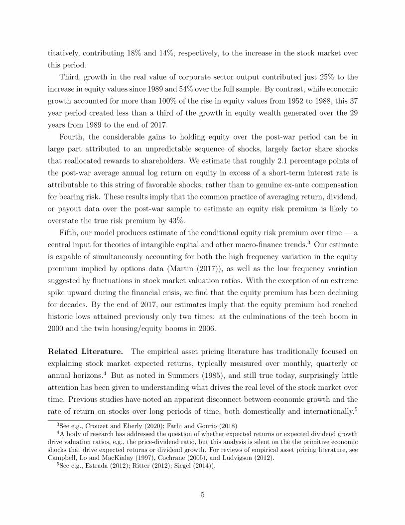
Fourth, the considerable gains to holding equity over the post-war period can be in

large part attributed to an unpredictable sequence of shocks, largely factor share shocks

that reallocated rewards to shareholders. We estimate that roughly 2.1 percentage points of

the post-war average annual log return on equity in excess of a short-term interest rate is

attributable to this string of favorable shocks, rather than to genuine ex-ante compensation

for bearing risk. These results imply that the common practice of averaging return, dividend,

or payout data over the post-war sample to estimate an equity risk premium is likely to

overstate the true risk premium by 43%.

Fifth, our model produces estimate of the conditional equity risk premium over time — a

central input for theories of intangible capital and other macro-finance trends.3 Our estimate

is capable of simultaneously accounting for both the high frequency variation in the equity

premium implied by options data (Martin (2017)), as well as the low frequency variation

suggested by fluctuations in stock market valuation ratios. With the exception of an extreme

spike upward during the financial crisis, we find that the equity premium has been declining

for decades. By the end of 2017, our estimates imply that the equity premium had reached

historic lows attained previously only two times: at the culminations of the tech boom in

2000 and the twin housing/equity booms in 2006.

Related Literature. The empirical asset pricing literature has traditionally focused on

explaining stock market expected returns, typically measured over monthly, quarterly or

annual horizons.4 But as noted in Summers (1985), and still true today, surprisingly little

attention has been given to understanding what drives the real level of the stock market over

time. Previous studies have noted an apparent disconnect between economic growth and the

rate of return on stocks over long periods of time, both domestically and internationally.5

3See e.g., Crouzet and Eberly (2020); Farhi and Gourio (2018)4A body of research has addressed the question of whether expected returns or expected dividend growth

drive valuation ratios, e.g., the price-dividend ratio, but this analysis is silent on the the primitive economicshocks that drive expected returns or dividend growth. For reviews of empirical asset pricing literature, seeCampbell, Lo and MacKinlay (1997), Cochrane (2005), and Ludvigson (2012).

5See e.g., Estrada (2012); Ritter (2012); Siegel (2014)).

5

But these works have not provided a model and evidence on the economic foundations of

this disconnect or on the alternative forces that have driven the market in post-war U.S.

data, a gap our study is intended to fill.6

In this regard, the two papers closest to this one are Lettau and Ludvigson (2013) and

our previous work entitled “Origins of Stock Market Fluctuations,” (Greenwald, Lettau and

Ludvigson (2014), hereafter GLL), which this paper supplants. Lettau and Ludvigson (2013)

was a purely empirical exercise that showed under a natural rotation scheme, shocks from

a VAR that push labor income and asset prices in opposite directions explain much of the

long-term trend in stock wealth. GLL expanded on this analysis by demonstrating that

a calibrated model could reproduce many of these VAR results. At the same time, neither

paper undertook a complete structural estimation of an equity pricing model, and thus could

not directly decompose movements in market valuations into fundamental structural forces.

Compared to GLL, the model in this paper is both richer and more flexible in terms of its

state variables and its cash flow process, is directly estimated on the time series rather than

calibrated, and produces a period-by-period accounting of the drivers of market equity.7

Like GLL and Lettau, Ludvigson and Ma (2018), the model of this paper adopts a

heterogeneous agent perspective characterized by “shareholders,” who hold the economy’s

financial wealth and consume capital income, and “workers” who finance consumption out

of wages and salaries. This choice is motivated by the empirical observation: the top 5%

of the stock wealth distribution owns 76% of the stock market value (and earns a relatively

small fraction of income from labor compensation), while around half of households have no

direct or indirect ownership of stocks at all.8 In this sense our model relates to a classic older

literature emphasizing the importance for stock pricing of limited stock market participation

and heterogeneity.9 We add to this literature by demonstrating the relevance of frameworks

in which investors are concerned about shocks that have opposite effects on labor and capital.

6One exception is Lansing (2021), a paper subsequent to the initial draft of our work, who also estimatesa model to exactly match and decompose macroeconomic and financial time series data, and emphasizes therole of sentiment.

7The older GLL paper solves a fully nonlinear model in place of an approximate log-linear model, demon-strating that the results in this paper are robust to allowing for these nonlinearities.

8Source: 2016 Survey of Consumer Finances (SCF). In the 2016 SCF, 52% of households report owningstock either directly or indirectly. Stockowners in the top 5% of the net worth distribution had a medianwage-to-capital income ratio of 27%, where capital income is defined as the sum of income from dividends,capital gains, pensions, net rents, trusts, royalties, and/or sole proprietorship or farm. Even this low numberlikely overstates traditional worker income for this group, since the SCF and the IRS count income paid inthe form of restricted stock and stock options as “wages and salaries.” Executives who receive substantialsums of this form would be better categorized as “shareholders” in the model below, rather than as “workers”who own no (or very few) assets.

9See e.g., Mankiw (1986), Mankiw and Zeldes (1991), Constantinides and Duffie (1996), Vissing-Jorgensen(2002), Ait-Sahalia, Parker and Yogo (2004), Guvenen (2009), and Malloy, Moskowitz and Vissing-Jorgensen(2009).

6

Besides Lettau and Ludvigson (2013), GLL, and Lettau et al. (2018), a growing body of

literature considers the role of redistributive shocks in asset pricing or macro models, most

in representative agent settings.10 In addition to our main distinguishing contribution that

we pursue a quantitative decomposition of the drivers of equity values over time using an

estimated structural model, we differ from this literature in our treatment of equity risk

and pricing. In this literature, labor compensation is a charge to claimants on the firm and

therefore a source of cash-flow variation in stock and bond markets, but typically imply that

a variant of the consumption CAPM using aggregate consumption still prices equity returns,

implying that these frameworks cannot not account for the evidence in Lettau et al. (2018)

that the capital (i.e., nonlabor) share of aggregate income is a strongly priced risk factor. In

contrast, our framework allows these redistributive shocks to influence not only cash flows

but also the quantity of risk faced by investors.11

Our work is also closely related to papers studying the sources of macroeconomic and

financial transitions over time. Farhi and Gourio (2018) extend a representative agent neo-

classical growth model to allow for time varying risk premia, and find a large role for rising

market power in the high returns to equity over the last 30 years, similar to our findings

regarding the importance of the factor share shock. Corhay, Kung and Schmid (2018) find

a similar result that they likewise attribute to market power using a rich model of the firm

investment margin. An appealing feature of these approaches is that they specify a struc-

tural model of production that takes a firm stand on the sources of variation in the earnings

share. In contrast, our modeling and estimation approach is designed to quantify what role

the earnings share has played in stock market fluctuations, without requiring us to take a

stand on the structural model that may have produced those equilibrium observations. As a

result, we are able to explain the full transition dynamics of the data period-by-period, while

Farhi and Gourio (2018) and Corhay et al. (2018) compare their richer production models

only across different steady states. We view this work as complementary, but discuss the

important implications of these differing methodological approaches further below.

Our work also relates to the literature estimating log-affine SDFs in reduced form.12

These works describe the evolution of the state variables and the SDF in purely statistical

10See e.g., Danthine and Donaldson (2002), Favilukis and Lin (2016, 2013, 2015), Gomez (2016), Marfe(2016), Farhi and Gourio (2018).

11The factors share element of our paper is also related to a separate macroeconomic literature that exam-ines the long-run variation in the labor share (e.g., Karabarbounis and Neiman (2013), and the theoreticalstudy of Lansing (2014)). The factors share findings in this paper also echo those from previous studiesthat use very different methodologies but find that returns to human capital are negatively correlated withthose to stock market wealth (Lustig and Van Nieuwerburgh (2008); Lettau and Ludvigson (2009); Chen,Favilukis and Ludvigson (2014))).

12See e.g., Ang and Piazzesi (2003), Bekaert, Engstrom and Xing (2009), Dai and Singleton (2002), Duffieand Kan (1996), Lustig, Van Nieuwerburgh and Verdelhan (2013).

7

terms, for example using a freely estimated vector autoregression (VAR) for state dynamics.

While less statistically flexible, our work features more economic structure, using separate

and mutually uncorrelated fundamental components, as well as parametric restrictions on the

SDF exposures obtained from theory, such as the leverage risk effect. This structure allows

a much clearer interpretation of the drivers of asset prices. For example, unlike VAR-based

models, which face the difficult task of transforming reduced-form residuals into identified

structural shocks, our model allows us to directly read off the contribution of each latent

state. We thus complement this literature by providing economic insight on the economic

sources of market fluctuations, particularly the role of factor shares.

Our study further connects with a large body on work contrasting the role of expected

dividend growth vs. discount rates in driving valuation ratios.13 Our emphasis on deter-

minants of cash flows (i.e., the earnings share) as a key driver of valuations differs from

these papers, which emphasize the role of discount rates, largely because we ask a different

question. While this literature finds that cash flows have little impact on the value of equity

relative to dividends, we focus on the value of equity relative to output. Because shifts in

the earnings share work precisely by driving a wedge between the earnings/payouts of the

corporate sector and its output, we do not view any contradiction between our results.

Last, we link to the broad literature that endogenizes equity risk premia based on the

consumption processes of its , by providing a new mechanism through the leverage risk

effect.14 This mechanism shares a deep similarity to the habit specification of Campbell

and Cochrane (1999), but is driven by variation in earnings relative to an external target

(reinvestment), rather than variation in aggregate consumption relative to an external target

(habit). This approach thus offers novel quantitative and empirical implications for variation

in risk premia over time that differ from consumption-based mechanisms.

Overview. The rest of this paper is organized as follows. Section 2 describes the theoretical

model. Section 3 presents the data. Section 4 describes our estimation procedure. Section 5

presents our findings. Section 6 considers robustness and extensions. Section 7 concludes.

2 The Model

This section presents our structural model of the equity market. Throughout this exposition,

lowercase letters denote variables in logs, while bolded symbols represent vectors or matrices.

13See e.g., Campbell and Shiller (1989), Cochrane (2011).14See e.g., Bansal and Yaron (2004), Barro (2009), Campbell and Cochrane (1999), Campbell, Pflueger

and Viceira (2014), Constantinides and Duffie (1996), Wachter (2013).

8

Demographics The economy is populated by a representative firm that produces aggre-

gate output, and two types of households. The first type are “shareholders” who typify

owners of most equity wealth in the U.S. (i.e., wealthy households or institutional investors).

They may borrow and lend among themselves in the risk-free bond market. The second type

are hand-to-mouth “workers” who finance consumption out of wages and salaries.15

Productive Technology Output is produced under a constant returns to scale process:

Yt = AtNαt K

1−αt , (1)

where At is a mean zero factor neutral total factor productivity (TFP) shock, Nt is the

aggregate labor endowment (hours times a productivity factor) and Kt is input of capital,

respectively. Workers inelastically supply labor to produce output. We seek a solution in

which capital grows deterministically at a gross rate G = exp(g), while labor productivity

grows deterministically at the same rate. Hours of labor supplied are fixed and normalized

to unity, so Nt = Gt. Taken together, these assumptions imply that

Yt = At(GtK0)α(Gt)1−α = AtG

tKα0 (2)

where K0 is the fixed initial value of the capital stock.

Factor Shares Once output is produced, it is divided among the various factors of pro-

duction and other entities. We define earnings (after-tax profits) as Et = StYt, where the

earnings share St represents the fraction of total output that accrues to shareholders in the

form of earnings, arising from both foreign and domestic operations. The remaining fraction

1 − St of output accrues to workers in the form of labor compensation, to the government

in the form of tax payments, and to debtholders in the form of interest payments. In our

estimation, we assume an exogenous process for St that does not directly distinguish between

shifts in these components, but return to analyze their separate roles in Section 5.5. For

now, we note that most variation in St is driven by the labor share of domestic value added.

15This stylized assumption is motivated in the U.S. data by the high concentration of top wealth shares,the evidence that the wealthiest earn the overwhelming majority of their income from ownership of assetsor firms, and finding households outside of the top 5% of the stock wealth distribution own far less financialwealth of any kind. In the 2016 SCF, the median household in the top 5% of the stock wealth distributionhad $2.97 million in nonstock financial wealth. By comparison, households with no equity holdings hadmedian nonstock financial wealth of $1,800, while all households (including equity owners) in the bottom95% of the stock wealth distribution had median nonstock financial wealth of $17,480. Additional evidenceis presented in Lettau, Ludvigson and Ma (2019).

9

Investment and Payout Technology. The firm makes cash payments to shareholders,

equal to earnings net of new investment. We assume that attaining balanced growth in

capital requires the firm to invest a fixed fraction ω of its output beyond replacing depreciated

capital. We view this as a parsimonious approximation to a richer model with time-varying

investment, which allows us to solve the model in closed form without tracking the capital

stock or solving the optimal investment problem, and provide additional support for this

assumption in Appendix A.6.16 Cash flows to shareholders consist of the remaining portion

of earnings net of this reinvestment:

Ct = Et − ωYt = (St − ω)Yt. (3)

The variable Ct is net payout, defined as net dividend payments minus net equity issuance.

It encompasses any cash distribution to shareholders including share repurchases, which have

become the dominant means of returning cash to shareholders in the U.S. For brevity, we

refer to these payments simply as “cash flows.”

Importantly, (3) implies that, since the cash flow share of output is equal to the earnings

share minus a constant reinvestment share, the volatility of cash flow growth is amplified

relative to earnings share growth — a form of operating leverage. For a numerical example,

if ω = 6%, then an increase in the earnings share St from 12% to 18% increases the cash flow

share from 6% to 12%. As a result, proportional growth in the cash flow share is twice as

large as proportional growth in the earnings share, a phenomenon that we call the leverage

effect. We note that this leverage effect should hold on average even if the reinvestment

share is not exactly constant, under the natural assumption that in the long run investment

is proportional to output rather than earnings.

Preferences. Let Csit denote the consumption of an individual stockholder indexed by i at

time t. Identical shareholders maximize the function

U0 = E∞∑t=0

t∏k=0

βku (Csit) , u (Cs

it) =(Cs

it)1−xt−1

1− xt−1

(4)

where E denotes the expectation operator. This specification effectively corresponds to power

utility preferences with a time-varying price of risk xt, and a time-varying time discount

factor βt. Since shareholders perfectly insure idiosyncratic risk, shareholder consumption Cit

16Jermann (1998) demonstrates that generating realistic asset pricing moments in production economiesrequires very large investment adjustment costs. Our investment process can be seen as a limiting case inwhich any deviation from this investment plan is infinitely costly.

10

is identically equal to aggregate cash flows Ct.17 At the same time, because firm cash flows

are only a subset of total economy-wide consumption, redistributive shocks to st that shift

the share of income between labor and capital shift shareholder consumption are a source of

systematic risk for asset owners. This implication has been explored by Lettau et al. (2019)

who study risk pricing in a large number of cross-sections of return premia.

Aggregating over shareholders, equities are priced by the stochastic discount factor of a

representative shareholder, taking the form

Mt+1 = βt

(Ct+1

Ct

)−xt(5)

This specification is a generalization of the SDFs considered in previous work, (e.g., Campbell

and Cochrane (1999) and Lettau and Wachter (2007)). As in these models, the preference

shifters (xt, βt) are taken as exogenous processes (akin to an external habit) that are the

same for each shareholder. We now discuss each of these items in turn.

Beginning with the risk price xt, we allow this variable to fluctuate stochastically over

time. Since an SDF always reflects both preferences and beliefs, an increase in xt may be

thought of as either an increase in effective risk aversion or an increase in pessimism about

shareholder consumption. Thus, xt may occasionally go negative, reflecting the possibility

that investors sometimes behave in a confident or risk tolerant manner.18

Shareholder preferences are also subject to an exogenous shifts in the subjective discount

factor βt. As is well known, applying a realistic level of variation in the risk price while

holding the time discount factor fixed would generate counterfactually high volatility in the

risk-free rate. Instead, following Ang and Piazzesi (2003), we specify βt as

βt =exp(−δt)

Et exp (−xt∆ct+1).

where ∆ct+1 represents log cash flow growth. This specification implies

EtMt+1 = exp(−δt) (6)

ensuring that the log risk-free rate exactly follows an exogenous stochastic process δt at all

17This need not imply that individual shareholders are hand-to-mouth households. They may trade anarbitrary set of assets with each other, including a complete set of state contingent contracts. Becausethey perfectly share any identical idiosyncratic risk with other shareholders they each consume per capitaaggregate shareholder cash flows Ct at equilibrium. See the Appendix for a stylized model.

18This does not imply a negative unconditional equity risk premium. Investors in the model occasionallybehave in a risk tolerant manner while still being averse to risk on average. Indeed, our estimates reportedbelow imply a substantial positive mean equity premium.

11

times, regardless of the values for the other state variables of the economy.

2.1 Model Solution and Parameterization

Exogenous Processes. Our model has four sets of exogenous processes that drive at, st, xt,

and δt, respectively. We specify TFP as a random walk in logs

∆at+1 = εa,t+1, εa,t+1iid∼ N(0, σ2

a).

Substituting into (2), we obtain

∆yt+1 = g + εa,t+1.

For the remaining latent states, we specify each as the sum of two components, each of which

are in turn specified as an independent AR(1) process:

st = s+ 1′st, st+1 = Φsst + εs,t+1, εs,t+1iid∼ N(0,Σs),

xt = x+ 1′xt, xt+1 = Φxxt + εx,t+1, εx,t+1iid∼ N(0,Σx),

δt = δ + 1′δt, δt+1 = Φδδt + εδ,t+1, εδ,t+1iid∼ N(0,Σδ)

where st, xt, and δt are 2× 1 vectors, Φs,Φx, and Φδ are 2× 2 diagonal matrices, and tildes

indicate that the latent state vectors are demeaned.

We choose this two-component mixture specification for each process to allow the model

to flexibly capture both high and low frequency variation in the latent states. Since equity

gives its owners access to profits for the lifetime of the firm, it is a heavily forward looking

asset that is much more influenced by persistent rather than transitory fluctuations. As a

result, our specification allows the model to accurately capture both low frequency move-

ments that have greater impact on equity prices, as well as higher frequency movements

that have a smaller impact on equity prices but may nonetheless drive much of the variation

in the observable series. Correspondingly, we refer to the components of each latent state

vector as the high or low frequency component, so that e.g., diag(Φs) = (φs,LF , φs,HF ) with

φs,LF > φs,HF .

Stacking this system yields the transition equation

zt+1 = Φzt + εt+1, εiid∼ N(0,Σ) (7)

12

for

zt =

st

xt

δt

∆at

, Φ =

Φs 0 0 0

0 Φx 0 0

0 0 Φδ 0

0 0 0 0

, εt =

εs,t

εx,t

εδ,t

εa,t

, Σ =

Σs 0 0 0

0 Σx 0 0

0 0 Σδ 0

0 0 0 σ2a

, (8)

where zt is the state vector for this economy.19

Log-Linearization. We seek a specification that allows an analytical, log-linear solution

for the price-dividend ratio. This solution requires three approximations: (i) a log-linear

approximation of the equity return, (ii) a log-linear approximation of cash flow growth, and

(iii) a second-order perturbation of the log SDF that allows for linear terms in the states

and shocks, as well as interactions between the states and shocks. We summarize these

approximations below, with full detail relegated to the appendix.

First, we approximate the return on equity

Rt+1 =Pt+1 + Ct+1

Pt.

where Pt denotes total market equity, i.e., price per share times shares outstanding. Following

Campbell and Shiller (1989), we approximate the log return as

rt+1 = κ0 + κ1pct+1 − pct + ∆ct+1, (9)

where κ1 = exp (pc) / (1 + exp (pc)), and κ0 = ln(exp (pc) + 1)− κ1pc.

Second, we log-linearize the log cash flow to output ratio ct − yt = log(St − ω) to obtain

ct − yt ' cy + ξ(st − s), ξ =S

S − ω

where cy = log(S − ω), and S is the average value of St. Differencing this relation and

rearranging yields

∆ct = ξ∆st + ∆yt. (10)

Importantly, for ω > 0 we have ξ > 1, so that changes in profit share map more than

19The i.i.d. shock εa,t is included the “state equation” (7) even though it is exactly pinned down by theobservable series ∆yt so that we can estimate its mean and variance, since these parameters influence ourasset pricing equations.

13

one-for-one into cash flows, preserving the leverage effect discussed above.

Finally, approximate our nonlinear SDF (5) using a perturbation around the steady state

that includes terms linear in zt and εt+1, as well as interactions between zt and εt+1. While

the complete solution and derivation can be found in the appendix, we present here the more

intuitive form

logMt+1 ' −δt − µt − xt (ξ∆st+1 + ∆yt+1)︸ ︷︷ ︸baseline cash flow risk

+ xξ(ξ − 1) (Et[st+1]− s) ∆st+1︸ ︷︷ ︸leverage risk effect

(11)

where µt is implicitly set to ensure a log risk-free rate of δt. The “baseline cash flow risk”

term represents the price of risk xt times the change in cash flows under the approximation

(10). The final leverage risk effect term is a second-order interaction, representing the fact

that the same shock to the earnings share εs,t+1 has a larger proportional impact on cash

flows when the current (and thus expected) earnings share is low. For example, if we again

assume ω = 6%, then increasing the earnings share from 8% to 10% would increase the cash

flow share of output by 100% (from 2% to 4%), while the same proportional increase in the

earnings share from 16% to 20% would only increase the cash flow share of output by 40%

(from 10% to 14%). The leverage risk effect captures this phenomenon, causing the SDF

to load more negatively on changes in profit shares when the expected profit share is low.

This leverage risk effect is very similar to the external habit mechanism of Campbell and

Cochrane (1999), but applied to earnings in place of consumption.

The specification (11) implies that changes in the profit share influence market valuations

by affecting both cash flows and risk premia. We view this risk premium channel as strongly

supported by the data. Figure 2 displays the time-series variation in the corporate sector log

earnings share of output, et−yt, alongside either the corporate sector log price earnings ratio

pt−et, or the Center for Research in Securities Prices (CRSP) log price-dividend ratio pt−dt,showing that these variables are positively correlated, particularly at lower frequencies. For

example, the correlation between et−yt and pt−dt is 69% for band-pass filtered components

of the raw series that retain fluctuations with cycles between 8 and 50 years.

A model with no correlation between the the earnings share and the price or quantity

of risk would instead unambiguously predict that pt − ct and pt − et should be negatively

correlated with the profit share. Because shocks to the profit share revert over time, they

influence prices (discounted forward-looking cash flows) less than current cash flows. Prices

in such a model will therefore rise less than proportionally with earnings in anticipation

of their eventual mean reversion, thereby resulting in a negative correlation between the

earnings share and valuation ratios — an intuition we formalize in our discussion of the

14

Figure 2: Earnings Share and Valuations

(a) vs. Price-Dividend Ratio (b) vs. Price-Earnings Ratio

Notes: ln(E/Y) denotes the logarithm of the after-tax profit (earnings) share of output for the corporatesector. ln(ME/E) is the log of the market equity-to-earnings ratio. ln(PD) is the log of the CRSP price-dividend. Each plot present the correlation between the series (levels) and the correlation of the cycle ofeach series obtained using a band pass filter that isolates cycles between 8 and 50 years. The sample spansthe period 1952:Q1-2017:Q4.

equilibrium conditions below. The positive correlation observed in the data instead implies

that persistently high earnings shares must coincide with a decline in expected future returns,

so that valuation ratios still rise even as earnings and shareholder payouts are rationally

expected to decline in the future.20

Equilibrium Stock Market Values. The first-order-condition for optimal shareholder

consumption implies the following Euler equation:

PtCt

= Et exp

[mt+1 + ∆ct+1 + ln

(Pt+1

Ct+1

+ 1

)]. (12)

The relevant state variables for the equilibrium pricing of equity are the vectors st, xt, δt.

We conjecture a solution to (12) taking the form

pct = A0 + A′sst + A′δδt + A′xxt. (13)

20If shocks to the earnings share improved shareholder fundamentals permanently, the model would implythat such shocks drive prices up proportionally with earnings, leaving valuation ratios unaffected and thecorrelation zero.

15

where pct = log(Pt/Ct) is the log price to cash-flow ratio. The solution, derived in Appendix

A.3, implies that the coefficients on these state variables take the form

A′s = −ξ[1′(I−Φs)− (1′Σs1)Γ′

][(I− κ1Φs)− κ1ξΣs1Γ′

]−1

A′x = −[(ξ2(1′Σs1) + σ2

a + κ1ξ(A′sΣs1)

)1′](I− κ1Φx)

−1

A′δ = −1′(I− κ1Φδ)−1

where the term

Γ′ = xξ(ξ − 1)1′Φ

captures the influence of the leverage risk effect.

The coefficients Ax, and Aδ are all negative, while the sign of the coefficients for As

depends on the value of Γ. The signs of the coefficients A′δ and A′x imply that an increase

in the risk-free rate or an increase in the price of risk xt originating from either component

reduces the price-cash flow ratio because either event increases the rate at which future

payouts are discounted. The size of these effects depend on the persistence of the movements

in the risk-free rate and the price of risk, as captured by Φδ and Φx, with more persistent

shocks translating into larger effects.

The signs of the elements of A′s depend on the values of Γ. As discussed above, were Γ =

0, the elements of As would also be negative, yielding a counterfactual negative correlation

between the earnings share and pct, with the correlation approaching zero as the persistence

of the earnings share components approach unity. In contrast, when the leverage risk effect

is active, we have Γ > 0, reducing or reversing this counterfactual negative correlation.

As shown in Appendix A.3, the model’s log equity premium is given by

logEt [Rt+1/Rf,t] =(Ψ + σ2

a

)xt −ΨΓ′st (14)

where

Ψ = ξ(1′Σs1) + κ1ξ(A′sΣs1)

is a measure of average earnings share risk, which arises directly through cash flows (first

term), as well as the covariance of the earnings share with the pc ratio (second term).

Equation (14) shows that the equity premium is the sum of two terms: (i) product of the

price of risk and the average total cash flow risk, including both earnings share and output

risk, and (ii) time variation in the risk premium due to e.g., higher earnings share risk when

st is low, via the leverage risk effect.

16

3 Data

We next describe our data sources, with full details available in Appendix A.1.

Our data consist of quarterly observations spanning the period 1952:Q1 to 2017:Q4. We

construct all of our data series at the level of the U.S. corporate sector. This choice stands in

contrast to previous work, which has compared trends in aggregate measures of output and

the labor share against trends in the value of public equity.21 A weakness of this existing

approach is that the Bureau of Economic Analysis (BEA) data on output and labor share

are not limited to the publicly traded sector and cover a far broader swath of the economy.

This creates the potential for confounding compositional effects over time if, for example,

publicly traded firms have experienced different shifts in their profit share or productivity

compared to non-public firms. Moreover, Koh, Santaeulalia-Llopis and Zheng (2016) find

that versions of the profit and labor share based on these economic aggregates are highly

sensitive to how “ambiguous” income is classified as either labor or capital income, posing

additional measurement challenges.

In contrast, we construct all of our series at the same level — the U.S. corporate sector —

to expressly avoid these compositional effects. Our data also have the additional advantage

of “unambiguously” classifying labor and capital income, using the terminology of Koh et al.

(2016), thereby avoiding any need to take classify the ambiguous portion of national income,

a point we return to in Section 5.5. At the same time, a consequence of our approach is that

our measure of equity values include equity in non-public firms. Although the vast majority

of equity value is accounted for by public firms, our equity measure is broader than is used

in most existing work, and may exhibit slight differences as a result.22

For our estimation, we use observations on six data series: the log share of domestic

output accruing to earnings (the earnings share), denoted eyt = et− yt; a measure of a short

term real interest rate as a proxy for the log risk-free rate, denoted rf,t; a forecast of average

future real risk-free rates over the next 40Q, denoted r40f,t; growth in output for the corporate

sector as measured by growth in corporate net value added, denoted ∆yt; the log market

equity to output ratio for the corporate sector, denoted pyt = pt − yt; and a proxy for the

market risk premium, denoted rpt.

Our motivation behind this choice of series is as follows. The series eyt, rf,t and ∆yt

pins down the values of st, δt,∆at in the model at each date. The series r40f,t ensures that the

21See e.g., GLL, Farhi and Gourio (2018).22The Flow of Funds separately tracks public and private (“closely held”) equity for the U.S. corporate

sector from 1996:Q4 onward. Over this subsample, public equity makes up 83% of total corporate equityon average. The remaining 17% is a mix of 11.5% of private S-corporation equity, and 6.5% of privateC-corporation equity.

17

model correctly allocates between high and low frequency components of the risk free rate

to match the expected persistence of the risk-free rate, in addition to its level. The series pyt

ensures that the model is able to fully explain movements in market equity in each period,

while the risk premium estimate rpt provides additional discipline for the risk price process.

Turning to the data, our earnings share measure eyt is equal to the ratio of total corporate

earnings to domestic net value added. To compute total corporate earnings, we combine cor-

porate domestic after-tax profits from the National Income and Product Accounts (NIPA)

with data on corporate foreign direct investment income from the BEA’s International Trans-

action Accounts. The domestic after-tax profits represent domestic net value added, net of

domestic labor compensation, taxes, and interest payments. Foreign earnings represent eq-

uity income from directly held foreign subsidiaries. Because the foreign income data is only

available from 1982 on, we impute this series over the full sample using NIPA data on total

foreign income (direct and indirect) as a proxy, which provides an extremely close fit over

the overlapping period (see Appendix A.1 for details).

For our other observables, our real risk-free rate measure rf,t is the 3-month Treasury Bill

(T-Bill) yield net of expected inflation, computed using an ARMA(1, 1) model. Our real risk-

free rate forecast r40f,t is the mean Survey of Professional Forecasters (SPF) expectation of the

annual average 3-month T-Bill return over the next ten years (BILL10) less the mean SPF

expectation of annual Consumer Price Index (CPI) inflation over the same period (CPI10).23

Our equity-output ratio pyt is computed as the ratio of the market value of corporate equity

from the Flow of Funds to corporate net value added from NIPA.

Finally, for our observable measure of the risk premium (rpt), we use the SVIX-based

estimate derived by Martin (2017), who documents that a wide range of representative agent

asset pricing theories fails to explain the high frequency variation in the risk premium im-

plied by options data, even if they are broadly consistent with the lower-frequency variation

suggested by variables like the price-dividend ratio or cayt (Lettau and Ludvigson (2001)).24

Since our model allows for mixture processes, the risk premium we estimate is capable of

accounting for both these higher- and lower-frequency components of the risk premium.

Importantly, other than indirectly in the calibration of ξ below, we do not use NIPA

payout data in our estimation. This choice is motivated by the observation that payouts

are a function of current and future earnings, as well as transitory factors that affect the

timing with which they are paid out, subject to an intertemporal budget constraint. These

two sources of variation have very different implications for future payouts, and hence the

23We thank our discussant Annette Vissing-Jorgenson for this suggestion.24Martin (2017) uses options data to compute a lower bound on the equity risk premium, then argues that

this lower bound is tight and is therefore a good measure of the true risk premium on the stock market.

18

value of market equity. As a result, variation driven purely by the timing of payouts adds

noise, rather than signal, for forecasting future payouts. This problem can be severe when

estimating a model of equity pricing, since observed variation in the timing of payouts is

large and subject to extreme swings due to temporary factors such as changes in tax law

that are likely unrelated to economic fundamentals.25 Thus, direct use of these data as cash

flows would require extensive investigation to align what is being measured with the desired

theoretical input. For these reasons, we consider earnings to be a better indicator of future

payouts and fundamental equity value than current payouts.

4 Estimation

The model just described consists of a vector of primitive parameters

θ =(ω, g, σ2

a, diag (Φs)′ , diag (Φx)

′ , diag (Φδ)′ , diag (Σs)

′ , diag (Σx)′ , diag (Σδ)

′ , s, δ, x,)′,

With the exception of a small group of parameters, discussed below, the primitive parameters

are freely estimated using Bayesian methods with flat priors.

To estimate our model, we relate our state vector zt to our observable series Yt =(eyt, rft, r

40f,t, pyt,∆yt, rpt

)′using the linear measurement equation

Yt = Htzt + bt (15)

where the full structure for Ht and bt can be found in Appendix A.4. Since our model has

more shocks in ε than observable series in Yt, the model is able to explain all of the variation

in our observable series, allowing us to estimate (15) without measurement error. We note

that the coefficient matrix Ht and vector bt depend on t because some of our observable

data series are not available for the full sample. In particular, the sample for the real rate

forecast r40f,t spans 1992:Q1 - 2017:Q1, with one observation every 4Q, while the SVIX risk

premium rpt spans 1996:Q1 - 2012:Q1 quarterly observations, both of which are shorter

than our full sample period 1952:Q1 - 2017:Q4. As a result, the state-space estimation uses

different measurement equations to include these equations for these respective series when

the relevant data are available, and exclude them when they are missing (see Appendix A.4

for details). Combined, (7) and (15) describe the full state space system used for estimation.

25For a recent example, see NIPA Table 4.1, which shows an unusually large increase in 2018:Q1 in netdividends received from the rest of the world by domestic businesses, which generated a very large declinein net payout. BEA has indicated that these unusual transactions reflect the effect of changes in the U.S.tax law attributable to the Tax Cut and Jobs Act of 2017 that eliminated taxes for U.S. multinationals onrepatriated profits from their affiliates abroad.

19

We estimate the parameters of the model as follows. Given a vector of primitive param-

eters θ, we construct our state space system using (7) and (15). We then use the Kalman

filter to compute the log likelihood L(θ), which is equivalent to the posterior under our flat

priors, up to a restriction that ensures the correct ordering of our low and high frequency

processes.26 To sample draws of θ from the parameter space Θ we use a random walk

Metropolis-Hastings (RWMH) algorithm (see Appendix A.4 for further details).

Given our parameter draws, we employ the simulation smoother of Durbin and Koopman

(2002) to compute one draw of the latent states {zjt} for t = 1, . . . , T for each parameter draw

{θj}, yielding a distribution of latent state paths that characterize the model’s uncertainty

over its latent state estimates. Given our lack of measurement error, each latent state path

perfectly matches the growth in market equity ∆pt over time and at each point in time, a

property we exploit when calculating our growth decompositions below.

Calibrated Parameters We calibrate, rather than estimate, four parameters. The first

three are the average growth rate of net value added g, the average log profit share s, and the

average real risk-free rate δ. Since these represent the means of our observable series, we take

the conservative approach of fixing them equal to their sample means. We do this to avoid a

potential estimation concern: because some of our series are very persistent, the estimation

might otherwise have a wide degree of freedom in setting steady state values that are far

from the observed sample means. At quarterly frequency, we obtain the values g = 0.552%,

s = −2.120 (corresponding to a share in levels of 12.01%), and δ = 0.281%.

The final calibrated parameter is ξ = SS−ω , which relates payout growth to earnings

growth according to (10), and can also be pinned down directly by sample means. Since

Ct = (St−ω)Yt, we can rearrange and take sample averages of both sides to obtain ω = S−CY

.

Computing S as the mean of the total profit to domestic output ratio and CY

as the mean of

the payout to output ratio observed in the data yields the value ξ = 2.002. Appendix A.6

shows that this value of ξ yields an implied cash flow series that tracks corporate payouts

very well at the low frequencies that are critical for moving asset valuations (see Figure A.4),

while Section 5.7 confirms that the our implied series yields average growth and volatility of

payouts that are close to, but do not exaggerate, those observed in the data.

5 Results

26The latent state space includes components that differ according to their degree of persistence. Withflat priors, a penalty to the likelihood is required to ensure that the low frequency component has greaterpersistence than the higher frequency component. This is accomplished using a prior density that is equalto zero if φ(·),LF ≤ φ(·),HF for any relevant component of the state vector, and is constant elsewhere.

20

Table 1: Parameter Estimates

Variable Symbol Median 5% 95% Mode

Risk Price Mean x 6.0466 4.7683 7.6212 5.8676Risk Price (HF) Pers. φx,HF 0.6943 0.5451 0.7986 0.6781Risk Price (HF) Vol. σx,HF 2.1854 1.6106 2.9669 2.1724Risk Price (LF) Pers. φx,LF 0.9882 0.9809 0.9946 0.9886Risk Price (LF) Vol. σx,LF 0.6232 0.3736 0.9823 0.6295Risk-Free (HF) Pers. φδ,HF 0.8473 0.7704 0.8938 0.8413Risk-Free (HF) Vol. σδ,HF 0.0017 0.0015 0.0019 0.0017Risk-Free (LF) Pers. φδ,LF 0.9639 0.9514 0.9790 0.9630Risk-Free (LF) Vol. σδ,LF 0.0010 0.0007 0.0013 0.0010Factor Share (HF) Pers. φs,HF 0.8846 0.8334 0.9194 0.9035Factor Share (HF) Vol. σs,HF 0.0530 0.0472 0.0577 0.0527Factor Share (LF) Pers. φs,LF 0.9930 0.9780 0.9988 0.9873Factor Share (LF) Vol. σs,LF 0.0152 0.0084 0.0264 0.0168Productivity Vol. σa 0.0152 0.0142 0.0164 0.0154Forecast Mean Adjustment ν 0.0018 -0.0006 0.0042 0.0020

Notes: The table reports parameter estimates from the posterior distribution. All parameters are reportedat quarterly frequency. The sample spans the period 1952:Q1-2017:Q4.

5.1 Parameter Estimates

We begin with a discussion of the estimated parameter values and latent states. Table

1 presents the estimates of our primitive parameters based on the posterior distribution

obtained with flat priors. A number of results are worth highlighting.

First, the persistence parameters of the low frequency components of the state variables

are of immediate interest, since they determine the role of each latent variable in driving

market equity values over longer periods of time. Table 1 shows that the earnings share

and risk price contain highly persistent components, with median estimates of φs,LF =

0.993 and φx,LF = 0.988, respectively. In contrast, the low frequency risk-free rate process

is substantially less persistent, with median value φδ,LF = 0.964. In part because more

persistent processes have stronger influence on equity values in our model, we will find that

the risk-free rate plays the smallest role in driving equity values among these components.

For a more complete look at the estimated persistence of our stochastic processes, ac-

counting for both low and high frequency components, Figure 3 compares the autocorrela-

tions of the latent states in the model and data.27 To account for small sample bias, the

model autocorrelations are obtained from 10,000 simulations, each the length of the data

27We include all four observable series that are available over the full sample. We omit the SPF real rateforecast and the SVIX risk premium, both of which are available only on a much shorter sample, and aretherefore unsuitable for computing longer autocorrelations.

21

sample, taken from 10,000 equally spaced parameter draws from our MCMC estimation.28

The figure shows that the model implications for the autocorrelations of model-implied series

are a good match for those of the corresponding observed series, especially at the longer lags

that are more important for asset prices.

In both the model and the data, the autocorrelations of output growth hover around

zero, consistent with our i.i.d. assumption, whereas the autocorrelations for the earnings

share, the risk-free rate, and the log ME-to-output ratio start decline gradually as the lag

order increases, consistent with persistent but stationary processes. Panel (b) shows that the

model underestimates the persistence of the earnings share at long horizons. Since the effect

of the earnings share on valuations is stronger for a more persistent change, this implies that

our results on the earnings share are, if anything, conservative.

Panel (c) shows clearly that the autocorrelations of the risk-free rate converge to zero by

quarterly lag 40 in both model and data, while Panel (d) shows that the autocorrelations for

the log ME-to-output ratio remain substantially above zero. The shows that the risk-free

rate process is not persistent enough to explain much of the considerably more persistent

variation in the ME-to-output ratio observed in Figure 1.

Turning to the risk price, Table 1 shows that our median estimate of the average risk

price is only x = 6.047. Because shareholders in our model consume corporate cash flows

that are much more volatile than aggregate consumption, our model is able to reproduce a

large equity risk premium without high levels of aversion to risk or ambiguity.

Finally, returning to the discussion in Section 2.1, the correlation between the pc ratio

and the earnings share components depends on the strength of the leverage risk effect, which

is in turn determined by our model parameters. Our median estimate is A′s = (−0.07,−1.80),

with the entries corresponding to the low and high frequency components, respectively. Thus,

while the high frequency component of the earnings share is still negatively correlated with

the pc ratio, the correlation becomes effectively zero for the low frequency component. This

correlation is closer to the data pattern displayed in Figure 2, but again implies a conservative

estimate of the influence of the earnings share on risk premia.

5.2 Latent State Estimates

Figure 4 displays our model’s decomposition of the earnings share st and real risk-free rate

δt into their low and high frequency components. Each panel plots the observable series,

alongside the variation attributable to a single high or low frequency component in isolation.

28“Equally spaced” means sampled at regular intervals from the Markov Chain. Because the parameterdraws in the original Markov Chain are highly serially correlated, this resampling dramatically speeds upcomputation time with little loss of fidelity in characterizing the distribution of parameters.

22

Figure 3: Observable Autocorrelations

(a) Output Growth

0 5 10 15 20 25 30 35 40Lags

0.0

0.2

0.4

0.6

0.8

1.0

Auto

corre

latio

n

SimulationReal PC Output Growth

(b) Earnings Share

0 5 10 15 20 25 30 35 40Lags

0.2

0.0

0.2

0.4

0.6

0.8

1.0

Auto

corre

latio

n

SimulationLog Earnings Share

(c) Risk-Free Rate

0 5 10 15 20 25 30 35 40Lags

0.2

0.0

0.2

0.4

0.6

0.8

1.0

Auto

corre

latio

n

SimulationReal Risk-Free Rate

(d) Equity-Output Ratio

0 5 10 15 20 25 30 35 40Lags

0.2

0.0

0.2

0.4

0.6

0.8

1.0Au

toco

rrela

tion

SimulationLog ME/Y

Notes: The figure compares the data autocorrelations for the observable variables available over the fullsample, compared to the same statistics from the model. For the model equivalents, we use 10,000 evenlyspaced parameter draws from our MCMC chain, and for each compute the autocorrelations from a simulationthe same length as the data. The center line corresponds to the mean of these autocorrelations, while thedark and light gray bands represent 66.7% and 90% credible sets, respectively. The sample spans the period1952:Q1-2017:Q4.

In all of our decomposition figures throughout the paper, the red (solid) line shows the median

outcome over our parameter and latent state estimates, while the shaded areas are 66.7%

and 90% credible sets that take into account both parameter and latent state uncertainty.

Panels (a) and (b) show the time-variation in the log earnings share eyt over our sample,

along with the portion of this variation attributable to each estimated factors share compo-

nent sLF,t and sHF,t. Beginning with the data series itself, we observe that the earnings share

undergoes major variation over the sample period. From a starting point in levels of 11.5%

in 1952:Q1, the earning share rises to 15.3% in 1966:Q1, before falling to a low of 8.0% in

23

Figure 4: Latent State Components

(a) LF Earnings Share

1960 1970 1980 1990 2000 2010

2.4

2.2

2.0

1.8

1.6Log Earnings ShareFactor Share (LF) Only Since 1952

(b) HF Earnings Share

1960 1970 1980 1990 2000 2010

2.6

2.4

2.2

2.0

1.8

1.6 Log Earnings ShareFactor Share (HF) Only Since 1952

(c) LF Risk-Free Rate

1960 1970 1980 1990 2000 20100.04

0.02

0.00

0.02

0.04

0.06

Real Risk-Free RateRisk-Free Rate (LF) Only Since 1952

(d) HF Risk-Free Rate

1960 1970 1980 1990 2000 2010

0.04

0.02

0.00

0.02

0.04

0.06

Real Risk-Free RateRisk-Free Rate (HF) Only Since 1952

Notes: The figure exhibits the observed earnings share and real risk-free rate series along with the model-implied variation in the series attributable to their low and high frequency components. The red center linecorresponds to the median of the distribution of outcomes, accounting for both parameter and latent stateuncertainty, while the dark and light blue bands correspond to 66.7% and 90% credible sets, respectively.The sample spans the period 1952:Q1-2017:Q4.

1974:Q3. After remaining low for nearly 15 years, the earnings share undergoes a dramatic

rise from in the last three decades in the sample, from 8.9% in 1989:Q1 to a high of 19.6%

in 2011:Q4, before ending at 17.4% in 2017:Q4.

Our model decomposes this overall series into a low and high frequency component. This

decomposition is central to our asset pricing results, since forward looking equity prices in

our model respond strongly to movements in the low frequency component, while movements

in the high frequency component are too transitory to have a large effect. As a result, it

is critical that this series accurately tracks the true data series, and is not distorted by the

24

model’s need to match asset prices. Reassuringly, Figure (a) shows that the estimated low

frequency component accurately tracks the slow moving trend in the earnings share series.

Panels (c) and (d) similarly show the evolution of the risk-free rate over time, along

with the portion of this variation attributable to the estimated low and high frequency

components. From the data series, it is clear that, although real rates are low today, they

are not unusually so by historical standards, with real rates at similarly low levels at several

points in the 1950s and late 1970s. Further, the series appears far from a unit root, with even

these swings reverting relatively quickly. This stands in sharp contrast to the time series for

nominal interest rates, which features a highly persistent trend in inflation, demonstrating the

importance of using real rates. The low frequency component δLF,t captures the underlying

trend, as well as driving most of the variation in 10-year real risk-free rate forecasts used

to match the SPF forecasts, while the high frequency component δHF,t largely captures

transitory fluctuations, as well as some sharp movements in the early 1980s and 2000s.

5.3 Dynamics of Equity Values

With the estimation of the latent states complete, we next present their contribution to the

evolution of market equity over our sample, displayed in Figure 5. Each panel displays the

log equity-to-output ratio pyt, alongside the variation in pyt attributable to an individual

latent component, holding the others fixed at their initial value in 1952:Q1. We note that

this decomposition is additive, so that the contributions in the four panels, if demeaned by

the average value of the data, would add exactly to the true demeaned data series.

Beginning with the top row, Panel (a) shows that the low frequency factor shares com-

ponent sLF,t explains much of the low frequency trend in the py ratio, particularly over the

last three decades of the sample. In contrast, the high frequency component sHF,t explains

much less of the variation in equity values. Importantly, this weak effect is not due to a lack

of variability of the sHF,t series, which Figure 4 Panel (b) shows is highly volatile, and ex-

plains a large portion of earnings share dynamics. Instead, it occurs because more transitory

movements in profits have weaker effects on forward-looking asset prices, demonstrating the

importance of estimating our latent state processes at multiple frequencies.

Moving to the bottom row, Panel (c) displays the combined contribution of the risk price

components xLF,t and xHF,t. These secular variations in the risk price drive most variation in

valuations at at high and medium frequencies, as well as much of the lower-frequency trend

in the first half of the sample. In particular, this component explains nearly all of the large

short-run swings in equity values over our sample, including the technology boom/bust, and

the crash following financial crisis. At the same time, movements in the risk price fail to

25

Figure 5: Market Equity-Output Ratio Decomposition

(a) LF Factor Shares

1960 1970 1980 1990 2000 2010

0.25

0.00

0.25

0.50

0.75

1.00

1.25Log ME/YFactor Share (LF) Only Since 1952

(b) HF Factor Shares

1960 1970 1980 1990 2000 2010

0.25

0.00

0.25

0.50

0.75

1.00

1.25Log ME/YFactor Share (HF) Only Since 1952

(c) Risk Price

1960 1970 1980 1990 2000 2010

0.25

0.00

0.25

0.50

0.75

1.00

1.25

1.50 Log ME/YRisk Price (All) Only Since 1952

(d) Risk-Free Rate

1960 1970 1980 1990 2000 2010

0.25

0.00

0.25

0.50

0.75

1.00

1.25Log ME/YRisk-Free Rate (All) Only Since 1952

Notes: This figure exhibits the observed market equity-to-output series along with the model-implied vari-ation in the series attributable to certain latent components. The top row displays the contribution of thelow and high frequency components of the earnings share sLF,t and sHF,t, while the bottom row displaysthe total contribution of the orthogonal risk price xt and the real risk-free rate δt. The red center linecorresponds to the median of the distribution of outcomes, accounting for both parameter and latent stateuncertainty, while the dark and light blue bands correspond to 66.7% and 90% credible sets, respectively.The sample spans the period 1952:Q1-2017:Q4.

explain much of the rise in equity valuations over the last three decades, with little upward

trend in this series between the late 1980s and the end of the sample.

Last, Panel (d) shows the combined contribution of the risk-free rate components δLF,t

and δHF,t. Our estimates attribute a minimal role to risk-free rate variation in explaining

equity valuations over our sample. This finding, which stands in sharp contrast to alternative

works in the literature, is due to our relatively low estimated persistence for the risk-free

rate processes. We return to this discussion in Section 5.8.

26

Figure 6: Market Equity-Output Ratio Decomposition: 1989 - 2017 Subsample

(a) Factor Shares

1992 1996 2000 2004 2008 2012 2016

0.0

0.2

0.4

0.6

0.8

1.0

1.2

1.4

Log ME/YFactor Share (All) Only Since 1989

(b) Risk Price

1992 1996 2000 2004 2008 2012 2016

0.50

0.25

0.00

0.25

0.50

0.75

1.00

1.25

Log ME/YRisk Price (All) Only Since 1989

Notes: This figure exhibits the observed market equity-to-output series along with the model-implied vari-ation in the series attributable to certain latent components over the subsample 1989:Q1 - 2017:Q4. Theleft panel displays the combined contribution of the earnings share st while the right panel displays thecombined contribution of the risk price components x. The red center line corresponds to the median of thedistribution of outcomes, accounting for both parameter and latent state uncertainty, while the dark andlight blue bands correspond to 66.7% and 90% credible sets, respectively.

To clarify the contributions since 1989 — the portion of the sample with extremely high

growth in both equity valuations and earnings shares — Figure 6 plots the contributions of

factor shares and the risk price, respectively, for this subsample. This figure shows that the

prime driver of valuations over this period is the factor shares process. Movements in the

risk price explain much of the cyclical variation, but fail to capture the overall upward trend.

5.4 Growth Decompositions

In this section, we summarize the contributions of the different components over our sample.

As for Figure 5, we compute the contribution of each component by the counterfactual

growth in equity values that would have occurred allowing that component to vary while

holding all others fixed at their initial values. By construction, these components sum to

100% of the observed variation in equity values, since our latent state estimates perfectly

match at each point in time the observed log market equity-to-output ratio, pyt, as well as

output growth ∆yt.

Table 2 presents the decompositions for the total change in the log of real market equity

pt, either over the whole sample or over the period before or since 1989.29 Our estimates

29The growth decompositions for the log level of real market equity pt are computed by adding back thegrowth ∆yt in real output (net value added) to the growth ∆pyt. Since ∆yt is deflated by the implicit price

27

Table 2: Growth Decomposition

Contribution 1952-2017 1952-1988 1989-2017

Total 1405.81% 151.23% 477.34%Factor Share st 20.50% -21.09% 43.96%Orth. Risk Price xt 22.72% 25.33% 17.68%Risk-Free Rate δt 3.24% -15.65% 13.80%Real PC Output Growth 53.54% 111.41% 24.57%

Notes: The table presents the growth decompositions for the real per-capita value of market equity. The row“Total” displays the total growth in market equity over this period, in levels. The remaining rows report theshare of this overall growth explained by each component, obtained by measuring the difference in impliedgrowth between the data and a counterfactual path in which that variable is held fixed at its initial value forthe relevant subsample. To ensure an additive decomposition, we measure the share of total growth explainedin logs. The reported statistics are means over shares computed from 10,000 equally spaced parameter drawsfrom our MCMC chain. The sample spans the period 1952:Q1-2017:Q4.

indicate that about 44% of the market increase since 1989 and 21% over the full sample

is attributable to the sum of the two factors share components sLF,t and sHF,t, with the

vast majority of this coming from the low frequency component. In contrast to factor share

movements, we find that growth in the real value of corporate output has been a far less

important driver of equity values since 1989, explaining just 25% of the increase in equity

values since 1989. We note that this number represents the total contribution of output

growth, including its deterministic trend. The roles of the other components are smaller

over the post-1989 period, with the decline in the risk price contributing 18%, and declining

interest rates contributing 14%.

These patterns may be contrasted with the previous subsample, from 1952 to 1988,

where economic growth accounted for 111% of the rise in the stock market, while factor

share movements contributed negatively to the market’s rise. underscore a striking aspect

of post-war equity markets: in the longer 37 year subsample for which equity values grew

comparatively slowly, economic growth propelled the market, while factor shares played a

negative role. But the market experienced more than three times greater growth in value in

the much shorter period from 1989 to 2017 day, when factor share shocks reallocated rewards

to shareholders even as economic growth slowed.

Combining these periods, we find that output growth explains only 54% of total log

growth in market equity, despite being the only non-stationary variable in our model, demon-

strating the importance of non-output factors even over a horizon as long as sixty five years.

Factor shares explained 21% of the full sample rise, while the declining risk price contributed

deflator for net value added, the decomposition for pt pertains to the value of market equity deflated by theimplicit NVA price deflator.

28

23%, and real interest rates contributed a much smaller 3%.

5.5 Sources of Earnings Share Variation

In this section, we turn to the drivers of the earnings share itself. To begin, we briefly present

the accounting breakdown of corporate output. Starting with gross value added, the BEA

removes depreciation to yield net value added, which we use as our measure of output Yt.

Next, a fraction τt of Yt is devoted to taxes and interest (as well as a catchall of “other”

charges against earnings). We refer to τt simply as the “tax and interest” share for brevity.

The remaining 1− τt is divided between labor compensation and domestic after-tax profits

(domestic earnings, EDt ).30 We denote labor’s share of domestic value added net of taxes and

interest as LDt , so that EDt = (1 − τt)(1 − LDt )Yt. Finally, firms receive some earnings from

their foreign subsidiaries EFt = FtYt, where Ft is the ratio of foreign earnings to domestic

output, yielding the total earnings decomposition.

Et = EDt + EF

t =(

(1− τt)(1− LDt ) + Ft

)︸ ︷︷ ︸

St

Yt.

Before separately analyzing these series, it is important to connect our work to an existing

controversy over measures of the labor share. In an influential recent paper, Koh et al. (2016)

note that the measured decline in the labor share over recent decades depends heavily on the

assumptions made. In particular, beyond clearly defined “unambiguous” sources of labor or

capital income, lie various “ambiguous” components of the national accounts, particularly

those related to intellectual property products. Koh et al. (2016) show that trends in the

labor share largely hinge on whether these ambiguous components are classified as labor

income or capital income. While we view this as a valuable line of research, we note that

our earnings share uses only series classified by Koh et al. (2016) as “unambiguous” labor

or capital income, and therefore sidesteps this interesting debate.

Returning to our measure of the earnings share, to decompose the contributions of the

various components described above we once again compute counterfactual series allowing a

30We use the BEA corporate sector labor compensation data to measure LDt (1− τt)Yt. Some researchershave questioned whether the BEA adequately accounts for all of employee compensation in the form ofrestricted stock or stock options (e.g., Koh et al. (2016), Eisfeldt, Falato and Xiaolan (2018)). If no equity-based compensation were actually captured by the BEA labor compensation data, then SDt should beinterpreted as the as the traditional cash compensation share, and fluctuations in St potentially influencedby any factor that drives the traditional cash compensation share. The precise interpretation of why SDt orSt varies, although important and interesting in its own right, is not central to our investigation. Whateverthe reason for a changing St, our empirical methodology can investigate the extent to such fluctuations haveadded to the rapid growth in the market value of corporate equity over the post-war period.

29

Figure 7: Role of Components in Earnings Share

(a) Full Sample

1960 1970 1980 1990 2000 2010

2.6

2.4

2.2

2.0

1.8

1.6 Earnings Share Only Since 1952Labor Share Only Since 1952Tax + Interest Share Only Since 1952Foreign Share Only Since 1952

(b) Since 1989

1992 1996 2000 2004 2008 2012 20162.6

2.4

2.2

2.0

1.8

1.6Earnings Share Only Since 1989Labor Share Only Since 1989Tax + Interest Share Only Since 1989Foreign Share Only Since 1989

Notes: The figure decomposes the corporate earnings share St into contributions from changes in the domesticlabor share SD, the tax and interest share Z, and the foreign share F . Each series shows the result of allowinga single component to vary, while the others are held fixed at their initial values for that period (1952 or1989). The sample spans the period 1952:Q1-2017:Q4.

single component (τt, LDt , or Ft) to vary, while holding the others fixed at their initial values.

The resulting series are displayed in Figure 7. Panel (a) shows that, overall, movements in

the domestic labor share LDt explain the vast majority of variation in the earnings share.

At lower frequencies, an upward trend in the foreign earnings share has also contributed

substantially to the rise in St. Combined, the tax and interest shares play close to zero

role.31 Panel (b) repeats this decomposition on the 1989 - 2017 subsample featuring rapid

increases in equity valuations. This panel shows movements in the domestic labor share

have been the dominant driver of the earnings share over this period, with the foreign share

playing a smaller role, and the tax and interest share again playing effectively zero role.

Taken together, these results imply that the declining domestic labor share has played

the largest role in the sustained rise in the corporate earnings share. Combined with our

results earlier in the section showing that the earnings share has been the main driver of

valuations since 1989, this suggests that much of stock market gains over this period have

come at the expense of US labor compensation.

5.6 Dynamics of the Equity Premium

In addition to decomposing the growth in market equity, our model also estimates a time

series for the equity risk premium, shown in Figure 8. Panel (a) plots our overall estimated

31This result is partially due to the separate impacts of the tax and interest shares, which are negativelycorrelated, largely canceling out.

30

Figure 8: Estimated Risk Premium and Risk Price Component

(a) Full Sample

1960 1970 1980 1990 2000 2010

0.00

0.05

0.10

0.15

0.20 SVIX Risk PremiumModel Estimate

(b) Contribution of HF Risk Price

1996 2000 2004 2008 2012 2016

0.00

0.05

0.10

0.15

0.20

SVIX Risk PremiumRisk Price (HF) Only Since 1996

Notes: Panel (a) plots the estimated risk premium over the sample along with the risk premium implied bythe SVIX, available for the subperiod 1996:Q1-2012Q1. Panel (b) plots the component of the risk-premiumdriven only by the high frequency orthogonal risk price along with the risk preimium implied by the 3-monthSVIX. The label “Only Since” followed by a date describes a counterfactual path where a single componentis allowed to vary, while all other components of the risk premium were held fixed from that date on. Thered center line corresponds to the median of the distribution of outcomes, accounting for both parameterand latent state uncertainty, while the dark and light blue bands correspond to 66.7% and 90% credible sets,respectively. The period 1996:Q1-2012:Q1 in Panel (a) lacks bands because the our estimation procedureensures that the risk premium matches the data exactly for each quarter of this subsample. The samplespans the period 1952:Q1-2017:Q4.

risk premium, which is affected by both the orthogonal risk price component xt and by st

through the leverage risk effect. Panel (b) shows our estimate of the equity premium variation

that is attributable to only the high frequency component of the of the orthogonal risk price

component, xHF,t. Both panels superimpose the equity premium implied by the three-month

SVIX over the subperiod for which the latter is available, from 1996:Q1-2012:Q1.

Two points are worth noting. First, with the exception of the spike upward during the

financial crisis of 2008-2009, Panel (a) shows that the estimated equity premium has been

declining steadily over the past several decades and is quite low by historical standards at

the end of the sample. By 2017:Q4, the estimates imply that the equity premium reached

the record low values it had attained previously only in two episodes: at the end of the tech

boom in 1999-2000, and at the end of the twin housing/equity booms in 2006. Second, Panel

(b) shows that the estimation assigns to the high frequency orthogonal risk price component,

xHF,t, virtually all of the variation in the risk premium implied by the options data, while

the remaining variation is ascribed to both the lower frequency component of the risk price,

and to the earnings share via the leverage risk effect. The overall risk premium is therefore

31

influenced by a trending low frequency component and a volatile high frequency component,

consistent with the findings of Martin (2017).

5.7 Asset Pricing Moments

Up to this point, our model estimates have decomposed the contributions of various forces

over our data sample. At the same time, the observed sample is only a single realization of

many possible paths for the data. In this section, we use the model to compare the observed

asset pricing moments over our sample to the unconditional distributions of these moments

implied by the model.

To this end, Table 3 presents the model’s key asset pricing moments and compares them

to data for the corporate sector. The columns labeled “Model” report averages across 10,000

unconditional simulations of the model, evaluated at 10,000 equally spaced parameter draws

from our MCMC chains, each using a sample length equal to that of our historical sample.

Next, the columns labeled “Fitted,” compute moments using draws of the estimated latent

states conditional on the observed historical sample produced by the disturbance smoother.

These fitted values therefore represent the model’s implications for the asset pricing moments

conditional on the sequence of shocks that actually generated the historical data. Finally,

the columns labeled “Data” report the actual sample moments of our observed data series.

Note that the “Fitted” and “Data” moments are identical by construction for the risk-free

rate, earnings growth, and earnings share growth, because we use these series as observables

and fit their behavior exactly over the sample with no measurement error.

For series not matched by construction, Table 3 shows that the fitted moments are close

to the data. Importantly, the model’s operating leverage effect allows it to match the fact

that both the mean and volatility of growth in the log payout share ct− yt are substantially

higher compared to the same moments for growth in the log earnings share (et− yt).32 Since

no data on payout were used in our estimation, these results increase our confidence that

the model is able to realistically account for the dynamics of payouts over the sample. At

the same time, the fact that our payout growth slightly understates the data suggests that

our calibration for ξ is conservative, and that our model is not overstating the impact of the

leverage effect. This slight understatement of cash flow growth leads the fitted log excess

return (6.9%) to slightly understate its data counterpart (7.4%).

Turning to returns, these estimates imply that much of the reward from holding equity

in the post-war era has been attributable to a long sequence of distributional shocks that

32This volatility is scaled upward by exactly ξ = 2.002 in the model’s quarterly simulations, but differfrom this precise ratio in Table 3 due to annualization.

32

Table 3: Asset Pricing Moments

Model Fitted Data

Variable Mean StD Mean StD Mean StD

Log Equity Return 5.920 17.866 7.994 16.906 8.856 15.844Log Risk-Free Rate 1.130 1.729 1.124 1.946 1.124 1.946Log Excess Return 4.791 17.969 6.871 16.893 7.389 16.562Log Price-Payout Ratio 3.488 0.424 3.317 0.364 3.437 0.465Log Earnings Growth 2.216 8.704 2.819 11.911 2.819 11.911Log Payout Growth 2.205 16.867 3.444 22.017 4.115 33.459Log Earnings Share Growth -0.011 8.323 0.624 10.459 0.624 10.459Log Payout Share Growth -0.022 16.669 1.249 20.814 1.920 32.186

Notes: All statistics are computed for annual (continuously compounded) data and reported in units ofpercent. For annualization, returns, earnings, and payouts are summed over the year in levels. Log growthof earnings, payouts, the earnings share, the payout share, and the price-payout ratio are computed usingthese annual sums of earnings and payouts, as well as Q4 equity prices from each year. “Model” numbersare averages across 10,000 simulations of the model of the same size as our data sample. “Fitted” numbersuse the estimated latent states fitted to observed data in our historical sample. The sample spans the period1952:Q1-2017:Q4.

redistributed rewards to shareholders. Table 3 shows that the model’s unconditional average

log excess equity return is 4.8% per annum. This number is an estimate of the mean risk

premium implied by the parameter estimates, and reflects only compensation for bearing

risk in the stock market (i.e., covariance with the SDF). By contrast, the mean fitted excess

stock market return is 6.9%, which reflects not only ex-ante risk compensation, but also the

effect of unexpected realizations of shocks over our sample.

This difference in our estimates of fitted and unconditional excess returns reflects that

high returns to holding equity in the post-war period have been driven in large part by

a highly unusual sample, one characterized by a long string of factors share shocks that

redistributed rewards from productive activity toward shareholders. Taken together, the

estimates imply that roughly 2.1 percentage points per annum of the post-war mean log

return on stocks in excess of a T-Bill rate is attributable to these and other realized shocks,

leading the excess return overstate the true equity risk premium by 43%. These findings

provide a cautionary tale for the common practice of using the sample mean excess return

as an estimate of the average equity risk premium, even over this 66-year post-war period.

5.8 Interest Rate Persistence

Our results differ in important ways from contemporaneous papers such as Farhi and Gourio

(2018) and Corhay et al. (2018). While these papers find a crucial role for falling interest

33

rates in driving the increase in asset prices over recent decades, we find that interest rates

account for only 14% of stock market growth since 1989. Moreover, while these papers both

conclude that risk premia have risen over this period, Panel (a) of Figure 8 shows that we

estimate risk premia to have fallen to historically low levels by the end of our sample.

We believe these opposing results are mostly due to the different estimation approaches

behind them. Importantly, while we estimate our model directly on the time series, allowing

for shocks to enter with a variety of estimated persistences, Farhi and Gourio (2018) and

Corhay et al. (2018) measure changes across steady states, in which parameters can change

only permanently. As a result, these papers interpret the observed drop in risk-free rates as

a permanent shift, causing major changes in how long-term cash flows are discounted, and

leading to a huge increase in market value. Since the implied increase in market value from

falling risk-free rates is even larger than the actual increase observed, these models infer that

risk premia must have risen at the same time to match the realized growth in asset prices.

In contrast, our model views changes in interest rates as far from permanent, since our

median estimate of the quarterly persistence of the low frequency component of interest rates

is 0.964. As a result, investors in our model did not believe that interest rates would remain

permanently high in the 1980s, nor do they expect them to remain permanently low today,

strongly dampening the effect of the fall in rates on the value of market equity. This smaller

direct effect from interest rates allows us to match the observed rise in asset prices in an

environment with falling risk premia.

We view our approach, and therefore our findings, as strongly preferred by the data.

Recall that, because we include the mean SPF expectation of the average real 3-Month

T-Bill return over the next ten years as an observable, our estimates of the risk-free rate

process match this forecast in each period it is available. Since we also match the current

real short rate, this means that our model is able to reproduce the expected persistence

of real interest rates, as perceived by actual investors, at each point in time. This strong

discipline on our estimated persistence parameters and latent states allows us to avoid making

assumptions about the perceived persistence of interest rate changes and instead compute

precise estimates the risk-free rate persistence, which we can bound far from unity.

For more direct statistical evidence, we appeal to Figure 3, which compares the observed

autocorrelations of our observable series to the implied autocorrelations generated from many

short simulations of the model. Panel (c) shows that the autocorrelation of the real risk-

free rate decreases rapidly with the lag order, falling by half within the first 15 quarters,

and falling close to zero at the 10-year horizon — a pattern inconsistent with a process

dominated by permanent changes. Our model is able to match this pattern well, and does

34

not understate the autocorrelation at long horizons.33

Last, we investigate how well our model is able to explain variation in long real bond

yields in the data. Although we do not directly target long bond yields in our estimation

or construction of the model, we show in Appendix Section A.7 that the model is able to

explain most variation in 10-year TIPS yields, providing further support for the persistence

of our estimated interest rate process.

To close, we note that while we are confident in our evidence supporting a smaller role

for risk-free rates in driving the market since 1989, this debate is generally orthogonal to our

other core results. In particular, the risk-free rate considerations outlined above determine

the relative contributions of the risk-free rate as opposed to the risk price, and are largely

irrelevant to the estimated contribution of the earnings share.

6 Robustness

To close our results, we examine the robustness of our findings to our key modeling and

calibration assumptions.

6.1 Leverage Risk Effect

For our first set of robustness checks, we consider an alternative to our specification that

estimates the role of factor shares fluctuations on risk premia rather than imposing the

structure of the model that delivers the leverage risk effect endogenously. To do so, we solve

an “Estimated Risk” model in which we set Γ = 0, thereby shutting down the leverage risk

effect, and instead allow the price of risk to load on the earnings share according to

xt = x+ 1′xt + λ1′st.

We view this as a parsimonious way of capturing the effects of the earnings share on risk

premia. The parameter λ controls the strength of the link between the earnings share and the

risk premium, with λ < 0 delivering the negative correlation obtained in the model from the

leverage risk effect. While the strength of the leverage risk effect is effectively pinned down

by theory in the baseline model, our Estimated Risk specification is thus able to flexibly

estimate the strength of the spillover from the earnings share to risk premia.

33These findings are not directly comparable to those in Bianchi, Lettau and Ludvigson (2016), who findevidence of a low frequency component in interest rates driven by monetary policy, since the monetary policycomponent they uncover is correlated with risk-premium variation, whereas we identify only the mutuallyuncorrelated components of risk-free rate and equity premium variation.

35

Figure 9: Model Comparison, Contributions to pt − yt.

(a) Earnings Share

SPF Est. Risk20

0

20

40

60

80

100 Earnings Share, 1989-2017MeanMedian

(b) Risk Price

SPF Est. Risk20

0

20

40

60

80

100 Risk Price, 1989-2017MeanMedian

(c) Risk-Free Rate

SPF Est. Risk20

0

20

40

60

80

100 Risk-Free Rate, 1989-2017MeanMedian

Notes: These figures plot the growth decompositions for the real value of market equity under alternativemodel specifications, with each panel corresponding to a different fundamental component, and the differentlines in each panel corresponding to alternative models. Growth decompositions are obtained by measuringthe difference in implied growth between the data and a counterfactual path in which that variable is heldfixed at its initial value for the relevant subsample. To ensure that these shares add up to 100%, these rowsmeasure the share of total growth explained in logs. Each model reports the mean and median in red, whilethe red error bars span from the 5th to 95th percentiles.

The results are displayed graphically in Figure 9, which compares the Benchmark and

Estimated Risk models for our main results: the contributions to the rise in market equity

valuations since 1989. The figure shows that this more flexible specification delivers a decom-

position nearly identical to the Benchmark model. Although the error bars on the Estimated

Risk model are slightly wider, likely due to the inclusion of an additional free parameter, the

point estimates and general ranges are highly similar. To be more precise, the Estimated

Risk model delivers average contributions of (41%, 20%, 14%) for the earnings share, risk

price, and risk-free rate, respectively, compared to equivalent values of (44%, 18%, 14%) for

the Benchmark model. In particular, our result that the decline in risk-free rates played a

limited role is unchanged in the Estimated Risk specification.

Because the model was free to choose an arbitrary strength for the influence of the

earnings share on risk premia, these nearly identical results provide strong quantitative

support for our specification the leverage risk effect.

6.2 Decomposition: Cash Flows vs. Risk Premia

For our final set of results, we decompose the contribution of the earnings share into the

components driven by the change in cash flows vs. the change in the risk premium, then

consider robustness to alternative degrees of earnings share persistence.

We begin with the workhorse decomposition of Campbell and Shiller (1989) for the price-

36

Table 4: Comparison, Share of ME/Y Explained (1989 - 2017)

AR(1) Models (by φs)

Bench. 0.980 0.990 0.995 1.000

Cash Flow Contribution 26.38% 28.71% 45.08% 62.68% 102.15%

Notes: This table displays the share of the growth in the log market equity to output ratio explained bythe implied contributions of the earnings share via cash flows, defined as (pyCF2017:Q4−pyCF1989:Q1)/(py2017:Q4−py1989:Q1), where py is the log ratio of market equity to output, and pyCF is the direct cash-flow component.

payout ratio:

pct = const + Et∞∑j=0

κj1∆ct+j+1 − Et∞∑j=0

κj1rt+j+1.

Since the log ME/Y ratio pyt is equal to the sum pct + cyt, we can apply a single restriction

— our loglinear approximation for the cash flow share of output (10) — to obtain34

pyt = const + ξst + ξEt∞∑j=0

κj1∆st+j+1︸ ︷︷ ︸direct cash flow component=pyCF

t

+Et∞∑j=0

κj1∆yt+j+1 − Et∞∑j=0

κj1rt+j+1. (16)

The term in braces represents the contribution of the earnings share process st to the log

ratio of market equity to output, directly through cash flows, while ignoring any influence

on risk premia. In our structural model, this component, which we denote pyCFt is given by

pyCFt = ξ{s+ 1′

[I− 1′(I− Φs)(I− κ1Φs)

−1]st

}. (17)

We can therefore compare growth of pyCFt and pyt to compute the contribution of growth in

the log ME/Y explained by the direct cash flow effect.35

The results are displayed in Table 4. Under our Benchmark model estimates, the direct

change in cash flows explains 26.38% of the rise in the py ratio since 1989. Since the total

contribution of earnings share changes is estimated at 67.75%, these results imply that

around 39% of our overall earnings share contribution in the Benchmark model are due to

the direct influence on cash flows, with the remaining share due to the influence on risk

34We thank our discussant, Valentin Haddad, for this helpful suggestion.35These numbers differ from those in Table 4 because they decompose growth in the ratio of market equity

to output (py) instead of the growth in real per-capita market equity (p).

37

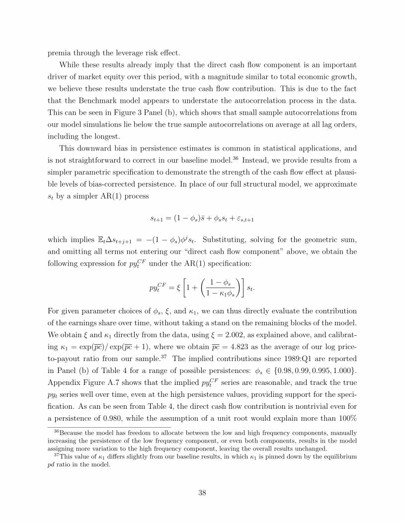
premia through the leverage risk effect.

While these results already imply that the direct cash flow component is an important

driver of market equity over this period, with a magnitude similar to total economic growth,

we believe these results understate the true cash flow contribution. This is due to the fact

that the Benchmark model appears to understate the autocorrelation process in the data.

This can be seen in Figure 3 Panel (b), which shows that small sample autocorrelations from

our model simulations lie below the true sample autocorrelations on average at all lag orders,

including the longest.

This downward bias in persistence estimates is common in statistical applications, and

is not straightforward to correct in our baseline model.36 Instead, we provide results from a

simpler parametric specification to demonstrate the strength of the cash flow effect at plausi-

ble levels of bias-corrected persistence. In place of our full structural model, we approximate

st by a simpler AR(1) process

st+1 = (1− φs)s+ φsst + εs,t+1

which implies Et∆st+j+1 = −(1 − φs)φjst. Substituting, solving for the geometric sum,

and omitting all terms not entering our “direct cash flow component” above, we obtain the

following expression for pyCFt under the AR(1) specification:

pyCFt = ξ

[1 +

(1− φs

1− κ1φs

)]st.

For given parameter choices of φs, ξ, and κ1, we can thus directly evaluate the contribution

of the earnings share over time, without taking a stand on the remaining blocks of the model.

We obtain ξ and κ1 directly from the data, using ξ = 2.002, as explained above, and calibrat-

ing κ1 = exp(pc)/ exp(pc + 1), where we obtain pc = 4.823 as the average of our log price-

to-payout ratio from our sample.37 The implied contributions since 1989:Q1 are reported

in Panel (b) of Table 4 for a range of possible persistences: φs ∈ {0.98, 0.99, 0.995, 1.000}.Appendix Figure A.7 shows that the implied pyCFt series are reasonable, and track the true

pyt series well over time, even at the high persistence values, providing support for the speci-

fication. As can be seen from Table 4, the direct cash flow contribution is nontrivial even for

a persistence of 0.980, while the assumption of a unit root would explain more than 100%

36Because the model has freedom to allocate between the low and high frequency components, manuallyincreasing the persistence of the low frequency component, or even both components, results in the modelassigning more variation to the high frequency component, leaving the overall results unchanged.

37This value of κ1 differs slightly from our baseline results, in which κ1 is pinned down by the equilibriumpd ratio in the model.

38

of the rise in the log ME/Y ratio over this period.

The question then becomes which of these persistence values is most appropriate. A

bootstrap bias corrected AR(1) estimate yields φs = 0.990 (see Appendix Section A.5.1 for

details), which corresponds to nearly half of the rise in the log ME/Y ratio being explained

through the direct influence of the earnings share on cash flows. For equity values, however,

the autocorrelation at the first lag is not as important as the autocorrelation at longer

lags. Appendix Figure A.8 reproduces the simulated autocorrelation plots from Figure 3 for

these AR(1) models, showing that even more persistent processes, such as φ = 0.995, or

even a unit root, provide a better fit of the observed longer autocorrelation pattern for st.

Although the empirical autocorrelations in the data decay substantially with the lag order,

our simulation results indicate that this is an endemic feature of sample autocorrelations

given our sample size, even for extremely persistent processes. For more formal evidence,

an augmented Dickey-Fuller test also fails to reject the presence of a unit root with p-value

0.164. From our results in Table 4, these values would imply direct cash flow contributions

of 60% or more over the 1989 - 2017 period.

Overall, this analysis implies that under minimal assumptions — that investment is

proportional to output, not earnings, and that the earnings share follows a simple AR(1)

process — the data are consistent with a strong direct effect of the earnings share on the

value of market equity over the last three decades. By contrast, the same bias correction

would have little influence on the estimated contribution of the risk-free rate, since–as shown

in Figure 3–there is no downward bias in those autocorrelations at long lag orders, which

evidently converge to zero by quarterly lag 40 in both the model and the data. We believe

these findings imply that our estimates are if anything a lower bound on the true contribution

of the earnings share to the growth in market equity since 1989.

7 Conclusion

In this paper, we investigate the causes of rising equity values over the post-war period.

We do this by estimating a flexible parametric model of how equities are priced that allows

for influence from a number of mutually uncorrelated latent components, while at the same

time inferring what values those components must have taken over our sample to explain

the data. The identification of mutually uncorrelated components and the specification of a

log linear model allow us to precisely decompose the observed market growth into distinct

component sources explaining 100% of the variation in equity values over our sample and at

each point in time.

We confront our model with data on equity values, output, the earnings share of output,

39

interest rates, and a measure of the conditional equity premium implied by options data.

We find that the high returns to holding equity over the post-war era have been attributable

in large part to an unpredictable string of factor share shocks that reallocated rewards away

from labor compensation and toward shareholders. Indeed, our estimates suggest that at

least 2.1 percentage points of the post-war average annual log equity return in excess of

a short-term interest rate is attributable to this string of reallocative shocks, rather than

to genuine compensation for bearing risk. This estimate implies that the sample mean log

excess equity return overstates the true risk premium by 43%.

Factors share shocks alone would have driven a 116% increase in the value of real per-

capita market equity since 1989, explaining 44% of actual log growth over this period. Equity

values were modestly boosted since 1989 by persistently declining interest rates and a decline

in the price of risk, which contributed 14% and 18%, respectively, to the rise in log equity

values over this period. But growth in the real value of aggregate output contributed just

25% since 1989 and just 54% over the full sample. By contrast, economic growth was

overwhelmingly important for rising equity values from 1952 to 1988, where it explained

over 100% of the market’s rise. Still, this 37 year period generated less than half the growth

in equity wealth created in the 29 years since 1989. In this sense, factor shares, far more

than economic growth, have been the preponderant measure of fundamental value in the

stock market over the last three decades.

References

Ait-Sahalia, Yacine, Jonathan A. Parker, and Motohiro Yogo, “Luxury Goods and theEquity Premium,” Journal of Finance, 2004, 59, 2959–3004.

Ang, Andrew and Monika Piazzesi, “A No-Arbitrage Vector Autoregression of Term StructureDynamics With Macroeconomic and Latent Variables,” Journal of Monetary Economics, 2003,50, 745–787.

Bansal, Ravi and Amir Yaron, “Risks for the Long-Run: A Potential Resolution of AssetPricing Puzzles,” Journal of Finance, August 2004, 59 (4), 1481–1509.

Barro, Robert J, “Rare Disasters, Asset Prices, and Welfare Costs,” American Economic Review,2009, 99 (1), 243–64.

Bekaert, Geert, Eric Engstrom, and Yuhang Xing, “Risk, Uncertainty, and Asset Prices,”Journal of Financial Economics, 2009, 91 (1), 59–82.

Bianchi, Francesco, Martin Lettau, and Sydney C. Ludvigson, “Monetary Policy and AssetValuaton,” 2016. http://www.econ.nyu.edu/user/ludvigsons/reg.pdf.

40

Campbell, John Y. and John H. Cochrane, “By Force of Habit: A Consumption-BasedExplanation of Aggregate Stock Market Behavior,” Journal of Political Economy, 1999, 107,205–251.

and Robert J. Shiller, “The Dividend-Price Ratio and Expectations of Future Dividends andDiscount Factors,” Review of Financial Studies, 1989, 1 (3), 195–228.

, Andrew W. Lo, and Craig MacKinlay, The Econometrics of Financial Markets, Princeton,NJ: Princeton University Press, 1997.

Campbell, John Y, Carolin Pflueger, and Luis M. Viceira, “Monetary policy drivers ofbond and equity risks,” Technical Report, National Bureau of Economic Research 2014.

Chen, Xiaohong, Jack Favilukis, and Sydney C. Ludvigson, “An Estimation of EconomicModels with Recursive Preferences,” Quantitative Economics, 2014, 4 (1), 39–83.

Cochrane, John H., Asset Pricing, Revised Edition, Princeton, NJ: Princeton University Press,2005.

, “Discount Rates,” Journal of Finance, forthcoming, 2011. American Finance AssociationPresidential Speech.

Constantinides, George M. and Darrell Duffie, “Asset Pricing With Heterogeneous Con-sumers,” Journal of Political Economy, 1996, 104, 219–40.

Corhay, Alexandre, Howard Kung, and Lukas Schmid, “Q: Risk, Rents, or Growth?,”Technical Report, Technical Report 2018.

Crouzet, Nicolas and Janice Eberly, “Rents and Intangible Capital: A Q+ Framework,” 2020.Unpublished manuscript, Northwestern University.

Dai, Qiang and Kenneth Singleton, “Expectation Puzzles, Time-Varying Risk Premia, andAffine Models of the Term Structure,” Journal of Financial Economics, 2002, 63, 415–441.

Danthine, Jean-Pierre and John B. Donaldson, “Labour Relations and Asset Returns,”Review of Economic Studies, January 2002, 69 (1), 41–64.

Duffie, Darrell and Rui Kan, “A yield-factor model of interest rates,” Mathematical finance,1996, 6 (4), 379–406.

Durbin, James and Siem Jan Koopman, “A simple and efficient simulation smoother for statespace time series analysis,” Biometrika, 2002, 89 (3), 603–616.

Eisfeldt, Andrea L, Antonio Falato, and Mindy Z Xiaolan, “Human capitalists,” Availableat SSRN 3375849, 2018.

Estrada, Javier, “Blinded by growth,” Journal of Applied Corporate Finance, 2012, 24 (3), 19–25.

Farhi, Emmanuel and Francois Gourio, “Accounting for Macro-Finance Trends: MarketPower, Intangibles, and Risk Premia,” Technical Report, National Bureau of Economic Research2018.

41

Favilukis, Jack and Xiaoji Lin, “The Elephant in the Room: The Impact of Labor Obligationson Credit Risk,” 2013. https://sites.google.com/site/jackfavilukis/WageCreditRisk.pdf.

and , “Wage Rigidity: A Quantitative Solution to Several Asset Pricing Puzzles,” The Reviewof Financial Studies, 2015, 29 (1), 148–192.

and , “Does wage rigidity make firms riskier? Evidence from long-horizon return predictabil-ity,” Journal of Monetary Economics, 2016, 78, 80–95.

Gelman, Andrew, Hal S Stern, John B Carlin, David B Dunson, Aki Vehtari, andDonald B Rubin, Bayesian Data Analysis, Chapman and Hall/CRC, 2013.

Gomez, Matthieu, “Asset prices and wealth inequality,” 2016. Unpublished paper: Princeton.http://www. princeton. edu/˜ mattg/files/jmp. pdf.

Greenwald, Daniel, Martin Lettau, and Sydney C. Ludvigson, “Origins of Stock MarketFluctuations,” 2014. National Bureau of Economic Research Working Paper No. 19818.

Guvenen, M. Fatih, “A Parsimonious Macroeconomic Model for Asset Pricing,” Econometrica,2009, 77 (6), 1711–1740.

Haario, Heikki, Eero Saksman, Johanna Tamminen et al., “An Adaptive Metropolis Algo-rithm,” Bernoulli, 2001, 7 (2), 223–242.

Herbst, Edward and Frank Schorfheide, “Sequential Monte Carlo Sampling for DSGE Mod-els,” Journal of Applied Econometrics, 2014, 29 (7), 1073–1098.

Jermann, Urban, “Asset Pricing in Production Economies,” Journal of Monetary Economics,April 1998, 41 (2), 257–275.

Karabarbounis, Loukas and Brent Neiman, “The Global Decline of the Labor Share,” Quar-terly Journal of Economics, October 2013, 129 (1), 61–103.

Klein, Lawrence R and Richard F Kosobud, “Some econometrics of growth: Great ratios ofeconomics,” The Quarterly Journal of Economics, 1961, 75 (2), 173–198.

Koh, Dongya, Raul Santaeulalia-Llopis, and Yu Zheng, “Labor share decline and intellectualproperty products capital,” Available at SSRN 2546974, 2016.

Lansing, Kevin J., “Asset Pricing with Concentrated Ownership of Capital and DistributionShocks,” 2014. Federal Reserve Bank of San Francisco Working Paper 2011-07.

Lansing, Kevin J, “Replicating Business Cycles and Asset Returns with Sentiment and Low RiskAversion,” 2021.

Lettau, Martin and Jessica A. Wachter, “Why is Long-Horizon Equity Less Risky? A Dura-tion Based Explanation of the Value Premium,” Journal of Finance, February 2007, LXII (1),55–92.

and Sydney C. Ludvigson, “Consumption, Aggregate Wealth and Expected Stock Returns,”Journal of Finance, June 2001, 56 (3), 815–849.

and , “Euler Equation Errors,” The Review of Economic Dynamics, 2009, 12 (2), 255–283.

42

and Sydney C Ludvigson, “Shocks and Crashes,” in Jonathan Parker and Michael Woodford,eds., National Bureau of Economics Research Macroeconomics Annual: 2013, Vol. 28, Cambridgeand London: MIT Press, 2013, pp. 293–354.

, Sydney C. Ludvigson, and Sai Ma, “The Momentum Undervalue Puzzle,” 2018. Unpub-lished paper, NYU.

, , and , “Capital Share Risk in U.S. Asset Pricing,” The Journal of Finance, 2019, 74 (4),1753–1792.

Ludvigson, Sydney C., “Advances in Consumption-Based Asset Pricing: Empirical Tests,” inGeorge Constantinides, Milton Harris, and Rene Stulz, eds., Handbook of the Economics ofFinance Vol. II, North Holland, Amsterdam: Elsevier Science B.V., 2012, pp. 799–906.

Lustig, Hanno and Stijn Van Nieuwerburgh, “The Returns on Human Capital: Good Newson Wall Street is Bad News on Main Street,” Review of Financial Studies, 2008, 21, 2097–2137.

, , and Adrien Verdelhan, “The wealth-consumption ratio,” Review of Asset Pricing Stud-ies, 2013, 3 (1), 38–94.

Malloy, Christopher J., Tobias J. Moskowitz, and Annette Vissing-Jorgensen, “Long-runStockholder Consumption Risk and Asset Returns,” Journal of Finance, 2009, 64, 2427–2479.

Mankiw, N. Gregory, “The Equity Premium and the Concentration of Aggregate Shocks,”Journal of Financial Economics, March 1986, 17, 97–112.

and Stephen P. Zeldes, “The Consumption of Stockholders and Nonstockholders,” Journalof Financial Economics, March 1991, 29 (1), 97–112.

Marfe, Roberto, “Income Insurance and the Equilibrium Term Structure of Equity,” 2016.http://robertomarfe.altervista.org/.

Martin, Ian, “What is the Expected Return on the Market?,” The Quarterly Journal of Eco-nomics, 2017, 132 (1), 367–433.

Ritter, Jay R, “Is Economic Growth Good for Investors? 1,” Journal of Applied CorporateFinance, 2012, 24 (3), 8–18.

Siegel, Jeremy J., Stocks for the Long Run: The Definitive Guide to Financial Market Returnsand Long-term Investment Strategies, 5 ed., New York, NY: McGraw Hill, 2014.

Summers, Lawrence H, “On economics and finance,” The Journal of Finance, 1985, 40 (3),633–635.

Vissing-Jorgensen, Annette, “Limited Asset Market Participation and Intertemporal Substitu-tion,” Journal of Political Economy, 2002, 110 (4), 825–853.

Wachter, Jessica, “Can Time-Varying Risk of Rare Disasters Explain Aggregate Stock MarketActivity?,” Journal of Finance, 2013, 68, 987–1035.

43

Appendix: For Online Publication

A.1 Data Description

Corporate Equity. Corporate equity is obtained from the Flow of Funds Table B103, se-

ries code LM103164103, nonfinancial corporate business; corporate equities; liability. Unad-

justed transactions estimated by Federal Reserve Board (Capital Markets and Flow of Funds

Sections), using data from the following commercial sources: cash mergers and acquisitions

data from Thompson Financial Services SDC database; public issuance and share repurchase

data from Standard and Poor’s Compustat database; and private equity issuance data from

Dow Jones Private Equity Analyst and PriceWaterhouseCoopers Money tree report. Level

at market value is obtained separately as the sum of the market value of the nonfinancial

corporate business (FOF series LM103164103) and the financial corporate business (FOF

series LM793164105). Source: Federal Reserve Board.

Foreign Earnings. Total earnings is the sum of domestic after-tax profits from NIPA

and earnings of U.S. multinational enterprises on their overseas operations. Total earnings

are defined as as share of domestic net-value-added for the corporate sector. (See the next

subsection for the sources of domestic data.)

Et = StYt

=(SDt Zt + Ft

)Yt.

In the above, Ft is the foreign profit share of domestic output. The measure of foreign

profits in the numerator of Ft is based on data from Table 4.2 of the U.S. International

Transactions in Primary Income on Direct Investment, obtained from BEA’s International

Data section. We refer to this simply as corporate “direct investment.” Specifically, these

data are from the “income on equity” row 2 of Direct investment income on assets, as-

set/liability basis. Note that U.S. direct investment abroad is ownership by a U.S. investor

of at least 10 percent of a foreign business, and so excludes household portfolio investment.

This series is available from 1982:Q1 to the present. To extend this series backward, we first

take data on net foreign receipts from abroad (Corporate profits with IVA and CCAdj from

BEA NIPA Table 1.12. (A051RC) or from Flow of Funds (FOF) Table F.3 (FA096060035.Q

less corporate profits with IVA and CCAdj, domestic industries from BEA NIPA Table 1.14

(A445RC)), which is available from the post-war period onward. This series includes port-

folio investment income of households as well as direct investment, but its share of domestic

net-value-added for the corporate sector is highly correlated with the foreign direct invest-

ment share of net-value-added. We regress the direct investment share of net-value-added on

the foreign receipts share of domestic net-value-added and then use the fitted value from this

regression as the measure of Ft in data pre-1982. Because the portfolio income component

is relatively small, the fit of this regression is high, as seen in Figure A.1, which compares

the fitted series with the actual series over the post-1982 period.

Figure A.1: Net Foreign Income Share: Data vs. Fitted value

1950 1960 1970 1980 1990 2000 2010

0.010

0.015

0.020

0.025

0.030

0.035

0.040

0.045 BEA Net Foreign Inc. ShareFitted Value

Notes: The sample spans the period 1952:Q1-2018:Q2.

Domestic Variables: Corp. Net Value Added, Corp. Labor Compensation, Corp.

After-Tax Profits, Taxes, and Interest. Define domestic corporate earnings EDt as

EDt = SDt (1− τt)NV At,

which is equivalent to

EDt =

1− LCtATPt + LCt︸ ︷︷ ︸

Labor share of labor+profit

(1− τt)NV At.

Data for the net value added (NV A) comes from NIPA Table 1.14 (corporate sector series

codes A457RC1 and A438RC1). We use per capita real net value added, deflated by the

implicit price deflator for net value added. After tax profits (ATP) for the domestic sector

come from NIPA Table 1.14 (corporate sector series code: W273RC1). Corporate sector

labor compensation (LC) for the domestic sector is from Table 1.14 (series code A442RC).

The doestic after-tax profit share (ATPS) of NV A is identically equal to

ATPS =ATP

ATP + LC

ATP + LC

NV A=

ATP

ATP + LC︸ ︷︷ ︸=SD

t

NV A− (taxes and interest)

NV A

= SDt

1−(

taxes and interest

NV A

)︸ ︷︷ ︸

=τt

= SDt Zt,

where SDt is the domestic after-tax profit share of combined profit plus labor compensation,

“taxes and interest” is the sum of taxes on production and imports less subsidies (W325RC1),

net interest and miscellaneous payments (B471RC1), business current transfer payments

(Net) (W327RC1), and taxes on corporate income (B465RC1). Source: Bureau of Economic

Analysis.

Net Dividends Plus Net Repurchases (Equity Payout). Net dividends minus net

equity issuance is computed using flow of funds data. Net dividends (“netdiv”) is the se-

ries named for corporate business; net dividends paid (FA096121073.Q). Net repurchases

are repurchases net of share issuance, so net repurchases is the negative of net equity is-

suance. Net equity issuance (“netequi”) is the sum of Equity Issuance for Nonfinancial

corporate business; corporate equities; liability (Table F.103, series FA103164103) and Eq-

uity Issuance for domestic financial sectors; corporate equities; liability (Table F.108, series

FA793164105). Since netdiv and netequi are annualized, the quarterly payout is computed

as payout=(netdiv-netequi)/4. The units are in millions of dollars. Source: Federal Reserve

Board.

Price Deflators. Implicit price deflator and GDP deflator. A chain-type price deflator

for the nonfinancial corporate sector (NFCS) is obtained implicitly by dividing the net value

added of nonfinancial corporate business by the chained real dollar net value added of non-

financial corporate business from NIPA Table 1.14. This index is used to deflate net value

added of the corporate sector. There is no implicit price deflator available for the whole

corporate sector, so we use deflator for the non-financial corporate sector instead. The GDP

deflator is used to construct a real returns and a real interest (see below). GDPDEF is

retrieved from FRED. Our source is the Bureau of Economic Analysis.

Interest Rate. The nominal risk-free rate is measured by the 3-Month Treasury Bill rate,

secondary market rate. We take the (average) quarterly 3-Month Treasury bill from FRED

(code: TB3MS). A real rate is constructed by subtracting the fitted value from a regression

of GDP deflator inflation onto lags of inflation from the nominal rate. Our source is the

board of governors of the Federal Reserve System and the Bureau of Economic Analysis.

Risk Premium Measure. Our measure of the risk premium comes from Martin (2017).

This paper uses option data to compute a lower bound on the equity risk premium, then

argues that this lower bound is in fact tight, and a good measure of the true risk premium on

the stock market. We obtain this series from the spreadsheet epbound.xls on Ian Martin’s

website, which corresponds to the value

EPBoundt→T = 100×(Rf,tSV IX

2t→T − 1

)which is equivalent to the bound on the annualized net risk premium, in percent. To trans-

late these measures to our model’s quarterly frequency, we use the risk premium measure

computed over the next three months. We then convert this variable into a log return,

average it over the quarter, and label it rpt.

Survey Data on Expected Average Risk-Free Rate For the average short-term ex-

pected nominal interest rate, we use the mean forecast from the Survey of Professional

Forecasters for variable BILL10, which is the 10-year annual-average forecast for returns on

3-month Treasury bills. We subtract from this the mean forecast for variable CPI10, the

10-year annual-average forecast of inflation, to obtain a survey forecast for the average real

rate over the next ten years.

A.2 A Stylized Model of Workers and Shareholders

We consider a stylized limited participation endowment economy in which wealth is con-

centrated in the hands of a few asset owners, or “shareholders,” while most households are

“workers” who finance consumption out of wages and salaries. The economy is closed. Work-

ers own no risky asset shares and consume their labor earnings. There is no risk-sharing

between workers and shareholders. A representative firm issues no new shares and buys back

no shares. Cash flows are equal to output minus a wage bill,

Ct = Yt − wtNt,

where wt equals the wage and Nt is aggregate labor supply. The wage bill is equal to Yt

times a time-varying labor share αt,

wtNt = αtYt =⇒ Ct = (1− αt)Yt. (A.1)

We rule out short sales in the risky asset:

θit ≥ 0.

Asset owners not only purchase shares in the risky security, but also trade with one another in

a one-period bond with price at time t denoted by qt. The real quantity of bonds is denoted

Bt+1, where Bt+1 < 0 represents a borrowing position. The bond is in zero net supply

among asset owners. Asset owners could have idiosyncratic investment income ζ it , which is

idependently and identically distributed across investors and time. The gross financial assets

of investor i at time t are given by

Ait = θit (Vt + Ct) +Bit.

The budget constraint for the ith investor is

Cit +Bi

t+1qt + θit+1Vt = Ait + ζ it (A.2)

= θit (Vt + Ct) +Bit + ζ it ,

where Cit denotes the consumption of investor i.

A large number of identical nonrich workers, denoted by w, receive labor income and

do not participate in asset markets. The budget constraint for the representative worker is

therefore

Cw = αtYt. (A.3)

Equity market clearing requires ∑i

θit = 1.

Bond market clearing requires ∑i

Bit = 0.

Aggregating (A.2) and (A.3) and imposing both market clearing and (A.1) implies that

aggregate (worker plus shareholder) consumption CAggt is equal to total output Yt. Aggre-

gating over the budget constraint of shareholders shows that their consumption is equal to

the capital share times aggregate consumption CAggt :

CSt = Ct = (1− αt)︸ ︷︷ ︸

KSt

CAGGt .

A representative shareholder who owns the entire corporate sector will therefore have con-

sumption equal to CAggt ·KSt. This reasoning goes through as an approximation if workers

own a small fraction of the corporate sector even if there is some risk-sharing in the form of

risk-free borrowing and lending between workers and shareholders, as long as any risk-sharing

across these groups is imperfect. While individual shareholders can smooth out transitory

fluctuations in income by buying and selling assets, shareholders as a whole are less able to

do so since purchases and sales of any asset must net to zero across all asset owners.

A.3 Model Solution

Perturbation Details. The derivation of the perturbed stochastic discount factor (11)

follows here. We seek a perturbation of the terms determining the risk exposure of the SDF,

the nonlinear expression mt+1 = −xt∆ct+1. Our perturbation includes terms linear in both

the state vector zt, the shock vector εt+1, and interactions between the two, while omitting

all other higher-order terms. While our solution could handle terms quadratic in zt, they

would be irrelevant since the term µt would implicitly offset them in all states. On the other

hand, terms quadratic in εt+1 would influence the solution, but would break our solution

methodology.

To derive the perturbed stochastic discount factor, we first express mt in terms of the

current period’s states and next period’s shocks:

mt+1 = −xt{

log[exp(s+ 1′ (Φsst + εs,t+1)

)− ω

]− log

[exp(s+ 1′st

)− ω

]+ g + εy,t+1

}.

Evaluating the derivatives of this expression with respect to shocks and states, we obtain

∂mt+1

∂xt= −∆ct+11

′

∂mt+1

∂st= −xt

{(St+1

St+1 − ω

)1′Φ−

(St

St − ω

)1′}

∂mt+1

∂εs,t+1

= −xt(

St+1

St+1 − ω

)1′

∂mt+1

∂εy,t+1

= −xt

∂2mt+1

∂εs,t+1∂xt= −1

(St+1

St+1 − ω

)1′

∂2mt+1

∂εs,t+1∂st= xt1

(St+1

St+1 − ω

)(ω

St+1 − ω

)1′Φs

We therefore approximate

mt+1 ' −xg − g1′xt − xξ1′(Φs − I)st − xξ1′εs,t+1 − xεy,t+1

− x′t1ξ1′εs,t+1 + s′tΦ

′sxξ(ξ − 1)1′εs,t+1 − x′t1εy,t+1

= · · · −(xtξ − xξ(ξ − 1)(1′Φsst)

)1′εs,t+1 − xtεy,t+1

where the omitted terms are known at time t, and whose exact values are thus irrelevant

to our solution as they will be directly offset by the implicitly defined µt. Combining this

result with the identity

Et[st+1] = s+ 1′Φsst

and rearranging yields (11).

Price-Payout Ratio This section derives the coefficients of the main asset pricing equa-

tion (13). To begin, define for convenience the variables

ut+1 = log(PCt+1 + 1)− pctqt+1 = mt+1 + ∆ct+1

so that mt+1 + rt+1 = ut+1 + qt+1. Applying the log linear approximation to log(PCt+1 + 1)

and substituting in our guessed functional form (13) yields

ut+1 = log(PCt+1 + 1)− pdt

= κ0 + κ1

(A0 + A′sst+1 + A′xxt+1 + A′δδt

)−(A0 + A′sst + A′xxt + A′δδt

)= κ0 + (κ1 − 1)A0 + A′s (κ1Φs − I) st + A′x(κ1Φx − I)xt + A′δ(κ1Φδ − I)δt

+ κ1A′sεs,t+1 + κ1A

′xεx,t+1 + κ1A

′δεδ,t+1.

Now turning to qt+1, we can expand the expression to yield

qt+1 = −δt − µt + g + ξEt∆st+1 + (1− γs,t)ξ1′εs,t+1 + (1− xt)εy,t+1

where

γs,t = xt − x(1− ξ)(Et[st+1]− s)

= x+ 1′xt − x(1− ξ)1′Φst

= x+ 1′xt + Γ′st.

for

Γ′ = −x(1− ξ)1′Φs.

Next, we apply our fundamental asset pricing equation 0 = logEt [qt+1 + ut+1], which under

lognormality implies

0 = Et[qt+1] + Et[ut+1] +1

2Vart(qt+1) +

1

2Vart(ut+1) + Cov(qt+1, ut+1).

These moments can be calculated as

Et[qt+1] = −δt − µt + g − ξ1′(I−Φs)st

Et[zt+1] = κ0 + (κ1 − 1)A0 + A′s (κ1Φs − I) st + A′x(κ1Φx − I)xt + A′δ(κ1Φδ − I)δt

Vart(qt+1) = (1− γs,t)2ξ2(1′Σs1) + (1− xt)2σ2a

Vart(zt+1) = κ21

(A′sΣsA

′s + A′xΣxAx + A′δΣrAδ

)Covt(qt+1, zt+1) = κ1ξ(1− γs,t)A′sΣs1

Substituting, we obtain

0 = −δ + g + κ0 + (κ1 − 1)A0 +1

2

((1− 2x)ξ2(1′Σs1) + (1− 2x)σ2

a

)+

1

2κ2

1

(A′sΣsA

′s + A′xΣxAx + A′δΣrAδ

)+ κ1ξ(1− x)A′sΣs1

+[−ξ1′(I−Φs) + A′s (κ1Φs − I)− ξ2(1′Σs1)Γ′s − κ1ξΓ

′sA′sΣs1

]st

+[A′x(κ1Φx − I)− ξ2(1′Σs1)1′ − 1′σ2

a − κ1ξ1′A′sΣs1

]xt

+[A′δ(κ1Φδ − I)− 1

]δt.

Applying the method of undetermined coefficients now yields the solutions

A′s =[ξ1′(I−Φs)− ξ2(1′Σs1)Γ′s

][(κ1Φs − I) + κ1ξΣs1Γ′s

]−1

A′x =[(ξ2(1′Σs1) + σ2

a + κ1ξ(A′sΣs1)

)1′](κ1Φx − I)−1

A′δ = 1(κ1Φδ − I)−1

while the constant term must solve

0 = −δ + g + κ0 + (κ1 − 1)A0 +1

2

((1− 2x)ξ2(1′Σs1) + (1− 2x)σ2

a

)+

1

2κ2

1

(A′sΣsA

′s + A′xΣxAx + A′δΣrAδ

)+ κ1ξ(1− x)A′sΣs1.

(A.4)

A.3.1 Equilibrium Selection

The parameters κ0 and κ1 determine the steady state pc (price-payout ratio), which depends

on A0. But since κ0 and κ1 are both themselves nonlinear functions of A0, the equilibrium

condition (A.4) is also nonlinear, leading to the possibility that multiple solutions, or no

solution, exists. In fact, we confirm that both of these outcomes can occur in our numerical

solutions. However, our numerical results indicate that, when there is more than one solution

there are at most two, and one can be discarded because it is economically implausible. To

see this, rewrite (A.4) as

0 = E[m] + E[r] +1

2Var(m) +

1

2Var(r) + Cov(m, r)

where m and r are the log SDF and equity return. We are interested in the relationship

between the steady state pc and the other terms that depend on it in equilibrium. The terms

E[m] and Var(m) do not depend on the pc ratio, so we can ignore these and focus on the

remaining terms. Alternatively, consider the log risk premium, given in equilibrium by

E[rt+1]− rf,t = −1

2Var(rt+1)− Cov(mt+1, rt+1).

In the case where there are two solutions, one solution typically has a plausible level for the

steady state pc, and implies that higher pc ratios (which take different values depending on

where in the posterior distribution of model parameters we evaluate the function) coincide

with lower risk premia E[rt+1] − rf,t and a lower absolute covariance with the SDF (i.e., a

less negative Cov(mt+1, rt+1)). This solution is economically reasonable. By contrast, when

there is a second solution, it is always characterized by values for pc that are higher than the

economically reasonable solution, and for typical parameter values delivers a value for pc that

are extremely implausible (e.g., a value for exp (pc) of almost 3,000 at the posterior mode).

In addition, this solution has the property that the higher pc ratios coincide with lower

risk premia vis-a-vis the plausible solution, but also higher absolute covariances with the

SDF (i.e., a more negative Cov(mt+1, rt+1)). Thus the higher pc ratios in this solution must

be explained by a lower absolute covariance with the SDF and a Jensen’s term 12Var(rt+1)

that in some cases converges to infinity. In summary, since the higher pc solution typically

implies extreme values and unreasonable behavior of pc, we select between these solutions

by enforcing that the equilibrium chosen always chooses the lower pc solution.

A.3.2 Expected Returns

Combining the relations

0 = logEt[Mt+1Rt+1]

= Et[mt+1] + Et[rt+1] +1

2Vart(mt+1) +

1

2Vart(rt+1) + Covt(mt+1, rt+1)

−rf,t = logEt[Mt+1]

= Et[mt+1] +1

2Vart(mt+1)

and rearranging, we obtain

logEt[Rt+1/Rf,t] = Et[rt+1] +1

2Vart(rt+1)− rf,t

= −Covt(mt+1, rt+1).

Since

rt+1 = constt + κ1

(A′sεs,t+1 + A′xεx,t+1 + Aδεδ,t+1

)︸ ︷︷ ︸

pc growth

+ ξ1′εs,t+1 + εa,t+1︸ ︷︷ ︸cash flow growth

mt+1 = constt − γs,t1′εs,t+1 − xtεa,t+1

we obtain

Covt(mt+1, rt+1) = −γs,t(κ1A

′s + ξ1′

)Σs1− xtσ2

a

Substituting for γs,t and rearranging yields (14).

A.3.3 Forecasting Real Rates

This section derives our 40Q average real rate forecast in the model. As an intermediate

step, note that for a given matrix A, the geometric sum, assuming it converges, is equal to

∞∑j=0

Aj = I + A∞∑j=0

Aj

which implies∞∑j=0

Aj = (I − A)−1.

Similarly the partial sum can be obtained as

N−1∑j=0

Aj =∞∑j=0

Aj −∞∑j=N

Aj =∞∑j=0

Aj − AN(∞∑j=0

Aj

)= (I − A)−1 − (I − A)−1AN

= (I − A)−1(I − AN).

Applying this to our interest rate forecast, we have

rNf,t =1

N

N−1∑j=0

Etδt+j = δ +1

N1′

N−1∑j=0

Etδt+j.

Since our law of motion for δ implies Etδt+j = Φjδδt, we can substitute to obtain

rNf,t = δ +1

N1′

(N−1∑j=0

Φjδ

)δt

= δ +1

N1′(I −Φδ)

−1(I −ΦNδ )δt

where the last line follows from our partial geometric sum formula above.

A.3.4 Bond Pricing

We can represent our model in the form

logMt+1 = −δt −1

2Λ′tΣΛt − Λ′tεt+1

where

Λt = Λ0 + Λ1zt

=

ξx

0

0

x

︸ ︷︷ ︸

Λ0

+

−xξ(ξ − 1)1′Φs ξ1′ 0 0

0 0 0 0

0 0 0 0

0 1′ 0 0

︸ ︷︷ ︸

Λ1

st

xt

δt

∆at

︸ ︷︷ ︸

zt

.

To price a zero-coupon bond of maturity n, we guess that the log bond price pn,t takes the

functional form

pn,t = An +B′nzt.

This guess is trivially verified for n = 0, with p0,t = 0 implying the initialization A0 = 0,

B′0 = 0. To prove by induction, assume the claim holds for n. Then we have

pn+1,t = logEt exp

{−δt −

1

2Λ′tΣΛt − Λ′tεt+1 + An +B′nΦzzt +B′nεt+1

}= logEt exp

{−δt −

1

2Λ′tΣΛt + (B′n − Λ′t)εt+1 + An +B′nΦzzt

}= logEt exp

{−δ0 − δ′1zt −

1

2Λ′tΣΛt + (B′n − Λ′t)εt+1 + An +B′nΦzzt

}= −δ0 − δ′1zt −

1

2Λ′tΣΛt +

1

2B′nΣBn −B′nΣΛt +

1

2Λ′tΣΛt + An +B′nΦzzt

= −δ0 − δ′1zt +1

2B′nΣBn −B′nΣΛ0 −B′nΣΛ1zt + An +B′nΦzzt

=

(−δ0 +

1

2B′nΣBn −B′nΣΛ0 + An

)+ (−δ′1 −B′nΣΛ1 +B′nΦz) zt

which implies

An+1 = −δ0 +1

2B′nΣBn −B′nΣΛ0 + An

B′n+1 = −δ′1 −B′nΣΛ1 +B′nΦz.

This both completes the proof and provides the recursion used to compute long-term real

bond prices in our model.

A.4 Estimation Details

This section provides additional details on our state space specification and estimation pro-

cedure.

Measurement Equation. To construct measurement equation, we relate our observed

series to the model’s primitive parameters and latent state variables using the following

system of equations:

eyt = 1′st

rf,t = 1′δt

r40f,t =

1

40

40−1∑j=0

Etδt+j = δ +1

401′(I −Φδ)

−1(I −Φ40δ )δt + ν

pyt = pct + cyt

= py + (A′s + ξ′) st + A′δδt + A′xxt

∆yt = g + ∆at

rpt =(Ψ + σ2

a

)(x+ 1′xt)−ΨΓ′st.

where cyt = ct − yt, and py = A0 + c + ξ′s.38 For the real risk-free rate forecast (r40f,t), the

parameter ν allows for an average difference between the model and data forecasts due to

the different inflation series used (CPI for the forecasts vs. the GDP deflator for the model),

as well as any average bias among the forecasts.39

Time Variation in State Space. To begin, we provide additional details on time varia-

tion in our state space measurement equation (15). Because our risk premium measure rpt

is not available over the full sample, we use a time varying measurement equation to accom-

modate the missing values. In periods when our measure of the risk premium is available

(1996:Q1 to 2012:Q1), equation (15) takes the form

eyt

rft

r40f,t

pyt

∆yt

rpt

=

[H1

H2

]zt +

[b1

b2

]

where H2 and b2 are the rows of the measurement matrix and constant vector that compute

the implied value for rpt, and H1 and b1 are the respective values for the other observables.

38We note that ∆at is exactly pinned down by the observation equation for ∆yt.39A full derivation of the formula for r40f,t can be found in Appendix A.3.3.

In periods when data on rpt is not available, equation (15) instead takes the formeyt

rft

r40f,t

pyt

∆yt

= H1zt + b1.

A completely analogous procedure is used for the SPF forecast variable r40f,t, since these

forecasts are also not available over the entire sample. During periods when the forecast

data are available, we expand the measurement equation (15) to include an additional row,

while for periods when the data are not available, we omit this row.

MCMC Details. We next describe the procedure used to obtain the parameter draws.

First, because some of our variables are bounded by definition (e.g., volatilities cannot be

negative), we define a set of parameter vectors satisfying these bounds denoted Θ. We

exclude parameters outside of this set, which formally means that we apply a Bayesian prior

p(θ) =

const for θ ∈ Θ

0 for θ /∈ Θ

Our restrictions on Θ are as follows: all volatilities (σ) and the average risk price x are

bounded below at zero. All persistence parameters (φ) are bounded between zero and unity.

With these bounds set, we can evaluate the posterior by

π(θ) = L(y|θ)p(θ).

so that the posterior is simply proportional to the likelihood over Θ and is equal to zero

outside of Θ.

To draw from this posterior, we use a Random Walk Metropolis Hastings algorithm. We

initialize the first draw θ0 at the mode, and then iterate on the following algorithm:

1. Given θj, draw a proposal θ∗ from the distribution N (θj, cΣθ) for some scalar c and

matrix Σθ defined below.

2. Compute the ratio

α =π(θ∗)

π(θj).

3. Draw u from a Uniform [0, 1] distribution.

4. If u < α, we accept the proposed draw and set θj+1 = θ∗. Otherwise, we reject the

draw and set θj+1 = θj.

For the covariance term, we initialize Σθ to be the inverse Hessian of the log likelihood

function at the mode. Once we have saved 10,000 draws, we begin updating Σθ to be the

sample covariance of the draws to date, following Haario, Saksman, Tamminen et al. (2001),

with the matrix re-computed after every 1,000 saved draws. For the scaling parameter c,

we initialize it at 2.4/length(θ) as recommended in Gelman, Stern, Carlin, Dunson, Vehtari

and Rubin (2013). To target an acceptance rate for our algorithm of 25%, we adapt the

approach of Herbst and Schorfheide (2014) in updating

cnew = cold ·(

0.95 + 0.1exp(16(x− 0.25))

1 + exp(16(x− 0.25))

)after every 1,000 saved draws, where cold is the pre-update value of c.

With these methods in place, we compute our estimation results in ten independent

chains, each containing 550,000 draws of θ. We discard the first 50,000 draws from each

chain as burn-in, leaving 5,000,000 parameter draws. Since these draws are highly serially

correlated, we increase computational efficiency in most applications by using every 500th

draw, leaving a total of 10,000 draws over which our margins of parameter uncertainty are

computed.

A.5 Additional Details

A.5.1 Bootstrap Bias Correction

The bootstrap bias corrected estimate for the AR(1) model of the log earnings share is

computed as follows. First, we run the regression

st = a+ φst−1 + εs,t (A.5)

to obtain the estimates aOLS, φOLS. We then bootstrapping many samples from the data

generating process

sjt = aOLS + φOLS + εjs,t

where residuals εjs,t are drawn with replacement from {εs,t}. For each j in 100,000 simulations,

we repeat the regression (A.5) to obtain estimates aj, φj, which we average to obtain the

estimates aboot, φboot. The approximate bias is computed as φOLS − φboot, implying that the

corrected persistence estimator is obtained as

φ∗ = φOLS +(φOLS − φboot

).

A.6 Model-Implied Cash Flows

This section compares implied cash flows in the model to actual cash flows in the data.

Because our model obtains implied cash flows from earnings, using (3), or its log-linear

approximation (10), rather than using actual payout data, it is important to check that

these series are sufficiently close.

Figure A.2 displays the model-implied cash flow share of output against the actual payout

share from the data. The figure shows that the series line up moderately well, particularly

toward the end of the sample, and that the model-implied series is able to reproduce a large

rise in payouts over the second half of the sample. At the same time, the two series display

nontrivial discrepancies at higher frequences.

Figure A.2: Cash Flow Share, Implied vs. Data

1960 1970 1980 1990 2000 2010

0.05

0.00

0.05

0.10

0.15

Payout Share (True)Payout Share (Approx)

Notes: This figure compares the implied cash flow series used by our model Ct = (St − ω)Et, compared tothe true corporate payout series in the data. The implied series takes St and Et directly from the data, anduses the calibrated value ω = 0.0601 consistent without our calibration of ξ.

In our model, low frequency variation in cash flows are ultimately much more important

for asset valuation. To focus in on the lower-frequency trend in cash flows, we split our

payout data into its two component series: net dividends, and net repurchases (i.e., the

negative of net equity issuance), displayed in Figure A.3. Figure A.3a display the raw series,

showing that the net dividend share is always positive and exhibits slow and persistent

dynamics, while the net repurchase share is close to zero on average and fluctuates wildly

at high frequencies. Although repurchases have become an increasingly important form of

payout, they largely cancel out with issuance of new equity, yielding a series without a major

discernible trend. As a result, Panel (b) shows that we can effectively treat the net dividend

share as a good measure of the low frequency trend in payouts, with the exception of the

transitory downward spike in net dividends during the financial crisis.

Figure A.3: Payout Data Components

(a) Net Dividend vs. Net Repurchase Shares

1960 1970 1980 1990 2000 2010

0.15

0.10

0.05

0.00

0.05

0.10Net Dividend ShareNet Repurchase Share

(b) Payout Share vs. Net Dividend Share

1960 1970 1980 1990 2000 2010

0.05

0.00

0.05

0.10

0.15

Payout ShareNet Dividend Share

Notes: Panel (a) separately displays the two components of total payout: the net dividend share (equalto (net dividends) / (net value added) for the corporate sector) and the net repurchase share ((−1)× (netequity issuance) / (net value added) for the corporate sector). Panel (b) compares the net dividend shareas just defined to the payout share (payouts / (net value added) for the corporate sector, where payouts arenet dividends minus net equity issuance). Source: Flow of Funds.

With the net dividend share as a proxy for the low frequency trend in the payout share

in the data, we can compare it to its counterpart in the model. This can be computed using

(10) as

cyLF,t = cy + ξsLF,t. (A.6)

The resulting series is displayed alongside the net dividend share in Figure A.4. Unlike the

implied series for cyt in Figure A.2, which can be computed directly from the data given ξ,

computing cyLF,t depends on the decomposition of the earnings share into its low and high

frequency components, and therefore on the model’s parameter and latent state estimates.

This leads to uncertainty in our estimate, characterized by the blue error bands, while the

median is plotted in red.

Figure A.4 shows that the model’s implied low frequency component cash flows delivers

an excellent fit of the net dividend share in the data. The fit is particularly good over the

Figure A.4: Low Frequency Cash Flow Share, Model vs. Data

1950 1960 1970 1980 1990 2000 2010 2020

0.04

0.06

0.08

0.10

0.12Net Dividend Share (Data)Implied LF Cash Flow Share (Model)

Notes: Net Dividend Share is the ratio of net dividends to net value added for the corporate sector (source:Flow of Funds). Implied LF Cash Flow Share is equal to cyLF,t in equation (A.6). The red line represents themedian outcome over our estimates, while the dark and light blue bands represent 66.7% and 90% confidenceintervals, respectively.

subsample since 1989 on which our main results are based, and does not overstate the growth

in payouts. The main discrepancy between the series is the transitory downward spike in

the data during the financial crisis, which is not really representative of the low frequency

trend, and in fact was more severe in the net dividends data than in the overall payout data,

likely due to a slowdown in equity issuance at this time.

In summary, these results provide strong support for our model’s approximate cash flow

series (10). Although the implied and data series differ at high frequencies, these discrepan-

cies largely reflect the timing of payouts, and should not play a huge role in equity pricing.

At the same time, the model is highly effective at capturing the underlying trend in payouts

through its low frequency component, providing an excellent fit for the data.

A.7 Model-Implied Real Bond Rates

In this section, we compare the implied rates on long real bonds (TIPS) in the model and

data. Figure A.5 displays 10-year real bond yields in the model alongside 10-year TIPS

yields in the data (details on this computation can be found in Appendix A.3.4). To allow

for the fact that TIPS are computed using CPI inflation while our real rates are computed

using the GDP deflator, as well as for the possibility that 10-year TIPS may include term

or liquidity premia on average, we add a constant to our model-implied TIPS rate, equal

to 0.61%, so that our model-implied and actual TIPS rates have the same mean over the

subsample over which TIPS data are available (2003:Q1 - 2017:Q4). Panel (a) displays the

full sample, while Panel (b) zooms in on the 2003:Q1 - 2017:Q4 TIPS subsample.

Figure A.5: 10-Year TIPS Yields, Model vs. Data

(a) Full Sample

1960 1970 1980 1990 2000 20101

0

1

2

3

4

10Y TIPS (Data)10Y TIPS (Model)

(b) TIPS Sample

2004 2006 2008 2010 2012 2014 2016

0.5

0.0

0.5

1.0

1.5

2.0

2.5

10Y TIPS (Data)10Y TIPS (Model)

Notes: These plots compare the yields on ten-year real bonds in model and data. The data measure isobtained from the Federal Reserve Board of Governors (FRED code: FII10). The model value is obtainedusing the bond pricing formulas in Appendix A.3.4. The red line displays the mean estimate taken over 10,000equally spaced parameter draws, while the light and dark blue bands represent 67% and 90% confidenceintervals, respectively. The left panel displays the full sample period 1952:Q1-2017:Q4, while the right paneldisplays the 2003:Q1-2017:Q4 subsample on which the TIPS data is available.

Comparing the series in Figure A.5 shows that the general trajectory of the model-implied

TIPS yields closely matches the data. Model and data yields display similar overall declines

over the sample, equal to 1.22% and 1.55% from 2003:Q1 (the start of the TIPS sample)

to 2017:Q3, respectively. Similarly, model and data yields exhibit falls of 1.65% and 1.85%

from the 2006:Q3 (the TIPS peak, outside of a brief spike during the financial crisis) to

2017:Q4, respectively. Although Panel (b) shows some deviations between model and data

— in particular a failure of the model to capture a dip in rates between 2012 and 2013 —

these results show that the model explains most movements in real long-term bonds at the

10-year horizon, despite the fact that these data are not a target of the estimation.

A.8 Additional Figures

Figure A.6: Model-Implied Risk-Free Rate Forecast

1960 1970 1980 1990 2000 2010

0.00

0.01

0.02

0.03

0.0410-Year Real Rate ForecastModel Estimate

Figure A.7: Implied Contributions, AR(1) Models

(a) Full Sample

1960 1970 1980 1990 2000 2010

0.50

0.25

0.00

0.25

0.50

0.75

1.00

1.25Data

s = 1.000s = 0.995s = 0.990s = 0.980

(b) Since 1989

1992 1996 2000 2004 2008 2012 2016

0.00

0.25

0.50

0.75

1.00

1.25

1.50

1.75Data

s = 1.000s = 0.995s = 0.990s = 0.980

Notes: This figure superimposes the implied contributions of the earnings share to the log market equityto output ratio via cash flows measured as in equation (16), over the earnings share data. Each impliedcontribution is computed by adding the difference in the right hand side of (16) to the initial value of pyt atthe start of the relevant subsample.

Figure A.8: Simulated Autocorrelations, AR(1) Models

(a) φs = 0.98

0 5 10 15 20 25 30 35 40

0.2

0.0

0.2

0.4

0.6

0.8

1.0

(b) φs = 0.99

0 5 10 15 20 25 30 35 40

0.2

0.0

0.2

0.4

0.6

0.8

1.0

(c) φs = 0.995

0 5 10 15 20 25 30 35 400.2

0.0

0.2

0.4

0.6

0.8

1.0

(d) φs = 1

0 5 10 15 20 25 30 35 400.2

0.0

0.2

0.4

0.6

0.8

1.0

Notes: The figure compares the data autocorrelations for the observable variables available over the fullsample, compared to the same statistics from the simplified AR(1) models described in Section 6. For themodel equivalents, we compute autocorrelations from each of 10,000 simulations the same length as thedata, drawn with the persistence parameter found in that panel’s title. The center line corresponds to themean of these autocorrelations, while the dark and light gray bands represent 66.7% and 90% credible sets,respectively. The sample spans the period 1952:Q1-2017:Q4.