how to feed the world in 2050: macroeconomic environment

Munich Personal RePEc Archive

How to feed the world in 2050:

Macroeconomic environment, commodity

markets - A longer term outlook

van der Mensbrugghe, Dominique and Osorio Rodarte, Israel

and Burns, Andrew and Baffes, John

The World Bank, FAO

12 October 2009

Online at https://mpra.ub.uni-muenchen.de/19061/

MPRA Paper No. 19061, posted 08 Dec 2009 07:45 UTC

Expert Meeting on How to feed the World in 2050

Food and Agriculture Organization of the United Nations

Economic and Social Development Department

* The World Bank, 1818 H Street, NW, Washington, D.C. 20433, United States of America.

Paper prepared for the Expert Meeting on How to feed the World in 2050, FAO Headquarters, Rome, 24-26 June 2009. The views expressed in this information product are those of the author(s) and do not necessarily reflect the views of the Food and Agriculture Organization of the United Nations.

MACROECONOMIC ENVIRONMENT, COMMODITY MARKETS: A LONGER TERM OUTLOOK

Dominique van der Mensbrugghe, Israel Osorio-Rodarte, Andrew Burns and John Baffes*

ABSTRACT

The recent commodity boom was the longest and broadest of the post-World War II period. Although most prices have declined sharply since their mid-2008 peak, they are still considerably higher than 2003, the beginning of the boom. Apart from strong and sustained economic growth, the recent boom was fueled by numerous other factors including low past investment in extractive commodities, weak dollar, fiscal expansion in many countries, and, perhaps, investment fund activity. On the other hand, the diversion of some food commodities to the production of biofuels, adverse weather conditions, global stock declines to historical lows and government policies, including export bans and prohibitive taxes, accelerated the price increases that eventually led to the 2008 rally. This paper concludes that the increased link between energy and non-energy commodity prices, strong demand by developing countries - when the current economic downturn reverses course - and changing weather patterns will be the dominant forces that are likely to shape developments in commodity markets.

I. INTRODUCTION

By most accounts, the recent commodity boom was the longest and broadest (in terms of commodities involved) of the post-World War II period (World Bank 2009). Between 2003 and 2008, nominal energy and metal prices increased by 230 percent, food and precious metals doubled, while fertilizer prices increased four-fold. Although most prices have declined sharply since their mid-2008 peak, they are still considerably higher than their 2003 levels.

Apart from broad and sustained economic growth, the boom was fueled by a host of other factors both macro and long-term as well as sector-specific and short-term. These include: low past investment in extractive commodities, a reflection of a prolonged period of declining prices due excess capacity left after the collapse of the Soviet Union and weak demand after the 1997 East Asian (and other countries) financial crisis; weak dollar (the currency of choice in most international commodity transactions); fiscal expansion and loose monetary policies in many countries; investment fund activity by financial institutions which chose to include commodities in their portfolios. On the other hand, the diversion of some food commodities to the production of biofuels (notably maize in the US and edible oils in Europe), adverse weather conditions (e.g. three droughts in Australia during 2001-2007), global stock declines of several agricultural commodities to historical lows, and government policies such as export bans and prohibitive taxes further contributed to the 2008 rally. Geopolitical concerns played a key role as well, especially in energy markets.

In some sense, the above factors created the “perfect storm” which reached its zenith in July 2008 when crude oil prices averaged $133 per barrel (up 94 percent from a year earlier) and rice prices doubled within just five months (from $375 per ton in January to $757 per ton in June 2008). Not surprisingly, the weakening and/or reversal of these factors coupled with the financial crisis that erupted in September 2008 and the subsequent global economic downturn, induced sharp price declines across most commodity sectors.

2 FAO Expert Meeting on How to feed the World in 2050

24-26 June 2009

The recent boom, and especially the 2008 rally, has generated renewed interest for the determinants of commodity prices, including the role of commodity-specific factors, macroeconomic fundamentals, as well as questions on whether a permanent shift in price trends has taken place. On the other hand, food availability and food security concerns generated calls for coordinated policy actions at national (and perhaps international) level, reminiscent to actions taken in earlier booms. With that context in mind, this paper identifies and analyzes the dominant forces that are likely to shape long term developments in commodity markets. Such forces include (but they are not limited to) the increased interdependence between energy and non-energy markets, the growth prospects especially in developing countries where most consumption growth is expected to take place, the effect of climate change in the production and trade of commodities, and, at the outset, what all this implies for poverty.

The rest of the paper begins with a brief discussion recent price trends, including the causes of the recent commodity price boom. This is followed by an analysis of the energy/non-energy price link. The subsequent three sections deal with the issues of the growth prospects, global warming, and their implication on poverty. The last section concludes with a summary and a policy discussion.

II. THE NATURE OF THE RECENT COMMODITY BOOM

The recent commodity boom shares a number of similarities with earlier booms but it also has some differences. It involved almost all commodities (see figures 2.1 and 2.2) as opposed to earlier booms which involved only agriculture (Korean war) or agriculture and energy (1970s energy crisis). It was not associated with high inflation as opposed to the 1970s which was associated with inflationary pressures. On the other hand, all three booms took place against the backdrop of high and sustained economic growth. Furthermore, all three booms generated discussion on coordinated policy actions due to concerns over food security and energy availability issues.

The reasons behind the recent boom are numerous, and as many analysts have argued, they created a “perfect storm.” On the one hand, most countries enjoyed sustained economic growth for a long period of time. During 2003-07, growth in developing countries averaged 6.9 percent, the highest 5-year average in recent history (the second highest 5-year average, 6.5 percent, took place during 1969-73). Fiscal expansion in many countries and low interest rates created an environment which favored high commodity prices. The depreciation of the US dollar played some role since it is the currency of choice for most international transactions.

On extractive sectors, especially energy commodities, underinvestment during the late 1980s and 1990s left limited room for supply response. For example, during the early 1980s, total investment expenditures by the major US multinational oil and gas companies averaged more than $130 billion annually (real 2006 terms). For the next 15 years, however, the annual average dropped to half as much (see figure 2.3). Similar reductions in investment took place in most metal sectors.

Another factor believed to have played a key in the recent boom is the decision by many index fund to include commodities in their holdings as a way to diversify their portfolios away from traditional asset classes such as equities and bonds. While the evidence on the effect of investment fund activity on commodity prices has been missed, many experts believe that such funds were the key reason behind the 2008 rally (see discussion in box 1 and figure 2.7 on different types of speculation, including investment fund activity).

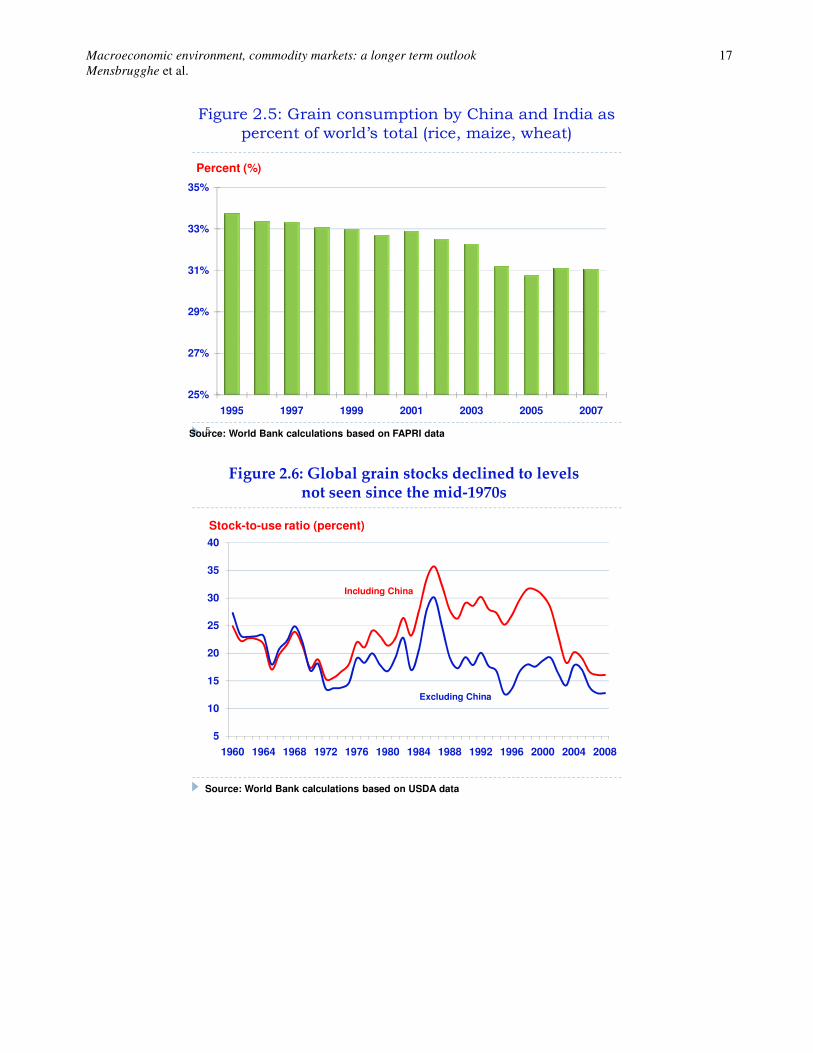
The diversion of considerable quantities of some food commodities for the production of biofuels was a key factor behind the recent boom. Almost 28 percent of US maize area (corresponding to about 1.33 percent of global grain area) was diverted to ethanol production during 2008-09. While the combined maize and oilseed area corresponding to biofuel production corresponds to about 2 percent of global grain and oilseed area, the sharp increase in diversion during the recent 2-3 years came at a time when global grain stocks were at historical lows thus leaving limited room for adjustment by bringing more land into productive uses (see figure 2.6 for historical stock-to-use ratio).

Macroeconomic environment, commodity markets: a longer term outlook 3

Mensbrugghe et al.

When most prices began rallying during the early 2008, many governments faced increased pressure by consumers of key food commodities (especially rice) to contain domestic food price inflation. In response, they imposed various export controls, including exports bans and prohibitive export taxes. While such measures temporarily contained domestic price increases, they further exacerbated world prices increases, especially in the rice market which is very thin (less than 10 percent of global rice production is internationally traded).

In addition to the above factors, increased grain consumption by low and middle income countries (especially China and India) due to rising incomes and changing diets (from grain to meat consumption) has often been cited as key reason that fueled the boom, including the 2008 rally. Yet, as figures 2.4 and 2.5 indicate the combined grain consumption (both for human and animal use) by China and India increased only slightly after 1995, a period during which both countries enjoyed strong economic growth. More importantly, grain consumption in these two countries declined during 1995-2007 if expressed as a share of global consumption. This should not be surprising in view of the low income elasticity of grains even at low per capita incomes (see table 2.1).

III. THE ENERGY/NON-ENERGY PRICE LINK

It has become increasingly clear that the energy price increases of the last few years will reshape not only energy markets but most other markets, including agriculture. For almost 20 years, the price of crude oil averaged about $20 per barrel (real 2000 terms). Most analysts and researchers now believe that the “new” equilibrium price of oil will be at three times as much, with proportional changes expected to take place in all other types of energy. High energy prices along with the high energy intensity of most commodities imply that developments in non-energy (especially food) markets will depend on the nature and degree of the energy/non-energy price link. The remaining of this section elaborates on this issue.

The channels through which energy prices affect other commodities are numerous. On the supply side, energy enters the aggregate production function of most primary commodities through the use of various energy-intensive inputs and, often, transportation over long distances, an equally energy demanding process. Some commodities have to go through an energy-intensive primary processing stage. Other commodities can be used to produce substitutes to crude oil (e.g. maize and sugar for ethanol production or edible oils for biodiesel production). In other cases, the main input may be a close substitute to crude oil, such as nitrogen fertilizer which is made directly from natural gas. (The various transmission channels from energy to non-energy prices have been discussed in Baffes (2007, 2009), FAO (2002), and World Bank (2009), among others.)

This section examines the energy/non-energy price link by estimating the following relationship:

log(NON_ENERGYt) = μ + β1log(ENERGYt) + β2log(MUVt) + β3TIME + εt. (see Table 3.1)

NON_ENERGYt denotes the various non-energy US dollar-based price indices at time t, ENERGYt denotes the energy price index, MUVt denotes the deflator, TIME is time trend, and εt denotes the error term; �, β1, β2, and β3 denote parameters to be estimated. Annual data for a number of commodity indices and prices covering the period from 1960 to 2008 are used in the analysis. Although the signs and magnitudes of the coefficients are not dictated by economic theory, β1 and β2 are expected to be positive because energy as well as other goods and services (as reflected by the measure of inflation) constitute key inputs to the production process of all commodities. On the other hand, β3 is expected to be negative, at least for agricultural commodities—consistent with the long-term impact of technological progress on production costs as well as the low income elasticity of most food commodities, especially cereals.

The estimates, presented in table 3.1, indicate that energy prices and to a lesser extent inflation and technological change explain a considerable part of commodity price variability (the adjusted R2 of all regressions averaged 0.85). Specifically, the parameter estimate of the non-energy index (top row of table 3.1) is 0.28, implying that a 10 percent increase in energy prices is associated with a 2.8 percent increase in non-energy commodity prices, in the long run. Three earlier studies—Gilbert (1989), Borensztein and Reinhart (1994), and Baffes (2007)—reported elasticities of 0.12, 0.11, and 0.16, respectively (table 3.2). When the sample of the current analysis is


24-26 June 2009

adjusted to match the samples of these studies, the pass-through coefficient becomes remarkably similar (0.13 and 0.12, and 0.18, respectively).

The transmission elasticity of the non-energy index, however, masks some variations. The highest pass-through elasticity among the sub-indices was in fertilizer, estimated at 0.55, not surprisingly since nitrogen-based fertilizers are made directly from natural gas. Note that the fertilizer and energy price increases during the recent boom were in line with the increases experienced during the first oil shock: from 1973 to 1974 phosphate rock and urea prices increased four-fold and three-fold, very similar to the crude oil price increase during that period, from $2.81 per barrel to $10.97 per barrel.

The agriculture pass-through, estimated at 0.27, reflects a wide-ranging average: beverages (0.38), food (0.27) and raw materials (0.11). Yet, the elasticity estimates of the food price index components fall within a very narrow range: cereals (0.28), edible oils (0.29), and other food (0.22). Similarly, the estimates for the key food commodities fall within a relatively narrow range, from a low of 0.25 in rice to a high of 0.36 in soybeans (Table 3.3).

Three key conclusions emerge from these results. First, most commodities respond strongly to energy prices, a response that appears to strengthen in periods of high prices as confirmed by the fact that the values of the estimated elasticities increase considerably when the recent boom is included in the analysis. The implication is that, for as long as energy prices remain elevated, not only non-energy commodity prices are expected to be high, but analyzing the respective markets requires understanding of the energy markets as well.

Second, while the transmission elasticities were broadly similar, this was not the case with the inflation coefficient the estimates of which varied considerably in terms of sign, magnitude, and level of significance. It was positive and significantly different from zero only for agriculture (and some of its sub-indices) while it was effectively zero for metals and fertilizers. All this implies that the relationship between inflation and nominal commodity prices is much more complex and, perhaps, changing over time. This may not be surprising if one considers that during 1972-80 (a period which includes both oil shocks) the MUV increased by 45 percent while during 2000-08, it increased by half as much. The nominal non-energy price index increase during these two 8-year periods was identical at 170 percent.

Third, the trend parameter estimates are spread over an even wider range compared to energy pass-through and inflation. The non-energy price index, for example, shows no trend at all. Yet, the metal price index exhibited an almost two percent positive annual trend while the agriculture index showed a one percent negative annual trend. Furthermore, the trend parameter estimates of the agriculture sub-indices vary considerably, from 0.08 for raw materials to -3.12 for beverages, a result which confirms Deaton’s (1999, p. 27) observation that what commodity prices lack in trend, they make up in variability. On the other hand, the trend estimate of the food index, -0.71, significant at the 10 percent level, may add another dimension to the debate on the long-term decline of primary commodity prices, often discussed in the context of the Prebisch-Singer hypothesis (see Spraos 1980, among others).

IV. THE MACROECONOMIC ENVIRONMENT

A number of factors will shape the macroeconomic environment and agricultural supply and demand balances over the medium term (through 2030) and the longer term (through 2050). The starting point of any such analysis is demographics. Between 1950 and 2000 the world saw a huge expansion in global population, an increase of some 3.6 billion persons, or a 250 percent rise compared with 1950 (Figure 4.1). Over the next 50 years, the expansion will slow down considerably, with, according to the UN’s medium variant, an increase of 50 percent over 2000, but coming off a much higher base, this still represents a rise of 3 billion persons. The distributional implications of the population rise are also important. There will be nearly no increase in the high-income countries, but yet a 150 percent increase in the least developed countries.1 Many of the least developed

1 Using today’s definition of least developed.


Mensbrugghe et al.

are countries that have been under significant stress to feed their growing population for both natural and man-made reasons. On the other hand high-income countries have both stagnating populations and food demand and robust agriculture. This combination could lead to increased reliance of the least developed countries on food imports, with other developing regions lying somewhere in between—some with surpluses, such as many Latin American countries and others with potentially growing deficits as some in Asia. The bottom line is that agricultural production has to increase at an average rate of 0.8 percent per annum simply to accommodate population growth and in the least developed countries it would have to grow at an average rate of 1.8 percent over the 50-year period.

The economic factors that will determine food supply and balances can be divided into two categories - demand and supply factors, and these of course will be regionally differentiated. Historically, demand has been conditioned by two factors - income growth and shifts in tastes (often derived from income growth), for example a switch from a diet largely based on grains to more reliance on meat- and dairy-based proteins. In most high-income countries, and some developing countries, the income elasticity for food is nearly 0 for many food commodities as saturation points have been reached.2 There is nonetheless a substantial portion of the global population that would potentially demand relatively more food as incomes rise. The World Bank’s most recent estimate of the incidence of poverty in developing countries was around 47 percent (at the $2/day level) in 2005, declining to around 35 percent by 2015. And the intensification of meat and dairy consumption would raise the demand for grain-based feed, in larger proportion than any relative drop in household based grain demand.

Though we regularly project income growth over the medium- and long-term horizons, one should keep in mind that these are strictly scenario-based (or what-if?) projections and not statistically-based projections as are the more standard short-term forecasts of economic growth. Our projections use a hybrid system where in the short- and medium-term we rely more on estimates of potential growth using statistical techniques, but over the longer-term we switch to a more judgmental forecast that relies on two assumptions: 1) long-term per capita growth in high-income countries will slow to 1.0-1.5 percent per annum; and 2) developing countries will converge towards the per capita incomes of the high-income countries, but at different rates.

Our baseline projection has the global economy increasing at an average rate of around 2.9 percent between 2005 and 2050 (Figure 4.2). This breaks out into 1.6 percent for high-income countries and a brisk 5.2 percent for the developing countries. One of the key consequences of this differential in growth rates is that we witness a very large shift in share of global output. In 2005, developing countries had roughly a 20 percent share in global output (at market exchange rates). By 2050, this jumps to about 55 percent. On a per capita basis the growth differential narrows as population growth is near zero in the high-income countries. At market exchange rates, there is a narrowing of the income gap, but it remains substantial. In 2005, per capita incomes were some 20 times higher in high-income countries relative to developing. This ratio drops to 6 by 2050 though varies highly across regions—with a low of 3.5 in East Asia and Pacific and a high of 20 for sub-Saharan Africa.

With average per capita incomes rising by 2.2 percent between 2005 and 2050, an income elasticity of 0.5 would yield an increase in food demand of 1.1 percent to be added to the 0.8 percent increase in population for a total increase of 1.9 percent. This simple estimate may be an overstatement as one would expect income elasticity for food to decline as incomes rise and is already near zero in most high-income countries. On the other hand, counter-balancing factors that would lead to a rise could be increasing demand for meat and dairy and new competition emerging from biofuels.

The factors behind demand growth are likely to be relatively stable compared with supply side variables. Ultimately, supply growth will be driven by the different degrees of intensification (getting more with the same amount of land) and extensification (expanding land under cultivation). The cost and availability of other inputs—notably water—are also important factors, but are more difficult to integrate into the current analysis.

2 One might even argue that demand could even decline as health and environmental concerns lead to changing dietary habits and lower overall food consumption.


24-26 June 2009

Using the latest available FAO data there is significant scope for extensification in many regions of the world (figure 4.3). Whether this potential supply is exploited or not will depend, among other factors, on the affordability of expansion in terms of infra-structure development and the potential negative externalities of expansion (e.g. environmental degradation). Which regions expand land use will also influence changes in the patterns of food trade. For example, Latin America, which has relatively large tracts of productive non-forest land available, could see a fairly rapid expansion of its production and exportable surplus.

The last few decades that has seen a huge increase in world population and yet stagnant or even falling agricultural prices, has been supported by sizeable improvement in agricultural productivity growth (Coelli and Rao 2005 and World Bank 2009), particularly in Asia, but in North America as well. This rapid growth has tapered somewhat more recently. For example yield growth in wheat and rice has declined from around 2 percent between 1965-1999 to less than 1 percent between 2000 and 2008. This is a cause for concern about the future, particularly as this decline has trended well with the decline in expenditures on research and development. There are available opportunities—in part because many regions are well behind the frontier, for example Europe and Central Asia and sub-Saharan Africa and also because the frontier can still be pushed out, notably with state-of-the-art gene-based research and development.

Part of our analysis of long-term trends relies on an analytical framework that allows us to integrate the various components of the description above—demographics, income growth, structural and taste changes, productivity and evolving factor supplies—into a consistent model of the global economy. The World Bank’s model, known as ENVISAGE (ENVironmental Impact and Sustainability Applied General Equilibrium Model), is a dynamic computable general equilibrium (CGE) model (see Appendix 1 for a longer description of the model). It has several advantages. First, it is global with supply/demand balances guaranteed at the global level. Differences between domestic production and demand are met through exporting surpluses or importing to meet deficits. It also encompasses all economic activity. Hence, if a country becomes a net importer of food, it must export more of other commodities. And third, it is based on a consistent microeconomic underpinning facilitating what-if analysis. For example, what if productivity is higher or lower? What if demand for meat and dairy in developing countries follows a different pattern than for the high-income countries? What if energy prices rise? How does this affect the cost-structure of food supply? Will it induce more demand for biofuels? The remainder of this section explores some of these fundamental questions with the assistance of the model.

The baseline scenario, with productivity growth of 2.1 percent per annum in agriculture, yields a benign price pattern for overall agriculture, i.e. there is a small negative trend over the long-term with global supply/demand balances more or less lined-up (Figure 4.4). This has been the pattern for the last 30-40 years. Supply/demand balances at a regional level may widen as some countries have little room for expansion and also see a shift in comparative advantage in other goods. In the absence of new support policies, East Asia could see a relatively large increase in net agricultural imports with the high-income countries and Latin America and the Caribbean having exportable surpluses (figure 4.5).

Assumptions regarding productivity, as noted earlier, are key to determining potential stress on food markets. To assess the impact of the baseline assumption on agricultural productivity, two additional scenarios are undertaken. In the first scenario, developing countries are assumed to have half the productivity growth in agriculture compared with the baseline assumption. This could be driven by a number of factors including failure to ramp up research and development expenditures, resistance to genetically modified organism (GMO) technology, reduced effectiveness of inputs, lower land productivity (due to increasing salinity for example) or inadequate supply of water. The model suggests that in this case global agricultural prices would rise modestly compared to today’s levels. However, it would also increase developing countries reliance on agricultural imports—with again rising dependence in Asia. Latin America and Caribbean remains as a net agricultural exporter.

If global productivity is halved, then agricultural prices rise by significantly more, nearly 35 percent above the base year in 2030 as compared with about 16 percent when only developing country agriculture is subjected to the lower productivity growth. The impact on trade balances is more mixed—lying in most cases between the


Mensbrugghe et al.

baseline levels and the scenario where only developing country agriculture is impacted. Note that the net trade numbers are in value terms so that part of the change in the net trade will be induced by the change in the higher agricultural prices and is not simply a volume phenomenon.

V. CLIMATE CHANGE

One issue that might be looming large in the next few decades is the impact of climate change on global

agriculture. Some estimates suggest that a rise of 2.5 ⁰C could lower agricultural productivity by up to 40

percent, including in some very large countries such as India (Cline 2007). The net impact of climate change on agriculture is still being debated—at least at the global level. Some regions, notably the higher latitudes could benefit from longer growing periods, largely offsetting the damage in regions in the lower latitudes. There is also uncertainty regarding the impact of carbon fertilization. There is some evidence that higher concentrations of carbon may induce growth, at least to a certain point, and this could also potentially offset higher temperatures. Finally, though the general circulation models (GCMs) have a relatively high degree of consistency regarding temperature increases, there is much less consensus on rain patterns and the overall supply of water for agricultural purposes.

One of the features of the ENVISAGE model is that it incorporates the full cycle of greenhouse gas emissions from human activities, atmospheric concentrations and radiative forcing and changes in temperature. This class of models is also known as an Integrated Assessment Model (IAM). The model also couples changes in global temperature to economic damages. Currently, damages are only incurred in agriculture through impacts on agricultural productivity.

Figure 4.6 depicts how climate-induced agricultural damages are allocated across the globe based on the estimates produced by Cline. The figure clearly shows the concentration of damages in the lower latitudes and largely for developing countries. It represents in some sense a ‘worse’ case scenario in that it represents the damage estimates in the absence of the carbon fertilization effect. For the purposes of the baseline scenario, the damages have been assumed to be the average of the with- and without carbon fertilization effect. Cline’s

estimates are based on the assumption that the increase in temperature of 2.5 ⁰C will occur around 2080. This is

based on scenarios developed at the end of the 1990s that have assumed a lower profile of emissions than that have been observed over the last decade, the current crisis notwithstanding. The damage functions in

ENVISAGE are calibrated to Cline’s estimated impacts for a temperature change of 2.5 ⁰C. For technical

reasons we have specified and calibrated linear damage functions. This may overstate damages in the short-term, particularly in certain regions where warming could be beneficial, for example the higher latitudes, and understate damages in the long-run as many damage functions in the literature are assumed to be non-linear (see Nordhaus 2008 for example).

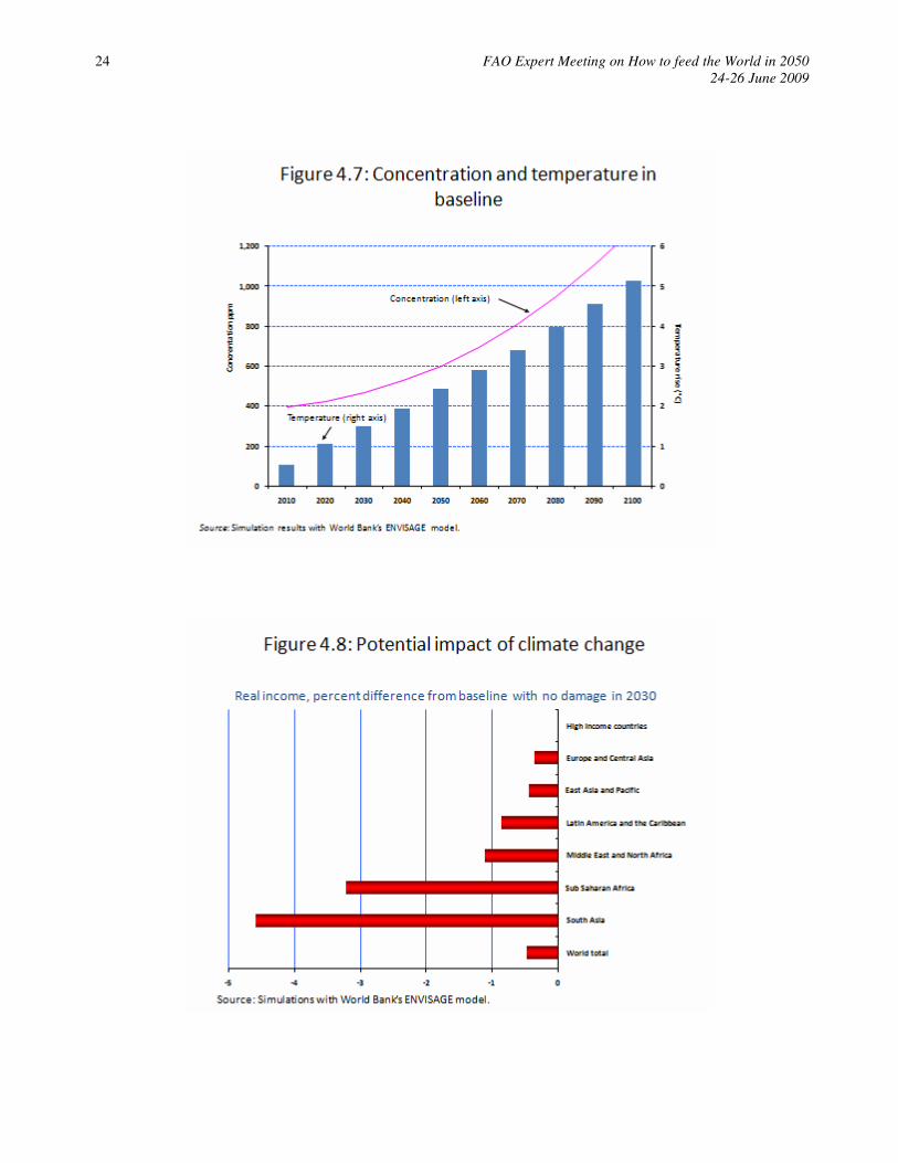
For the purposes of climate analysis the model runs through 2100, however for the purposes of this paper the focus will continues to be on the period that ends in 2030. In terms of atmospheric emissions, our projected emissions profile is significantly higher than most of those that form the basis of the climate change analysis as recently presented in the Fourth Assessment Report (AR4) of the Intergovernmental Panel on Climate Change (IPCC 2007). The scenarios in AR4 were generated around 2000 and largely underestimated both output and emission growth over the last decade. As a result, our baseline scenario shows much greater emission growth, and, if this pattern continues, puts the world on a trajectory with much higher temperature changes than the AR4 median of around 3 °C by the end of the century (Figure 4.7). With a higher temperature profile than the AR4 median, our estimates of the impacts from climate change on agriculture occur much earlier than assumed in the

Cline study as the 2.5 ⁰C level is reached in 2050 and not in 2080.

The climate damages are built into the standard baseline. To isolate the impact of climate change an alternative scenario is simulated where the climate change damages are assumed away. All other exogenous assumptions are the same between the two scenarios. In this alternative scenario, agricultural productivity matches the exogenous assumption of 2.1 percent uniform growth with no deviation. The impacts on real income from


24-26 June 2009

climate damages even in 2030 could be substantial. South Asia would take the most significant hit—a loss in real income in 2030 of over 2 percent, more than double the loss of the next region, sub-Saharan Africa (Figure 4.8). The relatively large losses in these two regions reflect two factors. First, agriculture remains important despite relatively rapid economic growth. Second, the fact that existing studies suggest that the largest damages are occurring in these two regions – as summarized in Cline’s (2007) estimates.

Finally, in this alternative scenario, the impact on high-income countries is negligible in the short-term. Partly, this arises from gains in the terms of trade as world prices rise in the with-damage scenario. The net trade position of all developing regions deteriorates in the with-damage scenario, albeit somewhat modestly in 2030, and improves (modestly) for high-income countries. In the long-run climate damages are bound to increase both because the climate will deteriorate and also due to non-linear effects (not currently captured in our model).

Biofuels

The expansion of ethanol based on grain feedstock is quite different from that of sugar cane-based ethanol, especially in Latin America. In the later the tradeoff between food and fuel is quite limited. Moreover, sugarcane expansion would occur primarily in Latin America and then in other countries with low-cost sugar production. Most of this expansion will occur on land for which competition among crops is limited. By contrast, ethanol based on grains has a direct effect on several important competing crops, including oilseeds. The expansion of biodiesel as a strong and direct implication for vegetable oil prices and the feedstock and food demand are in direct competition. A large biodiesel expansion will push vegetable prices higher. Hence, the expansion of biofuel based on grains and oilseed products is a potential exacerbating factor for higher food prices and could compromise the access to food for the poorest on the planet. The most affected food prices would be grains, vegetable oils, meat, and dairy products which are intensive in feedstocks.

If cellulosic/biomass ethanol can become profitable, the tradeoff between food and fuel may be less important and confined to oilseed based biofuels. The development of biofuels is also determined by their return. The latter is largely determined by fossil energy prices and feedstock prices. Low fossil energy prices will undermine the development of large biofuel sectors and would reduce the tradeoff between food and fuel. Of course large and forced biofuel mandates could change this result. It is difficult to know what policies will prevail in 2050. Biofuels, both first and second generation, are currently being implemented in the model and will form the basis of further analysis.

VI. POVERTY IMPLICATIONS

We have used the assumptions in the baseline scenario explained in section V to “roll” the global economy to 2050. In this section we’ll concentrate on the global distributional effects behind the expected changes in per capita incomes and its distribution within countries3. To evaluate these distributional effects we rely on the World Bank’s Global Income Distribution Dynamics (GIDD) model. The GIDD, a macro-micro simulation framework, is overviewed in Box 3 and explained in full detail in Bussolo, de Hoyos, and Medvedev (2008).

Figure 6.1 below plots Lorenz curves for the observed global income distribution in 2005 and the projected distribution in 2050. It appears that the largest changes in income distribution between 2005 and 2050 are expected to be found around the middle of the income distribution rather than towards the upper or lower tails. In fact, because the two Lorenz curves intersect in these tails, it is not possible to say that the 2050 distribution Lorenz-dominates that of 2005. In other words, we cannot claim that inequality in 2050 is lower as compared with 2005 regardless of the inequality measured being used. However, using standard inequality statistics such

3 This section has been prepared relying on the methodology used in Bussolo et. al (2007) where the global economy was projected to 2030. Nevertheless, it has some minor variations: we are using the latest version of the GIDD (June, 2009) that has 2005 as a base year – instead of year 2000, and uses the latest Purchasing Power Parity conversion factors. As a result, slightly differences may emerge between the two documents, but these differences will not compromise the messages and authors’ conclusions in any of them.


Mensbrugghe et al.

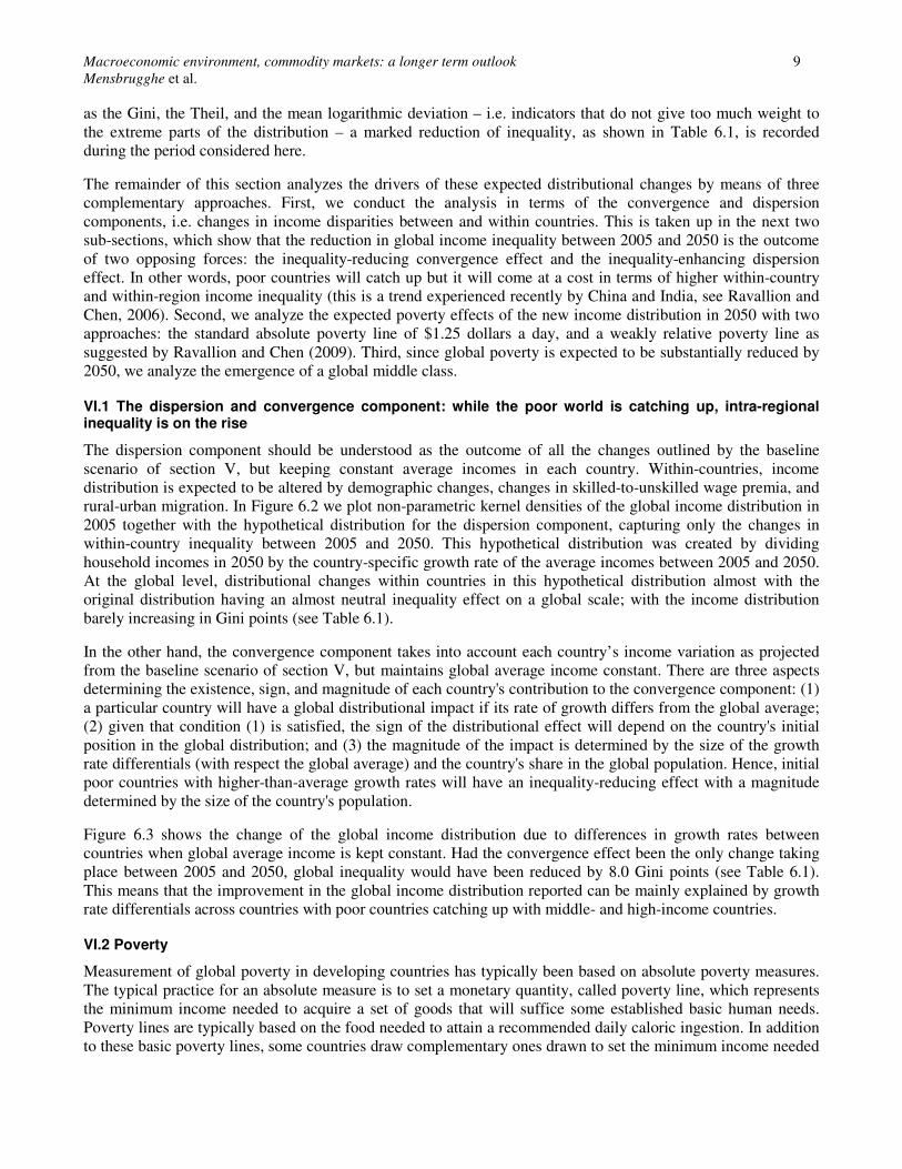
as the Gini, the Theil, and the mean logarithmic deviation – i.e. indicators that do not give too much weight to the extreme parts of the distribution – a marked reduction of inequality, as shown in Table 6.1, is recorded during the period considered here.

The remainder of this section analyzes the drivers of these expected distributional changes by means of three complementary approaches. First, we conduct the analysis in terms of the convergence and dispersion components, i.e. changes in income disparities between and within countries. This is taken up in the next two sub-sections, which show that the reduction in global income inequality between 2005 and 2050 is the outcome of two opposing forces: the inequality-reducing convergence effect and the inequality-enhancing dispersion effect. In other words, poor countries will catch up but it will come at a cost in terms of higher within-country and within-region income inequality (this is a trend experienced recently by China and India, see Ravallion and Chen, 2006). Second, we analyze the expected poverty effects of the new income distribution in 2050 with two approaches: the standard absolute poverty line of $1.25 dollars a day, and a weakly relative poverty line as suggested by Ravallion and Chen (2009). Third, since global poverty is expected to be substantially reduced by 2050, we analyze the emergence of a global middle class.

VI.1 The dispersion and convergence component: while the poor world is catching up, intra-regional inequality is on the rise

The dispersion component should be understood as the outcome of all the changes outlined by the baseline scenario of section V, but keeping constant average incomes in each country. Within-countries, income distribution is expected to be altered by demographic changes, changes in skilled-to-unskilled wage premia, and rural-urban migration. In Figure 6.2 we plot non-parametric kernel densities of the global income distribution in 2005 together with the hypothetical distribution for the dispersion component, capturing only the changes in within-country inequality between 2005 and 2050. This hypothetical distribution was created by dividing household incomes in 2050 by the country-specific growth rate of the average incomes between 2005 and 2050. At the global level, distributional changes within countries in this hypothetical distribution almost with the original distribution having an almost neutral inequality effect on a global scale; with the income distribution barely increasing in Gini points (see Table 6.1).

In the other hand, the convergence component takes into account each country’s income variation as projected from the baseline scenario of section V, but maintains global average income constant. There are three aspects determining the existence, sign, and magnitude of each country's contribution to the convergence component: (1) a particular country will have a global distributional impact if its rate of growth differs from the global average; (2) given that condition (1) is satisfied, the sign of the distributional effect will depend on the country's initial position in the global distribution; and (3) the magnitude of the impact is determined by the size of the growth rate differentials (with respect the global average) and the country's share in the global population. Hence, initial poor countries with higher-than-average growth rates will have an inequality-reducing effect with a magnitude determined by the size of the country's population.

Figure 6.3 shows the change of the global income distribution due to differences in growth rates between countries when global average income is kept constant. Had the convergence effect been the only change taking place between 2005 and 2050, global inequality would have been reduced by 8.0 Gini points (see Table 6.1). This means that the improvement in the global income distribution reported can be mainly explained by growth rate differentials across countries with poor countries catching up with middle- and high-income countries.

VI.2 Poverty

Measurement of global poverty in developing countries has typically been based on absolute poverty measures. The typical practice for an absolute measure is to set a monetary quantity, called poverty line, which represents the minimum income needed to acquire a set of goods that will suffice some established basic human needs. Poverty lines are typically based on the food needed to attain a recommended daily caloric ingestion. In addition to these basic poverty lines, some countries draw complementary ones drawn to set the minimum income needed


24-26 June 2009

to suffice more complex human needs i.e. health and education. At the global level, the World Bank’s “$1 and $2-a-day” are the best known example of absolute poverty lines.

Alternatively, the common practice in OECD countries is to use relative poverty lines. These monetary quantities are periodically adjusted, not as the minimum income needed to acquire a given basket of goods, but as a constant proportion of the countries’ mean or median incomes. The first argument to use relative poverty measures over absolute ones relies on the “welfarist” assumption that people attach value to their own income relative to the average in its own society – often cited as the “theory of relative deprivation” or the “relative income hypothesis”. The second argument in favor of relative poverty lines is that they allow for differences in the cost of social inclusion. Following Ravallion and Chen (2009) these are defined as the expenditure needed to cover certain commodities that are deemed to have a social role in assuring that a person can participate with dignity in customary social and economic activities.

Despite the two cited arguments in favor of relative rules to measure poverty trends, they have not been used for the study of poverty in very low income countries because they possess the property of scale independency, in other words, if all incomes in a society grow at the same rate, no change in poverty will occur.

Ravallion and Chen (2009) discuss all these aspects rigorously and outlined an alternative measure. With the use of a large sample of poverty lines collected by the World Bank, they calibrate a new measure for the study of global poverty called weakly poverty line. The proposed weakly relative poverty line is, in general terms, a combination of the two previous approaches: (1) For very low levels of income, it functions as an absolute poverty line set to the World Bank’s $1.25 a day (in purchasing power parities of 2005). (2) For medium and higher incomes, it functions as a relative poverty line. The empirical implementation followed the formula:

(5.1)

where Zi is the value of the poverty line, Mi is the mean daily income in country i, and α was estimated by Ravallion and Chen (2009) to be PPP $0.60. The advantage of using the weakly relative poverty line is that it will provide a better understanding about poverty and exclusion in the projected income distribution in 2050 than the absolute poverty measure. Table 6.2 summarizes the regional headcount ratio of absolute and weakly relative poverty in 2005 and 2050. While absolute poverty vanishes in the planet, weakly relative poverty still accounts for a large share of the population, especially in underperforming Latin America. According to our baseline scenario, the increase in weakly relative poverty reported by Ravallion and Chen (2009) experienced during the late 1980s and until the year 2000 is reversed by year 2050 in almost all regions. Table 6.2 shows the headcount index for absolute and weakly relative poverty in 2005 and 2050 as well as the change in the number of poor in both periods.

The most interesting result is that while other nations are performing relatively well, Latin America is the only region where the number of weakly relative poor actually increases (67 million), partly reflecting that it is the most unequal region in the planet. Within Latin America and the Caribbean, the only countries that have a net reduction in the number of relative poor are Guyana, Peru, and Haiti with a joint reduction of 4.5 million. All other countries will see the number of relative poor increasing, Mexico being the most affected. Mexico alone accounts for half of the increase in the number of relative poor in Latin America, followed by Brazil (11 million), Ecuador (4.8 million), and Colombia (4 million).

In sub-Saharan Africa, absolute poverty is expected to be reduced from 51.2 to 2.8 percent of the population; and remarkably, weakly poverty from 55.5 to 20.3 percent of the population. The country that will perform the better is United Republic of Tanzania that will reduce in almost 70 percent its relative poverty rate with an absolute negative change of 20 million living in relative poverty. In addition, Nigeria and Ethiopia will reduce drastically the net number of poor in 34 and 20 million respectively; but in relative terms, the best performers are Malawi, Burundi, Guinea, and Rwanda; all of them with relative poverty reduction rates above the 50 percent points.


Mensbrugghe et al.

VI.3 The new middle class and beyond

Alternatively to the study of global poverty, the emergence of countries in the new middle class is of high importance because the expected changes in global consumption patterns accompanied by economic growth. Certainly, individuals in 2050 will be healthier and more educated, with higher expectations about their role in life, greater political participations, and increasingly more complex needs. As a result, the demand for more and better goods and services will rise as vast number of families emerges from poverty in developing countries. Bussolo et al., (2007) uses a definition of absolute global middle class (GMC) that we will use in order to quantify the number of people that will be part of this group in the hypothetical income distribution in 2050. The GMC will be defined as the world citizens living with incomes between the current Brazilian and Italian averages.

The GMC will grow from around 450 million in 2005 to 2.1 billion in 2050, and from 8.2 to 28.4 percent of the global population (Table 6.3). Furthermore, the composition of this group of consumers is likely to change radically: while in 2005, developing country nationals accounted for 56 percent of the GMC, by 2050 they are likely to represent nearly the totality of this group. The biggest contributors to the increase in the number of the GMC members are the most populous Asian countries led by China and India. These two countries alone are responsible for nearly two-thirds of the entire increase in the GMC, with China accounting for 30 percent of the rise in the GMC population and India adding another 35 percent. More surprisingly is that as a result of the sustained economic growth in China and according to the scenario depicted in section V, by 2050, 40 percent of the Chinese population will surpass the global middle class status.

There are several reasons behind the dramatic increase projected in the size of the GMC and the major shift in composition in favor of the low- and middle-income countries. Faster population growth in the developing world is responsible for some of the change in the composition. Thus regions with population growth above the world average (for example, South Asia and sub-Saharan Africa) will increase their share in the global middle class. The main determinant of joining the middle class ranks, however, is not population growth but income growth. Although East Asia’s population grows more slowly than the world average, this region is projected to increase its share of residents in the global middle class by more than 30 percent points, compared with 15 percent points in sub Saharan Africa. The difference is due to the fact that annual per capita income growth in Asia is forecasted to be more than twice the growth in sub-Saharan Africa, easily offsetting the decline in the former’s population share.

Most developing-country members of today’s (as of 2005) global middle class earn incomes far above the averages of their own countries of residence. In other words, being classified as middle class at the global level is equivalent to being at the top of the distribution in many low-income countries. For example, in our sample, as of 2005, 180 million (out of the total 260 million) developing country citizens in the global middle class are in the top 20 percent of earners within their own countries. Thus, for many nations, the correspondence between the global middle class and the within-country middle class is quite low. The situation will change quite dramatically by 2050. A full 60 percent of developing country members of the global middle class will be earning incomes in the seventh decile or lower at the national level. Consider the example of China, where 27 million people belonged to the global middle class in 2005—each of them earning more than 90 percent of all Chinese citizens. By 2050, there will be 517 million Chinese in the global middle class, and their earnings will range from the fifth to the ninth decile of the Chinese national income distribution.

Consistent with these data, by 2050 the middle class, together with the rich, will account for a larger share of the population in a greater number of countries. In 2005, the members of middle class and the rich group exceeded 40 percent of the population in only six developing countries (Azerbaijan, Chile, Costa Rica, Hungary, Mexico, and Uruguay) these countries were home to 3.0 percent of the population of the developing world. By 2050, the middle class and the rich will exceed 40 percent of the population in 58 developing countries (as they are classified today), and these countries will account for 72 percent of the world’s developing country population.


24-26 June 2009

VII. CONCLUSIONS

At a minimum, the price spikes of 2007-2008 shook global complacency as regards agriculture after a period of neglect driven in part by globally benign price changes and no major supply disruptions. Experts were aware about the fall in agricultural productivity growth and expenditures on research and development, but in a crowded field of international economic policy issues, the warning signs were largely ignored. As regards agriculture, the focus has been much more on farm support policies and trade barriers than on fundamental supply issues. Are we now witnessing a structural shift, with higher and growing agricultural prices, or was 2007-2008 just a bump in the road. This paper suggests that the answer lies somewhere in between. There is a structural shift with a greater linkage to energy markets than in the past. Higher energy prices could induce a stronger shift to biofuels with competing pressures on resources and higher food prices. Potentially this linkage could be strengthened if climate mitigation policies raise the end-use price of conventional fossil fuels and induce a further substitution into biofuels. At the same time, there are reasons to believe that the world can adjust to these imminent changes. Declining population growth and food saturation will temper food demand growth in the future and health and environmental concerns could even induce a shift in tastes that would temper demand even further. There is also sufficient land that would allow for some expansion, if managed appropriately and sustainably. It will require investment in infrastructure, which could be onerous, particularly in the poorer parts of the world. The ability to raise productivity is also a concern, particularly in an environment with growing climate stress. Again, it will require resources to enhance research and development, with perhaps an emphasis on regions where productivity lags far behind best practices.

However, even if there is manageable stress at the global level, the changing environment at a regional level is likely to have distributional repercussions both across and within countries. Managing these stresses may be more difficult as food security at both the household and national level are often priorities for policy makers. And as we witnessed in the most recent crisis, policy makers, naturally, will make the most rational decisions for their stakeholders even if better overall policies could be implemented with the right coordination.


Mensbrugghe et al.

BOX 1: Experience with Managing Commodity Markets The long-term declines along with high variability of commodity prices prompted many governments to take collective measures to either prevent the decline or reduce the variability. Coffee producers, led by Brazil, organized the 1962 International Coffee Agreement (and a subsequent series of agreements) to restrict exports and boost coffee prices. Similar efforts were undertaken by cocoa producers while attempts were also made in other markets (e.g. cotton, grains). The oil producers formed the Organization of Petroleum Exporting Countries (OPEC) in 1960 in order to raise prices through supply controls. Similarly, buffer stocks were used by organizations of commodity producing countries in order to stabilize prices. Tin producers, through the International Tin Agreement managed buffer stocks to maintain prices within a range. The International Cocoa Agreement, form in 1972, also attempted to stabilize prices through buffer stocks but was suspended in 1988. The International Natural Rubber Organization was formed to stabilize rubber prices but major producers withdrew from the Organization following the East Asia financial crisis of 1997. With the exception to OPEC, all these agreements failed to achieve their stated objectives as coordination and monitoring among many sovereign nations turned out to be a difficult task. In addition to the post-WWII commodity agreements, there was another wave of agreements that were formed in response to the low prices following the Great Depression.

BOX 2: The Role of Speculation during the Recent Commodity Boom Since 2003 index fund investors, who allocate funds across a basket of commodities by taking long positions various commodities traded in organized futures exchanges, have invested almost $250 billion in U.S. commodity markets, about half of it in energy commodities (Masters 2008). While such transactions are not associated with real demand for commodities, they may have influenced prices for a number of reasons. First, because investment in commodities is a relatively new phenomenon, there have been mostly inflows (not outflows) of funds implying that some markets may have been subjected to extrapolative price behavior (i.e., high prices leading to more buying by investment funds consequently leading to even higher prices, and so on). Second, these funds invest on the basis of fixed weights or past performance criteria and hence investment often takes places in contrast to what market fundamentals would dictate. Third, the large size of these funds compared to commodity markets may exacerbate price movements. Their influence on prices is especially likely, if the rapid expansion of these markets contributed to expectations of rising prices, thereby exacerbating swings, as argued by Soros (2008, p. 4) who called commodity index buying “... intellectually unsound, potentially destabilizing and distinctly harmful in its economic consequences.” Similar views are shared by numerous authors (see for example, Eckaus (2008) and Wray (2008)).

Yet, the empirical evidence on whether such funds contributed to the price boom has been, at best, mixed. In the non-ferrous metal market, Gilbert (2008) found no direct evidence of the impact of investor activity on the prices of metals but some evidence of extrapolative price behavior that resulted in price movements not fully justified by market fundamentals. He also found strong evidence that futures positions of index providers over the past two years have affected the soybean (but not the maize) prices in the US futures exchanges. Plastina (2008) concluded that between January 2006 and February 2008, investment fund activity might have pushed cotton prices 14 percent higher than what would have been otherwise. On the other hand, two IMF (2006, 2008) studies failed to find evidence that speculation has had a systematic influence on commodity prices. A similar conclusion was reached by a series of studies undertaken by the Commodities Futures Trading Commission, the agency that regulates U.S. futures exchanges (Büyük�ahin, Haigh, and Robe 2008; CFTC 2008).

Although the empirical evidence regarding the effect of investment fund activity is mixed and inconclusive, the large amount of money that does into commodities certainly has an effect on prices, which is the consensus among experts. On the other hand, market fundamentals will determine the long-term trends of commodity prices, which implies that investment fund activity has induced higher price variability.


24-26 June 2009

BOX 3: The Global Income Distribution Dynamics model

The World Bank Development Economics Prospects Group (DECPG) has developed the Global Income

Distribution Dynamics (GIDD), the first global CGE-microsimulation model. The GIDD takes into account the

macro nature of growth and of economic policies and adds a microeconomic—that is, household and

individual—dimension to it.

The GIDD includes distributional data for 121 countries and covers 90 percent of the world population. Academics and development practitioners can use the GIDD to assess growth and distribution effects of global policies such as multilateral trade liberalization, policies dealing with international migration and climate change, among others. The GIDD also allows analyzing the impacts on global income distribution from different global growth scenarios and to distinguish changes due to shifts in average income between countries from changes attributable to widening disparities within countries.

The macro-micro modeling framework described here explicitly considers long-term time horizons during which changes in the demographic structure may become a crucial component of both growth and distribution dynamics. The GIDD’s empirical framework is schematically represented in the figure to the left. The expected changes in population structure by age (upper left part of the figure) are exogenous, meaning that fertility decisions and mortality rates are determined outside the model. The change in shares of the population by education groups incorporates the expected demographic changes (linking arrow from top left box to top right box in the figure). Next, new sets of population shares by age and education subgroups are computed and household sampling weights are re-scaled according to the demographic and educational changes above (larger box in the middle of the figure). The impact of changes in the demographic structure on labor supply (by skill level) is incorporated into the CGE model, which then provides a set of link variables for the micro-simulation:

(a) change in the allocation of workers across sectors in the economy, (b) change in returns to labor by skill and occupation, (c) change in the relative price of food and non-food consumption baskets, and (d) differentiation in per capita income/consumption growth rates across countries.

The final distribution is obtained by applying the changes in these link variables to the re-weighted household survey (bottom link in the figure).


Mensbrugghe et al.

Figure 2.1: Unlike earlier booms, the currentboom involved all commodity groups

0

50

100

150

200

250

300

350

1948 1953 1958 1963 1968 1973 1978 1983 1988 1993 1998 2003 2008

Real MUV-deflated, 2000=100

Agriculture

Energy

Source: World Bank

Metals

Korean

war

Oil

shocks

Recent

boom

Figure 2.2: All commodity prices have declinedsharply since the mid-2008

0

100

200

300

400

500

Jan-00 Jan-02 Jan-04 Jan-06 Jan-08

Energy Agriculture Metals

Nominal price indices (2000=100)

Source: World Bank


24-26 June 2009

Figure 2.3: Investment by major multinational oilcompanies follows energy prices

Source: International Energy Agency and World Bank

0

50

100

150

200

250

30

60

90

120

150

180

1981 1984 1987 1990 1993 1996 1999 2002 2005

US investment in Oil & Gas (Real 2006, US$ billion) [left]

Energy Price Index (Real 2000=100) [right]

Figure 2.4: Total grain consumption by China and India(rice, maize, wheat)

Source: World Bank calculations based on FAPRI data

300

350

400

450

500

550

600

1995 1996 1997 1998 1999 2000 2001 2002 2003 2004 2005 2006 2007

Million tons


Mensbrugghe et al.

��

�� !� �� "

Source: World Bank calculations based on FAPRI data

25%

27%

29%

31%

33%

35%

1995 1997 1999 2001 2003 2005 2007

Percent (%)

5

5

10

15

20

25

30

35

40

1960 1964 1968 1972 1976 1980 1984 1988 1992 1996 2000 2004 2008

Stock-to-use ratio (percent)

Including China

Excluding China

Figure 2.6: Global grain stocks declined to levels not seen since the mid-1970s

Source: World Bank calculations based on USDA data


24-26 June 2009

��#��$%�� &� ��

� �'��

7

“Speculators”

Speculators in futures

exchanges

Important entities for the functioning

of the futures market as they undertake risk

Speculators who “corner”

markets

Isolated cases such as the cornering of

the copper and silver markets

Hedge funds and short

term trading

Short term profit seeking, often

associated with short term price

volatility

Stockholding activity by

speculators

Hoarding of commodities

expecting that price increases will

generate profits

Investment, pension, and wealth funds

Fund managers invest in long term futures contracts to diversify their

portfolio

Source: World Bank

TABLE 2.1: INCOME ELASTICITIES

Low Income Lower Middle Income Upper Middle Income High Income

Grains 0.15 0.10 0.05 -0.01

Vegetable Oils 0.50 0.65 0.78 0.41

Meats 0.31 0.51 0.68 0.38

Notes: The estimates are based on panel estimation.

Source: Authors’ estimates.


Mensbrugghe et al.

TABLE 3.1: PARAMETER ESTIMATES, PRICE INDICES

INDEX μ ββββ1 ββββ2 100*ββββ3 Adj-R2 ADF

Non-Energy 3.03@ (6.54)

0.28@ (5.24)

0.12 (0.68)

-0.01 (0.02)

0.90 -3.35**

Metals 3.77@ (4.80)

0.25@ (3.14)

-0.17 (0.60)

1.93@ (2.31)

0.82 -3.30**

Fertilizers 3.58@ (4.12)

0.55@ (4.79)

-0.30 (0.95)

0.39 (0.48)

0.81 -3.97***

Agriculture 2.51@ (6.90)

0.26@ (5.54)

0.33@ (2.43)

-0.99@ (2.73)

0.90 -3.81***

Beverages 1.83@ (3.10)

0.38@ (4.87)

0.55@ (2.63)

-3.12@ (5.22)

0.76 -4.95***

Raw materials 1.85@ (4.16)

0.11@ (2.15)

0.51@ (3.15)

0.08 (0.19)

0.91 -3.15**

Food 2.91@ (7.11)

0.27@ (4.93)

0.21 (1.39)

-0.71 (1.80)

0.85 -3.85***

Cereals 3.13@ (5.94)

0.28@ (4.23)

0.17 (0.89)

-0.87 (1.76)

0.78 -3.83***

Edible oils 3.33@ (6.16)

0.29@ (4.51)

0.12 (0.58)

-0.80 (1.50)

0.80 -2.82*

Other food 1.86@ (6.28)

0.22@ (3.81)

0.45@ (4.44)

-0.42 (1.18)

0.89 -3.60***

Precious metals -1.40@ (3.58)

0.46@ (9.40)

1.05 (7.61)

-1.75 (3.68)

0.98 -3.91***

Notes: The @ sign denotes parameter estimate significant at the 5 percent level while the numbers in parentheses are absolute t-values (the corresponding variances have been estimated using White’s method for heteroskedasticity-consistent standard errors.) ADF denote the MacKinnon one-sided p-values based on the Augmented Dickey-Fuller equation (Dickey and Fuller 1979). One (*), two (**), and three (***) asterisks indicate rejection of the existence of one unit root at the 10 percent, 5 percent, and 1 percent levels of significance (the respective t-statistics are -2.60, -2.93, and -3.58). The lag length of the ADF equations was determined by minimizing the Schwarz-loss function.

Source: Author’s estimates.


24-26 June 2009

TABLE 3.2: COMPARING LONG-RUN TRANSMISSION ELASTICITIES

Holtham (1988)

1967:S1-1984:S2

Gilbert (1989)

1965:Q1-1986:Q2

Borensztein &

Reinhart (1994)

1970:Q1-1992:Q3

Baffes (2007)

1960-2005

This Study

1960-2008

Non-energy — 0.12 0.11 0.16 0.28

Food — 0.25 — 0.18 0.27

Raw materials 0.08 — — 0.04 0.11

Metals 0.17 0.11 — 0.11 0.25

Notes: Holtham uses semiannual data, Gilbert and Borensztein & Reinhart quarterly, and Baffes along with the present study annual. Gilbert’s elasticities denote averages based of four specifications. Holtham’s raw materials elasticity is an average of two elasticities based on two sets of weights. ‘—‘ indicates that the estimate is not available.

Source: Holtham (1988), Gilbert (1989), Borensztein and Reinhart (1994), Baffes (2007), and author’s estimates.

TABLE 3.3: PARAMETER ESTIMATES, INDIVIDUAL COMMODITIES

COMMODITY μ ββββ1 ββββ2 100*ββββ3 Adj-R2 ADF

Wheat 3.27@ (6.50)

0.30@ (5.02)

0.12 (1.49)

-0.49 (1.07)

0.84 -4.35**

Maize 3.15@ (6.23)

0.27@ (4.66)

0.13 (0.70)

-0.74 (1.58)

0.80 -3.49**

Soybeans 3.58@ (8.11)

0.26@ (4.92)

0.25 (1.51)

-0.82 (1.83)

0.82 -3.85***

Rice 3.57@ (5.14)

0.25@ (2.67)

0.32 (0.26)

-1.62@ (2.78)

0.58 -4.05***

Palm oil 4.94@ (6.44)

0.35@ (3.72)

-0.01 (0.02)

-0.95 (1.38)

0.63 -3.16**

Soybean oil 5.25@ (7.83)

0.36@ (4.13)

-0.09 (0.39)

-0.42 (0.53)

0.70 -2.56

Notes: See table 3.1


Mensbrugghe et al.


24-26 June 2009


Mensbrugghe et al.


24-26 June 2009


Mensbrugghe et al.

020

40

60

80

100

Cum

ula

tive

Inco

me S

hare

(%

)

0 20 40 60 80 100Cumulative % of Population

Distribution 2005 Distribution 2050

Figure 6.1 Lorenz Dominance: Changes in

the middle of the distribution

Source: Authors’ calculations

Source: Authors’ estimates

Table 6.1 Global Income Inequality

Dispersion Convergence

Index 2005 2050 Only Only

Gini 0.697 0.616 0.701 0.616

Theil 1.046 0.717 1.059 0.719

Mean Log Deviation 0.942 0.723 0.954 0.723

Gini Theil Mean Log Dev

Region 2005 2050 2005 2050 2005 2050

Developed Countries 0.394 0.378 0.270 0.245 0.277 0.257

Developing Countries 0.552 0.588 0.623 0.664 0.529 0.629

East Asia and the Pacific 0.421 0.479 0.311 0.399 0.293 0.411

Eastern Europe and Central Asia 0.394 0.513 0.257 0.441 0.280 0.490

Latin America and the Caribbean 0.599 0.605 0.714 0.707 0.699 0.719

Middle East and North Africa 0.399 0.405 0.284 0.298 0.261 0.271

South Asia 0.297 0.326 0.156 0.183 0.141 0.176

Sub Saharan Africa 0.495 0.488 0.499 0.481 0.425 0.410

Data source: Authors' estimates


24-26 June 2009

0.697

1.046

0.942

0.616

0.717 0.723

0

0.2

0.4

0.6

0.8

1

1.2

Gini Theil Mean Lod Deviation

2005 2050

Figure 6.2 Global Income Inequality reduction, while…


0

0.1

0.2

0.3

0.4

0.5

0.6

0.7

EAP ECA LAC MNA SAS SSA DEV

2005 2050

Figure 6.3 Within-region income inequality on the rise



Mensbrugghe et al.

Figure 6.4 Income distribution in 2005 and 2050:

Reduction of absolute poverty

0

.1

.2

.3

.4

De

nsi

ty

0 2 4 6 8 10Monthly household per capita income (2005 PPP, log)

$1.25 poverty lne


-100

0

100

200

300

400

500

600

700

EAP ECA LAC MNA SAS SSA

Change in Absolute Poor Change in Relative Poor


Figure 6.5 Reduction in absolute vs relative poverty

Relative Poverty Measured as Ravallion and Chen (2009) “Weakly Relative Poverty”


24-26 June 2009

Table 6.2 Poverty Estimates Absolute Poverty ($1.25 PPP) Weakly Relative Poverty

Head Count

Index (2005)

Head count

Index (2050)

−∆ Poverty

Millions

Head Count

Index (2005)

Head count

Index (2050)

−∆ Poverty

Millions

All Developing Countries 21.9 0.4 1,185 31.96 12.4 843

East Asia and the Pacific 15.8 0.0 -87 30.4 12.1 277

Eastern Europe and Central Asia 4.4 0.0 20 12.6 5.5 35

Latin America and the Caribbean 8.1 1.0 35 33.3 31.3 (67)

Middle East and North Africa 4.1 0.0 8 19.0 10.5 5

South Asia 40.5 0.0 583 40.8 4.0 499

Sub Saharan Africa 51.7 2.8 252 55.5 20.3 104


Table 6.3 Composition of the Global Middle Class

Region 2005 2050

Millions % Millions %

Developed Countries 190.8 33.0 27.1 4.3

Developing Countries 260.2 6.4 2,117.3 29.7

- East Asia and the Pacific 41.1 2.3 785.7 35.0

- Eastern Europe and Central Asia 85.9 19.7 117.9 30.5

- Latin America and the Caribbean 107.5 20.3 245.9 31.8

- Middle East and North Africa 18.3 8.9 151.2 47.0

- South Asia 0.6 < 0.1 657.6 29.2

- Sub Saharan Africa 6.8 1.3 159.1 16.6

Total 451.0 8.15 2,144.3 28.4



Mensbrugghe et al.

REFERENCES

Armington, Paul (1969). “A Theory of Demand for Products Distinguished by Place of Production,” IMF

Staff Papers, Vol. 16, pp. 159-178. Baffes, John (2009). “More on the Energy/non-Energy Commodity Price Link.” Applied Economics Letters,

forthcoming. Baffes, John (2007). “Oil Spills on other Commodities.” Resources Policy, vol. 32, pp. 126-134. Borensztein, Eduardo and Carmen M. Reinhart (1984). “The Macroeconomic Determinants of Commodity

Prices.“ IMF Staff Papers, vol. 41, pp. 236-261. Büyük�ahin, Bahattin, Michael S. Haigh, and Michel A. Robe (2008). “Commodities and Equities: ‘A

Market of One’?” U.S. Commodity Futures Trading Commission, Washington, D.C. Bussolo, Maurizio, de Hoyos, Rafael, Medveded, Denis, and van der Mensbrugghe, Dominique (2007).

“Global Growth and Distribution: Are China and India Reshaping the World?” World Bank Policy

Research Working Paper Series 4392, Washington, D.C. Bussolo, Maurizio, de Hoyos, Rafael, and Medvedev, Denis (2008). “Economic Growth and Income

Distribution: Linking Macroeconomic Models with Household Survey Data at the Global Level”, Background document for the Global Income Distribution Dynamics Tool, The World Bank, Washington, D.C.

CFTC, Commodities Futures Trading Commission (2008). “Interagency Task Force on Commodity Markets Releases Interim Report on Crude Oil.” Washington, D.C., July 22.

Cline, William R. (2007). Global Warming and Agriculture: Impact Estimates by Country, Center for Global Development and Peterson Institute for International Economics, Washington, DC.

Coelli, Tim J. and D. S. Prasada Rao (2005). “Total factor productivity growth in agriculture: a Malmquist index analysis of 93 countries, 1980-2000.” Agricultural Economics, International Association of Agricultural Economists, vol. 32(s1), pp. 115-134.

Deaton, Angus (1999). “Commodity Prices and Growth in Africa.” Journal of Economic Perspectives, vol. 13, pp. 23-40.

Dickey, David and Wayne A. Fuller (1979). “Distribution of the Estimators for Time Series Regressions with Unit Roots.” Journal of the American Statistical Association, vol. 74, pp. 427-431.

Eckaus, Richard S. (2008). “The Oil Price Is a Speculative Bubarrele.” Center for Energy and Environmental Policy Research Working Paper 08-007.

FAO (2002). Commodity Market Review 2001-02. Rome: Food and Agriculture Organization of the United Nations.

Gilbert, Christopher (2007). “Commodity Speculation and Commodity Investments.” Revised version of the paper presented at the conference, The Globalization of Primary Commodity Markets, Stockholm, October 22-23.

Gilbert, Christopher L. (1989). “The Impact of Exchange Rates and Developing Country Debt on Commodity Prices.” Economic Journal, vol. 99, pp. 773-783.

Hertel, Thomas W., editor (1997). Global Trade Analysis: Modeling and Applications, Cambridge University Press, New York.

Holtham, Gerald H. (1988). “Modeling Commodity Prices in a World Macroeconomic Model.” In International

Commodity Market Models and Policy Analysis, ed. Orhan Guvenen. Boston: Kluwer Academic Publishers.

Houthakker, Hendrik S. (1975). “Comments and Discussion on ‘The 1972-75 Commodity Boom’ by Richard N. Cooper and Robert Z. Lawrence.” Brookings Papers on Economic Activity, vol. 3, pp. 718-720.

IPCC (2007). Climate Change 2007: Mitigation of Climate Change. Contribution of Working Group III to

the Fourth Assessment Report of the Intergovernmental Panel on Climate Change [B. Metz, O.R. Davidson, P.R. Bosch, R. Dave, L.A. Meyer (eds)], Cambridge University Press, Cambridge, UK and New York, NY.


24-26 June 2009

Lluch, Constantino (1973). “The Extended Linear Expenditure System,” European Economic Review, Vol. 4, pp. 21-32.

Masters, Michael W. (2008). “Testimony before the Committee of Homeland Security and Government Affairs.” United States Senate, Washington, D.C., May 20.

Nordhaus, William (2008). A Question of Balance: Weighing the Options on Global Warming Policies, Yale University Press, New Haven, CT.

Ravallion, Martin and Chen, Shaohua (2009). “Weakly Relative Poverty.” World Bank Policy Research

Working Paper Series No. 4844, Washington, D.C. Rimmer, Maureen T. and Alan A. Powell (1996). “An implicitly additive demand system,” Applied

Economics, 28, pp. 1613-1622. Soros, George (2008). “Testimony before the U.S. Senate Commerce Committee Oversight: Hearing on FTC

Advanced Rulemaking on Oil Market Manipulation.” Washington, D.C., June 3. <http://www.georgesoros.com/files/SorosFinalTestimony.pdf>

Spraos, John (1980). “The Statistical Debate on the Net Barter Terms of Trade between Primary Commodities and Manufactures.” Economic Journal, vol. 90, pp. 107-128.

Plastina, Alejandro (2008). “Speculation and Cotton Prices.” Cotton: Review of the World Situation, International Cotton Advisory Committee, vol. 61, pp. 8-12.

Radetzki, Marian (2008). A Handbook of Primary Commodities in the Global Economy. Cambridge University Press, UK.

van der Mensbrugghe, Dominique (2009), “The ENVironmental Impact and Sustainability Applied General Equilibrium (ENVISAGE) Model.” Mimeo, The World Bank, Washington, DC.

World Bank (2009). Global Economic Prospects: Commodities at the Crossroads. Washington D.C. World Bank (various issues). Commodity price data. Development Prospects Group. Washington D.C. Wray, Randall L. (2008). “The Commodities Market Bubble: Money Manager Capitalism and the

Financialization of Commodities.” Public Policy Brief 96. The Levy Economics Institute of Bard College.


Mensbrugghe et al.

APPENDIX 1: THE MODEL USED FOR THE CLIMATE CHANGE SIMULATIONS

The quantitative analysis of the climate change section of this paper relies extensively on the World Bank’s dynamic global computable general equilibrium model, ENVISAGE (ENVironmental Impact and Sustainability Applied General Equilibrium Model; See van der Mensbrugghe 2009). Underlying the model is the 2004-based Release 7 of the GTAP database that divides the world economy into 113 countries/regions

(of which 95 are countries) and 57 commodities (More on the GTAP data can be found at www.gtap.org).

For modeling purposes the underlying database is typically aggregated to a more manageable set of regions and sectors with a focused selection of both depending on the objectives of the particular study. In the case of the current study the focus has been on the agriculture and food sectors, but energy as well to capture the emergence of biofuels and the linkage between energy and agriculture. ENVISAGE has been designed for climate change studies and therefore the standard GTAP data is supplemented by several satellite accounts. These satellite accounts include energy data in volume, carbon emissions linked to the burning of fossil fuels, and emissions from the other Kyoto greenhouse gases, i.e. methane (CH4), nitrous oxides (N2O), and the fluorinated gases (F-gases). Both methane and nitrous oxides are linked to agricultural production. The other GHG differ from carbon emissions. First, they have a more exhaustive set of drivers since they can be associated with all intermediate inputs, not simply fossil fuels, as well as factor inputs (for example land in the case methane generated by the production of rice) and output. Second, there exist abatement technologies that are more complex than in the case of fossil fuel-based carbon emissions. With current technologies, the latter can only be abated by either lowering consumption of fossil fuels or substitution into lower- or zero-emission fuels. In the case of the other GHG, abatement technologies may exist that involve different production methods, though presumably at a higher cost.

Separately, we have supplemented the GTAP data with a more exhaustive set of electricity activities—splitting the single GTAP electricity sector into five production activities that include coal fired, oil and gas fired, nuclear, hydro-electric and other (including all existing renewables). For long-term scenario analysis we also introduce several new energy technologies that initially have low penetration, but that under certain circumstances could potentially replace conventional technologies. These new technologies include first and second generation biofuels as potential substitutes in the transport sector, and coal and gas carbon capture and storage (CCS) in the power sector.

In most respects ENVISAGE is a rather classical recursive dynamic global CGE with a time horizon spanning 2004-2100. Production is based on the capital-labor substitution with capital and energy near-complements in the short-term and substitutes in the longer-term. A vintage production structure is employed that allows for partial capital mobility across sectors in the short-term, or a putty-semi-putty technology. Vintage capital is associated with lower production flexibility, whereas new capital is more flexible thus aggregate flexibility depends on the share of vintage capital in total capital, with greater flexibility associated with those economies with the highest savings rate. Factor payments accrue to a single representative household in each region and the latter allocates income between savings and expenditures on goods and services. The model allows for significant flexibility in specifying consumer demand. The top level utility function can be specified using one of three demand systems—constant difference in elasticities (CDE, Hertel, 1997), extended linear expenditure system (ELES, Lluch, 1973), and (AIDADS, Rimmer and Powell, 1996). The top level utility function can be specified at a different commodity aggregation than production. A transition matrix—that allows for commodity substitution—converts consumer goods to produced goods. Energy demand is specified as a single bundle for each agent in the economy. Energy demand is then split into demand for specific types of energy using a nested CES structure. Trade is specified using the ubiquitous Armington assumption (Armington, 1969)—though the model allows for homogeneous commodities as well. Government plays a relatively passive role—collecting taxes and spending on goods and services. The government’s fiscal balance is fixed in any given year (and declines towards 0 from its initial position by 2015), and the household direct tax schedule shifts to achieve the fiscal target (The base year imbalance converges towards zero at some later date currently set at 2015.). The latter implies that


24-26 June 2009

changes in indirect taxes (e.g. import tariffs or carbon taxes) are recycled in lump-sum fashion to households. Investment is savings driven and savings rates are influenced by the overall growth rate as well as demographic factors such as dependency ratios. The current account balance for each region is fixed in any given. The base year balances converge towards zero at some date (currently set to 2025). An ex ante shift in either import demand or export supply influences the real exchange rate. Thus, for example, if a country is forced to import more food due to climate damages to its agriculture, this would normally entail a real exchange rate depreciation that increases demand for its exports in order to pay for the additional food imports.

ENVISAGE has been developed as an integrated assessment model (IAM). Emissions of the greenhouse gases generated by the economic part of the model lead to changes in atmospheric concentrations. A simple reduced form atmospheric model converts changes in the stock of atmospheric concentrations into changes in radiative forcing and global mean temperature. The resulting changes in global mean temperature feedback on the economy through damage functions that affect various economic drivers. In the current version of the model the only feedback is through changes in agricultural productivity. The agricultural damage functions have been calibrated to the estimates from the recent study by Cline 2007.

Dynamics in ENVISAGE is driven by three key factors. The first is demographics, which describe population and labor force rates of growth. Following a common practice, our baseline uses the medium variant from the UN populations forecast, with the growth of the labor force equated to the growth of the working age population (defined as those between 15 and 65 years of age). The second key driver is formed by savings and investment which jointly determine the overall level of capital stock (along with the rate of depreciation). In ENVISAGE the savings function is partially determined by demographics. Generally speaking, savings will rise as dependency ratios (both under 15 and over 65) fall.

The third driver is productivity. ENVISAGE differentiates productivity across broad sectors: agriculture, energy, manufacturing, and services. Agriculture’s productivity growth has two components to be calibrated. On one hand, the exogenous component is calibrated to 2.1 percentage points per year, consistent with recent trends (World Bank, 2008). On the other, the endogenous component comes from a linear damage function which links increases in global temperature to declines in agricultural TFP and is calibrated according to Cline’s average estimates with and without carbon fertilization (Cline, 2007).

Productivity in other sectors is unaffected by climate change, and is calibrated through 2015 to match the World Bank’s medium- and long-term forecast. After 2015, productivity growth in the US is calibrated to achieve a long-term average (2004-2100) growth in real GDP per capita of 1.2 percent per year—with faster growth in the first half of the century—while productivity in other countries/regions is calibrated based on simple convergence assumptions.

how to feed the world in 2050: macroeconomic environment

Documents