Vol 9. No 3. August 2016 South Sudan Medical Journal 67

MAIN ARTICLE

How to interpret an unenhanced CT Brain scan.Part 1: Basic principles of Computed Tomographyand relevant neuroanatomyThomas Osbornea, Christine Tanga, Kivraj Sabarwalb and Vineet Prakashc a Radiology Registrar

b Radiology FY1 Doctor

c Consultant Radiologist

Authors based at Ashford and St. Peter’s Hospital NHS Trust

Correspondence to: Thomas Osborne tom.osborne@doctors.org.uk

Introduction

The aim of this article is to:

• Cover the basics of Computed Tomography (CT) Brain imaging.

• Review relevant CT neuroanatomy.

Basic principles of CT imaging

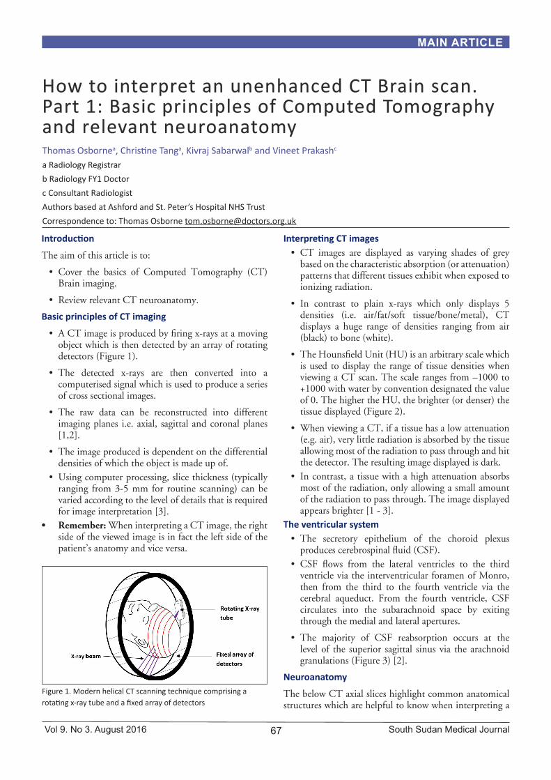
• A CT image is produced by firing x-rays at a moving object which is then detected by an array of rotating detectors (Figure 1).

• The detected x-rays are then converted into a computerised signal which is used to produce a series of cross sectional images.

• The raw data can be reconstructed into different imaging planes i.e. axial, sagittal and coronal planes [1,2].

• The image produced is dependent on the differential densities of which the object is made up of.

• Using computer processing, slice thickness (typically ranging from 3-5 mm for routine scanning) can be varied according to the level of details that is required for image interpretation [3].

• Remember: When interpreting a CT image, the right side of the viewed image is in fact the left side of the patient’s anatomy and vice versa.

Interpreting CT images • CT images are displayed as varying shades of grey

based on the characteristic absorption (or attenuation) patterns that different tissues exhibit when exposed to ionizing radiation.

• In contrast to plain x-rays which only displays 5 densities (i.e. air/fat/soft tissue/bone/metal), CT displays a huge range of densities ranging from air (black) to bone (white).

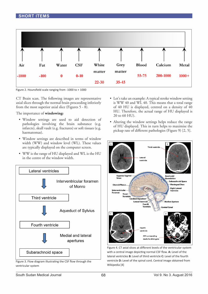
• The Hounsfield Unit (HU) is an arbitrary scale which is used to display the range of tissue densities when viewing a CT scan. The scale ranges from –1000 to +1000 with water by convention designated the value of 0. The higher the HU, the brighter (or denser) the tissue displayed (Figure 2).

• When viewing a CT, if a tissue has a low attenuation (e.g. air), very little radiation is absorbed by the tissue allowing most of the radiation to pass through and hit the detector. The resulting image displayed is dark.

• In contrast, a tissue with a high attenuation absorbs most of the radiation, only allowing a small amount of the radiation to pass through. The image displayed appears brighter [1 - 3].

The ventricular system• The secretory epithelium of the choroid plexus

produces cerebrospinal fluid (CSF). • CSF flows from the lateral ventricles to the third

ventricle via the interventricular foramen of Monro, then from the third to the fourth ventricle via the cerebral aqueduct. From the fourth ventricle, CSF circulates into the subarachnoid space by exiting through the medial and lateral apertures.

• The majority of CSF reabsorption occurs at the level of the superior sagittal sinus via the arachnoid granulations (Figure 3) [2].

Neuroanatomy

The below CT axial slices highlight common anatomical structures which are helpful to know when interpreting a

Figure 1. Modern helical CT scanning technique comprising a rotating x-ray tube and a fixed array of detectors

South Sudan Medical Journal Vol 9. No 3. August 2016 68

SHORT ITEMS

CT Brain scan. The following images are representative axial slices through the normal brain proceeding inferiorly from the most superior axial slice (Figures 5 - 8).

The importance of windowing:

• Window settings are used to aid detection of pathologies involving the brain substance (e.g. infarcts), skull vault (e.g. fractures) or soft tissues (e.g. haematomas).

• Window settings are described in terms of window width (WW) and window level (WL). These values are typically displayed on the computer screen.

• WW is the range of HU displayed and WL is the HU in the centre of the window width.

• Let’s take an example: A typical stroke window setting is WW 40 and WL 40. This means that a total range of 40 HU is displayed, centred on a density of 40 HU. Therefore, the actual range of HU displayed is 20 to 60 HU).

• Altering the window settings helps reduce the range of HU displayed. This in turn helps to maximise the pickup rate of different pathologies (Figure 9) [2, 5].

Figure 2. Hounsfield scale ranging from -1000 to + 1000

Figure 3. Flow diagram illustrating the CSF flow through the ventricular system

Figure 4. CT axial slices at different levels of the ventricular system with a central image depicting normal CSF flow. A: Level of the lateral ventricles B: Level of third ventricle C: Level of the fourth ventricle D: Level of the spinal cord. Central image obtained from Wikipedia [4]

Vol 9. No 3. August 2016 South Sudan Medical Journal 69

SHORT ITEMS

Figure 6. Axial CT slice at the level of the third ventricle [6]Figure 5. Axial CT slice at the level of the lateral ventricles [6]

Figure 8. Axial CT slice at the level of the pons [6].Figure 7. Axial CT slice at the level of the pituitary fossa [6].

Figure 9. Common window settings used when interpreting a normal CT Brain scan. A: Brain window (WW 80, WL 40); B: Bone window (WW 3000, WL 500); C: Soft tissue window (WW 260, WL 80); D: Stroke window (WW 40, WL 40).

References

1. Allisy-Roberts PJ, Williams J. Saunders Ltd.; 2 edition (25 Oct. 2007). Farr’s Physics for Medical Imaging.

2. Osborn AG. Amirsys, Inc; annotated edition edition (1 Dec. 2012). Osborn’s Brain: Imaging, Pathology, and Anatomy.

3. Osborn AG, Salzman KL, Jhaveri MD et al. AMIRSYS; 3 edition (25 Nov. 2015). Diagnostic Imaging: Brain.

4. Openstax College. Anatomy & Physiology, Connexions Web site. Created April 2013. https://commons.wikimedia.org/wiki/File:1317_CFS_Circulation.jpg (accessed 14May 2016).

5. Hacking C, Jones J et al. Radiopaedia. CT Head (an approach). http://radiopaedia.org/articles/ct-head-an-approach (accessed 14 May 2016).

6. Weir J, Abrahams PH, Spratt JD et al. Mosby; 4 edition (2 Mar. 2010). Imaging Atlas of Human Anatomy.

All CT images used in this article are the property of the Ashford and St. Peter’s Hospitals NHS Foundation Trust.