hp prime graphing calculator user guide
TRANSCRIPT

HP Prime Graphing Calculator User Guide

Edition1Part Number NW280-200X
Legal NoticesThis manual and any examples contained herein are provided "as is" and are subject to change without notice. Hewlett-Packard Company makes no warranty of any kind with regard to this manual, including, but not limited to, the implied warranties of merchantability, non-infringement and fitness for a particular purpose.
Hewlett-Packard Company shall not be liable for any errors or for incidental or consequential damages in connection with the furnishing, performance, or use of this manual or the exam-ples contained herein.
Product Regulatory & Environment InformationProduct Regulatory and Environment Information is provided on the CD shipped with this prod-uct.

Copyright © 2013 Hewlett-Packard Development Company, L.P.Reproduction, adaptation, or translation of this manual is prohibited without prior written per-mission of Hewlett-Packard Company, except as allowed under the copyright laws.
Printing HistoryEdition 1 May 2013


Contents 1
Contents
PrefaceManual conventions ................................................................ 9Notice ................................................................................. 10
1 Getting startedBefore starting ........................................................................ 9On/off, cancel operations...................................................... 10The display .......................................................................... 11
Sections of the display ...................................................... 12Navigation........................................................................... 14
Touch gestures ................................................................. 14The keyboard ....................................................................... 15
Context-sensitive menu ...................................................... 17Entry and edit keys................................................................ 17
Shift keys......................................................................... 19Adding text...................................................................... 20Math keys ....................................................................... 20
Menus ................................................................................. 25Toolbox menus................................................................. 26
Input forms ........................................................................... 26System-wide settings .............................................................. 27
Home settings .................................................................. 27Specifying a Home setting ................................................. 31
Mathematical calculations ...................................................... 32Choosing an entry type ..................................................... 33Entering expressions ......................................................... 34Reusing previous expressions and results ............................. 36Storing a value in a variable.............................................. 39
Complex numbers ................................................................. 40Sharing data ........................................................................ 40Online Help ......................................................................... 42
2 Reverse Polish Notation (RPN)History in RPN mode ............................................................. 44Sample calculations............................................................... 45Manipulating the stack........................................................... 47
3 Computer algebra system (CAS)CAS view............................................................................. 51
2 Contents
CAS calculations ...................................................................52Settings ................................................................................53
4 An introduction to HP appsApplication Library ................................................................61App views ............................................................................62
Symbolic view ..................................................................63Symbolic Setup view .........................................................64Plot view..........................................................................64Plot Setup view .................................................................65Numeric view...................................................................66Numeric Setup view ..........................................................68
Quick example......................................................................69Common operations in Symbolic view......................................71
Symbolic view: Summary of menu buttons............................76Common operations in Symbolic Setup view.............................76Common operations in Plot view .............................................77
Zoom ..............................................................................78Trace...............................................................................84Plot view: Summary of menu buttons....................................86
Common operations in Plot Setup view.....................................86Configure Plot view...........................................................86
Common operations in Numeric view ......................................90Zoom ..............................................................................90Evaluating........................................................................92Custom tables...................................................................93Numeric view: Summary of menu buttons.............................94
Common operations in Numeric Setup view..............................95Combining Plot and Numeric Views.........................................96Adding a note to an app........................................................96Creating an app....................................................................97App functions and variables ...................................................99
5 Function appGetting started with the Function app .....................................103Analyzing functions .............................................................109The Function Variables .........................................................114Summary of FCN operations.................................................116
6 Advanced Graphing appGetting started with the Advanced Graphing app ...............118
7 GeometryGetting started with the Geometry app...................................123

Contents 3
Plot view in detail................................................................ 129Plot Setup view............................................................... 134
Symbolic view in detail ........................................................ 136Symbolic Setup view....................................................... 138
Numeric view in detail......................................................... 138Geometric objects ............................................................... 141Geometric transformations ................................................... 148Geometry functions and commands....................................... 151
Symbolic view: Cmds menu ............................................. 152Numeric view: Cmds menu.............................................. 160Other Geometry functions................................................ 164
8 SpreadsheetGetting started with the Spreadsheet app............................... 171Basic operations ................................................................. 175
Navigation, selection and gestures ................................... 175Cell references ............................................................... 176Cell naming................................................................... 176Entering content ............................................................. 177Copy and paste ............................................................. 180
External references .............................................................. 180Referencing variables...................................................... 181
Buttons and keys ................................................................. 183Formatting options .............................................................. 184Spreadsheet functions.......................................................... 186
9 Statistics 1Var appGetting started with the Statistics 1Var app ............................ 187Entering and editing statistical data....................................... 191Computed statistics.............................................................. 194Plotting .............................................................................. 195
Plot types....................................................................... 196Setting up the plot (Plot Setup view) .................................. 197Exploring the graph ........................................................ 197
10 Statistics 2Var appGetting started with the Statistics 2Var app ............................ 199Entering and editing statistical data....................................... 204
Numeric view menu items................................................ 205Defining a regression model................................................. 206Computed statistics.............................................................. 208Plotting statistical data ......................................................... 210
Plot view: menu items...................................................... 211
4 Contents
Plot setup .......................................................................211Predicting values.............................................................212Troubleshooting a plot .....................................................213
11 Inference appGetting started with the Inference app....................................215Importing statistics ...............................................................219Hypothesis tests ...................................................................221
One-Sample Z-Test ..........................................................222Two-Sample Z-Test ..........................................................223One-Proportion Z-Test ......................................................224Two-Proportion Z-Test ......................................................225One-Sample T-Test ..........................................................227Two-Sample T-Test ...........................................................228
Confidence intervals ............................................................229One-Sample Z-Interval .....................................................229Two-Sample Z-Interval......................................................230One-Proportion Z-Interval .................................................231Two-Proportion Z-Interval..................................................232One-Sample T-Interval......................................................232Two-Sample T-Interval ......................................................233
12 Solve appGetting started with the Solve app .........................................235
One equation.................................................................235Several equations ...........................................................239Limitations......................................................................240
Solution information.............................................................240
13 Linear Solver appGetting started with the Linear Solver app...............................243Menu items.........................................................................245
14 Parametric appGetting started with the Parametric app..................................247
15 Polar appGetting started with the Polar app .........................................253
16 Sequence appGetting started with the Sequence app ...................................257Another example: A table of cubes ........................................261
17 Finance app
Contents 5
Getting Started with the Finance app..................................... 263Cash flow diagrams ............................................................ 265Time value of money (TVM) .................................................. 266TVM calculations: Another example....................................... 267Calculating amortizations..................................................... 268
18 Triangle Solver appGetting started with the Triangle Solver app ........................... 271Choosing triangle types ....................................................... 273Special cases ..................................................................... 273
19 The Explorer appsLinear Explorer app............................................................. 275Quadratic Explorer app....................................................... 277Trig Explorer app................................................................ 280
20 Functions and commandsKeyboard functions ............................................................. 285Math menu......................................................................... 288
Numbers ....................................................................... 288Arithmetic...................................................................... 289Trigonometry.................................................................. 291Hyperbolic .................................................................... 292Probability ..................................................................... 292List................................................................................ 297Matrix........................................................................... 297Special ......................................................................... 297
CAS menu.......................................................................... 298Algebra ........................................................................ 299Calculus ........................................................................ 299Solve ............................................................................ 302Rewrite.......................................................................... 304Integer .......................................................................... 306Polynomial..................................................................... 307Plot ............................................................................... 311
App menu .......................................................................... 312Function app functions .................................................... 312Solve app functions ........................................................ 313Spreadsheet functions ..................................................... 314Statistics 1Var app functions ............................................ 330Statistics 2Var app functions ............................................ 331Inference app functions ................................................... 332Finance app functions ..................................................... 333

6 Contents
Linear Solver app functions ..............................................334Triangle Solver app functions ...........................................335Linear Explorer functions ..................................................336Quadratic Explorer functions ............................................336Geometry app function....................................................337Common app functions....................................................337
Ctlg menu...........................................................................338Creating your own functions .................................................371
21 VariablesHome variables...................................................................377App variables .....................................................................378
Function app variables ....................................................378Geometry app variables ..................................................379Spreadsheet app variables...............................................379Advanced Graphing app variables ...................................380Solve app variables ........................................................380Statistics 1Var app variables ............................................381Statistics 2Var app variables ............................................383Inference app variables ...................................................385Parametric app variables .................................................387Polar app variables.........................................................387Finance app variables .....................................................388Linear Solver app variables..............................................388Triangle Solver app variables ...........................................389Linear Explorer app variables...........................................389Quadratic Explorer app variables .....................................389Trig Explorer app variables ..............................................389Sequence app variables ..................................................390
22 Units and constantsUnits ..................................................................................391Unit calculations ..................................................................392Unit tools ............................................................................394Physical constants ................................................................395
List of constants...............................................................396
23 ListsCreate a list in the List Catalog..............................................399
The List Editor .................................................................401Deleting lists .......................................................................403Lists in Home view ...............................................................403List functions........................................................................405

Contents 7
Finding statistical values for lists ............................................ 408
24 MatricesCreating and storing matrices............................................... 412Working with matrices......................................................... 413Matrix arithmetic................................................................. 416Solving systems of linear equations ....................................... 419Matrix functions and commands............................................ 421Matrix functions .................................................................. 422
Examples....................................................................... 426
25 Notes and InfoThe Note Catalog ............................................................... 429The Note Editor .................................................................. 430
26 ProgrammingThe Program Catalog .......................................................... 438Creating a new program ..................................................... 441
The Program Editor ......................................................... 441The HP Prime programming language ................................... 450
The User Keyboard: Customizing key presses .................... 455App programs ............................................................... 459
Program commands ............................................................ 464Commands under the Tmplt menu..................................... 465Block ............................................................................ 465Branch .......................................................................... 465Loop ............................................................................. 466Variable ........................................................................ 470Function ........................................................................ 470Commands under the Cmds menu .................................... 470Strings .......................................................................... 470Drawing........................................................................ 473Matrix........................................................................... 480App Functions ................................................................ 482Integer .......................................................................... 483I/O .............................................................................. 485More ............................................................................ 489Variables and Programs .................................................. 492
27 Integer arithmeticThe default base ................................................................. 514
Changing the default base............................................... 515Examples of integer arithmetic .............................................. 516Integer manipulation............................................................ 517

8 Contents
Base functions .....................................................................518
28 Limiting functionalityExam configurations ............................................................519
Modifying the default configuration...................................520Creating a new configuration...........................................521
Activating Exam Mode.........................................................522Cancelling exam mode....................................................524
Modifying configurations......................................................524To change a configuration ...............................................524Deleting configurations ....................................................524
A GlossaryB Troubleshooting
Calculator not responding ....................................................531To reset .........................................................................531To restore factory settings.................................................531If the calculator does not turn on .......................................531
Operating limits ..................................................................532Status messages ..................................................................532
C Product Regulatory InformationFederal Communications Commission Notice..........................535European Union Regulatory Notice........................................537
Index ...................................................................................541

Preface 9
Preface
Manual conventionsThe following conventions are used in this manual to represent the keys that you press and the menu options that you choose to perform operations.
• A key that initiates an unshifted function is represented by an image of that key:
e,B,H, etc.
• A key combination that initiates a shifted unction (or inserts a character) is represented by the appropriate shift key (S or A) followed by the key for that function or character:
Sh initiates the natural exponential function and Az inserts the pound character (#)
The name of the shifted function may also be given in parentheses after the key combination:
SJ(Clear), SY (Setup)
• A key pressed to insert a digit is represented by that digit:
5, 7, 8, etc.
• All fixed on-screen text—such as screen and field names—appear in bold:
CAS Settings, XSTEP, Decimal Mark, etc.
• A menu item selected by touching the screen is represented by an image of that item:
, , .
Note that you must use your finger to select a menu item. Using a stylus or something similar will not select whatever is touched.

10 Preface
• Items you can select from a list, and characters on the entry line, are set in a non-proportional font, as follows:
Function, Polar, Parametric, Ans, etc.
• Cursor keys are represented by =, \, >, and <. You use these keys to move from field to field on a screen, or from one option to another in a list of options.
• Error messages are enclosed inverted commas:
“Syntax Error”
NoticeThis manual and any examples contained herein are provided as-is and are subject to change without notice. Except to the extent prohibited by law, Hewlett-Packard Company makes no express or implied warranty of any kind with regard to this manual and specifically disclaims the implied warranties and conditions of merchantability and fitness for a particular purpose and Hewlett-Packard Company shall not be liable for any errors or for incidental or consequential damage in connection with the furnishing, performance or use of this manual and the examples herein.
1994–1995, 1999–2000, 2003–2006, 2010–2013 Hewlett-Packard Development Company, L.P.
The programs that control your HP Prime are copyrighted and all rights are reserved. Reproduction, adaptation, or translation of those programs without prior written permission from Hewlett-Packard Company is also prohibited.
For hardware warranty information, please refer to the HP Prime Quick Start Guide.
Product Regulatory and Environment Information is provided on the CD shipped with this product.

Getting started 9
1
Getting started
The HP Prime Graphing Calculator is an easy-to-use yet powerful graphing calculator designed for secondary mathematics education and beyond. It offers hundreds of functions and commands, and includes a computer algebra system (CAS) for symbolic calculations.
In addition to an extensive library of functions and commands, the calculator comes with a set of HP apps. A HP app is a special application designed to help you explore a particular branch of mathematics or to solve a problems of a particular type. For example, there is a HP app that will help you explore geometry and another to help you explore parametric equations. There are also apps to help you solve systems of linear equations and to solve time-value-of-money problems.
The HP Prime also has its own programming language you can use to explore and solve mathematical problems.
Functions, commands, apps and programming are covered in detail later in this guide. In this chapter, the general features of the calculator are explained, along with common interactions and basic mathematical operations.
Before startingCharge the battery fully before using the calculator for the first time. To charge the battery, either:
• Connect the calculator to a computer using the USB cable that came in the package with your HP Prime. (The PC needs to be on for charging to occur.)
• Connect the calculator to a wall outlet using the HP-provided wall adapter.

10 Getting started
When the calculator is on, a battery symbol appears in the title bar of the screen. Its appearance will indicate how much power the battery has. A flat battery will take approximately 4 hours to become fully charged.
Battery Warning • To reduce the risk of fire or burns, do not disassemble, crush or puncture the battery; do not short the external contacts; and do not dispose of the battery in fire or water.
• To reduce potential safety risks, only use the battery provided with the calculator, a replacement battery provided by HP, or a compatible battery recommended by HP.
• Keep the battery away from children.
• If you encounter problems when charging the calculator, stop charging and contact HP immediately.
Adapter Warning • To reduce the risk of electric shock or damage to equipment, only plug the AC adapter into an AC outlet that is easily accessible at all times.
• To reduce potential safety risks, only use the AC adapter provided with the calculator, a replacement AC adapter provided by HP, or an AC adapter purchased as an accessory from HP.
On/off, cancel operationsTo turn on Press O to turn on the calculator.
To cancel When the calculator is on, pressing the J key cancels the current operation. For example, it will clear whatever you have entered on the entry line. It will also close a menu and a screen.
To turn off Press SO(Off) turn the calculator off.
To save power, the calculator turns itself off after several minutes of inactivity. All stored and displayed information is saved.
Getting started 11
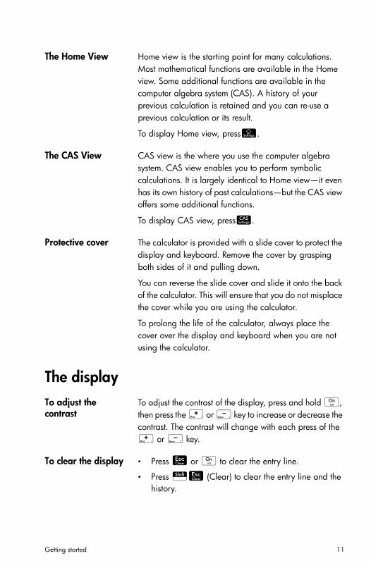
The Home View Home view is the starting point for many calculations. Most mathematical functions are available in the Home view. Some additional functions are available in the computer algebra system (CAS). A history of your previous calculation is retained and you can re-use a previous calculation or its result.
To display Home view, pressH.
The CAS View CAS view is the where you use the computer algebra system. CAS view enables you to perform symbolic calculations. It is largely identical to Home view—it even has its own history of past calculations—but the CAS view offers some additional functions.
To display CAS view, pressK.
Protective cover The calculator is provided with a slide cover to protect the display and keyboard. Remove the cover by grasping both sides of it and pulling down.
You can reverse the slide cover and slide it onto the back of the calculator. This will ensure that you do not misplace the cover while you are using the calculator.
To prolong the life of the calculator, always place the cover over the display and keyboard when you are not using the calculator.
The displayTo adjust the contrast
To adjust the contrast of the display, press and hold O, then press the + or w key to increase or decrease the contrast. The contrast will change with each press of the + or w key.
To clear the display • Press J or O to clear the entry line.
• Press SJ (Clear) to clear the entry line and the history.

12 Getting started
Sections of the display
Home view has four sections (shown above). The title bar shows either the screen name or the name of the app you are currently using—Function in the example above. It also shows the time, a battery power indicator, and a number of symbols that indicate various calculator settings. These are explained below. The history displays a record of your past calculations. The entry line displays the object you are currently entering or modifying. The object could be a parameter, expression, list, matrix, line of programming code, etc. The menu buttons are options that are relevant to the current display. These options are selected by tapping the corresponding menu button. (Only a labeled button has a function.) You close a menu without making a selection from it by pressing J.
Annunciators. Annunciators are symbols or characters that appear in the title bar. They indicate that certain settings are current, and also provide time and battery power information.
Title bar
History
Menu buttonsEntry line
Annunciator Meaning
[Lime green] The angle mode setting is currently degrees.
[Lime green] The angle mode setting is currently radians.
π
Getting started 13
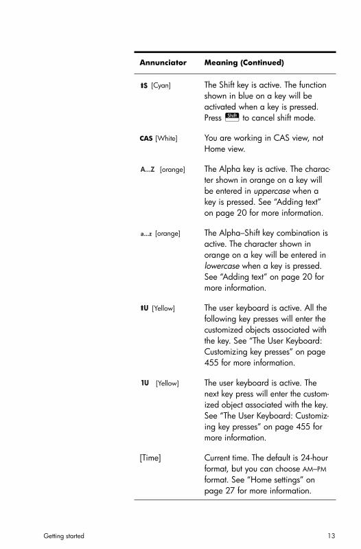
[Cyan] The Shift key is active. The function shown in blue on a key will be activated when a key is pressed. Press S to cancel shift mode.
CAS [White] You are working in CAS view, not Home view.
[orange] The Alpha key is active. The charac-ter shown in orange on a key will be entered in uppercase when a key is pressed. See “Adding text” on page 20 for more information.
[orange] The Alpha–Shift key combination is active. The character shown in orange on a key will be entered in lowercase when a key is pressed. See “Adding text” on page 20 for more information.
[Yellow] The user keyboard is active. All the following key presses will enter the customized objects associated with the key. See “The User Keyboard: Customizing key presses” on page 455 for more information.
[Yellow] The user keyboard is active. The next key press will enter the custom-ized object associated with the key. See “The User Keyboard: Customiz-ing key presses” on page 455 for more information.
[Time] Current time. The default is 24-hour format, but you can choose AM–PM format. See “Home settings” on page 27 for more information.
Annunciator Meaning (Continued)
SS
A...Z
a...z
UU
1U1U

14 Getting started
NavigationThe HP Prime offers two modes of navigation: touch and keys. In many cases, you can tap on an icon, field, menu, or object to select (or deselect) it. For example, you can open the Function app by tapping once on its icon in the Application Library. However, to open the Application Library, you will need to press a key: I.
Selections can often be made either by tapping or by using the keys. For instance, as well as tapping an icon in the Application Library, you can also press the cursor keys—=,\,<,>—until the app you want to open is highlighted, and then press E. In the Application Library, you can also type the first one or two letters of an app’s name to highlight the app. Then either tap the app’s icon or press E to open it.
Sometimes a touch or key–touch combination is available. For example, you can deselect a toggle option either by tapping twice on it, or by using the arrow keys to move to the field and then tapping a touch button along the bottom of the screen (in this case ).
Note that you must use your finger to select an item by touch. Using a stylus or something similar will not select whatever is touched.
Touch gesturesIn addition to selection by tapping, there are other touch-related operations available to you:
To quickly move from page to page, flick:
Place a finger on the screen and quickly swipe it in the desired direction (up or down).
Battery-charge indicator.
Annunciator Meaning (Continued)

Getting started 15
To pan, drag your finger horizontally or vertically across the screen.
To quickly zoom in, make an open pinch:
Place the thumb and a finger close together on the screen and move them apart. Only lift them from the screen when you reach the desired magnification.
To quickly zoom out, make an closed pinch:
Place the thumb and a finger some distance apart on the screen and move them toward each other. Only lift them from the screen when you reach the desired magnification.
Note that pinching to zoom only works in applications that feature zooming (such as where graphs are plotted). In other applications, pinching will do nothing, or do something other than zooming. For example, in the Spreadsheet app, pinching will change the width of a column or the height of a row.
The keyboardThe numbers in the legend below refer to the parts of the keyboard described in the illustration below the legend.
Number Feature
1 LCD and touch-screen: 320 × 240 pixels
2 Context-sensitive touch-button menu
3 HP Apps keys
4 Home view and preference settings
5 Common math and science functions
6 Alpha and Shift keys
7 On, Cancel and Off key
8 List, matrix, program, and note catalogs
9 Last Answer key (Ans)
10 Enter key
11 Backspace and Delete key

16 Getting started
12 Menu (and Paste) key
13 CAS (and CAS preferences) key
14 View (and Copy) key
15 Escape (and Clear) key
16 Help key
17 Rocker wheel (for cursor movement)
Number Feature
1
2
3
4
5
6
7
8
9
11
1314
12
1516
10
17
Getting started 17
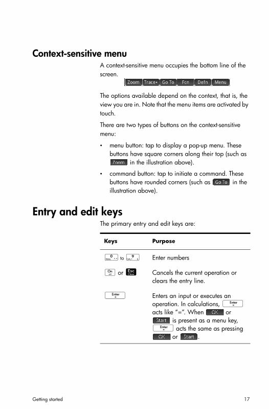
Context-sensitive menu A context-sensitive menu occupies the bottom line of the screen.
The options available depend on the context, that is, the view you are in. Note that the menu items are activated by touch.
There are two types of buttons on the context-sensitive menu:
• menu button: tap to display a pop-up menu. These buttons have square corners along their top (such as
in the illustration above).
• command button: tap to initiate a command. These buttons have rounded corners (such as in the illustration above).
Entry and edit keysThe primary entry and edit keys are:
Keys Purpose
N to r Enter numbers
O or J Cancels the current operation or clears the entry line.
E Enters an input or executes an operation. In calculations, E acts like “=”. When or
is present as a menu key, E acts the same as pressing
or .

18 Getting started
Q For entering a negative number. For example, to enter –25, press Q25. Note: this is not the same operation that is performed by the subtraction key (w).
F Math template: Displays a palette of pre-formatted templates repre-senting common arithmetic expres-sions.
d Enters the independent variable (that is, either X, T, or N, depend-ing on the app that is current).
Sv Relations palette: Displays a palette of comparison operators and Bool-ean operators.
Sr Special symbols palette: Displays a palette of common math and Greek characters.
Sc Automatically inserts the degree, minute, or second symbol accord-ing to the context.
C Backspace. Deletes the character to the left of the cursor. It will also return the highlighted field to its default value, if it has one.
SC Delete. Deletes the character to the right of the cursor.
SJ(Clear) Clears all data on the screen (including the history). On a set-tings screen—for example Plot Setup—returns all settings to their default values.
Keys Purpose (Continued)

Getting started 19
Shift keysThere are two shift keys that you use to access the operations and characters printed on the bottom of the keys: S and A.
<>=\ Cursor keys: Moves the cursor around the display. Press S\ to move to the end of a menu or screen, or S= to move to the start.
Sa Displays all the available characters. To enter a character, use the cursor keys to highlight it, and then tap . To select multiple characters, select one, tap , and continue likewise before pressing . There are many pages of characters. You can jump to a particular Unicode block by tapping and selecting the block. You can also flick from page to page.
Keys Purpose (Continued)
Key Purpose
S Press S to access the operations printed in blue on a key. For instance, to access the settings for Home view, press SH.
A Press the A key to access the characters printed in orange on a key. For instance, to type Z, press A and then press y. For a lowercase letter, press AS and then the letter. To type more than one letter, press A a second time to lock the alpha shift.
20 Getting started
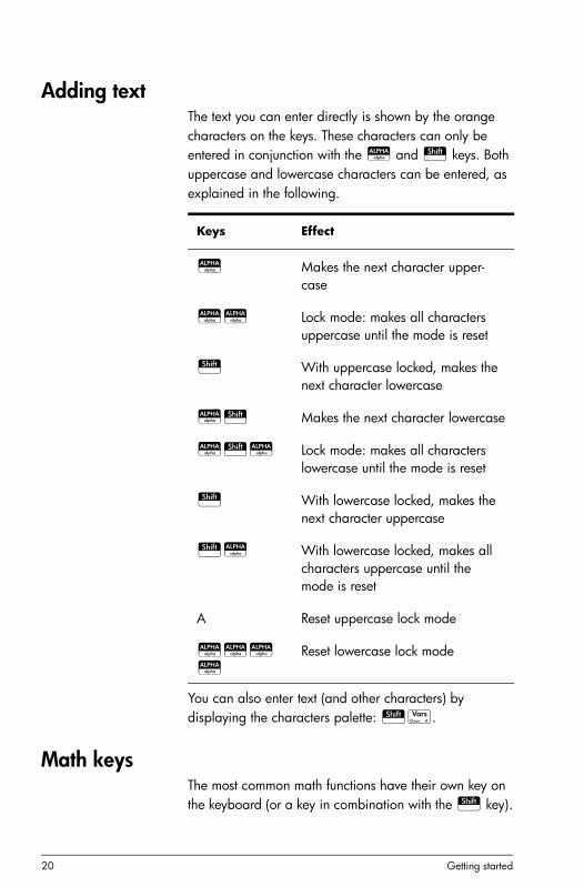
Adding textThe text you can enter directly is shown by the orange characters on the keys. These characters can only be entered in conjunction with the A and S keys. Both uppercase and lowercase characters can be entered, as explained in the following.
You can also enter text (and other characters) by displaying the characters palette: Sa.
Math keysThe most common math functions have their own key on the keyboard (or a key in combination with the S key).
Keys Effect
A Makes the next character upper-case
AA Lock mode: makes all characters uppercase until the mode is reset
S With uppercase locked, makes the next character lowercase
AS Makes the next character lowercase
ASA Lock mode: makes all characters lowercase until the mode is reset
S With lowercase locked, makes the next character uppercase
SA With lowercase locked, makes all characters uppercase until the mode is reset
A Reset uppercase lock mode
AAAA
Reset lowercase lock mode

Getting started 21
Example 1: To calculate SIN(10), press e10 and press E. The answer displayed is –0,544… (if your angle measure setting is radians).
Example 2: To find the square root of 256, press Sj 256 and press E. The answer displayed is 16. Notice that the S key initiates the operator represented in blue on the next key pressed (in this case √ on the j key).
The mathematical functions not represented on the keyboard are on the Math, CAS, and Catlg menus (see chapter 20, “Functions and commands”, starting on page 283).
Note that the order in which you enter operands and operators is determined by the entry mode. By default, the entry mode is textbook, which means that you enter operands and operators just as you would if you were writing the expression on paper. If your preferred entry mode is Reverse Polish Notation, the order of entry is different. (See chapter 2, “Reverse Polish Notation (RPN)”, starting on page 43.)
Math template
The math template key (F) helps you insert the framework for common calculations (and for vectors, matrices, and hexagesimal numbers). It displays a palette of pre-formatted outlines to which you add the constants, variables, and so on. Just tap on the template you want (or use the arrow keys to highlight it and press E). Then enter the components needed to complete the calculation.
Example: Suppose you want to find the cube root of 945:
1. In Home view, press F.
2. Select .
The skeleton or framework for your calculation now appears on the entry line:
3. Each box on the template needs to be completed:

22 Getting started
3>945
4. Press E to display the result: 9.813…
The template palette can save you a lot of time, especially with calculus calculations.
You can display the palette at any stage in defining an expression. In other words, you don’t need to start out with a template. Rather, you can embed one or more templates at any point in the definition of an expression.
Math shortcuts
As well as the math template, there are other similar screens that offer a palette of math characters. For example, pressing Sr displays the special symbols palette, shown at the right. Select a character by tapping it (or scrolling to it and pressing E).
A similar palette—the relations palette—is displayed if you press Sr. The palette displays operators useful in math and programming. Again, just tap the character you want.
Other math shortcut keys include d. Pressing this key inserts an X, T, , or N depending on what app you are using. (This is explained further in the chapters describing the apps.)
Similarly, pressing Sc enters a degree, minute, or second character. It enters ° if no degree symbol is part of your expression; enters ′ if the previous entry is a value in degrees; and enters ″ if the previous entry is a value in minutes. Thus entering:
36Sc40Sc20Sc
yields 36°40′20″. See “Hexagesimal numbers” on page 23 for more information.
Fractions The fraction key (c) cycles through thee varieties of fractional display. If the current answer is the decimal

Getting started 23
fraction 5.25, pressing c converts the answer to the vulgar fraction 21/4. If you press c again, the answer is converted to a mixed number fraction (5 + 1/4). If pressed again, the display returns to the decimal fraction (5.25).
The HP Prime will approximate fraction and mixed number representations in cases where it cannot find exact ones. For example, enter to see the decimal approximation: 2.236…. Press c once to see and again to see
. Pressing c a third time will cycle back to the original decimal representation.
Hexagesimal numbers
Any decimal result can de displayed in hexagesimal format; that is, in units subdivided into groups of 60. This includes degrees, minutes, and seconds as well as hours, minutes, and seconds. For example, enter to see the decimal result: 1.375. Now press S c to see 1°22′30″ . Press S c again to return to the decimal representation.
The HP Prime will produce the best approximation in cases where an exact result is not possible. Enter to see the decimal approximation: 2.236… Press S c to see 2°14′9.844719″ .
Note that the degree and minute entries must be positive integers. Decimals are not allowed, except in the seconds.
Note too that the HP Prime treats a value in hexgesimal format as a single entity. Hence any operation performed on a hexagesimal value is performed on the entire value. For example, if
5
930249416020------------------
298209416020------------------+
118------
5

24 Getting started
you enter 10°25′26″ 2, the whole value is squared, not just the seconds component. The result in this case is 108°39′26.854445″ .
EEX key (powers of 10)
Numbers like and are expressed in scientific notation, that is, in terms of powers of ten. This is simpler to work with than 50 000 or 0.000 000321. To enter numbers like these, use the B functionality. This is easier than using s10k.
Example: Suppose you want to calculate
First select Scientific as the number format.
1. Open the Home Settings window.
SH
2. Select Scientific from the Number Format menu.
3. Return home: H
4. Enter 4BQ13 s6B23n 3BQ5
5. Press E
The result is 8.0000E15. This is equivalent to 8 × 10¹⁵.
5 104 3.21 10
7–
4 1013– 6 10
23
3 105–
----------------------------------------------------

Getting started 25
MenusA menu offers you a choice of items. As in the case shown at the right, some menus have sub-menus and sub-sub-menus.
To select from a menu
There are two techniques for selecting an item from a menu:
• direct tapping and
• using the arrow keys to highlight the item you want and then either tapping or pressing E.
Note that the menu of buttons along the bottom of the screen can only be activated by tapping.
Shortcuts • Press = when you are at the top of the menu to immediately display the last item in the menu.
• Press \ when you are at the bottom of the menu to immediately display the first item in the menu.
• Press S\ to jump straight to the bottom of the menu.
• Press S= to jump straight to the top of the menu.
• Enter the first few characters of the item’s name to jump straight to that item.
• Enter the number of the item shown in the menu to jump straight to that item.
To close a menu A menu will close automatically when you select an item from it. If you want to close a menu without selecting anything from it, use one of the following techniques:
• To close the last opened menu or sub-menu, press O.
• To close all open menus, press J.

26 Getting started
Toolbox menusThe Toolbox menus (D) are a collection of menus offering functions and commands useful in mathematics and programming. The Math, CAS, and Catlg menus offer over 400 functions and commands. The items on these menus are described in detail in chapter 20, “Functions and commands”, starting on page 283).
Input formsAn input form is a screen that provides one or more fields for you to enter data or select an option. It is another name for a dialog box.
• If a field allows you to enter data of your choice, you can select it, add your data, and tap . (There is no need to tap first.)
• If a field allows you to choose an item from a menu, you can tap on it (the field or the label for the field), tap on it again to display the options, and tap on the item you want. (You can also choose an item from an open list by pressing the cursor keys and pressing E when the option you want is highlighted.)
• If a field is a toggle field—one that is either selected or not selected—tap on it to select the field and tap on it again to select the alternate option. (Alternatively, select the field and tap .)
The illustration at the right shows an input form with all three types of field. Calculator Name is a free-form data-entry field, Font Size provides a menu of options, and Textbook Display is a toggle field.

Getting started 27
Reset input form fields
To reset a field to its default value, highlight the field and press C. To reset all fields to their default values, press SJ (Clear).
System-wide settingsSystem-wide settings are values that determine the appearance of windows, the format of numbers, the scale of plots, the units used by default in calculations, and much more.
There are two system-wide settings: Home settings and CAS settings. Home settings control Home view and the apps. CAS settings control how calculations are done in the computer algebra system. CAS settings are discussed in chapter 3.
Although Home settings control the apps, you can override certain Home settings once inside an app. For example, you can set the angle measure to radians in the Home settings but choose degrees as the angle measure once inside the Polar app. Degrees then remains the angle measure until you open another app that has a different angle measure.
Home settingsYou use the Home Settings input form to specify the settings for Home view (and the default settings for the apps). Press SH (Settings) to open the Home Settings input form. There are four pages of settings.

28 Getting started
Page 1
Setting Options
Angle Measure Degrees: 360 degrees in a circle.Radians: 2 radians in a circle.
The angle mode you set is the angle setting used in both Home view and the current app. This is to ensure that trigonometric calculations done in the current app and Home view give the same result.
Number Format
The number format you set is the for-mat used in all Home view calcula-tions.
Standard: Full-precision display.
Fixed: Displays results rounded to a number of decimal places. If you choose this option, a new field appears for you to enter the number of decimal places. For example, 123.456789 becomes 123.46 in Fixed 2 format.
Scientific: Displays results with an exponent one digit to the left of the decimal point, and the specified number of decimal places. For example, 123.456789 becomes 1.23E2 in Scientific 2 format.
Engineering: Displays results with an exponent that is a multiple of 3, and the specified number of significant digits beyond the first one. Example: 123.456E7 becomes 1.23E9 in Engineer-ing 2 format.
Getting started 29
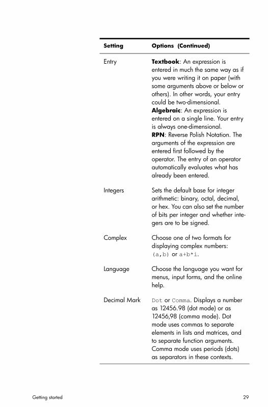
Entry Textbook: An expression is entered in much the same way as if you were writing it on paper (with some arguments above or below or others). In other words, your entry could be two-dimensional.Algebraic: An expression is entered on a single line. Your entry is always one-dimensional. RPN: Reverse Polish Notation. The arguments of the expression are entered first followed by the operator. The entry of an operator automatically evaluates what has already been entered.
Integers Sets the default base for integer arithmetic: binary, octal, decimal, or hex. You can also set the number of bits per integer and whether inte-gers are to be signed.
Complex Choose one of two formats for displaying complex numbers: (a,b) or a+b*i.
Language Choose the language you want for menus, input forms, and the online help.
Decimal Mark Dot or Comma. Displays a number as 12456.98 (dot mode) or as 12456,98 (comma mode). Dot mode uses commas to separate elements in lists and matrices, and to separate function arguments. Comma mode uses periods (dots) as separators in these contexts.
Setting Options (Continued)

30 Getting started
Page 2
Setting Options
Font Size Choose between small, medium, and large font for general display.
Calculator Name
Enter a name for the calculator.
Textbook Display
If selected, expressions and results are displayed in textbook format (that is, much as you would see in textbooks). If not selected, expres-sions and results are displayed in algebraic format (that is, in one-dimensional format). For example,
is displayed as [[4,5],[6,2]] in algebraic format.
Menu Display This setting determines whether the commands on the Math and CAS menus are presented descriptively or in common mathematical shorthand. The default is to provide the descriptive names for the functions. If you prefer the functions to be presented in mathematical shorthand, deselect this option.
Time Set the time and choose a format: 24-hour or AM–PM format.
Date Set the date and choose a format: YYYY/MM/DD, DD/MM/YYYY, or MM/DD/YYYY.
Color Theme Light: black text on a light back-groundDark: white text on a dark back-ground
4 56 2

Getting started 31
Page 3 Page 3 of the Home Settings input form is for setting Exam mode. This mode enables certain functions of the calculator to be disabled for a set period, with the disabling controlled by a password. This feature will primarily be of interest to those who supervise examinations and who need to ensure that the calculator is used appropriately by students sitting an examination. It is described in detail in chapter 28, “Limiting functionality”, starting on page 519.
Page 4 Page 4 of the Home Settings input form is for configuring your HP Prime to work on a wireless network. Visit www.hp.com/support for further information.
Specifying a Home settingThis example demonstrates how to change the number format from the default setting—Standard—to Scientific with two decimal places.
1. Press SH (Settings) to open the Home Settings input form.
The Angle Measure field is highlighted.
2. Tap on Number Format (either the field label or the field). This selects the field. (You could also have pressed \ to select it.)
Appearance Choose a color for the shading (such as the color of the highlight).
Setting Options (Continued)
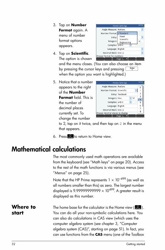
32 Getting started
3. Tap on Number Format again. A menu of number format options appears.
4. Tap on Scientific. The option is chosen and the menu closes. (You can also choose an item by pressing the cursor keys and pressing E when the option you want is highlighted.)
5. Notice that a number appears to the right of the Number Format field. This is the number of decimal places currently set. To change the number to 2, tap on it twice, and then tap on 2 in the menu that appears.
6. PressHto return to Home view.
Mathematical calculationsThe most commonly used math operations are available from the keyboard (see “Math keys” on page 20). Access to the rest of the math functions is via various menus (see “Menus” on page 25).
Note that the HP Prime represents 1 × 10–499 (as well as all numbers smaller than this) as zero. The largest number displayed is 9.99999999999 × 10499. A greater result is displayed as this number.
Where to start
The home base for the calculator is the Home view (H). You can do all your non-symbolic calculations here. You can also do calculations in CAS view (which uses the computer algebra system (see chapter 3, “Computer algebra system (CAS)”, starting on page 51). In fact, you can use functions from the CAS menu (one of the Toolbox

Getting started 33
menus) in an expression you are entering in Home view, and use functions from the Math menu (another of the Toolbox menus) in an expression you are entering in CAS view.
Choosing an entry typeThe first choice you need to make is the style of entry. The three types are:
• Textbook
An expression is entered in much the same way as if you were writing it on paper (with some arguments above or below or others). In other words, your entry could be two-dimensional, as in the example above.
• Algebraic
An expression is entered on a single line. Your entry is always one-dimensional.
• Advanced RPN (where RPN stands for Reverse Polish Notation). [Not available in CAS view.]
The arguments of the depression are entered first followed by the operator. The entry of an operator automatically evaluates what has already been entered. Thus you will need to enter a two-operator expression (as in the example above) in two steps, one for each operator:
Step 1: 5 h – the natural logarithm of 5 is calculated and displayed in history.
Step 2: Szn – is entered as a divisor and applied to the previous result.
More information about RPN mode can be found in chapter 2, “Reverse Polish Notation (RPN)”, starting on page 43.
Note that on page 2 of the Home Settings screen, you can specify whether you want to display your calculations

34 Getting started
in Textbook format or not. This refers to the appearance of your calculations in the history section of both Home view and CAS view. This is a different setting to the Entry setting discussed above.
Entering expressionsThe examples that follow assume that the entry mode is Textbook.
• An expression can contain numbers, functions, and variables.
• To enter a function, press the appropriate key, or open a Toolbox menu and select the function. You can also enter a function by using the alpha keys to spell out its name.
• When you have finished entering the expression, press E to evaluate it.
If you make a mistake while entering an expression, you can:
• delete the character to the left of the cursor by pressing C
• delete the character to the right of the cursor by pressing SC
• clear the entire entry line by pressing O or J.
Example Calculate
R23jw14Sk8>>nQ3>h45E
This example illustrates a number of important points to be aware of:
• the importance of delimiters (such as parentheses)
• how to enter negative numbers
• the use of implied versus explicit multiplication.
232
14 8–3–
---------------------------- 45 ln
Getting started 35
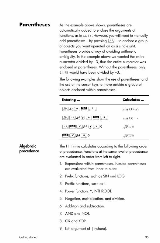
Parentheses As the example above shows, parentheses are automatically added to enclose the arguments of functions, as in LN(). However, you will need to manually add parentheses—by pressing R—to enclose a group of objects you want operated on as a single unit. Parentheses provide a way of avoiding arithmetic ambiguity. In the example above we wanted the entire numerator divided by –3, thus the entire numerator was enclosed in parentheses. Without the parentheses, only 14√8 would have been divided by –3.
The following examples show the use of parentheses, and the use of the cursor keys to move outside a group of objects enclosed within parentheses.
Algebraic precedence
The HP Prime calculates according to the following order of precedence. Functions at the same level of precedence are evaluated in order from left to right.
1. Expressions within parentheses. Nested parentheses are evaluated from inner to outer.
2. Prefix functions, such as SIN and LOG.
3. Postfix functions, such as !
4. Power function, ^, NTHROOT.
5. Negation, multiplication, and division.
6. Addition and subtraction.
7. AND and NOT.
8. OR and XOR.
9. Left argument of | (where).
Entering ... Calculates …
e45+Sz
eR45>+Sz
RSj85>s9
Sj85s9
45 + sin
45 sin +
85 9
85 9

36 Getting started
10. Equals (=).
Negative numbers
It is best to press Q to start a negative number or to insert a negative sign. Pressing w instead will, in some situations, be interpreted as an operation to subtract the next number you enter from the last result. (This is explained in “To reuse the last result” on page 37.)
To raise a negative number to a power, enclose it in parentheses. For example, (–5)2 = 25, whereas –52 = –25.
Explicit and implied multiplication
Implied multiplication takes place when two operands appear with no operator between them. If you enter AB, for example, the result is A*B. Notice in the example on page 34 that we entered 14Sk8 without the multiplication operator after 14. For the sake of clarity, the calculator adds the operator to the expression in history, but it is not strictly necessary when you are entering the expression. You can, though, enter the operator if you wish (as was done in the examples on page 35). The result will be the same.
Large results If the result of a calculation is too long to fit on the display line in history, you can press > to scroll the display to the right. Pressing < scrolls the display to the left.
If the result is too tall to be seen in its entirety—for example, a many-rowed matrix—highlight it and then press . The result is displayed in full-screen view. You can now press = and \ (as well as >and <) to bring hidden parts of the result into view. Tap to return to the previous view.
Reusing previous expressions and resultsBeing able to retrieve and reuse an expression provides a quick way of repeating a calculation that requires only a few minor changes to its parameters. You can retrieve and reuse any expression that is in history. You can also retrieve and reuse any result that is in history.

Getting started 37
To retrieve an expression and place it on the entry line for editing, either:
• tap twice on it or its result, or
• use the cursor keys to highlight the expression and then either tap on it or tap .
To retrieve a result and place it on the entry line, use the cursor keys to highlight it and then tap . Note that double-tapping a result copies the associated expression to the entry line.
If the expression or result you want is not showing, press = repeatedly to step through the entries and reveal those that are not showing. You can also swipe the screen to quickly scroll through history.
T I P Pressing S= takes you straight to the very first entry in history, and pressing S\ takes you straight to the most recent entry.
Using the clipboard Your last four expressions are always copied to the clipboard and can easily be retrieved by pressing SZ. This opens the clipboard from where you can quickly choose the one you want.
Note that expressions and not results are available from the clipboard. Note too that the last four expressions remain on the clipboard even if you have cleared history.
To reuse the last result
Press S+ (Ans) to retrieve your last answer for use in another calculation. Ans appears on the entry line. This is a shorthand for your last answer and it can be part of a new expression. You could now enter other components of a calculation—such as operators, number, variables, etc.—and create a new calculation.
T I P You don’t need to first select Ans before it can be part of a new calculation. If you press a binary operator key to begin a new calculation, Ans is automatically added to

38 Getting started
the entry line as the first component of the new calculation. For example, to multiply the last answer by 13, you could enter S+ s13E. But the first two keystrokes are unnecessary. All you need to enter is s13E.
The variable Ans is always stored with full precision whereas the results in history will only have the precision determined by the current Number Format setting (see page 28). In other words, when you retrieve the number assigned to Ans, you get the result to its full precision; but when you retrieve a number from history, you get exactly what was displayed.
You can repeat the previous calculation simply by pressing E. This can be useful if the previous calculation involved Ans. For example, suppose you want to calculate the nth root of 2 when n is 2, 4, 8, 16, 32, and so on.
1. Calculate the square root of 2.
Sj2E
2. Now enter √Ans.
SjS+E
This calculates the fourth root of 2.
3. Press E repeatedly. Each time you press, the root is twice the previous root. The last answer shown in the illustration at the right is .
To reuse an expression or result from the CAS
When your are working in Home view, you can retrievean expression or result from the CAS by tapping Z andselecting Get from CAS. The CAS opens. Press = or\ until the item you want to retrieve is highlighted andpress E. The highlighted item is copied to the cursorpoint in Home view.
232

Getting started 39
Storing a value in a variableYou can store a value in a variable (that is, assign a value to a variable). Then when you want to use that value in a calculation, you can refer to it by the variable’s name. You can create your own variables, or you can take advantage of the built-in variables in Home view (named A to Z and ) and in the CAS (named a to z, and a few others). CAS variables can be used in calculations in Home view, and Home variables can be used in calculations in the CAS. There are also built-in app variables and geometry variables. These can also be used in calculations.
Example: To assign 2 to to the variable A:
Szj AaE
Your stored value appears as shown at the right. If you then wanted to multiply your stored value by 5, you could enter: Aas5E.
You can also create your own variables in Home view. For example, suppose you wanted to create a variable called ME and assign 2 to it. You would enter:
Szj AQAcE
A message appears asking if you want to create a variable called ME. Tap or press E to confirm your intention. You can now use that variable in subsequent calculations: ME*3 will yield 303, for example.
You can also create variables in CAS view in the same way. However, the built-in CAS variables must be entered in lowercase. However, the variables you create yourself can be uppercase or lowercase.
See chapter 21, “Variables”, starting on page 373 for more information.
40 Getting started
As well as built-in Home and CAS variables, and the variables you create yourself, each app has variables that you can access and use in calculations. See “App functions and variables” on page 99 for more information.
Complex numbersYou can perform arithmetic operations using complex numbers. Complex numbers can be enterded in any one of the following forms, where x is the real part, y is the imaginary part, and i is the imaginary constant, :
• (x, y)
• x + iy or
• x – iy
To enter i:
• press ASg
or
• press Sy.
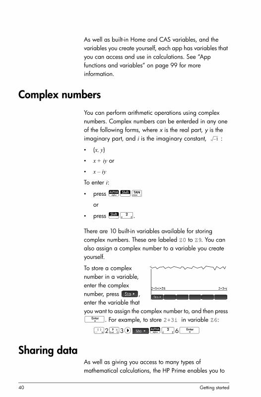
There are 10 built-in variables available for storing complex numbers. These are labeled Z0 to Z9. You can also assign a complex number to a variable you create yourself.
To store a complex number in a variable, enter the complex number, press , enter the variable that you want to assign the complex number to, and then press E. For example, to store 2+3i in variable Z6:
R2o3> Ay6E
Sharing dataAs well as giving you access to many types of mathematical calculations, the HP Prime enables you to
1–

Getting started 41
create various objects that can be saved and used over and over again. For example, you can create apps, lists, matrices, programs, and notes. You can also send these objects to other HP Primes. Whenever you encounter a screen with as a menu item, you can select an item on that screen to send it to another HP Prime.
You used the supplied USB cable to send objects from one HP Prime to another. Note that the connectors on the ends of the USB cable are slightly different. The micro-A connector has a rectangular end and the micro-B connector has a trapezoidal end. To share objects with another HP Prime, the micro-A connector must be inserted into the USB port on the sending calculator, with the micro-B connector inserted into the USB port on the receiving calculator.
General procedure The general procedure for sharing objects is as follows:
1. Navigate to the screen that lists the object you want to send.
This will be the Application Library for apps, the List Catalog for lists, the Matrix Catalog for matrices, the Program Catalog for programs, and the Notes Catalog for notes.
2. Connect the USB cable between the two calculators.
The micro-A connector—with the rectangular end—must be inserted into the USB port on the sending calculator.
3. On the sending calculator, highlight the object you want to send and tap .
In the illustration at the right, a program named TriangleCalcs has been selected in the Program Catalog
Micro-A: sender Micro-B: receiver

42 Getting started
and will be sent to the connected calculator when is tapped.
4. What happens on the receiving calc?
Online Help Press W to open the online help. The help initially provided is context-sensitive, that is, it is always about the current view and its menu items.
For example, to get help on the Function app, press I, select Function, and press W.
From within the help system you can navigate to other help topics. You can find help on any key, view, or command. And tapping displays a hierarchical directory of all the help topics.
Reverse Polish Notation (RPN) 43
2
Reverse Polish Notation (RPN)
The HP Prime provides you with three ways of entering objects in Home view:
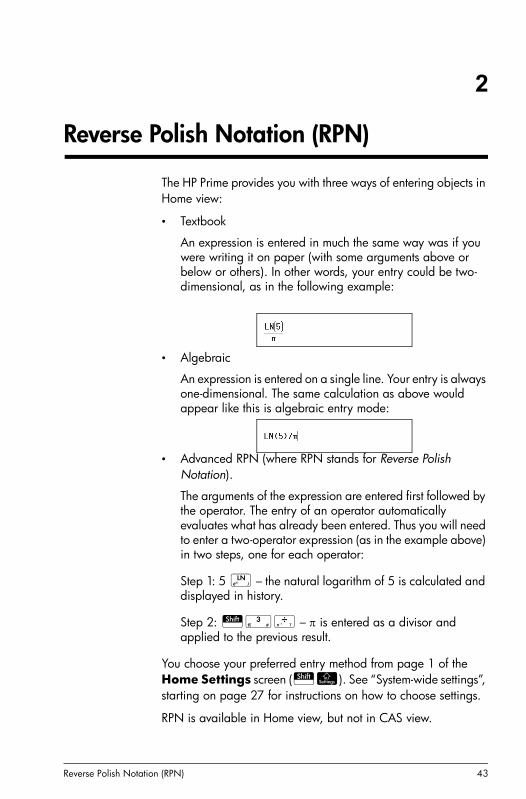
• Textbook
An expression is entered in much the same way was if you were writing it on paper (with some arguments above or below or others). In other words, your entry could be two-dimensional, as in the following example:
• Algebraic
An expression is entered on a single line. Your entry is always one-dimensional. The same calculation as above would appear like this is algebraic entry mode:
• Advanced RPN (where RPN stands for Reverse Polish Notation).
The arguments of the expression are entered first followed by the operator. The entry of an operator automatically evaluates what has already been entered. Thus you will need to enter a two-operator expression (as in the example above) in two steps, one for each operator:
Step 1: 5 h – the natural logarithm of 5 is calculated and displayed in history.
Step 2: Szn – is entered as a divisor and applied to the previous result.
You choose your preferred entry method from page 1 of the Home Settings screen (SH). See “System-wide settings”, starting on page 27 for instructions on how to choose settings.
RPN is available in Home view, but not in CAS view.

44 Reverse Polish Notation (RPN)
The same entry-line editing tools are available in RPN mode as in algebraic and textbook mode:
• Press C to delete the character to the left of the cursor.
• Press SC to delete the character to the right of the cursor.
• Press J to clear the entire entry line.
• Press SJ to clear the entire entry line.
History in RPN modeThe results of your calculations are kept in history. This history is displayed above the entry line (and by scrolling up to calculations that are no longer immediately visible). The calculator offers three histories: one for the CAS view and two for Home view. CAS history is discussed in chapter 3. The two histories in Home view are:
• non-RPN: visible if you have chosen algebraic or textbook as your preferred entry technique
• RPN: visible only if you have chosen RPN as your preferred entry technique. The RPN history is also called the stack. As shown in the illustration below, each entry in the stack is given a number. This is the stack level number.
As more calculations are added, an entry’s stack level number increases.
If you switch from RPN to algebraic or textbook entry, your history is not lost. It is just not visible. If you switch back to RPN, your RPN history is redisplayed. Likewise, if you switch to RPN, your non-RPN history is not lost.
When you are not in RPN mode, your history is ordered chronologically: oldest calculations at the top, most recent at the

Reverse Polish Notation (RPN) 45
bottom. In RPN mode, your history is ordered chronologically by default, but you can change the order of the items in history. (This is explained in “Manipulating the stack” on page 47.)
Re-using results
There ate two ways to re-use a result in history. Method 1 deselects the copied result after copying; method 2 keeps the copied item selected.
Method 1
1. Select the result to be copied. You can do this by pressing = or \ until the result is highlighted, or by tapping on it.
2. Press E. The result is copied to the entry line and is deselected.
Method 2
1. Select the result to be copied. You can do this by pressing = or \ until the result is highlighted, or by tapping on it.
2. Tap and select ECHO. The result is copied to the entry line and remains selected.
Although it might appear that only the result of the previous calculation is copied to the entry line, the calculation that produced that result is copied as well and becomes part of the new calculation. This is so regardless of the method chosen to copy the item.
Note that while you can copy an item from the CAS history to use in a Home calculation (and copy an item from the Home history to use in a CAS calculation), you cannot copy items from or to the RPN history. You can, however, use CAS commands and functions when working in RPN mode.
Re-using calculations
As well as re-using results (discussed in the previous section), you can copy an entire calculation. The copy is placed on stack level 1 and thus can easily be incorporated in your next calculation. You can also move an item to stack level 1. These changes to the stack are explained in “Manipulating the stack” on page 47.
Sample calculationsThe general philosophy behind RPN is that arguments are placed before operators. The arguments can be on the entry line

46 Reverse Polish Notation (RPN)
(each separated by a space) or they can be in history. For example, to multiply by 3, you could enter:
SzX 3
on the entry line and then enter the operator (s). Thus your entry line would look like this before entering the operator:
However, you could also have entered the arguments separately and then, with a blank entry line, entered the operator (s). Your history would look like this before entering the operator:
If there are no entries in history and you enter an operator or function, an error message appears. An error message will also appear if there is an entry on a stack level that an operator needs but it is not an appropriate argument for that operator. For example, pressing f when there is a string on level 1 displays an error message.
An operator or function will work only on the minimum number of arguments necessary to produce a result. Thus if you enter on the entry line 2 4 6 8 and press s, stack level 1 shows 48. Multiplication needs only two arguments, so the two arguments last entered are the ones that get multiplied. The entries 2 and 4 are not ignored: 2 is placed on stack level 3 and 4 on stack level 2.
Where a function can accept a variable number of arguments, you need to specify how many arguments you want it to include in its operation. You do this by specifying the number in parentheses straight after the function name. You then press E to evaluate the function. For example, suppose your stack looks like this:

Reverse Polish Notation (RPN) 47
Suppose further that you want to determine the minimum of just the numbers on stack levels 1, 2, and 3. You choose the MIN function from the MATH menu and complete the entry as MIN(3). When you press E, the minimum of just the last three items on the stack is displayed.
Manipulating the stackA number of stack-manipulation options are available. Most appear as menu items across the bottom the screen. To see these items, you must first select an item in history:
PICK Copies the selected item to stack level 1. The item below the one that is copied is then highlighted. Thus if you tapped four times, four consecutive items will be moved to the bottom four stack levels (levels 1–4).
ROLL There are two roll commads:
• Tap to move the selected item to stack level 1. This is similar to PICK, but PICK duplicates the item, with the duplicate being placed on stack level1. However, ROLL doesn’t duplicate an item. It simply moves it.
• Tap to move the item on stack level 1 to the currently highlighted level
48 Reverse Polish Notation (RPN)
Swap You can swap the position of the objects on stack level 1 with those on stack level 2. Just press o. The level of other objects remains unchanged. Note that the entry line must not be active at the time, otherwise a comma will be entered.
Stack Tapping displays further stack-manipulation tools.
DROPN Deletes all items in the stack from the highlighted item down to and including the item on stack level 1. Items above the highlighted item drop down to fill the levels of the deleted items.
If you just want to delete a single item from the stack, see “Delete an item” below.
DUPN Duplicates all items between (and including) the highlighted item and the item on stack level 1. If, for example, you have selected the item on stack level 3, selecting DUPN duplicates it and the two items below it, places them on stack levels 1 to 3, and moves the items that were duplicated up to stack levels 4 to 6.
Echo Places a copy of the selected result on the entry line and leaves the source result highlighted. [Not working]
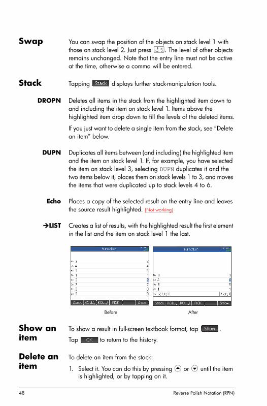
LIST Creates a list of results, with the highlighted result the first element in the list and the item on stack level 1 the last.
Show an item
To show a result in full-screen textbook format, tap .
Tap to return to the history.
Delete an item
To delete an item from the stack:
1. Select it. You can do this by pressing = or \ until the item is highlighted, or by tapping on it.
Before After

Reverse Polish Notation (RPN) 49
2. Press C.
Delete all items
To delete all items, thereby clearing the history, press SJ.

50 Reverse Polish Notation (RPN)

Computer algebra system (CAS) 51
3
Computer algebra system (CAS)
A computer algebra system (CAS) enables you to perform symbolic calculations. By default, CAS works in exact mode, giving you infinite precision. On the other hand, non-CAS calculations, such as those performed in HOME view or by an aplet, are numerical calculations and are often approximations limited by the precision of the calculator (to
in the case of the HP Prime). For example, yields the approximate answer .619047619047 in Home view (with Standard numerical format), but yields the exact answer in the CAS.
The CAS offers many hundreds of functions, covering algebra, calculus, equation solving, polynomials, and more. You select a function from the CAS menu, one of the Toolbox menus discussed in chapter 20, “Functions and commands”, beginning on page 283. Consult that chapter for a description of all the CAS functions and commands.
CAS viewCAS calculations are done in CAS view. CAS view is almost identical to Home view. A history of calculations is built and you can select and copy previous calculations just as you can in Home view, as well as store objects in variables.
To open CAS view, press K. CAS appears in red at the left of the title bar to indicate that you are in CAS view rather than Home view.
The menu buttons in CAS view are:
• : assigns an object to a variable
10 12– 13--- 2
7---+
1321------

52 Computer algebra system (CAS)
• : applies common simplification rules to reduce an expression to its simplest form. For example, simplify(ea + LN(b*ec)) yields b*EXP(a)*EXP(c).
• : copies a selected entry ion history to the entry line
• : displays the selected entry in full-screen mode, with horizontal land vertical scrolling enabled. The entry is also presented in textbook format.
CAS calculationsWith one exception, you perform calculations in CAS view just as you do in Home view. (The exception is that there is no RPN entry mode in CAS view, just algebraic and textbook modes). All the keys work in the same way in CAS view as Home view. The primary difference is that the default display of answers is symbolic rather than numeric.
You can also use the template key (F) to help you insert the framework for common calculations (and for vectors and matrices). This is explained in detail in “Math template” on page 21.
The most commonly used CAS functions are available from the CAS menu, one of the Toolbox menus. To display the menu, press D. (If the CAS menu is not open by default, tap
.) Other CAS commands are available from the CATLG menu (another of the Toolbox menus).
To choose a function, select a category and then a command.
Example 1 To find the roots of 2x2 + 3x – 2:
1. With the CAS menu open, select Polynomial and then Find Roots.
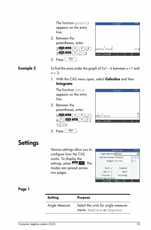
Computer algebra system (CAS) 53
The function proot() appears on the entry line.
2. Between the parentheses, enter:
2ASsj+3ASsw2
3. Press E.
Example 2 To find the area under the graph of 5x2 – 6 between x =1 and x = 3:
1. With the CAS menu open, select Calculus and then Integrate.
The function int() appears on the entry line.
2. Between the parentheses, enter:
5ASsjw6oASso1o3
3. Press E.
SettingsVarious settings allow you to configure how the CAS works. To display the settings, press SK. The modes are spread across two pages.
Page 1
Setting Purpose
Angle Measure Select the units for angle measure-ments: Radians or Degrees.

54 Computer algebra system (CAS)
Number Format (first drop-down list)
Select the number format for dis-played solutions: Standard or Scientific or Engineering
Number Format (second drop-down list)
Select the number of digits to dis-play in approximate mode (man-tissa + exponent).
Integers (drop-down list)
Select the integer base: Decimal (base 10)Hex (base 16)Octal (base 8)
Integers (check box)
If checked, any real number equiv-alent to an integer in a non-CAS environment will be converted to an integer in the CAS. (Real num-bers not equivalent to integers are treated as real numbers in CAS whether or not this option is selected.)
Exact If checked, the calculator is in exact mode and solutions will be symbolic. If not checked, the calcu-lator is in approximate mode and solutions will be approximate. For example, 26n5 yields in exact mode and 5.2 in approxi-mate mode.
Complex Select this to allow complex results in variables.
Use √ If checked, second order polyno-mials are factorized in complex mode or in real mode if the dis-criminant is positive.
Setting Purpose (Cont.)
265
-----------
Computer algebra system (CAS) 55
Page 2
Use i If checked, the calculator is in complex mode and complex solu-tions will be displayed when they exist. If not checked, the calculator is in real mode and only real solu-tions will be displayed. For exam-ple, factors(x4–1) yields(–1+x),(1+x),(i+x),(–i+x) in com-plex mode and (–1+x),(1+x),(1+x2) in real mode.
Principal If checked, the principal solutions to trigonometric functions will be displayed. If not checked, the gen-eral solutions to trigonometric func-tions will be displayed.
Increasing If checked, polynomials will be displayed with increasing powers (for example, –4+x+3x2+x3). If not checked, polynomials will be dis-played with decreasing powers (for example, x3+3x2+x–4).
Setting Purpose (Cont.)
Setting Purpose
Recursive Evaluation
Specify the maximum number of embedded variables allowed in an interactive evaluation. See also Recursive Replacement below.
Recursive Replacement
Specify the maximum number of embedded variables allowed in a single evaluation in a program. See also Recursive Evalua-tion above.
Recursive Function
Specify the maximum number of embedded function calls allowed.

56 Computer algebra system (CAS)
Setting the form of menu items
One setting that affects the CAS is made outside the CAS Settings screen. This setting determines whether the commands on the CAS menu are presented descriptively or by their command name. Here are some examples of identical functions that are presently differently depending on what presentation mode you select:
The default menu presentation mode is to provide the descriptive names for the CAS functions. If you prefer the functions to be presented by their command name, deselect the Menu Display option on the second page of the Home Settings screen (see “Home settings” on page 27).
To use an expression or result from Home view
When your are working in CAS, you can retrieve an expres-sion or result from Home view by tapping Z and selectingGet from Home. Home view opens. Press = or \ untilthe item you want to retrieve is highlighted and press E.
Epsilon Any number smaller than the value specified for epsilon will be shown as zero.
Probability Specify the maximum probability of an answer being wrong for non-deterministic algorithms. Set this to zero for deterministic algo-rithms.
Newton Specify the maximum number of iterations when using the Newto-nian method to find the roots of a quadratic.
Setting Purpose (Cont.)
Descriptive name Command name
Factors List ifactors
Complex Zeros cZeros
Groebner Basis gbasis
Factor by Degree factor_xn
Find Roots proot

Computer algebra system (CAS) 57
The highlighted item is copied to the cursor point in CAS.
To use a Home variable in CAS
You can access Home variables from within the CAS. Home variables are assigned uppercase letters; CAS variables are assigned lowercase letters. Thus SIN(x) and SIN(X) will yield different results.
To use a Home variable in the CAS, simply include its name in a calculation. For example, suppose in Home view you have assigned variable Q to 100. Suppose too that you have assigned variable q to 1000 in the CAS. If you are in the CAS and enter 5*q, the result is 5000. If had entered 5*Q instead, the result would be 500.
In a similar way, CAS variables can be used in calculations in Home view. Thus you can enter 5*q in Home view and get 500, even though q is a CAS variable.

58 Computer algebra system (CAS)
An introduction to HP apps 59
4
An introduction to HP apps
Much of the functionality of the HP Prime is provided in packages called HP apps. The HP Prime comes with 18 HP apps: 10 dedicated to mathematical topics or tasks, three specialized Solvers, three function Explorers, a spreadsheet, and an app for recording data streamed to the calculator from an external sensing device. You launch an app by first pressing I (which displays the Application Library screen) and tapping on the icon for the app you want.
What each app enables you to do is outlined in the following, where the apps are listed in alphabetical order.
App name Use this app to:
Advanced Graphing
Explore the graphs of symbolic open sentences in x and y. Example:
Data Streamer Collect real-world data from scientific sensors and export it to a statistics app for analysis.
Finance Solve time-value-of-money (TVM) problems and amortization problems.
Function Explore real-valued, rectangular functions of y in terms of x. Example:
Geometry Explore geometric constructions and perform geometric calculations.
Inference Explore confidence intervals and hypothesis tests based on the Normal and Student’s-t distributions.
Linear Explorer Explore the properties of linear equations and test your knowledge.
x2 y2+ 64=
y 2x2 3x 5+ +=

60 An introduction to HP apps
As you use an app to explore a lesson or solve a problem, you add data and definitions in one or more of the app’s views. All this information is automatically saved in the app. You can come back to the app at any time and all the information is still there. You can also save a version of the app with a name you give it and then use the original app for another problem or purpose. See “Creating an app” on page 97 for more information about customizing and saving apps.
Linear Solver Find solutions to sets of two or three linear equations.
Parametric Explore parametric functions of x and y in terms of t. Example: x = cos (t) and y = sin(t).
Polar Explore polar functions of r in terms of an angle . Example:
Quadratics Explorer
Explore the properties of quadratic equations and test your knowledge.
Sequence Explore sequence functions, where U is defined in terms of n, or in terms of previous terms in the same or another sequence, such as and . Example: , and
Solve Explore equations in one or more real-valued variables, and systems of equations. Example:
Spreadsheet To solve problems or represent data best suited to a spreadsheet.
Statistics 1Var Calculate one-variable statistical data (x)
Statistics 2Var Calculate two-variable statistical data (x and y)
Triangle Solver Find the unknown values for the lengths and angles of triangles.
Trig Explorer Explore the properties of sinusoidal equations and test your knowledge.
App name Use this app to: (Cont.)
r 2 4 cos=
Un 1– Un 2–
U1 0= U2 1=Un Un 2– Un 1–+=
x 1+ x2 x– 2–=

An introduction to HP apps 61
With one exception, all the apps mentioned above are described in detail in this user guide. The exception is the DataStreamer app. A brief introduction to this app is given in the HP Prime Quick Start Guide. Full details can be found in the HP StreamSmart 410 User Guide (available on the product CD).
Application LibraryApps are stored in the Application Library, displayed by pressing I.
To open an app
1. Open the Application Library.
2. Find the app’s icon and tap on it.
You can also use the cursor keys to scroll to the app and, when it is highlighted, either tap or press E.
To reset an app
You can leave an app at any time and all the data and settings in it are retained. When you return to the app, you can continue as you left off.
However, if you don’t want to use the previous data and settings, you can return the app to its default state, that is, the state it was in when you opened it for the first time. To do this:
1. Open the Application Library.
2. Use the cursor keys to highlight the app.
3. Tap .
4. Tap to confirm your intention.
You can also reset an app from within the app. From the main view of the app—which is usually, but not always, the Symbolic view—press SJ and tap to confirm your intention.
To sort apps By default, the apps in the Application Library are sorted chronologically, with the most recently used app shown first. You can change the sort order to:
• Alphabetically
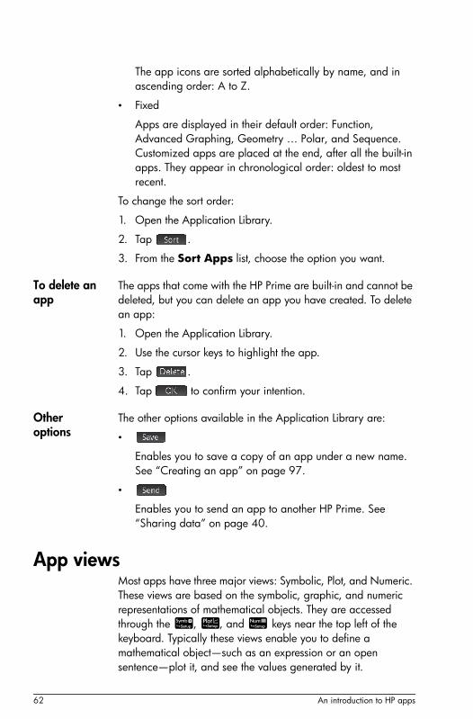
62 An introduction to HP apps
The app icons are sorted alphabetically by name, and in ascending order: A to Z.
• Fixed
Apps are displayed in their default order: Function, Advanced Graphing, Geometry … Polar, and Sequence. Customized apps are placed at the end, after all the built-in apps. They appear in chronological order: oldest to most recent.
To change the sort order:
1. Open the Application Library.
2. Tap .
3. From the Sort Apps list, choose the option you want.
To delete an app
The apps that come with the HP Prime are built-in and cannot be deleted, but you can delete an app you have created. To delete an app:
1. Open the Application Library.
2. Use the cursor keys to highlight the app.
3. Tap .
4. Tap to confirm your intention.
Other options
The other options available in the Application Library are:
•
Enables you to save a copy of an app under a new name. See “Creating an app” on page 97.
•
Enables you to send an app to another HP Prime. See “Sharing data” on page 40.
App viewsMost apps have three major views: Symbolic, Plot, and Numeric. These views are based on the symbolic, graphic, and numeric representations of mathematical objects. They are accessed through the Y, P, and M keys near the top left of the keyboard. Typically these views enable you to define a mathematical object—such as an expression or an open sentence—plot it, and see the values generated by it.

An introduction to HP apps 63
Each of these views has an accompanying setup view, a view that enables you to configure the appearance of the data in the accompanying major view. These views are called Symbolic Setup, Plot Setup, and Numeric Setup. They are accessed by pressing JY, JP, and JM.
Not all apps have all the six views outlined above. The scope and complexity of each app determines its particular set of views. For example, the Spreadsheet app has no Plot view or Plot Setup view, and the Quadratic Explorer has only a Plot view. What views are available in each app is outlined in the next six sections.
Note that the DataStreamer app is not covered in this chapter. See HP StreamSmart 410 User Guide for information about this app.
Symbolic viewThe table below outlines what is done in the Symbolic view of each app.
App Use the Symbolic view to:
Advanced Graphing
Specify up to 10 open sentences.
Finance Not used
Function Specify up to 10 real-valued, rectangular functions of y in terms of x.
Geometry View the symbolic definition of geometric constructions.
Inference Choose to conduct a hypothesis test or test a confidence level, and select a type of test.
Linear Explorer Not used
Linear Solver Not used
Parametric Specify up to 10 parametric functions of x and y in terms of t.
Polar Specify up to 10 polar functions of r in terms of an angle .

64 An introduction to HP apps
Symbolic Setup viewThe Symbolic Setup view is the same for each app. It enables you to override the system-wide settings for angle measure, number format, and complex-number entry. The override applies only to the current app.
To change the settings for all apps, see “System-wide settings” on page 27.
Plot viewThe table below outlines what is done in the Plot view of each app.
Quadratics Explorer
Not used
Sequence Specify up to 10 sequence functions.
Solve Specify up to 10 equations.
Spreadsheet Not used
Statistics 1Var Specify up to 5 univariate analyses.
Statistics 2Var Specify up to 5 multivariate analyses.
Triangle Solver Not used
Trig Explorer Not used
App Use the Symbolic view to: (Cont.)
App Use the Polar view to:
Advanced Graphing
Plot and explore the open sentences selected in Symbolic view.
Finance Display an amortization graph.
Function Plot and explore the functions selected in Symbolic view.
Geometry Create and manipulate geometric constructions.
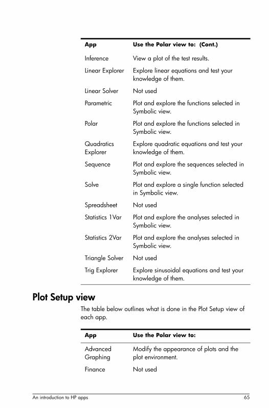
An introduction to HP apps 65
Plot Setup viewThe table below outlines what is done in the Plot Setup view of each app.
Inference View a plot of the test results.
Linear Explorer Explore linear equations and test your knowledge of them.
Linear Solver Not used
Parametric Plot and explore the functions selected in Symbolic view.
Polar Plot and explore the functions selected in Symbolic view.
Quadratics Explorer
Explore quadratic equations and test your knowledge of them.
Sequence Plot and explore the sequences selected in Symbolic view.
Solve Plot and explore a single function selected in Symbolic view.
Spreadsheet Not used
Statistics 1Var Plot and explore the analyses selected in Symbolic view.
Statistics 2Var Plot and explore the analyses selected in Symbolic view.
Triangle Solver Not used
Trig Explorer Explore sinusoidal equations and test your knowledge of them.
App Use the Polar view to: (Cont.)
App Use the Polar view to:
Advanced Graphing
Modify the appearance of plots and the plot environment.
Finance Not used
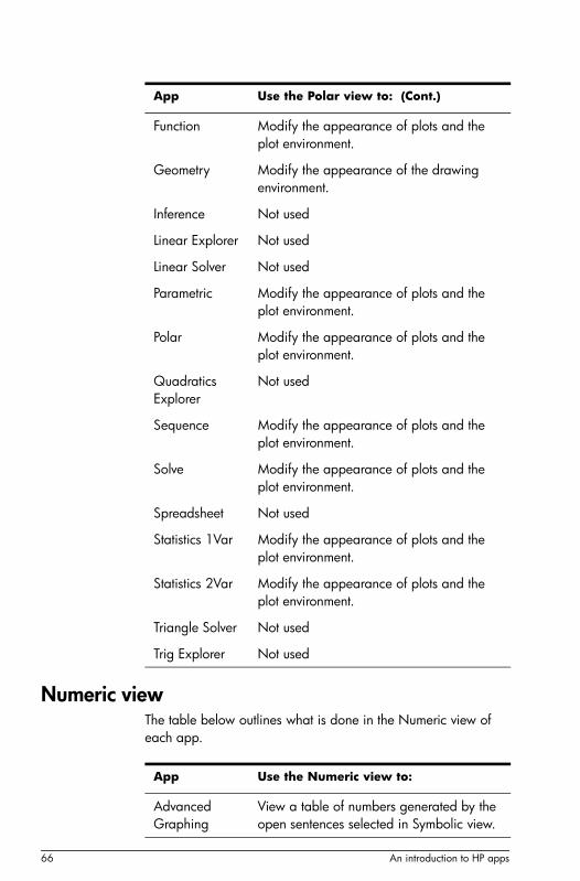
66 An introduction to HP apps
Numeric viewThe table below outlines what is done in the Numeric view of each app.
Function Modify the appearance of plots and the plot environment.
Geometry Modify the appearance of the drawing environment.
Inference Not used
Linear Explorer Not used
Linear Solver Not used
Parametric Modify the appearance of plots and the plot environment.
Polar Modify the appearance of plots and the plot environment.
Quadratics Explorer
Not used
Sequence Modify the appearance of plots and the plot environment.
Solve Modify the appearance of plots and the plot environment.
Spreadsheet Not used
Statistics 1Var Modify the appearance of plots and the plot environment.
Statistics 2Var Modify the appearance of plots and the plot environment.
Triangle Solver Not used
Trig Explorer Not used
App Use the Polar view to: (Cont.)
App Use the Numeric view to:
Advanced Graphing
View a table of numbers generated by the open sentences selected in Symbolic view.

An introduction to HP apps 67
Finance Enter values for time-value-of-money calculations.
Function View a table of numbers generated by the functions selected in Symbolic view.
Geometry Perform calculations on the geometric objects drawn in Plot view.
Inference Specify the statistics needed to perform the test selected in Symbolic view.
Linear Explorer Not used
Linear Solver Specify the coefficients of the linear equations to be solved.
Parametric View a table of numbers generated by the functions selected in Symbolic view.
Polar View a table of numbers generated by the functions selected in Symbolic view.
Quadratics Explorer
Not used
Sequence View a table of numbers generated by the sequences selected in Symbolic view.
Solve Enter the known values and solve for the unknown value.
Spreadsheet Enter numbers, text, formulas, etc. The Numeric view is the primary view for this app.
Statistics 1Var Enter data for analysis.
Statistics 2Var Enter data for analysis.
Triangle Solver Enter known data about a triangle and solve for the unknown data.
Trig Explorer Not used
App Use the Numeric view to: (Cont.)

68 An introduction to HP apps
Numeric Setup viewThe table below outlines what is done in the Numeric Setup view of each app.
App Use the Numeric Setup view to:
Advanced Graphing
Specify the numbers to be calculated according to the open sentences specified in Symbolic view, and set the zoom factor.
Finance Not used.
Function Specify the numbers to be calculated according to the functions specified in Symbolic view, and set the zoom factor.
Geometry Not used
Inference Not used
Linear Explorer Not used
Linear Solver Not used
Parametric Specify the numbers to be calculated according to the functions specified in Symbolic view, and set the zoom factor.
Polar Specify the numbers to be calculated according to the functions specified in Symbolic view, and set the zoom factor.
Quadratics Explorer
Not used.
Sequence Specify the numbers to be calculated according to the sequences specified in Symbolic view, and set the zoom factor.
Solve Not used
Spreadsheet Format cells, rows, columns, or the entire spreadsheet.
Statistics 1Var Not used
Statistics 2Var Not used
Triangle Solver Not used

An introduction to HP apps 69
Quick exampleThe following example uses all six app views and should give you an idea of the typical workflow involved in working with an app. The Polar app is used as the sample app.
Open the app
1. Open the Application Library by pressing I.
2. Tap once on the icon of the Polar app.
The Polar app opens in Symbolic View.
Symbolic view
The Symbolic view of the Polar app is where you define or specify the polar equation you want to plot and explore. In this example we will plot and explore the equation
3. Define the equation by entering:
4Szfn2>>f>jE
This equation will draw symmetrical petals provided that the angle measure is set to radians. The angle measure for this app is set in the Symbolic Setup view.
Symbolic Setup view
4. Press SY.
5. Select Radians from the Angle Measure menu.
Trig Explorer Not used
App Use the Numeric Setup view to: (Cont.)
r 4 2 2coscos=
r 4 2 2coscos=

70 An introduction to HP apps
Plot view
6. Press P.
A graph of the equation is plotted. However, as the illustration at the right shows, only a part of the petals is visible. To see the rest you will need to change the plot setup parameters.
Plot Setup View
7. Press SP.
8. Set the second RNG field to 4 by entering:
>4Sz (
9. Press P to return to Plot view and see the complete plot.
Numeric View
The values generated by the equation can be seen in Numeric view.
10. Press M.
Suppose you want to see just whole numbers for ; in other words, you want the increment between consecutive values in the column to be 1. You set this up in the Numeric Setup view.

An introduction to HP apps 71
Numeric Setup View
11. Press SM.
12. Change the NUMSTEP field to 1.
13. Press M to return to Numeric view.
You will see that the column now contains consecutive integers starting from zero, and the corresponding values calculated by the equation specified in Symbolic view are listed in the R1 column.
Common operations in Symbolic view [Scope: Advanced Graphing, Function, Parametric, Polar, Sequence, Solve. See dedicated app chapters for information about the other apps.]
Symbolic view functionality that is common to many apps is described in detail in this section. Functionality that is available only in a particular app is described in the chapter dedicated to that app.
Symbolic view is typically used to define a function or open sentence that you want to explore (by plotting and/or evaluating). In this section, the term definition will be used to cover both functions and open sentences.
Press Y to open Symbolic view.
Add a definition
With the exception of the Parametric app, there are 10 fields for entering definitions. In the Parametric app there are 20 fields, two for each paired definition.
1. Highlight an empty field you want to use, either by tapping on it or scrolling to it.
2. Enter your definition.
If you need help, see “Definitional building blocks” on page 72.
3. Tap or press E when you have finished.

72 An introduction to HP apps
Your new definition is added to the list of definitions.
Note that variables used in definitions must be in uppercase. A variable entered in lowercase will cause an error message to appear.
Modify a definition
1. Highlight the definition you want to modify, either by tapping on it or scrolling to it.
2. Tap .
The definition is copied to the entry line.
3. Modify the definition.
4. Tap or press E when you have finished.
Definitional building blocks
The components that make up a symbolic definition can come from a number of sources.
• From the keyboard
You can enter components directly from the keyboard. To enter 2X2 – 3, just press 2AXjw3.
• From user variables
If, for example, you have created a variable called COST, you could incorporate that into a definition either by typing it or choosing it from the User menu (one of the sub-menus of the Variables menu). Thus you could have a definition that reads F1(X)=X2+COST.
To select a user variable, press a, tap , select User Variables, and then select the variable of interest.
• From Home variables
Some Home variables can be incorporated into a symbolic definition. To access a Home variable, press a, tap
, select a category of variable, and select the variable of interest. Thus you could have a definition that reads F1(X)=X2+Q. (Q is on the Real sub-menu of the Home menu.)
Home variables are discussed in detail in chapter 28, “Troubleshooting”, beginning on page 507.
• From app variables

An introduction to HP apps 73
All settings, definitions, and results, for all apps, are stored as variables. Many of these variables can be incorporated into a symbolic definition. To access app variables, press a, tap , select the app, select the category of variable, and then select the variable of interest. You could, for instance, have a definition that reads F2(X)=X2+X–Root. The value of the last root calculated in the Function app is substituted for Root when this definition is evaluated.
App variables are discussed in detail in chapter 28, “Troubleshooting”, beginning on page 507.
• From math functions
Some of the functions on the Math menu can be incorporated into a definition. The Math menu is one of the Toolbox menus (D). The following definition combines a math function (Size) with a Home variable (L1): F4(X)=X2–SIZE(L1). It is equivalent to x2 – n where n is the number of elements in the list named L1. (Size is an option on the List menu, which is a sub-menu of the Math menu.)
• From CAS functions
Some of the functions on the CAS menu can be incorporated into a definition. The CAS menu is one of the Toolbox menus (D). The following definition incorporates the CAS function irem: F5(X)=X2+CAS.irem(45,7). (irem is entered by choosing Remainder, an option on the Division menu, which is a sub-menu of the Integer menu. Note that any CAS command or function selected to operate outside the CAS is given the CAS. prefix.)
• From app functions
Some of the functions on the App menu can be incorporated into a definition. The App menu is one of the Toolbox menus (D). The following definition incorporates the app function PredY:
F9(X)=X2+Statistics_2Var.PredY(6).
• From the Catlg menu
Some of the functions on the Catlg menu can be incorporated into a definition. The Catlg menu is one of the Toolbox menus (D). The following definition incorporates

74 An introduction to HP apps
a command from that menu and an app variable: F6(X)=X2+INT(Root). The integer value of the last root calculated in the Function app is substituted for INT(Root) when this definition is evaluated.
• From other definitions
You could, for example, define F3(X)as F1(X)*F2(X).
Evaluate a dependent definition
If you have a dependent definition—that is, one defined in terms of another definition—you can combine all the definitions into one by evaluating the dependent definition.
1. Select the dependent expression.
2. Tap .
Consider the example at the right. Notice that F3(X)is defined in terms of two other functions. It is a dependent definition and can be evaluated. If you highlight F3(X)and tap
, F3(X)becomes 2*X2+X+ 2*(X2–1).
Select or deselect a definition to explore
In the Advanced Graphing, Function, Parametric, Polar, Sequence, and Solve apps you can enter up to 10 definitions. However, only those definitions that are selected in Symbolic view will be plotted in Plot view and evaluated in Numeric view.
You can tell if a definition is selected by the tick (or checkmark) beside it. A checkmark is added by default as soon as you create a definition. So if you don’t want to plot or evaluate a particular definition, highlight it and tap . (Do likewise if you want to re-select a deselected function.)
Choose a color for plots
Each function and open sentence can be plotted in a different color. If you want to change the default color of a plot:

An introduction to HP apps 75
1. Tap the colored square to the left of the function’s definition.
You can also select the square by pressing E while the definition is selected. Pressing E moves the selection from the definition to the colored square and from the colored square to the definition.
2. tap .
3. Select the desired color from the color-picker.
Delete a definition
To delete a single definition:
1. Tap once on it (or highlight it using the cursor keys).
2. Press C.
To delete all the definitions:
1. Press SJ.
2. Tap or press E to confirm your intention.

76 An introduction to HP apps
Symbolic view: Summary of menu buttons
Common operations in Symbolic Setup view
Button Purpose
Copies the highlighted definition to the entry line for editing. Tap when done. To add a new definition—even one that is replacing an existing one—highlight the field and just start entering your new definition.
Selects (or deselects) a definition.
[Function only]
Enters the independent variable in the Function app. You can also press d.
[Advanced Graphing only]
Enters an X in the Advanced Graphing app. You can also press d.
[Advanced Graphing only]
Enters an Y in the Advanced Graphing app.
[Parametric only]
Enters the independent variable in the Parametric app. You can also press d.
[Polar only]
Enters the independent variable in the Polar app. You can also press d.
[Sequence only]
Enters the independent variable in the Sequence app. You can also press d.
[Solve only]Enters the equals sign in the Solve app. A shortcut equivalent to pressing S..
Displays the selected definition in full-screen mode. See “Large results” on page 36 for more information.
Evaluates dependent definitions. See “Evaluate a dependent definition” on page 74.

An introduction to HP apps 77
[Scope: all apps]
The Symbolic Setup view is the same for all apps. Its primary purpose is to allow you to override three of the system-wide settings specified on the Home Settings window.
Press SY to open Symbolic Setup view.
Override system-wide settings
1. Tap once on the setting you want to change.
You can tap on the field name or the field.
2. Tap again on the setting.
A menu of options appears.
3. Select the new setting.
Note that selecting the Fixed, Scientific, or Engineering option on the Number Format menu displays a second field for you to enter the required number of significant digits.
You could also select a field, tap , and select the new setting.
Restore default settings
To restore default settings is to return precedence to the settings on the Home Settings screen.
To restore one field to its default setting:
1. Select the field.
2. Press C.
To restore all default settings, press SJ.
Common operations in Plot view Plot view functionality that is common to many apps is described in detail in this section. Functionality that is available only in a particular app is described in the chapter dedicated to that app.
Press P to open Plot view.

78 An introduction to HP apps
Zoom [Scope: Advanced Graphing, Function, Parametric, Polar, Sequence, Solve, Statistics 1 Var, and Statistics 2Var. Also, to a limited degree, Geometry.]
Zooming redraws the plot on a larger or smaller scale. It is a shortcut for changing the range settings in Plot Setup view. The extent of most zooms is determined by two zoom factors: a horizontal and a vertical factor. By default, these factors are both 2. Zooming out multiplies the scale by the factor, so that a greater scale distance appears on the screen. Zooming in divides the scale by the factor, so that a shorter scale distance appears on the screen.
Zoom factors To change the default zoom factors:
1. Open the Plot view of the app (P).
2. Tap to open the Plot view menu.
3. Tap to open the Zoom menu.
4. Scroll and select Set Factors.
The Zoom Factors screen appears.
5. Change one or both zoom factors.
6. If you want the plot to be centered around the current position of the cursor in Plot view, select Recenter.
7. Tap or press E.
Zoom options
Zoom options are available from three sources:
• the keyboard
• the menu in Plot view
• the Views menu (V).
Zoom keys There are two zoom keys: pressing + zooms in and pressing w zooms out. The extent of the scaling is determined by the ZOOM FACTOR settings (explained above).
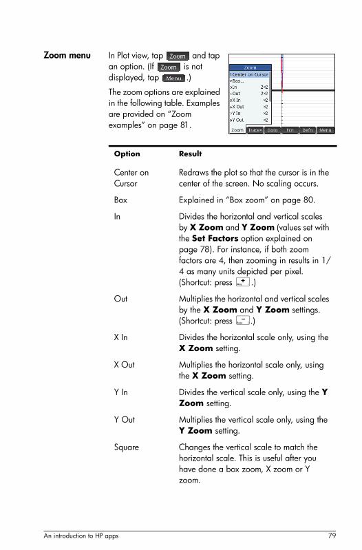
An introduction to HP apps 79
Zoom menu In Plot view, tap and tap an option. (If is not displayed, tap .)
The zoom options are explained in the following table. Examples are provided on “Zoom examples” on page 81.
Option Result
Center on Cursor
Redraws the plot so that the cursor is in the center of the screen. No scaling occurs.
Box Explained in “Box zoom” on page 80.
In Divides the horizontal and vertical scales by X Zoom and Y Zoom (values set with the Set Factors option explained on page 78). For instance, if both zoom factors are 4, then zooming in results in 1/4 as many units depicted per pixel. (Shortcut: press +.)
Out Multiplies the horizontal and vertical scales by the X Zoom and Y Zoom settings. (Shortcut: press w.)
X In Divides the horizontal scale only, using the X Zoom setting.
X Out Multiplies the horizontal scale only, using the X Zoom setting.
Y In Divides the vertical scale only, using the Y Zoom setting.
Y Out Multiplies the vertical scale only, using the Y Zoom setting.
Square Changes the vertical scale to match the horizontal scale. This is useful after you have done a box zoom, X zoom or Y zoom.

80 An introduction to HP apps
Box zoom A box zoom enables you to zoom in on an area of the screen that you specify.
1. With the Plot view menu open, tap and select Box.
2. Tap one corner of the area you want to zoom in on and then tap .
3. Tap the diagonally opposite corner of the area you want to zoom in on and then tap .
The screen fills with the area you specified. To return to the default view, tap and select Decimal.
Views menu The most commonly used zoom options are also available on the Views menu. These are:
• Autoscale
• Decimal
• Integer
• Trig.
Autoscale Rescales the vertical axis so that the display shows a representative piece of the plot given the supplied x axis settings. (For Sequence and Statistics apps, autoscaling rescales both axes.)The autoscale process uses the first selected function to determine the best scale to use.
Decimal Rescales both axes so each pixel is 0.1 units. This is equivalent to resetting the default values for XRNG and YRNG.
Integer Rescales the horizontal axis only, making each pixel equal to 1 unit.
Trig Rescales the horizontal axis so that 1 pixel equals /24 radians or 7.5 degrees; rescales the vertical axis so that 1 pixel equals 0.1 units.
Undo Zoom Returns the display to the previous zoom, or if there has been only one zoom, displays the graph with the original plot settings.
Option Result (Cont.)

An introduction to HP apps 81
These options—which can be applied whatever view you are currently working in—are explained in the table immediately above.
Testing a zoom with split-screen viewing
A useful way of testing a zoom is to divide the screen into two halves, with each half showing the plot, and then to apply a zoom only to one side of the screen. The illustration at the right is a plot of y = 3sin x. To split the screen into two halves:
1. Open the Views menu.
Press V
2. Select Split Screen: Plot Detail.
The result is shown at the right. Any zoom operation you undertake will be applied only to the copy of the plot in the right-hand half of the screen. This will help you test and then choose an appropriate zoom.
Note that you can replace the original plot on the left with the zoomed plot on the right by tapping .To un-split the screen, press P.
Zoom examples
The following examples show the effects of the zooming options on a plot of using the default zoom factors (2 × 2). Split-screen mode (described above) has been used to help you see the effect of zooming.
Note that there is an Unzoom option on the Zoom menu. Use this to return a plot to its pre-zoom state. If the Zoom menu is not shown, tap .
Zoom In
In
Shortcut: press +
3 xsin

82 An introduction to HP apps
Zoom Out
Out
Shortcut: press w
X In
XIn
X Out
X Out
Y In Y In
Y Out
Y Out

An introduction to HP apps 83
Square
Square
Notice that in this example, the plot on left has had a Y In zoom applied to it. The Square zoom has returned the plot to its default state where the X and Y scales are equal.
Autoscale
Autoscale
Decimal
Decimal
Notice that in this example, the plot on left has had a X In zoom applied to it. The Decimal zoom has reset the default values for the x-range and y-range.
Integer
Integer
Trig
Trig

84 An introduction to HP apps
Trace[Scope: Advanced Graphing, Function, Parametric, Polar, Sequence, Solve, Statistics 1 Var, and Statistics 2Var.]
The tracing functionality enables you to move a cursor (the trace cursor) along the current graph. You move the trace cursor by pressing < or >. You can also move the trace cursor by tapping on or near the current plot. The trace cursor jumps to the point on the plot that is closest point to where you tapped.
The current coordinates of the cursor are shown at the bottom of the screen. (If menu buttons are hiding the coordinates, tap
to hide the buttons.)
Trace mode and coordinate display are automatically turned on when a plot is drawn.
To select a plot
If there is more than one plot displayed, press = or \ until the trace cursor is on the plot you are interested in.
To evaluate a definition
One of the primary uses of the trace functionality is to evaluate a plotted definition. Suppose in Symbolic view you have defined F1(X) as (X–1)2–3. Suppose further that you want to know what the value of that function is when X is 25.
1. Open Plot view (P).
2. If the menu at the bottom of the screen is not open, tap .
3. If more than one definition is plotted, ensure that the trace cursor is on the plot of the definition you want to evaluate. You can press to see the definition of a plot, and press = or \ to move the trace cursor from plot to plot.
4. If you pressed to see the definition of a plot, the menu at the bottom of the screen will be closed. Tap to re-open it.
5. Tap .
6. Enter 25 and tap .
7. Tap .

An introduction to HP apps 85
The value of F1(X) when X is 25 us shown at the bottom of the screen. .
This is one of many ways the HP Prime provides for you to evaluate a function for a specific independent variable. You can also evaluate a function in Numeric view (see page 92). Moreover, any expression you define in Symbolic view can be evaluated in Home view. For example, suppose F1(X)is defined as (x – 1)2 – 3. If you enter F1(4) in Home view and press E you get 6, since (4– 1)2 – 3 = 6.
To turn tracing on or off
• To turn off tracing, tap .
• To turn on tracing, tap .
If these options are not displayed, tap .
When tracing is off, pressing the cursor keys no longer constrains the cursor to a plot.

86 An introduction to HP apps
Plot view: Summary of menu buttons
Common operations in Plot Setup view This section covers only operations common to the apps mentioned. See the chapter dedicated to an app for the app-specific operations done in Plot Setup view.
Press SP to open Plot Setup view.
Configure Plot view[Scope: Advanced Graphing, Function, Parametric, Polar, Sequence, Statistics 1 Var, Statistics 2Var]
The Plot Setup view is used to configure the appearance of Plot view and to set the method by which graphs are plotted. The
Button Purpose
Displays a menu of zoom options. See “Zoom options” on page 78.
A toggle button for turning off and turning on trace functionality. See “Trace” on page 84.
Displays an input form for you to specify a value you want the cursor to jump to. The value you enter is the value of the independent variable.
[Function only]
Displays a menu of options for analyzing a plot. See “Analyzing functions” on page 109.
Displays the definition responsible for generating the selected plot.
A toggle button that shows and hides the other buttons across the bottom of the screen.

An introduction to HP apps 87
configuration options are spread across two pages. Tap to move from the first to the second page, and to return to the first page.
T i p When you go to Plot view to see the graph of a definition selected in Symbolic view, there may be no graph shown. The likely cause of this is that the spread of plotted values is outside the range settings in Plot Setup view. A quick way to bring the graph into view is to press V and select Autoscale. This also changes the range settings in Plot Setup view.
Page 1 Setup field Purpose
TRNG
[Parametric only]
Sets the range of T-values to be plotted. Note that here are two fields: one for the minimum and one for the maximum value.
TSTEP [Parametric only]
Sets the increment between consecutive T-values.
RNG
[Polar only]Sets the range of angle values to be plotted. Note that here are two fields: one for the minimum and one for the maximum value.
STEP [Polar only]
Sets the increment between consecutive angle values.
SEQPLOT [Sequence only]
Sets the type of plot: Stairstep or Cobweb.
NRNG
[Sequence only]
Sets the range of N-values to be plotted. Note that here are two fields: one for the minimum and one for the maximum value.
HWIDTH
[Stats 1 Var only]
Sets the width of the bars in a histogram.
HRNG
[Stats 1 Var only]
Sets the range of values to be included in a histogram. Note that here are two fields: one for the minimum and one for the maximum value.

88 An introduction to HP apps
Page 2
S*MARK
[Stats 2 Var only]
Sets the graphic that will be used to represent a data point in a scatter plot. A different graphic can be used for each of the five analyses that can be plotted together.
XRNG Sets the initial range of the x-axis. Note that here are two fields: one for the minimum and one for the maximum value. In Plot view the range can be changed by panning and zooming.
YRNG Sets the initial range of the y-axis. Note that there are two fields: one for the minimum and one for the maximum value. In Plot view the range can be changed by panning and zooming.
XTICK Sets the increment between tickmarks on the x-axis.
YTICK Sets the increment between tickmarks on the y-axis.
Setup field Purpose (Cont.)
Setup field Purpose
AXES Shows or hides the axes.
LABELS Places values at the ends of each axis to show the current range of values.
GRID DOTS Places a dot at the intersection of each horizontal and vertical grid line.
GRID LINES Draws a horizontal and vertical grid line at each integer x-value and y-value.
CURSOR Sets the appearance of the trace cursor: standard, inverting, or blinking.
CONNECT
[Stats 2 Var only]
Connects the data points with straight segments.

An introduction to HP apps 89
Graphing methodsThe HP Prime gives you the option of choosing one of three graphing methods. The methods are described below, with each applied to the function f(x) = 9*sin(ex).
• adaptive: this gives very accurate results and is used by default. With this method active, some complex functions may take a while to plot. In these cases,
appears on the menu bar, enabling you to stop the plotting process if you wish.
• fixed-step segments: this method samples x-values, computes their corresponding y-values, and then plots and connects the points.
• fixed-step dots: this works like fixed-step segments method but does not connect the points.
Restore default settings[Scope: Advanced Graphing, Function, Parametric, Polar, Sequence, Solve, Statistics 1 Var, Statistics 2Var, Geometry.]
To restore one field to its default setting:
1. Select the field.
METHOD
[Not in either statistics app]
Sets the graphing method to adaptive, fixed-step segments, or fixed-step dots. Explained below.
Setup field Purpose (Cont.)

90 An introduction to HP apps
2. Press C.
To restore all default settings, press SJ.
Common operations in Numeric view [Scope: Advanced Graphing, Function, Parametric, Polar]
Numeric view functionality that is common to many apps is described in detail in this section. Functionality that is available only in a particular app is described in the chapter dedicated to that app.
Numeric view provides a table of evaluations. Each definition in Symbolic view is evaluated for a range of values for the independent variable. You can set the range and fineness of the independent variable, or leave it to the default settings.
Press M to open Numeric view.
ZoomUnlike in Plot view, zooming in Numeric view does not affect the size of what is displayed. Instead, it changes the increment between consecutive values of the independent variable (that is, the NUMSTEP setting in the Numeric Setup view: see page 95). Zooming in decreases the increment; zooming out increases the increment. The row that was highlighted before the zoom remains unchanged.
For the ordinary zoom in and zoom out options, the degree of zooming is determined by the zoom factor. In Numeric view this is the NUMZOOM field in the Numeric Setup view. The default value is 4. Thus if the current increment (that is, the NUMSTEP value) is 0.4, zooming in will further divide that interval by four smaller intervals. So instead of x-values of 10, 10.4, 10,8, 11.2 etc., the x-values will be 10, 10.1, 10.2, 10.3, 10.4, etc. (Zooming out
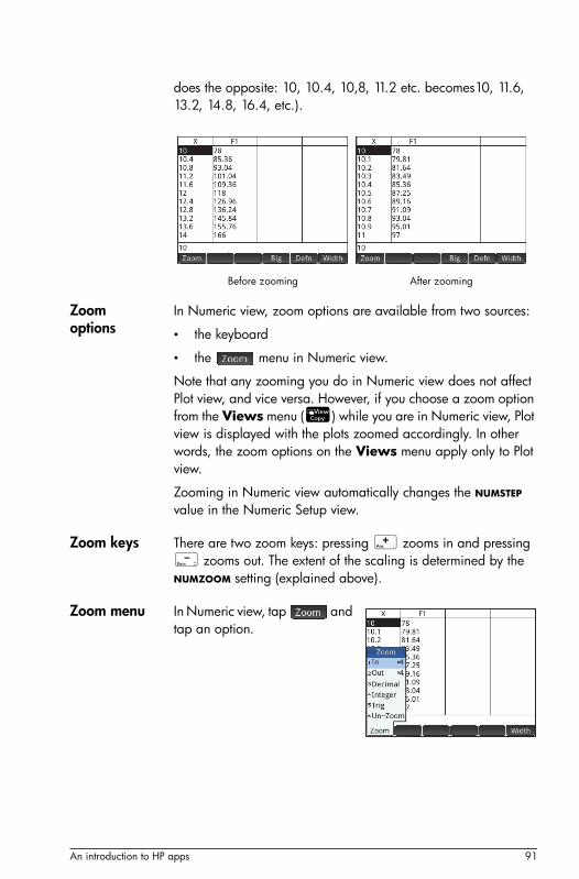
An introduction to HP apps 91
does the opposite: 10, 10.4, 10,8, 11.2 etc. becomes10, 11.6, 13.2, 14.8, 16.4, etc.).
Zoom options
In Numeric view, zoom options are available from two sources:
• the keyboard
• the menu in Numeric view.
Note that any zooming you do in Numeric view does not affect Plot view, and vice versa. However, if you choose a zoom option from the Views menu (V) while you are in Numeric view, Plot view is displayed with the plots zoomed accordingly. In other words, the zoom options on the Views menu apply only to Plot view.
Zooming in Numeric view automatically changes the NUMSTEP value in the Numeric Setup view.
Zoom keys There are two zoom keys: pressing + zooms in and pressing w zooms out. The extent of the scaling is determined by the NUMZOOM setting (explained above).
Zoom menu In Numeric view, tap and tap an option.
Before zooming After zooming

92 An introduction to HP apps
The zoom options are explained in the following table.
EvaluatingYou can step through the table of evaluations in Numeric view by pressing = or \. You can also quickly jump to an evaluation by entering the independent variable of interest in the independent variable column and tapping .
For example, suppose in the Symbolic view of the Function app, you have defined F1(X) as (X–1)2–3. Suppose further that you want to know what the value of that function is when X is 625.
1. Open Numeric view (M).
2. Anywhere in the independent column—the left-most column—enter 625.
Option Result
In The increment between consecutive values of the independent variable becomes the current value divided by the NUMZOOM setting. (Shortcut: press +.)
Out The increment between consecutive values of the independent variable becomes the current value multiplied by the NUMZOOM setting. (Shortcut: press w.)
Decimal Restores the default NUMSTART and NUMSTEP values: 0 and 0.1 respectively.
Integer The increment between consecutive values of the independent variable is set to 1.
Trig • If the angle measure setting is radians, sets the increment between consecutive values of the independent variable to /24 (approximately 0.1309).
• If the angle measure setting is degrees, sets the increment between consecutive values of the independent variable to 7.5.
Undo Zoom Returns the display to the previous zoom, or if there has been only one zoom, displays the graph with the original plot settings.

An introduction to HP apps 93
3. Tap .
Numeric view is refreshed, with the value you entered in the first row and the result of the evaluation in a cell to the right. In this example, the result is 389373.
Custom tablesIf you choose Automatic for the NUMTYPE setting, the table of evaluations in Numeric view will follow the settings in the Numeric Setup view. That is, the independent variable will start with the NUMSTART setting and increment by the NUMSTEP setting. (These settings are explained in “Common operations in Numeric Setup view” on page 95.) However, you can choose to build your own table where just the values you enter appear as independent variables.
1. Open Numeric Setup view.
SM
2. Choose BuildYourOwn from the NUMTYPE menu.
3. Open Numeric view.
Numeric view will be empty.
4. In the independent column—the left-most column—enter a value of interest.
5. Tap .
6. If you still have other values to evaluate, repeat from step 4.
Deleting data
To delete one row of data in your custom table, place the cursor in that row and press C.
To delete all the data in your custom table:
1. Press SJ.
2. Tap or press E to confirm your intention.

94 An introduction to HP apps
Numeric view: Summary of menu buttons
Button Purpose
To modify the increment between consecutive values of the independent variable in the table of evaluations. See page 90.
[BuildYourOwn only]
To edit the value in the selected cell.To overwrite the value in the selected cell, you can just start entering a new value without first tapping .Only visible if NUMTYPE is set to BuildYourOwn. See “Custom tables” on page 93.
[BuildYourOwn only]
To create a new row above the currently highlighted cell, with zero as the independent value. You can immediately start typing a new value. Only visible if NUMTYPE is set to BuildYourOwn. See “Custom tables” on page 93.
[BuildYourOwn only]
To sort the values in the selected column in ascending or descending order. Move the cursor to the column of interest, tap , select Ascending or Descending, and tap .Only visible if NUMTYPE is set to BuildYourOwn. See “Custom tables” on page 93.
Toggles the display between medium and large font.
Toggles between showing the value of the cell and the definition that generated the value.

An introduction to HP apps 95
Common operations in Numeric Setup view [Scope: Advanced Graphing, Function, Parametric, Polar, Sequence]
Press SM to open Numeric Setup view.
The Numeric Setup view is used to:
• set the starting number for the independent variable in automatic tables displayed in Numeric view: the NUMSTART field.
• set the increment between consecutive numbers in automatic tables displayed in Numeric view: the NUMSTEP field.
• specify whether the table of data to be displayed in Numeric view is to be based on the specified starting number and increment (automatic table) or to based on particular numbers for the independent variable that your specify (build-your-own table): the NUMTYPE field.
• set the zoom factor for zooming in or out on the table displayed in Numeric view: the NUMZOOM field.
Modifying Numeric Setup
Select the field you want to change and either specify a new value, or if you are choosing a type of table for Numeric view—automatic or build-your-own—choose the appropriate option from the NUMTYPE menu.
Displays a menu for you to choose to display the evaluations of 1, 2, 3, or 4 defintions. If you have more than four definitions seelcted in Symbolic view, you can press > to scroll rightwards and see more columns. Pressing < scrolls the columns leftwards.
Button Purpose (Cont.)

96 An introduction to HP apps
To help you set a starting number and increment that matches the current Plot view, tap .
Restore default settings
To restore one field to its default setting:
1. Select the field.
2. Press C.
To restore all default settings, press SJ.
Combining Plot and Numeric ViewsYou can display Plot view and Numeric view side-by-side. Moving the tracing cursor causes the table of values in Numeric view to scroll. You can also enter a value in the X column. The table scrolls to that value, and the tracing cursor jumps to the corresponding point on the selected plot.
To combine Plot and Numeric view in a split screen, press V and select Split Screen: Plot Table.
To return to Plot view, pressM. To return to Numeric view by pressing M.
Adding a note to an appYou can add a note to an app. Unlike general notes—those created via the Note Catalog: see chapter 25—an app note is not listed in the Note Catalog. It can only be accessed when the app is open.
An app note remains with the app if the app is sent to another calculator.
To add a note to an app:
1. Open the app.
An introduction to HP apps 97
2. Press SI (Info).
If a note has already been created for this app, its contents are displayed.
3. Tap and start writing (or editing) your note.
The format and bullet options available are the same as those in the Note Editor (described in “The Note Editor” on page 430).
4. To exit the note screen, press any key. Your note is automatically saved.
Creating an appThe apps that come with the HP Prime are built in and cannot be deleted. They are always available (simply by pressing I). However, you can create any number of customized instances of most apps. You can also create an instance of an app that is based on a previously customized app. Customized apps are opened from the application library in the same way that you open a built-in app.
The advantage of creating a customized instance of an app is that you can continue to use the built-in app for some other problem and return to the customized app at any time with all its data still in place. For example, you could create a customized version of the Sequence app that enables you to generate and explore the Fibonacci series. You could continue to use the built-in Sequence app to build and explore other sequences and return, as needed, to your special version of the Sequence app when you next want to explore the Fibonacci series. Or you could create a customized version of the Solve app—named, for example, Triangles—in which you set up, just once, the equations for solving common problems involving right-angled triangles (such as H=O/SIN(), A=H*COS(), O=A*TAN(), etc.). You could continue to use the Solve app to solve other types of problems but use your Triangle app to solve problems involving right-angled triangles. Just open Triangles, select which equation to use—you won’t need to re-enter them—enter the variables you know, and then solve for the unknown variable.
Like built-in apps, customized apps can be sent to another HP Prime calculator. This is explained in “Sharing data” on page 40.

98 An introduction to HP apps
Customized apps can also be reset, deleted, and sorted just as built-in apps can (as explained earlier in this chapter).
Note that the only apps that cannot be customized are the:
• Linear Explorer
• Quadratic Explorer and
• Trig Explorer apps.
Example Suppose you want to create a customized app that is based on the built-in Sequence app. The app will enable you to generate and explore the Fibonacci series.
1. Press I and use the cursor keys to highlight the Sequence app. Don’t open the app.
2. Tap . This enables you to create a copy of the built-in app and save it under a new name. Any data already in the built-in app is retained, and you can return to it later by opening the Sequence app.
3. In the Name field, enter a name for your new app—say, Fibonacci—and press E twice.
Your new app is added to the Application Library. Note that it has the same icon as the parent app—Sequence—but with the name you gave it: Fibonacci in this example.
4. If you want to clear the new app of any data that was in the parent app, make sure your new app is highlighted in the Application Library and tap . Tap when you are asked to confirm your intention.
Note that this step is entirely optional. If you want to keep building on data that was in the parent app, then don’t reset your new app.
5. You are now ready to use this app just as you would the built-in Sequence app. Tap on the icon of your new app to

An introduction to HP apps 99
open it. You will see in it all the same views and options as in the parent app.
In this example we have used the Fibonacci series as a potential topic for a customized app. To see how to create the Fibonacci series once inside the Sequence app—or an app based on the Sequence app—see chapter 16, “Sequence app”, beginning on page 257.
As well as cloning a built-in app—as described above—you can modify the internal workings of a customized app using the HP Prime programming language. See “Customizing an app” on page 460.
App functions and variablesFunctions App functions are used in HP apps to perform common
calculations. For example, in the Function app, the Plot view Fcn menu has a function called SLOPE that calculates the slope of a given function at a given point. The SLOPE function can also be used from the Home view or a program.
For example, suppose you want to find the derivative of x2 – 5 at x = 2. One way, using an app function, is as follows:
1. Press D.
2. Tap and select Function > SLOPE.
SLOPE() appears on the entry line, ready for you to specify the function and the x-value.
3. Enter the function:
Asjw5
4. Enter the parameter separator:
o
5. Enter the x-value and press E.
The slope (that is the derivative) at x = 2 is calculated: 4.
All the app functions are described in “App menu”, beginning on page 312.
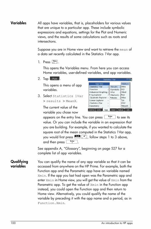
100 An introduction to HP apps
Variables All apps have variables, that is, placeholders for various values that are unique to a particular app. These include symbolic expressions and equations, settings for the Plot and Numeric views, and the results of some calculations such as roots and intersections.
Suppose you are in Home view and want to retrieve the mean of a data set recently calculated in the Statistics 1Var app.
1. Press a.
This opens the Variables menu. From here you can access Home variables, user-defined variables, and app variables.
2. Tap .
This opens a menu of app variables.
3. Select Statistics 1Var > results > MeanX.
The current value of the variable you chose now appears on the entry line. You can press E to see its value. Or you can include the variable in an expression that you are building. For example, if you wanted to calculate the square root of the mean computed in the Statistics 1Var app, you would first press Sj, follow steps 1 to 3 above, and then press E.
See appendix A, “Glossary”, beginning on page 527 for a complete list of app variables.
Qualifying variables
You can qualify the name of any app variable so that it can be accessed from anywhere on the HP Prime. For example, both the Function app and the Parametric app have an variable named Xmin. If the app you last had open was the Parametric app and enter Xmin in Home view, you will get the value of Xmin from the Parametric app. To get the value of Xmin in the Function app instead, you could open the Function app and then return to Home view. Alternatively, you could qualify the name of the variable by preceding it with the app name and a period, as in Function.Xmin.

An introduction to HP apps 101

102 An introduction to HP apps

Function app 103
5
Function app
The Function app enables you to explore up to 10 real-valued, rectangular functions of y in terms of x; for example, and .
Once you have defined a function you can:
• create graphs to find roots, intercepts, slope, signed area, and extrema, and
• create tables that show how functions are evaluated at particular values.
This chapter demonstrates the basic functionality of the Function app by stepping you through an example. More-complex functionality is described in chapter 4, “An introduction to HP apps”, beginning on page 59.
Getting started with the Function appThe Function app uses the customary app views: Symbolic, Plot and Numeric described in chapter 4.
For a description of the menu buttons available in this app, see:
• “Symbolic view: Summary of menu buttons” on page 76
• “Plot view: Summary of menu buttons” on page 86, and
• “Numeric view: Summary of menu buttons” on page 94.
Throughout this chapter, we will explore the linear function and the quadratic function .
y 1 x–= y x 1– 2 3–=
y 1 x–= y x 1– 2 3–=

104 Function app
Open the Function app
1. Open the Function app.
I Select Function
Recall that you can open an app just by tapping its icon. You can also open it by using the cursor keys to highlight it and then pressing E.
The Function app starts in Symbolic view. This is the defining view. It is where you symbolically define (that is, specify) the functions you want to explore.
The graphical and numerical data you see in Plot view and Numeric view are derived from the symbolic expressions defined here.
Define the expressions
There are 10 fields for defining functions. These are labelled F1(X) through F9(X) and F0(X).
2. Highlight the field you want to use, either by tapping on it or scrolling to it. If you are entering a new expression, just start typing. If you are editing an existing expression, tap and make your changes. When you have finished defining or changing the expression, press E.
3. Enter the linear function in F1(X).
1wdE
4. Enter the quadratic function in F2(X).
Rdw1>jw 3E
N O T E You can tap the button to assist in the entry of equations. In the Function app, it has the same effect as pressing d. (In other apps, d enters a different character.)

Function app 105
5. Decide if you want to:
– give one or more function a custom color when it is plotted
– evaluate a dependent function
– deselect a definition that you don’t want to explore
– incorporate variables, math commands and CAS commands in a definition.
For the sake of simplicity we can ignore these operations in this example. However, they can be useful and are described in detail in “Common operations in Symbolic view” on page 71.
Set up the plot
You can change the range of the x- and y-axes and the spacing of the tick marks along the axes
6. Display Plot Setup view.
SP (Setup)
For this example, you can leave the plot settings at their default values. If your settings do not match those in the illustration above, press SJ (Clear) to restore the default values.
See “Common operations in Plot Setup view” on page 86 for more information about setting the appearance of plots.
Plot the functions
7. Plot the functions.
P
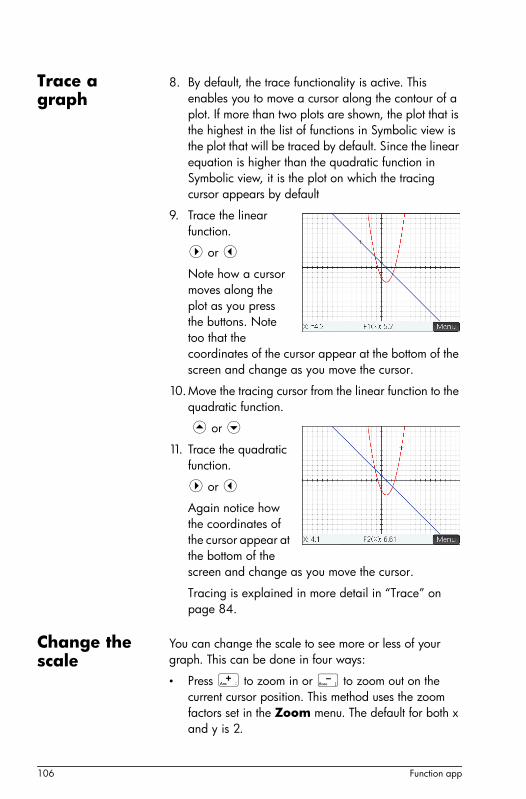
106 Function app
Trace a graph
8. By default, the trace functionality is active. This enables you to move a cursor along the contour of a plot. If more than two plots are shown, the plot that is the highest in the list of functions in Symbolic view is the plot that will be traced by default. Since the linear equation is higher than the quadratic function in Symbolic view, it is the plot on which the tracing cursor appears by default
9. Trace the linear function.
> or <
Note how a cursor moves along the plot as you press the buttons. Note too that the coordinates of the cursor appear at the bottom of the screen and change as you move the cursor.
10.Move the tracing cursor from the linear function to the quadratic function.
= or \
11. Trace the quadratic function.
> or <
Again notice how the coordinates of the cursor appear at the bottom of the screen and change as you move the cursor.
Tracing is explained in more detail in “Trace” on page 84.
Change the scale
You can change the scale to see more or less of your graph. This can be done in four ways:
• Press + to zoom in or w to zoom out on the current cursor position. This method uses the zoom factors set in the Zoom menu. The default for both x and y is 2.

Function app 107
• Use the Plot Setup view to specify the exact x-range (XRNG) and y-range (YRNG) you want.
• Use options on the Zoom menu to zoom in or out, horizontally or vertically, or both, etc.
• Use options on the View menu (V) to select a pre-defined view. Note that the Autoscale option attempts to provide a best fit, showing as many of the critical features of each plot as possible.
N O T E By dragging a finger horizontally or vertically across the screen, you can quickly see parts of the plot that are initially outside the set x and y ranges. This is easier than resetting the range of an axis.
Zoom options—with numerous examples—are explained in more detail in “Zoom” on page 78.
Display Numeric view
12. Display the Numeric view:
M
The Numeric view displays data generated by the expressions you defined in Symbolic view. For each expression selected in Symbolic view, Numeric view displays the value that results when the expression is evaluated for various x-values.
Set up Numeric view
13. Display the Numeric Setup view:
SM(Setup)
You can set the starting value and step value (that is, the increment) for the x-column, as well as the zoom factor for zooming in or out on a row of the table. Note that in Numeric view, zooming does not affect the size of what is displayed. Instead, it changes the Num Step setting (that is, the increment between consecutive x-values). Zooming in

108 Function app
decreases the increment; zooming out increases the increment. This is further explained in “Zoom” on page 90.
You can also choose whether the table of data in Numeric view is automatically populated or whether it is populated by you typing in the particular x-values you are interested in. These options—Automatic or BuildYourOwn—are available from the Num Type list. They are explained in detail in “Custom tables” on page 93.
14. Press SJ(Clear) to reset all the settings to their defaults.
15. Make the Numeric view settings match the axes range in Plot view:
Tap .For example, if you have zoomed in on the plot in Plot view so that the visible x-range is now –4 to 4, this option will set NUMSTART to –4.
Explore Numeric view
16. Re-display Numeric view:
M
To navigate around a table
17. Using the cursor keys, scroll through the values in the independent column (column X). Note that the values in the F1 and F2 columns match what you would get if you substituted the values in the X column for x in the

Function app 109
expressions selected in Symbolic view: 1–x and (x–1)2–3. You can also scroll through the columns of the dependant variables (labeled F1 and F2 in the illustration above).
To go directly to a value
18. Place the cursor is in the X column and type the desired value. For example, to jump straight to the row where x = 10:
1 0
To access the zoom options
Numerous zoom options are available by tapping . These are explained in “Zoom” on page 90.
A quick way to zoom in (or zoom out) is to press + (or w). This zooms in (or out) by the Num Zoom value set in the Numeric Setup view (see page 107). The default value is 4. Thus if the current increment (that is, the Num Step value) is 0.4, zooming in will further divide that interval by four smaller intervals. So instead of x-values of 10, 10.4, 10,8, 11.2 etc., the x-values will be 10, 10.1, 10.2, 10.3, 10.4, etc. (Zooming out does the opposite: 10, 10.4, 10,8, 11.2 etc. becomes10, 11.6, 13.2, 14.8, 16.4, etc.)
Other options As explained on page page 94, you can also:
• change the size of the font from medium to large
• display the definition responsible for generating a column of values
• choose to show 1, 2, 3, or 4 columns of data.
You can also combine Plot and Numeric view. See “Custom tables” on page 93.
Analyzing functionsThe Function menu ( ) in Plot view enables you to find roots, intersections, slopes, signed areas, and extrema for any function defined in the Function app. If

110 Function app
you have more than one function plotted, you may need to choose the function of interest beforehand.
Display the Plot view menu
The Function menu is a sub-menu of the Plot view menu. First, display the Plot view menu:
P
To find a root of the quadratic function
Suppose you want to find the root of the quadratic equation defined earlier. Since a quadratic equation can have more than one root, you will need to move the cursor closer to the root you are interested in than to any other root. In this example, you will find the root of the quadratic close to where x = 3.
1. If it is not already selected, select the quadratic equation:
=or\
2. Press >or< to move the cursor near to where x = 3.
3. Tap and select Root
The root is displayed at the bottom of the screen.
If you now move the trace cursor close to x = –1 (the other place where the quadratic crosses the x-axis) and selected Root gain, the other toot is displayed.

Function app 111
Note the button. If you tap this, one or two dotted lines pick out the point of interest (in this case a root). If, while this button is active, you tap elsewhere on the screen, a set of dotted lines appears on the screen. The dotted lines intersect the currently selected plot closest to the point you tapped. Their point of intersection is a tracing cursor. If you make another calculation where there is more than one answer, the answer that applies to the point closest to this tracing cursor is the answer provided. This is a faster way of choosing a point of interest than using the trace cursor. (You can move this tracing cursor using the cursor keys if you need finer precision.)
To find an intersection of the two functions
Just as there are two roots of the quadratic equation, there are two points at which both functions intersect. As with roots, you need to position your cursor closer to the point you are interested in. In this example, the intersection close to x = 1 will be determined.
The Go To command is another way of moving the trace cursor to a particular point.
1. Tap to re-display the menu, tap , enter Q1, and tap .
The tracing cursor will now be on one of the functions at x = 1.
2. Tap and select Intersection.
A list appears giving you a choice of functions and axes.
3. Choose the function whose point of intersection with the currently selected function you wish to find.

112 Function app
The coordinates of the intersection are displayed at the bottom of the screen.
Tap on the screen near the other intersection, and repeat from step 2. The coordinates of the intersection nearest to where you tapped are displayed at the bottom of the screen.
To find the slope of the quadratic function
We will now find the slope of the quadratic function at the intersection point.
1. Tap to re-display the menu, tap and select Slope.
The slope (that is, the gradient) of the function at the intersection point is displayed at the bottom of the screen.
You can press < or > to trace along the curve and see the slope at other points. You can also press = or \ to jump to another function and see the slope at points on it.
2. Press to re-display the Plot menu.
To find the signed area between the two functions
We’ll now find the area between the two functions in the range .
1. Tap and select Signed area.
2. Specify the start value for x:
Tap and press Q1.3E.
3. Tap .
1.3– x 2.3

Function app 113
4. Select the other function as the boundary for the integral. (If F1(X) is the currently selected function, you would choose F2(X) here, and vice versa.)
5. Specify the end value for x:
Tap and press 2.3E.
The cursor jumps to x = 2.3 and the area between the two functions is shaded.
6. To display the numerical value of the integral, tap
.7. Tap to return
to the Plot menu.
Shortcut: When the Goto option is available, you can display the Go To screen simply by typing a number. The number you type appears on the entry line. Just tap to accept it.
To find the extremum of the quadratic
1. To calculate the coordinates of the extremum of the quadratic equation, move the tracing cursor near to it (if necessary), tap
and select Extremum.

114 Function app
The coordinates of the extremum are displayed at the bottom of the screen.
N O T E The ROOT INTERSECTION, and EXTREMUM operations return only one value even if the function in question has more than one root, intersection, or extremum. The app will only return values that are closest to the cursor. You will need to move the cursor closer to other roots, intersections, or extrema if you want the app to calculate values for those.
The Function VariablesThe result of each numerical analysis in the Function app is assigned to a variable. These variables are named:
• Root
• Isect (for Intersection)
• Slope
• SignedArea
• Extremum
The result of each new analysis overwrites the previous result. For example, if you find the second root of a quadratic equation after finding the first, the value of Root changes form the first to the second root.
To access Function variables
The Function variables are available in Home view and in the CAS, where they can be included as arguments in calculations. They are also available in Symbolic view.
1. To access the variables, press a, tap and select Function.
2. Select Results and then the variable of interest.
The variable’s name is copied to the insertion point and its value is used in evaluating the expression that contains it.

Function app 115
For example, in Home view or the CAS you could select SignedArea from the Vars menus, press s3E and get the current value of SignedArea multiplied by three.
Function variables can also be made part of a function’s definition in Symbolic view. For example, you could define a function as x2–x–Root.
The full range of variables, and their use in calculations, is covered in detail in chapter 21, “Variables”, beginning on page 373.

116 Function app
Summary of FCN operations
Operation Description
Root Select Root to find the root of the current function nearest to the tracing cursor. If no root is found, but only an extremum, then the result is labeled Extremum instead of Root. The cursor is moved to the root value on the x-axis and the resulting x-value is saved in a variable named Root.
Extremum Select Extremum to find the maximum or minimum of the current function nearest to the tracing cursor. The cursor moves to the extremum and the coordinate values are displayed. The resulting value is saved in a variable named Extremum.
Slope Select Slope to find the numeric derivative of the current function at the current position of the tracing cursor. The result is saved in a variable named Slope.
Signed area Select Signed area to find the numeric integral. (If there are two or more expressions checkmarked, then you will be asked to choose the second expression from a list that includes the x-axis.) Select a starting point and an ending point. The result is saved in a variable named SignedArea.
Intersec-tion
Select Intersection to find the intersection of the graph you are currently tracing and another graph. You need to have at least two selected expressions in Symbolic view. Finds the intersection closest to the tracing cursor. Displays the coordinate values and moves the cursor to the intersection. The resulting x-value is saved in a variable named Isect.

Advanced Graphing app 117
6
Advanced Graphing app
The Advanced Graphing app enables you to define and explore the graphs of symbolic open sentences in x, y, both or neither. You can plot conic sections, polynomials in standard or general form, inequalities, and functions. The following are examples of the sorts of open sentences you can plot:
1. x2/3 – y2/5 = 1
2. 2x – 3y ≤ 6
3. y MOD x = 3
4.
5. x2 + 4x = –4
6. 1 < 0
The illustrations below show what these open sentences look like when plotted:
x2 y2+ 5– 2
sin 8yx----
atan sin>
Example 1 Example 2

118 Advanced Graphing app
Getting started with the Advanced Graphing appThe Advanced Graphing app uses the customary app views: Symbolic, Plot, and Numeric described in chapter 4.
For a description of the menu buttons available in this app, see:
• “Symbolic view: Summary of menu buttons” on page 76
• “Plot view: Summary of menu buttons” on page 86, and
• “Numeric view: Summary of menu buttons” on page 94.
The Trace option in the Advanced Graphing app works differently than in other apps and is described in detail in this chapter.
In this chapter, we will explore the rotated conic defined by:
Example 3 Example 4
Example 5 Example 6
x2
2---- 7xy
10---------–
3y2
4------- x
10------–
y5--- 10–+ + 0

Advanced Graphing app 119
Open the app
1. Open the Advanced Graphing app:
I Select Advanced Graphing
The app opens in the Symbolic view.
Define the open sentence
2. Define the open sentence:
j n 2 > w 7 n 10 > + 3
j n 4 > w n 10 > + n 5 >w 10 < 0 E
Note that < can be easily selected from the relations palette: Sv.
3. Decide if you want to:
– give one or more open sentence a custom color when it is plotted
– evaluate a dependent function
– deselect a definition that you don’t want to explore
– incorporate variables, math commands and CAS commands in a definition.
For the sake of simplicity we can ignore these operations in this example. However, they can be useful and are described in detail in “Common operations in Symbolic view” on page 71.
Set up the plot
You can change the range of the x- and y-axes and the spacing of the interval marks along the axes.

120 Advanced Graphing app
4. Display Plot Setup view:
SP (Setup)
For this example, you can leave the plot settings at their default values. If your settings do not match those in the illustration at the right example, press SJ (Clear) to restore the default values.
See “Common operations in Plot Setup view” on page 86 for more information about setting the appearance of plots.
Plot the selected definitions
5. Plot the selected definitions:
P
Explore the graph
6. Display the Plot view menu items:
Note that you have otions to zoom, trace, go to a specified x- or y- value, and display the definition of the selected graph.You can use the zoom and split screen functionality discussed in chapter 5.
A special feature of the Advanced Graphing app enables you to edit the definition of a graph from within the Plot view.

Advanced Graphing app 121
7. Tap . The definition as you entered it in Symbolic view appears at the bottom of the screen.
8. Tap .
The definition is now editable.
9. Change the < to = and tap .
Notice that the graph changes to match the new definition. The definition in Symbolic view also changes.
10.Tap to drop the definition to the bottom of the screen so that you can see the full graph. The definition is converted from textbook mode to algebraic mode to save screen space.
Trace a graph
[This functionality is not available as of build 3015]
Display the Numeric view
11.Press M to display the Numeric view.
Unlike in many other apps, the Numeric view in the Advanced Graphing app does not give a table of values generated by the definitions selected in Symbolic view. Instead, for various combinations of x and y, Numeric view shows whether the open sentence is satisfied.
Explore Numeric view
12. With the cursor in the X column, type a new value and tap .The table scrolls to the value you entered.
You can also enter a value in the Y column and tap . Press < and > to move between the columns
in Numeric view.

122 Advanced Graphing app
You can also zoom in or out on the X variable or Y variable (thereby decreasing or increasing the increment between consecutive values). This and other options are explained in “Common operations in Numeric view” on page 90.
Set up Numeric view
13. Display the Numeric Setup view:
SM(Setup)
You can set the starting value and step value (that is, the increment) for both the X-column and the Y-column, as well as the zoom factor for zooming in or out on a row of the table. Note that in Numeric view, zooming does not affect the size of what is displayed. Instead, it changes the Num Step setting (that is, the increment between consecutive x-values). Zooming in decreases the increment; zooming out increases the increment. This is further explained in “Zoom” on page 90.
You can also choose whether the table of data in Numeric view is automatically populated or whether it is populated by you typing in the particular x-values and x-values you are interested in. These options—Automatic or BuildYourOwn—are available from the Num Type list. They are explained in detail in “Custom tables” on page 93.
To make the Numeric view settings match the axes range in Plot view, tap .

Geometry 123
7
Geometry
The Geometry app enables you to draw and explore geometric constructions. A geometric construction can be composed of any number of geometric objects, such as points, lines, polygons, curves, tangents, and so on. You can take measurements (such as areas and distances), manipulate objects, and note how measurements change.
There are five app views:
• Plot view: provides drawing tools for you to construct geometric objects
• Symbolic view: provides editable definitions of the objects in Plot view
• Numeric view: for making calculations about the objects in Plot view
• Plot Setup view: for customizing the appearance of Plot view
• Symbolic Setup view: for overriding certain system-wide settings
There is no Numeric Setup view in this app.
To open the Geometry app, press I and select Geometry. The app opens in Plot view.
Getting started with the Geometry appThe following example shows how you can graphically represent the derivative of a curve, and have the value of the derivative automatically update as you move a point of tangency along the curve. The curve to be explored is y = 3sin(x).
Since the accuracy of our calculation in this example is not too important, we will first change the number format to fixed at 3 decimal places. This will also help keep our geometry workspace uncluttered.

124 Geometry
Preparation 1. Press SH.
2. On the Home Setting screen set the number format to Fixed and the number of decimal places to 3.
Open the app and plot the graph
3. Press I and select Geometry.
If there are objects showing that you don’t need, press SJ and confirm your intention by tapping .
4. Select the type of graph you want to plot. In this example we are plotting a simple sinusoidal function, so choose:
> Plot > Function
5. With plotfunc( on the entry line, enter 3*sin(x):
3seASsE
Note that x must be entered in lowercase in the Geometry app.
If your graph doesn’t resemble the illustration at the right, adjust the X Rng and Y Rng values in Plot Setup view (SP).
We’ll now add a point to the curve, a point that will be constrained always to follow the contour of the curve.
Add a constrained point
6. Tap and select Point On.
Choosing Point On rather than Point means that the point will be constrained to whatever it is placed on.
7. Tap anywhere on the graph, press E and then press J.
Notice that a point is added to the graph and given a name (B in this example). Tap a blank area of the screen to deselect everything. (Objects colored cyan are selected.)
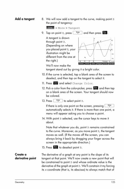
Geometry 125
Add a tangent 8. We will now add a tangent to the curve, making point B the point of tangency:
> More > Tangent
9. Tap on point B, press E and then press J.
A tangent is drawn through point B. (Depending on where you placed point B, your illustration might be different from the one at the right.)
We’ll now make the tangent stand out by giving it a bright color.
10. If the curve is selected, tap a blank area of the screen to deselect, and then tap on the tangent to select it.
11. Press Z and select Change Color.
12. Pick a color from the color-picker, press J and then tap on a blank area of the screen. Your tangent should now be colored.
13. Press E to select point B.
If there is only one point on the screen, pressing E automatically selects it. If there is more than one point, a menu will appear asking you to choose a point.
14. With point B selected, use the cursor keys to move it about.
Note that whatever you do, point B remains constrained to the curve. Moreover, as you move point B, the tangent moves as well. (If the moves off the screen, you can always bring it back by dragging your finger across the screen in the appropriate direction.)
15. Press J to deselect point B.
Create a derivative point
The derivative of a graph at any point is the slope of its tangent at that point. We’ll now create a new point that will be constrained to point B and whose ordinate value is the derivative of the graph at point B. We’ll constrain it my forcing its x coordinate (that is, its abscissa) to always match that of

126 Geometry
point B, and its y coordinate (that is, its ordinate) to always equal the slope of the derivative at that point.
16. To define a point in terms of the attributes of other geometric objects, you need to go to Symbolic view:
Y
Note that each object you have so far created is listed in Symbolic view. Note too that the name for an object in Symbolic view is the name it was given in Plot view but prefixed with a “G”. Thus the graph—labeled A in Plot view—is labeled GA in Symbolic view.
17. Highlight GC and tap .
When creating objects that are dependent on other objects, the order in which they appear in Symbolic view is important. Objects are drawn in Plot view in the order in which they appear in Symbolic view. Since we are about to create a new point that is dependent on the attributes of GB and GC, it is important that we place its definition after that of both GB and GC. That is why we made sure we were at the bottom the list of definitions before tapping . If our new definition appeared higher up in Symbolic view, the point we are about to create wouldn’t be drawn in Plot view.
18. Tap and choose Point > point
You now need to specify the x and y coordinates of the new point. The former is to be constrained to abscissa of point B (referred to as GB in Symbolic view) and the later is to constrained to the slope of C (referred to as GC in Symbolic view).
19. You should have point() on the entry line. Between the parentheses, add:
abscissa(GB),slope(GC)
You can enter the commands by hand, or choose them from the Catlg menu (one of the five Toolbox menus).

Geometry 127
20.Tap .
The definition of your new point is added to Symbolic view. When you return to Plot view, you will see a point named D and it will have the same x coordinate as point B.
21. Press P.
If you can’t see point D, pan until it comes into view. The y coordinate of D will be the derivative of the curve at point B.
Since its difficult to read coordinates off the screen, we’ll add a calculation that will give the exact derivative (to three decimal places) and which we can display in Plot view.
Add some calculations
22. Press M.
Numeric view is where you enter calculations.
23.Tap .
24.Tap and choose Measure > slope
25.Between parentheses, add the name of the tangent, namely GC, and tap .
Notice that the current slope is calculated and displayed. The value here is dynamic, that is, if the slope of the tangent changes in Plot view, the value of the slope is automatically updated in Numeric view.
26.With the new calculation highlighted in Numeric view, tap .
Selecting a calculation in Numeric view means that it will also be displayed in Plot view.

128 Geometry
27. Press P to return to Plot view.
Notice the calculation that you have just created in Numeric view is displayed at the top left of the screen.
Let’s now add two more calculations to Numeric view and have them displayed in Plot view.
28.Press M to return to Numeric view.
29. Tap , enter GB, and tap .
Entering just the name of a point will show its coordinates.
30.Tap , enter GC, and tap .
Entering just the name of a line will show its equation.
31. Make sure both of these new equations are selected (by choosing each one and pressing ).
32. Press P to return to Plot view.
Notice that your new calculations are displayed.
33.Press E and choose point GB.
34.Use the cursor keys to move point B along the graph. Note that with each move, the results of the calculations shown at the top left of the screen change.
Trace the derivative
Point D is the point whose ordinate value matches the derivative of the curve at point B. It is easier to see how the derivative changes by looking at a plot of it rather than comparing subsequent calculations. We can do that by tracing point D as it moves in response to movements of point B.
First we’ll hide the calculations so that we can better see the trace curve.

Geometry 129
35.Press M to return to Numeric view.
36.Select each calculation in turn and tap . All calculations should now be deselected.
37. Press P to return to Plot view.
38.Press E and select point GD.
39. Tap and select More > Trace
40.Press E and select point GB.
41. Using the cursor keys, move B along the curve. You will notice that a shadow curve is traced out as you move B. This is the curve of the derivative of 3sin(x).
Plot view in detailIn Plot view you can directly draw objects on the screen using various drawing tools. For example, For example, to draw a circle, tap and select Circle. Now tap where you want the center of the circle to be and press E. Next, tap a point that is to be on the circumference and press E. A circle is drawn with a center at the location of your first tap, and with a radius equal to the distance between your first tap and second tap.
Creating or selecting an object always involves at least two steps: tap and press E. Only by pressing E do you confirm your intention to create the point or select an object. When creating a point, you can tap on the screen and then use the cursor keys to accurately position the point before pressing E.
Note that there are on-screen instructions to help you. For example, Hit Center means tap where you want the center
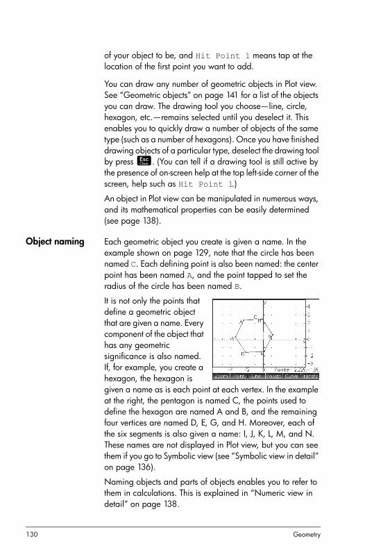
130 Geometry
of your object to be, and Hit Point 1 means tap at the location of the first point you want to add.
You can draw any number of geometric objects in Plot view. See “Geometric objects” on page 141 for a list of the objects you can draw. The drawing tool you choose—line, circle, hexagon, etc.—remains selected until you deselect it. This enables you to quickly draw a number of objects of the same type (such as a number of hexagons). Once you have finished drawing objects of a particular type, deselect the drawing tool by press J. (You can tell if a drawing tool is still active by the presence of on-screen help at the top left-side corner of the screen, help such as Hit Point 1.)
An object in Plot view can be manipulated in numerous ways, and its mathematical properties can be easily determined (see page 138).
Object naming Each geometric object you create is given a name. In the example shown on page 129, note that the circle has been named C. Each defining point is also been named: the center point has been named A, and the point tapped to set the radius of the circle has been named B.
It is not only the points that define a geometric object that are given a name. Every component of the object that has any geometric significance is also named. If, for example, you create a hexagon, the hexagon is given a name as is each point at each vertex. In the example at the right, the pentagon is named C, the points used to define the hexagon are named A and B, and the remaining four vertices are named D, E, G, and H. Moreover, each of the six segments is also given a name: I, J, K, L, M, and N. These names are not displayed in Plot view, but you can see them if you go to Symbolic view (see “Symbolic view in detail” on page 136).
Naming objects and parts of objects enables you to refer to them in calculations. This is explained in “Numeric view in detail” on page 138.

Geometry 131
You can rename an object. See “Renaming an object” on page 137.
Selecting an object
To select an object, just tap on it. The color of a selected item changes to cyan.
To select a point in Plot view, just press E. A list of all the points appears. Select the one you want.
Hiding names You can choose to hide the name of an object in Plot view:
1. Press Z.
2. Select Toggle Caption.
The Select Object menu appears.
3. Select the object whose label (that is, caption) you want to hide.
4. Press J.
Redisplay a hidden name by repeating this procedure.
Moving objects Points To move a point press E. A list of all the points appears. Select the one you want to move, then tap on the new location for it, and press E. You can also press the arrow keys to move a selected point. A point can be selected directly by tapping on it. (If the bottom-right of the screen shows the name of the point, you have accurately tapped the point; otherwise the pointer coordinates are shown, indicating that the point is not selected.)
Composite objects To move a multi-point object, see “Translation” on page 148.
Coloring objects An object is colored black by default (and cyan when it is selected). If you want to change the color of an object:
1. Press Z.
2. Select Change Color.
The Select Object menu appears.
3. Select the object whose color you want to change.
The Choose Color palette appears.
4. Select the color you want.
5. Press J.

132 Geometry
Note that for object with closed contours (such as a circle or polygon) it is the fill color that is changed.
Filling objects An object with closed contours (such as a circle or polygon) can be filled with color.
1. Press Z.
2. Select Fill with Color.
The Select Object menu appears.
3. Select the object you want to fill.
The object is highlighted.
1. Press Z.
2. Select Change Color.
The Choose Color palette appears.
3. Select the color you want.
4. Press J.
Removing fill To remove the fill from an object:
1. Press Z.
2. Select Fill with Color.
The Select Object menu appears.
3. Select the object.
Undoing You can undo your last addition or change to Plot view by pressing t. However, you must have keyboard shortcuts activated for this to work. See page 135.
Clearing an object
To clear one object, select it and tap C. Note that an object is distinct from the points you entered to create it. Thus deleting the object does not delete the points that define it. Those points remain in the app. For example, if you select a circle and press C, the circle is deleted but the center point and radius point remain.

Geometry 133
If you tap C when no object is selected, a list of objects appears. Tap on the one you want to delete, and tap to confirm your intention. If you don’t want to delete an object, press J to close the list.
Note that points you add to an object once the object has been defined are cleared when you clear the object. Thus if you place a point (say D) on a circle and delete the circle, the circle and D are deleted, but the defining points—the center and radius points—remain.
Clearing all objects
To clear the app of all geometric objects, press SJ. You will be asked to confirm your intention to do so. Tap to clear the app, or to keep the app as it is,
Moving about the Plot view
You can pan by dragging a finger across the screen: either up, down, left, or right. You can also use the cursor keys to pan once the cursor is at the edge of the screen.
Zooming You can zoom using touch gestures (see page 3) or by tapping and choosing a zoom option. The zoom options are the same as you find in the Plot view of many apps in the calculator (see “Zoom” on page 78).
Plot view: buttons and keys
Button or key
Purpose
Various scaling options. See “Zoom” on page 78.
Tools for creating various types of points. See “Points” on page 141
Tools for creating various types of lines. See “Line” on page 143
Tools for creating various types of polygons. See “Polygon” on page 145

134 Geometry
Plot Setup viewThe Plot Set view enables you to configure the appearance of Plot view and to take advantage of keyboard shortcuts.The fields and options are:
• X Rng: Two fields for entering the minimum and maximum x-values, thereby giving the default horizontal range. As well as changing this range on the Geometry Plot Setup screen, you can change it by panning and zooming.
• Y Rng: Two fields for entering the minimum and maximum y-values, thereby giving the default vertical range. As well as changing this range on the Geometry Plot Setup screen, you can change it by panning and zooming.
• Axes: A toggle option to hide (or reshow) the axes in Plot view.
Keyboard shortcut: a
Tools for creating various types of curves and plots. See “Curve” on page 146
Tools for geometric transformations of vari-ous kinds. See “Geometric transformations” on page 148.
C Deletes a selected object (or the character to the left of the cursor if the entry line is active).
J De-activate the current drawing tool
SJ Clears the Plot view of all geometric objects.
Shortcut keys To quickly add an object, and undo what you’ve done. See page 135.
Button or key
Purpose (Continued)

Geometry 135
• Labels: A toggle option to hide (or reshow) the names of the geometric objects (A, B, C, etc.) in Plot view.
• Function Labels: A toggle option to hide (or reshow) the expression that generated a plot with the plot. These should not be confused with calculation labels. You can show function labels without also showing calculation labels and vice versa).
• Shortcuts: A toggle option to enable (or disable) keyboard shortcuts (that is, hot keys) in Plot view. With this option enabled, the following shortcuts become available:
Key Result in Plot view
a Hide (or reshow) the axes.
F Selects the circle drawing tool. Follow the instructions on the screen (or see page 146).
c Erases all trace lines (see page 142)
g Selects the intersection drawing tool. Fol-low the instructions on the screen (or see page 142).
j Selects the line drawing tool. Follow the instructions on the screen (or see page 143).
B Selects the point drawing tool. Follow the instructions on the screen (or see page 141).
r Selects the segment drawing tool. Follow the instructions on the screen (or see page 143).
n Selects the triangle drawing tool. Follow the instructions on the screen (or see page 145).
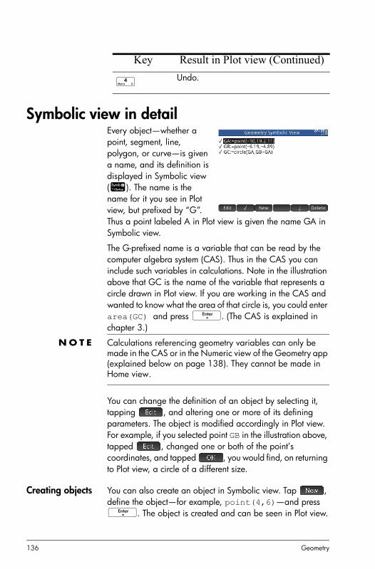
136 Geometry
Symbolic view in detailEvery object—whether a point, segment, line, polygon, or curve—is given a name, and its definition is displayed in Symbolic view (Y). The name is the name for it you see in Plot view, but prefixed by “G”. Thus a point labeled A in Plot view is given the name GA in Symbolic view.
The G-prefixed name is a variable that can be read by the computer algebra system (CAS). Thus in the CAS you can include such variables in calculations. Note in the illustration above that GC is the name of the variable that represents a circle drawn in Plot view. If you are working in the CAS and wanted to know what the area of that circle is, you could enter area(GC) and press E. (The CAS is explained in chapter 3.)
N O T E Calculations referencing geometry variables can only be made in the CAS or in the Numeric view of the Geometry app (explained below on page 138). They cannot be made in Home view.
You can change the definition of an object by selecting it, tapping , and altering one or more of its defining parameters. The object is modified accordingly in Plot view. For example, if you selected point GB in the illustration above, tapped , changed one or both of the point’s coordinates, and tapped , you would find, on returning to Plot view, a circle of a different size.
Creating objects You can also create an object in Symbolic view. Tap , define the object—for example, point(4,6)—and press E. The object is created and can be seen in Plot view.
t Undo.
Key Result in Plot view (Continued)

Geometry 137
Another example: to draw aline through points P and Q, enter line(GP,GQ) in Symbolic view and press E. When you return to Plot view, you will see a line passing through points P and Q.
The object-creation commands available in Symbolic view can be seen by tapping . The syntax for each command is given in “Geometry functions and commands” on page 151
Re-ordering entries
You can re-order the entries in Symbolic view. Objects are drawn in Plot view in the order in which they are defined in Symbolic view. To change the position of an entry, highlight it and tap either (to move it down the list) or (to move it up).
Hiding an object To prevent an object displaying in Plot view, deselect it in Symbolic view:
1. Highlight the item to be hidden.
2. Tap .
Repeat the procedure to make the object visible again.
Deleting an object
As well as deleting an object in Plot view (see page 132) you can delete an object in Symbolic view.
1. Highlight the definition of the object you want to delete.
2. Tap or press C.
To delete all objects, press SJ.
Renaming an object
You can change the name that is automatically given to an object. For example, you could rename a circle from GC to GCircle, or rename one square from GJ to GHouse and another from GL to GPaddock. The new names will also appear in Plot view (and can also be referenced in Numeric view and in the CAS).

138 Geometry
Note that a name must be a single string of characters (that is, it must contain no spaces). Also, the G prefix must be retained.
1. Highlight the definition of the object you want to rename.
2. Tap .
3. Make your change and tap . [Functionality removed as at 3015]
Symbolic Setup viewThe Symbolic view of the Geometry app is common with many apps. It is used to override certain some system-wide settings. For details, see “Symbolic Setup view” on page 64.
Numeric view in detail Numeric view (M) enables you to do calculations in the Geometry app. The results displayed are dynamic—if you manipulate an object in Plot view or Symbolic view, any calculations in Numeric view that refer to that object are automatically updated to reflect the new properties of that object.
Consider circle C in the illustration at the right. To calculate the area and radius of C:
1. Press M to open Numeric view.
2. Tap .
3. Tap and choose Measure > Area.
Note that area() appears on the entry line, ready fro you specify the object whose area you are interested in.
All the Geometry commands are explained in “Geometry functions and commands” on page 151.

Geometry 139
4. Tap , choose Curves and then the curve whose area you are interested in.
The name of the object is placed between the parentheses.
You could have entered the command and object name manually, that is, without choosing them from menus. If you enter object names manually, remember that the name of the object in Plot view must be given a “G” prefix if it is used in any calculation. Thus the circle named C in Plot view must be referred to as GC in Numeric view and Symbolic view.
5. Press E or tap . The area is displayed.
6. Tap .
7. Enter radius(GC) and tap . The radius is displayed.
Note that the syntax used here is the same as you use in the CAS to calculate the properties of geometric objects.
The Geometry functions and their syntax are described in “Geometry functions and commands” on page 151.
8. Press P to go back to Plot view. Now manipulate the circle is some way that changes its area and radius. For example, select the center point (A) and use the cursor keys to move it to a new location. (Remember to press E when you have finished.)
9. Press M to go back to Numeric view. Notice that the area and radius calculations have been automatically updated.
N O T E If an entry in Numeric view is too long for the screen, you can press > to scroll the rest of the entry into view. Press < to scroll back to the original view.

140 Geometry
Listing all objects
When you are creating a new calculation in Numeric view, the menu item appears. Tapping gives you a list of all the objects in your Geometry workspace. These are also grouped according to their type, with each group given its own menu.
If you are building a calculation, you can select an object from one of these variables menus. The name of the selected object is placed at the insertion point on the entry line.
Getting object properties
As well as employing functions to make calculations in Numeric view, you can also get various parameters of objects just by tapping specifying the object’s name. For example, you can get the exact coordinates of a point by entering the point and pressing E. Another example: if you can get the formula for a line just by entering its name, or the center point and radious of a circle just by entering the name of the circle.
Displaying calculations in Plot view
To have a calculation made in Numeric view appear in Plot view, just highlight it in Numeric view and tap
. A checkmark appears beside the calculation.
Repeat the procedure to prevent the calculation being displayed in Plot view. The checkmark is cleared.
Editing a calculation
1. Highlight the calculation you want to delete.
2. Tap .
3. Make your change and tap .
Deleting a calculation
1. Highlight the calculation you want to delete.
2. Tap .

Geometry 141
To delete all calculations, press SJ. Note that deleting a calculation does not delete any objects from Plot or Symbolic view.
Geometric objectsThe geometric objects discussed in this section are those that can be created in Plot view. Objects can also be created in Symbolic view—more, in fact, than in Plot view—but these are discussed in “Geometry functions and commands” on page 151.
In Plot view, you choose a drawing tool to draw an object. The tools are listed in this section. Note that once you select a drawing tool, it remains selected until you deselect it. This enables you to quickly draw a number of objects of the same type (such as a number of circles). To deselect the current drawing tool, press J. (You can tell if a drawing tool is still active by the presence of on-screen help in the top left-side corner of the screen, help such as Hit Point 1.)
The steps provided in this section are based on touch entry. For example, to add a point, the steps will tell you to tap on the screen where you want the point to be. However, you can also use the cursor keys to position the cursor where you want the point to be and then press E.
The drawing tools for the geometric objects listed in this section can be selected from the menu buttons a the bottom of the screen. Some objects can also be entered using a keyboard shortcut. For example, you can select the triangle drawing tool by pressing n. (Keyboard shortcuts are only available if they ave been turned on in Plot Setup view. See page 134.)
Points Tap to display a menu and submenus of options for entering various types of points. The menus and submenus are:
Point Tap where you want the point to be and press E.
Keyboard shortcut: B
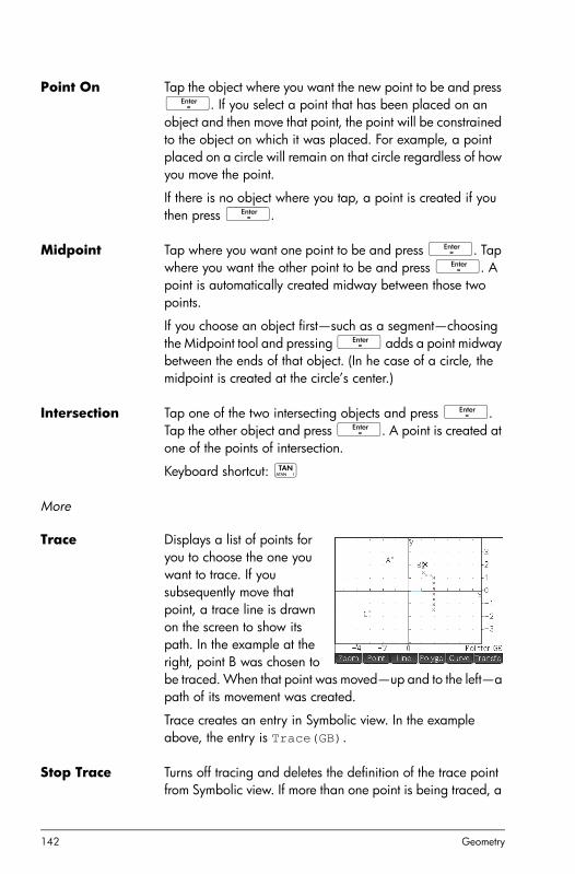
142 Geometry
Point On Tap the object where you want the new point to be and press E. If you select a point that has been placed on an object and then move that point, the point will be constrained to the object on which it was placed. For example, a point placed on a circle will remain on that circle regardless of how you move the point.
If there is no object where you tap, a point is created if you then press E.
Midpoint Tap where you want one point to be and press E. Tap where you want the other point to be and press E. A point is automatically created midway between those two points.
If you choose an object first—such as a segment—choosing the Midpoint tool and pressing E adds a point midway between the ends of that object. (In he case of a circle, the midpoint is created at the circle’s center.)
Intersection Tap one of the two intersecting objects and press E. Tap the other object and press E. A point is created at one of the points of intersection.
Keyboard shortcut: g
More
Trace Displays a list of points for you to choose the one you want to trace. If you subsequently move that point, a trace line is drawn on the screen to show its path. In the example at the right, point B was chosen to be traced. When that point was moved—up and to the left—a path of its movement was created.
Trace creates an entry in Symbolic view. In the example above, the entry is Trace(GB).
Stop Trace Turns off tracing and deletes the definition of the trace point from Symbolic view. If more than one point is being traced, a

Geometry 143
menu of trace points appears so that you can choose which one to untrace.
Untrace does not erase any existing trace lines. It merely prevents any further tracing should the point be moved again.
Erase Trace Erases all trace lines, but leaves the definition of the trace points in Symbolic view. While a Trace definition is still in Symbolic view, if you move the point again, a new trace line is created.
Center Tap a circle and press E.
Element 0 .. 1 ???????????
Intersections Tap one object and press E. Tap another object and press E. Each point of intersection is labeled (and labeled) identically. Note that an intersections object is created in Symbolic view even if the two objects selected do not intersect.
Random pts Displays a palette for you to choose to add 1, 2, 3, or 4 points. The points are placed randomly.
Line
Segment Tap where you want one endpoint to be and press E. Tap where you want the other endpoint to be and press E. A segment is drawn between the two end points.
Keyboard shortcut: r
Ray Tap where you want the endpoint to be and press E. Tap a point that you want the ray to pass through and press E. A ray is drawn from the first point and through the second point.
Line Tap at a point you want the line to pass through and press E. Tap at another point you want the line to pass through and press E. A line is drawn the two points.
Keyboard shortcut: j
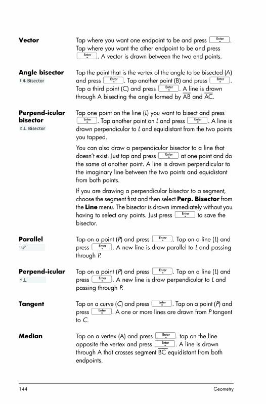
144 Geometry
Vector Tap where you want one endpoint to be and press E. Tap where you want the other endpoint to be and press E. A vector is drawn between the two end points.
Angle bisector Tap the point that is the vertex of the angle to be bisected (A) and press E. Tap another point (B) and press E. Tap a third point (C) and press E. A line is drawn through A bisecting the angle formed by AB and AC.
Perpend-icular bisector
Tap one point on the line (L) you want to bisect and press E. Tap another point on L and press E. A line is drawn perpendicular to L and equidistant from the two points you tapped.
You can also draw a perpendicular bisector to a line that doesn’t exist. Just tap and press E at one point and do the same at another point. A line is drawn perpendicular to the imaginary line between the two points and equidistant from both points.
If you are drawing a perpendicular bisector to a segment, choose the segment first and then select Perp. Bisector from the Line menu. The bisector is drawn immediately without you having to select any points. Just press E to save the bisector.
Parallel Tap on a point (P) and press E. Tap on a line (L) and press E. A new line is draw parallel to L and passing through P.
Perpend-icular Tap on a point (P) and press E. Tap on a line (L) and press E. A new line is draw perpendicular to L and passing through P.
Tangent Tap on a curve (C) and press E. Tap on a point (P) and press E. A one or more lines are drawn from P tangent to C.
Median Tap on a vertex (A) and press E. tap on the line opposite the vertex and press E. A line is drawn through A that crosses segment BC equidistant from both endpoints.

Geometry 145
Altitude Tap on a vertex (A) and press E. tap on the line opposite the vertex and press E. A line is drawn through A that crosses segment BC at right angles.
Polygon The Polygon menu provides tools for drawing various polygons.
Triangle Tap at each vertex, pressing E after each tap.
Keyboard shortcut: n
Quadilateral Tap at each vertex, pressing E after each tap.
Ngon
Polygon5 Produces a pentagon. Tap at each vertex, pressing E after each tap.
Polygon6 Produces a hexagon. Tap at each vertex, pressing E after each tap.
Hexagon Produces a regular hexagon (that is, one with sides of equal length). Tap at each vertex, pressing E after each tap.
Special
Eq. triangle Produces an equilateral triangle. Tap at one vertex and press E. Tap at another vertex and press E. The location of the third vertex is automatically calculated and the triangle is drawn.
Square Tap at one vertex and press E. Tap at another vertex and press E. Tap at a third vertex and press E. The location of the fourth vertex is automatically calculated and the square is drawn.
Parallel-ogram Tap at one vertex and press E. Tap at another vertex and press E. Tap at a third vertex and press E. The location of the fourth vertex is automatically calculated and the parallelogram is drawn.

146 Geometry
Curve
Circle Tap at the center of the circle and press E. Tap at point on the circumference and press E. A circle is drawn about the center point with a radius equal to the distance between the two tapped points.
Keyboard shortcut: F
You can also create a circle by first defining in Symbolic view. The syntax is circle(GA,GB) where A and B are two points. A circle is drawn in Plot view such that A and B are on the circumference.
Ellipse Tap at one focus point and press E. Tap at the second focus point and press E. Tap at point on the circumference and press E.
Hyperbola Tap at one focus point and press E. Tap at the second focus point and press E. Tap at point on one branch of the hyperbola and press E.
Parabola Tap at the focus point and press E. Tap either on a line (the directrix) or a point (the vertex) and press E.
Special
Circumcircle A circumcircle is the circle that passes through each of the triangle’s three vertices, thus enclosing the triangle.
Tap at each vertex of the triangle, pressing E after each tap.

Geometry 147
Incircle An incircle is a circle that is tangent to each of a polygon’s sides. The HP Prime can draw an incircle that is tangent to the sides of a triangle.
Tap at each vertex of the triangle, pressing E after each tap.
Excircle If you extend two sides of a triangle in the direction opposite their common vertex and then draw a circle tangent both to these lines and to the third side of the triangle, you have an excircle.
Tap at each vertex of the triangle, pressing E after each tap.
The excircle is drawn tangent to the side defined by the last two vertices tapped. In the example at the right, the last two vertices tapped were A and C (or C and A). Thus the excircle is drawn tangent to the segment AC.
Locus ???????????
Plot You can plot expressions of the following types in Plot view:
• Function
• Parametric
• Polar
• Sequence
• Slopefield

148 Geometry
Tap , select Plot, and then the type of expression you want to plot. The entry line is enabled for you to define the expression.
Note that the variables you specify for an expression must be in lowercase.
In this example, Function has been selected as the plot type and the graph of y = 1/x is plotted.
Geometric transformationsThe Transform menu—displayed by tapping
—provides numerous tools for you to transform a geometric object in Plot view.
Translation Translation is moving each point of an abject the same distance and in the sam direction. You create a vector to indicate the distance and direction of the translation, choose the object to be translated, and copy of the object to moved in line with the vector.
Suppose you want to move circle B at the right down a little and to the right:
1. Tap and select Vector.
2. Draw a vector in the direction you want to move the circle and of the same length as move you intend. (If you need help, see “Vector” on page 144.)
3. Tap .
4. Tap the vector and press E.

Geometry 149
5. Tap the object to be moved and press E.
The object is moved the same length as the vector and in the same direction. The original object is left in place.
Reflection Reflection is a transformation in which a copy of an object is made and every point on the new object is the same distance from a symmetry axis (or mirror line) as the original point. In the example at the right, the original triangle D is reflected an imaginary symmetry axis that passes through point I.
1. Tap and select Reflection.
2. Tap a point that will be in the symmetry axis (that is, mirror line) and press E.
3. Tap the object that is to be reflected across the symmetry axis and press E. The object is reflected across the symmetry axis defined by the point created at step 2.
Dilation Dilation is a transformation where an object is enlarged or reduced by a given factor around a given center point. The factor is sometimes referred to as the homothetic ratio (or scale factor) and the center point is called the homothetic center (or center of dilation).
the illustration at the right, the scale factor is 2 and the center of dilation is indicated by a point near the top right of the screen (named I). Each point on the new triangle is in line with its corresponding point on the original triangle and point I. Further, the distance from point I

150 Geometry
to each new point will be twice the distance to the original point (since the scale factor is 2).
1. Tap and select Dilation.
2. Tap the point that is to be the center of dilation and press E.
3. Enter the homothetic ratio (that is, the scale factor) and press E.
4. Tap the object that is to be dilated and press E.
Rotation Rotates a specified object about a specified point a specified number of degrees or radians.
[Not in Plot view, but available in Symbolic view. Broken as at May 18.]
More
Projection Creates an projection of the points on one object onto another object. The projection is orthogonal, that is, each projected point meets the object onto which it is projected at right angles.
1. Tap and select Projection.
2. Tap the object onto which points are to be projected and press E.
3. Tap the object that is to projected and press E.
Note the new points added to the target object.
Inversion Creates an inversion circle based on a specified center point, inversion ratio, and an inversion point on a line.
1. Tap and select Inversion.
2. Tap the point that is to be the center (C) of the inversion circle and press E.
Broken as at 18 May

Geometry 151
3. Enter the inversion ratio (r) and press E.
4. Tap on a line where you want the inversion point (B) to be and press E.
In the example at the right, the inversion ratio is 6 and the inversion point was a point tapped on line AB. Note that the center point and inversion point are not created as separate points.
Reciprocation To create a point that is the reciprocation of another point (or a line) with respect to a circle:
1. Tap and select Reciprocation.
2. Tap the circle and press E.
3. . Tap the point or line that is to generate the reciprocation point and press E.
In the example at the right, point H is the reciprocation of line G on circle C.
Geometry functions and commandsThe list of geometry-specific functions and commands in this section covers those that can be found by tapping in both Symbolic and Numeric view and those that are only available from the Catlg menu.
The sample syntax provided has been simplified. Geometric objects are referred to by a single uppercase character (such as A, B,C and so on). However, calculations referring to geometric objects—in the Numeric view of the Geometry app and in the CAS—must use the G-prefixed name given for it in Symbolic view. For example:
altitude(A,B,C) is the simplified form given in this section
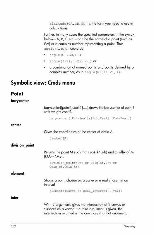
152 Geometry
altitude(GA,GB,GC) is the form you need to use in calculations
Further, in many cases the specified parameters in the syntax below—A, B, C etc.—can be the name of a point (such as GA) or a complex number representing a point. Thus angle(A,B,C) could be:
• angle(GP,GR,GB)
• angle(3+2i,1–2i,5+i) or
• a combination of named points and points defined by a complex number, as in angle(GP,i1–2i,i).
Symbolic view: Cmds menu
Pointbarycenter
barycenter([point1,coeff1],...) draws the barycenter of point1 with weight coeff1...
barycenter([Pnt,Real],[Pnt,Real],[Pnt,Real])
center
Gives the coordinates of the center of circle A.
center(A)
division_point
Returns the point M such that (z-a)=k*(z-b) and z=affix of M (MA=k*MB).
division_point(Pnt or Cplx(a),Pnt or Cplx(b),Cplx(k))
element
Shows a point chosen on a curve or a real chosen in an interval
element((Curve or Real_interval),[Val])
inter
With 2 arguments gives the intersection of 2 curves or surfaces as a vector. If a third argument is given, the intersection returned is the one closest to that argument.

Geometry 153
inter(Curve,Curve,[Pnt])
isobarycenter
isobarycenter(A,B,C,...) draws the isobarycenter of the n points A,B,C,...
midpoint
midpoint(A,B) draws the midpoint of the segment AB
midpoint((Pnt or Cplx),(Pnt or Cplx))
orthocenter
Shows the orthocenter of a triangle or of the triangle made with 3 points.
orthocenter((Pnt or Cplx),(Pnt or Cplx),(Pnt or Cplx))
point
A:=point(za) (resp A:=point([a,b,c])) draws a point of affix za (resp of coordinates (a,b,c)) with the legend A
point(Cplx(za)||Vect)
point2d
Defines at random, the coordinates (between -5 and +5) of the 2-d points given as argument.
point2d(SeqVar(A,B,C...))
trace
Turns on tracing of the specified point.
LineDrawSlp
Draws a line with slope m, going through the point (a, b).
DrawSlp(Real(a),Real(b),Real(m))
LineTan
Draws the tangent to y=f(x) at x=a.
LineTan(Expr(f(x)),[Var],Expr(a))

154 Geometry
altitude
Draws a line through A that crosses segment BC at right angles.
altitude(A,B,C)
bisector
Draws the bisector of the angle (AB,AC) given by 3 points A,B,C.
bisector((Pnt(A) or Cplx),(Pnt(B) or Cplx),(Pnt(C) or Cplx))
exbisector
Draws the exterior bisector of the angle (AB,AC) given by 3 points A,B,C.
exbisector((Pnt(A) or Cplx),(Pnt(B) or Cplx),(Pnt(C) or Cplx))
half_line
half_line(A,B) draws the half-line AB with A as origin
half_line((Pnt or Cplx),(Pnt or Cplx))
line
line(A,B) or line(a*x+b*y+c=0) or line(a*x+b*y+c*z+d=0,aa*x+bb*y+cc*z+dd=0) draws the line AB in the plane or in the 3D space. line(A,slope=m) draws the line going through A with slope m or of equation the argument in the plane or in 3D space.
line(Pnt||Cplx||Eq,[Pnt||slope||Var])
median_line
median_line(A,B,C) draws the median-line through A of the triangle ABC
median_line((Pnt or Cplx),(Pnt or Cplx),(Pnt or Cplx))
parallel
parallel(A,D) (resp parallel(A,P) or parallel(A,D,DD)) draws the line (resp plane) through A parallel to the line D (resp parallel to the plane P or to the lines D,DD) and, parallel(d,D) draws the plane through d parallel to the line D.
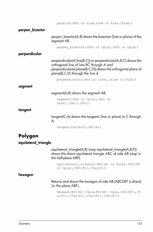
Geometry 155
parallel(Pnt or Line,Line or Plan,[Line])
perpen_bisector
perpen_bisector(A,B) draws the bisection (line or plane) of the segment AB.
perpen_bisector((Pnt or Cplx),(Pnt or Cplx))
perpendicular
perpendicular(A,line(B,C)) or perpendicular(A,B,C) draws the orthogonal line of line BC through A and perpendicular(d,plane(B,C,D)) draws the orthogonal plane of plane(B,C,D) through the line d.
perpendicular((Pnt or Line),(Line or Plan))
segment
segment(A,B) draws the segment AB
segment((Pnt or Cplx),(Pnt or Cplx),[Var],[Var])
tangent
tangent(C,A) draws the tangents (line or plane) to C through A.
tangent(Curve(C),Pnt(A))
Polygonequilateral_triangle
equilateral_triangle(A,B) (resp equilateral_triangle(A,B,P)) draws the direct equilateral triangle ABC of side AB (resp in the half-plane ABP).
equilateral_triangle((Pnt(A) or Cplx),(Pnt(B) or Cplx),[Pnt(P)],[Var(C)])
hexagon
Returns and draws the hexagon of side AB (ABCDEF is direct) (in the plane ABP.)
hexagon(Pnt(A)||Cplx,Pnt(B)||Cplx,[Pnt(P)],[Var(C)],[Var(D)],[Var(E)],[Var(F)])

156 Geometry
isosceles_triangle
Draws the isosceles triangle ABC AB=AC and angle(AB,AC)=t (or in the plane ABP angle(AB,AC)=angle(AB,AP) or angle(AB,AC)=t).
isosceles_triangle((Pnt(A) or Cplx),(Pnt(B) or Cplx),(Angle(t) or Pnt(P) or Lst(P,t)),[Var(C)] )
isopolygon
Draws a regular polygon having abs(n) vertices, given by 2 vertices (or 2 vertices and 1 point of the plane) if n>0 and by its center and 1 vertex (or its center, 1 vertex and 1 point of the plane) if n<0.
isopolygon(Pnt,Pnt,[Pnt],Intg(n))
parallelogram
Returns and draws the parallelogram ABCD such as vector(AB)+vector(AD)=vector(AC).
parallelogram(Pnt(A)||Cplx,Pnt(B)||Cplx,Pnt(C)||Cplx,[Var(D)] )
polygon
Returns and draws the polygon where its vertices are the element of l.
polygon(LstPnt||LstCplx)
quadrilateral
Returns and draws the quadrilateral ABCD.
quadrilateral(Pnt(A)||Cplx,Pnt(B)||Cplx,Pnt(C)||Cplx,Pnt(D)||Cplx)
rectangle
Returns and draws the rectangle ABCD, AD=k*AB if k>0 ABCD is direct else indirect (in the plane ABP AD=AP or AD=k*AB).
rectangle(Pnt(A)||Cplx,Pnt(B)||Cplx,Real(k)||Pnt(P)||Lst(P,k),[Var(D)],[Var(C)])

Geometry 157
rhombus
Returns and draws the rhombus ABCD such as the angle (AB,AD)=a (or in the plane ABP angle(AB,AD)=angle(AB,AP) or such that angle(AB,AD)=a).
rhombus(Pnt(A)||Cplx,Pnt(B)||Cplx,Angle(a)||Pnt(P)||Lst(P,a)),[Var(C)],[Var(D)])
right_triangle
Draws the A_rectangular triangle ABC with AC=k*AB (or in the plane ABP AC=AP or AC=k*AB).
right_triangle((Pnt(A) or Cplx),(Pnt(B) or Cplx),(Real(k) or Pnt(P) or Lst(P,k)),[Var(C)])
square
Returns and draws the square of side AB (ABCD is direct) (in the plane ABP.
square((Pnt(A) or Cplx),(Pnt(B) or Cplx),[Pnt(P),Var(C),Var(D)])
triangle
triangle(A,B,C) draws the triangle ABC
triangle((Pnt or Cplx),(Pnt or Cplx),(Pnt or Cplx))
CurveFunction
Defines a function plot.
plotfunc(Expr)
circle
Define for 2-d a circle with a diameter (arg2=Point) or with center and radius (arg2=Complex, abs(arg2)=radius)
[or the arc AB, A angle a, B angle b (arg1+arg2=angle 0)] or by its equation and for 3-d with a diameter and a third point
circle((Pnt or Cplx),(Pnt(arg2) or Cplx(arg2)),[Real(a)],[Real(b)],[Var(A)],[Var(B)])

158 Geometry
circumcircle
circumcircle(A,B,C)=circumcircle of the triangle ABC.
circumcircle((Pnt or Cplx),(Pnt or Cplx),((Pnt or Cplx))
conic
Defines a conic by its equation with x,y as default variables and draws it.
conic(Expr,[LstVar])
ellipse
ellipse(F1,F2,M)=ellipse focus F1,F2 through M or such as MF1+MF2=2*a (geo2d) and ellipse(p(x,y)) draws the conic if deg(p)=2.
ellipse(Pnt(F1),Pnt(F2),(Pnt(M) or Real(a)) y ellipse(p(x,y))=conic si deg(p)=2.)
excircle
excircle(A,B,C) draws the A-excircle of the ABC triangle.
excircle((Pnt or Cplx),(Pnt or Cplx),(Pnt or Cplx))
hyperbola
hyperbola(F1,F2,M)=hyperbola focus F1,F2 through M or (|MF1-MF2|=2*a geo2d) and hyperbola(p(x,y)) draws the conic if deg(p)=2.
hyperbola(Focus(F1),Focus(F2),(Pnt(M) or Real(a)))
incircle
incircle(A,B,C) draws the incircle of the ABC triangle.
incircle((Pnt or Cplx),(Pnt or Cplx),(Pnt or Cplx))
locus
locus(M,A) draws the locus of M (or locus(d,A) draws the envelope of d) when A:=element(C) (C is a curve). The example instructions below must be written in a geometric level on different lines.
locus(Pnt,Elem)
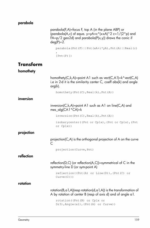
Geometry 159
parabola
parabola(F,A)=focus F, top A (in the plane ABP) or (parabola(A,c) of equa. y=yA+c*(x-xA)^2 c=1/(2*p) and FA=p/2 geo2d) and parabola(P(x,y)) draws the conic if deg(P)=2.
parabola(Pnt(F)||Pnt(xA+i*yA),Pnt(A)||Real(c),[Pnt(P)])
Transformhomothety
homothety(C,k,A)=point A1 such as vect(C,A1)=k*vect(C,A) i.e in 2-d it is the similarity center C, coeff abs(k) and angle arg(k).
homothety(Pnt(C),Real(k),Pnt(A))
inversion
inversion(C,k,A)=point A1 such as A1 on line(C,A) and mes_alg(CA1*CA)=k
inversion(Pnt(C),Real(k),Pnt(A))
isobarycenter((Pnt or Cplx),(Pnt or Cplx),(Pnt or Cplx))
projection
projection(C,A) is the orthogonal projection of A on the curve C
projection(Curve,Pnt)
reflection
reflection(D,C) (or reflection(A,C))=symmetrical of C in the symmetry-line D (or sym-point A)
reflection((Pnt(A) or Line(D)),(Pnt(C) or Curve(C)))
rotation
rotation(B,a1,A)(resp rotation(d,a1,A)) is the transformation of A by rotation of center B (resp of axis d) and of angle a1.
rotation((Pnt(B) or Cplx or Dr3),Angle(a1),(Pnt(A) or Curve))
160 Geometry
similarity
similarity(B,k,a1,A)=transformation of A in the similarity (center B or axis d, coeff k,angle a1) (or also homothety(B,k*exp(i*a1),A)).
similarity(Pnt or Dr3,Real,Angle,Pnt)
translation
translation(B-A,C) (resp translation([a,b,c],C)) is the translation of C in the translation of vector AB (resp [a,b,c]).
translation(Vect, Pnt(C))
Numeric view: Cmds menu
Measureabscissa
The x coordinate of a point or the x length of a vector.
abscissa(A) or abscissa(vector)
affix
Gives the affix of a point (that is, its coordinates expressed as a complex number) or the affix of a vector.
affix(A) or affix(vector)
angle
Calculates the angle made by AB and AC.
angle(A,B,C)
arcLen
Returns the length of the arc of the curve defined by y=Xpr (or by x=Xpr1,y=Xpr2) when the parameter values are between a and b.
arcLen(Expr(Xpr) or Lst([Xpr1,Xpr2]),Var,Real(a),Real(b))
area
Algebraic area of a circle or polygon or of the area below a curve, optionally with a quadrature method (trapezoid, left_rectangle, right_rectangle, middle_point, simpson, rombergt, rombergm).

Geometry 161
area(Polygon) or area(Expr,x=a..b,[n],[Method])
coordinates
Returns the list (resp matrix) of the abscissa and of the ordinate of a point or a vector (resp of points or vectors).
coordinates(Pnt or Cplx or Vect)
distance
Calculates the distance between 2 points or a point and a curve
distance((Pnt or Cplx),(Pnt or Cplx or Curve))
distance2
Calculates the square of the distance between 2 points or a point and a curve
distance2((Pnt or Cplx),(Pnt or Cplx or Curve))
distanceat
distanceat(A,B,z0) displays at point(z0), with a legend, the distance between 2 geometrical objects
distanceat(GeoObj(A),GeoObj(B),(Pnt or Cplx))
distanceatraw
distanceatraw(A,B,z0) displays at the point(z0), the distance between 2 geometrical objects.
distanceatraw(GeoObj(A),GeoObj(B),(Pnt or Cplx(z0)))
equation
equation returns the cartesian equation of a curve
equation(GeoObj, VectParam)
extract_measure
extract_measure gives as answer the value calculated by the argument.
extract_measure(Var)
ordinate
Returns the ordinate of a point or a vector.

162 Geometry
ordinate(Pnt or Vect)
parameq
parameq(C) returns the complex number=parametric equation of the curve C
parameq(GeoObj )
perimeter
Perimeter of a polygon (e.g. triangle, square, ...)
perimeter(Polygon)
radius
radius(C) gives the radius of the circle C
radius(Crcle)
Testis_collinear
Returns 1 if the points are aligned,2 if the points are the same and 0 otherwise.
is_collinear(LstPnt)
is_concyclic
Returns 1 if the points are on a circle and 0 otherwise.
is_concyclic(LstPnt)
is_conjugate
Returns 1 if the 3 (resp 4) arguments are conjugated toward a circle (resp 2 lines) and 0 otherwise.
is_conjugate(Crcle||Line,Pnt||Line,Pnt||Line,[Pnt||Line])
is_coplanar
Test if 4 points are in the same plane.
is_coplanar(Pnt,Pnt,Pnt,Pnt)
is_element
Returns 1 if the point is on the geometric object and 0 otherwise.
is_element(Pnt,GeoObj)

Geometry 163
is_equilateral
Returns 1 if the 3 points (or the object) build an equilateral triangle and 0 otherwise.
is_equilateral(Pnt||Cplx,Pnt||Cplx,Pnt||Cplx)
is_isoceles
Returns 1, 2 or 3 if the 3 points (or the object) build an isosceles triangle with vertices 1, 2, or 3, returns 4 if the 3 points (or the object) build an equilateral triangle and 0 otherwise.
is_isosceles(Pnt or Cplx,Pnt or Cplx,Pnt or Cplx)
is_orthogonal
Returns 1 if the 2 circles are orthogonal (orthogonal tangents at a point of intersection) or if the 2 lines are orthogonal and 0 otherwise.
is_orthogonal(Line||Crcle,Line||Crcle)
is_parallel
Returns 1 if 2 lines are parallel and 0 otherwise.
is_parallel(Line or Plan ,Line or Plan)
is_parallelogram
Returns 1, 2, 3 or 4 if the 4 points (or the object) build a parallelogram, (2 for a rhombus, 3 for a rectangle, 4 for a square) and 0 otherwise.
is_parallelogram(Pnt or Cplx,Pnt or Cplx,Pnt or Cplx,Pnt or Cplx)
is_perpendicular
Returns 1 if 2 lines are perpendicular
is_perpendicular(Line or Plan,Line or Plan)
is_rectangle
Returns 1, 2 or 3 if the 3 points (or the object) build a rectangular triangle with vertex 1, 2 or 3 and 0 otherwise [or 1 if the 4 points (or the object) build a rectangle, 2 if the 4 points (or the object) build a square and 0 otherwise].
is_rectangle(Pnt||Cplx,Pnt||Cplx,Pnt||Cplx,[Pnt||Cplx])

164 Geometry
is_square
Returns 1 if the 4 points build a square and 0 otherwise.
is_square(Pnt,Pnt,Pnt,Pnt)
Other Geometry functionsThe following functions are not available from a menu in the Geometry app, but are available from the Catlg menu.
angleat
angleat(A,B,C,z0) displays at point(z0) the value of the measure of the angle made by AB and AC along with a legend.
angleat(A,B,C,z0)
angleatraw
Same as angleat but without providing a legend.
areaat
Displays at point (z0), with a legend, algebraic area of a circle or of a (star) polygon (e.g. triangle, square, ...)
areaat(Polygon, Pnt||Cplx(z0))
areaatraw
Displays at point(z0), algebraic area of a circle or of a (star) polygon (e.g. triangle, square, ...)
areaatraw(Polygone, Pnt||Cplx(z0))
common_perpendicular
Draws the common perpendicular of the lines D1 and D2.
common_perpendicular(Line(D1),Line(D2))
cone
Draws a cone with vertex A, direction v, and with half-angle t [and with altitude h and -h].
cone(Pnt(A),Vect(v),Real(t),[Real(h)])
convexhull
Convex hull of a list of 2-d points

Geometry 165
convexhull(Lst)
cube
Draws the direct cube with vertices A,B with a face in the plan (A,B,C).
cube(Pnt(A),Pnt(B),Pnt(C))
cylinder
Draws a cylinder with axis (A,v), with radius r [and with altitude h].
cylinder(Pnt(A),Vect(v),Real(r),[Real(h)])
display
Draws an geometrical object with color (black=0 red=1 green=2 yellow=3 blue=4). If object is closed, object can be filled. Line_width_n (0<n<8) is for the width of the line and dash_line is for dotted line.
display(circle(0,1),2) returns a green circle of radius 1.
display(square(0,5),filled+blue+line_width_6) returns a blue square of sides 5, filled with blue and a of line width of 6.
faces
Returns the list of the faces (1 face=matrix(n,3) where the n rows are the n vertices of the face) of the polyhedron P.
faces(Polygon or Polyedr(P))
half_cone
Draws a half-cone with vertex A, direction v and with half_angle=t [and with altitude h].
half_cone(Pnt(A),Vect(v),Real(t),[Real(h)])
harmonic_conjugate
Returns the harmonic conjugate of 3 points or of 3 parallel or concurrent lines or the line of conjugates of a point in respect to 2 lines.
harmonic_conjugate(Line or Pnt,Line or Pnt,Line or Pnt)
166 Geometry
harmonic_division
Returns the 4 points (resp lines) and affects the last argument, such as the 4 points (resp lines) are in a harmonic division.
harmonic_division(Pnt or Line,Pnt or Line,Pnt or Line,Var)
icosahedron
Draws an icosahedron with center A, vertex B and such that the plane ABC contains one vertex among the 5 nearest vertices from B.
icosahedron(Pnt(A),Pnt(B),Pnt(C))
is_harmonic
Returns 1 if the 4 points are in a harmonic division and 0 otherwise.
is_harmonic(Pnt or Cplx,Pnt or Cplx,Pnt or Cplx,Pnt or Cplx)
is_harmonic_circle_bundle
Returns 1 if the circles build a beam, 2 if they have the same center, 3 if they are the same and 0 otherwise.
is_harmonic_circle_bundle(Lst(Crcle))
is_harmonic_line_bundle
Returns 1 if the lines have a common point, 2 if they are parallels, 3 if they are the same and 0 otherwise.
is_harmonic_line_bundle(Lst(Line))
is_rhombus
Returns 1 or 2 if the 4 points (or the object) build a rhombus (2 for a square) and 0 otherwise.
is_rhombus(Pnt or Cplx,Pnt or Cplx,Pnt or Cplx,Pnt or Cplx)
length
Returns the size of a list, a string or a sequence
length(Lst or Str or Seq)
LineHorz
Draws the horizontal line y=a.
Geometry 167
LineHorz(A)
line_segments
Returns the list of the line_segments (1 line=segment) of the polyhedron P
line_segments(Polygon or Polyedr(P))
LineVert
Draws the vertical line x=a.
LineVert(Expr(a))
octahedron
Draws an octahedron with center A, vertex B and such that the plane ABC contains 4 vertices.
octahedron(Pnt(A),Pnt(B),Pnt(C))
open_polygon
Returns and draws the polygonal line where its vertices are the element of l.
open_polygon(LstPnt||LstCplx)
orthogonal
orthogonal(A,line(B,C)) draws the orthogonal plane of line BC through A and orthogonal(A,plane(B,C,D)) draws the orthogonal line of plan(B,C,D) through A.
orthogonal((Pnt),(Line or Plan) )
parallelepiped
Draws a parallelepiped with sides AB,AC,AD (the faces are parallelograms).
parallelepiped(Pnt(A),Pnt(B),Pnt(C),Pnt(D))
perimeterat
Displays at point(z0), with a legend, the perimeter of a circle or of a polygon (e.g. triangle, square, ...)
perimeterat(Polygon, Pnt||Cplx(z0))
perimeteratraw
Displays at point(z0), the perimeter of a circle or of a polygon (e.g. triangle, square, ...)
168 Geometry
perimeteratraw(Polygon, Pnt||Cplx(z0))
plane
plane(A,B,C) or plane(A,line(B,C)) (resp plane(a*x+b*y+c*z+d=0)) draws the plane ABC (resp of equation a*x+b*y+c*z+d=0) in the 3-D space.
plane(Pnt or Eq, [Pnt or Line],[Pnt])
polar
Returns the line of the conjugated points of A with respect to the circle.
polar(Crcle,Pnt or Cplxe(A))
polar_coordinates
Returns the list of the norm and of the argument of the affix of a point (for 2-D) or of a complex number or of the the list of rectangular coordinates.
polar_coordinates(Pnt or Cplx or LstRectCoord)
pole
Returns the point having the line as polar with respect to the circle.
pole(Crcle,Line)
polyhedron
Draws a convex polyhedron with vertices among the arguments.
polyhedron(SeqPnt(A,B,C...))
powerpc
Returns the real number d^2-R^2 (d=distance between point and center, R=radius) .
powerpc(Circle,Pnt or Cplx)
prism
Draws a prism with plane base ABCD...and with edges parallel to AA1 (the faces are parallelograms).
prism(LstPnt([A,B,C,D]),Pnt(A1))
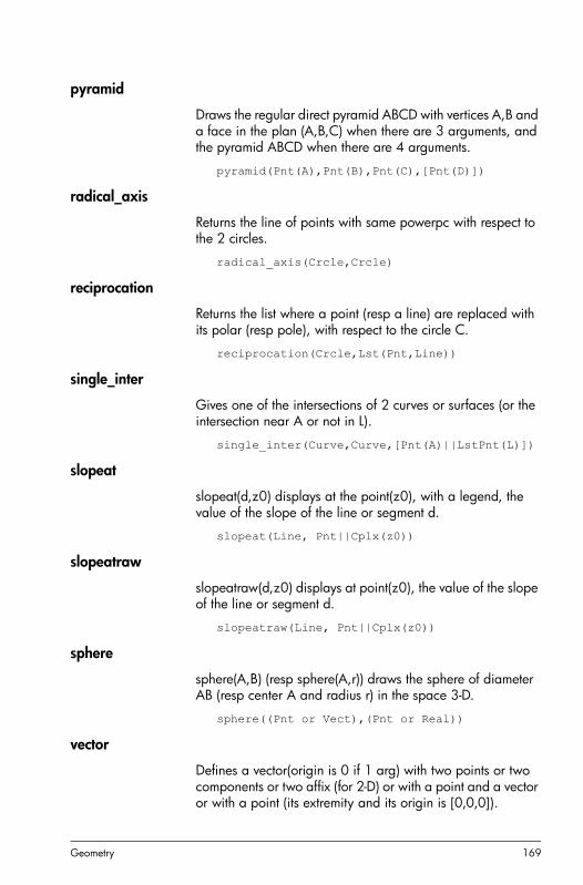
Geometry 169
pyramid
Draws the regular direct pyramid ABCD with vertices A,B and a face in the plan (A,B,C) when there are 3 arguments, and the pyramid ABCD when there are 4 arguments.
pyramid(Pnt(A),Pnt(B),Pnt(C),[Pnt(D)])
radical_axis
Returns the line of points with same powerpc with respect to the 2 circles.
radical_axis(Crcle,Crcle)
reciprocation
Returns the list where a point (resp a line) are replaced with its polar (resp pole), with respect to the circle C.
reciprocation(Crcle,Lst(Pnt,Line))
single_inter
Gives one of the intersections of 2 curves or surfaces (or the intersection near A or not in L).
single_inter(Curve,Curve,[Pnt(A)||LstPnt(L)])
slopeat
slopeat(d,z0) displays at the point(z0), with a legend, the value of the slope of the line or segment d.
slopeat(Line, Pnt||Cplx(z0))
slopeatraw
slopeatraw(d,z0) displays at point(z0), the value of the slope of the line or segment d.
slopeatraw(Line, Pnt||Cplx(z0))
sphere
sphere(A,B) (resp sphere(A,r)) draws the sphere of diameter AB (resp center A and radius r) in the space 3-D.
sphere((Pnt or Vect),(Pnt or Real))
vector
Defines a vector(origin is 0 if 1 arg) with two points or two components or two affix (for 2-D) or with a point and a vector or with a point (its extremity and its origin is [0,0,0]).

170 Geometry
vector(Pnt,Pnt || Pnt,Vect)
vertices
Returns the list of the vertices of the polygon or polyhedron P.
vertices(Polygon or Polyedr(P))
vertices_abca
Returns the closed list [A,B,...A] of the vertices of the polygon or polyhedron P.
vertices_abca(Polygon or Polyedr(P)

Spreadsheet 171
8
Spreadsheet
The Spreadsheet app provides a grid of cells for you to enter content (such as numbers, text, expressions, and so on) and to perform certain operations on what you enter.
To open the Spreadsheet app, press I and select Spreadsheet.
You can create any number of customized spreadsheets, each with its own name (see “Creating an app” on page 97). You open a customized spreadsheet in the same way: by pressing I and selecting the particular spreadsheet.
The maximum size of any one spreadsheet is 10,000 rows by 676 columns.
The app opens in Numeric view. There is no Plot or Symbolic view. There is a Symbolic Setup view (SY) that enables you to override certain system-wide settings. (See “Common operations in Symbolic Setup view” on page 76.)
Getting started with the Spreadsheet appSuppose you have a stall at a weekend market. You sell furniture on consignment for their owners, taking a 10% commission for yourself. You have to pay the landowner $100 a day to set up your stall and you will keep the stall open until you have made $250 for yourself.
1. Open the Spreadsheet app:
I and select Spreadsheet.
2. Select column A. Either tap on A or use the cursor keys to highlight the A cell (that is, the heading of the A column).

172 Spreadsheet
3. Enter PRICE and tap . You have named the entire first column PRICE.
4. Select column B. Either tap on B or use the cursor keys to highlight the B cell.
5. Enter a formula for your commission (being 10% of the price of each item sold):
S.PRICEs0.1E
Because you entered the formula in the heading of a column, it is automatically copied to every cell in that column. At the moment only 0 is shown, since there are no values in the PRICE column yet.
6. Once again select the header of column B.
7. Tap and select Name.
8. Type COMMIS and tap .
Note that the heading of column B is now COMMIS.
9. It is always a good idea to check your formulas by entering some dummy values and noting if the result is as expected. Select cell A1 and make sure that and not is showing in the menu. (If not, tap the button.) This option means that your cursor automatically selects the cell immediately below the one you have just entered content into.
10.Add some values in the PRICE column and note the result in the COMMIS column. If the results do not look right, you can tap the COMMIS heading, tap
and fix the formula.

Spreadsheet 173
11. To delete the dummy values, select cell A1, tap , press \ until all the dummy values are selected, and then press C.
12. Select cell C1.
13. Enter a label for your takings:
S.ANTAKINGSE
Notice that text strings, but not names, need to be enclosed within quotation marks.
14. Select cell D1.
15. Enter a formula to add up your takings:
S.SUM R PRICE E
You could have specified a range—such as A1:A100—but by specifying the name of the column, you can be sure that the sum will include all the entries in the column.
16. Select cell C3.
17. Enter a label for your total commission:
S.ANTOTAL COMMISE
Note that the column is not wide enough for you to see the entire label in C3. We need to widen column C.
18. Select the heading cell for column C, tap and select Column .
An input form appears for you to specify the required width of the column.
19. Enter 100 and tap .
You may have to experiment until you get the column width exactly as you want it. The value you enter will be the width of the column in pixels.
20.Select cell D3.
21. Enter a formula to add up your commission:
S.SUM R COMMIS E
Note that instead of entering SUM by hand, you could have chosen it from the Apps menu (one of the Toolbox menus).
22.Select cell C5.
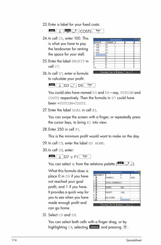
174 Spreadsheet
23.Enter a label for your fixed costs:
S.ANCOSTSE
24.In cell C5, enter 100. This is what you have to pay the landowner for renting the space for your stall.
25.Enter the label PROFIT in cell C7.
26. In cell D7, enter a formula to calculate your profit:
S.D3 w D5E
You could also have named D3 and D5—say, TOTCOM and COSTS respectively. Then the formula in D7 could have been =TOTCOM–COSTS.
27. Enter the label GOAL in cell E1.
You can swipe the screen with a finger, or repeatedly press the cursor keys, to bring E1 into view.
28.Enter 250 in cell F1.
This is the minimum profit would want to make on the day.
29. In cell C9, enter the label GO HOME.
30.In cell D9, enter:
S.D7 ≥ F1E
You can select ≥ from the relations palette (Sv).
What this formula does is place 0 in D9 if you have not reached your goal profit, and 1 if you have. It provides a quick way for you to see when you have made enough profit and can go home.
31. Select C9 and D9.
You can select both cells with a finger drag, or by highlighting C9, selecting and pressing >.

Spreadsheet 175
32. Tap and select Color.
33.Choose a color for the contents of the selected cells.
34.Tap and select Fill.
35.Choose a color for the background of the selected cells.
The most important cells in the spreadsheet will now stand out from the rest.
The spreadsheet is complete, but you may want to check all the formulas by adding some dummy data to the PRICE column. When the profit reaches 250, you should see the value in D9 change from 0 to 1.
Basic operations
Navigation, selection and gesturesYou can move about a spreadsheet by using the cursor keys, by swiping, or by tapping and specifying the cell you want to move to.
You select a cell simply by moving to it. You can also select an entire column—by tapping the column letter—and select an entire row (by tapping the row number). You can also select the entire spreadsheet: just tap on the unnumbered cell at the top-left corner of the spreadsheet. (It has the HP logo in it.)
A block of cells can be selected by pressing down on a cell that will be a corner cell of the selection and, after a second, dragging your finger to the diagonally opposite cell. You can also select a block of cells by moving to a corner cell, tapping
and using the cursor keys to move to the diagonally opposite cell. Tapping on or another cell deselects the selection.

176 Spreadsheet
Cell referencesYou can refer to the value of a cell in formulas as if it were a variable. A cell is referenced by its column and row coordinates, and references can be absolute or relative. An absolute reference is written as $C$R (where C is the column number and R the row number). Thus $B$7 is an absolute reference. In a formula it will always refer to the data in cell B7 wherever that formula, or a copy of it, is placed. On the other hand, B7 is a relative reference. It is based on the relative position of cells. Thus a formula in, say, B8 that references B7 will reference C7 instead of B7 if it is copied to C8.
Ranges of cells can also be specified, as in C6:E12, as can entire columns (E:E) or entire rows ($3:$5). Note that the alphabetic component of column names can be uppercase or lowercase except for columns g, l, m, and z. These must be in lowercase if not preceded by $. Thus cell B1 can be referred to as B1,b1,$B$1 or $b$1 whereas M1 can only be referred to as m1, $m$1, or $M$1. (G, L, M, and Z are names reserved for graphic objects, lists, matrices, and complex numbers.)
Cell namingCells, blocks of cells, rows, and columns can be named. The name can then be used in a formula. A named cell or block of cells is given a blue border.
Method 1 To name an empty cell, row, or column, go the cell, row header, or column header, enter a name and tap .
Method 2 To name a cell, block, row, or column—whether it is empty or not:
1. Select the cell, block, row, or column.
2. Tap and select Name.
3. Enter a name and tap .
Using names in calculations
The name you give a cell or block of cells can be used in a formula. For example, if you name a cell TOTAL, you could enter in another cell the formula =TOTAL*1.1.

Spreadsheet 177
The following is a more complex example involving the naming of an entire column.
1. Select cell A (that is the header cell for column A).
2. Enter COST and tap .
3. Select cell B (that is the header cell for column B).
4. Enter S.COST*0.33 and tap .
5. Enter some values in column A and observe the calculated results in column B.
Entering contentYou can enter content directly in the spreadsheet or import data from a statistics app.
Direct entry A cell can contain any valid calculator object: a real number (3.14), a complex number (a + ib), an integer (#1Ah), a list ({1, 2}), a matrix or vector([1, 2]), a string ("text"), a unit (2_m) or an expression (that is, a formula). Move to the cell you want to add content to and start entering the content as you would in Home view. Press E when you have finished. You can also enter content into a number of cells with a single entry. Just select the cells, enter the content—for example, =Row*3—and press E.
What you enter on the entry line is evaluated as soon as you press E, with the result placed in the cell or cells. However, if you want to retain the underlying formula, precede it with S.. For example, suppose that want to add cell A1 (which contains 7) to cell B2 (which contains 12). Entering A1+ B2E in, say, A4 yields19, as does entering S.A1+ B2 in A5. However, if the value in A1 (or B2) changes, the value in A5 changes but not the value in A4. This is because the expression (or formula) was retained in A5. To see if a cell contains just the value shown in it or also an

178 Spreadsheet
underlying formula that generates the value, move your cursor to the cell. The entry line shows a formula if there is one.
A single formula can add content to every cell in a column or row. For example, move to C (the heading cell for column C), enter S.SIN(Row)and press E. Each cell in the column is populated with the sine of the cell’s row number. A similar process enables you to populate every cell in a row with the same formula. You can also add a formula once and have it apply to every cell in the spreadsheet. You do this by placing the formula in the cell at the top left (the cell with the HP logo in it). To see how this works, suppose you want to generate a table of powers (squares, cubes, and so on) starting with the squares:
1. Tap on the cell with the HP logo in it (at the top left corner). Alternatively, you can use the cursor keys to move to that cell (just as you can to select a column or row heading).
2. On the entry line type S.RowkRCol+1
Note that Row and Col are built-in variables. They are placeholders for the row number and column number of the cell that has a formula containing them.
3. Tap or Press E.
Note that each column gives the nth power of the row number starting with the squares. Thus 95 is 59,049.
Import data You can import data from the Statistics 1Var and Statistics 2Var apps (and from any app customized from a statistics app). In the procedure immediately below, dataset D1 from the Statistics 1Var app is being imported.
1. Select a cell.
2. Enter Statistics_1Var.D1.
3. Press E.

Spreadsheet 179
The column is filled with the data from the statistics app, starting with the cell selected at step 1. Any data in that data will be overwritten by the data being imported.
You can also export data from the Spreadsheet app to a statistics app. See “Entering and editing statistical data” on page 191 for the general procedure. It can be used in both the Statistics 1Var and Statistics 2Var apps.
External functions
You can use in a formula any function available on the Math, CAS, App, User or Catlg menus (see chapter 20, “Functions and commands” on page 283). For example, to find the root of 3 – x2 closest to x = 2, you could enter in a cell S.AAROOTAR3wAsjo2E. The answer displayed is 1.732…
You could also have selected a function from a menu. For example:
1. Press S..
2. Press D and tap .
3. Select Polynomial > Find Roots.
Your entry line will now look like this: =CAS.proot().
4. Enter the coefficients of the polynomial, in descending order, separating each with a comma:
Q1 o0o3
5. Press E to see the result: 1.732…
Note that the CAS prefix added to your function is to remind you that the calculation will be carried out by the CAS (and thus a symbolic result will be returned, if possible). You can also force a calculation to be handled by the CAS by tapping in the spreadsheet.
There are additional spreadsheet functions that you can use (mostly related to finance and statistics calculations). See “Spreadsheet functions” on page 314.

180 Spreadsheet
Copy and pasteTo copy one or more cells, select them and press SV (Copy).
Move to the desired location and press (SZ (Paste).
You can choose to paste either the value, formula, format, both value and format, or both formula and format.
External referencesYou can refer to data in a spreadsheet from outside the Spreadsheet app by using the reference SpreadsheetName.CR. For example, in Home view you can refer to cell A6 in the built-in spreadsheet by entering Spreadsheet.A6. Thus the formula 6*Spreadsheet.A6 would multiply whatever value is currently in cell A6 in the built-in app by 6.
If you have created a customized spreadsheet called, say, Savings, you simply refer to it by its name, as in 5*Savings.A6.
An external reference can also be to a named cell, as in 5*Savings.TOTAL.
In the same way, you can also enter references to spreadsheet cells in the CAS.
If you are working outside a spreadsheet, you cannot refer to a cell by its absolute reference. Thus Spreadsheet.$A$6 produces an error message.
Note that a reference to a spreadsheet name is case-sensitive.

Spreadsheet 181
Referencing variablesAny variable can be inserted in a spreadsheet cell. This includes Home variables, App variables, CAS variables and user variables.
Variables can be referenced or entered. For example, if you have assigned 10 to P in Home view, you could enter =P*5 in a spreadsheet cell, press E and get 50. If you subsequently changed the value of P, the value in that cell automatically changes to reflect the new value. This is an example of a referenced variable.
If you just wanted the current value of P and not have the value change if P changed, just enter P and press E. This is an example of an entered variable.
Variables given values in other apps can also be referenced in a spreadsheet. In chapter 12 we see how the Solve app can be used to solve equations. An example used is V 2 = U 2 + 2AD. You could have four cells in a spreadsheet with =V, =U, =A, and =D as formulas. As you experiment with different values for these variables in the Solve app, the entered and the calculated values are copied to the spreadsheet (where further manipulation could be done).
The variables from other apps includes the results of certain calculations. For example, if you have plotted a function in the Function app and calculated the signed area between two x-values, you can reference that value in a spreadsheet by pressing a, tapping , and then selecting Function > Results > SignedArea.
Numerous system variables are also available. For example, you could enter S+E to get the last answer calculated in Home view. You could also enter S.S+E to get the last answer calculated in Home view and have the value automatically updated as new calculations are made in Home view. (Note that this works only with the Ans from Home view, not the Ans from CAS view.)
All the variables available to you are listed on the variables menus, displayed by pressing a. A comprehensive list of

182 Spreadsheet
these variables is provided in chapter 21, “Variables”, beginning on page 373.
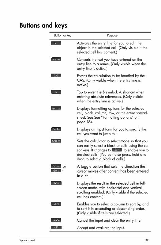
Spreadsheet 183
Buttons and keysButton or key Purpose
Activates the entry line for you to edit the object in the selected cell. (Only visible if the selected cell has content.)
Converts the text you have entered on the entry line to a name. (Only visible when the entry line is active.)
Forces the calculation to be handled by the CAS. (Only visible when the entry line is active.)
Tap to enter the $ symbol. A shortcut when entering absolute references. (Only visible when the entry line is active.)
Displays formatting options for the selected cell, block, column, row, or the entire spread-sheet. See See “Formatting options” on page 184.
Displays an input form for you to specify the cell you want to jump to.
Sets the calculator to select mode so that you can easily select a block of cells using the cur-sor keys. It changes to to enable you to deselect cells. (You can also press, hold and drag to select a block of cells.)
or :
A toggle button that sets the direction the cursor moves after content has been entered in a cell.
Displays the result in the selected cell in full-screen mode, with horizontal and vertical scrolling enabled. (Only visible if the selected cell has content.)
Enables you to select a column to sort by, and to sort it in ascending or descending order. (Only visible if cells are selected.)
Cancel the input and clear the entry line.
Accept and evaluate the input.

184 Spreadsheet
Formatting optionsThe formatting options appear when you tap . They apply to whatever is currently selected: a cell, block, column, row, or the entire spreadsheet.
The options are:
• Name: displays an input form for you to give a name to whatever is selected
• Number Format: Auto, Standard, Fixed, Scientific, or Engineering. See “Home settings” on page 27 for more details.
• Font Size: Auto or from 10 to 22 point
• Color: color for the content (text, number, etc.) in the selected cells; the gray-dotted option represents Auto
• Fill: background color that fills the selected cells; the gray-dotted option represents Auto
• Align : horizontal alignment—Auto, Left, Center, Right
• Align : vertical alignment—Auto, Top, Center, Bottom
• Column : displays an input form for you to specify the required width of the selected columns; only available if you have selected the entire spreadsheet or one or more entire columns.
You can also change the width of a selected column with an open or closed horizontal pinch gesture.
• Row : displays an input form for you to specify the required height of the selected rows; only available if you have selected the entire spreadsheet or one or more entire rows.
You can also change the height of a selected row with an open or closed vertical pinch gesture.
SJ Clears the spreadsheet.
Button or key Purpose (Continued)

Spreadsheet 185
• show “: show quote marks around strings in the body of the spreadsheet—Auto, Yes, No
• Textbook: display formulas in textbook format—Auto, Yes, No
• Caching: turn this option on to speed up calculations in spreadsheets with many formulas; only available if you have selected the entire spreadsheet
Format Parameters
Each format attribute is represented by a parameter that can be referenced in a formula. For example, =D1(1) returns the name of cell D1 (or nothing if D1 has not been named). The attributes that can be retrieved in a formulas by referencing its associated parameter are listed below.
Parameter Attribute Result
1 content contents (or empty)
2 name name (or empty)
3 number format Standard = 0Fixed = 1 Scientific = 2 Engineering = 3
4 number of deci-mal places
5 font System = 0Small = 1Medium = 2;
6 textbook mode (as opposed to algebraic mode)
Yes = 0; No = 1;
7 show strings in quotes
Yes = 0; No = 1
8 horizontal align-ment
Left = 0; Center = 1; Right = 2
9 vertical align-ment
Top = 0; Center = 1; Bottom = 2
10 background color
cell fill color

186 Spreadsheet
As well as retrieving format attributes, you can set a format attribute (or cell content) by specifying it in a formula in the relevant cell. For example, wherever it is placed g5(1):=6543 enters 6543 in cell g5. Any previous content in g5 is replaced. Similarly, B3(5):=2 forces the contents of B3 to be displayed in medium font size.
Spreadsheet functionsAs well as the functions on the Math, CAS and Catlg menus, you can use special spreadsheet functions. These can be found on the App menu, one of the Toolbox menus. Press D, tap
and select Spreadsheet. The functions are described on “Spreadsheet functions” on page 314.
Remember to precede a function by an equals sign (S.) if you want the result to automatically update as the values it is dependent on change. Without an equals sign you will be entering just the current value.
11 foreground color contents color
Parameter Attribute Result (Continued)

Statistics 1Var app 187
9
Statistics 1Var app
The Statistics 1Var app can store up to ten data sets at one time. It can perform one-variable statistical analysis of one or more sets of data.
The Statistics 1Var app starts with the Numeric view which is used to enter data. The Symbolic view is used to specify which columns contain data and which column contains frequencies.
You can also compute statistics in Home and recall the values of specific statistics variables.
The values computed in the Statistics 1Var app are saved in variables, and can be re-used in Home view and in other apps.
Getting started with the Statistics 1Var appSuppose that you are measuring the heights of students in a classroom to find the mean height. The first five students have the following measurements: 160 cm, 165 cm, 170 cm, 175 cm and180 cm.
1. Open the Statistics 1Var app:
I Select Statistics 1Var
2. Enter the measurement data in column D1:

188 Statistics 1Var app
160 E 165 E170 E 175 E180 E
3. Find the mean of the sample.
Tap to see the statistics calculated from the sample data in D1. The mean (x
_) is 170.
There are more statistics than can be displayed on one screen. Thus you may need to scroll to see the statistic you are after.
Note that the title of the column of statistics is H1. There are 5 data-set definitions available for one-variable statistics: H1–H5. If data is entered in D1, H1 is automatically set to use D1 for data, and the frequency of each data point is set to 1. You can select other columns of data from the Symbolic view of the app.
4. Tap to close the statistics window.
5. Press Y to see the data-set definitions.
The first field in each set of definitions is where you specify the column of data that is to be analyzed, the second field is where you specify the column that has the frequencies of each data point, and the third field (Plotn) is where you choose the type of plot that will

Statistics 1Var app 189
represent the data in Plot view: Histogram, Box and Whisker, Normal Probability, Line, Bar, or Pareto.
Symbolic view: menu itemsThe menu items you can tap on in Symbolic view are:
To continue our example, suppose that the heights of the rest of the students in the class are measured and that each one is rounded to the nearest of the five values first recorded. Instead of entering all the new data in D1, we simply add another column, D2, that holds the frequencies of our five data points in D1.
Menu item Purpose
Copies the column variable (or vari-able expression) to the entry line for editing. Tap when done.
Selects (or deselects) a statistical analysis (H1–H5) for exploration.
Enters D directly (to save you having to press two keys).
Displays the current expression in textbook format in full-screen view. Tap when done.
Evaluates the highlighted expres-sion, resolving any references to other definitions.

190 Statistics 1Var app
6. Tap on Freq to the right of H1 (or press > to highlight the second H1 field).
7. Enter the name of the column that you will contain the frequencies (in this example, D2):
2
8. If you want to choose a color for the graph of the data in Plot view, see “Choose a color for plots” on page 74.
9. If you have more than one analysis defined in Symbolic view, deselect any analysis you are not currently interested in.
10.Return to Numeric view:
M
11. In column D2, enter the frequency data shown in the table above:
> 5 E 3E8E2E1E
Height (cm) Frequency
160 5
165 3
170 8
175 2
180 1

Statistics 1Var app 191
12. Recalculate the statistics:
The mean height now is approximately 167.631 cm.
13. Configure a histogram plot for the data.
SP ((Setup)
Enter parameters appropriate to your data. Those shown at the right will ensure that all the data in this particular example is displayed in Plot view.
14. Plot a histogram of the data.
P
Entering and editing statistical dataEach column in Numeric view is a dataset and is represented by a variable named D0 to D9. There are three ways to get data into a column:
• Go to Numeric view and enter the data directly. See “Getting started with the Statistics 1Var app” on page 187 for an example.
• Go to Home view and copy the data from a list. For example, if you enter L1 D1 in Home view, the items in list L1 are copied into column D1 in the Statistics 1Var app.

192 Statistics 1Var app
• Go to Home view and copy the data from a the Spreadsheet app. For example, suppose the data of interest is in A1:A10 in the Spreadsheet app and you want to copy it into column D7. With the Statistics 1Var app open, return to Home view and enter Spreadsheet.A1:A10 D7 E.
Whichever method you use, the data you enter is automatically saved. You can leave this app and come back to it later. You will find that the data you last entered is still available.
After entering the data, you must define data sets—and the way they are to be plotted—in Symbolic view.
Numeric view: menu itemsThe menu items you can tap on in Numeric view are:
Item Purpose
Copies the highlighted item into the entry line.
Inserts a zero value above the highlighted cell.
Sorts the data in various ways. See “Sort data values” on page 194.
Displays a menu from which you can choose small font, medium font, or large font.
Displays an input form for you to enter a formula that will generate a list of values for a specified col-umn. See “Generating data” on page 193.

Statistics 1Var app 193
Edit a data set
In Numeric view, highlight the data to change, type a new value, and press E. You can also highlight the data, tap to copy it to the entry line, make your change, and press E.
Delete data • To delete a data item, highlight it and press C. The values below the deleted cell will scroll up one row.
• To delete a column of data, highlight an entry in that column and press SJ(Clear). Select the column and tap .
• To delete all data in every column, press SJ (Clear), select All columns, and tap .
Insert data 1. Highlight the cell below where you want to insert a value.
2. Tap and enter the value.
If you just want to add more data to the data set and it is not important where it goes, select the last cell in the data set and start entering the new data.
Generating data You can enter a formula to generate a list of data points for a specified column. In the example at the right, 5 data-points will be placed in column D2. They will be generated by the expression X 2– F where X comes from the set {1, 3, 5, 7, 9}. These are the values between 1 and 10 that differ by 2. F is whatever value has been assigned to it elsewhere
Calculates statistics for each data set selected in Symbolic view. See “Computed statistics” on page 194.
Item Purpose (Continued)
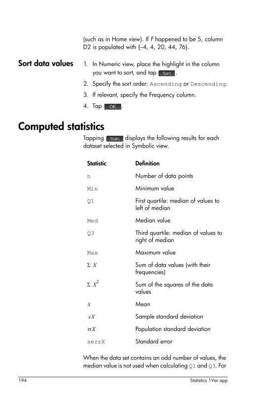
194 Statistics 1Var app
(such as in Home view). If F happened to be 5, column D2 is populated with {–4, 4, 20, 44, 76}.
Sort data values 1. In Numeric view, place the highlight in the column you want to sort, and tap .
2. Specify the sort order: Ascending or Descending.
3. If relevant, specify the Frequency column.
4. Tap .
Computed statisticsTapping displays the following results for each dataset selected in Symbolic view.
When the data set contains an odd number of values, the median value is not used when calculating Q1 and Q3. For
Statistic Definition
n Number of data points
Min Minimum value
Q1 First quartile: median of values to left of median
Med Median value
Q3 Third quartile: median of values to right of median
Max Maximum value
Sum of data values (with their frequencies)
Sum of the squares of the data values
Mean
Sample standard deviation
Population standard deviation
serrX Standard error
X
X2
x
sX
X

Statistics 1Var app 195
example, for the data set {3,5,7,8,15,16,17}only the first three items—3, 5, and 7—are used to calculate Q1, and only the last three terms—5, 16, and 17—are used to calculate Q3.
PlottingYou can plot:
• Histograms
• Box-and-Whisker plots
• Normal Probability plots
• Line plots
• Bar graphs
• Pareto charts
Once you have entered your data and defined your data set, you can plot your data. You can plot up to five box-and-whisker plots at a time; however, with the other types, you can only plot one at a time.
To plot statistical data
1. In the Symbolic view, select the data sets you want to plot.
2. From the Plotn menu, s elect the plot type.
3. For any plot, but especially for a histogram, adjust the plotting scale and range in the Plot Setup view. If you find histogram bars too fat or too thin, you can adjust them by changing the HWIDTH setting. (See “Setting up the plot (Plot Setup view)” on page 197.)
4. Press P. If the scaling is not to your liking, press V and select Autoscale.
Autoscale can be relied upon to give a good starting scale which can then be adjusted in the Plot Setup view.

196 Statistics 1Var app
Plot types
Histogram The first set of numbers below the plot indicate where the cursor is. In the example at the right, the cursor is between 5 and 6 but not including 6), and the frequency for that range is 6. The data set is as defined by H3 in Symbolic view. You can see information about other ranges by pressing >or <.
Box-and-Whisker plot
The left whisker marks the minimum data value. The box marks the first quartile, the median, and the third quartile. The right whisker marks the maximum data value. The numbers below the plot give the statistic at the cursor. You can see other statistics by pressing >or <.
Normal probability plot
The normal probability plot is used to determine whether or not sample data is more or less normally distributed. The more linear the data appear, the more likely that the data is normally distributed.
Line plot The line plot connects points of the form (x, y), where x is the row number of the data point and y is its value.

Statistics 1Var app 197
Bar graph The bar graph shows the value of a data point as a vertical bar placed along the x-axis at the row number of the data point.
Pareto chart A pareto chart places the data in descending order and displays each with its percentage of the whole.
Setting up the plot (Plot Setup view)The Plot Setup view (SP) enables you to specify many of the same plotting parameters as other apps (such as X Rng and Y Rng). There are two settings unique to the Statistics 1Var app:
Histogram width H Width enables you to specify the width of a histogram bar. This determines how many bars will fit in the display, as well as how the data is distributed (that is, how many values each bar represents).
Histogram range H Rng enables you to specify the range of values for a set of histogram bars. The range runs from the left edge of the leftmost bar to the right edge of the rightmost bar. You can limit the range to exclude any values you suspect are outliers.
Exploring the graphThe Plot view (P) has zooming and tracing options, as well as coordinate display. The Autoscale option is available from the View menu (V) as well as the menu.The View menu also enables you to view graphs in split-screen mode (as explained on page 81).

198 Statistics 1Var app
Plot view: buttons menu itemsThe menu items you can tap on in Plot view are:
Button Purpose
Displays the Zoom menu.
Turns trace mode on or off. See “Zoom” on page 90.)
Displays the definition of the current statistical plot.
Shows or hides the menu.

Statistics 2Var app 199
10
Statistics 2Var app
The Statistics 2Var app can store up to ten data sets at one time. It can perform two-variable statistical analysis of one or more sets of data.
The Statistics 2Var app starts with the Numeric view which is used to enter data. The Symbolic view is used to specify which columns contain data and which column contains frequencies.
You can also compute statistics in Home and in the Spreadsheet app.
The values computed in the Statistics 2Var app are saved in variables. These can be referenced in Home view and in other apps.
Getting started with the Statistics 2Var appThe following example uses the advertising and sales data in the table below. In the example, you will enter the data, compute summary statistics, fit a curve to the data, and predict the effect of more advertising on sales.
Advertising minutes (independent, x)
Resulting sales ($) (dependent, y)
2 1400
1 920
3 1100
5 2265
5 2890
4 2200

200 Statistics 2Var app
Open the Statistics 2Var app
1. Open the Statistics 2Var app:
I Select Statistics
2Var.
Enter data 2. Enter the advertising minutes data in column C1:
2E1E3E5E5E4E
3. Enter the resulting sales data in column C2:
1400E920E1100E2265E2890E2200E
Choose data columns and fit
In Symbolic view, you can define up to five analyses of two-variable data, named S1 to S5. In this example, we will define just one: S1. The process involves choosing data sets and a fit type.
4. Specify the columns that contain the data you want to analyze:
Y
In this case, C1 and C2 appear by default. But you could have entered your data into columns other than C1 and C2.

Statistics 2Var app 201
5. Select a fit:
From the Type 1 field select a fit. In this example, select Linear.
6. If you want to choose a color for the graph of the data in Plot view, see “Choose a color for plots” on page 74.
7. If you have more than one analysis defined in Symbolic view, deselect any analysis you are not currently interested in.
Explore statistics 8. Find the correlation, r, between advertising time and sales:
M
The correlation is r=0.8995…
9. Find the mean advertising time ( ).
The mean advertising time,
, is 3.33333… minutes.
x
x

202 Statistics 2Var app
10. Find the mean sales ( ).
The mean sales, , is approximately $1,796.
Press to return to Numeric view.
Setup plot 11. Change the plotting range to ensure that all the data points are plotted (and to select a different data-point indicator, if you wish).
SP(Setup)\100 E4000 E
Plot the graph 12. Plot the graph.
P
Notice that the regression curve (that is, a curve to best fit the data points) is plotted by default.
Display the equation
13. Return to the Symbolic view.
Y
Note the expression in the Fit1 field. It shows that the slope
y
y

Statistics 2Var app 203
(m) of the regression line is 425.875 and the y-intercept (b) is 376.25.
Predict values Let’s now predict the sales figure if advertising were to go up to 6 minutes.
14. Return to the Plot view:
P
The trace option is active by default. This option will move the cursor from data point to data point as you press > or <. As you move from data point to data point, the corresponding x- and y-values appear at the bottom of the screen. In this example, the x-axis represents minutes of advertising and the y-axis represents sales.
However, there is no data point for 6 minutes. Thus we cannot move the cursor to x = 6. Instead, we need to predict what y will be when x = 6, based on the data we do have. To do that, we need to trace the regression curve, not the data points we have.
15. Press \ or = to set the cursor to trace the regression line rather than the data points.
The cursor jumps from whatever data point it was on to the regression curve.
16. Repeatedly press > until x = 6.
If the x-value is not shown at the bottom left of the screen, tap .
When you reach x = 6, you will see that the PREDY value (also displayed at the bottom of the screen)

204 Statistics 2Var app
reads 2931.5. Thus the model predicts that sales would rise to $2,931.50 if advertising were increased to 6 minutes.
T i p You could use the same tracing technique to predict—although roughly—how many minutes of advertising you would need to gain sales of a specified amount. However, a more accurate method is available: return to Home view and enter Predx(s) where s is the sales figure. Predy and Predx are app functions. They are discussed in detail in “Statistics 2Var app functions” on page 331.
Entering and editing statistical dataEach column in Numeric view is a dataset and is represented by a variable named C0 to C9. There are three ways to get data into a column:
• Go to Numeric view and enter the data directly. See “Getting started with the Statistics 2Var app” on page 199 for an example.
• Go to Home view and copy the data from a list. For example, if you enter L1 C1 in Home view, the items in list L1 are copied into column C1 in the Statistics 1Var app.
• Go to Home view and copy the data from a the Spreadsheet app. For example, suppose the data of interest is in A1:A10 in the Spreadsheet app and you want to copy it into column C7. With the Statistics 2Var app open, return to Home view and enter Spreadsheet.A1:A10 C7 E.
T N o t e A data column must have at least four data points to provide valid two-variable statistics.
Whichever method you use, the data you enter is automatically saved. You can leave this app and come back to it later. You will find that the data you last entered is still available.
After entering the data, you must define data sets—and the way they are to be plotted—in Symbolic view.

Statistics 2Var app 205
Numeric view menu itemsThe buttons you can tap on in Numeric view are:
Edit a data set In Numeric view, highlight the data to change, type a new value, and press E. You can also highlight the data, tap , make your change, and tap .
Delete data • To delete a data item, highlight it and press C. The values below the deleted cell will scroll up one row.
• To delete a column of data, highlight an entry in that column and press SJ(Clear). Select the column and tap .
• To delete all data in every column, press SJ (Clear), select All columns, and tap .
Insert data Highlight the cell below where you want to insert a value. Tap and enter the value.
Button Purpose
Copies the highlighted item to the entry line.
Inserts a new cell above the highlighted cell (and gives it a value of 0).
Opens an input form for you to choose to sort the data in various ways.
Displays a menu for you to choose the small font, medium font, or large font.
Opens an input form for you to create a sequence based on an expression, and to store the result in a specified data column. See “Generating data” on page 193.
Calculates statistics for each data set selected in Symbolic view. See “Computed statistics” on page 208.
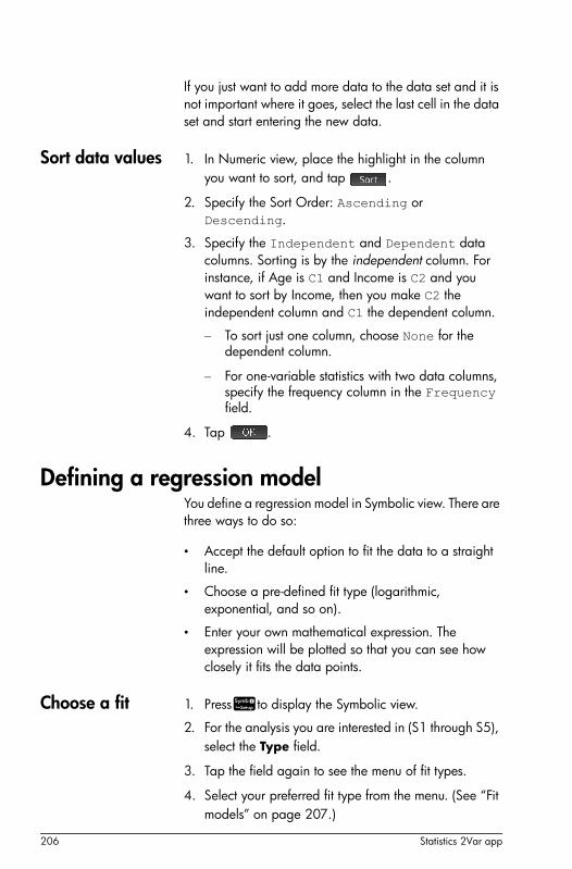
206 Statistics 2Var app
If you just want to add more data to the data set and it is not important where it goes, select the last cell in the data set and start entering the new data.
Sort data values 1. In Numeric view, place the highlight in the column you want to sort, and tap .
2. Specify the Sort Order: Ascending or Descending.
3. Specify the Independent and Dependent data columns. Sorting is by the independent column. For instance, if Age is C1 and Income is C2 and you want to sort by Income, then you make C2 the independent column and C1 the dependent column.
– To sort just one column, choose None for the dependent column.
– For one-variable statistics with two data columns, specify the frequency column in the Frequency field.
4. Tap .
Defining a regression modelYou define a regression model in Symbolic view. There are three ways to do so:
• Accept the default option to fit the data to a straight line.
• Choose a pre-defined fit type (logarithmic, exponential, and so on).
• Enter your own mathematical expression. The expression will be plotted so that you can see how closely it fits the data points.
Choose a fit 1. PressYto display the Symbolic view.
2. For the analysis you are interested in (S1 through S5), select the Type field.
3. Tap the field again to see the menu of fit types.
4. Select your preferred fit type from the menu. (See “Fit models” on page 207.)
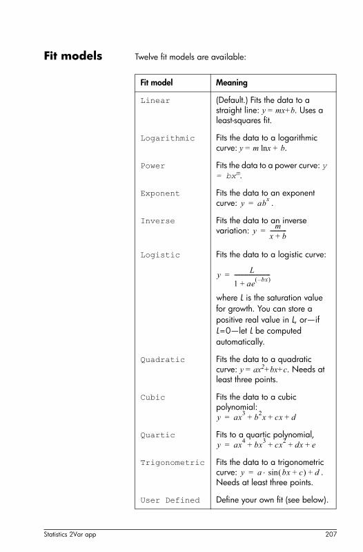
Statistics 2Var app 207
Fit models Twelve fit models are available:
Fit model Meaning
Linear (Default.) Fits the data to a straight line: y = mx+b. Uses a least-squares fit.
Logarithmic Fits the data to a logarithmic curve: y = m lnx + b.
Power Fits the data to a power curve: y = bxm.
Exponent Fits the data to an exponent curve: .
Inverse Fits the data to an inverse variation:
Logistic Fits the data to a logistic curve:
where L is the saturation value for growth. You can store a positive real value in L, or—if L=0—let L be computed automatically.
Quadratic Fits the data to a quadratic curve: y = ax2+bx+c. Needs at least three points.
Cubic Fits the data to a cubic polynomial:
Quartic Fits to a quartic polynomial,
Trigonometric Fits the data to a trigonometric curve: . Needs at least three points.
User Defined Define your own fit (see below).
y abx
=
ym
x b+------------=
yL
1 aebx–
+--------------------------=
y ax3
b2x cx d+ + +=
y ax4
bx3
cx2
dx e+ + + +=
y a bx c+ sin d+=

208 Statistics 2Var app
To define your own fit
1. PressYto display the Symbolic view.
2. For the analysis you are interested in (S1 through S5), select the Type field.
3. Tap the field again to see a menu of fit types.
4. Select User Defined from the menu.
5. Select the corresponding Fitn field.
6. Enter an expression and press E. The independent variable must be X, and the expression must not contain any unknown variables. Example:
. Note that in this app, variables must be entered in uppercase.
Computed statisticsWhen you tap , three sets of statistics become available. By default, the statistics involving both the independent and dependent columns are shown. Tap
to see the statistics involving just the independent column or to display the statistics derived from the dependent column. Tap to return to the default view. The tables below describe the statistics displayed in each view.
The statistics computed when you tap are:
1.5 xcos 0.3 xsin+
Statistic Definition
n The number of data points.
r Correlation coefficient of the independent and dependent data columns, based only on the linear fit (regardless of the fit type chosen). Returns a value between –1 and 1, where 1 and –1 indicate best fits.
R2 The coefficient of determination, that is, the square of the correlation coefficient. The value of this statistics is dependent on the Fit type chosen. A measure of 1 indicates a perfect fit.

Statistics 2Var app 209
The statistics displayed when you tap are:
The statistics displayed when you tap are:
sCOV Sample covariance of independent and dependent data columns.
COV Population covariance of independent and dependent data columns.
XY Sum of all the individual products of of x and y.
Statistic Definition (Continued)
Statistic Definition
Mean of x- (independent) values.
X Sum of x-values.
X2 Sum of x2-values.
sX The sample standard deviation of the independent column.
X The population standard deviation of the independent column.
serrX the standard error of the independent column
x
Statistic Definition
Mean of y- (dependent) values.
Y Sum of y-values.
Y2 Sum of y2-values.
sY The sample standard deviation of the dependent column.
Y The population standard deviation of the dependent column.
serrY The standard error of the dependent column.
y

210 Statistics 2Var app
Plotting statistical dataOnce you have entered your data, selected the data set to analyze and specified your fit model, you can plot your data. You can plot up to five scatter plots at a time.
1. In Symbolic view, select the data sets you want to plot.
2. Make sure that the full range of your data will be plotted. You do this by reviewing (and adjusting, if necessary), the X Rng and Y Rng fields in Plot Setup view. (SP).
3. PressP.
If the data set and regression line are not ideally positioned, Press V and select Autoscale. Autoscale can be relied upon to give a good starting scale which can then be adjusted later in the Plot Setup view.
Tracing a scatter plot
The figures below the plot indicate that the cursor is at the second data point of S1, at ((2, 1400). Press>to move to the next data point and display information about it.
Note: if you find that the tracer cursor is moving along the regression line rather than from data point to data point, press = or \ to select the points and not the line.
Tracing a curve If the regression line is not showing, tap . The coordinates of the tracer cursor are shown at the bottom of the screen. (If they are not visible, tap .)
Note: if you find that the tracer cursor is moving between the data points rather than along the regression line, press = or \ to select the line and not the points.
Tap to display the data sets that being represented by of the regression line.

Statistics 2Var app 211
PressYto see the equation of the regression line in Symbolic view.
If the equation is too wide for the screen, select it and press .
The example above shows that the slope of the regression line (m) is 425.875 and the y-intercept (b) is 376.25.
Plot view: menu itemsThe menu items in Plot view are:
Plot setupAs with all the apps that provide a plotting feature, he Plot Setup view—SP (Setup)—enables you to set the range and appearance of Plot view. The common settings available are discussed in “Common operations in Plot Setup view” on page 86. The Plot Setup view in the Statistics 2Var app has two additional settings:
Button Purpose
Displays the Zoom menu.
Turns trace mode on or off.
Shows or hides a curve that best fits the data points according to the selected regression model.
Enables you to specify a value on the regression line to jump to (or a data point to jump to if your cursor is on a data point rather than on the regression line). You might need to press = or \ to move the cursor to the object of interest: the regression line or the data points.
Shows or hides the menu buttons.

212 Statistics 2Var app
Plotting mark Page 1 of the Plot Setup view has fields namedS1MARK through S5MARK. These fields enable you to specify one of five symbols to use to represent the data points in each data set. This will help you distinguish data sets in Plot view if you have chosen to plot more than one.
Connect Page 2 of the Plot Setup view has a Connect field. If you choose this option, straight lines join the data points in Plot view.
Predicting valuesPredX is a function that predicts a value for X given a value for Y. Likewise, PredY is a function that predicts a value for Y given a value for X. In both cases, the prediction is based on the equation that best fits the data according to the specified fit type.
You can predict values in the Plot view of the Statistics 2Var app and also in Home view.
In Plot view 1. In the Plot view, tap to display the regression curve for the data set (if it is not already displayed).
2. Make sure the trace cursor is on the regression curve. (Press = or \ if it is not.)
3. Press > or <. The cursor moves along the regression curve and the corresponding X and Y values are displayed across the bottom of the screen. (If these values are not visible, tap .)
You can force the cursor to a specific X value by tapping , entering the value and tapping . The cursor
jumps to the specified point on the curve.
In Home view
If the Statistics 2Var app is the active app, you can also predict X and Y values in the Home view.
• Enter PredX(Y) E to predict the X value for the specified Y value.
• Enter PredY(X) E to predict the Y value for the specified X value.
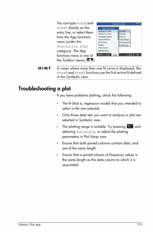
Statistics 2Var app 213
You can type PredX and PredY directly on the entry line, or select them from the App functions menu (under the Statistics 2Var category). The App functions menu is one of the Toolbox menus (D).
H I N T In cases where more than one fit curve is displayed, the PredX and PredY functions use the first active fit defined in the Symbolic view.
Troubleshooting a plotIf you have problems plotting, check the following:
• The fit (that is, regression model) that you intended to select is the one selected.
• Only those data sets you want to analyze or plot are selected in Symbolic view.
• The plotting range is suitable. Try pressing V and selecting Autoscale, or adjust the plotting parameters in Plot Setup view.
• Ensure that both paired columns contain data, and are of the same length.
• Ensure that a paired column of frequency values is the same length as the data column to which it is associated.

214 Statistics 2Var app
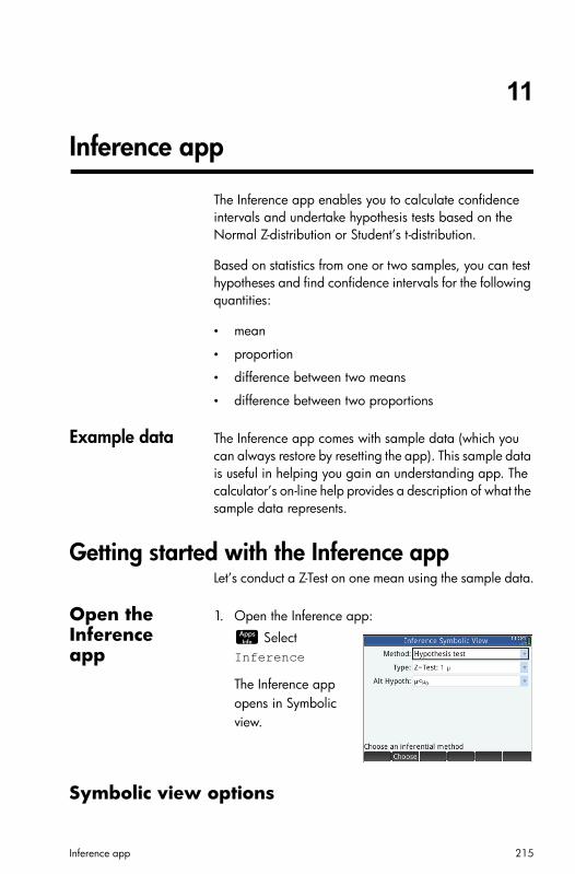
Inference app 215
11
Inference app
The Inference app enables you to calculate confidence intervals and undertake hypothesis tests based on the Normal Z-distribution or Student’s t-distribution.
Based on statistics from one or two samples, you can test hypotheses and find confidence intervals for the following quantities:
• mean
• proportion
• difference between two means
• difference between two proportions
Example data The Inference app comes with sample data (which you can always restore by resetting the app). This sample data is useful in helping you gain an understanding app. The calculator’s on-line help provides a description of what the sample data represents.
Getting started with the Inference appLet’s conduct a Z-Test on one mean using the sample data.
Open the Inference app
1. Open the Inference app:
I Select Inference
The Inference app opens in Symbolic view.
Symbolic view options

216 Inference app
The table below summarizes the options available in Symbolic view for the two inference methods: hypothesis test and confidence interval.
If you choose one of the hypothesis tests, you can choose an alternative hypothesis to test against the null hypothesis. For each test, there are three possible choices for an alternative hypothesis based on a quantitative comparison of two quantities. The null hypothesis is always that the two quantities are equal. Thus, the alternative hypotheses cover the various cases for the two quantities being unequal: <, >, and .
Hypothesis Test Confidence Interval
Z-Test: 1 , the Z-Test on one mean
Z-Int: 1 , the confidence interval for one mean, based on the Normal distribution
Z-Test: 1 – 2, the Z-Test on the difference between two means
Z-Int: 1 – 2, the confidence interval for the difference between two means, based on the Normal distribution
Z-Test: 1 , the Z-Test on one proportion
Z-Int: 1 , the confidence interval for one proportion, based on the Normal distribution
Z-Test: 1– 2, the Z-Test on the difference between two proportions
Z-Int: 1– 2, the confidence interval for the difference between two proportions, based on the Normal distribution
T-Test: 1 , the T-Test on one mean
T-Int: 1 , the confidence interval for one mean, based on the Student’s t-distribution
T-Test: 1 – 2, the T-Test on the difference between two means
T-Int: 1 – 2, the confidence interval for the difference between two means, based on the Student’s t-distribution

Inference app 217
In this section, we will conduct a Z-Test on one mean on the example data to illustrate how the app works.
Select the inference method
2. Hypothesis Test is the default inference method. If it is not selected, tap on the Method field and select it.
3. Choose the type of test. In this case, select Z–Test: 1 from the Type menu.
4. Select an alternative hypothesis. In this case, select from the Alt Hypoth menu.
Enter data 5. Go to Numeric view to see the sample data.
M
The table below describes the fields in this view for the sample data.
0
Field name
Definition
Sample meanx

218 Inference app
We’ll leave the data as it is for now, but the Numeric view is where you add the data you are particularly interested in.
Display the test results
6. Display the test results:
The test distribution value and its associated probability are displayed, along with the critical value(s) of the test and the associated critical value(s) of the statistic.
Tap to return to Numeric view.
Plot the test results
7. Display a graphical view of the test results:
P
The graph of the distribution is displayed, with the test Z-value marked. The corresponding X-value is also shown.
Tap to see the critical Z-value. With the alpha level showing, you can press \ or = to decrease or increase the -level.
n Sample size
Assumed population mean
Population standard deviation
Alpha level for the test
Field name
Definition (Continued)
0
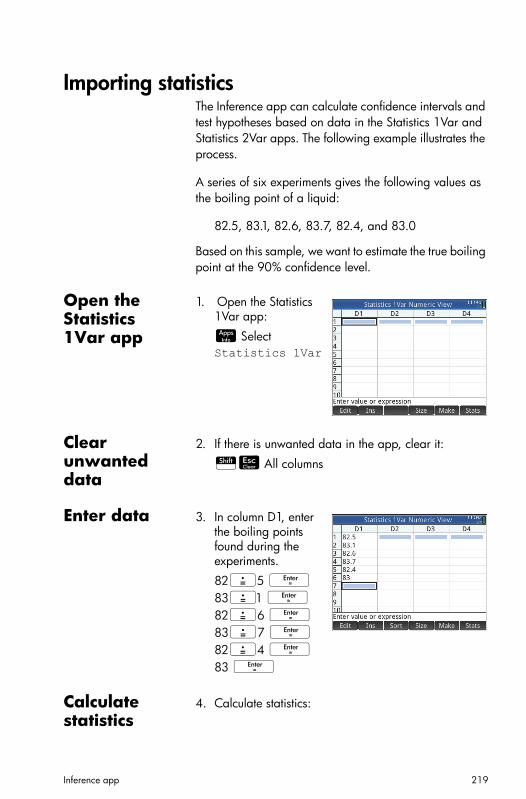
Inference app 219
Importing statisticsThe Inference app can calculate confidence intervals and test hypotheses based on data in the Statistics 1Var and Statistics 2Var apps. The following example illustrates the process.
A series of six experiments gives the following values as the boiling point of a liquid:
82.5, 83.1, 82.6, 83.7, 82.4, and 83.0
Based on this sample, we want to estimate the true boiling point at the 90% confidence level.
Open the Statistics 1Var app
1. Open the Statistics 1Var app:
I Select Statistics 1Var
Clear unwanted data
2. If there is unwanted data in the app, clear it:
SJ All columns
Enter data 3. In column D1, enter the boiling points found during the experiments.
82.5 E 83.1 E
82.6 E 83.7 E 82.4 E83 E
Calculate statistics
4. Calculate statistics:

220 Inference app
The statistics calculated will now be imported into the Inference app.
5. Tap to close the statistics window.
Open the Inference app
6. Open the Inference app and clear the current settings.
I Select Inference
SJ
Select inference method and type
7. Tap on the Method field and select Confidence Interval.
8. Tap on Type and select T-Int: 1
Import the data
9. Open Numeric view:
M
10.Specify the data you want to import:
Tap .

Inference app 221
11. From the App field select the statistics app that has the data you want to import.
12. In the Column field specify the column in that app where the data is stored. (D1 is the default.)
13. Tap .14. Specify a 90%
confidence interval in the C field.
Display results numerically
15. Display the confidence interval in Numeric view:
16. Return to Numeric view:
Display results graphically
17. Display the confidence interval in Plot view.
P
You can see that we can be 90% confident that the true boiling point lies between 82.4822… and 83.2843…
Hypothesis testsYou use hypothesis tests to test the validity of hypotheses about the statistical parameters of one or two populations.

222 Inference app
The tests are based on statistics of samples of the populations.
The HP Prime hypothesis tests use the Normal Z-distribution or the Student’s t-distribution to calculate probabilities.
One-Sample Z-Test
Menu name Z-Test: 1
On the basis of statistics from a single sample, this test measures the strength of the evidence for a selected hypothesis against the null hypothesis. The null hypothesis is that the population mean equals a specified value, .
You select one of the following alternative hypotheses against which to test the null hypothesis:
H1: <0
H1: >0
H1: ≠0
Inputs The inputs are:
Field name Definition
Sample mean
n Sample size
0 Hypothetical population mean
Population standard deviation
Significance level
x

Inference app 223
Results The results are:
Two-Sample Z-Test
Menu name Z-Test: 1 – 2
On the basis of two samples, each from a separate population, this test measures the strength of the evidence for a selected hypothesis against the null hypothesis. The null hypothesis is that the means of the two populations are equal, 0: 1 = 2.
You select one of the following alternative hypotheses to test against the null hypothesis:
H1: 1 <2
H1: 1 >2
H1: 1≠2
Inputs The inputs are:
Result Description
Test Z Z-test statistic
Test Value of associated with the test Z-value
P Probability associated with the Z-Test statistic
Critical Z Boundary value(s) of Z associated with the level that you supplied
Critical Boundary value(s) of required by the value that you supplied
x x
x x
Field name Definition
Sample 1 mean
Sample 2 mean
n1 Sample 1 size
n2 Sample 2 size
x1
x2

224 Inference app
Results The results are:
One-Proportion Z-Test
Menu name Z-Test:
On the basis of statistics from a single sample, this test measures the strength of the evidence for a selected hypothesis against the null hypothesis. The null hypothesis is that the proportion of successes is an assumed value, 0: = 0.
You select one of the following alternative hypotheses against which to test the null hypothesis:
H1: <0
H1: >0
H1: ≠ 0
1 Population 1 standard deviation
2 Population 2 standard deviation
Significance level
Field name Definition (Continued)
Result Description
Test Z Z-Test statistic
Test Difference in the means associ-ated with the test Z-value
P Probability associated with the Z-Test statistic
Critical Z Boundary value(s) of Z associ-ated with the level that you supplied
Critical Difference in the means associ-ated with the level you sup-plied
x
x
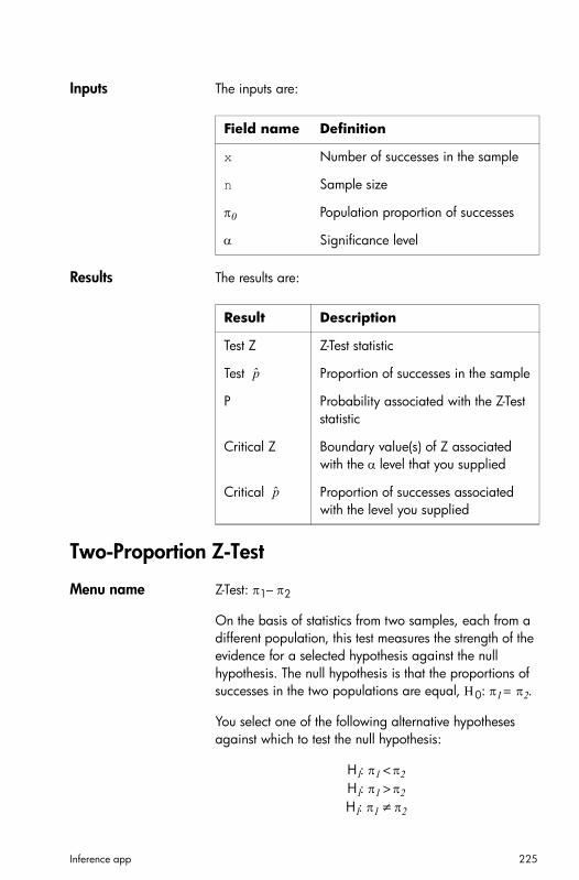
Inference app 225
Inputs The inputs are:
Results The results are:
Two-Proportion Z-Test
Menu name Z-Test: 1– 2
On the basis of statistics from two samples, each from a different population, this test measures the strength of the evidence for a selected hypothesis against the null hypothesis. The null hypothesis is that the proportions of successes in the two populations are equal, 0: 1= 2.
You select one of the following alternative hypotheses against which to test the null hypothesis:
H1: 1 <2
H1: 1 >2
H1: 1≠2
Field name Definition
x Number of successes in the sample
n Sample size
0 Population proportion of successes
Significance level
Result Description
Test Z Z-Test statistic
Test Proportion of successes in the sample
P Probability associated with the Z-Test statistic
Critical Z Boundary value(s) of Z associated with the level that you supplied
Critical Proportion of successes associated with the level you supplied
p̂
p̂

226 Inference app
Inputs The inputs are:
Results The results are:
Field name Definition
x1 Sample 1 success count
x2 Sample 2 success count
n1 Sample 1 size
n2 Sample 2 size
Significance level
Result Description
Test Z Z-Test statistic
Test Difference between the proportions of successes in the two samples that is associated with the test Z-value
P Probability associated with the Z-Test statistic
Critical Z Boundary value(s) of Z associated with the level that you supplied
Critical Difference in the proportion of successes in the two samples associated with the level you supplied
p̂
p̂
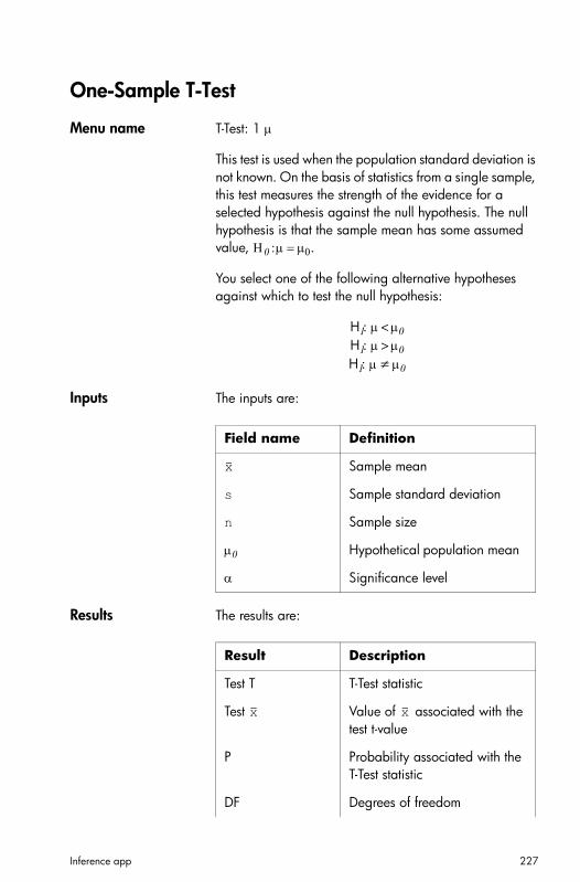
Inference app 227
One-Sample T-Test
Menu name T-Test: 1
This test is used when the population standard deviation is not known. On the basis of statistics from a single sample, this test measures the strength of the evidence for a selected hypothesis against the null hypothesis. The null hypothesis is that the sample mean has some assumed value, 0.
You select one of the following alternative hypotheses against which to test the null hypothesis:
H1: <0
H1: >0
H1: ≠0
Inputs The inputs are:
Results The results are:
Field name Definition
Sample mean
s Sample standard deviation
n Sample size
0 Hypotheticalpopulation mean
Significance level
x
Result Description
Test T T-Test statistic
Test Value of associated with the test t-value
P Probability associated with theT-Test statistic
DF Degrees of freedom
x x

228 Inference app
Two-Sample T-Test
Menu name T-Test: 1 – 2
This test is used when the population standard deviation is not known. On the basis of statistics from two samples, each sample from a different population, this test measures the strength of the evidence for a selected hypothesis against the null hypothesis. The null hypothesis is that the two populations means are equal, 0: = .
You select one of the following alternative hypotheses against which to test the null hypothesis:
H1: 1 <2
H1: 1 >2
H1: 1≠2
Inputs The inputs are:
Critical T Boundary value(s) of T associated with the level that you supplied
Critical Boundary value(s) of required by the value that you supplied
Result Description (Continued)
x x
Field name
Definition
Sample 1 mean
Sample 2 mean
s1 Sample 1 standard deviation
s2 Sample 2 standard deviation
n1 Sample 1 size
n2 Sample 2 size
Significance level
x1
x2

Inference app 229
Results The results are:
Confidence intervalsThe confidence interval calculations that the HP Prime can perform are based on the Normal Z-distribution or Student’s t-distribution.
One-Sample Z-Interval
Menu name Z-Int:
This option uses the Normal Z-distribution to calculate a confidence interval for , the true mean of a population, when the true population standard deviation, , is known.
Inputs The inputs are:
Pooled Check this option to pool samples based on their standard deviations
Field name
Definition
Result Description
Test T T-Test statistic
Test Difference in the means associated with the test t-value
P Probability associated with the T-Test statistic
DF Degrees of freedom
Critical T Boundary values of T associated with the level that you supplied
Critical Difference in the means associated with the level you supplied
x
x
Field name
Definition
Sample meanx

230 Inference app
Results The results are:
Two-Sample Z-Interval
Menu name Z-Int: 1 – 2
This option uses the Normal Z-distribution to calculate a confidence interval for the difference between the means of two populations, –, when the population standard deviations, 1 and 2, are known.
Inputs The inputs are:
n Sample size
Population standard deviation
C Confidence level
Field name
Definition
Result Description
C Confidence level
Critical Z Critical values for Z
Lower Lower bound for
Upper Upper bound for
Field name
Definition
Sample 1 mean
Sample 2 mean
n1 Sample 1 size
n2 Sample 2 size
1 Population 1 standard deviation
2 Population 2 standard deviation
x1
x2

Inference app 231
Results The results are:
One-Proportion Z-Interval
Menu name Z-Int: 1
This option uses the Normal Z-distribution to calculate a confidence interval for the proportion of successes in a population for the case in which a sample of size n has a number of successes x.
Inputs The inputs are:
Results The results are:
C Confidence level
Field name
Definition
Result Description
C Confidence level
Critical Z Critical values for Z
Lower Lower bound for
Upper Upper bound for
Field name
Definition
x Sample success count
n Sample size
C Confidence level
Result Description
C Confidence level
Critical Z Critical values for Z
Lower Lower bound for

232 Inference app
Two-Proportion Z-IntervalMenu name Z-Int: 1 – 2
This option uses the Normal Z-distribution to calculate a confidence interval for the difference between the proportions of successes in two populations.
Inputs The inputs are:
Results The results are:
One-Sample T-Interval
Menu name T-Int: 1
This option uses the Student’s t-distribution to calculate a confidence interval for , the true mean of a population,
Upper Upper bound for
Result Description
Field name
Definition
Sample 1 success count
Sample 2 success count
n1 Sample 1 size
n2 Sample 2 size
C Confidence level
x1
x2
Result Description
C Confidence level
Critical Z Critical values for Z
Lower Lower bound for
Upper Upper bound for

Inference app 233
for the case in which the true population standard deviation, , is unknown.
Inputs The inputs are:
Results The results are:
Two-Sample T-Interval
Menu name T-Int: 1 – 2
This option uses the Student’s t-distribution to calculate a confidence interval for the difference between the means of two populations, 1 – 2, when the population standard deviations, 1and 2, are unknown.
Inputs The inputs are:
Field name
Definition
Sample mean
s Sample standard deviation
n Sample size
C Confidence level
x
Result Description
C Confidence level
DF Degrees of freedom
Critical T Critical values for T
Lower Lower bound for
Upper Upper bound for
Result Definition
Sample 1 mean
Sample 2 mean
x1
x2
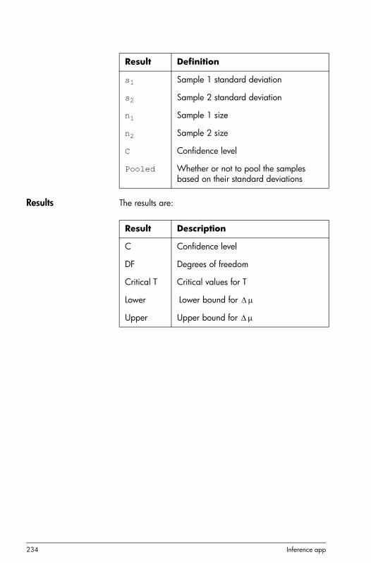
234 Inference app
Results The results are:
s1 Sample 1 standard deviation
s2 Sample 2 standard deviation
n1 Sample 1 size
n2 Sample 2 size
C Confidence level
Pooled Whether or not to pool the samples based on their standard deviations
Result Definition
Result Description
C Confidence level
DF Degrees of freedom
Critical T Critical values for T
Lower Lower bound for
Upper Upper bound for

Solve app 235
12
Solve app
The Solve app enables you to define up to ten equations or expressions each with as many variables as you like. You can solve a single equation or expression for one of its variables, based on a seed value. You can also solve a system of equations (linear or non-linear), again using seed values.
Note the differences between an equation and an expression:
• An equation contains an equals sign. Its solution is a value for the unknown variable that makes both sides of the equation have the same value.
• An expression does not contain an equals sign. Its solution is a root, a value for the unknown variable that makes the expression have a value of zero.
For brevity, the term equation in this chapter will cover both equations and expressions.
Solve works only with real numbers.
Getting started with the Solve appThe Solve app uses the customary app views: Symbolic, Plot and Numeric described in chapter 4.
For a description of the menu buttons available in this app, see:
• “Symbolic view: Summary of menu buttons” on page 76
• “Plot view: Summary of menu buttons” on page 86, and
• “Numeric view: Summary of menu buttons” on page 94
One equationSuppose you want to find the acceleration needed to increase the speed of a car from 16.67 m/s (60 kph) to 27.78 m/s (100 kph) over a distance of 100 m.
The equation to solve is:

236 Solve app
V 2 = U2 +2AD.
where V = final speed, U = initial speed, A = acceleration needed, and D = distance.
Open the Solve app
1. Open the Solve app.
I Select Solve
The Solve app starts in Symbolic view, where you specify the equation to solve.
N O T E In addition to the built-in variables, you can use one or more variables you created yourself (either in Home view or in the CAS). For example, if you’ve created a variable called ME, you could include it in an equation such as this: Y 2 = G2 + ME.
Functions defined in other apps can also be referenced in the Solve app. For example, if you have defined F1(X) to be X2 +10 in the Function app, you can enter F1(X)=50 in the Solve app to solve the equation X2 + 10 = 50.
Clear the app and define the equation
2. If you have no need for any equations or expressions already defined, press SJ (Clear). Tap to confirm your intention to clear the app.
3. Define the equation.
AVjS.AUj+2AAADE
Enter known variables
4. Display the Numeric view.

Solve app 237
M
Here you specify the values of the known variables, highlight the variable that you want to solve for, and tap .
5. Enter the values for the known variables.
2 7.7 8E1 6.6 7E\1 0 0 E
N O T E Some variables may already have values against them when you display the Numeric view. This occurs if the variables have been assigned values elsewhere. For example, in Home view you might have assigned 10 to variable U: 10 U. Then when you open the Numeric view to solve an equation with U as a variable, 10 will be the default value for U. This also occurs if a variable has been given a value in some previous calculation (in an app or program).
To reset all pre-populated variables to zero, press SJ.
Solve the unknown variable
6. Solve for the unknown variable (A).
Move the cursor to the A field and tap .
Therefore, the acceleration needed to increase the speed of a car from 16.67 m/s (60 kph) to 27.78 m/s (100 kph) over a distance of 100 m is approximately 2.4692 m/s2.
The equation for A is (V 2 – U 2)/2D. This is a linear equation. Hence we can conclude that there are no further solutions for A. We can also see this if we plot the equation.
Plot the equation
The Plot view shows one graph for each side of the solved equation. You can choose any of the variables to be the

238 Solve app
independent variable by selecting it in Numeric view. So in this example make sure that A is highlighted.
The current equation is V 2 = U2 +2AD. The plot view will plot two equations, one for each side of the equation. One of these is Y = V 2, with V = 27.78, making Y = 771.7284. This graph will be a horizontal line. The other graph will be Y = U2 +2AD with U =16.67and D =100, making, Y = 200A + 277.8889. This graph is also a line. The desired solution is the value of A where these two lines intersect.
7. Plot the equation for variable A.
V
Select Auto Scale.
Select Both sides of En (where n is the number of the selected equation)
8. Tap and then . Using the cursor
keys, move the trace cursor along either graph until it nears the intersection. Note that the value of A displayed near the bottom left corner of the screen closely matches the value of A you calculated above.
The Plot view provides a convenient way to find an approximation to a solution when you suspect that there are a number of solutions. Move the trace cursor close to the solution (that is, the intersection) of interest to you and then open Numeric view. The solution given in Numeric view will be will be for the solution nearest the trace cursor.
N O T E By dragging a finger horizontally or vertically across the screen, you can quickly see parts of the plot that are initially outside the x and y ranges you set.
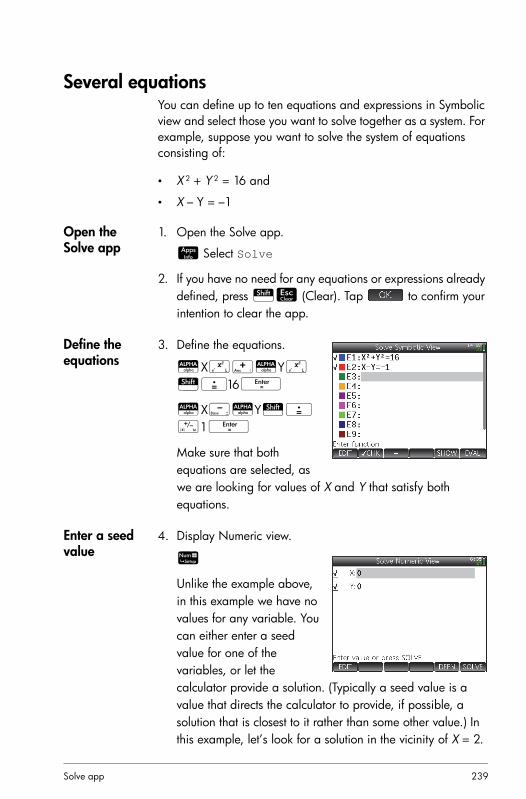
Solve app 239
Several equationsYou can define up to ten equations and expressions in Symbolic view and select those you want to solve together as a system. For example, suppose you want to solve the system of equations consisting of:
• X 2 + Y 2 = 16 and
• X – Y = –1
Open the Solve app
1. Open the Solve app.
I Select Solve
2. If you have no need for any equations or expressions already defined, press SJ (Clear). Tap to confirm your intention to clear the app.
Define the equations
3. Define the equations.
AXj+AYjS.16E
AXwAYS.Q1E
Make sure that both equations are selected, as we are looking for values of X and Y that satisfy both equations.
Enter a seed value
4. Display Numeric view.
M
Unlike the example above, in this example we have no values for any variable. You can either enter a seed value for one of the variables, or let the calculator provide a solution. (Typically a seed value is a value that directs the calculator to provide, if possible, a solution that is closest to it rather than some other value.) In this example, let’s look for a solution in the vicinity of X = 2.

240 Solve app
5. Enter the seed value in the X field:
2
The calculator will provide one solution (if there is one) and you will not be alerted if there are multiple solutions. Vary the seed values to find other potential solutions.
6. Select the variables you want solutions for. In this example we want to find values for both X and Y, so make sure that both variables are selected.
Note too that if you have more than two variables, you can enter seed values for more than one of them.
Solve the unknown variables
7. Tap to find a solution near X = 2 that satisfies each selected equation. Solutions, if found, are displayed beside each selected variable.
LimitationsYou cannot plot equations if more than one is selected in Symbolic view.
The HP Prime will not alert you to the existence of multiple solutions. If you suspect that another solution exists close to a particular value, repeat the exercise using that value as a seed. (In the example just discussed, you will find another solution if you enter –3 as the seed value for X.)
In some situations, the Solve app will use a random number seed in its search for a solution. This means that is it not always predictable which seed will lead to which solution when there are multiple solutions.
Solution informationWhen you are solving a single equation, the button appears on the menu after you tap . Tapping
Solve app 241
displays a message giving you some information about the solutions found (if any). Tap to clear the message.
Message Meaning
Zero The Solve app found a point where both sides of the equation were equal, or where the expression was zero (a root), within the calculator's 12-digit accuracy.
Sign Reversal
Solve found two points where the two sides of the equation have opposite signs, but it cannot find a point in between where the value is zero. Similarly, for an expression, where the value of the expression has different signs but is not precisely zero. This might be be cause either the two points are neighbours (they differ by one in the twelfth digit), or the equation is not real-valued between the two points. Solve returns the point where the value or difference is closer to zero. If the equation or expression is continuously real, this point is Solve’s best approximation of an actual solution.
Extremum Solve found a point where the value of the expression approximates a local minimum (for positive values) or maximum (for negative values). This point may or may not be a solution.
Or:
Solve stopped searching at 9.99999999999E499, the largest number the calculator can represent.
Note that the Extremum message indicates that it is highly likely that there is no solution. Use Numeric view to verify this (and note that any values shown are suspect).
Cannot find solution
No values satisfy the selected equation or expression.

242 Solve app
Bad Guess(es)
The initial guess lies outside the domain of the equation. Therefore, the solution was not a real number or it caused an error.
Constant? The value of the equation is the same at every point sampled.
Message Meaning (Continued)
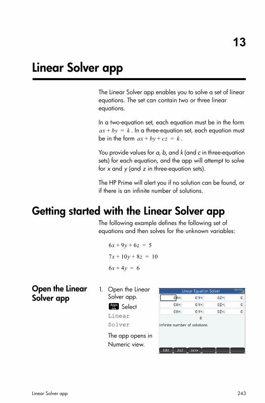
Linear Solver app 243
13
Linear Solver app
The Linear Solver app enables you to solve a set of linear equations. The set can contain two or three linear equations.
In a two-equation set, each equation must be in the form . In a three-equation set, each equation must
be in the form .
You provide values for a, b, and k (and c in three-equation sets) for each equation, and the app will attempt to solve for x and y (and z in three-equation sets).
The HP Prime will alert you if no solution can be found, or if there is an infinite number of solutions.
Getting started with the Linear Solver appThe following example defines the following set of equations and then solves for the unknown variables:
Open the Linear Solver app
1. Open the Linear Solver app.
I Select Linear
Solver
The app opens in Numeric view.
ax by+ k=ax by cz+ + k=
6x 9y 6z+ + 5=
7x 10y 8z+ + 10=
6x 4y+ 6=
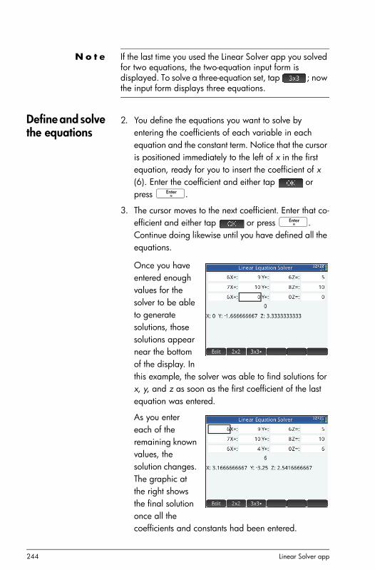
244 Linear Solver app
N o t e If the last time you used the Linear Solver app you solved for two equations, the two-equation input form is displayed. To solve a three-equation set, tap ; now the input form displays three equations.
Define and solve the equations
2. You define the equations you want to solve by entering the coefficients of each variable in each equation and the constant term. Notice that the cursor is positioned immediately to the left of x in the first equation, ready for you to insert the coefficient of x (6). Enter the coefficient and either tap or press E.
3. The cursor moves to the next coefficient. Enter that co-efficient and either tap or press E. Continue doing likewise until you have defined all the equations.
Once you have entered enough values for the solver to be able to generate solutions, those solutions appear near the bottom of the display. In this example, the solver was able to find solutions for x, y, and z as soon as the first coefficient of the last equation was entered.
As you enter each of the remaining known values, the solution changes. The graphic at the right shows the final solution once all the coefficients and constants had been entered.

Linear Solver app 245
Solve a two-by-two system
If the three-equation input form is displayed and you want to solve a two-equation set, tap
.
N o t e You can enter any expression that resolves to a numerical result, including variables. Just enter the name of a variable. For more information on assigning values to variables, see “Storing a value in a variable” on page 39.
Menu itemsThe menu items are:
• : moves the cursor to the entry line where you can add or change a value. You can also highlight a field, enter a value, and press E. The cursor automatically moves to the next field, where you can enter the next value and press E.
• : displays the page for solving a system of 2 linear equations in 2 variables; changes to when active
• : displays the page for solving a system of 3 linear equations in 3 variables; changes to when active

246 Linear Solver app

Parametric app 247
14
Parametric app
The Parametric app enables you to explore parametric equations. These are equations in which both x and y are defined as functions of t. They take the forms and
.
Getting started with the Parametric appThe Parametric app uses the customary app views: Symbolic, Plot and Numeric described in chapter 4.
For a description of the menu buttons available in this app, see:
• “Symbolic view: Summary of menu buttons” on page 76
• “Plot view: Summary of menu buttons” on page 86, and
• “Numeric view: Summary of menu buttons” on page 94
Throughout this chapter, we will explore the parametric equations x(T) = 8sin(T) and y(T) = 8cos(T). These equations produce a circle.
Open the Parametric app
1. Open the Parametric app.
ISelect Parametric
The Parametric app starts in Symbolic view. This is the defining view. It is where you symbolically define (that is, specify) the parametric expressions you want to explore.
x f t =y g t =

248 Parametric app
The graphical and numerical data you see in Plot view and Numeric view are derived from the symbolic functions defined here.
Define the functions
There are 20 fields for defining functions. These are labelled X1(T) through X9(T) and X0(T), and Y1(T) through Y9(T) and Y0(T). Each X function is paired with a Y function.
2. Highlight which pair of functions you want to use, either by tapping on, or scrolling to, one of the pair. If you are entering a new function, just start typing. If you are editing an existing function, tap and make your changes. When you have finished defining or changing the function, press E.
3. Define the two expressions.
8ed?E 8fd?E
Notice how the d key enters whatever variable is relevant to the current app. In the Function app, d enters an X. In the Parametric app it enters a T. In the Polar app, discussed in chapter15, it enters .
4. Decide if you want to:
– give one or more function a custom color when it is plotted
– evaluate a dependent function
– deselect a definition that you don’t want to explore
– incorporate variables, math commands and CAS commands in a definition.
For the sake of simplicity we can ignore these operations in this example. However, they can be useful and are described in detail in “Common operations in Symbolic view” on page 71.

Parametric app 249
Set the angle measure
Set the angle measure to degrees:
5. SY (Settings)
6. Tap the Angle Measure field and select Degrees.
You could also have set the angle measure on the Home Settings screen. However, Home settings are system-wide. By setting the angle measure in an app rather than Home view, you are limiting the setting just to that app.
Set up the plot
7. Open the Plot Setup view:
SP (Setup)
8. Set up the plot by specifying appropriate graphing options. In this example, set the T Rng and T Step fields so that T steps from 0to360 in 5 steps:
Select the 2nd T Rng field and enter:
360 5
Plot the functions
9. Plot the functions:
P

250 Parametric app
Explore the graph
The menu button gives you access to common tools for exploring plots:
: displays a range of zoom options. (The + and w keys can also be used to zoom in and out.)
: when active, enables a tracing cursor to be moved along the contour of the plot (with the coordinates of the cursor displayed at the bottom of the screen).
: specify a T value and the cursor moves to the corresponding x and y coordinates.
: display the functions responsible for the plot.
Detailed information about these tools is provided in “Common operations in Plot view” on page 77.
Typically you would modify a plot by changing its definition in Symbolic view. However, you can modify some plots by changing the Plot Setup parameters. For example, you can plot a triangle instead of a circle simply by changing two plot setup parameters. The definitions in Symbolic view remain unchanged. Here is how it is done:
10. Press SP (Setup).
11. Change T Step to 120.
12. Tap .13. From the Method menu, select Fixed-Step
Segments.
14. Press P.
A triangle is displayed instead of a circle. This is because the new value of T Step makes the points being plotted 120 apart instead of the nearly continuous 5. And by selecting Fixed-Step Segments the points 120° apart are connected with line segments.

Parametric app 251
Display the numeric view
15. Display the Numeric view:
M
16. With the cursor in the T column, type a new value and tap .The table scrolls to the value you entered.
You can also zoom in or out on the independent variable (thereby decreasing or increasing the increment between consecutive values). This and other options are explained in “Common operations in Numeric view” on page 90.
You can see the Plot and Numeric views side by side. See “Combining Plot and Numeric Views” on page 96.

252 Parametric app

Polar app 253
15
Polar app
The Polar app enables you to explore polar equations. Polar equations are equations in which r—the distance a point is from the origin: (0,0)—is defined in terms of , the angle a segment from the point to the origin makes with the polar axis. Such equations take the form .
Getting started with the Polar appThe Polar app uses the six standard app views described in chapter 4, “An introduction to HP apps”, beginning on page 59. That chapter also describes the menu buttons used in the Polar app.
Throughout this chapter, we will explore the expression 5cos(/2)cos()2.
Open the Polar app
1. Open the Polar app:
I Select Polar
The app opens in Symbolic view.
Define the function
There are 10 fields for defining polar functions. These are labelled R1() through R9() and R0().
2. Highlight the field you want to use, either by tapping on it or scrolling to it. If you are entering a new function, just start typing. If you are editing an existing function, tap and make your changes. When you have finished defining or changing the function, press E.
3. Define the expression 5cos(/2)cos()2.
r f =

254 Polar app
5Szfdn2>>fd>jE
Notice how the d key enters whatever variable is relevant to the current app. In this app the relevant variable is .
4. If you wish, choose a color for the plot other than its default. You do this by selecting the colored square to the left of the function set, tapping , and selecting a color from the color-picker.
For more information about adding definitions, modifying definitions, and evaluating dependent definitions in Symbolic view, see “Common operations in Symbolic view” on page 71.
Set angle measure
Set the angle measure to radians:
5. SY (Settings)
6. Tap the Angle Measure field and select Radians.
For more information on the Symbolic Setup view, see “Common operations in Symbolic Setup view” on page 76.
Set up the plot
7. Open the Plot Setup view:
SP (Setup)

Polar app 255
8. Set up the plot by specifying appropriate graphing options. In this example, set the upper limit of the range of the independent variable to 4:
Select the 2nd Rng field and enter 4Sz (
There are numerous ways of configuring the appearance of Plot view. For more information, see “Common operations in Plot Setup view” on page 86.
Plot the expression
9. Plot the expression:
P
Explore the graph
10.Display the Plot view menu.
A number of options appear to help you can explore the graph, such as zoom and trace options. using the trace and zoom options. You can also jump directly to a particular value by entering that value. The Go To screen appears with the number you typed on the entry line. Just tap to accept it. (You could also tap the
button and spwecify the target value.)

256 Polar app
If only one polar equation is plotted, you can see the equation that generated the plot by tapping . If there are several equations plotted, move the tracing cursor to the plot you are interested—by pressing = or \—and then tap .
For more information on exploring plots in Plot view, see “Common operations in Plot view” on page 77.
Display the Numeric view
11. Open the Numeric view:
M
The Numeric view displays a table of values for and R1. If you had specified, and selected, more than one polar function in Symbolic view, a column of evaluations would appear for each one: R2, R3, R4 and so on.
12. With the cursor in the column, type a new value and tap .The table scrolls to the value you entered.
You can also zoom in or out on the independent variable (thereby decreasing or increasing the increment between consecutive values). This and other options are explained in “Common operations in Numeric view” on page 90.
You can see the Plot and Numeric views side by side. See “Combining Plot and Numeric Views” on page 96.

Sequence app 257
16
Sequence app
The Sequence app provides you with various ways to explore sequences.
You can define a sequence named, for example, U1:
• in terms of n
• in terms of U1(n –1)
• in terms of U1(n –2)
• in terms of another sequence, for example, U2(n) or
• in any combination of the above.
You can define a sequence by specifying just the first term and the rule for generating all subsequent terms. However, you will have to enter the second term if the HP Prime is unable to calculate it automatically. Typically if the nth term in the sequence depends on n –2, then you must enter the second term.
The app enables you to create two types of graphs:
• a Stairsteps graph, which plots n on the horizontal axis and Un on the vertical axis
• a Cobweb graph, which plots Un–1 on the horizontal axis and Un on the vertical axis.
Getting started with the Sequence appThe following example explores the well-known Fibonacci sequence, where each term, from the third term on, is the sum of the preceding two terms. In this example, we specify three sequence fields: the first term, the second term and a rule for generating all subsequent terms.
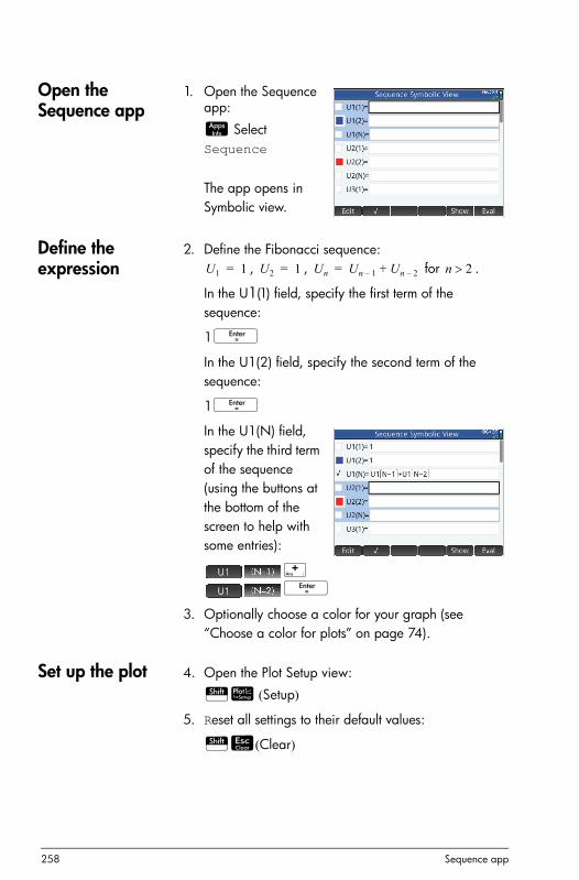
258 Sequence app
Open the Sequence app
1. Open the Sequence app:
I Select Sequence
The app opens in Symbolic view.
Define the expression
2. Define the Fibonacci sequence: , , for .
In the U1(1) field, specify the first term of the sequence:
1E
In the U1(2) field, specify the second term of the sequence:
1E
In the U1(N) field, specify the third term of the sequence (using the buttons at the bottom of the screen to help with some entries):
+E
3. Optionally choose a color for your graph (see “Choose a color for plots” on page 74).
Set up the plot 4. Open the Plot Setup view:
SP (Setup)
5. Reset all settings to their default values:
SJ(Clear)
U1 1= U2 1= Un Un 1– Un 2–+= n 2

Sequence app 259
6. Select Stairstep from the Seq Plot menu.
7. Set the X Rng maximum, and the Y Rng maximum, to 8 (as shown at the right).
Plot the sequence
8. Plot the Fibonacci sequence:
P
9. Return to Plot Setup view (SP) and select Cobweb, from the Seq Plot menu.
10. Plot the sequence:
P
Explore the graph
The button gives you access to common plot-exploration tools, such as:
• Zoom in or out on the plot:
• Trace along a graph:
• Go to a specified N value:
• Display the sequence definition:
These tools are explained in “Common operations in Plot view” on page 77.
Split screen and autoscaling functionality is also available by pressing V.

260 Sequence app
Display Numeric view
11. Display Numeric view:
M
12. With the cursor anywhere in the N column, type a new value and tap
.
The table of values scrolls to the value you entered. You can then see the corresponding value in the sequence. The example at the right shows that the 25th value in the Fibonacci sequence is 75,025.
Explore the table of values
The button gives you access to common table-exploration tools, such as:
• Change the increment between consecutive values:
• Change the size of the font:
• Display the sequence definition:
• Choose the number of sequences to display:
These tools are explained in “Common operations in Numeric view” on page 90.
Split screen and autoscaling functionality is also available by pressing V.

Sequence app 261
Set up the table of values
The Numeric Setup view provides options common to most of the graphing apps. See “Common operations in Numeric Setup view” on page 95 for more information.
Another example: A table of cubesIn the following example, a table of cubes is created. Note that if you are specifying two starting terms (as in the Fibonacci example above) or one (as in the example at the right, the rule that generates the sequence must be placed in the Un(N) field.

262 Sequence app

Finance app 263
17
Finance app
The Finance app enables you to solve time-value-of-money (TVM) and amortization problems. You can use the app to do compound interest calculations and to create amortization tables.
Compound interest is accumulative interest, that is, interest on interest already earned. The interest earned on a given principal is added to the principal at specified compounding periods, and then the combined amount earns interest at a certain rate. Financial calculations involving compound interest include savings accounts, mortgages, pension funds, leases, and annuities.
Getting Started with the Finance appSuppose you finance the purchase of a car with a 5-year loan at 5.5% annual interest, compounded monthly. The purchase price of the car is $19,500, and the down payment is $3,000. First, what are the required monthly payments? Second, what is the largest loan you can afford if your maximum monthly payment is $300? Assume that the payments start at the end of the first period.
1. Start the Finance app.
I Select Finance
The app opens in the Numeric view.
2. In the N field, enter 5 s12 and press E.
Notice that the result of the calculation (60) appears in the field. This is the number of months over a five-year period.

264 Finance app
3. In the I%/YR field, type 5.5—the interest rate—and press E.
4. In PV field, type 19500 w 3000 and press E. This is the present value of the loan, being the purchase price less the deposit.
5. Leave P/YR and C/YR both at 12 (their default values). Leave End as the payment option. Also, leave future value, FV, as 0 (as your goal is to end up with a future value of the loan of 0).
6. Move the cursor to the PMT field and tap
. The PMT value is calculated as –315.17. In other words, your monthly payment will be $315.17.
The PMT value is negative to indicate that it is money owed by you.
Note that the PMT value is greater than 300, that is, greater than the amount you can afford to pay each month. So you ned to re-run the calculations, this time setting the PMT value to –300 and calculating a new PV value.
7. In the PMT field, enter Q 300 move the cursor to the PV field, and tap .

Finance app 265
The PV value is calculated as 15,705.85, this being the maximum you can borrow. Thus, with your $3,000 deposit, you can afford a car with a price tag of up to $18,705.85.
Cash flow diagramsTVM transactions can be represented in cash flow diagrams. A cash flow diagram is a time line divided into equal segments representing the compounding periods. Arrows represent the cash flows. These could be positive (upward arrows) or negative (downward arrows), depending on the point of view of the lender or borrower. The following cash flow diagram shows a loan from a borrower’s point of view:

266 Finance app
The following cash flow diagram shows a loan from the lender's point of view:
Time value of money (TVM)Time-value-of-money (TVM) calculations make use of the notion that a dollar today will be worth more than a dollar sometime in the future. A dollar today can be invested at a certain interest rate and generate a return that the same dollar in the future cannot. This TVM principle underlies the notion of interest rates, compound interest, and rates of return. There are seven TVM variables:
Cash flow diagrams also specify when payments occur rela-tive to the compound-ing periods.The diagram to the right shows lease pay-ments at the begin-ning of the period.
This diagram shows deposits (PMT) into an account at the end of each period.
Variable Description
N The total number of compounding periods or payments.

Finance app 267
TVM calculations: Another exampleSuppose you have taken out a 30-year, $150,000 house mortgage at 6.5% annual interest. You expect to sell the house in 10 years, repaying the loan in a balloon payment. Find the size of the balloon payment—that is, the value of the mortgage after 10 years of payment.
The following cash flow diagram illustrates the case of a mortgage with balloon payment:
I%YR The nominal annual interest rate (or investment rate). This rate is divided by the number of payments per year (P/YR) to compute the nominal interest rate per compounding period. This is the interest rate actually used in TVM calculations.
PV The present value of the initial cash flow. To a lender or borrower, PV is the amount of the loan; to an investor, PV is the initial investment. PV always occurs at the beginning of the first period.
P/YR The number of payments made in a year.
PMT The periodic payment amount. The payments are the same amount each period and the TVM calculation assumes that no payments are skipped. Payments can occur at the beginning or the end of each compounding period—an option you control by un-checking or checking the End option.
C/YR The number of compounding periods in a year.
FV The future value of the transaction: the amount of the final cash flow or the compounded value of the series of previous cash flows. For a loan, this is the size of the final balloon payment (beyond any regular payment due). For an investment, this is its value at the end of the investment period.

268 Finance app
1. Start the Finance app:
I Select Finance
2. Return all fields to their default values:
SJ
3. Enter the known TVM variables, as shown in the figure.
4. Highlight PMT and tap . The PMT field shows –984.10. In other words, the monthly payments are $948.10.
5. To determine the balloon payment or future value (FV) for the mortgage after 10 years, enter 120 for N, highlight FV, and tap .
The FV field shows –127,164.19, indicating that the future value of the loan (that is, how much is still owing) as $127,164.19.
Calculating amortizationsAmortization calculations determine the amounts applied towards the principal and interest in a payment, or series of payments. They also use TVM variables.
To calculate amortizations:

Finance app 269
1. Start the Finance app.
2. Specify the number of payments per year (P/YR).
3. Specify whether payments are made at the beginning or end of periods.
4. Enter values for I%YR, PV, PMT, and FV.
5. Enter the number of payments per amortization period in the Group Size field. By default, the group size is 12 to reflect annual amortization.
6. Tap . The calculator displays an amortization table. For each amortization period, the table shows the amounts applied to interest and principal, as well as the remaining balance of the loan.
Example: Amortization for a home mortgage
Using the data from the previous example of a home mortgage with balloon payment (see page 267), calculate how much has been applied to the principal, how much has been paid in interest, and the balance remaining after the first 10 years (that is, after 12 × 10 = 120 payments).
1. Make your data match that shown in the figure to the right.
2. Tap .

270 Finance app
3. Scroll down the table to payment group 10. Note that after 10 years, $22,835.53 has been paid off the principal and $90,936.47 paid in interest, leaving a balloon payment due of $127,164.47.
Amortization graph Press P to see the amortization schedule presented graphically. The balance owing at the end of each payment group is indicated by the height of a bar. The amount by which the principal has been reduced, and interest paid, during a payment group is shown at the bottom of the bottom of the screen. The example at the right shows the first payment group selected. This represents the first group of 12 payments (or the state of the loan at the end of the first year). By the end of that year, the principal had been reduced by $1,676.57 and $9,700.63 had been paid in interest.
Tap > or < to see the amount by which the principal has been reduced, and interest paid, during other payment groups.

Triangle Solver app 271
18
Triangle Solver app
The Triangle Solver app enables you to calculate the length of a side of a triangle, or the size of an angle in a triangle, from information you supply about the other lengths, angles, or both.
You need to specify at least three of the six possible values—the lengths of the three sides and the size of the three angles—before the app can calculate the other values. Moreover, at least one value you specify must be a length. For example, you could specify the lengths of two sides and one of the angles; or you could specify two angles and one length; or all three lengths. In each case, the app will calculate the remaining values.
The HP Prime will alert you if no solution can be found, or if you have provided insufficient data.
If you are determining the lengths and angles of a right-angled triangle, a simpler input form is available by tapping .
Getting started with the Triangle Solver appThe following example calculates the unknown length of the side of a triangle whose two known sides—of lengths 4 and 6—meet at an angle of 30 degrees.
Open the Triangle Solver app
1. Open the Triangle Solver app.
I Select Triangle Solver
The app opens in Numeric view.
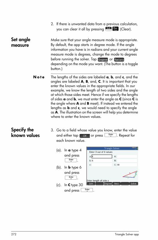
272 Triangle Solver app
2. If there is unwanted data from a previous calculation, you can clear it all by pressing SJ (Clear).
Set angle measure
Make sure that your angle measure mode is appropriate. By default, the app starts in degree mode. If the angle information you have is in radians and your current angle measure mode is degrees, change the mode to degrees before running the solver. Tap or depending on the mode you want. (The button is a toggle button.)
N o t e The lengths of the sides are labeled a, b, and c, and the angles are labeled A, B, and, C. It is important that you enter the known values in the appropriate fields. In our example, we know the length of two sides and the angle at which those sides meet. Hence if we specify the lengths of sides a and b, we must enter the angle as C (since C is the angle where A and B meet). If instead we entered the lengths as b and c, we would need to specify the angle as A. The illustration on the screen will help you determine where to enter the known values.
Specify the known values
3. Go to a field whose value you know, enter the value and either tap or press E. Repeat for each known value.
(a). In a type 4 and press E.
(b). In b type 6 and press E.
(c). In C type 30 and press E.
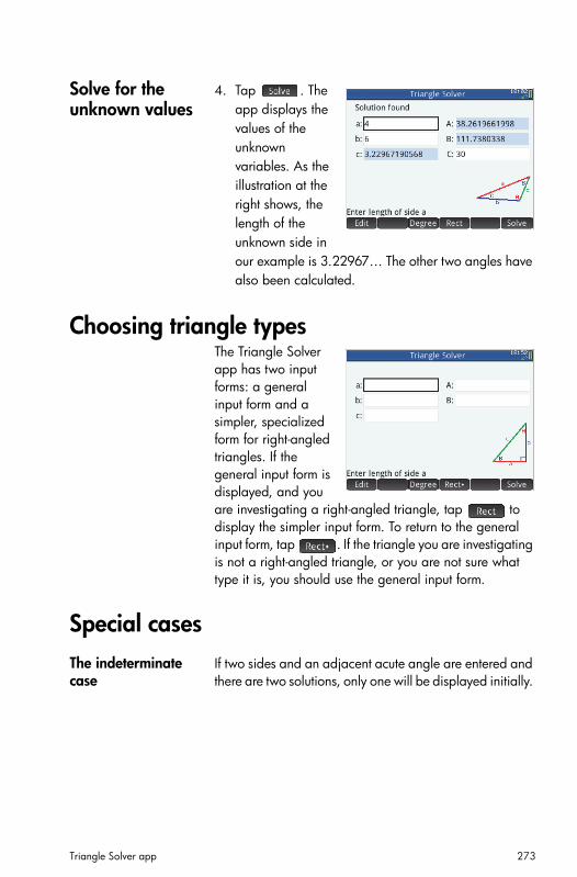
Triangle Solver app 273
Solve for the unknown values
4. Tap . The app displays the values of the unknown variables. As the illustration at the right shows, the length of the unknown side in our example is 3.22967… The other two angles have also been calculated.
Choosing triangle typesThe Triangle Solver app has two input forms: a general input form and a simpler, specialized form for right-angled triangles. If the general input form is displayed, and you are investigating a right-angled triangle, tap to display the simpler input form. To return to the general input form, tap . If the triangle you are investigating is not a right-angled triangle, or you are not sure what type it is, you should use the general input form.
Special casesThe indeterminate case
If two sides and an adjacent acute angle are entered and there are two solutions, only one will be displayed initially.
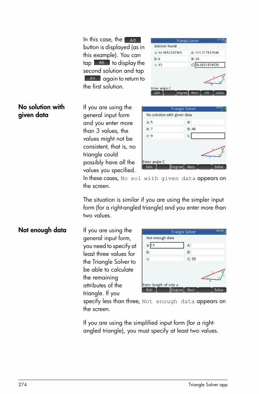
274 Triangle Solver app
In this case, the button is displayed (as in this example). You can tap to display the second solution and tap
again to return to the first solution.
No solution with given data
If you are using the general input form and you enter more than 3 values, the values might not be consistent, that is, no triangle could possibly have all the values you specified. In these cases, No sol with given data appears on the screen.
The situation is similar if you are using the simpler input form (for a right-angled triangle) and you enter more than two values.
Not enough data If you are using the general input form, you need to specify at least three values for the Triangle Solver to be able to calculate the remaining attributes of the triangle. If you specify less than three, Not enough data appears on the screen.
If you are using the simplified input form (for a right-angled triangle), you must specify at least two values.

The Explorer apps 275
19
The Explorer apps
There are three explorer apps. These are designed for you to explore the relationships between the parameters of a function and the shape of the graph of that function. The explorer apps are:
• Linear Explorer
For exploring linear functions
• Quadratic Explorer
For exploring quadratic functions
• Trig Explorer
For exploring sinusoidal functions
There are two modes of exploration: graph mode and equation mode. In graph mode you manipulate a graph and note the corresponding changes in its equation. In equation mode you manipulate an equation and note the corresponding changes in its graphical representation. Each explorer app has a number of equations and graphs for to explore, and app has a test mode. In test mode, you test you skills at matching equations to graphs.
Linear Explorer appThe Linear Explorer app can be used to explore the behavior of the graphs of and as the values of a and b change.
Open the app Press I and select Linear Explorer.
The left half of the display shows the graph of a linear function. The right half shows the general
y ax= y ax b+=

276 The Explorer apps
form of the equation being explored at the top and, below it, the current equation of that form. The keys you can use to manipulate the graph or equation appear below the equation. The x- and y-intercepts are given at the bottom.
There are two types (or levels) of linear equation available for you to explore: y = ax and y = ax + b. You choose between them by tapping or .
The keys available to you to manipulate the graph or equation depend on the level you have chosen. For example, the screen for a level 1 equation shows this:
This means that you can press <, >, +, w and Q. If you choose a level 2 equation, the screen shows this:
This means that you can press <, >, =, \, +, w and Q.
Graph mode The app opens in graph mode (indicated by the dot on the Graph button at the bottom of the screen). In graph mode, the =and \ keys translate the graph vertically, effectively changing the y-intercept of the line. Tap to change the magnitude of the increment for vertical translations. The < and > keys (as well as w and+) decrease and increase the slope. Press Q to change the sign of the slope.
The form of the linear function is shown at the top right of the display, with the current equation that matches the graph just below it. As you manipulate the graph, the equation updates to reflect the changes.

The Explorer apps 277
Equation mode Tap to enter equation mode. A dot will appear on the Eq button at the bottom of the screen.
In equation mode, you use the cursor keys to move between parameters in the equation and change their values, observing the effect on the graph displayed. Press \ or = to decrease or increase the value of the selected parameter. Press > or < to select another parameter. PressQ to change the sign of a.
Test mode Tap to enter test mode. In Test mode you test your skill at matching an equation to the graph shown. Test mode is like equation mode in that you use the cursor keys to select and change the value of each parameter in the equation. The goal is to try to match the graph that is shown.
The app displays the graph of a randomly chosen linear function of the form dictated by your choice of level. (Tap
or to change the level.) Now press the cursor keys to select a parameter and set its value. When you are ready, tap to see if you have correctly matched your equation to the given graph.
Tap to see the correct answer and tap to exit Test mode.
Quadratic Explorer appThe Quadratic Explorer app can be used to investigate the behavior of as the values of a, h and v change.
y a x h+ 2 v+=

278 The Explorer apps
Open the app PressI and select Quadratic
Explorer.
The left half of the display shows the graph of a quadratic function. The right half shows the general form of the equation being explored at the top and, below it, the current equation of that form. The keys you can use to manipulate the graph or equation appear below the equation. (These will change depending on the level of equation you choose.) Displayed beneath they keys is the equation, the discriminant (that is, ), and the roots of the quadratic.
Graph mode The app opens in graph mode. In graph mode, you manipulate a copy of the graph using whatever keys are available. The original graph—converted to dotted lines—remains in place for you to easily see the result of your manipulations.
Four general forms of quadratic equations are available for you to explore:
[Level 1]
[Level 2]
[Level 3]
[Level 4]
Choose a general form by tapping the Level button— , and so on—until the form you want is displayed. The keys available to you to manipulate the graph vary from level to level.
b2
4ac–
y ax2=
y x h+ 2=
y x2 v+=
y a x h+ 2 v+=

The Explorer apps 279
Equation mode Tap to move to equation mode. In equation mode, you use the cursor keys to move between parameters in the equation and change their values, observing the effect on the graph displayed. Press \ or = to decrease or increase the value of the selected parameter. Press > or < to select another parameter. PressQ to change the sign. You have four forms (or levels) of graph, and the keys available for manipulating the equation depend on the level chosen.
Test mode Tap to enter test mode. In Test mode you test your skill at matching an equation to the graph shown. Test mode is like equation mode in that you use the cursor keys to select and change the value of each parameter in the equation. The goal is to try to match the graph that is shown.
The app displays the graph of a randomly chosen quadratic function. Tap the Level button to choose between one of four forms of quadratic equation. You can also choose graphs that are relatively easy to match or graphs that are harder match (by tapping or
respectively).
Now press the cursor keys to select a parameter and set its value. When you are ready, tap to see if you have correctly matched your equation to the given graph.
Tap to see the correct answer and tap to exit Test mode.

280 The Explorer apps
Trig Explorer appThe Trig Explorer app can be used to investigate the behavior of the graphs and
as the values of a, b, c and d change.
The menu items available in this app are:
• or : toggles between graph mode and equation mode
• or : toggles between sine and cosine graphs
• or : toggles between radians and degrees as the angle measure for x
• or : toggles between translating the graph ( ), and changing its frequency or amplitude ( ). You make these changes using the cursor keys.
• : enters test mode
• or : toggles the increment by which parameter values change: /9, /6, /4, or 20°, 30°, 45° (depending on angle measure setting)
Open the app Press I and select Trig Explorer.
An equation is shown at the top of the display, with its graph shown below it.
Choose the type of function you want to explore by tapping either or
.
y a bx c+ sin d+=
y a bx c+ d+cos=

The Explorer apps 281
Graph mode The app opens in graph mode. In graph mode, you manipulate a copy of the graph by pressing the cursor keys. All four keys are available. The original graph—converted to dotted lines—remains in place for you to easily see the result of your manipulations.
When is chosen, the cursor keys simply translate the graph horizontally and vertically. When is chosen, pressing = or \ changes the amplitude of the graph (that is, it is stretched or shrunk vertically); and pressing < or > changes the frequency of the graph (that is, it is stretched or shrunk horizontally).
The or button at the far right of the menu determines the increment by which the graph moves with each press of a cursor key. By default, the increment is set at or 20°.
Equation mode Tap to switch to equation mode. In equation mode, you use the cursor keys to move between parameters in the equation and change their values. You can then observe the effect on the graph displayed. Press \ or = to decrease or increase the value of the selected parameter. Press > or < to select another parameter.
You can switch back to graph mode by tapping .
9
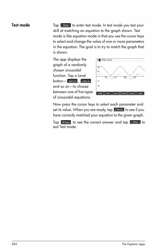
282 The Explorer apps
Test mode Tap to enter test mode. In test mode you test your skill at matching an equation to the graph shown. Test mode is like equation mode in that you use the cursor keys to select and change the value of one or more parameters in the equation. The goal is to try to match the graph that is shown.
The app displays the graph of a randomly chosen sinusoidal function. Tap a Level button— , and so on—to choose between one of five types of sinusoidal equations.
Now press the cursor keys to select each parameter and set its value. When you are ready, tap to see if you have correctly matched your equation to the given graph.
Tap to see the correct answer and tap toexit Test mode.

Functions and commands 283
20
Functions and commands
Many mathematical functions are available from the calculator’s keyboard. These are described in “Keyboard functions” on page 285. Other functions and commands are collected together in the Toolbox menus (D). There are five Toolbox menus:
• Math
A collection of non-symbolic mathematical functions (see “Keyboard functions” on page 285)
• CAS
A collection of symbolic mathematical functions (see “CAS menu” on page 298)
• App
A collection of app functions that can be called from elsewhere in the calculator, such as Home view, CAS view, the Spreadsheet app, and in a program (see “App menu” on page 312)
Note that the Geometry app functions can be called from elsewhere in the calculator, but they are not available from the App menu. For that reason, the Geometry functions are not described in this chapter, They are described in the Geometry chapter.
• User
The functions that you have created (see “Creating your own functions” on page 371) and the programs you have created that contain global
• Catlg
All the functions and commands:
– on the Math menu
– on the CAS menu
– used in the Geometry app
– used in programming

284 Functions and commands
– used in the Matrix Editor
– used in the List Editor
– and some additional functions and commands
See “Ctlg menu” on page 338.
Some functions can be chosen from the math template (displayed by pressing F). See “Math template” on page 21.
You can also create your own functions. See “Creating your own functions” on page 371.
Setting the form of menu items
You can choose to have entries on the Math and CAS menus presented either by their descriptive name or their command name. (The entries on the Catlg menu are always presented by their command name.)
The default menu presentation mode is to provide the descriptive names for the Math and CAS functions. If you prefer the functions to be presented by their command name, deselect the Menu Display option on the second page of the Home Settings screen (see “Home settings” on page 27).
Abbreviations used in this chapter
In describing the syntax of functions and commands, the following abbreviations are used:
Expr: a mathematical expression
Poly: a polynomial
LstPoly: a list of polynomials
Frac: a fraction
Descriptive name Command name
Factors List ifactors
Complex Zeros cZeros
Groebner Basis gbasis
Factor by Degree factor_xn
Find Roots proot

Functions and commands 285
RatFrac: a rational fraction
Fnc: a function
Var: a variable
LstVar: a list of variables
Keyboard functionsThe most frequently used functions are available directly from the keyboard. Many of the keyboard functions also accept complex numbers as arguments. Enter the keys and inputs shown below and press E to evaluate the expression.
In the examples below, shifted functions are represented by the actual keys to be pressed, with the function name shown in parentheses. For example, Se(ASIN) means that to make an arc sine calculation (ASIN), you press Se.
The examples below show the results you would get in Home view. If you are in the CAS, the results are given in simplified symbolic format. For example:
Sj 320 returns 17.88854382 in Home view, and 8*√5 in the CAS.
+,w,s,n
Add, subtract, multiply, divide. Also accepts complex numbers, lists, and matrices.
value1 + value2, etc.
h Natural logarithm. Also accepts complex numbers.
h(value)
Example:
h(1) returns 0
Sh (ex) Natural exponential. Also accepts complex numbers.
Shvalue
Example:
Sh5 returns 148.413159103

286 Functions and commands
i Common logarithm. Also accepts complex numbers.
i(value)
Example:
i(100) returns 2
Si (10x) Common exponential (antilogarithm). Also accepts complex numbers.
Si value
Example:
Si 3 returns 1000
efg Sine, cosine, tangent. Inputs and outputs depend on the current angle format: degrees or radians.
SIN(value)COS(value)TAN(value)
Example:
TAN(45) returns 1 (degrees mode)
Se(ASIN) Arc sine: sin–1x. Output range is from –90° to 90° or –/2 to /2. Inputs and outputs depend on the current angle format. Also accepts complex numbers.
ASIN(value)
Example:
ASIN(1) returns 90 (degrees mode)
Sf(ACOS) Arc cosine: cos–1x. Output range is from 0° to 180° or 0 to . Inputs and outputs depend on the current angle format. Also accepts complex numbers. Output will be complex for values outside the normal cosine domain of .
ACOS(value)
Example:
ACOS(1) returns 0 (degrees mode)
Sg(ATAN) Arc tangent: tan–1x. Output range is from –90° to 90° or –/2 to /2. Inputs and outputs depend on the current angle format. Also accepts complex numbers.
ATAN(value)
1– x 1

Functions and commands 287
Example:
ATAN(1) returns 45 (degrees mode)
j Square. Also accepts complex numbers.
value j
Example:
18j returns 324
Sj Square root. Also accepts complex numbers.
)Sjvalue
Example:
Sj 320 returns 17.88854382
k x raised to the power of y. Also accepts complex numbers.
value kpower
Example:
2 k8 returns 256
Sk The nth root of x.
root kvalue
Example:
3 k8 returns 2
Sn Reciprocal.
value Sn
Example:
3 Sn returns .333333333333
Q- Negation. Also accepts complex numbers.
Qvalue
Example:
Q(1+2*i) returns -1-2*i
SQ(|x|) Absolute value.

288 Functions and commands
SQ(value)SQ((x+y*i))SQ(matrix)
For a complex number, ABS((x+y*i)) returns . For a matrix, ABS returns the Frobenius norm of the matrix.
Example:
ABS(–1) returns 1ABS((1,2)) returns 2.2360679775
Math menuPress D to open the Toolbox menus (one of which is the Math menu). The functions and commands available on the Math menu are listed as they are categorized on the menu.
NumbersCeiling Smallest integer greater than or equal to value.
CEILING(value)
Examples:
CEILING(3.2) returns 4CEILING(-3.2) returns -3
Floor Greatest integer less than or equal to value.
FLOOR(value)
Example:
FLOOR(3.2) returns 3 FLOOR(-3.2) returns -4
IP Integer part.
IP(value)
Example:
IP(23.2) returns 23
x2 y2+

Functions and commands 289
FP Fractional part.
FP(value)
Example:
FP (23.2) returns .2
Round Rounds value to decimal places. Also accepts complex numbers.
ROUND(value,places)
ROUND can also round to a number of significant digits if places is a negative integer (as shown in the second example below).
Examples:
ROUND(7.8676,2) returns 7.87 ROUND(0.0036757,-3) returns 0.00368
Truncate Truncates value to decimal places. Also accepts complex numbers.
TRUNCATE(value,places)
Example:
TRUNCATE(2.3678,2) returns 2.36
Mantissa Mantissa—that is, the significant digits—of value, where value is a floating-point number.
MANT(value)
Example:
MANT(21.2E34) returns 2.12
Exponent Exponent of value. That is, the integer component of the power of 10 that generates value.
XPON(value)
Example:
XPON(123456) returns 5 (since 105.0915... equals 123456)
ArithmeticMaximum Maximum. The greater of two values.
MAX(value1,value2)
Example:

290 Functions and commands
MAX(8/3,11/4) returns 2.75
Note that in Home view a non-integer result is given as a decimal fraction. If you want to see the result as a vulgar fraction, press K. This opens the computer algebra system. If you want to return to Home view to make further calculations, press H.
Minimum Minimum. The lesser of two values.
MIN(value1,value2)
Example:
MIN(210,25) returns 25
Modulus Modulo. The remainder of value1/value2.
value1 MOD value2
Example:
74 MOD 5 returns 4
Find Root Function root-finder (like the Solve app). Finds the value for the given variable at which expression most nearly evaluates to zero. Uses guess as initial estimate.
FNROOT(expression,variable,guess)
Example:
FNROOT((A*9.8/600)-1,A,1) returns 61.224489796.
Percentage x percent of y; that is, x/100*y.
%(x,y)
Example:
%(20,50) returns 10
Complex
Argument Argument. Finds the angle defined by a complex number. Inputs and outputs use the current angle format set in Home modes.
ARG(x+y*i)
Example:
ARG(3+3*i) returns 45 (degrees mode)
Conjugate Complex conjugate. Conjugation is the negation (sign reversal) of the imaginary part of a complex number.

Functions and commands 291
CONJ(x+y*i)
Example:
CONJ(3+4*i) returns (3-4*i)
Real Part Real part x, of a complex number, (x+y*i).
RE(x+y*i)
Example:
RE(3+4*i) returns 3
Imaginary Part Imaginary part, y, of a complex number, (x+y*i).
IM(x+y*i)
Example:
IM(3+4*i) returns 4
Unit Vector Sign of value. If positive, the result is 1. If negative, –1. If zero, result is zero. For a complex number, this is the unit vector in the direction of the number.
SIGN(value)SIGN((x,y))
Examples:
SIGN(POLYEVAL[1,2,–25,–26,2],–2) returns –1SIGN((3,4)) returns (.6,.8)
Exponential
ALOG Antilogarithm (exponential).
ALOG(value)
EXPM1 Exponent minus 1: .
EXPM1(value)
LNP1 Natural log plus 1: ln(x+1).
LNP1(value)
TrigonometryThe trigonometry functions can also take complex numbers as arguments. For SIN, COS, TAN, ASIN, ACOS, and ATAN, see “Keyboard functions” on page 285.
CSC Cosecant: 1/sinx.
CSC(value)
ex 1–

292 Functions and commands
ACSC Arc cosecant.
ACSC(value)
SEC Secant: 1/cosx.
SEC(value)
ASEC Arc secant.
ASEC(value)
COT Cotangent: cosx/sinx.
COT(value)
ACOT Arc cotangent.
ACOT(value)
HyperbolicThe hyperbolic trigonometry functions can also take complex numbers as arguments.
SINH Hyperbolic sine.
SINH(value)
ASINH Inverse hyperbolic sine: sinh–1x.
ASINH(value)
COSH Hyperbolic cosine
COSH(value)
ACOSH Inverse hyperbolic cosine: cosh–1x.
ACOSH(value)
TANH Hyperbolic tangent.
TANH(value)
ATANH Inverse hyperbolic tangent: tanh–1x.
ATANH(value)
ProbabilityFactorial Factorial of a positive integer. For non-integers, ! = (x + 1).
This calculates the gamma function.
value!
Example:

Functions and commands 293
5! returns 120
Combination The number of combinations (without regard to order) of n things taken r at a time.
COMB(n,r)
Example: Suppose you want to know how many ways five things can be combined two at a time.
COMB(5,2)returns 10.
Permutation Number of permutations (with regard to order) of n things taken r at a time.
PERM (n,r)
Example: Suppose you want to know how many permutations there are for five things taken two at a time.
PERM(5,2)returns 20.
Random
Number Random number. With no argument, this function returns a random number between zero and one. With one integer argument a, it returns a random number between 0 and a. With three integer arguments, n, a, and b, returns n random number between a and b.
RANDOM
RANDOM(a)
RANDOM(n,a,b)
Integer Random integer. With one integer argument a, it returns a random integer between 0 and a. With three integer arguments, n, a, and b, returns n random integers between a and b.
RANDINT(a)
RANDINT(n,a,b)
Normal Random real number with normal distribution N(,).
RANDNORM(,)
Seed Sets the seed value on which RAND() operates. By specifying the same seed value on two or more calculators, you ensure that the same random numbers appear on each calculator when RAND() is executed.
RANDSEED(value)

294 Functions and commands
Density
Normal Normal probability density function. Computes the probability density at value x, given the mean, and standard deviation, of a normal distribution. If only one argument is supplied, it is taken as x, and the assumption is that =0 and =1.
NORMALD([,,]x)
Example:
NORMALD(0.5) and NORMALD(0,1,0.5) both return 0.352065326764.
T Student’s t probability density function. Computes the probability density of the Student's t-distribution at x, given n degrees of freedom.
STUDENT(n,x)
Example:
student(3,5.2) returns 0.00366574413491.
probability density function. Computes the probability density of the distribution at x, given n degrees of freedom.
CHISQUARE(n,x)
Example:
CHISQUARE(2,3.2) returns 0.100948258997.
F Fisher (or Fisher–Snedecor) probability density function. Computes the probability density at the value x, given numerator n and denominator d degrees of freedom.
FISHER(n,d,x)
Example:
FISHER(5,5,2) returns 0.158080231095.
Binomial Binomial probability density function. Computes the probability of k successes out of n trials, each with a probability of success of p. Returns Comb(n,k) if there is no third argument. Note that n and k are integers with .
BINOMIAL(n,k,p)
Example: Suppose you want to know the probability that just 6 heads would appear during 20 tosses of a fair coin.
BINOMIAL(20,6,0.5) returns 0.03696441652002.
2 2
2
k n
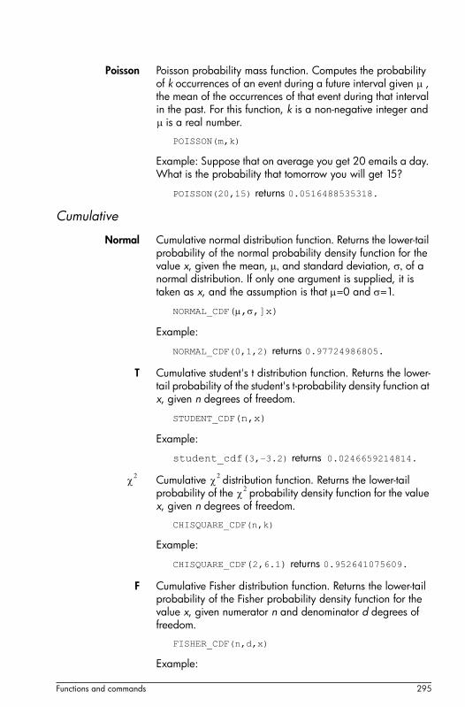
Functions and commands 295
Poisson Poisson probability mass function. Computes the probability of k occurrences of an event during a future interval given , the mean of the occurrences of that event during that interval in the past. For this function, k is a non-negative integer and
is a real number.
POISSON(m,k)
Example: Suppose that on average you get 20 emails a day. What is the probability that tomorrow you will get 15?
POISSON(20,15) returns 0.0516488535318.
Cumulative
Normal Cumulative normal distribution function. Returns the lower-tail probability of the normal probability density function for the value x, given the mean, and standard deviation, of a normal distribution. If only one argument is supplied, it is taken as x, and the assumption is that =0 and =1.
NORMAL_CDF(,,]x)
Example:
NORMAL_CDF(0,1,2) returns 0.97724986805.
T Cumulative student's t distribution function. Returns the lower-tail probability of the student's t-probability density function at x, given n degrees of freedom.
STUDENT_CDF(n,x)
Example:
student_cdf(3,–3.2) returns 0.0246659214814.
Cumulative distribution function. Returns the lower-tail probability of the probability density function for the value x, given n degrees of freedom.
CHISQUARE_CDF(n,k)
Example:
CHISQUARE_CDF(2,6.1) returns 0.952641075609.
F Cumulative Fisher distribution function. Returns the lower-tail probability of the Fisher probability density function for the value x, given numerator n and denominator d degrees of freedom.
FISHER_CDF(n,d,x)
Example:
2 2
2

296 Functions and commands
FISHER_CDF(5,5,2) returns 0.76748868087.
Binomial Cumulative binomial distribution function. Returns the probability of k or fewer successes out of n trials, with a probability of success, p for each trial. Note that n and k are integers with .
BINOMIAL_CDF(n,p,k)
Example: Suppose you want to know the probability that during 20 tosses of a fair coin you will get either 0, 1, 2, 3, 4, 5, or 6 heads.
BINOMIAL_CDF(20,0.5,6) returns 0.05765914517.
Poisson Cumulative Poisson distribution function. Returns the probability x or fewer occurrences of an event in a given time interval, given expected occurrences.
POISSON_CDF( ,x)
Example:
POISSON_CDF(4,2) returns 0.238103305554.
Inverse
Normal Inverse cumulative normal distribution function. Returns the cumulative normal distribution value associated with the lower-tail probability, p, given the mean, and standard deviation, of a normal distribution. If only one argument is supplied, it is taken as p, and the assumption is that =0 and =1.
NORMAL_ICDF([,,]p)
Example:
NORMAL_ICDF(0,1,0.841344746069) returns 1.
T Inverse cumulative student's t distribution function. Returns the value x such that the student's-t lower-tail probability of x, with n degrees of freedom, is p.
STUDENT_ICDF(n,p)
Example:
STUDENT_ICDF(3,0.0246659214814) returns –3.2.
Inverse cumulative distribution function. Returns the value x such that the lower-tail probability of x, with n degrees of freedom, is p.
k n
2 2
2

Functions and commands 297
CHISQUARE_ICDF(n,p)
Example:
CHISQUARE_ICDF(2,0.952641075609) returns 6.1.
F Inverse cumulative Fisher distribution function. Returns the value x such that the Fisher lower-tail probability of x, with numerator n and denominator d degrees of freedom, is p.
FISHER_ICDF(n,d,p)
Example:
FISHER_ICDF(5,5,0.76748868087) returns 2.
Binomial Inverse cumulative binomial distribution function. Returns the number of successes, k, out of n trials, each with a probability of p, such that the probability of k or fewer successes is q.
BINOMIAL_ICDF(n,p,q)
Example:
BINOMIAL_ICDF(20,0.5,0.6) returns 11.
Poisson Inverse cumulative Poisson distribution function. Returns the value x such that the probability of x or fewer occurrences of an event, with expected (or mean) occurrences of the event in the interval, is p.
POISSON_ICDF( ,p)
Example:
POISSON_ICDF(4,0.238103305554) returns 3.
ListThese functions work on data in a list. They are explained in detail in chapter 23, “Lists”, beginning on page 399.
MatrixThese functions work on matrix data stored in matrix . They are explained in detail in chapter 24, “Matrices”, beginning on page 411.
SpecialBeta Returns the value of the beta function ( for two reals a and b.
Beta(a,b)

298 Functions and commands
Gamma Returns the value of the gamma function ( for a number a.
Gamma(a)
Psi Returns the value of the nth derivative of the digamma function at x=a, where the digamma function is the first derivative of ln((x)).
Psi(a,n)
Zeta Returns the value of the zeta function (Z) for a real x.
Zeta(x)
erf Returns the floating point value of the error function at x=a.
erf(a)
erfc Returns the value of the complementary error function at x=a.
erfc(a)
Ei Returns the exponential integral of an expression.
Ei(Expr)
Si Returns the sine integral of an expression.
Si(Expr)
Ci Returns the cosine integral of an expression.
Ci(Expr)
CAS menuPress D to open the Toolbox menus (one of which is the CAS menu). The functions on the CAS menu are those most commonly used. Many more functions are available. See “Ctlg menu”, beginning on page 338.
Note that the Geometry functions appear on the CAS menu when the Geometry app is currently active or was the last-used app. They are described in “Geometry functions and commands”, beginning on page 151.

Functions and commands 299
AlgebraSimplify Returns an expression simplified.
simplify(Expr)
Collect Returns a polynomial or list of polynomials factorized over the field of the coefficients.
collect(Poly or LstPoly)
Expand Returns an expression expanded.
expand(Expr)
Factor Returns a polynomial factorized.
factor(Poly)
Substitute Returns the solution when a value is substituted for a variable in an expression.
subst(Expr,Var(v)=value(a))
Partial Fraction Returns the partial fraction expansion of a rational fraction.
partfrac(RatFrac)
Extract
Numerator Returns the numerator of a fraction (after simplifying the fraction if necessary).
numer(Frac(a/b) or RatFrac)
Denominator Returns the denominator of a fraction (after simplifying the fraction if necessary).
denom(Frac(a/b) or RatFrac)
Left Side Returns the left side of an equation or the left bound of an interval.
lhs(Equal(a=b) or Interval(a...b))
Right Side Returns the right side of an equation or the left bound of an interval.
rhs(Equal(a=b) or Interval(a...b))
CalculusDifferentiate With one expression as argument, returns derivative of the
expression with respect to x. With one expression and one
300 Functions and commands
variable as arguments, returns the derivative or partial derivative of the expression with respect to the variable. With one expression and more than one variable as arguments, returns the derivative of the expression with respect to the derivation in the second argument onwards. in the arguments can be followed by $k (k is an integer) to indicate the number of times the expression should be derived with respect to the variable. For example, diff(exp(x*y),x$3,y$2,z) is the same as diff(exp(x*y),x,x,x,y,y,z).
diff(Expr,[var])
or
diff(Expr,var1$k1,var2$k2,...)
Integrate Returns the indefinite integral of an expression. With one expression as argument, returns the indefinite integral with respect to x. With the optional second, third and fourth arguments you can specify the variable of integration and the bounds of the integrate.
int(Expr,[Var(x)],[Real(a)],[Real(b)])
Limit Returns the limit of an expression when the variable approaches a limit point a or +/– infinity. With the optional fourth argument you can specify whether it is the limit from below, above or bidirectional (d=–1 for limit from below and d=+1 for limit from above, d=0 for bidirectional limit). If the fourth argument is not provided, the limit returned is bidirectional.
limit(Expr,Var,Val(a),[Dir(d)])
Series Returns the series expansion of an expression in the vicinity of a given equality variable. With the optional third and fourth arguments you can specify the order and direction of the series expansion. If no order is specified the series returned is fifth order. If no direction is specified, the series is bidirectional.
series(Expr,Equal(var=limit_point),[Order],[Dir(1,0,-1)])
Summation With two arguments, returns the discrete antiderivative of the expression with respect to the variable.
sum(Expr,Var)
With four arguments, returns the discrete sum of the expression with respect to the variable from a to b.

Functions and commands 301
sum(Expr,Var,VarMin(a),VarMax(b))
Differential
Curl Returns the rotational curl of a vector field, defined by:
curl([A,B,C],[x,y,z])=[dC/dy-dB/dz,dA/dz-dC/dx,dB/dx-dA/dy].
curl(Lst(A,B,C),Lst(x,y,z))
Divergence Returns the divergence of a vector field, defined by:
divergence([A,B,C],[x,y,z])=dA/dx+dB/dy+dC/dz.
divergence(Lst(A,B,C),Lst(x,y,z))
Gradient Returns the gradient of an expression. With a list of as second argument, returns the vector of partial derivatives for all .
grad(Expr,LstVar)
Hessian Returns the Hessian matrix of an expression.
hessian(Expr,LstVar)
Integral
By Parts v(x) Performs integration by parts of the expression f(x)=u(x)*v'(x) with f(x) as the first argument and v(x) (or 0) as the second argument. With the optional third, fourth and fifth arguments you can specify a variable of integration and bounds of the integrate. If no variable of integration is provided, it is taken as x.
ibpdv(Expr(f(x)),Expr(v(x)),[Var(x)],[Real(a)],[Real(b)])
By Parts u(v) Performs integration by parts of the expression f(x)=u(x)*v'(x) with f(x) as the first argument and u(x) (or 0) as the second argument. With the optional third, fourth and fifth arguments you can specify a variable of integration and bounds of the integrate. If no variable of integration is provided, it is taken as x.
ibpu(Expr(f(x)),Expr(u(x)),[Var(x)],[Real(a)],[Real(b)])
F(b)–F(a) Returns F(b)–F(a).
preval(Expr(F(var)),Real(a),Real(b),[Var])

302 Functions and commands
Limits
Riemann Sum Returns in the neighbourhood of n=+∞ an equivalent of the sum of Xpr(var1,var2) for var2 from var2=1 to var2=var1 when the sum is looked at as a Riemann sum associated with a continuous function defined on [0,1].
sum_riemann(Expr(Xpr),Lst(var1,var2))
Taylor Returns the Taylor series expansion of an expression. With the optional second and third arguments you can specify the limit point and the order of the expansion. If no limit point is provided, it is taken as x=0. If no order is provided, the series returned is fifth order.
taylor(Expr,[Var=limit_point],[Order])
Taylor of Quotient Returns the quotient Q of the division of polynomial A by polynomial B by increasing power order, with degree(Q)≤ n or Q=0. In other words, Q is the Taylor expansion at order n of A/B in the vicinity of x=0.
divpc(A,B,Intg(n))
Transform
Laplace Returns the Laplace transform of an expression.
laplace(Expr,[Var],[LapVar])
Inverse Laplace Returns the inverse Laplace transform of an expression.
invlaplace(Expr,[Var],[IlapVar])
FFT With one argument, returns the discrete Fourier transform in R.
fft(Vect)
With three arguments, returns the discrete Fourier transform in the field Z/pZ, with a as primitive nth root of 1 (n=size(L)).
fft((Vect(L),Intg(a),Intg(p))
Inverse FFT Returns the inverse discrete Fourier transform.
ifft(Vect)
SolveSolve Returns the solutions to a polynomial equation or a set of
polynomial equations.
solve(Expr,[Var])

Functions and commands 303
Zeros With an expression as argument, returns the zeros (real or complex according to the mode) of the expression. With a list of expressions as argument, returns the matrix where the lines are the solutions of the system (i.e. expression1=0, expression2=0,...,).
zeros(Expr,[Var])
or
zeros([LstExpr],[LStVar])
Complex Solve Returns a list where the elements are complex solutions of the system of polynomial equations.
csolve(LstEq,LstVar)
Complex Zeros With an expression as argument, returns the complex zeros of the expression. With a list of expressions as argument, returns the matrix where the lines are the solutions of the system (i.e. expression1=0, expression2=0,...,).
Czeros(Expr,[Var])
or
Czeros([LstExpr],[LStVar])
Numerical Solve Returns the numerical solution of an equation or a system of equations. With the optional third argument you can specify a guess for the solution or an interval within which it is expected that the solution will occur. With the optional fourth argument you can name the iterative algorithm to be used by the solver.
nSolve(Expr,Var,[Guess or Interval],[Method])
DifferentialEquation
Returns the solution to a differential equation.
deSolve(Eq,[TimeVar],FncVar)
ODE Solve Returns an approximate value of y at a final value (t1) of a given variable, where y(t) is the solution of: y’(t)=f(t,y(t)), y(t0)=y0.
odesolve(Expr(f(t,y)),VectVar([t,y]),VectInitCond([t0,y0]),FinalVal(t1),[tstep=Val,curve])
Linear System Returns the solution to a system of linear equations.
linsolve(LstLinEq,LstVar)

304 Functions and commands
Rewritelncollect Returns an expression rewritten with the logarithms collected.
(applies ln(a)+n*ln(b)->ln(a*b^n) for integers n).
lncollect(Expr)
powexpand Returns an expression with a power of sum rewritten as a product of powers.
powexpand(Expr)
tExpand Returns a transcendental expression in expanded form.
tExpand(Expr)
Exp & Ln
ey*lnx Returns an expression of the form exp(n*ln(x)) rewritten as a power of x.
exp2pow(Expr)
y*lnx Returns an expression with powers rewritten as an exponentials.
pow2exp(Expr)
exp2trig Returns an expression with complex exponentials rewritten in terms of sin and cos.
exp2trig(Expr)
expexpand Returns an expression with exponentials in expanded form.
expexpand(Expr)
Sine
asinx → acosx Returns an expression with arcsin(x) rewritten as pi/2-arccos(x).
asin2acos(Expr)
asinx → atanx Returns an expression with arcsin(x) rewritten as arctan(x/sqrt(1-x^2)).
asin2atan(Expr)
sinx → cosx/tanx Returns an expression with sin(x) rewritten as cos(x)*tan(x).
sin2costan(Expr)

Functions and commands 305
Cosine
acosx → asinx Returns an expression with arccos(x) rewritten as pi/2-arcsin(x).
acos2asin(Expr)
acosx → atanx Returns an expression with arccos(x) rewritten as pi/2-arctan(x/sqrt(1-x^2)).
acos2atan(Expr)
cosx → sinx/tanx Returns an expression with cos(x) rewritten as sin(x)/tan(x).
cos2sintan(Expr)
Tangent
atanx → asinx Returns an expression with arctan(x) rewritten as arcsin(x/sqrt(1+x^2)).
atan2asin(Expr)
atanx → acosx Returns an expression with arctan(x) rewritten as pi/2-arccos(x/sqrt(1+x^2)).
atan2acos(Expr)
tanx → sinx/cosx Returns an expression with tan(x) rewritten as sin(x)/cos(x).
tan2sincos(Expr)
halftan Returns an expression with sin(x), cos(x) or tan(x) rewritten as tan(x/2).
halftan(Expr)
Trig
trigx → sinx Returns an expression simplified using the formulas sin(x)^2+cos(x)^2=1 and tan(x)=sin(x)/cos(x) (privileging sine).
trigsin(Expr)
trigx → cosx Returns an expression simplified using the formulas sin(x)^2+cos(x)^2=1 and tan(x)=sin(x)/cos(x) (privileging cosine).
trigcos(Expr)
trigx → tanx Returns an expression simplified using the formulas sin(x)^2+cos(x)^2=1 and tan(x)=sin(x)/cos(x) (privileging tangent).

306 Functions and commands
trigtan(Expr)
atrig2ln Returns an expression with inverse trigonometric functions rewritten as logarithmic functions.
atrig2ln(Expr)
tlin Returns a trigonometric expression with the products and integer powers linearized.
tlin(ExprTrig)
tCollect Returns a trigonometric expression linearized and with any sine and cosine of the same angle put together.
tCollect(Expr)
trigexpand Returns a trigonometric expression in expanded form.
trigexpand(Expr)
trig2exp Returns an expression with trigonometric functions rewritten as complex exponentials (without linearization).
trig2exp(Expr)
IntegerDivisors Returns the list of divisors of an integer or a list of integers.
idivis(Intg(a) or (LstIntg))
Factors Returns an integer decomposed into its prime factors.
ifactor(Intg(a))
Factor List Returns the list of prime factors of an integer or a list of integers. Each factor is followed by its multiplicity.
ifactors(Intg(a) or (LstIntg))
GCD Returns the greatest common divisor of two integers.
gcd((Intg(a),Intg(b))
LCM Returns the lowest common multiple of two integers.
lcm((Intg(a),Intg(b))
Prime
Test if Prime Tests whether or not a given integer is a prime number.
isprime(Intg(a))

Functions and commands 307
Nth Prime Returns the nth prime number less than 10000.
ithprime(Intg(n))
Next Prime Returns the next prime or pseudo-prime after an integer.
nextprime(Intg(a))
Previous Prime Returns the prime or pseudo-prime number closest to but smaller than an integer.
prevprime(Intg(a))
Euler Compute’s Euler's totient for an integer.
euler(Intg(n))
Division
Quotient Returns the integer quotient of the Euclidean division of two integers.
iquo(Intg(a),Intg(b))
Remainder Returns the integer remainder from the Euclidean division of two integers.
irem(Intg(a),Intg(b))
an MOD p Returns an modulo p in [0;p−1].
powmod(Intg(a),Intg(n),Intg(p),[Expr(P(x))],[Var])
ChineseRemainder
Returns the Chinese remainder of two lists of integers.
ichinrem(LstIntg(a,p),LstIntg(b,q))
PolynomialFind Roots Returns all computed roots of a polynomial given by its
coefficients. (It may not work if roots are not simple.)
proot(Vect||Poly)
Coefficients With an integer as third argument, returns the coefficient of a polynomial of degree given in the third argument. With no third argument, returns the list of coefficients of the polynomial.
coeff(Expr,[Var],degree)
Divisors Returns the list of divisors of a polynomial or a list of polynomials.

308 Functions and commands
divis(Poly or LstPoly)
Factor List Returns the list of prime factors of a polynomial or a list of polynomials. Each factor is followed by its multiplicity.
factors(Poly or LstPoly)
GCD Returns the greatest common divisor of two polynomials of several .
gcd(Poly,Poly)
LCM Returns the lowest common multiple of two polynomials of several .
lcm(Poly,Poly))
Create
Poly to Coef With a variable as second argument, returns the coefficients of a polynomial with respect to the variable. With a list of as second argument, returns the internal format of the polynomial.
symb2poly(Expr,[Var])
or
symb2poly(Expr,ListVar)
Coef to Poly With one list as argument, returns a polynomial in x with coefficients (in decreasing order) obtained from the list. With a variable as second argument, returns a polynomial in the variable as for one argument but the polynomial is in the variable specified in the second argument.
poly2symb(Lst,Var)
Roots to Coef Returns the coefficients (in decreasing order) of the univariate polynomial of roots specified in the argument.
pcoef(Vect)
Roots to Poly Returns the rational function that has the roots and poles specified in the argument.
fcoeff(Lst(root||pole,order))
Random Returns a polynomial of variable specified in the first argument, of degree n and where the coefficients are random integers in the range −99 through 99 with uniform distribution or according to the law specified in the third argument.
randPoly([Var(var)],Intg(n),[law])

Functions and commands 309
Minimum With only a matrix as argument, returns the minimal polynomial in x of a matrix written as a list of its coefficients. With a matrix and a variable as arguments, returns the minimum polynomial of the matrix written in symbolic form with respect to the variable.
pmin(Mtrx,[Var])
Algebra
Quotient Returns the Euclidean quotient of two polynomials written as vectors or in symbolic form.
quo((Vect),(Vect),[Var])
or
quo((Poly),(Poly),[Var])
Remainder Returns the Euclidean remainder of two polynomials written as vectors or in symbolic form.
rem((Vect),(Vect),[Var])
or
rem((Poly),(Poly),[Var])
Degree Returns the degree of a polynomial.
degree(Poly)
Factor by Degree Returns a polynomial factorized in x^n, where n is the degree of polynomial.
factor_xn(Poly)
Coef. of GCD Returns the greatest common divisor (GCD) of the coefficients of a polynomial.
content(Poly(P),[Var])
Zero Count With a polynomial and a variable as arguments, returns the list of the Sturm sequences and multiplicities of the square-free factors of the polynomial with respect to the variable. With a polynomial, a variable and two reals as arguments, returns the number of sign changes of the polynomial over the interval specified by the two reals.
sturmseq(Poly,[Var])
or
sturmseq(Poly,[Var],a,b)

310 Functions and commands
ChineseRemainder
Returns the Chinese remainder of the polynomials written as lists of coefficients or in symbolic form.
chinrem([Lst||Expr,Lst||Expr],[Lst||Expr,Lst||Expr])
Special
Cyclotomic Returns the list of coefficients of the cyclotomic polynomial of an integer.
cyclotomic(Int)
Groebner Basis Returns the Groebner basis of the ideal spanned by a list of polynomials.
gbasis(LstPoly,LstVar)
GroebnerRemainder
Returns the remainder of the division of a polynomial by the Groebner basis of a list of polynomials.
greduce(Poly,LstPoly,LstVar)
Hermite Returns the Hermite polynomial of degree n.
hermite(Intg(n))
Lagrange Returns the Lagrange polynomial for two lists. The list in the first argument corresponds to the abscissa values, and the list in the second argument corresponds to the ordinate values.
lagrange((Lst_xk,Lst_yk)
or
lagrange(Mtrx_2*n)
Laguerre Returns the Laguerre polynomial of degree n.
laguerre(Intg(n))
Legendre Returns the Legendre polynomial of degree n.
legendre(Intg(n))
Chebyshev Tn Returns the Tchebyshev polynomial of first kind of degree n.
tchebyshev1(Intg(n))
Chebyshev Un Returns the Tchebyshev polynomial of second kind of degree n.
tchebyshev2(Intg(n))

Functions and commands 311
PlotFunction Plots the graph of an expression of one or two with
superposition.
plotfunc(Expr,[Var(x)],[Intg(color)])
or
plotfunc(Expr,[VectVar],[Intg(color)])
Implicit Plots the graph of the implicit equation f(Var1,Var2)=0.
plotimplicit(Expr,Var1,Var2)
Density Plots the graph of the function z=f(x,y) in the plane where the values of z are represented by different colors.
plotdensity(Expr,[x=xrange,y=yrange],[z],[xstep],[ystep])
Slopefield Draws the tangent of the differential equation y'=f(t,y), where the first argument is the expression f(t,y) (y is the real variable and t is the abscissa), the second argument is the vector of (abscissa must be listed first), and the third argument is the optional range.
plotfield(Expr,VectVar,[Opt])
Contour Draws eleven contour lines of the surface defined by the expression z=f(x,y) for z=−10,−8,...,8,10. With a list of values as third argument, contour lines will be drawn instead for the z values given in the list.
plotcontour(Expr(Xpr),[LstVar],[LstVal])
ODE Draws the solution of the differential equation y'=f(t,y) that crosses the point (t0,y0), where the first argument is the expression f(t,y), the second argument is the vector of (abscissa must be listed first), and the third argument is (t0,y0).
plotode(Expr,VectVar,VectInitCond)
List Draws the polygonal line through the points of abscissa 0,...,n and ordinate l=[y0,...,yn], or draws the line through the points of abscissa (the first column in the matrix) and ordinate (the second column in the matrix).
plotlist(Lst(l)||Mtrx(M))

312 Functions and commands
App menuPress D to open the Toolbox menus (one of which is the App menu). App functions are used in HP apps to perform common calculations. For example, in the Function app, the Plot view Fcn menu has a function called SLOPE that calculates the slope of a given function at a given point. The SLOPE function can also be used from the Home view or a program to give the same results The App functions described in this section are grouped by app.
Function app functionsThe Function app functions provide the same functionality found in the Function app's Plot view under the FCN menu. All these operations work on functions. The functions may be expressions in X or the names of the Function app variable F0 through F9.
AREA Area under a curve or between curves. Finds the signed area under a function or between two functions. Finds the area under the function Fn or below Fn and above the function Fm, from lower X-value to upper X-value.
AREA(Fn,[Fm,]lower,upper)
Example:
AREA(-X,X2-2,-2,1) returns 4.5
EXTREMUM Extremum of a function. Finds the extremum (if one exists) of the function Fn that is closest to the X-value guess.
EXTREMUM(Fn, guess)
Example:
EXTREMUM(X2-X-2,0) returns 0.5
ISECT Intersection of two functions. Finds the intersection (if one exists) of the two functions Fn and Fm that is closest to the X-value guess.

Functions and commands 313
ISECT(Fn,Fm,guess)
Example:
ISECT(X,3-X,2) returns 1.5
ROOT Root of a function. Finds the root of the function Fn (if one exists) that is closest to the X-value guess.
ROOT(Fn,guess)
Example:
ROOT(3-X2,2) returns 1.732…
SLOPE Slope of a function. Returns the slope of the function Fn at the X-value (if value exists).
SLOPE(Fn,value)
Example:
SLOPE(3-X2,2) returns -4
Solve app functionsThe Solve app has a single function that solves a given equation or expression for one of its . En may be an equation or expression, or it may be the name of one of the Solve Symbolic E0-E9.
SOLVE Solve. Solves an equation for one of its . Solves the equation En for the variable var, using the value of guess as the initial value for the value of the variable var. If En is an expression, then the value of the variable var that makes the expression equal to zero is returned.
SOLVE(En,var,guess)
Example:
SOLVE(X2-X-2,X,3)returns 2
This function also returns an integer that is indicative of the type of solution found, as follows:
0—an exact solution was found
1—an approximate solution was found
2—an extremum was found that is as close to a solution as possible
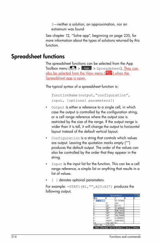
314 Functions and commands
3—neither a solution, an approximation, nor an extremum was found
See chapter 12, “Solve app”, beginning on page 235, for more information about the types of solutions returned by this function.
Spreadsheet functionsThe spreadsheet functions can be selected from the App Toolbox menu (D > > Spreadsheet). They can also be selected from the View menu (V) when the Spreadsheet app is open.
The typical syntax of a spreadsheet function is:
functionName(output,“configuration”,
input, [optional parameters])
• Output is either a reference to a single cell, in which case the output is controlled by the configuration string, or a cell range reference where the output size is restricted by the size of the range. If the output range is wider than it is tall, it will change the output to horizontal layout instead of the default vertical layout.
• Configuration is a string that controls which values are output. Leaving the quotation marks empty (“”) produces the default output. The order of the values can also be controlled by the order that they appear in the string.
• Input is the input list for the function. This can be a cell range reference, a simple list or anything that results in a list of values.
• [ ] denotes optional parameters.
For example: =STAT1(B1,””,A25:A37) produces the following output.
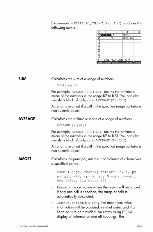
Functions and commands 315
For example: =STAT1(B1,”H ”,A25:A37) produces the following output.
SUM Calculates the sum of a range of numbers.
SUM([input])
For example, AVERAGE)B7:B23) returns the arithmetic mean of the numbers in the range B7 to B23. You can also specify a block of cells, as in AVERAGE(B7:C23).
An error is returned if a cell in the specified range contains a non-numeric object.
AVERAGE Calculates the arithmetic mean of a range of numbers.
AVERAGE([input])
For example, AVERAGE)B7:B23) returns the arithmetic mean of the numbers in the range B7 to B23. You can also specify a block of cells, as in AVERAGE)B7:C23).
An error is returned if a cell in the specified range contains a non-numeric object.
AMORT Calculates the principal, interest, and balance of a loan over a specified period.
AMORT(Range, "configuration", n, i, pv, pmt[ppyr=12, cpyr=ppyr, Grouping=ppyr, beg=false, fix=current])
• Range is the cell range where the results will be placed. If only one cell is specified, the range of cells is automatically calculated.
• Configuration is a string that determines what information will be provided, in what order, and if a heading is to be provided. An empty string ("") will display all information and all headings. The
x

316 Functions and commands
configuration codes are listed below. Add H as a prefix to have a heading generated for that information.
h – This column contains the row headers S – This column contains the start of the period E – This column contains the end of the period HB,HIP – This column contains the Principal paid this period B – This column contains the balance at the end of the period I – This column contains the interest paid this period
n is the number of periods for the loan, i is interest ratepv is the present valuepmt is the per-period payment
• Optional parameters:
ppyr is the number of payments per year
cpyr is the number of compounding periods per year
• Grouping is the number of periods that need to be grouped together in the amortization table.
beg is 1 when payment is at the beginning of each period, else it is 0. fix is the number of decimal places to be used for the calculations.
Example: =AMORT(A1,””,12,6,100,200)
STAT1 he STAT1 function provides a range of one-variable statistics. It can calculate all or any of , Σ, Σ², s, s², σ, σ², serr, sqd, n, min, q1, med, q3, and max.
STAT1(output,"configuration",input, [mode])
• Output is the cell range where the results are placed. If only one cell is specified, then the range of cells is automatically calculated.
• Configuration is a string that defines if a header row needs to be created (starts with H) and what result to place in which column. An empty string "" will use all the headers.
x
Functions and commands 317
Note that many of the characters representing statistics—for example, x
_and —can be selected from
the symbol palette (S9).
• Input is the can be a cell range reference, a simple list or anything that results in a list of values.
• Mode is optional and defines what to calculate the mean of. The valid values are:
1 = one value 2 = with frequency data 3 = with weighted data
4 = multiplies two data sets together to form a single data set
Examples:
STAT1(B1,””,A25:A37)
STAT1(B1,”Hx_,H”,A25:A37)
REGRS Regression analysis function. Can calculate all or any of sl = (slope), int (intercept), cor, cd, sCov, pCov, px (predict x), and py (predict y).
REGRS(output, "configuration", input,[mode],[y],[x])
• Output is a reference to where you would like the output to be placed. Note, if a range is specified, it will limit the size of the output, but can also change the orientation from vertical to horizontal if the range is wider than it is tall.
• Configuration is a string that controls what results are shown and in what order they appear. An empty string "" will default to show all in default order including headers.
• Input can be a cell range reference, a simple list or anything that results in a list of values.
• Input Parameters:
mode (optional) specifies the mode to be used for the regression:
1 linear2 logarithmic

318 Functions and commands
3 exponential4 power5 inverse6 logistic7 quadratic8 cubic9 quartic10 trigonometric
Important: If px or py are specified, their opposite value must be one of the input values. For example, if px is specified in the configuration string then the y-value must be an input parameter and vice versa for py.
Example: REGRS(J1,””,A25:B37,2)
PredY
PredX
HypZ1mean The hypothesis test HypZ1mean is a one-sample Z-test for comparing means.
Syntax:
HypZ1mean(ouput, "configuration",input list)
HypZ1mean(ouput, "configuration", SampMean, SampSize, NullPopMean, PopStdDev, SigLevel, Mode)
• Output is a reference to where you would like the output to be placed. Note if a range is specified it will limit the size of the output, but can also change the orientation from vertical to horizontal if the range is wider than it is tall.
• Configuration is a string that controls what results are shown and what order they appear in. An empty string "" will default to show all in default order including headers.
h = if present the header cells will be created acc = Accept/Reject

Functions and commands 319
tZ = Test Z tM = Test Meanprob = Probability cZ = Critical Z cx1 = Critical xbar 1 cx2 = Critical xbar 2 std = Standard deviation
• Input list is the list of input (see Input Parameters below). This can be a range reference, a list of cell references or a simple list of values.
• Input Parameters:
SampMean: SampSize: NullPopMean: PopStdDev: SigLevel: Mode: Specifies how to calculate the statistic
1 = Less than 2 = Greater than 3 = Not Equal
Example: XXXXX
HYPZ2mean The hypothesis test HypZ2mean is a two-sample Z-test for comparing means.
Syntax:
HypZ2mean(ouput, "configuration", input list)
HypZ2mean(ouput, "configuration", SampMean, SampMean2, SampSize,SampSize2, PopStdDev, PopStdDev2,SigLevel, Mode)
• Output is a reference to where you would like the output to be placed. Note if a range is specified it will limit the size of the output, but can also change the orientation from vertical to horizontal if the range is wider than it is tall.
• Configuration is a string that controls what results are shown and what order they appear in. An empty string

320 Functions and commands
"" will default to show all in default order including headers.
h = if present the header cells will be created acc = Accept/Reject tZ = Test Z tM = Test Mean prob = Probability cZ = Critical Z cx1 = Critical xbar 1 cx2 = Critical xbar 2 std = Standard deviation
• Input list is the list of input (see Input Parameters below). This can be a range reference, a list of cell references or a simple list of values.
• Input Parameters:
SampMean: SampMean2: SampSize: SampSize2: PopStdDev: PopStdDev2: SigLevel: Mode: Specifies how to calculate the statistic
1 = Less than2 = Greater than 3 = Not Equal
Example: XXXXX
HypZ1prop The hypothesis test HypZ1prop is a one-proportion Z-test.
Syntax:
HypZ1prop(output, "configuration", input list) HypZ1prop(ouput, "configuration", SuccCount, SampSize, NullPopProp, SigLevel, Mode)
• Output is a reference to where you would like the output to be placed. Note if a range is specified it will limit the size of the output, but can also change the orientation

Functions and commands 321
from vertical to horizontal if the range is wider than it is tall.
• Configuration is a string that controls what results are shown and what order they appear in. An empty string "" will default to show all in default order including headers.
h = if present the header cells will be created acc = Accept/Reject tZ = Test Z tP prob cZcp1 cp2 std
• Input list is the list of input (see Input Parameters below). This can be a range reference, a list of cell references or a simple list of values.
• Input Parameters:
SuccCount: SampSize: NullPopMean: SigLevel: Mode: Specifies how to calculate the statistic
1 = Less than 2 = Greater than 3 = Not Equal
Example: XXXXX
HypZ2prop The hypothesis test HypZ2prop is a two-proportion Z-test for comparing means.
Syntax:
HypZ2prop(ouput, "configuration", input list)
HypZ2prop(ouput, "configuration", SuccCount1, SuccCount2, SampSize1, SampSize2, SigLevel, Mode)

322 Functions and commands
• Output is a reference to where you would like the output to be placed. Note if a range is specified it will limit the size of the output, but can also change the orientation from vertical to horizontal if the range is wider than it is tall.
• Configuration is a string that controls what results are shown and what order they appear in. An empty string "" will default to show all in default order including headers.
h = if present the header cells will be created acc = Accept/Reject tZ = Test Z tPd prob cZ cp1 cp2 std
• Input list is the list of input (see Input Parameters below). This can be a range reference, a list of cell references or a simple list of values.
• Input Parameters:
SuccCount1 SuccCount2 SampSize1 SampSize2 SigLevel Mode: Specifies how to calculate the statistic
1 = Less than 2 = Greater than 3 = Not Equal
Example: XXXXX
HypT1mean The hypothesis test HypT1mean is a one-sample T-test for comparing means.
Syntax:
HypT1mean(ouput, "configuration", input list)

Functions and commands 323
HypT1mean(ouput, "configuration", SampMean, SampStdDev, SampSize, NullPopProp, SigLevel, Mode)
• Output is a reference to where you would like the output to be placed. Note if a range is specified it will limit the size of the output, but can also change the orientation from vertical to horizontal if the range is wider than it is tall.
• Configuration is a string that controls what results are shown and what order they appear in. An empty string "" will default to show all in default order including headers.
h = if present the header cells will be created acc = Accept/Reject tT tM prob df ct cX1 cX2
• Input list is the list of input (see Input Parameters below). This can be a range reference, a list of cell references or a simple list of values.
• Input Parameters:
SampMean SampStdDev SampSize: NullPopMean: SigLevel: Mode: Specifies how to calculate the statistic
1 = Less than2 = Greater than 3 = Not Equal
Example: XXXXX
HypT2mean The hypothesis test HypT2mean is a two-sample T-test for comparing means.

324 Functions and commands
Syntax:
HypT2mean(ouput, "configuration", input list)
HypT2mean(ouput, "configuration", SampMean1, SampMean2,SampStdDev1, SampStdDev2,SampSize1, SampSize2, pooled, SigLevel, Mode)
• Output is a reference to where you would like the output to be placed. Note if a range is specified it will limit the size of the output, but can also change the orientation from vertical to horizontal if the range is wider than it is tall.
• Configuration is a string that controls what results are shown and what order they appear in. An empty string "" will default to show all in default order including headers.
h = if present the header cells will be created acc = Accept/Reject tT tM prob df ct cX1 cX2 stD
• Input list is the list of input (see Input Parameters below). This can be a range reference, a list of cell references or a simple list of values.
• Input Parameters:
SampMean1 SampMean2 SampStdDev1 SampStdDev2 SampSize1 SampSize2 pooled = 0 == false or 1 == true

Functions and commands 325
SigLevel: Mode: Specifies how to calculate the statistic
1 = Less than 2 = Greater than 3 = Not Equal
Example: XXXXX
ConfZ1mean The ConfZ1mean calculates the confidence interval for a one-sample Z-test.
Syntax:
ConfZ1mean(ouput, "configuration", input list)
ConfZ1mean(ouput, "configuration", SampMean, SampSize, PopStdDevm ConfLevel)
• Output is a reference to where you would like the output to be placed. Note if a range is specified it will limit the size of the output, but can also change the orientation from vertical to horizontal if the range is wider than it is tall.
• Configuration is a string that controls what results are shown and what order they appear in. An empty string "" will default to show all in default order including headers.
h = if present the header cells will be created Z zXl zXh std
• Input list is the list of input (see Input Parameters below). This can be a range reference, a list of cell references or a simple list of values.
• Input Parameters: SampMean, SampSize, PopStdDevm ConfLevel
Example: XXXXX

326 Functions and commands
ConfZ2mean The ConfZ2mean calculates the confidence interval for a two-sample Z-test.
Syntax:
ConfZ2mean(ouput, "configuration", input list)
ConfZ2mean(ouput, "configuration", SampMean1, SampMean2, SampSize1, SampSize2, PopStdDev1,PopStdDev2 ConfLevel)
• Output is a reference to where you would like the output to be placed. Note if a range is specified it will limit the size of the output, but can also change the orientation from vertical to horizontal if the range is wider than it is tall.
• Configuration is a string that controls what results are shown and what order they appear in. An empty string "" will default to show all in default order including headers.
h = if present the header cells will be created Z zXl zXh zXm std
• Input list is the list of input (see Input Parameters below). This can be a range reference, a list of cell references or a simple list of values.
• Input Parameters:
SampMean1, SampMean2, SampSize1, SampSize2, PopStdDev1, PopStdDev2, ConfLevel
Example: XXXXX

Functions and commands 327
ConfZ1prop The ConfZ1prop calculates the confidence interval for a one-proportion Z-test.
Syntax:
ConfZ1prop(ouput, "configuration", input list) ConfZ1prop(ouput, "configuration", SuccCount, SampSize, ConfLevel)
• Output is a reference to where you would like the output to be placed. Note if a range is specified it will limit the size of the output, but can also change the orientation from vertical to horizontal if the range is wider than it is tall.
• Configuration is a string that controls what results are shown and what order they appear in. An empty string "" will default to show all in default order including headers.
h = if present the header cells will be created Z zXl zXh zXm std
• Input list is the list of input (see Input Parameters below). This can be a range reference, a list of cell references or a simple list of values.
• Input Parameters:
SuccCount, SampSize, ConfLevel
Example: XXXXX
ConfZ2prop The ConfZ1mean calculates the confidence interval for a two-proportion Z-test.
Syntax:
ConfZ2prop(ouput, "configuration", input list)
328 Functions and commands
ConfZ2prop(ouput, "configuration", SuccCount1, SuccCount2, SampSize1, SampSize2,ConfLevel)
• Output is a reference to where you would like the output to be placed. Note if a range is specified it will limit the size of the output, but can also change the orientation from vertical to horizontal if the range is wider than it is tall.
• Configuration is a string that controls what results are shown and what order they appear in. An empty string "" will default to show all in default order including headers.
h = if present the header cells will be created Z zXl zXh zXm std
• Input list is the list of input (see Input Parameters below). This can be a range reference, a list of cell references or a simple list of values.
• Input Parameters:
SuccCount1, SuccCount2, SampSize1, SampSize2, ConfLevel
Example: XXXXX
ConfT1mean The ConfT1mean calculates the confidence interval for a one-sample T-test.
Syntax:
ConfT1mean(ouput, "configuration", input list)
ConfT1mean(ouput, "configuration", SampMean, SampStdDev, SampSize, ConfLevel)

Functions and commands 329
• Output is a reference to where you would like the output to be placed. Note if a range is specified it will limit the size of the output, but can also change the orientation from vertical to horizontal if the range is wider than it is tall.
• Configuration is a string that controls what results are shown and what order they appear in. An empty string "" will default to show all in default order including headers.
h = if present the header cells will be created DF T zX; zXh std
• Input list is the list of input (see Input Parameters below). This can be a range reference, a list of cell references or a simple list of values.
• Input Parameters:
SampMean, SampStdDev, SampSize, ConfLevel
Example: XXXXX
ConfT2mean The ConfT2mean calculates the confidence interval for a two-sample T-test.
Syntax:
ConfT2mean(ouput, "configuration", input list)
ConfT2mean(ouput, "configuration", SampMean, SampMean2, SampStdDev, SampStdDev2, SampSize, SampSize2, pooled, ConfLevel)
• Output is a reference to where you would like the output to be placed. Note if a range is specified it will limit the size of the output, but can also change the orientation

330 Functions and commands
from vertical to horizontal if the range is wider than it is tall.
• Configuration is a string that controls what results are shown and what order they appear in. An empty string "" will default to show all in default order including headers.
h = if present the header cells will be created DF T zX; zXh zXm Std
• Input list is the list of input (see Input Parameters below). This can be a range reference, a list of cell references or a simple list of values.
• Input Parameters:
SampMean, SampMean2, SampStdDev, SampStdDev2, SampSize, SampSize2, pooled, ConfLevel
Statistics 1Var app functionsThe Statistics 1Var app has three functions designed to work together to calculate summary statistics based on one of the statistical analyses (H1-H5) defined in the Symbolic view of the Statistics 1Var app.
Do1VStats Do1:variable statistics. Performs the same calculations as tapping in the Numeric view of the Statistics 1Var app and stores the results in the appropriate Statistics 1Var app results . Hn must be one of the Statistics 1Var app Symbolic view H1-H5.
Do1VStats(Hn)
Functions and commands 331
SetFreq Set frequency. Sets the frequency for one of the statistical analyses (H1-H5) defined in the Symbolic view of the Statistics 1Var app. The frequency can be either one of the column D0-D9, or any positive integer. Hn must be one of the Statistics 1Var app Symbolic view H1-H5. If used, Dn must be one of the column D0-D9; otherwise, value must be a positive integer.
SETFREQ(Hn,Dn)
or
SETFREQ(Hn,value)
SetSample Set sample data. Sets the sample data for one of the statistical analyses (H1-H5) defined in the Symbolic view of the Statistics 1Var app. Sets the data column to one of the column D0-D9 for one of the statistical analyses H1-H5.
SETSAMPLE(Hn,Dn)
Statistics 2Var app functionsThe Statistics 2Var app has a number of functions. Some are designed to calculate summary statistics based on one of the statistical analyses (S1-S5) defined in the Symbolic view of the Statistics 2Var app. Others predict X- and Y-values based on the fit specified in one of the analyses.
PredX Predict X. Uses the fit from the first active analysis (S1-S5) found to predict an x-value given the y-value.
PredX(value)
PredY Predict Y. Uses the fit from the first active analysis (S1-S5) found to predict a y-value given the x-value.
PredY(value)
Resid Residuals. Calculates a list of residuals, based on column data and a fit defined in the Symbolic view via S1-S5.
Resid(Sn) or Resid()
Resid() looks for the first defined analysis in the Symbolic view (S1-S5).
Do2VStats Do 2:variable statistics. Performs the same calculations as tapping in the Numeric view of the Statistics 2Var app
332 Functions and commands
and stores the results in the appropriate Statistics 2Var app results . Sn must be one of the Statistics 2Var app Symbolic view S1-S5.
Do2VStats(Sn)
SetDepend Set dependent column. Sets the dependent column for one of the statistical analyses S1-S5 to one of the column C0-C9.
SetDepend(Sn,Cn)
SetIndep Set independent column. Sets the independent column for one of the statistical analyses S1-S5 to one of the column C0-C9.
SetIndep(Sn,Cn)
Inference app functionsThe Inference app has a single function that returns the same results as tapping in the Numeric view of the Inference app. The results depend on the contents of the Inference app Method, Type, and AltHyp.
DoInference Calculate confidence interval or test hypothesis. Performs the same calculations as tapping in the Numeric view of the Inference app and stores the results in the appropriate Inference app results.
DoInference()

Functions and commands 333
HypZ1mean
HypZ2mean
HypZ1prop
HypZ2prop
HypT1mean
HypT2mean
ConfZ1mean
ConfZ2mean
ConfZ1Prop
ConfZ2Prop
ConfT1mean
ConfT2mean
Finance app functionsThe Finance App uses a set of functions that all reference the same set of Finance app . There are 5 main TVM , 4 of which are mandatory for each of these functions (except DoFinance). There are 3 other that are optional and have default values. These occur as arguments to the Finance app functions in the following set order:
– NbPmt—the number of payments
– IPYR—the annual interest rate
– PV—the present value of the investment or loan
– PMTV—the payment value
– FV—the future value of the investment or loan
– PPYR—the number of payments per year (12 by default)
334 Functions and commands
– CPYR—the number of compounding periods per year (12 by default)
– END—payments made at the end of the period
The arguments PPYR, CPYR, and END are optional; if not supplied, PPYR=12, CPYR=PPYR, and END=1.
CalcFV Solves for the future value of an investment or loan.
CalcFV(NbPmt,IPYR,PV,PMTV[,PPYR,CPYR,END]
CalcIPYR Solves for the interest rate per year of an investment or loan.
CalcIPYR(NbPmt,PV,PMTV,FV[,PPYR,CPYR, END])
CalcNbPmt Solves for the number of payments in an investment or loan.
CalcNbPmt(IPYR,PV,PMTV,FV[,PPYR,CPYR,END])
CalcPMTV Solves for the value of a payment for an investment or loan.
CalcPMTV(NbPmt,IPYR,PV,FV[,PPYR,CPYR,END])
CalcPV Solves for the present value of an investment or loan.
CalcPV(NbPmt,IPYR,PMTV,FV[,PPYR,CPYR,END])
DoFinance Calculate TVM results. Solves a TVM problem for the variable TVMVar. The variable must be one of the Finance app's Numeric view . Performs the same calculation as tapping
in the Numeric view of the Finance app with TVMVar highlighted.
DoFinance(TVMVar)
Example:
DoFinance(FV) returns the future value of an investment in the same way as tapping in the Numeric view of the Finance app with FV highlighted.
Linear Solver app functionsThe Linear Solver app has 3 functions that offer the user flexibility in solving 2x2 or 3x3 linear systems of equations.
Solve2x2 Solves a 2x2 linear system of equations.
Solve2x2(a, b, c, d, e, f)

Functions and commands 335
Solves the linear system represented by:
ax+by=c
dx+ey=f
Solve3x3 Solves a 3x3 linear system of equations.
Solve3x3(a, b, c, d, e, f, g, h, i, j, k, l)
Solves the linear system represented by:
ax+by+cz=d
ex+fy+gz=h
ix+jy+kz=l
LinSolve Solve linear system. Solves the 2x2 or 3x3 linear system represented by matrix.
LinSolve(matrix)
Example:
LinSolve([[A, B, C], [D, E,F]]) solves the linear system:
ax+by=c
dx+ey=f
Triangle Solver app functionsThe Triangle Solver app has a group of functions which allow solving a complete triangle from the input of three consecutive parts of the triangle. The names of these commands use A to signify an angle, and S to signify a side length. To use these commands, enter three inputs in the specified order given by the command name. These commands all return a list of six items consisting of the three arguments entered with the command and the three unknown values (lengths of sides and measures of angles).
AAS AAS Uses the measure of two angles and the length of the non-included side to calculate the measure of the third angle and the lengths of the other two sides. Returns all 6 values.
AAS(angle,angle,side)
ASA ASA Uses the measure of two angles and the length of the included side to calculate the measure of the third angle and the lengths of the other two sides. Returns all 6 values.

336 Functions and commands
ASA(angle,side,angle)
SAS SAS Uses the length of two sides and the measure of the included angle to calculate the length of the third side and the measures of the other two angles. Returns all 6 values.
SAS(side,angle,side)
SSA SSA Uses the lengths of two sides and the measure of a non-included angle to calculate the length of the third side and the measures of the other two angles. Returns all 6 values.
SSA(side,side,angle)
SSS SSS Uses the lengths of the three sides of a triangle to calculate the measures of the three angles.
SSS(side,side,side)
DoSolve Solves the current problem in the Triangle Solver app. The Triangle Solver app must have enough data entered to successfully solve that is, there must be at least three values entered, one of which must be a side length.
DoSolve()
Example:
In Degree mode, SAS(2,90,2) returns {45,2.82…,45}.
In the indeterminate case AAS where two solutions may be possible, AAS may return a list of two such lists containing both results.
Linear Explorer functions
SolveForSlopeSolveForYIntercept
Quadratic Explorer functions
SOLVE
DELTA

Functions and commands 337
Geometry app functionGeoAppFunction
Common app functionsIn addition to the app functions specific to each app, there are two functions common to the following apps:
• Function
• Solve
• Parametric
• Polar
• Sequence
• Advanced Graphing
CHECK Checks—that is, selects—the Symbolic view variable Symbn. Symbn can be any of the following:
• F0-F9—for the Function app
• E0-E9—for the Solve app
• H1-H5—for the Statistics 1Var app
• S1-S5—for the Statistics 2Var app
• X0/Yo-X9/Y9—for the parametric app
• R0-R9—for the Polar app
• U0-U9—for the Sequence app
CHECK(Symbn)
Example:
CHECK(F1) checks the Function app Symbolic view variable F1. The result is that F1(X) is drawn in the Plot view and has a column of function values in the Numeric view of the Function app.
UNCHECK Unchecks the Symbolic view variable Symbn.
UNCHECK(Symbn)
Example:
UNCHECK(R1) unchecks the Polar app Symbolic view variable R1. The result is that R1() is not drawn in the Plot

338 Functions and commands
view and does not appear in the Numeric view of the Polar app.
Ctlg menuThe Catlg menu brings together all the functions and commands available on the HP Prime. However, this section describes the functions and commands that can only be found on the Catlg menu. The functions and commands that are also on the Math menu are described in “Keyboard functions” on page 285. Those that are also on the CAS menu are described in “CAS menu” on page 298. The functions and commands specific to the Geometry app are described in “Geometry functions and commands” on page 151, and those specific to programming are described in “Program commands” on page 464.
Some of the options on the Catlg menu can also be chosen from relations palette (Sr)
( Inserts opening parenthesis.
* Multiplication symbol. Returns the product of numbers or the scalar product of two vectors.
+ Addition symbol. Returns the term-by-term sum of two lists or two matrices, or adds two strings together.
− Subtraction symbol. Returns the term-by-term subtraction of two lists or two matrices.
.* List or matrix multiplication symbol. Returns the term-by-term multiplication of two lists or two matrices.
./ List or matrix division symbol. Returns the term-by-term division of two lists or two matrices.
.^ Returns the list or matrix where each term is the corresponding term of the list or matrix given as argument, raised to the power n.

Functions and commands 339
.^(Lst or Mtrx,Intg(n))
:= Stores the evaluated expression in the variable. Note that:= cannot be used with the graphics G0–G9. See the command BLIT.
var:=expression
< Strict inequality test. Returns 1 if the inequality is true, and 0 if the inequality is false. Note that more than two objects can be compared. Thus 6 < 8 < 11 returns 1 (because it is true) whereas 6 < 8 < 3 returns 0 (as it is false).
<= Inequality test. Returns 1 if the inequality is true, and 0 if the inequality is false. Note that more than two objects can be compared. See comment above regarding <.
<> Inequality test. Returns 1 if the inequality is true, and 0 if the inequality is false.
= Equality symbol. Connects two members of an equation.
== Equality test. Returns 1 if the equality is true, and 0 if the equality is false.
> Strict inequality test. Returns 1 if the inequality is true, and 0 if the inequality is false. Note that more than two objects can be compared. See comment above regarding <.
>= Inequality test. Returns 1 if the inequality is true, and 0 if the inequality is false. Note that more than two objects can be compared. See comment above regarding <.
^ Inserts the power symbol.
a2q Returns the symbolic expression in quadratic form in the given in VectVar of the symmetric matrix A.
a2q(MtrxA,VectVar)
abcuv Returns the polynomials U and V such that for polynomials A, B and C, PU+QV=R. With only polynomials as arguments, the variable used is x. With a variable as the final argument, the polynomials are expressions of it.
abcuv(Poly(A),Poly(B),Poly(C),[Var])
ACOS Arc cosine: cos–1x.
ACOS(value)

340 Functions and commands
additionally Used in programming with assume to state an additional assumption about a variable.
assume(n,integer);
additionally(n>5);
algvar Returns the list of the symbolic variable names used in an expression. The list is ordered by the algebraic extensions required to build the original expression.
algvar(Expr)
alog10 Returns the solution when 10 is taken to the power of an expression.
alog10(Expr)
altitude Draws the altitude through A of the triangle ABC.
altitude(Pnt or Cplx(A),Pnt or Cplx(B),Pnt or Cplx(C))
AND Logical And.
expr1 AND expr2
Example:
3+1==4 AND 4 < 5 returns 1.
angleatraw Displays the value of the measure of the angle AB-AC at point z0.
angleatraw(Pnt(A),Pnt(B),Pnt(C),(Pnt or Cplx(z0)))
Ans If n>=0, returns the (n+1)th answer in the command history. If n<0, returns the (–n)th previous answer. If no n is provided, returns the previous answer.
ans(Intg(n))
append Appends an element to a list, sequence or set.
append((Lst||Seq||Set,Elem)
apply Returns the result of applying a function to the elements in a list.
apply(Fnc,Lst)
approx With one argument, returns the numerical evaluation of it. With a second argument, returns the numerical evaluation of the first argument with the number of significant figures taken from the second argument.

Functions and commands 341
approx(Expr,[Int])
areaat Displays the algebraic area at point z0 of a circle or a polygon. A legend is provided.
areaat(Polygon,Pnt||Cplx(z0))
areaatraw Displays the algebraic area at point z0 of a circle or a polygon.
areaatraw(Polygone,Pnt||Cplx(z0))
ASIN Arc sine: sine–1x.
ASIN(value)
assume Used in programming to state an assumption about a variable.
assume(Expr)
ATAN Arc tan: tan–1x.
ATAN(value)
barycenter Draws the barycenter of the system consisting of point 1 with weight coefficient 1, point 2 with weight coefficient 2, point 3 with weight coefficient 3, etc.
barycenter([Pnt1,Coeff1],[Pnt2,Coeff2],[Pnt3,Coeff3])
basis Returns the basis of the linear subspace defined by the set of vectors consisting of vector 1, vector 2,..., and vector n.
basis(Lst(vector1,...,vectorn))
BEGIN Used in programming to begin a set of statements that should be taken as a single statement.
bisector Draws the bisector of the angle AB-AC.
bisector((Pnt(A) or Cplx),(Pnt(B) or Cplx),Pnt(C) or Cplx))
black Used with display to specify the color of the geometrical object to be displayed.
blue Used with display to specify the color of the geometrical object to be displayed.
bounded_function What does this one do?
BREAK Used in programming to interrupt a loop.
342 Functions and commands
breakpoint Used in programming to insert an intentional stopping or pausing point.
canonical_form Returns a second degree trinomial in canonical form.
canonical_form(Trinom(a*x^2+b*x+c),[Var])
cat Evaluates the objects in a sequence, then returns them concatenated as a string.
cat(SeqObj)
center Displays a circle with its center indicated.
center(Crcle)
cFactor Returns an expression factorized over the complex field (on Gaussian integers if there are more than two ).
cfactor(Expr)
charpoly Returns the coefficients of the characteristic polynomial of a matrix. With only one argument, the variable used in the polynomial is x. With a variable as second argument, the polynomial is an expression of it.
charpoly(Mtrx,[Var])
chrem Returns the Chinese remainders for two lists of integers.
chrem(LstIntg(a,b,c....),LstIntg(p,q,r,....))
circle With two arguments, draws a circle. If the second argument is a point, then the distance between it and the point given as the first argument is equal to the diameter the circle. If the second argument is a complex, then the center of the circle is at the point given in the first argument and the absolute value of the second argument is the radius of the circle.
circle((Pnt or Cplx(A)),(Pnt or Cplx(B)),[Real(a)],[Real(b)],[Var(A)],[Var(B)])
circumcircle Returns the circumcircle of the triangle ABC.
circumcircle((Pnt or Cplx(A)),(Pnt or Cplx(B)),((Pnt or Cplx(C)))
col Returns the column of index n of a matrix.
col(Mtrx,n)
colDim Returns the number of columns of a matrix.
colDim(Mtrx)
Functions and commands 343
comDenom Rewrites a sum of rational fractions as a one rational fraction. The denominator of the one rational fraction is the common denominator of the rational fractions in the original expression. With a variable as second argument, the numerator and denominator are developed according to it.
comDenom(Expr,[Var])
common_perpendicular
Draws the common perpendicular of the lines D1 and D2.
common_perpendicular(Line(D1),Line(D2))
companion Returns the companion matrix of a polynomial.
companion(Poly,Var)
compare Compares objects, and returns 1 if type(arg1)<type(arg2) or if type(arg1)=type(arg2) and arg1<arg2, and returns 0 otherwise.
compare(Obj(arg1),Obj(arg2))
complexroot With two arguments, returns vectors, each of which is either a complex root of the polynomial P with its multiplicity or an interval the boundaries of which are the opposite vertices of a rectangle with sides parallel to the axis and containing a complex root of the polynomial with the multiplicity of this root. With four arguments, returns vectors described as for two arguments, but only for those roots lying in the rectangle with sides parallel to the axis having complex a and complex b as opposite vertices
complexroot(Poly(P),Real(l),[Cplx(a)],[Cplx(b)])
cone Draws a cone with vertex at A, direction given by v, half angle t, and, if provided, height h and –h.
cone(Pnt(A),Vect(v),Real(t),[Real(h)])
conic Defines a conic from an expression and draws it. Without a second argument, x and y are taken as the default .
conic(Expr,[LstVar])
contains Returns 1 if a list or set contains an element, and 0 if the list or set does not contain the element.
contains((Lst(l) or Set(l)),Elem(e))
CONTINUE Used in programming to bypass remaining statements in the current iteration and begin the next iteration in a loop.
CONVERT Returns the value of an expression subjected to a command.

344 Functions and commands
convert(Expr,Cmd)
convexhull Returns the convex hull of a list of two-dimensional points.
convexhull(Lst)
CopyVar Copies the first variable into the second variable without evaluation.
CopyVar(Var1,Var2)
correlation Returns the correlation of the elements of a list or matrix.
correlation(Lst||Mtrx)
COS Cosine: cosx.
COS(value)
count Applies a function to the elements in a list or matrix and returns their sum.
count(Fnc,(Lst||Mtrx))
covariance Returns the covariance of the elements in a list or matrix.
covariance(Lst||Mtrx)
covariance_correlatio
Returns the list of the covariance and the correlation of the elements of a list or matrix.
covariance_correlation(Lst||Mtrx)
cpartfrac Returns the result of partial fraction decomposition of a rational fraction in the complex field.
cpartfrac(RatFrac)
crationalroot Returns the list of complex rational roots of a polynomial without indicating the multiplicity.
crationalroot(Poly)
cube Draws a cube with a vertex at the line AB and a face in the plane containing A,B, and C.
cube(Pnt(A),Pnt(B),Pnt(C))
cumSum Returns the list, sequence or string whose elements are the cumulative sum of the original list, sequence or string.
cumSum(Lst||Seq||Str)
cyan Used with display to specify the color of the geometrical object to be displayed.
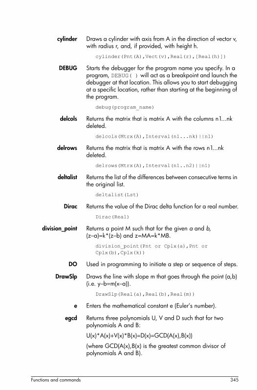
Functions and commands 345
cylinder Draws a cylinder with axis from A in the direction of vector v, with radius r, and, if provided, with height h.
cylinder(Pnt(A),Vect(v),Real(r),[Real(h)])
DEBUG Starts the debugger for the program name you specify. In a program, DEBUG( ) will act as a breakpoint and launch the debugger at that location. This allows you to start debugging at a specific location, rather than starting at the beginning of the program.
debug(program_name)
delcols Returns the matrix that is matrix A with the columns n1...nk deleted.
delcols(Mtrx(A),Interval(n1...nk)||n1)
delrows Returns the matrix that is matrix A with the rows n1...nk deleted.
delrows(Mtrx(A),Interval(n1..n2)||n1)
deltalist Returns the list of the differences between consecutive terms in the original list.
deltalist(Lst)
Dirac Returns the value of the Dirac delta function for a real number.
Dirac(Real)
division_point Returns a point M such that for the given a and b, (z–a)=k*(z–b) and z=MA=k*MB.
division_point(Pnt or Cplx(a),Pnt or Cplx(b),Cplx(k))
DO Used in programming to initiate a step or sequence of steps.
DrawSlp Draws the line with slope m that goes through the point (a,b) (i.e. y–b=m(x–a)).
DrawSlp(Real(a),Real(b),Real(m))
e Enters the mathematical constant e (Euler’s number).
egcd Returns three polynomials U, V and D such that for two polynomials A and B:
U(x)*A(x)+V(x)*B(x)=D(x)=GCD(A(x),B(x))
(where GCD(A(x),B(x) is the greatest common divisor of polynomials A and B).

346 Functions and commands
The polynomials can be provided in symbolic form or as lists. Without a third argument, it is assumed that the polynomials are expressions of x. With a variable as third argument, the polynomials are expressions of it.
egcd((Poly or Lst(A)),(Poly or Lst(B)),[Var])
eigenvals Returns the sequence of eigenvalues of a matrix.
eigenvals(Mtrx)
eigenvects Returns the eigenvectors of a diagonalizable matrix..
eigenvects(Mtrx)
eigVc Returns the eigenvectors of a diagonalizable matrix.
eigVc(Mtrx)
eigVl Returns the Jordan matrix associated with a matrix when the eigenvalues are calculable.
eigVl(Mtrx)
element Shows a point on a curve or a real in an interval.
element((Curve or Real_interval),(Pnt or Real))
ellipse With three points (F1, F2, and M) as arguments, draws an ellipse with foci at F1 and F2 that passes though M. With two points and a real (F1, F2, and a) as arguments, draws an ellipse with foci at F1 and F2 that passes through point M such that MF1+MF2=2a. With one second degree polynomial p(x,y) as argument, draws the ellipse defined when the polynomial is set to equal 0.
ellipse(Pnt(F1),Pnt(F2),(Pnt(M) or Real(a))
or
ellipse(p(x,y))
ELSE Used in programming to introduce the false clause in a conditional statement.
END Used in programming to end a set of statements that should be taken as a single statement.
equilateral_triangle
With three arguments, draws the equilateral triangle ABC of side AB. With four arguments, draws the equilateral triangle ABC in the plane ABP.
equilateral_triangle((Pnt(A) or Cplx),(Pnt(B) or Cplx),[Pnt(P)],[Var(C)])

Functions and commands 347
EVAL Evaluates an expression.
eval(Expr)
evalc Returns an complex expression written in the form real+i*imag.
evalc(Expr)
evalf With one argument, returns the numerical evaluation of it. With a second argument, returns the numerical evaluation of the first argument with the number of significant figures taken from the second argument.
evalf(Expr,[Int])
exact Converts an irrational expression to a rational or real expression.
exact(Expr)
exbisector Draws the exterior bisector of the angle AB-AC given by A,B, and C.
exbisector((Pnt or Cplx(A)),(Pnt or Cplx(B)),(Pnt or Cplx(C)))
excircle Draws the excircle of the triangle ABC.
excircle((Pnt or Cplx(A)),(Pnt or Cplx(B)),(Pnt or Cplx(C)))
EXP Returns the solution to the mathematical constant e to the power of an expression.
exp(Expr)
exponential_regression
Returns the coefficients (a,b) of y=b*a^x, where y is the exponential which best approximates the points whose coordinates are the elements in two lists or the rows of a matrix.
exponential_regression(Lst||Mtrx(A),[Lst])
EXPORT Export. Exports the function FunctionName so that it is globally available and appears on the User menu (D ).
EXPORT(FunctionName)
EXPR Parses the string str into a number or expression.
expr(str)
Examples:

348 Functions and commands
expr("2+3") returns 5.
expr("X+10") returns 100.
(If the variable X has the value 90)
ezgcd Uses the EZ GCD algorithm to return the greatest common divisor of two polynomials with at least two .
ezgcd(Poly,Poly)
f2nd Returns a list consisting of the numerator and denominator of an irreducible form of a rational fraction.
f2nd(RatFrac)
faces Returns the list of the faces of a polygon or polyhedron. Each face is a matrix of n rows and three columns (where n is the number of vertices of the polygon or polyhedron).
faces(Polygon or Polyedr)
factorial Returns the factorial of an integer or the solution to the gamma function for a non-integer.
factorial(Intg(n)||Real(a))
fMax Returns the value of the abscissa at the maximum value of an expression. Without a second argument, it is assumed that it the abscissa is x. With a variable as second argument, it is taken as the abscissa.
fMax(Expr,[Var])
fMin Returns the value of the abscissa at the minimum value of an expression. Without a second argument, it is assumed that it the abscissa is x. With a variable as second argument, it is taken as the abscissa.
fMin(Expr,[Var])
FOR Used in programming in loops for which the number of iterations is known.
format Returns a real number as a string with the indicated format (f=float, s=scientific, e=engineering).
format(Real,Str("f4"||"s5"||"e6"))
fracmod For a given integer n (representing a fraction) and an integer p (the modulus), returns the fraction a/b such that n=a/b(mod p).
fracmod(Intg(n),Intg(p))

Functions and commands 349
froot Returns the list of roots and poles of a rational polynomial. Each root or pole is followed by its multiplicity.
froot(RatPoly)
fsolve Returns the numerical solution of an equation or a system of equations. With the optional third argument you can specify a guess for the solution or an interval within which it is expected that the solution will occur. With the optional fourth argument you can name the iterative algorithm to be used by the solver.
fsolve(Expr,Var,[Guess or Interval],[Method])
function_diff Returns the derivative function of a function.
function_diff(Fnc)
gauss Using the Gauss algorithm, returns the quadratic form of an expression written as a sum or difference of squares of the given in VectVar.
gauss(Expr,VectVar)
GETPIX_C Returns the color of the pixel G with coordinates x,y.
GETPIX_P([G], xposition, yposition)
G can be any of the graphics and is optional. The default is G0, the current graphic.
GF Creates a Galois Field of characteristic p with p^n elements.
GF(Intg(p),Intg(n))
gramschmidt For a basis B of a vector subspace, and a function Sp that defines a scalar product on this vector subspace, returns an orthonormal basis for Sp.
gramschmidt(Basis(B),ScalarProd(Sp))
green Used with display to specify the color of the geometrical object to be displayed.
half_cone Draws a half-cone with vertex A, direction v, half angle t and, if applicable, height h.
half_cone(Pnt(A),Vect(v),Real(t),[Real(h)])
half_line Draws the half-line AB with A as the origin.
half_line((Pnt or Cplx(A)),(Pnt or Cplx(B)))
halftan2hypexp Returns an expression with sin(x), cos(x), tan(x) rewritten in terms of tan(x/2) and sinh(x), cosh(x), tanh(x) rewritten in terms of exp(x).

350 Functions and commands
halftan_hyp2exp(ExprTrig)
halt Used in programming to go into step-by-step debugging mode.
hamdist Returns the Hamming distance between two integers.
hamdist(Intg,Intg)
harmonic_conjugate
Returns the harmonic conjugate of three points or of three parallel or concurrent lines, or returns the line of conjugates of a point with respect to two lines.
harmonic_conjugate(Line or Pnt,Line or Pnt,Line or Pnt)
harmonic_division With three points and a variable as arguments, returns four points that are in a harmonic division. With three lines and a variable as arguments, returns four lines that are in a harmonic division.
harmonic_division(Pnt or Line,Pnt or Line,Pnt or Line,Var)
has Returns 1 if a variable is in an expression, and returns 0 otherwise.
has(Expr,Var)
head Returns the first element of a given vector, sequence or string.
head(Vect or Seq or Str)
Heaviside Returns the value of the Heaviside function for a given real (i.e. 1 if x>=0, and 0 if x<0).
Heaviside(Real)
hexagon Draws a hexagon of side AB in the plane ABP. The other four corners of the hexagon are named according to the given in the third, fourth, fifth and sixth arguments.
hexagon(Pnt or Cplx(A),Pnt or Cplx(B),[Pnt(P)],[Var(C)],[Var(D)],[Var(E)],[Var(F)])
homothety Returns a point A1 such that vect(C,A1)=k*vect(C,A).
homothety(Pnt(C),Real(k),Pnt(A))
hyp2exp Returns an expression with hyperbolic terms rewritten as exponentials.
hyp2exp(ExprHyperb)

Functions and commands 351
hyperbola With three points (F1, F2, and M) as arguments, draws an hyperbola with foci at F1 and F2 that passes though M. With two points and a real (F1, F2, and a) as arguments, draws an hyperbola with foci at F1 and F2 that passes through point M such that |MF1–MF2|=2a. With one second degree polynomial p(x,y) as argument, draws the hyperbola defined when the polynomial is set to equal 0.
hyperbola(Focus(F1),Focus(F2),(Pnt(M) or Real(a)))
iabcuv Returns [u,v] such as au+bv=c for three integers a,b, and c. Note that c must be a multiple of the greatest common divisor of a and b for there to be a solution.
iabcuv(Intg(a),Intg(b),Intg(c))
ibasis Returns the basis of the intersection of two vector spaces.
ibasis(Lst(Vect,..,Vect),Lst(Vect,..,Vect))
icontent Returns the greatest common divisor of the integer coefficients of a polynomial.
icontent(Poly,[Var])
icosahedron Draws an icosahedron with center A, vertex B and such that the plane ABC contains one vertex among the five nearest vertices from B.
icosahedron(Pnt(A),Pnt(B),Pnt(C))
id Returns the solution to the identity function for an expression.
id(Seq)
identity Returns the identity matrix of dimension n.
identity(Intg(n))
iegcd Returns the extended greatest common divisor of two integers.
iegcd(Intg,Intg)
IF Used in programming to begin a conditional statement.
IFERR Executes sequence of commands1. If an error occurs during execution of commands1, execute sequence of commands2. Otherwise, execute sequence of commands3.
IFERR commands1 THEN commands2 [ELSE commands3] END;
IFTE If a condition is satisfied, returns Expr1, otherwise returns Expr2.

352 Functions and commands
IFTE(Cond,Expr1,Expr2)
igcd Returns the greatest common divisor of two integers or two rationals or two polynomials of several .
igcd((Intg(a) or Poly),(Intg(b) or Poly))
ilaplace Returns the inverse Laplace transform of a rational fraction.
ilaplace(Expr,[Var],[IlapVar])
incircle Draws the incircle of triangle ABC.
incircle((Pnt or Cplx(A)),(Pnt or Cplx(B)),(Pnt or Cplx(C)))
inter With two curves or surfaces as arguments, returns the intersection of the curves or surfaces as a vector. With a point as the third argument, returns the intersection of the curves or surfaces close to the point.
inter(Curve,Curve,[Pnt])
interval2center Returns the center of an interval or object.
interval2center(Interval or Real)
inv Returns the inverse of an expression or matrix.
inv(Expr||Mtrx)
inversion Returns point A1 such that A1 is on line CA and mes_alg(CA1*CA)=k.
inversion(Pnt(C),Real(k),Pnt(A))
iPart Returns a real number without its fractional part or a list of real numbers each without its fractional part.
iPart(Real||LstReal)
iquorem Returns the Euclidean quotient and remainder of two integers.
iquorem(Intg(a),Intg(b))
isobarycenter Draws the isobarycenter of the given points.
isobarycenter((Pnt or Cplx),(Pnt or Cplx),(Pnt or Cplx))
isopolygon With two points and n>0, draws a regular polygon with vertices at the two points and abs(n) vertices in total. With three points and n>0, draws a regular polygon with vertices at the first two points and the third point is in the plane of the polygon. With two points and n<0, draws a regular polygon with center at the first point and a vertex at the second point.

Functions and commands 353
With three points and n<0, draws a regular polygon with center at the first point, vertex at the second point and the third point is a point in the plane of the polygon.
isopolygon(Pnt,Pnt,[Pnt],Intg(n))
isosceles_triangle Draws the isosceles triangle ABC. With an angle (t) as the third argument, it is equal to angle AB-AC. With a point (P) as the third argument, the triangle is in the plane formed by A, B and P, and angle AB-AC is equal to angle AB-AP. With a list consisting of a point and an angle as the third argument (t,P), the triangle is in the plane formed by A, B and P, and the angle AB-AC is equal to t.
isosceles_triangle((Pnt or Cplx(A)),(Pnt or Cplx(B)),(Angle(t) or Pnt(P) or Lst(P,t)),[Var(C)])
jacobi_symbol Returns the Jacobi symbol of the given integers.
jacobi_symbol(Intg,Intg)
KILL Used in programming to stop a step-by-step execution with debugging.
laplacian Returns the Laplacian of an expression with respect to a list of .
laplacian(Expr,LstVar)
lcoeff Returns the coefficient of the term of highest degree of a polynomial. The polynomial can be expressed in symbolic form or as a list.
lcoeff(Poly||Lst)
legendre_symbol Returns the Legendre symbol of the given integers.
legendre_symbol(Intg,Intg)
length Returns the length of a list, string or sequence.
length(Lst or Str or Seq)
lgcd Returns the greatest common divisor of a list of integers or polynomials.
lgcd(Seq or Lst)
lin Returns an expression with the exponentials linearized.
lin(Expr)
line_segments Returns the list of the line segments (one line=one segment) of a polyhedron.
line_segments(Polygon or Polyedr(P))
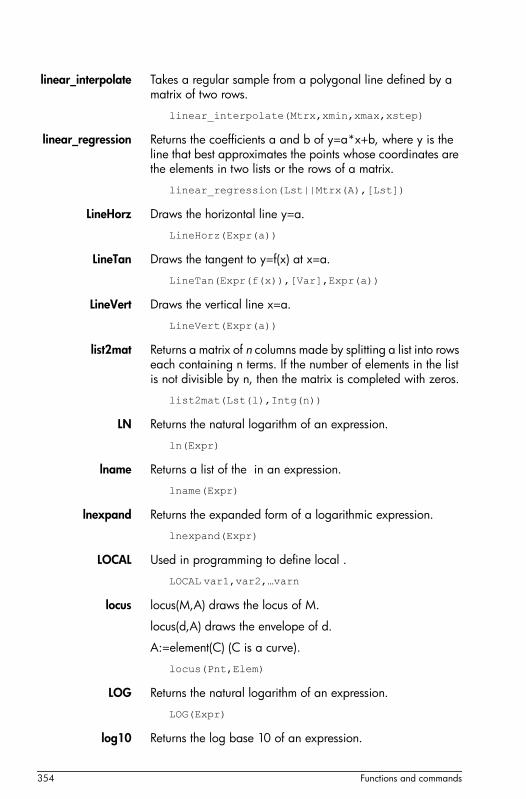
354 Functions and commands
linear_interpolate Takes a regular sample from a polygonal line defined by a matrix of two rows.
linear_interpolate(Mtrx,xmin,xmax,xstep)
linear_regression Returns the coefficients a and b of y=a*x+b, where y is the line that best approximates the points whose coordinates are the elements in two lists or the rows of a matrix.
linear_regression(Lst||Mtrx(A),[Lst])
LineHorz Draws the horizontal line y=a.
LineHorz(Expr(a))
LineTan Draws the tangent to y=f(x) at x=a.
LineTan(Expr(f(x)),[Var],Expr(a))
LineVert Draws the vertical line x=a.
LineVert(Expr(a))
list2mat Returns a matrix of n columns made by splitting a list into rows each containing n terms. If the number of elements in the list is not divisible by n, then the matrix is completed with zeros.
list2mat(Lst(l),Intg(n))
LN Returns the natural logarithm of an expression.
ln(Expr)
lname Returns a list of the in an expression.
lname(Expr)
lnexpand Returns the expanded form of a logarithmic expression.
lnexpand(Expr)
LOCAL Used in programming to define local .
LOCAL var1,var2,…varn
locus locus(M,A) draws the locus of M.
locus(d,A) draws the envelope of d.
A:=element(C) (C is a curve).
locus(Pnt,Elem)
LOG Returns the natural logarithm of an expression.
LOG(Expr)
log10 Returns the log base 10 of an expression.

Functions and commands 355
log10(Expr)
logarithmic_regressio
Returns the coefficients a and b of y=a*ln(x)+b, where y is the natural logarithm that best approximates the points whose coordinates are the elements in two lists or the rows of a matrix.
logarithmic_regression(Lst||Mtrx(A),[Lst])
logb Returns the logarithm of base b of a.
log(a,b)
logistic_regression
Returns y, y', C, y'max, xmax, and R, where y is a logistic function (the solution of y'/y=a*y+b), such that y(x0)=y0 and where [y'(x0),y'(x0+1)...] is the best approximation of the line formed by the elements in the list L.
logistic_regression(Lst(L),Real(x0),Real(y0))
lvar Returns a list of used in an expression.
lvar(Expr)
magenta Used with display to specify the color of the geometrical object to be displayed.
map Applies a function to the elements of the list.
map(Lst,Fnc)
mat2list Returns the list of the terms of a matrix.
mat2list(Mtrx)
matpow Calculates the nth power of a matrix by jordanization
matpow(Mtrx,Intg(n))
MAXREAL Returns the maximum real number that the HP Prime is capable of representing: 9.99999999999E499.
mean Returns the arithmetic mean of a list (with the second argument as pound) or of the columns of a matrix. What does the bit in parentheses mean?
mean(Lst||Mtrx,[Lst])
median Returns the median of a list (with the second argument as pound) or of the columns of a matrix. What does the bit in parentheses mean?
median(Lst||Mtrx,[Lst])
median_line Draws the median line through A of the triangle ABC.

356 Functions and commands
median_line((Pnt or Cplx(A)),(Pnt or Cplx(B)),(Pnt or Cplx(C)))
member Tests if an element is in a list or set. If the element is in the list or set, returns the subsequent element. If the element is not in the list or set, returns 0.
member(Elem(e),(Lst(l) or Set(l)))
midpoint Draws the midpoint of the line segment AB.
midpoint((Pnt or Cplx(A)),(Pnt or Cplx(A)))
MINREAL Returns the minimum real number that the HP Prime is capable of representing: 1E4–99.
MKSA Converts a unit object into a unit object written with the compatible MKSA base unit.
mksa(Unit)
modgcd Uses the modular algorithm to return the greatest common divisor of two polynomials.
modgcd(Poly,Poly)
mRow Multiplies the row n1 of the matrix A by an expression.
mRow(Expr,Mtrx(A),Intg(n1))
mult_c_conjugate If the given complex expression has a complex denominator, returns the expression after both the numerator and the denominator have been multiplied by the complex conjugate of the denominator. If the given complex expression does not have a complex denominator, returns the expression after both the numerator and the denominator have been multiplied by the complex conjugate of the numerator.
mult_c_conjugate(Expr)
mult_conjugate Takes an expression in which the numerator or the denominator contains a square root. If the denominator contains a square root, returns the expression after both the numerator and the denominator have been multiplied by the complex conjugate of the denominator. If the denominator does not contain a square root, returns the expression after both the numerator and the denominator have been multiplied by the complex conjugate of the numerator.
mult_conjugate(Expr)
nDeriv Returns an approximate value of the derivative of an expression at a given point, using f’(x)=(f(x+h)–f(x+h))/2*h.

Functions and commands 357
Without a third argument, the value of h is set to 0.001. With a real as third argument, it is the value of h.
nDeriv(Expr,Var(var),[Real(h)])
NEG Unary minus. Enters the negative sign.
normal Returns the expanded irreducible form of an expression.
normal(Expr)
normalize Returns a vector divided by its l2 norm (where the l2 norm is the square root of the sum of the squares of the vector’s coordinates).
normalize(Lst||Cplx)
NOT Returns the logical inverse of a Boolean expression.
not(Boolean)
NTHROOT Gives the expression for calculating the nth root of a number.
octahedron Draws an octahedron with center A and vertex B and such that the plane ABC contains four vertices.
octahedron(Pnt(A),Pnt(B),Pnt(C))
odd Returns 1 if a given integer is odd, and returns 0 otherwise.
odd(Intg(n))
open_polygon Draws a polygonal line with vertices at the elements of the given list.
open_polygon(LstPnt||LstCplx)
OR Logical Or.
expr1 OR expr2
Example:
3+1==4 OR 8 < 5 returns 1.
order_size Returns the remainder (O term) of a series expansion: limit(x^a*order_size(x),x=0)=0 if a>0.
order_size(Expr)
orthocenter Shows the orthocenter of the triangle made with three points.
orthocenter((Pnt or Cplx),(Pnt or Cplx),(Pnt or Cplx))
orthogonal With a point (A) and a line (BC) as arguments, draws the orthogonal plane of the line that passes through the point.

358 Functions and commands
With a point (A) and a plane (BCD) as arguments, draws the orthogonal line of the plane that passes through the point.
orthogonal(Pnt(A),(Line(BC) or Plane(BCD))
pa2b2 Takes a prime integer n congruent to 1 modulo 4 and returns [a,b] such that a^2+b^2=n.
pa2b2(Intg(n))
pade Returns the Pade approximation i.e. a rational fraction P/Q such that P/Q=Xpr mod x^(n+1) or mod N with degree(P)<p.
pade(Expr(Xpr), Var(x), (Intg(n) || Poly(N)), Intg(p))
parabola With two points (F, A) as arguments, draws a parabola of focus F and top A. With three points (F, A and P) as arguments, draws a parabola with focus F and top A in the plane ABP. With a complex (A) and a real (c) as arguments, draws a parabola of equation y=yA+c*(x–xA)^2. With one second degree polynomial (P(x,y)) as argument, draws the parabola when the polynomial is set to equal 0.
parabola(Pnt(F)||Pnt(xA+i*yA),Pnt(A)||Real(c),[Pnt(P)])
parallel With a point and a line as arguments, draws the line through the point that is parallel to the given line. With a point and a plane as arguments, draws the plane through the point that is parallel to the given plane. with a point and two lines as arguments, draws the plane through the point that is parallel to the plane made by the two given lines.
parallel(Pnt or Line,Line or Plane,[Line])
parallelepiped Draws a parallelepiped with sides AB, AC, and AD. The faces of the parallelepiped are parallelograms.
parallelepiped(Pnt(A),Pnt(B),Pnt(C),Pnt(D))
parallelogram Draws the parallelogram ABCD such that vector(AB)+vector(AD)=vector(AC).
parallelogram(Pnt(A)||Cplx,Pnt(B)||Cplx,Pnt(C)||Cplx,[Var(D)])
perimeterat Displays the perimeter at point z0 of a circle or polygon. A legend is provided.
perimeterat(Polygon,Pnt||Cplx(z0))
perimeteratraw Displays the perimeter at point z0 of a circle or polygon.
perimeteratraw(Polygon,Pnt||Cplx(z0))

Functions and commands 359
perpen_bisector Draws the bisection (line or plane) of the segment AB.
perpen_bisector((Pnt or Cplx(A)),(Pnt or Cplx(B)))
perpendicular With a point and a line as arguments, returns the line that is orthogonal to the given line and that passes through the given point. With a line and a plane as arguments, draws the plane that is orthogonal to the given plane and that contains the given line.
perpendicular((Pnt or Line),(Line or Plane))
PI Inserts pi.
PIECEWISE Takes as arguments pairs consisting of a condition and an expression. Each of these pairs defines a subfunction of the piecewise function and the domain over which it is active.
piecewise(Cond1,Expr1,..,Cond2p,Expr2p,[Expr2p+1])
plane With three points as arguments, draws the plane made by the three points. With a point and a line as arguments, draws the plane made by the point and the line. With an equation as argument, draws the plane corresponding to the equation in 3D space.
plane(Pnt or Eq, [Pnt or Line],[Pnt])
plotinequation Draws the points of the plane whose coordinates satisfy the inequations of two
plotinequation(Expr,[x=xrange,y=yrange],[xstep],[ystep])
plotparam With a complex (a(t)+i*b(t)) and a list of values for the variable (t) as arguments, draws the parametric representation of the curve defined by x=a(t) and y=g(t) over the interval specified in the second argument. With a list of expressions of two (a(u,v),b(u,v),c(u,v)) and a list of values for the (u=u0...u1,v=v0...v1) as arguments, draws the surface defined by x=a(u,v), y=b(u,v), and z=c(u,v) over the intervals specified by in the second argument.
plotparam(Cplx||Lst,Var||Lst(Var))
plotpolar For an expression f(x), draws the polar curve r=f(x) for x over the interval VarMin to VarMax.
plotpolar(Expr,Var,VarMin,VarMax)
plotseq Displays the pth terms of the sequence u(0)=a,u(n)=f(u(n–1)).

360 Functions and commands
plotseq(Expr(f(Var)),Var=[a,xm,xM],Intg(p))
point With a complex as argument, plots it. With the coordinates of a point in three dimensions as argument, plots it.
point(Cplx||Vect)
polar Returns the line of the conjugated points of A with respect to a circle.
polar(Crcle,Pnt or Cplx(A))
polar_coordinates Returns the list of the norm and of the argument of the affix of a point, complex number or list of rectangular coordinates.
polar_coordinates(Pnt or Cplx or LstRectCoord)
polar_point Returns the point with polar coordinates r and t.
polar_point(Real(r),Real(t))
pole Returns the point for which the line is polar with respect to the circle.
pole(Crcle,Line)
POLYCOEF Returns the coefficients of a polynomial with roots given in the vector argument.
polyCoef(Vect)
POLYEVAL Evaluates a polynomial given by its coefficients at x0.
polyEval(Vect,Real(x0))
polygon Draws the polygon whose vertices are elements in a list.
polygon(LstPnt||LstCplx)
polygonplot Draws the polygons made by joining the points (xk,yk), where xk=element row k column 0 and yk=element row k column j (for j fixed and for k=0...nrows).
polygonplot(Mtrx)
polygonscatterplot
Draws the points (xk,yk) and the polygons made by joining the points (xk,yk), where xk=element row k column 0 and yk=element row k column j (for j fixed and for k=0...nrows).
polygonscatterplot(Mtrx)
polyhedron Draws a convex polyhedron whose vertices are the points in the sequence.
polyhedron(SeqPnt(A,B,C...))

Functions and commands 361
polynomial_regression
Returns the coefficients (an,...a1,a0) of y=an*x^n+..a1x+a0), where y is the nth order polynomial which best approximates the points whose coordinates are the elements in two lists or the rows of a matrix.
polynomial_regression(Lst||Mtrx(A),[Lst],Intg(n))
POLYROOT Returns the zeros of the polynomial given as argument (either as symbolic expression or as a vector of coefficients).
POLYROOT(P(x) or Vect)
potential Returns a function whose gradient is the vector field defined by Vect(V) and VectVar.
potential(Vect(V),VectVar)
power_regression Returns the coefficients (m,b) of y=b*x^m, where y is the monomial which best approximates the points whose coordinates are the elements in two lists or the rows of a matrix.
power_regression(Lst|Mtrx(A),[Lst])
powerpc Returns the real number d^2–R^2, where d is the distance between the point and the center of the circle, and R is the radius of the circle.
powerpc(Crcle,Pnt or Cplx)
prepend Adds an element to the beginning of a list.
prepend(Lst,Elem)
primpart Returns a polynomial divided by the greatest common divisor of its coefficients.
primpart(Poly,[Var])
prism Draws a prism whose base is the plane ABCD and whose edges are parallel to the line made by A and A1.
prism(LstPnt([A,B,C,D]),Pnt(A1))
product With an expression as the first argument, returns the product of solutions when the variable in the expression is substituted from a to b with step p. If p is not provided, it is taken as 1. With a list as the first argument, returns the product of the values in the list. With a matrix as the first argument, returns the element-by-element product of the matrix.
product(Expr||Lst,[Var||Lst],[Intg(a)],[Intg(b)],[Intg(p)])

362 Functions and commands
projection Returns the orthogonal projection of the point on the curve.
projection(Curve,Pnt)
propfrac Returns a fraction or rational fraction A/B simplified to Q+r/B, where R<B or the degree of R is less than the degree of B.
propfrac(Frac or RatFrac)
ptayl Returns the Taylor polynomial Q such as P(x)=Q(x–a).
ptayl(Poly(P(var)),Real(a),[Var])
purge Unassigns a variable name.
purge(Var)
pyramid With three points as arguments, draws the pyramid with a face in the plane of the three points and with two vertices at the first and second points. With four points as arguments, draws the pyramid with vertices at the four points.
pyramid(Pnt(A),Pnt(B),Pnt(C),[Pnt(D)])
q2a Returns the matrix of a quadratic form with respect to the given in VectVar.
q2a(QuadraForm,VectVar)
quadrilateral Draws the quadrilateral ABCD.
quadrilateral(Pnt(A)||Cplx,Pnt(B)||Cplx,Pnt(C)||Cplx,Pnt(D)||Cplx)
quantile Returns the quantile of the elements of a list corresponding to p (0<p<1).
quantile(Lst(l),Real(p))
quartile1 Returns the first quartile of the elements of a list or the columns of a matrix.
quartile1(Lst||Mtrx,[Lst])
quartile3 Returns the third quartile of the elements of a list or the columns of a matrix.
quartile3(Lst||Mtrx,[Lst])
quartiles Returns the minimum, first quartile, median, third quartile, and maximum of the elements of a list or the columns of a matrix.
quartiles(Lst||Mtrx,[Lst])
quorem Returns the quotient and remainder of the Euclidean division (by decreasing power) of two polynomials. The polynomials

Functions and commands 363
can be expressed as vectors of their coefficients or in symbolic form.
quorem((Vect or Poly),(Vect or Poly),[Var])
QUOTE Returns an expression unevaluated.
quote(Expr)
radical_axis Returns the line which is the locus of points at which tangents drawn to two circles have the same length.
radical_axis(Crcle,Crcle)
randexp Returns a random real according to the exponential distribution of parameter a>0.
randexp(Real(a))
randperm Returns a random permutation of [0,1,2,...,n–1].
randperm(Intg(n))
ratnormal Rewrites an expression as an irreducible rational fraction.
ratnormal(Expr)
reciprocation Returns the list where a point is replaced with its polar or a line is replaced with its pole with respect to the circle.
reciprocation(Crcle,Lst(Pnt,Line))
rectangle Draws the rectangle ABCD, where, if k is provided, AD=k*AB if k>0, and where, if k and P are provided, the rectangle is in the plane ABP with AD=AP and AD=k*AB.
rectangle(Pnt(A)||Cplx,Pnt(B)||Cplx,Real(k)||Pnt(P)||Lst(P,k),[Var(D)],[Var(C)])
rectangular_coordinat
Returns the list of the abscissas and of the ordinates of points given by a list of their polar coordinates.
rectangular_coordinates(LstPolCoord)
red Used with display to specify the color of the geometrical object to be displayed.
reduced_conic Takes a conic expression and a vector of , and returns the origin of the conic, the matrix of a basis in which the conic is reduced, 0 or 1 (0 if the conic is degenerate), the reduced equation of the conic, and a vector of the conic’s parametric equations.
reduced_conic(Expr,[LstVar])

364 Functions and commands
ref Returns the solution to a system of linear equations written in matrix form.
ref(Mtrx(M))
reflection With a line (D) and a point (C) as arguments, returns the reflection of the point across the line (i.e. the line is taken as a line of symmetry). With a point (A) and a curve (C) as arguments, returns the reflection of the curve about the point (i.e. the point is taken as the point of symmetry).
reflection((Pnt(A) or Line(D)),(Pnt(C) or Curve(C)))
remove Returns a list with the elements that satisfy the Boolean function removed.
remove(FncBool(f)||e,Lst(l))
reorder Reorders the in an expression according to the order given in LstVar.
reorder(Expr,LstVar)
REPEAT Used in programming to indicate a statement or statements that should be repeated until a given condition is true.
residue Returns the residue of an expression at a.
residue(Expr,Var(v),Cplx(a))
restart Purges all the .
restart(NULL)
resultant Returns the resultant (i.e. the determinant of the Sylvester matrix) of two polynomials.
resultant(Poly,Poly,Var)
RETURN Used in programming return a value of a function at a certain point.
return(Expr)
revlist Returns a list with the elements in reverse order.
revlist(Lst)
rhombus With two points (A and B) and an angle (a) as arguments, draws the rhombus ABCD such that the angle AB-AD=a. With three points as arguments (A, B and P), draws the rhombus ABCD in the plane ABP such that angle AB-AD=angle AB-AP.
rhombus(Pnt(A)||Cplx,Pnt(B)||Cplx,Angle(a)||Pnt(P)||Lst(P,a)),[Var(C)],[Var(D)])

Functions and commands 365
right_triangle With two points (A and B) and a real (k) as arguments, draws right-angled triangle such ABC such that AC=k*AB. With three points (A, B and P) as arguments, draws the right-angled triangle ABC in the plane ABP and such that AC=AP.
right_triangle((Pnt(A) or Cplx),(Pnt(B) or Cplx),(Real(k) or Pnt(P) or Lst(P,k)),[Var(C)])
romberg Uses Romberg’s method to return the approximate value of the integral of the expression over the interval a to b.
romberg(Expr(f(x)),Var(x),Real(a),Real(b))
rotation With a point (B), an angle (a1) and another point (A) as arguments, returns the result of rotating the second point by the angle about the center of rotation given by the first point. With a line (Dr3), an angle (a1) and a curve as arguments, returns the result of rotating the curve by the angle about the axis of rotation given by the line.
rotation((Pnt(B) or Cplx or Dr3),Angle(a1),(Pnt(A) or Curve))
row Returns the row n or the sequence of the rows n1...n2 of the matrix A.
row(Mtrx(A),Intg(n)||Interval(n1..n2))
rowAdd Returns the matrix obtained from matrix A after the n2th row is replaced by the sum of the n1th row and the n2th row.
rowAdd(Mtrx(A),Intg(n1),Intg(n2))
rowDim Returns the number of rows of a matrix.
rowDim(Mtrx)
rowSwap Returns the matrix obtained from matrix A after the n1th row and the n2th row are swapped.
rowSwap(Mtrx(A),Intg(n1),Intg(n2))
rsolve Returns the values of a recurrent sequence or a system of recurrent sequences.
rsolve((Expr or LstExpr),(Var or LstVar),(InitVal or LstInitVal))
segment Draws a line segment connecting two points.
segment((Pnt or Cplx),(Pnt or Cplx),[Var],[Var])

366 Functions and commands
select Returns a list with only the elements that satisfy the Boolean function remaining.
select(FncBool(f),Lst(l))
seq With an expression and two integers (a and b) as arguments, returns the sequence obtained when the expression is evaluated within the interval given by a and b. With an expression and three integers (a, b and p) as arguments, returns the sequence obtained when the expression is evaluated with step of p within the interval given by a and b. With an expression and three integers (n, a and b) as arguments, returns the sequence obtained when the expression is evaluated n times of equal spacing within the interval given by a and b.
seq(Expr,Intg(n)||Var(var),[Intg(a)],[Intg(b)],[Intg(p)])
seqsolve Returns the value of a recurrent sequence or a system of recurrent sequences (u_{n+1}=f(u_n) or u_{n+2}=f(u_{n+1},u_n)...).
seqsolve((Expr or LstExpr),(Var or LstVar),(InitVal or LstInitVal))
shift_phase Returns the result of applying a phase shift of pi/2 to a trigonometric expression.
shift_phase(Expr)
signature Returns the signature of a permutation.
signature(Permut)
similarity With two points (B and A), a real (k) and an angle (a1) as arguments, returns a point that is the point similar to A across center B with angle a1 and with scaling coefficient k. With an axis (Dr3), a real (k) an angle (a1) and a point (A) as arguments, returns a point that is the point similar to A across the axis given by the line with angle a1 and with scaling coefficient k.
similarity(Pnt(B) or Dr3,Real(k),Angle(a1),Pnt(A))
simult Returns the solution to a system of linear equations or several systems of linear equations presented in matrix form. In other words, in the case of one system of linear equations, takes a matrix A and a column matrix B, and returns column matrix X such A*X=B.
SIN Sine: sinx.

Functions and commands 367
SIN(value)
sincos Returns an expression with the complex exponentials rewritten in terms of sin and cos.
sincos(Expr)
single_inter With two curves or two surfaces as arguments, returns one of the intersections of the two curves or surfaces. With to curves or surfaces and a point or list of points as arguments, returns an intersection of the curves or surfaces that is nearest to the point or not in the list of points.
single_inter(Curve,Curve,[Pnt(A)||LstPnt(L)])
slopeat Displays the value at point z0 of the slope of the line or segment d. A legend is provided.
slopeat(Line,Pnt||Cplx(z0))
slopeatraw Displays the value at point z0 of the slope of the line or segment d.
slopeatraw(Line, Pnt||Cplx(z0))
sphere With two points as arguments, draws the sphere of diameter made by the line from one point to another. With a point and a real as arguments, draws the sphere with center at the point and radius given by the real.
sphere((Pnt or Vect),(Pnt or Real))
spline Returns the natural spline through the points given by two lists. The polynomials in the spline are in variable x and of degree d.
spline(Lst(lx),Lst(ly),Var(x),Intg(d))
sqrt Returns the square root of an expression.
sqrt(Expr)
square Draws the square of side AB in the plane ABP.
square((Pnt(A) or Cplx),(Pnt(B) or Cplx),[Pnt(P),Var(C),Var(D)])
stddev Returns the standard deviance of the elements in a list with the second argument as pound or returns the list of standard deviances of the columns of a matrix. What does the “pound” mean?
stddev(Lst||Mtrx,[Lst])

368 Functions and commands
stddevp Returns the population standard deviance of the elements in a list with the second argument as pound or returns the list of standard deviances of the columns of a matrix. What does the “pound” mean?
stddevp(Lst||Mtrx,[Lst])
STEP Used in prgramming to indicate the step in an iteration or the step size of an incrementation.
sto Stores a real or string in a variable.
sto((Real or Str),Var)
sturmseq Returns the Sturm sequence for a polynomial or a rational fraction.
sturmseq(Poly,[Var])
subMat Extracts from a matrix a sub matrix with first element=A[n1,n2] and last element=A[n3,n4].
subMat(Mtrx(A),Intg(n1),Intg(n2),Intg(n3),Intg(n4))
suppress Returns a list without the nth element.
suppress(Lst,Intg(n))
surd Returns an expression to the power of 1/n.
surd(Expr,Intg(n))
sylvester Returns the Sylvester matrix of two polynomials.
sylvester(Poly,Poly,Var)
table Defines an array where the indexes are strings or real numbers.
table(SeqEqual(index_name=element_value))
tail Returns a list or sequence or string without its first element.
tail(Lst or Seq or Str)
TAN Tangent: tan(x).
tan(value)
tan2cossin2 Returns an expression with tan(x) rewritten as (1–cos(2*x))/sin(2*x).
tan2cossin2(Expr)
tan2sincos2 Returns an expression with tan(x) rewritten as sin(2*x)/(1+cos(2*x)).

Functions and commands 369
tan2sincos2(Expr)
tangent With a curve as argument, draws the tangent line to the curve at point A. With a surface as argument, draws the tangent plane to the surface at point A.
tangent(Curve or surface(C),Pnt(A))
THEN Used in programming to introduce a statement dependent on a conditional statement.
TO Used in programming in a loop when expressing the range of values of a variable for which a statement should be executed.
translation With a vector and a point as arguments, returns the point translated by the vector. with two points as arguments, returns the second point translated by the vector from the origin to the first point.
translation(Vect,Pnt(C))
transpose Returns a matrix transposed (without conjugation).
transpose(Mtrx)
triangle Draws a triangle with vertices at the three points.
triangle((Pnt or Cplx),(Pnt or Cplx),(Pnt or Cplx))
trunc Returns a value or a list of values truncated to n decimal places. If n is not provided, it is taken as 0. Accepts complex numbers.
trunc(Real||LstReal,Int(n))
tsimplify Returns an expression with transcendentals rewritten as complex exponentials.
tsimplify(Expr)
type Returns the type of an expression (e.g. list, string).
type(Expr)
UFACTOR Factorizes a unit in a unit object.
ufactor(Unit,Unit)
unapply Returns the function defined by an expression and a variable.
unapply(Expr,Var)
UNTIL Used in programming to indicate the conditions under which a statement should stop being executed.

370 Functions and commands
USIMPLIFY Simplifies a unit in a unit object.
usimplify(Unit)
valuation Returns the valuation (degree of the term of lowest degree) of a polynomial. With only a polynomial as argument, the valuation returned is for x. With a variable as second argument, the valuation is performed for it.
valuation(Poly,[Var])
variance Returns the variance of a list with the second argument as pound or the list of variances of the columns of a matrix.
variance(Lst||Mtrx,[Lst])
vector With one point as argument, defines a vector from the origin to the point. With two points as arguments, defines a vector from the first point to the second point. With a point and a vector as arguments, defines a vector beginning from the point and with direction and magnitude of the vector.
vector(Pnt,Pnt||Pnt,Vect).
vertices Returns the list of the vertices of a polygon or polyhedron.
vertices(Polygon or Polyedr)
vertices_abca Returns the closed list [A,B,...A] of the vertices of a polygon or polyhedron.
vertices_abca(Polygon or Polyedr)
vpotential Returns U such as curl(U)=V.
vpotential(Vect(V),LstVar)
when Used to introduce a conditional statement.
WHILE Used to indicate the conditions under which a statement should be executed.
XOR Exclusive or. Returns 1 if the first expression is true and the second expression is false or if the first expression is false and the second expression is true. Returns 0 otherwise.
xor(Expr1,Expr2)
yellow Used with display to specify the color of the geometrical object to be displayed.
zip Applies a bivariate function to the elements of two lists. Without the default value its length is the minimum of the lengths of the two lists and the shorter list is padded with the default value.

Functions and commands 371
zip(Fnc2d(f),Lst(l1),Lst(l2),[Val(default)])
| Substitutes a value for a variable in an expression.
|(Expr,Var(v1)=value(a1)[,v2=a2,...])
2 Returns the square of an expression.
(Expr)2
Inserts pi.
10^ What does this one do?
Inserts a template for a partial derivative expression.
Inserts a template for a summation expression.
Inserts a minus sign.
Inserts a square root sign.
Inserts a template for an antiderivative expression.
Inserts a not-equal-to sign.
Inserts a less-than-or-equal-to sign.
Inserts a greater-than-or-equal-to sign.
Evaluates the expression then stores the result in variable var. Note that cannot be used with the graphics G0–G9. See the command BLIT.
expression var
i Inserts the imaginary number i.-1 Returns the inverse of an expression.
(Expr)–1
Creating your own functionsYou can create your own function by writing a program (see chapter 26) or by using the simpler DEFINE functionality. Functions you create yourself appear on the User menu (one of the Toolbox menus).
Suppose you wanted to create the function SINCOS(A,B)=SIN(A)+COS(B)+C.

372 Functions and commands
1. Press Sd (Define).
2. In the Name field, enter a name for the function—for example, SINCOS—and tap
.
3. In the Function field, enter the function.
eAA>+fAB>AC
New fields appear below your function, one for each potential parameter it. will take. You need to decide which ones are to be parameters when the function is called. In this example, we’ll make A and B parameters. The value of C will be provided by global variable C (which by default is zero).
4. Make sure that A and B are selected and C is not.
5. Tap .
You can run your function by entering it on the entry line in Home view, or be selecting it from the USER menu. You enter the value for each variable you chose to be a parameter. In this example. we chose A and B to be parameters. Thus you might enter SINCOS(0.5, 0.75).

Variables 373
21
Variables
Variables are placeholders for objects (such as function definitions, numbers, matrices, the results of calculations, and the like). Some are built-in and cannot be deleted. But you can also create your own.
Many built-in variables are automatically assigned objects as a result of some operation (such as defining a polar function, performing a calculation, or setting an option). For example, if you define a polar function, that definition is assigned to variable named R0 to Rn. If you use the Function app to find the slope of a curve at some x-value, the slope is assigned to a variable named Slope. And if you choose binary as the base for integer arithmetic, a built-in variable named Base is given the value 0. If you had chosen octal instead, Base would have been given the value 1.
Creating variables Variables you create are assigned whatever value you give them. You can assign a value to certain built-in variables (such as the Home variables). You can also create your own variables. Example 1 below gives an example of assigning a value to a built-in variable, and example 2 illustrates how to create a variable and assign a value to it
Example 1: To assign 2 to the built-in variable A:
Szj AaE
Your stored value appears as shown at the right. If you then wanted to multiply your stored value by 5, you could enter:
Aas5E

374 Variables
To assign an object to a built-in variable, it is important that you choose a variable that matches the type of object. For example, you cannot assign a complex number to the variables A through Z. These are reserved fro real numbers. Complex numbers need to be assigned to variables Z0 through Z9. Likewise, matrices can only be assigned to the built-in variables M0 through M9. See “Home variables” on page 377 for more information.
You can also take advantage of the built-in variables in CAS view. However, the built-in CAS variables must be entered in lowercase: a–z.
Example 2: You can create your own variables—in Home view and in CAS view. For example, suppose you want to create a variable called ME and assign 2 to it. You would enter:
Szj AQAcE
A message appears asking if you want to create a variable called ME. Tap or press E to confirm your intention. You can now use that variable in subsequent calculations: ME*3 will yield 303, for example.
You can also create variables by entering [variable name]:=[object]. For example, entering AxAoAtAwS.55Eassigns 55 to the variable YOU. You can now use that variable in subsequent calculations: YOU+60 will yield 115, for example.
Using variables to change settings
Just as you can assign values to variables you create yourself, you can assign values to certain built-in variables. You could modify Home settings on the Home Settings screen (SH). But you can also modify a Home setting from Home view by assigning a value to the variable that represents that setting. For example, entering 0 Base E in Home view forces the setting for the integer base to binary. (A value of 1 would force it to octal, 2 to decimal, and 3 to hex.) Another example: you can change the angle measure setting from radians to
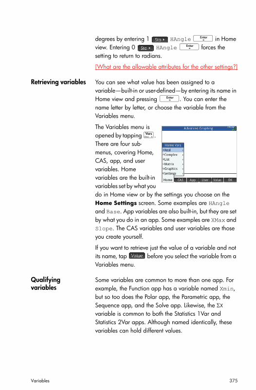
Variables 375
degrees by entering 1 HAngle E in Home view. Entering 0 HAngle E forces the setting to return to radians.
[What are the allowable attributes for the other settings?]
Retrieving variables You can see what value has been assigned to a variable—built-in or user-defined—by entering its name in Home view and pressing E. You can enter the name letter by letter, or choose the variable from the Variables menu.
The Variables menu is opened by tapping a. There are four sub-menus, covering Home, CAS, app, and user variables. Home variables are the built-in variables set by what you do in Home view or by the settings you choose on the Home Settings screen. Some examples are HAngle and Base. App variables are also built-in, but they are set by what you do in an app. Some examples are XMax and Slope. The CAS variables and user variables are those you create yourself.
If you want to retrieve just the value of a variable and not its name, tap before you select the variable from a Variables menu.
Qualifying variables
Some variables are common to more than one app. For example, the Function app has a variable named Xmin, but so too does the Polar app, the Parametric app, the Sequence app, and the Solve app. Likewise, the X variable is common to both the Statistics 1Var and Statistics 2Var apps. Although named identically, these variables can hold different values.

376 Variables
If you attempt to retrieve a variable that is used in more than one app by entering just its name in Home view, you will get the value that was last calculated for that variable. This might not be the value that you want. To ensure you get the right value, you need to qualify the variable with the name of the app that generated it. In the example at the right, the variable X was entered, but it returned the value of that variable as it was calculated in the Statistics 1Var app (the first entry). However, it was the value of the variable as it was calculated in the Statistics 2Var app that was sought. To retrieve that value, the variable name had to be qualified by prefixing it with the name of the app that generated it: Statistics_2Var followed by a period (the second entry).
Note the syntax required:
app_name.variable_name
Spaces are not allowed in an app name and must be represented by the underscore character: SX. The app can be a built-in app or one you have crated based on a built-in app. The name of a built-in variable must match a name listed in the Home variables or App variables tables below.
Tip Non-standard characters in variables name—such as and —can be entered by selecting them from the special symbols palette: Sr.

Variables 377
Home variablesThe Home variables are accessed by pressing a and tapping .
Category Available names
Real A to Z and
For example, 7.45 A
Complex Z0 to Z9
For example, 2+3×i Z1 or
(2,3) Z1 (depending on your Complex number settings)
List L0 to L9
For example, {1,2,3} L1.
Matrix M0 to M9
Store matrices and vectors in these variables.
For example, [[1,2],[3,4]] M1.
Graphics G0 to G9
Settings HAngle
HFormat
HDigits
HComplex
Date
Time
Language
Entry
Integer
Base
Bits
Signed

378 Variables
App variablesThe app variables are accessed by pressing a and tapping . They are grouped below by app. (You can find then grouped by view—Symbolic, Numeric, Plot, —in “Variables and Programs” on page 492.)
Note that if you have customized a built-in app, your app will appear on the App variables menu under the name you gave it. You access the variables in a customized app in the same way that you access the variables in built-in apps.
Function app variables
Category Names
Resultsa AreaExtremumIsect
RootSlope
Symbolic F1F2F3F4F5
F6F7F8F9F0
Plot AxesCursorGridDotsGridLinesLabelsMethodRecenterXmax
XminXtickXzoomYmaxYminYtickYzoom
Numeric NumStartNumStepAutomaticNumIndep
NumTypeNumZoomBuildYourOwn
Modes AAngleAComplex
ADigitsAFormat

Variables 379
Geometry app variables
Spreadsheet app variables
a. The Results variables contain the last value found by the Signed Area, Extremum, Intersection, Root, and Slope functions respectively.
Category Names
Numeric XMinYMin
XMax
Modes AAngleAComplex
ADigitsAFormat
Category Names
Numeric ColWidthRowCell
RowHeightCol
Modes AAngleAComplex
ADigitsAFormat

380 Variables
Advanced Graphing app variables
Solve app variables
Category Names
Symbolic S1S2S3S4S5
S6S7S8S9S0
Plot AxesCursorGridDotsGridLinesLabelsMethodRecenterXmax
XminXtickXzoomYmaxYminYtickYzoom
Numeric NumXStartNumYStartNumXStepNumYStepNumIndep
NumTypeNumXZoomNumYZoomAutomaticBuildYourOwn
Modes AAngleAComplex
ADigitsAFormat
Category Names
Symbolic E1E2E3E4E5
E6E7E8E9E0
Plot AxesCursorGridDotsGridLinesLabelsMethodRecenterXmax
XminXtickXzoomYmaxYminYtickYzoom

Variables 381
Statistics 1Var app variables
Modes AAngleAComplex
ADigitsAFormat
Category Names
Results [explained below]
NbItemMinQ1MedQ3Max
XX2MeanXsXXserrX
Symbolic H1H2H3H4H5
H1TypeH2TypeH3TypeH4TypeH5Type
Plot AxesCursorGridDotsGridLinesHminHmaxHwidthLabelsRecenter
XmaxXminXtickXzoomYmaxYminYtickYzoom
Numeric D1D2D3D4D5
D6D7D8D9D0
Modes AAngleAComplex
ADigitsAFormat
Category Names (Continued)

382 Variables
Results
NbItem Contains the number of data points in the current 1-variable analysis (H1-H5).
Min Contains the minimum value of the data set in the current 1-variable analysis (H1-H5).
Q1 Contains the value of the first quartile in the current 1-variable analysis (H1-H5).
Med Contains the median in the current 1-variable analysis (H1-H5).
Q3 Contains the value of the third quartile in the current 1-variable analysis (H1-H5).
Max Contains the maximum value in the current 1-variable analysis (H1-H5).
X Contains the sum of the data set in the current 1-variable analysis (H1-H5).
X2 Contains the sum of the squares of the data set in the current 1-variable analysis (H1-H5).
MeanX Contains the mean of the data set in the current 1-variable analysis (H1-H5).
sX Contains the sample standard deviation of the data set in the current 1-variable analysis (H1-H5).
X Contains the population standard deviation of the data set in the current 1-variable analysis (H1-H5).
serrX Contains the standard error of the data set in the current 1-variable analysis (H1-H5).

Variables 383
Statistics 2Var app variables
Results
NbItem Contains the number of data points in the current 2-variable analysis (S1-S5).
Category Names
Results[explained below]
NbItemCorrCoefDetsCovCovXYMeanXXX2
sXXserrXMeanYYY2sYYserrY
Symbolic S1S2S3S4S5
S1TypeS2TypeS3TypeS4TypeS5Type
Plot AxesCursorGridDotsGridLinesLabelsMethodRecenterXmax
XminXtickXzoomYmaxYminYtickYzoom
Numeric C1C2C3C4C5
C6C7C8C9C0
Modes AAngleAComplex
ADigitsAFormat

384 Variables
Corr Contains the correlation coefficient from the latest calculation of summary statistics. This value is based on the linear fit only, regardless of the fit type chosen.
CoefDet Contains the coefficient of determination from the latest calculation of summary statistics. This value is based on the fit type chosen.
sCov Contains the sample covariance of the current 2-variable statistical analysis (S1-S5).
Cov Contains the population covariance of the current 2-variable statistical analysis (S1-S5).
XY Contains the sum of the X·Y products for the current 2-variable statistical analysis (S1-S5).
MeanX Contains the mean of the independent values (X) of the current 2-variable statistical analysis (S1-S5).
X Contains the sum of the independent values (X) of the current 2-variable statistical analysis (S1-S5).
X2 Contains the sum of the squares of the independent values (X) of the current 2-variable statistical analysis (S1-S5).
sX Contains the sample standard deviation of the independent values (X) of the current 2-variable statistical analysis (S1-S5).
X Contains the population standard deviation of the independent values (X) of the current 2-variable statistical analysis (S1-S5).
serrX Contains the standard error of the independent values (X) of the current 2-variable statistical analysis (S1-S5).
MeanY Contains the mean of the dependent values (Y) of the current 2-variable statistical analysis (S1-S5).
Y Contains the sum of the dependent values (Y) of the current 2-variable statistical analysis (S1-S5).

Variables 385
Y2 Contains the sum of the squares of the dependent values (Y) of the current 2-variable statistical analysis (S1-S5).
sY Contains the sample standard deviation of the dependent values (Y) of the current 2-variable statistical analysis (S1-S5).
Y Contains the population standard deviation of the dependent values (Y) of the current 2-variable statistical analysis (S1-S5).
serrY Contains the standard error of the dependent values (Y) of the current 2-variable statistical analysis (S1-S5).
Inference app variables
Results
CritScore Contains the value of the Z- or t-distribution associated with the input -value
Category Names
Results[explained below]
ResultTestScoreTestValueProb
CritScoreCritVal1CritVal2DF
Symbolic AltHypMethod
Type
Numeric AlphaConfMean1Mean2n1n200
Pooleds1s212x1x2
Modes AAngleAComplex
ADigitsAFormat

386 Variables
CritVal1 Contains the lower critical value of the experimental variable associated with the negative TestScore value which was calculated from the input -level.
CritVal2 Contains the upper critical value of the experimental variable associated with the positive TestScore value which was calculated from the input -level.
DF Contains the degrees of freedom for the t-tests.
Prob Contains the probability associated with the TestScore value.
Result For hypothesis tests, contains 0 or 1 to indicate rejection or failure to reject the null hypothesis.
TestScore Contains the Z- or t-distribution value calculated from the hypothesis test or confidence interval inputs.
TestValue Contains the value of the experimental variable associated with the TestScore.

Variables 387
Parametric app variables
Polar app variables
Category Names
Symbolic X1Y1X2Y2X3Y3X4Y4X5Y5
X6Y6X7Y7X8Y8X9Y9X0Y0
Plot AxesCursorGridDotsGridLinesLabelsMethodRecenterTminTmax
TstepXmaxXminXtickXzoomYmaxYminYtickYzoom
Numeric AutomaticBuildYourOwnNumIndepNumStart
NumStepNumTypeNumZoom
Modes AAngleAComplex
ADigitsAFormat
Category Names
Symbolic R1R2R3R4R5
R6R7R8R9R0
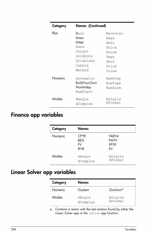
388 Variables
Finance app variables
Linear Solver app variables
Plot minmaxstepAxesCursorGridDotsGridLinesLabelsMethod
RecenterXmaxXminXtickXzoomYmaxYminYtickYzoom
Numeric AutomaticBuildYourOwnNumIndepNumStart
NumStepNumTypeNumZoom
Modes AAngleAComplex
ADigitsAFormat
Category Names (Continued)
Category Names
Numeric CPYRBEGFVIPYR
NbPmtPMTVPPYRPV
Modes AAngleAComplex
ADigitsAFormat
Category Names
Numeric LSystem LSolutiona
Modes AAngleAComplex
ADigitsAFormat
a. Contains a vector with the last solution found by either the Linear Solver app or the LSolve app function.
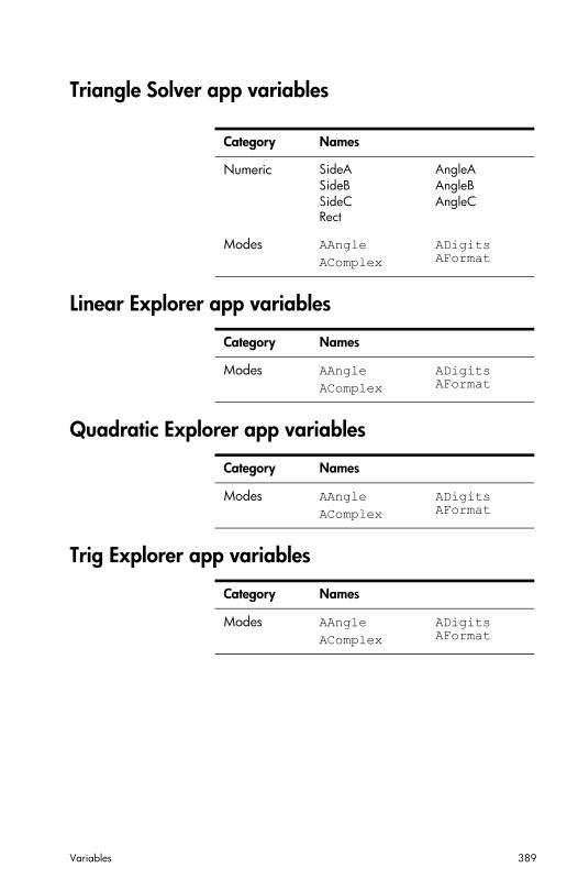
Variables 389
Triangle Solver app variables
Linear Explorer app variables
Quadratic Explorer app variables
Trig Explorer app variables
Category Names
Numeric SideASideBSideCRect
AngleAAngleBAngleC
Modes AAngleAComplex
ADigitsAFormat
Category Names
Modes AAngleAComplex
ADigitsAFormat
Category Names
Modes AAngleAComplex
ADigitsAFormat
Category Names
Modes AAngleAComplex
ADigitsAFormat

390 Variables
Sequence app variables
Category Names
Symbolic U1U2U3U4U5
U6U7U8U9U0
Plot AxesCursorGridDotsGridLinesLabelsNminNmaxRecenter
XmaxXminXtickXzoomYmaxYminYtickYzoom
Numeric AutomaticBuildYourOwnNumIndepNumStart
NumStepNumTypeNumZoom
Modes AAngleAComplex
ADigitsAFormat

Units and constants 391
22
Units and constants
UnitsA unit of measurement—such as inch, ohm, or Becquerel—enables you give a precise magnitude to a physical quantity.
You can attach a unit of measurement to any number or numerical result. A numerical value with units attached is referred to as a measurement. You can operate on measurements just as you do on numbers without attached units. The units are kept with the numbers in subsequent operations.
The units are on the Units menu. Press SF (Units) and, if necessary, tap .
The menu is organized by category. Each category is listed at the left, with the units in the selected category listed at the right.
Unit categories • length
• area
• volume
• time
• speed
• mass
• acceleration
• force
• energy
• power
• pressure
• temperature
• electricity
• light
• angle
• viscosity
• radiation

392 Units and constants
Prefixes The Units menu includes an entry that is not a unit category, namely, Prefix. Selecting this option displays a palette of prefixes.
Unit prefixes provide a handy way of entering large or small numbers. For example, the speed of light is approximately 300,000 m/s. If you wanted to use that in a calculation, you could enter it as 300_km/s, with the prefix k selected from the prefix palette.
Select the prefix you want before selecting the unit.
Unit calculationsA number plus a unit is a measurement. You can perform calculations with multiple measurements providing that the units of each measurement are from the same category. For example, you can add two measurements of length (even lengths of different units, as illustrated in the following example). But you cannot add, say, a length measurement to a volume measurement.
Example Suppose you want to add 20 centimeters and 5 inches and have the result displayed in centimeters.
Y: yotta Z: zetta E: exa P: peta T: tera
G: giga M: mega k: kilo h: hecto D: deca
d: deci c: centi m: milli : micro n: nano
p: pico f: femto a: atto z: zepto y: octo

Units and constants 393
1. If you want the result in cm, enter the centimeter measurement first.
20 SF (Units)
Select Length>Select cm
2. Now add 5 inches.
+ 5 SFSelect Length>
Select in
E
The result is shown as 32.7 cm. If you had wanted the result in inches, then you would have entered the 5 inches first.
3. To continue the example, let’s divide the result by 4 seconds.
n 4 SF
Select Time>Select s
E
The result is shown as 8.175 cm*s–1.

394 Units and constants
4. Now convert the result to kilometers per hour.
SFSelect CONVERT
Select 8.175_(cm/s) in History.
o1SFSelect Speed>Select km/h
E
The result is shown as 0.2943 kilometers per hour.
Unit toolsThere are a number of tools for managing and operating on units. These are available by pressing SFand tapping .
CONVERT Converts one unit to another unit of the same category.
CONVERT(5_m,1_ft) returns 16.4041994751_ft
You can also use the last answer as the first argument in a new conversion calculation. Pressing S+ places the last answer on the entry line. You can also select a value from history and tap to copy it to the entry line.
MKSA Meters, kilograms, seconds, amperes. Converts a complex unit into the base components of the MKSA system.
MKSA(8.175_cm/s) returns .08175_m*s–1
UFACTOR Unit factor conversion. Converts a measurement using a compound unit into a measurement expressed in constituent units. For example, a Coulomb—a measure of electric charge—is a compound unit derived from the SI base units of Ampere and second: 1 C = 1 A * 1 s. Thus:
UFACTOR(100_C,1_A)) returns 100 A*s

Units and constants 395
USIMPLIFY Unit simplification. For example, a Joule is defined as one kg*m2/s2. Thus:
USIMPLIFY(5_kg*m2/s2) returns 5_J
Physical constantsThe values of 34 math and physical constants can be selected by name and used in calculations. These constants are grouped into four categories: math, chemistry, physics and quantum mechanics. A list of all these constants is given in “List of constants” on page 396.
To display the constants, press SF and then tap
:
Example Suppose you want to know the potential energy of a mass of 5 units according to the equation E = mc2.
1. Enter the mass and the multiplication operator:
5 s
2. Open the constants menu.
SF
3. Select Physics.
4. Select c: 299792458.

396 Units and constants
5. Square the speed of light and evaluate the expression.
jE
Value or measurement?
You can enter just the value of a constant or the constant and its units (if it has units). If is showing on the screen, the value is inserted at the cursor point. If is showing on the screen, the value and its units are inserted at the cursor point.
In the example at the right, the first entry shows the Universal Gas Constant after it was chosen with showing. The second entry shows the same constant, but chosen when was showing.
Tapping displays , and vice versa.
List of constants
Category Name and symbol
Math eMAXREALMINREALi
Chemistry Avogadro NABoltmann, kmolar volume, Vmuniversal gas, Rstandard temperature, StdTstandard pressure, StdP

Units and constants 397
Phyics Stefan-Boltzmann, speed of light, cpermittivity, 0)permeability, 0acceleration of gravity, ggravitation, G
Quantum Planck, hDirac, electronic charge, qelectron mass, meq/me ratio, qmeproton mass, mpmp/me ratio, mpmefine structure, magnetic flux, Faraday, FRydberg, R∞Bohr radius, a0
Bohr magneton, B
nuclear magneton, N
photon wavelength, 0photon frequency, f0Compton wavelength, c
Category Name and symbol (Continued)

398 Units and constants

Lists 399
23
Lists
A list consists of comma-separated real or complex numbers, expressions, or matrices, all enclosed in braces. A list may, for example, contain a sequence of real numbers such as {1,2,3}. Lists represent a convenient way to group related objects.
You can do list operations in Home and in programs.
There are ten list variables available, named L0 to L9. You can use them in calculations or expressions in Home or in a program. Retrieve a list name from the Vars menu (a), or just type its name from the keyboard.
You can create, edit, delete, send, and receive named lists in the List Catalog: Sp(List). You can also create and store lists—named or unnnamed—in Home view.
List variables are identical in behavior to the columns C1-C0 in the Statistics 2Var app and the columns D1-D0 in the Statistics 1Var app. You can store a statistics column as a list (or vice versa) and use any of the list functions on the statistics columns, or the statistics functions on the list variables.
Create a list in the List Catalog1. Open the List
Catalog.
Sp(List)
The number of elements in a list is shown beside the list name.

400 Lists
2. Tap on the name you want to assign to the new list (L1, L2, etc.). The list editor appears.
If you’re creating a new list rather than changing, make sure you choose a list with out any elements in it.
3. Enter the values you want in the list, pressingE after each one.
Values can be real or complex numbers (or an expression). If you enter a expression, it is evaluated and the result is inserted in the list.
4. When done, press Sp(List) to return to the List catalog, or press Hto go to Home view.
List Catalog: Buttons and keys
The buttons and keys in the List Catalog are:
Button or Key Purpose
Opens the highlighted list for editing. You can also just tap on a list name.
or C Deletes the contents of the selected list.
Transmits the highlighted list to another HP Prime.
SJ(Clear) Clears all lists.
S=or \ Moves to the end or the beginning of the catalog.
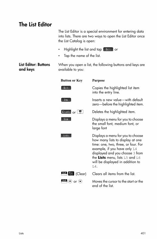
Lists 401
The List EditorThe List Editor is a special environment for entering data into lists. There are two ways to open the List Editor once the List Catalog is open:
• Highlight the list and tap or
• Tap the name of the list.
List Editor: Buttons and keys
When you open a list, the following buttons and keys are available to you:
Button or Key Purpose
Copies the highlighted list item into the entry line.
Inserts a new value—with default zero—before the highlighted item.
or C Deletes the highlighted item.
Displays a menu for you to choose the small font, medium font, or large font
Displays a menu for you to choose how many lists to display at one time: one, two, three, or four. For example, if you have only L4 displayed and you choose 3 from the Lists menu, lists L5 and L6 will be displayed in addition to L4.
SJ (Clear) Clears all items from the list.
S= or \ Moves the cursor to the start or the end of the list.

402 Lists
To edit a list 1. Open the List Catalog.
Sp(List)
2. Tap on the name of the list (L1, L1,etc.). The List Editor appears.
3. Tap on the element you want to edit. (Alternatively, press = or \ until the element you want to edit is highlighted.) In this example, edit the third element so that it has a value of 5.
5
To insert an element in a list
Suppose you want to insert a new value, 9, in L1(2) in the list L1 shown to the right.

Lists 403
Select L1(2), that is, the second element in the list.
9
Deleting listsTo delete a list In the List Catalog, use the cursor keys to highlight the list
and press C. You are prompted to confirm your decision. Tap or press E.
Only the contents of the list is deleted. The list is simply stripped of its contents.
To delete all lists In the List Catalog, pressSJ (Clear).
Only the contents of each list is deleted. The lists are simply stripped of their contents.
Lists in Home viewYou can enter and operate on lists directly in Home view. The lists can be named or unnamed.
To enter a list 1. Press Sq ({}).
A pair of braces appears on the entry line. All lists must be enclosed in braces.
2. Enter the first element in the list followed by a comma:
[element] o
3. Continue adding elements, separating each with a comma.
4. When you have finished entering the elements, press E. The list is added to History (with any expressions among the elements evaluated).

404 Lists
To store a list You can store a list in a variable. You can do this before the list is added to History, or you can copy it from History. When you’ve entered a list in the entry line or copied it from History to the entry line, tap
, enter a name for the list and press E. The list variable names available to you are L0 through L9.
For example, to store the list {25,147,8} in L7:
1. Create the list on the entry line.
2. Press > to move the cursor outside the list.
3. Tap .
4. Enter the name:
Aj7
5. Complete the operation: E.
To display a list To display a list in Home view, type its name and pressE.
If the list is empty, a pair of empty braces is returned.
To display one element
To display one element of a list in Home view, enter listname (element#). For example, if L6 is {3,4,5,6}, then L6(2)Ereturns 4.
To store one element
To store a value in one element of a list in Home view, enter value listname (element#). For example, to store 148 as the second element in L2, type148 L2(2)E.
To send a list You can send lists to another calculator or a PC just as you can apps, programs, matrices, and notes. See “Sharing data” on page 40 for instructions.

Lists 405
List functionsList functions are found on the Math menu. You can use them in Home and in programs.
You can type in the name of the function, or you can copy the name of the function from the List category of the Math menu.
Press D 6 to select the List category in the left column of the Math menu. (List is the sixth category on the Math menu, which is why pressing 6 will take you straight to the List category.) Press > to move to the sub-menu of list functions, select a function, and either tap or press E.
List functions are enclosed in parentheses. They have arguments that and separated by commas, as in CONCAT(L1,L2). An argument can be either a list variable name (such as L1) or the actual list. For example, REVERSE({1,2,3}).
Common operators like +, –, ×, and ÷ can take lists as arguments. If there are two arguments and both are lists, then the lists must have the same length, since the calculation pairs the elements. If there are two arguments and one is a real number, then the calculation operates on each element of the list.
Example:
5*{1,2,3} returns {5,10,15}.
Besides the common operators that can take numbers, matrices, or lists as arguments, there are commands that can only operate on lists.
Menu format By default, a List function is presented on the Math menu using its descriptive name, not its common command name. Thus the shorthand name CONCAT is presented as Concatenate and POS is presented as Position.

406 Lists
If you prefer the Math menu to show command names instead, deselect the Menu Display option on page 2 of the Home Settings screen (see page 26).
Make List Calculates a sequence of elements for a new list using the syntax:
MAKELIST(expression,variable,begin,end,increment)
Evaluates expression with respect to variable, as variable takes on values from begin to end values, taken at increment steps.
Example:
In Home, generate a series of squares from 23 to 27:
D 6 1A a j oA a o 23 o 27o1E
Sort Sorts the elements in a list in ascending order.
SORT(list)
Example:
SORT({2,5,3}) returns {2,3,5}
Reverse Creates a list by reversing the order of the elements in a list.
REVERSE(list)
Example:
REVERSE({1,2,3}) returns {3,2,1}
Concatenate Concatenates two lists into a new list.

Lists 407
CONCAT(list1, list2)
Example:
CONCAT({1,2,3},{4}) returns {1,2,3,4}.
Position Returns the position of an element within a list. The element can be a value, a variable, or an expression. If there is more than one instance of the element, the position of the first occurrence is returned. A value of 0 is returned if there is no occurrence of the specified element.
POS(list, element)
Example:
POS ({3,7,12,19},12) returns 3
Size Returns the number of elements in a list.
SIZE(list)
Example:
SIZE({1,2,3}) returns 3
LIST Creates a new list composed of the first differences, that is, the differences between consecutive elements in a list. The new list has one less element than the original list. The differences for {x1, x2, x3,... xn-1, xn} are {x2–x1, x3–x2 ,... xn–xn–1}.
LIST(list1)
Example:
In Home view, store {3,5,8,12,17,23} in L5 and find the first differences for the list.
Sq3,5,8,12,17,23> A j 5ED 6 7 A j 5 E

408 Lists
LIST Calculates the sum of all elements in a list.
LIST(list)
Example:
LIST({2,3,4}) returns 9.
LIST Calculates the product of all elements in list.
LIST(list)
Example:
LIST({2,3,4}) returns 24.
Finding statistical values for listsTo find statistical values—such as the mean, median, maximum, and minimum of a list—you create a list, store it in a data set and then use the Statistics 1Var app.
Example In this example, use the Statistics 1Var app to find the mean, median, maximum, and minimum values of the elements in the list L1, being 88, 90, 89, 65, 70, and 89.
1. In Home view, create L1.
S q 88, 90, 89, 65, 70,89 > Aj1E
2. In Home view, store L1 in D1.
Aj1 Ad1E
You will now be able to see the list data in the Numeric view of the Statistics 1Var app.

Lists 409
3. Start the Statistics 1Var app.
I Select Statistics 1Var
Notice that your list elements are in data set D1.
4. In the Symbolic view, specify the data set whose statistics you want to find.
Y
By default, H1 will use the data in D1, so nothing further needs to be done in Symbolic view. However, if the data of interest were in D2, or any column other than D1, you would have to specify the desired data column here.
5. Calculate the statistics.
M
6. Tap when you are done.
See the chapter 9, “Statistics 1Var app”, beginning on page 187, for the meaning of each statistic.

410 Lists
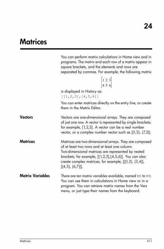
Matrices 411
24
Matrices
You can perform matrix calculations in Home view and in programs. The matrix and each row of a matrix appear in square brackets, and the elements and rows are separated by commas. For example, the following matrix:
is displayed in History as:[[1,2,3],[4,5,6]]
You can enter matrices directly on the entry line, or create them in the Matrix Editor.
Vectors Vectors are one-dimensional arrays. They are composed of just one row. A vector is represented by single brackets; for example, [1,2,3]. A vector can be a real number vector, or a complex number vector such as [(1,2), (7,3)].
Matrices Matrices are two-dimensional arrays. They are composed of at least two rows and at least one column. Two-dimensional matrices are represented by nested brackets; for example, [[1,2,3],[4,5,6]]. You can also create complex matrices, for example, [[(1,2), (3,4)], [(4,5), (6,7)]].
Matrix Variables There are ten matrix variables available, named M0 to M9. You can use them in calculations in Home view or in a program. You can retrieve matrix names from the Vars menu, or just type their names from the keyboard.
1 2 3
4 5 6

412 Matrices
Creating and storing matricesThe Matrix Catalog contains the matrix variables M0-M9. Once you select a matrix name, you can create, edit, and delete matrices in the Matrix Editor. You can also send a matrix to another HP Prime.
To open the Matrix Catalog, pressSt(Matrix).
In the Matrix Catalog, the size of a matrix is shown beside the matrix name. (An empty matrix is shown as 1*1.) The number of elements in it is shown beside a vector.
You can also create and store matrices—named or unnamed—in Home view. For example, the command:
POLYROOT([1,0,–1,0])M1
stores the roots of the complex vector of length 3 into the variable M1. M1 will thus contain the three roots of
: 0, 1 and –1.
Matrix Catalog: buttons and keys
The buttons and keys available in the Matrix Catalog are:
x3 x– 0=
Button or Key Purpose
Opens the highlighted matrix for editing.
or C Deletes the content sof the selected matrix.
Changes the selected matrix into a one-dimensional vector.
Transmits the highlighted matrix to another HP Prime.
SJ(Clear) Clears the contents of all matrices.

Matrices 413
Working with matricesTo open the Matrix Editor
To create or edit a matrix, go to the Matrix Catalog, and tap on a matrix. (You could also use the cursor keys to highlight the matrix and then press .) The Matrix Editor opens.
Matrix Editor: Buttons and keys
The buttons and keys available in the Matrix Editor are.:
Button or Key Purpose
Copies the highlighted element to the entry line.
Inserts a row of zeros above, or a column of zeros to the left, of the highlighted cell. You are prompted to choose row or column.
Displays a menu for you to choose the small font, medium font, or large font.
A three-way toggle that controls how the cursor will move after an element has been entered. moves the cursor to the right,
moves it downward, and does not move it at all.
Displays a menu for you to choose 1, 2, 3, or 4 columns to be displayed at a time.
C Replaces the contents of the highlighted cell with a zero.
SJ(Clear) Deletes the highlighted row, or column, or the entire matrix. (You are prompted to make a choice.)
S=\<> Moves the cursor to the first row, last row, first column, or last column respectively.
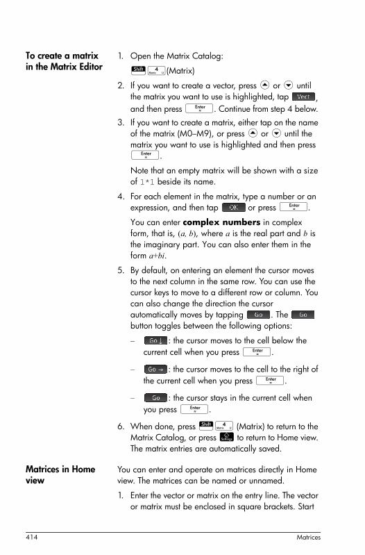
414 Matrices
To create a matrix in the Matrix Editor
1. Open the Matrix Catalog:
St(Matrix)
2. If you want to create a vector, press = or \ until the matrix you want to use is highlighted, tap , and then press E. Continue from step 4 below.
3. If you want to create a matrix, either tap on the name of the matrix (M0–M9), or press = or \ until the matrix you want to use is highlighted and then press E.
Note that an empty matrix will be shown with a size of 1*1 beside its name.
4. For each element in the matrix, type a number or an expression, and then tap or press E.
You can enter complex numbers in complex form, that is, (a, b), where a is the real part and b is the imaginary part. You can also enter them in the form a+bi.
5. By default, on entering an element the cursor moves to the next column in the same row. You can use the cursor keys to move to a different row or column. You can also change the direction the cursor automatically moves by tapping . The button toggles between the following options:
– : the cursor moves to the cell below the current cell when you press E.
– : the cursor moves to the cell to the right of the current cell when you press E.
– : the cursor stays in the current cell when you press E.
6. When done, press St (Matrix) to return to the Matrix Catalog, or press H to return to Home view. The matrix entries are automatically saved.
Matrices in Home view
You can enter and operate on matrices directly in Home view. The matrices can be named or unnamed.
1. Enter the vector or matrix on the entry line. The vector or matrix must be enclosed in square brackets. Start

Matrices 415
each row of a matrix with square brackets as well. (For a pair of square brackets, press Su.)
Separate each element and each row with a comma (o).
2. When you have finished entering the elements, press E. The vector or matrix is added to History (with any expressions among the elements evaluated).
3. Press Eto evaluate and display the vector or matrix.
To store a matrix You can store it a vector or matrix in a variable. You can do this before it is added to History, or you can copy it from History. When you’ve entered a vector or matrix in the entry line or copied it from History to the entry line, tap
, enter a name for it and press E. The vector and matrix names variable names available to you are M0 through M9.
The screen at the left shows the matrix [[2.5,729],[16,2]] being stored in M5. Note that you can enter an expression (like 5/2) for an element of the matrix, and it will be evaluated.
The screen at the right shows the vector [66,33,11] being stored in M6.
To display a matrix In Home view, enter the name of the vector or matrix and press E. If the vector or matrix is empty, zero is returned inside double square brackets.

416 Matrices
To display one element
In Home view, enter matrixname(row,column). For example, if M2 is [[3,4],[5,6]], then M2(1,2)Ereturns 4.
To store one element
In Home view, enter value, tap , and then enter matrixname(row,column).For example, to change the element in the first row and second column of M5 to 728 and then display the resulting matrix:
728 AQ5
R1o 2 E
An attempt to store an element to a row or column beyond the size of the matrix results in re-sizing the matrix to allow the storage. Any intermediate cells will be filled with zeroes.
To send a matrix You can send matrices between calculators just as you can send apps, programs, lists, and notes. See “Sharing data” on page 40 for instructions.
Matrix arithmeticYou can use the arithmetic functions (+, –, ×, ÷, and powers) with matrix arguments. Division left-multiplies by the inverse of the divisor. You can enter the matrices themselves or enter the names of stored matrix variables. The matrices can be real or complex.
For the next examples, store [[1,2],[3,4]] in M1 and [[5,6],[7,8]] in M2.
Example 1. Select the first matrix:
St (Matrix)Tap M1 or highlight it and press E.

Matrices 417
2. Enter the matrix elements:
1 E 2 E 3 E 4 E
3. Select the second matrix:
St (Matrix)Tap M2 or highlight it and press E.
4. Enter the matrix elements:
5 E 6 E 7 E 8 E
5. In Home view, add the two matrices you have just created.
HA Q1 + A Q2 E
To multiply and divide by a scalar
For division by a scalar, enter the matrix first, then the operator, then the scalar. For multiplication, the order of the operands does not matter.
The matrix and the scalar can be real or complex. For example, to divide the result of the previous example by 2, press the following keys:
n 2 E
To multiply two matrices
To multiply the two matrices that you created for the previous example, press the following keys:

418 Matrices
AQ1sAQ2E
To multiply a matrix by a vector, enter the matrix first, then the vector. The number of elements in the vector must equal the number of columns in the matrix.
To raise a matrix to a power
You can raise a matrix to any power as long as the power is an integer. The following example shows the result of raising matrix M1, created earlier, to the power of 5.
AQ1k5E
You can also raise a matrix to a power without first storing it as a variable.
Matrices can also be raised to negative powers. In this case, the result is equivalent to 1/[matrix]^ABS(power). In the following example, M1 is raised to the power of –2.
AQ1kQ
2E
To divide by a square matrix
For division of a matrix or a vector by a square matrix, the number of rows of the dividend (or the number of elements, if it is a vector) must equal the number of rows in the divisor.
This operation is not a mathematical division: it is a left- multiplication by the inverse of the divisor. M1/M2 is equivalent to M2–1 * M1.

Matrices 419
To divide the two matrices you created for the previous example, press the following keys:
A Q1 n A Q2
To invert a matrix You can invert a square matrix in Home view by typing the matrix (or its variable name) and pressing SnE. You can also use the INVERSE command in the Matrix category of the Math menu.
To negate each element
You can change the sign of each element in a matrix by pressing Q, entering the matrix name, and pressing E.
Solving systems of linear equations
You can use matrices to solve systems of linear equations, such as the following:
2x+3y+4z=5x+y–z=7
4x–y+2z=1
In this example we will use matrices M1 and M2, but you could use any of the ten matrices available.
1. Open the Matrix Catalog, clear M1, choose to create a vector, and open the Matrix Editor:
St [select M1] C
E

420 Matrices
2. Create the vector of the three constants in the linear system.
5E7E1E
3. Return to the Matrix Catalog.
St
The size of M1 should be showing as 3.
4. Select and clear M2, and re-open the Matrix Editor:
[Press \ or = to select M2] C
E5. Enter the equation
coefficients.2E3E[Tap in cell R1, C3.] 4E 1E1EQ1E4EQ1E2E
6. Return to Home view and left-multiply the constants vector by the inverse of the coefficients matrix:
HA Q2S ns A Q1E
The result is a vector of the solutions: x = 2, y = 3 and z = –2.

Matrices 421
An alternative method is to use the RREF function (see page 422).
Matrix functions and commandsFunctions • Functions can be used in any app or in Home view.
They are listed on the Math menu under the Matrix category. They can be used in mathematical expressions—primarily in Home view—as well as in programs.
• Functions always produce and display a result. They do not change any stored variables, such as a matrix variable.
• Functions have arguments that are enclosed in parentheses and separated by commas; for example, CROSS(vector1,vector2). The matrix input can be either a matrix variable name (such as M1) or the actual matrix data inside brackets. For example, CROSS(M1,[1,2]).
Menu format By default, a Matrix function is presented on the Math menu using its descriptive name, not its common command name. Thus the shorthand name TRN is presented as Transpose and DET is presented as Determinant.
If you prefer the Math menu to show command names instead, deselect the Menu Display option on page 2 of the Home Settings screen (see page 26).
Commands Functions differ from commands in that a function can be used in an expression. Commands cannot be used in an expression.
Matrix commands are listed among the functions and commands in the commands catalog, one of the Toolbox menus. Press D and tap to display the commands catalog.
Argument conventions
• For row# or column#, supply the number of the row (counting from the top, starting with 1) or the number of the column (counting from the left, starting with 1).
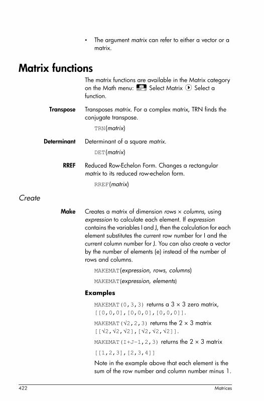
422 Matrices
• The argument matrix can refer to either a vector or a matrix.
Matrix functionsThe matrix functions are available in the Matrix category on the Math menu: D Select Matrix > Select a function.
Transpose Transposes matrix. For a complex matrix, TRN finds the conjugate transpose.
TRN(matrix)
Determinant Determinant of a square matrix.
DET(matrix)
RREF Reduced Row-Echelon Form. Changes a rectangular matrix to its reduced row-echelon form.
RREF(matrix)
Create
Make Creates a matrix of dimension rows × columns, using expression to calculate each element. If expression contains the variables I and J, then the calculation for each element substitutes the current row number for I and the current column number for J. You can also create a vector by the number of elements (e) instead of the number of rows and columns.
MAKEMAT (expression, rows, columns)
MAKEMAT (expression, elements)
Examples
MAKEMAT(0,3,3) returns a 3 × 3 zero matrix, [[0,0,0],[0,0,0],[0,0,0]].
MAKEMAT(√2,2,3) returns the 2 × 3 matrix [[√2,√2,√2],[√2,√2,√2]].
MAKEMAT(I+J–1,2,3) returns the 2 × 3 matrix
[[1,2,3],[2,3,4]]
Note in the example above that each element is the sum of the row number and column number minus 1.

Matrices 423
MAKEMAT(√2,2) returns the 2-element vector [√2,√2].
Identity Identity matrix. Creates a square matrix of dimensionsize × size whose diagonal elements are 1 and off-diagonal elements are zero.
IDENMAT(size)
Random Returns a list of size n or a n x m matrix that contains random integers in the range −99 through 99 with uniform distribution or that contains random numbers according to the law put between quote.
randMat(Intg(n), [Intg(m)],[Interval or quote(DistribLaw)])
JordanBlock Returns a matrix n x n with a on the diagonal, 1 above and 0 everywhere else.
JordanBlock(Expr(a),Intg(n))
Hilbert Returns the order n Hilbert matrix: Hjk=1/(j+k+1) j,k=1...n.
hilbert(Intg(n))
Isometric Matrix of an isometry given by its proper elements.
mkisom(Vect,(Sign(1) or -1))
Vandermonde Returns the Vandermonde matrix=[V^0,V^1,...].
vandermonde(Vect(V))
Basic
Norm Finds the norm of a matrix.
ABS(matrix)
Row Norm Row Norm. Finds the maximum value (over all rows) for the sums of the absolute values of all elements in a row.
ROWNORM(matrix)
Column Norm Column Norm. Finds the maximum value (over all columns) of the sums of the absolute values of all elements in a column.
COLNORM(matrix)

424 Matrices
Spectral Norm Spectral Norm of matrix.
SPECNORM (matrix)
Spectral Radius Spectral Radius of a square matrix.
SPECRAD (matrix)
Condition Condition Number. Finds the 1-norm (column norm) of a square matrix.
COND(matrix)
Rank Rank of a rectangular matrix.
RANK(matrix)
Pivot Performs one step of the Gauss-Jordan reduction method on an n x m matrix A using the element A[nl,nc] (0≤nl≤n and 0≤nc≤m) as pivot, and returns an equivalent matrix with zeros in all elements in column nc except that in row nl.
pivot(Mtrx(A),Intg(nl),Intg(nc))
Trace Finds the trace of a square matrix. The trace is equal to the sum of the diagonal elements. (It is also equal to the sum of the eigenvalues.)
TRACE(matrix)
Advanced
Eigenvalues Displays the eigenvalues in vector form for matrix.
EIGENVAL (matrix)
Eigenvectors Eigenvectors and eigenvalues for a square matrix. Displays a list of two arrays. The first contains the eigenvectors and the second contains the eigenvalues.
EIGENVV (matrix)
Jordan Returns the list made by the matrix of passage and the Jordan form of a matrix.
jordan(Mtrx)
Diagonal Returns either the diagonal matrix with diagonal l or the diagonal of A.
diag(Lst(l)||Mtrx(A))

Matrices 425
Cholesky For a numerical symmetric matrix A, returns L matrix such that A=L*tran(L).
cholesky(Mtrx)
Hermite Hermite normal form of a matrix with coefficients in Z: returns U,B such that U is invertible in Z, B is upper triangular and B=U*A.
ihermite(Mtrx(A))
Hessenberg Matrix reduction to Hessenberg form. Returns [P,B] such that B=inv(P)*A*P.
hessenberg(Mtrx(A))
Smith Smith normal form of a matrix with coefficients in Z: returns U,B,V such that U and V invertible in Z, B is diagonal, B[i,i] divides B[i+1,i+1], and B=U*A*V.
ismith(Mtrx(A))
Factorize
LQ LQ Factorization. Factorizes a m × n matrix into three matrices L, Q, and P, where {[L[m × n lowertrapezoidal]],[Q[n × n orthogonal]],[P[m × m permutation]]}and P*A=L*Q.
LQ(matrix)
LSQ Least Squares. Displays the minimum norm least squares matrix (or vector) corresponding to the system matrix1*X=matrix2.
LSQ(matrix1, matrix2)
LU LU Decomposition. Factorizes a square matrix into three matrices L, U, and P, where {[L[lowertriangular]],[U[uppertriangular]],[P[permutation]]}}and P*A=L*U.
LU(matrix)
QR QR Factorization. Factorizes an m×n matrix A numerically as Q*R, where Q is an orthogonal matrix and R is an upper triangular matrix, and returns R. R is stored in var2 and Q=A*inv(R) is stored in var1.
QR(matrix A,var1,var2)

426 Matrices
SCHUR Schur Decomposition. Factorizes a square matrix into two matrices. If matrix is real, then the result is {[[orthogonal]],[[upper-quasi triangular]]}.If matrix is complex, then the result is {[[unitary]],[[upper-triangular]]}.
SCHUR(matrix)
SVD Singular Value Decomposition. Factorizes an m × n matrix into two matrices and a vector: {[[m × m square orthogonal]],[[n × n square orthogonal]], [real]}.
SVD(matrix)
SVL Singular Values. Returns a vector containing the singular values of matrix.
SVL(matrix)
Vector
Cross Product Cross Product of vector1 with vector2.
CROSS(vector1, vector2)
Dot Product Dot Product of two arrays, matrix1 and matrix2.
DOT(matrix1, matrix2)
L2 Norm Returns the l2 norm (sqrt(x1^2+x2^2+...xn^2)) of a vector.
l2norm(Vect)
L1 Norm Returns the l1 norm (sum of the absolute values of the coordinates) of a vector.
l1norm(Vect)
Max Norm Returns the l∞ norm (the maximum of the absolute values of the coordinates) of a vector.
maxnorm(Vect or Mtrx)
Examples
Identity Matrix You can create an identity matrix with the IDENMAT function. For example, IDENMAT(2) creates the 2×2 identity matrix [[1,0],[0,1]].

Matrices 427
You can also create an identity matrix using the MAKEMAT (make matrix) function. For example, entering MAKEMAT(I≠J,4,4) creates a 4 × 4 matrix showing the numeral 1 for all elements except zeros on the diagonal. The logical operator (≠) returns 0 when I (the row number) and J (the column number) are equal, and returns 1 when they are not equal. (You can insert ≠ by choosing it from the relations palette: Sv.)
Transposing a Matrix
The TRN function swaps the row–column and column–row elements of a matrix. For instance, element 1,2 (row 1, column 2) is swapped with element 2,1; element 2,3 is swapped with element 3,2; and so on.
For example, TRN([[1,2],[3,4]]) creates the matrix [[1,3],[2,4]].
Reduced-Row Echelon Form
The set of equations
can be written as the augmented matrix
which can then be stored as a real matrix in any matrix variable. M1 is used in this example.
You can then use the RREF function to change this to reduced-row echelon form, storing it in any matrix variable. M2 is used in this example.
x 2y– 3z+ 142x y z–+ 34x
–2y– 2z+ 14
==
=
1 2– 3 14
2 1 1– 3–
4 2– 2 14
3 4

428 Matrices
The reduced row echelon matrix gives the solution to the linear equation in the fourth column.
An advantage of using the RREF function is that it will also work with inconsistent matrices resulting from systems of equations which have no solution or infinite solutions.
For example, the following set of equations has an infinite number of solutions:
The final row of zeros in the reduced-row echelon form of the augmented matrix indicates an inconsistent system with infinite solutions.
x y z–+ 52x y– 7x 2y– z+ 2
==
=

Notes and Info 429
25
Notes and Info
The HP Prime has two text editors for entering notes:
• The Note Editor: opens from within the Note Catalog (which is a collection of notes independent of apps).
• The Info Editor: opens from the Info view of an app. A note created in the Info view is associated with the app and stays with it if you send the app to another calculator.
The Note CatalogSubject to available memory, you can store as many notes as you want in the Note Catalog. These notes are independent of any app. The Note Catalog lists the notes by name. This list excludes notes that were created in any app’s Info view, but these can be copied and then pasted into the Note Catalog via the clipboard. From the Note Catalog, you create or edit individual notes in the Note Editor.
Note Catalog: button and keys
While you are in the Note Catalog, you can use the following buttons and keys. Note that some buttons will not be available if there are no notes in the Note Catalog.
Button or Key Purpose
Opens the selected note for editing.
Begins a new note, and prompts you for a name.
Tap to provide additional features. See below.

430 Notes and Info
The Note EditorThe Note Editor is where you create and edit notes. You can launch the Note Editor from the Notes Catalog, and also from within an app. Notes created within an app stay with that app even if you send the app to another calculator. Such notes do not appear in the Notes Catalog. They can only be read when the associated app is open. Notes created via the Notes Catalog are not specific to any app and can be viewed at any time by opening the Notes Catalog. Such notes can also be sent to another calculator.
To create a note from the Notes Catalog
1. Open the Note Catalog.
SN
Save creates a copy of the selected note and prompts you to save it under a new name.
Rename renames the selected note.
Sort sorts the list of notes (sort options are alphabetical and chronological).
Delete deletes the selected note.
Clear deletes all notes.
C Deletes the selected note.
SJ Deletes all notes in the catalog.
Sends the selected note to another HP Prime or PC.
Button or Key Purpose (Continued)

Notes and Info 431
2. Create a new note.
3. Enter a name for your note. In this example, we’ll call the note MYNOTE.
AA MYNOTE
4. Write your note, using the editing keys and formatting options described in the following sections.
When you are finished, exit the Note Editor by pressing H or pressing I and opening an app. Your work is automatically saved. To access your new note, return to the Notes Catalog.
To create a note for an app
You can also create a note that is specific to an app and which stays with the app should you send the app to another calculator. See “Adding a note to an app” on page 96. Notes created this way take advantage of all the formatting features of the Note Editor (see below).
Note Editor: buttons and keys
The following buttons and keys are available while you are adding or editing a note.
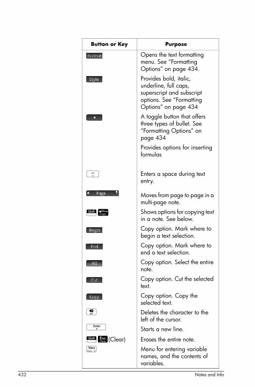
432 Notes and Info
Button or Key Purpose
Opens the text formatting menu. See “Formatting Options” on page 434.
Provides bold, italic, underline, full caps, superscript and subscript options. See “Formatting Options” on page 434
A toggle button that offers three types of bullet. See “Formatting Options” on page 434
Provides options for inserting formulas
X Enters a space during text entry.
Moves from page to page in a multi-page note.
SV Shows options for copying text in a note. See below.
Copy option. Mark where to begin a text selection.
Copy option. Mark where to end a text selection.
Copy option. Select the entire note.
Copy option. Cut the selected text.
Copy option. Copy the selected text.
C Deletes the character to the left of the cursor.
E Starts a new line.
SJ(Clear) Erases the entire note.
a Menu for entering variable names, and the contents of variables.

Notes and Info 433
Entering uppercase and lowercase characters The following table below describes how to quickly enter uppercase and lowercase characters.
D Menu for entering math commands.
Sa (Chars) Displays a palette of special characters. To type one, highlight it and tap or press E. To copy a character without closing the Chars menu, select it and tap
.
Button or Key Purpose (Continued)
Purpose Keys
Make the next character upper-case A
Lock mode: make all characters uppercase until the mode is reset
AA
With uppercase locked, make next character lowercase
S
With uppercase locked, make all characters lowercase until the mode is reset
SA
Reset uppercase lock mode A
Make the next character lower-case AS
Lock mode: make all characters lowercase until the mode is reset
ASA
With lowercase locked, make next character uppercase
S
With lowercase locked, make all characters uppercase until the mode is reset
SA
Reset lowercase lock mode AAA
A

434 Notes and Info
The left side of the notification area of the title bar will indicate what case will be applied to the character you next enter.
Text formatting You can enter text in different formats in the Note Editor. Choose a formatting option before you start entering text. The formatting options are described in “Formatting Options” below.
Formatting OptionsFormatting options are available from three touch buttons in the Note Editor and in the Info view of an app:
The formatting options are listed in the table below.
Category Options
Font Size• 10–22 pt
Foreground ColorSelect from twenty colors.
Background ColorSelect from twenty colors.
Align(text alignment)
• Left• Center• Right
Font Style• Bold• Italic• Underline• Strikethrough• Superscript• Subscript
Bullets• •
• ◦•• [Cancels bullet]
Δ

Notes and Info 435
To import a note You can import a note from the Note Catalog into an app's Info view and vice versa.
Suppose you want to copy a note named Assignments from the Note Catalog into the Function Info view:
1. Open the Note Catalog.
SN
2. Select the note Assignments and tap
3. Open the copy options for copying to the clipboard.
SV (Copy))
The menu buttons change to give you options for copying:
: Marks where the copying or cutting is to begin.
: Marks where the copying or cutting is to end.
: Select the entire program.
: Cut the selection.
: Copy the selection.4. Select what you want to copy or cut (using the options
listed immediately above).
5. Tap or .
6. Open the Info view of the Function app.
I, tap the Function app icon, press SI.7. Move the cursor to the location where you want the
copied text to be pasted and open the clipboard.
SZ
8. Select the text from the clipboard and press .
Sharing notes You can send a note to another HP Prime. See “Sharing data” on page 40.

436 Notes and Info

Programming 437
26
Programming
This chapter describes how to program the HP Prime. In this chapter you’ll learn about:
• programming commands
• writing functions in programs
• using variables in programs
• executing programs
• debugging programs
• creating programs for building custom apps
• sending a program to another HP Prime
HP Prime Programs
An HP Prime program contains a sequence of commands that execute automatically to perform a task.
Command Structure
Commands are separated by a semicolon ( ; ). Commands that take multiple arguments have those arguments enclosed in parentheses and separated by a comma( , ). For example,
PIXON (xposition, yposition);
Sometimes, arguments to a command are optional. If an argument is omitted, a default value is used in its place. In the case of the PIXON command, a third argument could be used that specifies the color of the pixel:
PIXON (xposition, yposition [,color]);
The last argument indicates which of four colors to use when lighting up the pixel. Here, the default value is 0 (black). In this manual, optional arguments to commands appear inside square brackets, as shown above. In the PIXON example, a graphics variable (G) could be specified as the first argument. The default is G0, which always contains the currently displayed screen. Thus, the full syntax for the PIXON command is:

438 Programming
PIXON([G,] xposition, yposition [ ,color]);
Some built-in commands employ an alternative syntax whereby function arguments do not appear in parentheses. Examples include RETURN and RANDOM.
Program Structure
Programs can contain any number of subroutines (each of which is a function or procedure). Subroutines start with a heading consisting of the name, followed by parentheses that contain a list of parameters or arguments, separated by commas. The body of a subroutine is a sequence of statements enclosed within a BEGIN–END; pair. For example, the body of a simple program, called MYPROGRAM, could look like this:
EXPORT MYPROGAM()
BEGIN
PIXON(1,1);
END;
Comments When a line of a program begins with two forward slashes, //, the rest of the line will be ignored. This enables you to insert comments in the program:
EXPORT MYPROGAM()
BEGIN
PIXON(1,1);
//This line is just a comment.
END;
The Program CatalogThe Program Catalog is where you run and debug programs, and send programs to another HP Prime. You can also rename and remove programs, and it is where you start the Program Editor. The Program Editor is where you create and edit programs. Programs can also be run from Home view or from other programs.
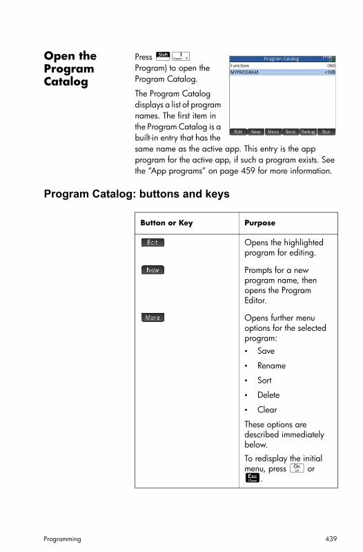
Programming 439
Open the Program Catalog
Press Sx Program) to open the Program Catalog.
The Program Catalog displays a list of program names. The first item in the Program Catalog is a built-in entry that has the same name as the active app. This entry is the app program for the active app, if such a program exists. See the “App programs” on page 459 for more information.
Program Catalog: buttons and keys
Button or Key Purpose
Opens the highlighted program for editing.
Prompts for a new program name, then opens the Program Editor.
Opens further menu options for the selected program:• Save
• Rename
• Sort
• Delete
• Clear
These options are described immediately below.
To redisplay the initial menu, press O or J.

440 Programming
Save creates a copy of the selected program with a new name you are prompted to give.
Rename renames the selected program.
Sort sorts the list of programs. (Sort options are alphabetical and chronological).
Delete deletes the selected program.
Clear deletes all programs.
Transmits the highlighted program to another HP Prime or to a PC.
Debugs the selectedprogram.
Runs the highlighted program.
S= or S\ Moves to the beginning or end of the Program Catalog.
C Deletes the selected program.
SJ Deletes all programs.
Button or Key Purpose (Continued)
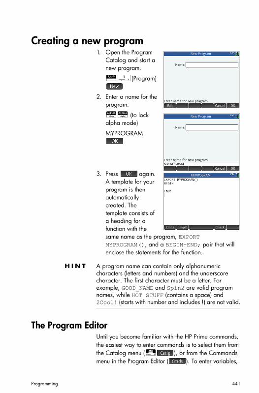
Programming 441
Creating a new program1. Open the Program
Catalog and start a new program.
Sx (Program)
2. Enter a name for the program.
AA (to lock alpha mode)
MYPROGRAM .
3. Press again. A template for your program is then automatically created. The template consists of a heading for a function with the same name as the program, EXPORT MYPROGRAM(), and a BEGIN–END; pair that will enclose the statements for the function.
H I N T A program name can contain only alphanumeric characters (letters and numbers) and the underscore character. The first character must be a letter. For example, GOOD_NAME and Spin2 are valid program names, while HOT STUFF (contains a space) and 2Cool! (starts with number and includes !) are not valid.
The Program EditorUntil you become familiar with the HP Prime commands, the easiest way to enter commands is to select them from the Catalog menu (D ), or from the Commands menu in the Program Editor ( ). To enter variables,

442 Programming
symbols, mathematical functions, units, or characters, use the keyboard keys.
Program Editor: buttons and keys
The buttons and keys in the Program Editor are:Entering a program
Button or Key Meaning
Checks the current program for errors.
or
S= and S\
If your programs goes beyond one screen, you can quickly jump from screen to screen by tapping either side of this button. Tap the left side of the button to display the previous page; tap the right side to display the next page. (The left tap will be inactive if you have the first page of the program displayed.)
Opens a menu from which you can choose from common programming commands. The commands are grouped under the options:• Strings
• Drawing
• Matrix
• App Functions
• Integer
• I/O
• More
Press J to return to the main menu.The commands in this menu are described in “Commands under the Cmds menu”, beginning on page 470.

Programming 443
Opens a menu from which you can select common programming commands. The commands are grouped under the options:• Block
• Branch
• Loop
• Variable
• Function
Press J to return to the main menu.
The commands in this menu are described in “Commands under the Tmplt menu”, beginning on page 465.
a Displays menus for selecting variable names and values.
Sa(Chars)
Displays a palette of characters. If you display this palette while a program is open, you can choose a character and it will be be added to your program at the cursor point. To add one character, highlight it and tap
or press E. To add a character without closing the characters palette, select it and tap .
S> and S<
Moves the cursor to the end (or beginning) of the current line.
E Starts a new line.
C Deletes the character to the left of the cursor.
Button or Key Meaning (Continued)
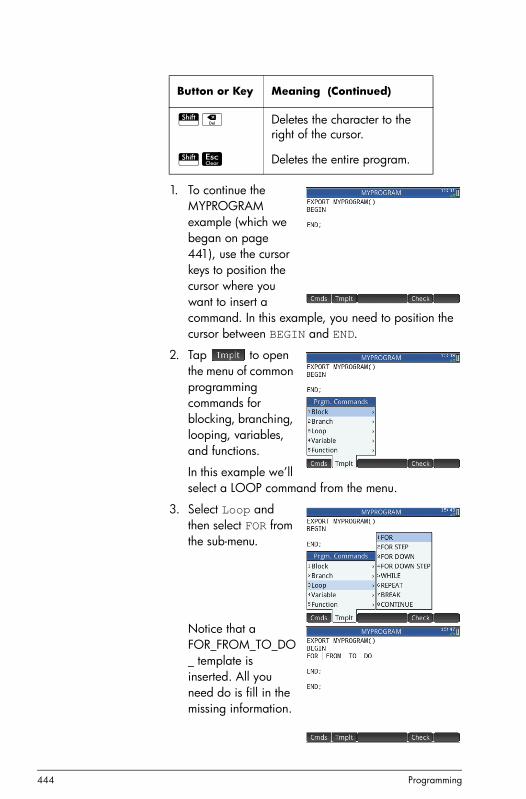
444 Programming
1. To continue the MYPROGRAM example (which we began on page 441), use the cursor keys to position the cursor where you want to insert a command. In this example, you need to position the cursor between BEGIN and END.
2. Tap to open the menu of common programming commands for blocking, branching, looping, variables, and functions.
In this example we’ll select a LOOP command from the menu.
3. Select Loop and then select FOR from the sub-menu.
Notice that a FOR_FROM_TO_DO_ template is inserted. All you need do is fill in the missing information.
SC Deletes the character to the right of the cursor.
SJ Deletes the entire program.
Button or Key Meaning (Continued)

Programming 445
4. Using the cursor keys and keyboard, fill in the missing parts of the command. In this case, make the statement match the following:
FOR N FROM 1 TO 3 DO
5. Move the cursor to a blank line below the FOR statement.
6. Tap to open the menu of common programming commands.
7. Select I/O and then select MSGBOX from the sub-menu.
8. Fill in the argument of the MSGBOX command, and type a semicolon at the end of the command.
9. Tap to check the syntax of your program.
10.When you are finished, press Sx to return to the Program Catalog or H to go to Home view. You are ready now to execute the program.
Run a Program
From Home view, enter the name of the program, with a pair of parentheses after it. If the program takes any arguments, insert these in the parentheses, separated by commas. To run the program, press E.
From the Program Catalog, highlight the program you want to run and tap . When a program is executed from the catalog, the system looks for a function named

446 Programming
START() (no parameters). If it finds one, that function is run. Otherwise, it looks for a function with the same name as the program. If the system finds one, it runs it. Otherwise, nothing happens.
You can also run a program from the USER menu (one of the Toolbox menus):
D
Tap MYPROGRAM and MYPROGRAM appears on the entry line. Tap E and the program executes, displaying a message box.
Tap three times to step through the FOR loop. Notice that the number shown increments by 1 each time.
After the program terminates, you can resume any other activity with the HP Prime.
If a program has arguments, when you press a screen appears prompting you to enter the program parameters.
What you see will differ slightly depending on where you started the program. If you start the program from the Home view, the HP Prime displays the contents of Ans (Home variable containing the last result) when the program has finished. If you start the program from the Program Catalog by tapping the button, the HP Prime returns you to the Program Catalog when the program ends.
Multi-function programs
If there is more than one EXPORT function in a program, when is tapped a list appears for you to choose which function to run. To see this feature, create a program with the text:
EXPORT NAME1( )
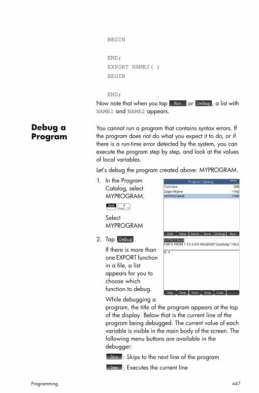
Programming 447
BEGIN
END;
EXPORT NAME2( )
BEGIN
END;
Now note that when you tap or , a list with NAME1 and NAME2 appears.
Debug a Program
You cannot run a program that contains syntax errors. If the program does not do what you expect it to do, or if there is a run-time error detected by the system, you can execute the program step by step, and look at the values of local variables.
Let’s debug the program created above: MYPROGRAM.
1. In the Program Catalog, select MYPROGRAM.
Sx
Select MYPROGRAM
2. Tap .
If there is more than one EXPORT function in a file, a list appears for you to choose which function to debug.
While debugging a program, the title of the program appears at the top of the display. Below that is the current line of the program being debugged. The current value of each variable is visible in the main body of the screen. The following menu buttons are available in the debugger:
: Skips to the next line of the program
: Executes the current line
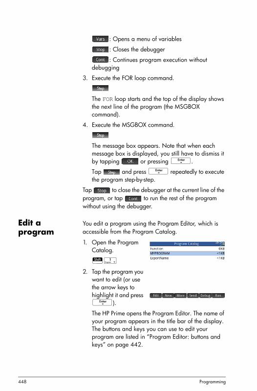
448 Programming
: Opens a menu of variables
: Closes the debugger
: Continues program execution without debugging
3. Execute the FOR loop command.
The FOR loop starts and the top of the display shows the next line of the program (the MSGBOX command).
4. Execute the MSGBOX command.
The message box appears. Note that when each message box is displayed, you still have to dismiss it by tapping or pressing E.
Tap and press E repeatedly to execute the program step-by-step.
Tap to close the debugger at the current line of the program, or tap to run the rest of the program without using the debugger.
Edit a program
You edit a program using the Program Editor, which is accessible from the Program Catalog.
1. Open the Program Catalog.
Sx
2. Tap the program you want to edit (or use the arrow keys to highlight it and press E).
The HP Prime opens the Program Editor. The name of your program appears in the title bar of the display. The buttons and keys you can use to edit your program are listed in “Program Editor: buttons and keys” on page 442.

Programming 449
Copy a program or part of a program
You can use the global Copy and Paste commands to copy part or all of a program. The following steps illustrate the process:
1. Open the Program Catalog.
Sx
2. Tap the program that has the code you want to copy.
3. Press SV (Copy).
The menu buttons change to give you options for copying:
: Marks where the copying or cutting is to begin.
: Marks where the copying or cutting is to end.
: Select the entire program.
: Cut the selection.
: Copy the selection.4. Select what you want to copy or cut (using the options
listed immediately above).
5. Tap or .
6. Return to the Program Catalog and open the target program.
7. Move the cursor to where you want to insert the copied or cut code.
8. Press SZ (Paste). The clipboard opens. What you most recently copied or cut will be first in the list and highlighted already, so just tap . The code will be pasted into the program, beginning at the cursor location.
Delete a program
To delete a program:
1. Open the Program Catalog.
Sx
2. Highlight a program to delete and press C.
3. At the prompt, tap to delete the program or to cancel.

450 Programming
Delete all programs
To delete all programs at once:
1. Open the Program Catalog.
Sx
2. Press SJ (Clear).
3. At the prompt, tap to delete all programs or to cancel.
Delete the contents of a program
You can clear the contents of a program without deleting the program. The program then just has a name and nothing else.
1. Open the Program Catalog.
Sx
2. Tap the program to open it.
3. Press SJ (Clear).
4. At the prompt, tap to delete the contents or to cancel.
The text of the program is deleted, but the program name remains.
To share a program
You can send programs between calculators just as you can send apps, notes, matrices, and lists. See “Sharing data” on page 40.
The HP Prime programming language
Variables and visibility
Variables in an HP Prime program can be used to store numbers, lists, matrices, graphics objects, and strings. The name of a variable must be a sequence of alphanumeric characters (letters and numbers), starting with a letter. Names are case-sensitive, so the variables named MaxTemp and maxTemp are different.
The HP Prime has built-in variables of various types, visible globally (that is, visible wherever you are in the calculator). For example, the built-in variables A to Z can be used to store real numbers, Z0 to Z9 can be used to store complex numbers, M0 to M9 can be used to store Matrices and vectors, and so on. These names are

Programming 451
reserved. You cannot use them for other data. For example, you cannot name a program M1, or store a real number in a variable named Z8. In addition to these reserved variables, each HP app has its own reserved variables. Some examples are Root, Xmin, and Numstart. Again, these names cannot be used to name a program. (A full list of system and app variables is given in chapter 21, “Variables”, beginning on page 373.)
In a program you can declare variables for use only within a particular function. This is done using a LOCAL declaration. The use of LOCAL variables enables you to declare and use variables that will not affect the rest of the calculator. LOCAL variables are not bound to a particular type, that is, you can store floating-point numbers, integers, lists, matrices, and symbolic expressions in a variable with any local name. Although the system will allow you to store different types in the same local variable, this is poor programming practice and should be avoided.
Variables declared in a program should have descriptive names. For example, a variable used to store the radius of a circle is better named RADIUS than VGFTRFG. You are more likely to remember what the variable is used for if its name matches its purpose.
If a variable is needed after the program executes, it can be exported from the program using the EXPORT command. To do this, the first command in the program (that is, on a line above the program name) would be EXPORT RADIUS. Then, if a value is assigned to RADIUS, the name appears on the variables menu (a) and is visible globally. This feature allows for extensive and powerful interactivity among different environments in the HP Prime. Note that if another program exports a variable with the same name, the most recently exported version will be active.
The program below prompts the user for the value of RADIUS, and exports the variable for use outside the program.
EXPORT RADIUS;
EXPORT GETRADIUS()
BEGIN

452 Programming
INPUT(RADIUS);
END;
Note that EXPORT command for the variable RADIUS appears before the heading of the function where RADIUS is assigned. After you execute this program, a new variable named RADIUS appears on the USER GETRADIUS section of the Variables menu.
Qualifying the name of a variable
The HP Prime has many system variables with names that are apparently the same. For example, the Function app has a variable named Xmin, but so too does the Polar app, the Parametric app, the Sequence app, and the Solve app. In a program, and in the Home view, you can refer to a particular version of these variables by qualifying its name. This is done by entering the name of the app (or program) that the variable belongs to, followed by a dot (.), and then the actual variable name. For example, the qualified variable Function.Xmin refers to the value of Xmin within the Function app. Similarly, the qualified variable Parametric.Xmin refers to the value of Xmin in the Parametric app. Despite having the same name—Xmin—the variables could have different values. You do likewise to declare a local variable in a program: specify the name of the program, followed by the dot, and then variable name.
Functions, their arguments, and parameters
You can define your own functions in a program, and data can be passed to a function using parameters. Functions can return a value (using the RETURN statement) or not. When a program is executed from Home view, the program will return the value returned by the last statement that was executed.
Furthermore, functions can be defined in a program and exported for use by other programs, in much the same way that variables can be defined and used elsewhere.

Programming 453
In this section, we will create a small set of programs, each illustrating some aspect of programming in the HP Prime. Each program will be used as a building block for a custom app described in the next section, App Programs.
Program ROLLDIE We’ll first create a program called ROLLDIE. It simulates the rolling of a single die, returning a random integer between 1 and whatever number is passed into the function.
In the Program Catalog create a new program named ROLLDIE. (For help, see page 441.) Then enter the code in the Program Editor.
EXPORT ROLLDIE(N)
BEGIN
RETURN 1+FLOOR(RANDOM(N));
END;
The first line is the heading of the function. Execution of the RETURN statement causes a random integer from 1 to N to be calculated and returned as the result of the function. Note that the RETURN command causes the execution of the function to terminate. Thus any statements between the RETURN statement and END are ignored.
In Home view (in fact, anywhere in the calculator where a number can be used), you can enter ROLLDIE(6) and a random integer between 1 and 6 inclusive will be returned.
Program ROLLMANY
Another program could use the ROLLDIE function, and generate n rolls of a die with any number of sides. In the following program, the ROLLDIE function is used to generate n rolls of two dice, each with the number of sides given by the local variable sides. The results are stored in list L2, so that L2(1) shows the number of times the dies came up with a combined total of 1, L2(2) shows the number of times the dies came up with a combined total of 2, etc. L2(1) should be 0 (since the sum of the numbers on 2 dice must be at least 2).
EXPORT ROLLMANY(n,sides)
BEGIN
LOCAL k,roll;

454 Programming
// initialize list of frequencies
MAKELIST(0,X,1,2*sides,1)L2;
FOR k FROM 1 TO n DO
ROLLDIE(sides)+ROLLDIE(sides)roll;
L2(roll)+1L2(roll);
END;
END;
By omitting the EXPORT command when a function is declared, its visibility can be restricted to the program within which it is defined. For example, you could define the ROLLDIE function inside the ROLLMANY program like this:
ROLLDIE();
EXPORT ROLLMANY(n,sides)
BEGIN
LOCAL k,roll;
// initialize list of frequencies
MAKELIST(0,X,1,2*sides,1)L2;
FOR k FROM 1 TO n DO
ROLLDIE(sides)+ROLLDIE(sides)roll;
L2(roll)+1L2(roll); END;
END;
ROLLDIE(n)
BEGIN
RETURN 1+FLOOR(RANDOM(N));
END;
In this scenario, assume there is no ROLLDIE function exported from another program. Instead, ROLLDIE is visible only to ROLLMANY. The ROLLDIE function must be declared before it is called. The first line of the program above contains the declaration of the ROLLDIE function. The definition of the ROLLDIE function is located at the end of the program.
Finally, the list of results could be returned as the result of calling ROLLMANY instead of being stored directly in the global list variable, L2. This way, if the user wanted to store the results elsewhere, it could be done easily.
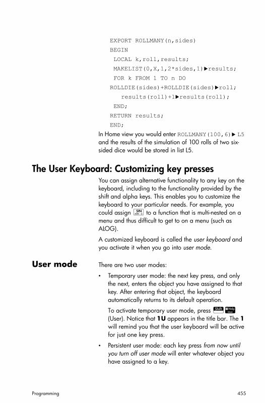
Programming 455
EXPORT ROLLMANY(n,sides)
BEGIN
LOCAL k,roll,results;
MAKELIST(0,X,1,2*sides,1)results;
FOR k FROM 1 TO n DO
ROLLDIE(sides)+ROLLDIE(sides)roll;
results(roll)+1results(roll); END;
RETURN results;
END;
In Home view you would enter ROLLMANY(100,6) L5 and the results of the simulation of 100 rolls of two six-sided dice would be stored in list L5.
The User Keyboard: Customizing key pressesYou can assign alternative functionality to any key on the keyboard, including to the functionality provided by the shift and alpha keys. This enables you to customize the keyboard to your particular needs. For example, you could assign e to a function that is multi-nested on a menu and thus difficult to get to on a menu (such as ALOG).
A customized keyboard is called the user keyboard and you activate it when you go into user mode.
User mode There are two user modes:
• Temporary user mode: the next key press, and only the next, enters the object you have assigned to that key. After entering that object, the keyboard automatically returns to its default operation.
To activate temporary user mode, press SW (User). Notice that 1U appears in the title bar. The 1 will remind you that the user keyboard will be active for just one key press.
• Persistent user mode: each key press from now until you turn off user mode will enter whatever object you have assigned to a key.

456 Programming
To activate persistent user mode, press SWSW. Notice that U appears in the title bar. The user keyboard will now remain active until you press SW again.
If you are in user mode and press a key that hasn’t been re-assigned, the key’s standard operation is performed.
Re-assigning keys
Suppose you want to assign a commonly used function—such as ALOG—to its own key on the keyboard. Simply create a new program that mimics the syntax in the image at the right.
The first line of the program specifies the key to be reassigned using its internal name. (The names of all the keys are given in “Key names” on page 456. They are case-sensitive.)
On line 3, enter the text you want produced when the key being re-assigned is pressed. This text must be enclosed in quote marks.
The next time you want to insert ALOG at the position of your cursor, you just press SWe.
You can enter any string you like in the RETURN line of your program. For example, if you enter “M4”, matrix M4 will be returned when you press the re-assigned key. You can even get the program to return user-defined functions as well as system functions, and user-defined variables as well as system variables.
You can also re-assign a shifted key combination. So, for example, ASn could be re-assigned to produce SLOPE(F1(X),3) rather than the lowercase t. Then if ASn is entered in Home view and E pressed, the gradient at X = 3 of whatever function is currently defined as F1(X) in the Function app would be returned.
Key names The first line of a program that re-assigns a key must specify the key to be reassigned using its internal name.

Programming 457
The table below gives the internal name for each key. Note that key names are case-sensitive.
Internal name of keys and key states
Key Name S+ key
A+ key
AS+ key
N K_0 KS_0 KA_0 KSA_0
x K_1 KS_1 KA_1 KSA_1
y K_2 KS_2 KA_2 KSA_2
z K_3 KS_3 KA_2 KSA_2
t K_4 KS_4 KA_4 KSA_4
u K_5 KS_5 KA_5 KSA_5
v K_6 KS_6 KA_6 KSA_6
p K_7 KS_7 KA_7 KSA_7
q K_8 KS_8 KA_8 KSA_8
r K_9 KS_9 KA_9 KSA_9
c K_Abc KS_Abc KA_Abc KSA_Abc
A K_Alpha KS_Alpha KA_Alpha KSA_Alpha
I K_Apps KS_Apps KA_Apps KSA_Apps
C K_Bksp KS_Bksp KA_Bksp KSA_Bksp
o K_Comma KS_Comma KA_Comma KSA_Comma
f K_Cos KS_Cos KA_Cos KSA_Cos
n K_Div KS_Div KA_Div KSA_Div
. K_Dot KS_Dot KA_Dot KSA_Dot
\ K_Down KS_Down KA_Down KSA_Down
E K_Enter KS_Enter KA_Enter KSA_Enter
H K_Home KS_Home KA_Home KSA_Home
,< K_Left KS_Left KA_Left KSA_Left
,> K_Right KS_Right KA_Right KSA_Right

458 Programming
h K_Ln KS_Ln KA_Ln KSA_Ln
i K_Log KS_Log KA_Log KSA_Log
w K_Minus KS_Minus KA_Minus KSA_Minus
Q K_Neg KS_Neg KA_Neg KSA_Neg
M K_Num KS_Num KA_Num KSA_Num
O K_On KS_On KA_On KSA_On
P K_Plot KS_Plot KA_Plot KSA_Plot
+ K_Plus KS_Plus KA_Plus KSA_Plus
k K_Power KS_Power KA_Power KSA_Power
e K_Sin KS_Sin KA_Sin KSA_Sin
j K_Sq KS_Sq KA_Sq KSA_Sq
Y K_Symb KS_Symb KA_Symb KSA_Symb
g K_Tan KS_Tan KA_Tan KSA_Tan
= K_Up KS_Up KA_Up KSA_Up
a K_Vars KS_Vars KA_Vars KSA_Vars
V K_View KS_View KA_View KSA_View
d K_Xttn KS_Xttn KA_Xttn KSA_Xttn
W
Z
J
K
D
F
R
B
Internal name of keys and key states
Key Name S+ key
A+ key
AS+ key

Programming 459
App programsAn app is a unified collection of views, programs, notes, and associated data. Creating an app program allows you to redefine the app’s views and how a user will interact with those views. This is done with (a) dedicated program functions with special names and (b) by redefining the views in the Views menu.
Using dedicated program functions
These programs are run when the keys shown in the table below are pressed. These program functions are designed to be used in the context of an app.
s
S
X
Internal name of keys and key states
Key Name S+ key
A+ key
AS+ key
Program Name Equivalent Keystrokes
Symb Symbolic view Y
SymbSetup Symbolic Setup SY
Plot Plot view P
PlotSetup Plot Setup SP
Num Numeric view M
NumSetup Numeric Setup SM
Info Info view SI
START Starts an app
RESET Resets or initializes an app

460 Programming
Redefining the Views menu
The Views menu allows any app to define views in addition to the standard seven views shown in the table above. By default, each HP app has its own set of additional views contained in this menu. The VIEWS command allows you to redefine these views to run programs you have created for an app. The syntax for the VIEWS command is:
VIEWS "text"
By adding VIEWS "text" before the declaration of a function, you will override the list of views for the app. For example, if your app program defines three views—"SetSides", "RollDice" and "PlotResults"—when you press V you will see SetSides, RollDice, and PlotResults instead of the app’s default view list.
Customizing an app
When an app is active, its associated program appears as the first item in the Program Catalog. It is within this program that you put functions to create a custom app. A useful procedure for customizing an app is illustrated below:
1. Decide on the HP app that you want to customize. The customized app inherits all the properties of the HP app.
2. Go to the Applications Library (A), highlight the HP app, tap and save the app with a unique name.
3. Customize the new app if you need to (for example, by configuring the axes or angle measure settings).
4. Develop the functions to work with your customized app. When you develop the functions, use the app naming conventions described above.
5. Put the VIEWS command in your program to modify the app's Views menu.
6. Decide if your app will create new global variables. If so, you should EXPORT them from a separate user program that is called from the Start() function in the app program. This way they will not have their values lost.
7. Test the app and debug the associated programs.

Programming 461
It is possible to link more than one app via programs. For example, a program associated with the Function app could execute a command to start the Statistics 1Var app, and a program associated with the Statistics 1Var app could return to the Function app (or launch any other app).
Example The following example illustrates the process of creating a custom app. The app is based on the built-in Statistics 1Var app. It simulates the rolling of a pair of dice, each with a number of sides specified by the user. The results are tabulated, and can be viewed either in a table or graphically.
1. In the Application Librray, select the Statistics 1Var app but don’t open it.
I Select Statistics 1Var.
2. Tap . 3. Enter a name for the new app (such as
DiceSimulation.)
4. Tap twice.
The new app appears in the Application Library.
5. Open the new app.
6. Open the Program Catalog.
Sx
7. Tap the program to open it.
Each customised app has one program associated with it. Initially, this program is empty. You customize the app by entering functions into that program.
At this point you decide how you want the user to interact with the app. In this example, we will want the user to be able to:

462 Programming
• start the app
• specify the number of sides (that is, faces) on each die
• specify number of times to roll the dice
• start the app again.
With that in mind, we will create the following views:
START, SETSIDES, and SETNUMROLLS.
The START option will initialize the app and display a note that gives the user instructions. The user will also interact with the app through the Numeric view and the Plot view. These views will be activated by pressing M and P, but the functions Num and Plot in our app program will actually launch those views after doing some configuration.
The program discussed earlier in this chapter to get the number of sides for a dice is expanded here, so that the possible sums of two such die are stored in dataset D1. Enter the following sub-routines into the program for the DiceSimulation app.
The program DiceSimulation
START()
BEGIN
DICESIMVARS();
{}D1;
{}D2;
SetSample(H1,D1);
SetFreq(H1,D2);
0H1Type;
END;
VIEWS "Roll Dice",ROLLMANY()
BEGIN
LOCAL k,roll;
MAKELIST(X+1,X,1,2*SIDES-1,1)D1;
MAKELIST(X+1,X,1,2*SIDES-1,1)D2;
FOR k FROM 1 TO ROLLS DO
roll:=ROLLDIE(SIDES)+ROLLDIE (SIDES);
D2(roll-1)+1D2(roll-1);
END;

Programming 463
-1Xmin;
MAX(D1)+1Xmax;
0Ymin;
MAX(D2)+1Ymax;
STARTVIEW(1,1);
END;
VIEWS "Set Sides",SETSIDES()
BEGIN
REPEAT
INPUT(SIDES,"Die Sides","N=","ENTER num sides",2);
FLOOR(SIDES)SIDES;
IF SIDES<2 THEN
MSGBOX("Must be >= 2");
END;
UNTIL SIDES >=2;
END;
VIEWS "Set Rolls",SETROLLS()
BEGIN
REPEAT
INPUT(ROLLS,"Num of rolls","N=","Enter numrolls",25);
FLOOR(ROLLS)ROLLS;
IF ROLLS<1 THEN
MSGBOX(" u must enter a num >=1");
END;
UNTIL ROLLS>=1;
END;
PLOT()
BEGIN
-1Xmin;
MAX(D1)+1Xmax;
0Ymin;
MAX(D2)+1Ymax;
STARTVIEW(1,1);
END;

464 Programming
The ROLLMANY() routine is an adaptation of the program presented earlier in this chapter. Since you cannot pass parameters to a program called through a selection from a custom Views menu, the exported variables SIDES and ROLLS are used in place of the parameters that were used in the previous versions.
The program above calls two other user programs: ROLLDIE() and DICESIMVARS(). ROLLDIE() appears earlier in this chapter. Here is DICESIMVARS. Create a program with that name and enter the following code.
The program DICESIMVARS
EXPORT ROLLS,SIDES;
EXPORT DICESIMVARS()
BEGIN
10 ROLLS;
6 SIDES;
END;
Press V to see the custom app menu. Here you can set the number of sides of the dice, the number of rolls, and execute a simulation.
After running a simulation, press P to see a histogram of your simulation results.
Program commandsThis section describes each program command. The commands under the menu are described first. The commands under the menu are described in “Commands under the Cmds menu” on page 470.
Doesn’t work in build 3105

Programming 465
Commands under the Tmplt menu
BlockThe block commands determine the beginning and end of a sub-routine or function. There is also a Return command to recall results from sub-routines or functions.
BEGIN END Syntax: BEGIN stmt1;stm2;…stmtN; END;
Defines a command or set of commands to be executed together. In the simple program:
EXPORT SQM1(X)
BEGIN
RETURN X^2-1;
END;
the block is the single RETURN command.
If you entered SQM1(8) in Home view, the result returned would be 63.
RETURN Syntax: RETURN expression;
Returns the current value of expression.
KILL Syntax: KILL;
Stops the step-by-step execution of the current program (with debug).
BranchIn what follows, the plural word commands refers to both a single command or a set of commands.
IF THEN Syntax: IF test THEN commands END;
Evaluate test. If test is true (not 0), execute commands. Otherwise, nothing happens.
IF THEN ELSE Syntax: IF test THEN commands1 ELSE commands 2 END;
Evaluate test. If test is true (non 0), execute commands 1, otherwise, execute commands 2
CASE Syntax:
CASE

466 Programming
IF test1 THEN commands1 END
IF test2 THEN commands2 END
…
[DEFAULT commands]
END;Evaluates test1. If true, execute commands1 and end the CASE. Otherwise, evaluate test2. If true, execute commands2. Continue evaluating tests until a true is found. If no true test is found, execute default commands, if provided.
Example:
CASE
IF THEN RETURN "negative"; END
IF THEN RETURN "small"; END
DEFAULT RETURN "large";
END;
IFERR IFERR commands1 THEN commands2 [ELSE commands3] END;
Executes sequence of commands1. If an error occurs during execution of commands1, executes sequence of commands2.
IFERR ELSE IFERR commands1 THEN commands2 ELSE commands3 END;
Executes sequence of commands1. If an error occurs during execution of commands1, executes sequence of commands2. Otherwise, execute sequence of commands3.
LoopFOR Syntax: FOR var FROM start TO finish DO commands
Sets variable var to start, and for as long as this variable is less than or equal to finish, executes the sequence of commands, and then adds 1 (increment) to var. If DOWNTO is used the start value of the variable is decreased until the finish value is reached.
x 0
x 1

Programming 467
Example 1: This program determines which integer from 2 to N has the greatest number of factors.
EXPORT MAXFACTORS(N)
BEGIN
LOCAL cur, max,k,result;
1 max;1 result;
FOR k FROM 2 TO N DO
SIZE(idivis(k)) cur;
IF cur > max THEN
cur max; k result; END;END;
MSGBOX("Max of "+ max +" factors for "+result);
In Home, enter MAXFACTORS(100).
This syntax is not working as at build 3015.
FOR STEP Syntax: FOR var FROM start TO finish [STEP increment] DO commands
Sets variable var to start, and for as long as this variable is less than or equal to finish, executes the sequence of commands, and then adds 1 (increment) to var.
Example 2: This program draws an interesting pattern on the screen.
EXPORT DRAWPATTERN()
BEGIN
LOCAL xincr,yincr,color;
STARTAPP("Function");
RECT();
xincr := (Xmax - Xmin)/254;
yincr := (Ymax - Ymin)/110;
FOR X FROM Xmin TO Xmax STEP xincr DO

468 Programming
FOR Y FROM Ymin TO Ymax STEP yincr DO color := FLOOR(X^2+Y^2) MOD 4; PIXON(X,Y,color);END;
END;
FREEZE;
END;
FOR DOWN Syntax: FOR var FROM start DOWNTO finish DO commands
Sets variable var to start, and for as long as this variable is less than or equal to finish, executes the sequence of commands, and then adds 1 (increment) to var. If DOWNTO is used the start value of the variable is decreased until the finish value is reached.
FOR DOWN STEP Syntax: FOR var FROM start DOWNTO finish [STEP increment] DO commands
Sets variable var to start, and for as long as this variable is less than or equal to finish, executes the sequence of commands, and then adds 1 (increment) to var. If DOWNTO is used the start value of the variable is decreased until the finish value is reached.
WHILE Syntax: WHILE test DO commands END;
Evaluate test. If result is true (not 0), executes the commands, and repeat.
Example: A perfect number is one that is equal to the sum of all its proper divisors. For example, 6 is a perfect number because 6 = 1+2+3. The example below returns true when its argument is a perfect number.
EXPORT ISPERFECT(n)
BEGIN
LOCAL d, sum;
2 d;
1 sum;
WHILE sum < = n AND d < n DO
IF irem(n,d)==0 THEN

Programming 469
sum+d sum; END; d+1 d; END;
RETURN sum==n;
END;
The following program displays all the perfect numbers up to 1000:
EXPORT PERFECTNUMS()
BEGIN
LOCAL k;
FOR k FROM 2 TO 1000 DO
IF ISPERFECT(k) THEN
MSGBOX(k+" is perfect, press OK"); END;
END;
END;
REPEAT Syntax: REPEAT commands UNTIL test;
Repeats the sequence of commands until test is true (not 0).
The example below prompts for a positive value for SIDES, modifying an earlier program in this chapter:
EXPORT SIDES;
EXPORT GETSIDES()
BEGIN
REPEAT
INPUT(SIDES,"Die Sides","N = ","Enter num sides",2);
UNTIL SIDES>0;
END;
BREAK Syntax: BREAK(n)
Exits from loops by breaking out of n loop levels. Execution picks up with the first statement after the loop. With no argument exit from a single loop.
CONTINUE Syntax: CONTINUE

470 Programming
Transfer execution to the start of the next iteration of a loop.
VariableThese commands enable you to control the visibility of a user-defined variable.
LOCAL Local.
Syntax: LOCAL var1,var2,…varn;
Makes the variables var1, var2, etc. local to the program in which they are found.
EXPORT Exports the variable so that it is globally available.
FunctionThese commands enable you to control the visibility of a user-defined function.
EXPORT Export.
Syntax: EXPORT(FunctionName)
Exports the function FunctionName so that it is globally available and appears on the User menu (D ).
VIEW Sets text that the user can see by pressing V.
KEY A prefix to a key name when creating a user keyboard. See “The User Keyboard: Customizing key presses” on page 455.
Commands under the Cmds menu
StringsA string is a sequence of characters enclosed in double quotes (""). To put a double quote in a string, use two consecutive double quotes. The \ character starts an escape sequence, and the character(s) immediately following are interpreted specially. \n inserts a new line and two backslashes insert a single backslash. To put a new line into the string, press E to wrap the text at that point.
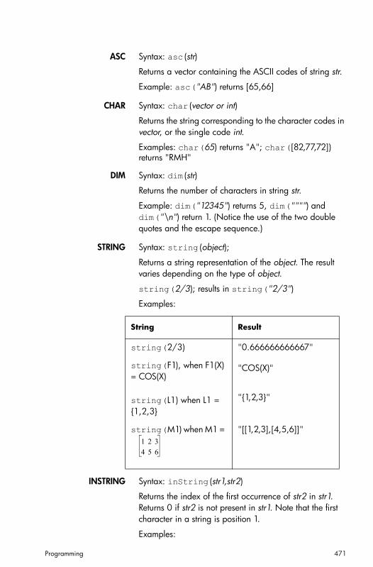
Programming 471
ASC Syntax: asc (str)
Returns a vector containing the ASCII codes of string str.
Example: asc("AB") returns [65,66]
CHAR Syntax: char (vector or int)
Returns the string corresponding to the character codes in vector, or the single code int.
Examples: char(65) returns "A"; char([82,77,72]) returns "RMH"
DIM Syntax: dim (str)
Returns the number of characters in string str.
Example: dim("12345") returns 5, dim("""") and dim("\n") return 1. (Notice the use of the two double quotes and the escape sequence.)
STRING Syntax: string (object);
Returns a string representation of the object. The result varies depending on the type of object.
string(2/3); results in string("2/3")
Examples:
INSTRING Syntax: inString (str1,str2)
Returns the index of the first occurrence of str2 in str1. Returns 0 if str2 is not present in str1. Note that the first character in a string is position 1.
Examples:
String Result
string(2/3) "0.666666666667"
string(F1), when F1(X) = COS(X)
"COS(X)"
string(L1) when L1 = {1,2,3}
"{1,2,3}"
string(M1) when M1 = "[[1,2,3],[4,5,6]]"1 2 3
4 5 6

472 Programming
inString("vanilla","van") returns 1.
inString ("banana","na") returns 3
inString("ab","abc") returns 0
LEFT Syntax: left (str,n)
Return the first n characters of string str. If or , returns str. If n == 0 returns the empty string.
Example: left("MOMOGUMBO",3) returns "MOM"
RIGHT Syntax: right(str,n)
Returns the last n characters of string str. If n <= 0, returns empty string. If n > –dim(str), returns str
Example: right("MOMOGUMBO",5) returns "GUMBO"
MID Syntax: mid(str,pos, [n])
Extracts n characters from string str starting at index pos. n is optional, if not specified, extracts all the remainder of the string.
Example: mid("MOMOGUMBO",3,5) returns "MOGUM", mid("PUDGE",4) returns "GE"
ROTATE Syntax: rotate(str,n)
Permutation of characters in string str. If 0 <=n < dim(str), shifts n places to left. If –dim(str) < n <= –1, shifts n spaces to right. If n > dim(str) or n < -dim(str), returns str.
Examples:
rotate("12345",2) returns "34512" rotate("12345",-1) returns "51234" rotate("12345",6) returns "12345"
STRINGFROMID Syntax: STRINGFROMID(integer)
Returns, in the current language, the built-in string associated in the internal string table with the specified integer.
Examples:
STRINGFROMID(56) returns “Complex”
STRINGFROMID(202) returns “Home Vars”
REPLACE Syntax: REPLACE(object1, start, object2)
n dim str n 0

Programming 473
Replaces part of object1 with object2 beginning at start. The objects can be matrices, vectors, or stings.
Example:
REPLACE("12345",3,”99”) returns "12995"
DrawingThere are 10 built-in graphics variables in the HP Prime, called G0–G9. G0 is always the current screen graphic.
G1 to G9 can be used to store temporary graphic objects (called GROBs for short) when programming applications that use graphics. They are temporary and thus cleared when the calculator turns off.
Twenty-six functions can be used to modify graphics variables. Thirteen of them work with Cartesian coordinates using the Cartesian plane defined in the current app by the variables Xmin, Xmax, Ymin, and Ymax.
The remaining thirteen work with pixel coordinates where the pixel 0,0 is the top left pixel of the GROB, and 255,126 is the bottom right. Functions in this second set have a _P suffix to the function name.
C→PX Converts from Cartesian coordinates to screen coordinates.
DRAWMENU Syntax: DRAWMENU({text1, text2, …})
Draws a menu showing the text items listed.
FREEZE Syntax: FREEZE
Pauses program execution until a key is pressed. This prevents the screen from being redrawn after the end of the program execution, leaving the modified display on the screen for the user to see.
PX→C Converts from screen coordinates to Cartesian coordinates.
Pixels and Cartesian
ARC_P
ARC Syntax; ARC(G, x, y, r [ , a1, a2, c])

474 Programming
ARC_P(G, x, y, r [ , a1, a2, c])
Draws an arc or circle on G, centered on point x,y, with radius r and color c starting at angle a1 and ending on angle a2.
G can be any of the graphics variables and is optional. The default is G0
r is given in pixels.
c is optional and if not specified black is used.
a1 and a2 follow the current angle mode and are optional. The default is a full circle.
BLIT_P
BLIT Syntax: BLIT([trgtGRB, dx1, dy1, dx2, dy2],
srcGRB [ ,sx1, sy1, sx2, sy2, c])
BLIT_P ([trgtGRB, dx1, dy1, dx2, dy2],
srcGRB [ ,sx1, sy1, sx2, sy2, c])
Copies the region of srcGRB between point sx1, sy1 and sx2, sy2 into the region of trgtGRB between points dx1, dy1 and dx2, dy2. Do not copy pixels from srcGRB that are color c.
trgtGRB can be any of the graphics variables. trgtGRB can be any of the graphics variables and is optional. The default is G0.
srcGRB can be any of the graphics variables.
dx2, dy2 are optional and if not specified will be calculated so that the destination area is the same size as the source area.
sx2, sy2 are optional and if not specified will be the bottom right of the srcGRB.
sx1, sy1 are optional and if not specified will be the top left of srcGRB.
dx1, dy1 are optional and if not specified will be the top left of trgtGRB.
c can be 0 to 3 (0=black, 1= dark gray, 2= light gray, 3= white). c is optional. If not specified all pixels from G2 will be copied.
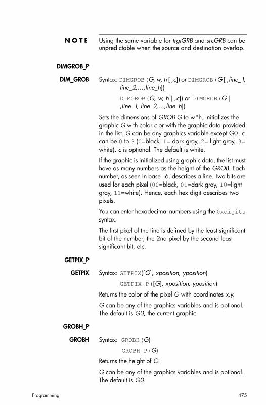
Programming 475
N O T E Using the same variable for trgtGRB and srcGRB can be unpredictable when the source and destination overlap.
DIMGROB_P
DIM_GROB Syntax: DIMGROB(G, w, h [ ,c]) or DIMGROB(G [ ,line_1, line_2,…,line_h])
DIMGROB(G, w, h [ ,c]) or DIMGROB(G [ ,line_1, line_2,…,line_h])
Sets the dimensions of GROB G to w*h. Initializes the graphic G with color c or with the graphic data provided in the list. G can be any graphics variable except G0. c can be 0 to 3 (0=black, 1= dark gray, 2= light gray, 3= white). c is optional. The default is white.
If the graphic is initialized using graphic data, the list must have as many numbers as the height of the GROB. Each number, as seen in base 16, describes a line. Two bits are used for each pixel (00=black, 01=dark gray, 10=light gray, 11=white). Hence, each hex digit describes two pixels.
You can enter hexadecimal numbers using the 0xdigits syntax.
The first pixel of the line is defined by the least significant bit of the number; the 2nd pixel by the second least significant bit, etc.
GETPIX_P
GETPIX Syntax: GETPIX([G], xposition, yposition)
GETPIX_P([G], xposition, yposition)
Returns the color of the pixel G with coordinates x,y.
G can be any of the graphics variables and is optional. The default is G0, the current graphic.
GROBH_P
GROBH Syntax: GROBH(G)
GROBH_P(G)
Returns the height of G.
G can be any of the graphics variables and is optional. The default is G0.

476 Programming
GROBW_P
GROBW Syntax: GROBW(G)
GROBW_P(G)
Returns the width of G.
G can be any of the graphics variables and is optional. The default is G0.
INVERT_P
INVERT Syntax: INVERT([G, x1, y1, x2, y2])
INVERT_P([G, x1, y1, x2, y2])
Inverts a rectangle on G between points x1,y1 and x2,y2. This means that every black pixel becomes white and vice-versa. In the same way Light gray and dark gray are inverted. G can be any of the graphics variables and is optional. The default is G0.
x2, y2 are optional and if not specified will be the bottom right of the graphic.
x1, y1 are optional and if not specified will be the top left of the graphic. If only one x,y pair is specified, it refers to the top left.
LINE_P
LINE Syntax: LINE(G, x1, y1, x2, y2, c)
LINE_P(G, x1, y1, x2, y2, c)
Draws a line of color c on G between points x1,y1 and x2,y2.
G can be any of the graphics variables and is optional. The default is G0.
c can be 0 to 3 (0=black, 1= dark gray, 2= light gray, 3= white). c is optional. The default is black.
PIXOFF_P
PIXOFF Syntax: PIXOFF([G], xposition, yposition)
PIXOFF_P([G], xposition, yposition)
Sets the color of the pixel G with coordinates x,y to white. G can be any of the graphics variables and is optional. The default is G0, the current graphic

Programming 477
PIXON_P
PIXON Syntax: PIXON([G], xposition, yposition [ ,color])
PIXON_P([G], xposition, yposition [ ,color])
Sets the color of the pixel G with coordinates x,y to color. G can be any of the graphics variables and is optional. The default is G0, the current graphic. Color can be 0 to 3 (0=black, 1= dark gray, 2= light gray, 3= white) and is optional. The default is 0.
RECT_P
RECT Syntax: RECT([G, x1, y1, x2, y2, edgecolor, fillcolor])
RECT_P([G, x1, y1, x2, y2, edgecolor, fillcolor])
Draws a rectangle on G between points x1,y1 and x2,y2 using edgecolor for the perimeter and fillcolor for the inside.
G can be any of the graphics variables and is optional. The default is G0, the current graphic.
x1, y1 are optional. The default values represent the top left of the graphic.
x2, y2 are optional. The default values represent the bottom right of the graphic.
edgecolor and fillcolor can be -1 to 3 (-1= transparent, 0=black, 1= dark gray, 2= light gray, 3= white).
edgecolor is optional. The default is white.
fillcolor is optional. The default is edgecolor.
To erase a GROB, execute RECT(G). To clear the screen execute RECT().
When optional arguments are provided in a command with multiple optional parameters (like RECT), the arguments provided correspond to the leftmost parameters first. For example, in the program below, the arguments 40 and 90 in the RECT_P command correspond to x1 and y1. The argument 0 corresponds to edgecolor, since there is only the one additional argument. If there had been two additional arguments, they would have referred to x2 and y2 rather than edgecolor and fillcolor. The program produces the figure below.
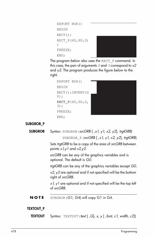
478 Programming
EXPORT BOX()
BEGIN
RECT();
RECT_P(40,90,0);
FREEZE;
END;
The program below also uses the RECT_P command. In this case, the pair of arguments 0 and 3 correspond to x2 and y2. The program produces the figure below to the right.
EXPORT BOX()
BEGIN
RECT();INVERT(G0);
RECT_P(40,90,0,3);
FREEZE;
END;
SUBGROB_P
SUBGROB Syntax: SUBGROB(srcGRB [ ,x1, y1, x2, y2], trgtGRB)
SUBGROB_P(srcGRB [ ,x1, y1, x2, y2], trgtGRB)
Sets trgtGRB to be a copy of the area of srcGRB between points x1,y1 and x2,y2.
srcGRB can be any of the graphics variables and is optional. The default is G0.
trgtGRB can be any of the graphics variables except G0.
x2, y2 are optional and if not specified will be the bottom right of srcGRB.
x1, y1 are optional and if not specified will be the top left of srcGRB.
N O T E SUBGROB(G1, G4) will copy G1 in G4.
TEXTOUT_P
TEXTOUT Syntax: TEXTOUT(text [ ,G], x, y [ ,font, c1, width, c2])

Programming 479
TEXTOUT_P(text [ ,G], x, y [ ,font, c1, width, c2])
Draws text using color c1 on graphic G at position x, y using font. Do not draw text more than width pixels wide and erase the background before drawing the text using color c2. G can be any of the graphics variables and is optional. The default is G0.
Font can be:
0: current font selected in mode screen, 1: small font 2: large font. Font is optional and if not specified is the current font selected in mode screen.
c1 can be 0 to 3 (0=black, 1= dark gray, 2= light gray, 3= white). c1 is optional. The default is black.
width is optional and if not specified, no clipping is performed.
c2 can be 0 to 3 (0=black, 1= dark gray, 2= light gray, 3= white). c2 is optional. If not specified the background is not erased.
Example:
This program displays the successive approximations for using the series for the arctangent(1).
EXPORT RUNPISERIES()
BEGIN
LOCAL sign;
2 K;4 A;
-1 sign;
RECT();
TEXTOUT_P("N=",0,0);
TEXTOUT_P("PI APPROX=",0,30);
REPEAT
A+sign*4/(2*K-1) A;
TEXTOUT_P(K ,35,0,2,0,100,3);TEXTOUT_P(A ,90,30,2,0,100,3);

480 Programming
sign*-1 sign;
K+1 K;
UNTIL 0;
END;
The program executes until the user presses O to terminate. The spaces after K (the number of the term) and A (the current approximation) in the TEXTOUT_P commands are there to overwrite the previously displayed value.
MatrixSome matrix commands take as their argument the matrix variable name on which the command is applied. Valid names are the global variables M0–M9 or a local variable that contains a matrix.
ADDCOL Syntax: ADDCOL
(name [ ,value1,...,valuen],column_number)
Inserts values into a new column inserted before column_number in the specified matrix. You enter the values as a vector. (These are not optional arguments.) The values must be separated by commas and the number of values must be the same as the number of rows in the matrix name.
ADDROW Syntax: ADDROW
(name [ ,value1,...,valuen],row_number)
Inserts values into a new row inserted before row_number in the specified matrix. You enter the values as a vector. (These are not optional arguments.) The values must be separated by commas and the number of values must be the same as the number of columns in the matrix name.
DELCOL Syntax: DELCOL(name ,column_number)
Deletes column column_number from matrix name.
DELROW Syntax: DELROW(name ,row_number)
Deletes row row_number from matrix name.

Programming 481
EDITMAT Syntax: EDITMAT(name)
Starts the Matrix Editor and displays the specified matrix. If used in programming, returns to the program when user presses . Even though this command returns the matrix that was edited, EDITMAT cannot be used as an argument in other matrix commands.
REDIM Syntax: REDIM(name, size)
Redimensions the specified matrix (name) or vector to size. For a matrix, size is a list of two integers (n1,n2). For a vector, size is a list containing one integer (n). Existing values in the matrix are preserved. Fill values will be 0.
REPLACE Syntax: REPLACE(name, start, object)
Replaces portion of a matrix or vector stored in name with an object starting at position start. Start for a matrix is a list containing two numbers; for a vector, it is a single number. REPLACE also works with lists, graphics, and strings. For example, REPLACE("123456", 2, "GRM") -> "1GRM56"
SCALE Syntax: SCALE (name, value, rownumber)
Multiplies the specified row_number of the specified matrix by value.
SCALEADD Syntax: SCALEADD (name, value, row1, row2)
Multiplies the specified row1 of the matrix (name) by value, then adds this result to the second specified row2 of the matrix (name).
SUB Syntax: SUB (name, start, end)
Extracts a sub-object—a portion of a list, matrix, or graphic—and stores it in name. Start and end are each specified using a list with two numbers for a matrix, a number for vector or lists, or an ordered pair, (X,Y), for graphics: SUB(M1{1,2},{2,2})
SAWAPCOL Syntax: SWAPCOL (name, column1, column2)
Swaps column1 and column2 of the specified matrix (name).
SWAPROW Syntax: SWAPROW(name, row1, row2)
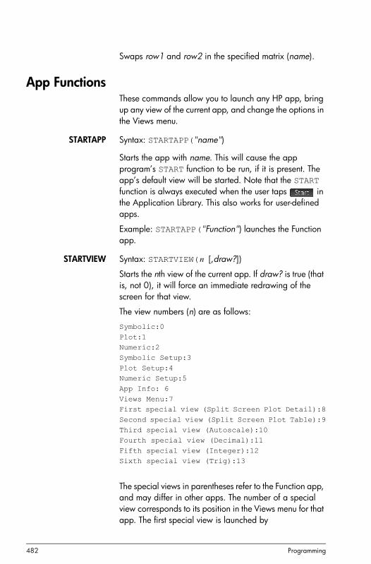
482 Programming
Swaps row1 and row2 in the specified matrix (name).
App FunctionsThese commands allow you to launch any HP app, bring up any view of the current app, and change the options in the Views menu.
STARTAPP Syntax: STARTAPP("name")
Starts the app with name. This will cause the app program’s START function to be run, if it is present. The app’s default view will be started. Note that the START function is always executed when the user taps in the Application Library. This also works for user-defined apps.
Example: STARTAPP("Function") launches the Function app.
STARTVIEW Syntax: STARTVIEW( [,draw?])
Starts the nth view of the current app. If draw? is true (that is, not 0), it will force an immediate redrawing of the screen for that view.
The view numbers (n) are as follows:
Symbolic:0Plot:1Numeric:2Symbolic Setup:3Plot Setup:4Numeric Setup:5App Info: 6Views Menu:7First special view (Split Screen Plot Detail):8Second special view (Split Screen Plot Table):9Third special view (Autoscale):10Fourth special view (Decimal):11Fifth special view (Integer):12Sixth special view (Trig):13
The special views in parentheses refer to the Function app, and may differ in other apps. The number of a special view corresponds to its position in the Views menu for that app. The first special view is launched by
n
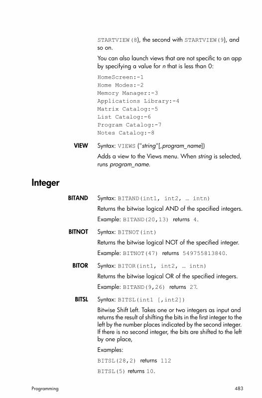
Programming 483
STARTVIEW(8), the second with STARTVIEW(9), and so on.
You can also launch views that are not specific to an app by specifying a value for n that is less than 0:
HomeScreen:-1Home Modes:-2 Memory Manager:-3 Applications Library:-4 Matrix Catalog:-5List Catalog:-6Program Catalog:-7Notes Catalog:-8
VIEW Syntax: VIEWS ("string"[,program_name])
Adds a view to the Views menu. When string is selected, runs program_name.
IntegerBITAND Syntax: BITAND(int1, int2, … intn)
Returns the bitwise logical AND of the specified integers.
Example: BITAND(20,13) returns 4.
BITNOT Syntax: BITNOT(int)
Returns the bitwise logical NOT of the specified integer.
Example: BITNOT(47) returns 549755813840.
BITOR Syntax: BITOR(int1, int2, … intn)
Returns the bitwise logical OR of the specified integers.
Example: BITAND(9,26) returns 27.
BITSL Syntax: BITSL(int1 [,int2])
Bitwise Shift Left. Takes one or two integers as input and returns the result of shifting the bits in the first integer to the left by the number places indicated by the second integer. If there is no second integer, the bits are shifted to the left by one place,
Examples:
BITSL(28,2) returns 112
BITSL(5) returns 10.

484 Programming
BITSR Syntax: BITRL(int1 [,int2])
Bitwise Shift Right. Takes one or two integers as input and returns the result of shifting the bits in the first integer to the right by the number places indicated by the second integer. If there is no second integer, the bits are shifted to the right by one place,
Examples:
BITSR(112,2) returns 28
BITSR(10) returns 5.
BITXOR Syntax: BITXOR(int1, int2, … intn)
Returns the bitwise logical exclusive OR of the specified integers.
Example: BITAND(9,26) returns 19.
B→R Syntax: B→R(#integerm)
Converts an integer in base m to a decimal integer (base 10). The base marker m can be b (for binary), o (for octal), or h (for hexadecimal).
Example: B→R(#1101b) returns 13
GETBASE Syntax: GETBASE(#integer[m])
Returns the base for the specified integer (in whatever is the current default base): 0 = default, 1 = binary, 2 = octal, 3 = hexadecimal.
Examples: GETBASE(#1101b) returns #1h (if the default base is hexadecimal) while GETBASE (#1101) returns #0h.
GETBITS Syntax: GETBITS(#integer)
Returns the number of bits used by integer, expressed in the default base.
Example: GETBITS(#22122) returns #20h (if the default base is hexadecimal)
R→B Syntax: R→B(integer)
Converts a decimal integer (base 10) to an integer in the default base.
Example: R→B(13) returns #1101b (if the default base is binary) or #Dh (if the default base is hexadecimal).
SETBITS Syntax: SETBITS(#integer[m] [,bits])

Programming 485
Sets the number of bits to represent integer. Valid values are in the range –64 to 65. If m or bits is omitted, the default value is used.
Example: SETBITS(#1111,b15) returns #1111b:15
SETBASE Syntax: SETBASE(#integer[m][c])
Displays integer expressed in base m in whatever base is indicated by c, where can be 1 (for binary), 2 (for octal), or 3 (for hexadecimal). Parameter m can be b (for binary), d (for decimal), o (for octal), or h (for hexadecimal). If m is omitted, the input is assumed to be in the default base. Likewise, if c is omitted, the output is displayed in the default base.
Examples: SETBASE (#34o,1) returns #11100b while GETBASE (#1101) returns #0h ((if the default base is hexadecimal).
I/OI/O commands are used for inputting data into a program, and for outputting data from a program. They allow users to interact with programs.
These commands start the Matrix and List editors.
CHOOSE Syntax: CHOOSE(var, "title", "item1", "item2",…,"itemn")
Displays a choose box with the title and containing the choose items. If the user selects an object, the variable whose name is provided will be updated to contain the number of the selected object (an integer, 1, 2, 3, …) or 0 if the user taps .
Returns true (not zero) if the user selects an object, otherwise return false (0).
Example:
CHOOSE
(N,"PickHero","Euler","Gauss","Newton");
IF N==1 THEN PRINT("You picked Euler"); ELSE IF N==2 THEN PRINT("You picked

486 Programming
Gauss");ELSE PRINT("You picked Newton");
END;
END;
After execution of CHOOSE, the value of n will be updated to contain 0, 1, 2, or 3. The IF THEN ELSE command causes the name of the selected person to be printed to the terminal.
EDITLIST Syntax: EDITLIST(listvar)
Starts the List Editor loading listvar and displays the specified list. If used in programming, returns to the program when user taps .
Example: EDITLIST(L1) edits list L1.
EDITMAT Syntax: EDITMAT(matrixvar)
Starts the Matrix Editor and displays the specified matrix. If used in programming, returns to the program when user taps .
Example: EDITMAT(M1) edits matrix M1.
GETKEY Syntax: GETKEY
Returns the ID of the first key in the keyboard buffer, or –1 if no key was pressed since the last call to GETKEY. Key IDs are integers from 0 to 50, numbered from top left (key 0) to bottom right (key 50) as shown in figure 26-1.

Programming 487
INPUT Syntax: INPUT(var [,"title", "label", "help", default]);
Opens a dialog box with the title text title, with one field named label, displaying help at the bottom and using the default value. Updates the variable var if the user taps
and returns 1. If the user taps , it does not update the variable, and returns 0.
Example:
EXPORT SIDES;
EXPORT GETSIDES()
BEGIN
INPUT(SIDES,"Die Sides","N = ","Enter num sides",2);
END;
ISKEYDOWN Syntax: ISKEYDOWN(key_id);
Keys 14–19
Keys 20–25
Keys 26–30
Keys 31–35
Keys 36–40
Keys 46–50
Keys 41–45
0 1
2
3 4
5 6 7 8
910
11
1213
Keys 0–13{
Figure 26-1: Numbers of the keys
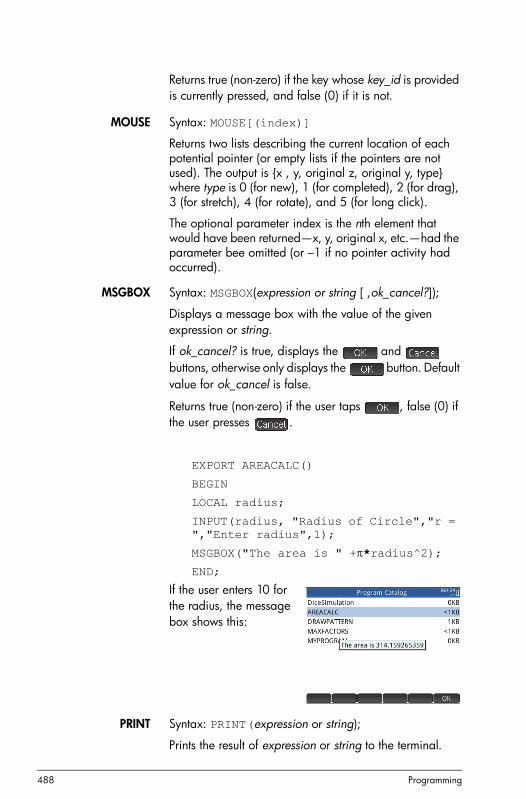
488 Programming
Returns true (non-zero) if the key whose key_id is provided is currently pressed, and false (0) if it is not.
MOUSE Syntax: MOUSE[(index)]
Returns two lists describing the current location of each potential pointer (or empty lists if the pointers are not used). The output is {x , y, original z, original y, type} where type is 0 (for new), 1 (for completed), 2 (for drag), 3 (for stretch), 4 (for rotate), and 5 (for long click).
The optional parameter index is the nth element that would have been returned—x, y, original x, etc.—had the parameter bee omitted (or –1 if no pointer activity had occurred).
MSGBOX Syntax: MSGBOX(expression or string [ ,ok_cancel?]);
Displays a message box with the value of the given expression or string.
If ok_cancel? is true, displays the and buttons, otherwise only displays the button. Default value for ok_cancel is false.
Returns true (non-zero) if the user taps , false (0) if the user presses .
EXPORT AREACALC()
BEGIN
LOCAL radius;
INPUT(radius, "Radius of Circle","r = ","Enter radius",1);
MSGBOX("The area is " +*radius^2);
END;
If the user enters 10 for the radius, the message box shows this:
PRINT Syntax: PRINT(expression or string);
Prints the result of expression or string to the terminal.
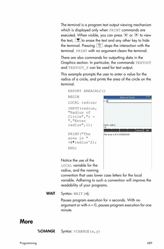
Programming 489
The terminal is a program text output viewing mechanism which is displayed only when PRINT commands are executed. When visible, you can press \ or = to view the text, Cto erase the text and any other key to hide the terminal. Pressing O stops the interaction with the terminal. PRINT with no argument clears the terminal.
There are also commands for outputting data in the Graphics section. In particular, the commands TEXTOUT and TEXTOUT_P can be used for text output.
This example prompts the user to enter a value for the radius of a circle, and prints the area of the circle on the terminal.
EXPORT AREACALC()
BEGIN
LOCAL radius;
INPUT(radius, "Radius of Circle","r = ","Enter radius",1);
PRINT("The area is " +*radius^2);
END;
Notice the use of the LOCAL variable for the radius, and the naming convention that uses lower case letters for the local variable. Adhering to such a convention will improve the readability of your programs.
WAIT Syntax: WAIT(n);
Pauses program execution for n seconds. With no argument or with n = 0, pauses program execution for one minute.
More%CHANGE Syntax: %CHANGE(x,y)
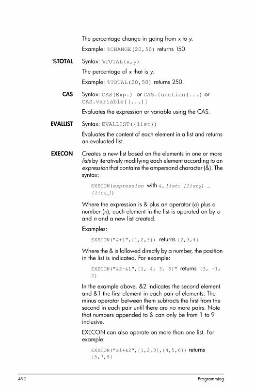
490 Programming
The percentage change in going from x to y.
Example: %CHANGE(20,50) returns 150.
%TOTAL Syntax: %TOTAL(x,y)
The percentage of x that is y.
Example: %TOTAL(20,50) returns 250.
CAS Syntax: CAS(Exp.) or CAS.function(...) or CAS.variable[(...)]
Evaluates the expression or variable using the CAS.
EVALLIST Syntax: EVALLIST({list})
Evaluates the content of each element in a list and returns an evaluated list.
EXECON Creates a new list based on the elements in one or more lists by iteratively modifying each element according to an expression that contains the ampersand character (&). The syntax:
EXECON(expression with &,list1 [list2] … [listn])
Where the expression is & plus an operator (o) plus a number (n), each element in the list is operated on by o and n and a new list created.
Examples:
EXECON("&+1",{1,2,3}) returns {2,3,4}
Where the & is followed directly by a number, the position in the list is indicated. For example:
EXECON("&2–&1",{1, 4, 3, 5}" returns {3, –1, 2}
In the example above, &2 indicates the second element and &1 the first element in each pair of elements. The minus operator between them subtracts the first from the second in each pair until there are no more pairs. Note that numbers appended to & can only be from 1 to 9 inclusive.
EXECON can also operate on more than one list. For example:
EXECON("&1+&2",{1,2,3},{4,5,6}) returns {5,7,9}

Programming 491
In the example above, &1 indicates an element in the first list and &2 indicates the corresponding element in the second list. The plus operator between them adds the two elements until there are no more pairs. Note that numbers appended to & can only be from 1 to 9 inclusive.
EXECON can also begin operating on a specified element in a specified list. For example:
EXECON("&23+&1",{1,5,16},{4,5,6,7}) returns {7,12}
In the example above, &23 indicates that operations are to begin on the second list and with the third element. To that element is added the first element in the first list. The process continues until there are no more pairs.
Again, the digits appended to & can only be from 1 to 9 inclusive.
→HMS Syntax: →HMS(value)
Converts a decimal value to hexagesimal format; that is, in units subdivided into groups of 60. This includes degrees, minutes, and seconds as well as hours, minutes, and seconds.
Example: →HMS(54.8763) returns 54°52′34.68″
HMS→ Syntax: HMS→(value)
Converts a value expressed hexagesimal format to decimal format.
Example: HMS→(54°52′34.68″) returns 54.8763
ITERATE Syntax: ITERATE(expr, var, ivalue, #times)
For #times, repeatedly evaluate expr in terms of var beginning with var = ivalue.
Example: ITERATE(X^2, X, 2, 3) returns 256
TICKS Syntax: TICKS
Returns the internal clock value in milliseconds.
TIME Syntax: TIME(program_name)
Returns the time in milliseconds required to execute the program program_name. The results are stored in the variable TIME. The variable TICKS is similar. It contains the number of milliseconds since boot up.

492 Programming
Variables and ProgramsThe HP Prime has four types of variables: Home variables, App variables, CAS variables, and User variables. You can retrieve these variables from the Variable menu (a).
Home variables are used for real numbers, complex numbers, graphics, lists, and matrices among other things. Home variables keep the same value in Home and in apps.
App variables are those whose values depend on the current app. The app variables are used in programming to represent the definitions and settings you make when working with apps interactively.
CAS variables are exactly the same as Home variables except that they are used only when doing CAS operations. They can, however, be called by commands in Home view. The names for CAS variables mirror those for Home variables except that they must be lowercase.
User variables are variables created by the user or exported from a user program. They provide one of several mechanisms to allow programs to communicate with the rest of the calculator, and with other programs. Once a variable has been exported from a program, it will appear among the User variables in the Variables menu, next to the program that exported it.
This chapter deals with App variables and User variables. For information on Home and CAS variables, see chapter 21, “Variables”, beginning on page 373.
App variables
Not all app variables are used in every app. S1Fit, for example, is only used in the Statistics 2Var app. However, most of the variables are used in common by the Function app, the Parametric app, the Polar app, the Sequence app, the Solve app, the Statistics 1Var app, the Statistics 2Var app, and others. If a variable is not available in all of these apps, or is available only in some other apps, then a list of the apps where the variable can be used appears under the variable name.
The following sections list the app variables by the view in which they are used. To see the variables listed by the
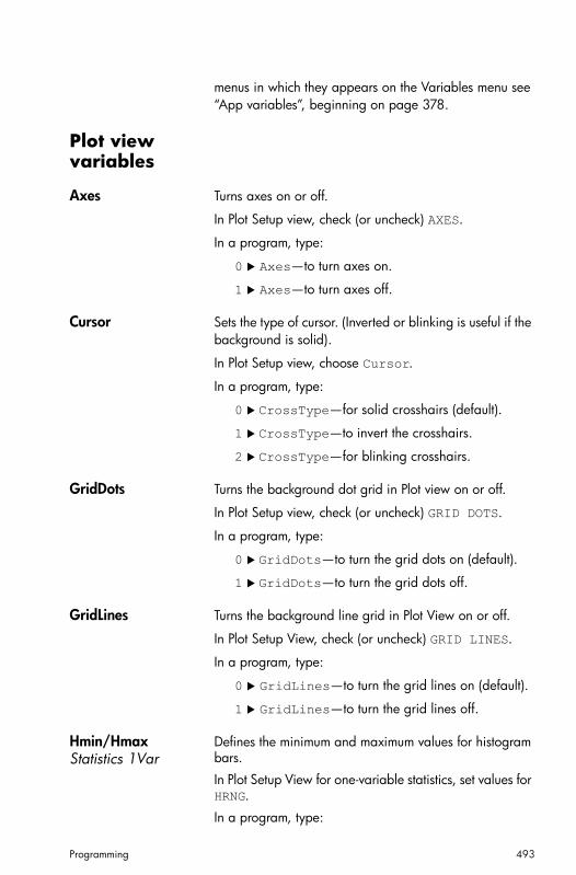
Programming 493
menus in which they appears on the Variables menu see “App variables”, beginning on page 378.
Plot view variables
Axes Turns axes on or off.
In Plot Setup view, check (or uncheck) AXES.
In a program, type:
0 Axes—to turn axes on.
1 Axes—to turn axes off.
Cursor Sets the type of cursor. (Inverted or blinking is useful if the background is solid).
In Plot Setup view, choose Cursor.
In a program, type:
0 CrossType—for solid crosshairs (default).
1 CrossType—to invert the crosshairs.
2 CrossType—for blinking crosshairs.
GridDots Turns the background dot grid in Plot view on or off.
In Plot Setup view, check (or uncheck) GRID DOTS.
In a program, type:
0 GridDots—to turn the grid dots on (default).
1 GridDots—to turn the grid dots off.
GridLines Turns the background line grid in Plot View on or off.
In Plot Setup View, check (or uncheck) GRID LINES.
In a program, type:
0 GridLines—to turn the grid lines on (default).
1 GridLines—to turn the grid lines off.
Hmin/HmaxStatistics 1Var
Defines the minimum and maximum values for histogram bars.
In Plot Setup View for one-variable statistics, set values for HRNG.
In a program, type:

494 Programming
Hmin
Hmax
where
HwidthStatistics 1Var
Sets the width of histogram bars.
In Plot Setup View for one-variable statistics, set a value for Hwidth.
In a program, type:n Hwidth
Labels Draws labels in Plot View showing X and Y ranges.
In Plot Setup View, check (or uncheck) Labels.
In a program, type:
1 Labels—to turn labels on (default)
0 Labels—to turn labels off.
Method Defines the graphing method: adaptive, fixed-step segments, or fixed-step dots. (See “Graphing methods” on page 89 for an explanation of the difference between these methods.)
In a program, type:
0 Method—select adaptive
1 Method—select fixed-step segments
2 Method—select fixed-step dots
Nmin/NmaxSequence
Defines the minimum and maximum values for the independent variable.
Appears as the NRNG fields in the Plot Setup view. In Plot Setup View, enter values for NRNG.
In a program, type:
Nmin
Nmax
where
Recenter Recenters at the cursor when zooming.
From Plot-Zoom-Set Factors, check (or uncheck) Recenter.
In a program, type:
n1
n2
n1 n2
n1
n2
n1 n2

Programming 495
0 Recenter— to turn recenter on (default).
1 Recenter— to turn recenter off.
S1mark-S5markStatistics 2Var
Sets the mark to use for scatter plots.
In Plot Setup view for two-variable statistics, select one of S1mark-S5marks.
In a program, type:
?????
SeqPlotSequence
Enables you to choose between a Stairstep or a Cobweb plot.
In Plot Setup view, select SeqPlot, then choose Stairstep or Cobweb.
In a program, type:
0 SeqPlot—for Stairstep.
1 SeqPlot—for Cobweb.
min/maxPolar
Sets the minimum and maximum independent values.
In Plot Setup, View enter values for RNG.
In a program, type:
min
max
where
stepPolar
Sets the step size for the independent variable.
In Plot Setup view, enter a value for STEP.
In a program, type:
step
where
Tmin/TmaxParametric
Sets the minimum and maximum independent variable values.
In Plot Setup View, enter values for TRNG.
In a program, type:
Tmin
Tmax
n1
n2
n1 n2
n
n 0
n1
n2

496 Programming
where
TstepParametric
Sets the step size for the independent variable.
In Plot Setup View, enter a value for TSTEP.
In a program, type
Tstep
where
Xtick Sets the distance between tick marks for the horizontal axis.
In Plot Setup View, enter a value for Xtick.
I a program, type:
Xtick where
Ytick Sets the distance between tick marks on the vertical axis.
In Plot Setup View, enter a value for Ytick.
In a program, type:
Ytick where
Xmin/Xmax Sets the minimum and maximum horizontal values of the plot screen.
In Plot Setup View, enter values for XRNG.
In a program, type:
Xmin
Xmax
where
Ymin/Ymax Sets the minimum and maximum vertical values of the plot screen.
In Plot Setup View, enter the values for YRNG.
In a program, type:
Ymin
Ymax
where
Xzoom Sets the horizontal zoom factor.
n1 n2
n
n 0
n n 0
n n 0
n1
n2
n1 n2
n1
n2
n1 n2
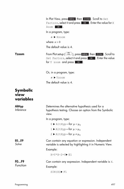
Programming 497
In Plot View, press then . Scroll to Set Factors,select it and press . Enter the value for X Zoom .
In a program, type:
Xzoom
where
The default value is 4.
Yzoom From Plot setup (P), press then . Scroll to Set Factors,select it and press . Enter the value for Y zoom and press .
Or, in a program, type:
Yzoom
The default value is 4.
Symbolic view variables
AltHypInference
Determines the alternative hypothesis used for a hypothesis testing. Choose an option from the Symbolic view.
In a program, type:
0 AltHyp—for
1 AltHyp—for
2 AltHyp—for
E0...E9Solve
Can contain any equation or expression. Independent variable is selected by highlighting it in Numeric View.
Example:
X+Y*X-2=Y E1
F0...F9Function
Can contain any expression. Independent variable is X.
Example:
SIN(X) F1
n
n 0
n
0
0
0

498 Programming
H1...H5Statistics 1Var
Contains the data values for a 1-variable statistical analysis. For example, H1(n) returns the nth value in the data set for the H1 analysis.
H1Type...H5TypeStatistics 1Var
Sets the type of plot used to graphically represent the statistical analyses H1 through H5. From the Symbolic setup, specify the type of plot in the field for Type1, Type 2, etc.
Or in a program, store one of the following constant integers or names into the variables H1Type, H2Type, etc.
0 Histogram (default)
1 Box and Whisker
2 Normal Probability
3 Line
4 Bar
5 Pareto
Example:
2H3Type
MethodInference
Determines whether the Inference app is set to calculate hypothesis test results or confidence intervals.
In a program, type:
0 Method—for Hypothesis Test
1 Method—for Confidence Interval
R0...R9Polar
Can contain any expression. Independent variable is .
Example:
2*SIN(2* ) R1
S1...S5Statistics 2Var
Contains the data values for a 2-variable statistical analysis. For example, S1(n) returns the nth data pair in the data set for the S1 analysis. With no argument, returns a list containing the independent column name, the dependent column name and the number of the fit type.

Programming 499
S1Type...S5TypeStatistics 2Var
Sets the type of fit to be used by the FIT operation in drawing the regression line. From Symbolic Setup view, specify the fit in the field for Type1,Type2, etc.
In a program, store one of the following constant integers or names into a variable S1Type,S2Type, etc.
0 Linear
1 Logarithmic
2 Exponential
3 Power
4 Exponent
5 Inverse
6 Logistic
7 Quadratic
8 Cubic
9 Quartic
10 User Defined
Example:
Cubic S2type
or
8 S2type
TypeInference
Determines the type of hypothesis test or confidence interval. Depends upon the value of the variable Method. Make a selection from the Symbolic view.
Or, in a program, store the constant number from the list below into the variable Type. With Method=0, the constant values and their meanings are as follows:
0 Z-Test:1
1 Z-Test:
2 Z-Test:1
3 Z-Test:
4 T-Test:1
5 T-Test:
With Method=1, the constants and their meanings are:
1 2–
1 2–
1 2–

500 Programming
0 Z-Int:1
1 Z-Int:
2 Z-Int:1
3 Z-Int:
4 T-Int:1
5 T-Int:
X0, Y0...X9,Y9Parametric
Can contain any expression. Independent variable is T.
Example:
SIN(4*T) Y1;2*SIN(6*T) X1
U0...U9Sequence
Can contain any expression. Independent variable is N.
Example:
RECURSE (U,U(N-1)*N,1,2) U1
Numeric view variables
C0...C9Statistics 2Var
C0 through C9, for columns of data. Can contain lists.
Enter data in the Numeric view.
In a program, type:
LIST Cn
where , 1, 2, 3 ... 9 and LIST is either a list or the name of a list.
D0...D9Statistics 1Var
D0 through D9, for columns of data. Can contain lists.
Enter data in the Numeric view.
In a program, type:
LIST Dn
where , 1, 2, 3 ... 9 and LIST is either a list or the name of a list.
1 2–
1 2–
1 2–
n 0=
n 0=
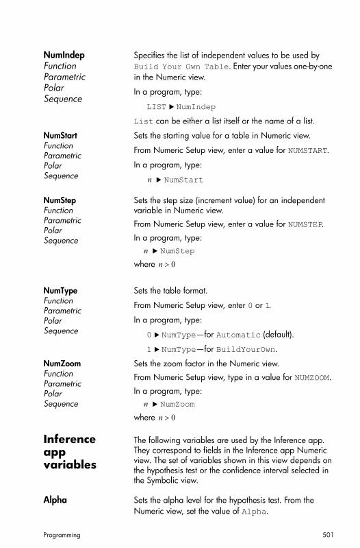
Programming 501
NumIndepFunctionParametricPolarSequence
Specifies the list of independent values to be used by Build Your Own Table. Enter your values one-by-one in the Numeric view.
In a program, type:
LIST NumIndep
List can be either a list itself or the name of a list.
NumStartFunctionParametricPolarSequence
Sets the starting value for a table in Numeric view.
From Numeric Setup view, enter a value for NUMSTART.
In a program, type:
NumStart
NumStepFunctionParametricPolarSequence
Sets the step size (increment value) for an independent variable in Numeric view.
From Numeric Setup view, enter a value for NUMSTEP.
In a program, type: NumStep
where
NumTypeFunctionParametricPolarSequence
Sets the table format.
From Numeric Setup view, enter 0 or 1.
In a program, type:
0 NumType—for Automatic (default).
1 NumType—for BuildYourOwn.
NumZoomFunctionParametricPolarSequence
Sets the zoom factor in the Numeric view.
From Numeric Setup view, type in a value for NUMZOOM.
In a program, type: NumZoom
where
Inference app variables
The following variables are used by the Inference app. They correspond to fields in the Inference app Numeric view. The set of variables shown in this view depends on the hypothesis test or the confidence interval selected in the Symbolic view.
Alpha Sets the alpha level for the hypothesis test. From the Numeric view, set the value of Alpha.
n
n
n 0
n
n 0

502 Programming
In a program, type:
Alpha
where
Conf Sets the confidence level for the confidence interval. From the Numeric view, set the value of Conf.
In a program, type:
Conf
where
Mean1 Sets the value of the mean of a sample for a 1-mean hypothesis test or confidence interval. For a 2-mean test or interval, sets the value of the mean of the first sample. From the Numeric view, set the value of Mean1.
In a program, type:
Mean1
Mean2 For a 2-mean test or interval, sets the value of the mean of the second sample. From the Numeric view, set the value of Mean2.
In a program, type:
Mean2
The following variables are used to set up hypothesis test or confidence interval calculations in the Inference app.
Sets the assumed value of the population mean for a hypothesis test. From the Numeric view, set the value of
.
In a program, type:
where
n1 Sets the size of the sample for a hypothesis test or confidence interval. For a test or interval involving the difference of two means or two proportions, sets the size of the first sample. From the Numeric view, set the value of n1.
In a program, type:
n
0 n 1
n
0 n 1
n
n
0
0
n 0
0 0 1

Programming 503
n1
n2 For a test or interval involving the difference of two means or two proportions, sets the size of the second sample. From the Numeric view, set the value of n2.
In a program, type:
n2
Sets the assumed proportion of successes for the One-proportion Z-test. From the Numeric view, set the value of
.
In a program, type:
where
Pooled Determine whether or not the samples are pooled for tests or intervals using the Student’s T-distribution involving two means. From the Numeric view, set the value of Pooled.
In a program, type:
0 Pooled—for not pooled (default).
1 Pooled—for pooled.
s1 Sets the sample standard deviation for a hypothesis test or confidence interval. For a test or interval involving the difference of two means or two proportions, sets the sample standard deviation of the first sample. From the Numeric view, set the value of s1.
In a program, type:
s1
s2 For a test or interval involving the difference of two means or two proportions, sets the sample standard deviation of the second sample. From the Numeric view, set the value of s2.
In a program, type:
s2
1 Sets the population standard deviation for a hypothesis test or confidence interval. For a test or interval involving
n
n
0
0
n 0
0 0 1
n
n
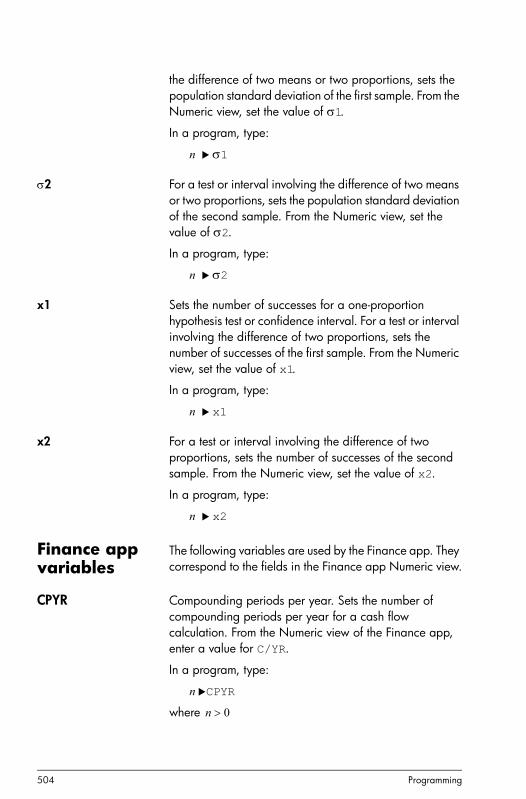
504 Programming
the difference of two means or two proportions, sets the population standard deviation of the first sample. From the Numeric view, set the value of 1.
In a program, type:
1
2 For a test or interval involving the difference of two means or two proportions, sets the population standard deviation of the second sample. From the Numeric view, set the value of 2.
In a program, type:
2
x1 Sets the number of successes for a one-proportion hypothesis test or confidence interval. For a test or interval involving the difference of two proportions, sets the number of successes of the first sample. From the Numeric view, set the value of x1.
In a program, type:
x1
x2 For a test or interval involving the difference of two proportions, sets the number of successes of the second sample. From the Numeric view, set the value of x2.
In a program, type:
x2
Finance app variables
The following variables are used by the Finance app. They correspond to the fields in the Finance app Numeric view.
CPYR Compounding periods per year. Sets the number of compounding periods per year for a cash flow calculation. From the Numeric view of the Finance app, enter a value for C/YR.
In a program, type:
CPYR
where
n
n
n
n
n
n 0

Programming 505
END Determines whether interest is compounded at the beginning or end of the compounding period. From the Numeric view of the Finance app. Check or uncheck END.
In a program, type:
1END—for compounding at the end of the period (Default)
0END—for compounding at the beginning of the period
FV Future value. Sets the future value of an investment. From the Numeric view of the Finance app, enter a value for FV.
In a program, type:
FV
Note: positive values represent return on an investment or loan.
IPYR Interest per year. Sets the annual interest rate for a cash flow. From the Numeric view of the Finance app, enter a value for I%YR.
In a program, type:
IPYR
where
NbPmt Number of payments. Sets the number of payments for a cash flow. From the Numeric view of the Finance app, enter a value for N.
In a program, type:
NbPmt
where
PMT Payment value. Sets the value of each payment in a cash flow. From the Numeric view of the Finance app, enter a value for PMT.
In a program, type:
PMT
Note that payment values are negative if you are making the payment and positive if you are receiving the payment.
n
n
n 0
n
n 0
n

506 Programming
PPYR Payments per year. Sets the number of payments made per year for a cash flow calculation. From the Numeric view of the Finance app, enter a value for P/YR.
In a program, type:
PPYR
where
PV Present value. Sets the present value of an investment. From the Numeric view of the Finance app, enter a value for PV.
In a program, type:
PV
Note: negative values represent an investment or loan.
GSize Group size. Sets the size of each group for the amortization table. From the Numeric view of the Finance app, enter a value for Group Size.
In a program, type:
GSize
Linear Solver app variables
The following variables are used by the Linear Solver app. They correspond to the fields in the app's Numeric view.
LSystem Contains a 2x3 or 3x4 matrix which represents a 2x2 or 3x3 linear system. From the Numeric view of the Linear Solver app, enter the coefficients and constants of the linear system.
In a program, type:
matrixLSystem
where matrix is either a matrix or the name of one of the matrix variables M0-M9.
Size Contains the size of the linear system. From the Numeric view of the Linear Solver app, press or .
In a program, type:
2Size—for a 2x2 linear system
3Size—for a 3x3 linear system
n
n 0
n
n

Programming 507
Triangle Solver app variables
The following variables are used by the Triangle Solver app. They correspond to the fields in the app's Numeric view.
SideA The length of Side A. Sets the length of the side opposite the angle A. From the Triangle Solver Numeric view, enter a positive value for A.
In a program, type:
SideA
where
SideB The length of Side B. Sets the length of the side opposite the angle B. From the Triangle Solver Numeric view, enter a positive value for B.
In a program, type:
SideB
where
SideC The length of Side C. Sets the length of the side opposite the angle C. From the Triangle Solver Numeric view, enter a positive value for C.
In a program, type:
SideC
where
AngleA The measure of angle . Sets the measure of angle . The value of this variable will be interpreted according to the angle mode setting (Degrees or Radians). From the Triangle Solver Numeric view, enter a positive value for angle
In a program, type:
AngleA
where
AngleB The measure of angle . Sets the measure of angle . The value of this variable will be interpreted according to the angle mode setting (Degrees or Radians). From the Triangle Solver Numeric view, enter a positive value for angle .
n
n 0
n
n 0
n
n 0
n
n 0

508 Programming
In a program, type:
AngleB
where
AngleC The measure of angle . Sets the measure of angle . The value of this variable will be interpreted according to the angle mode setting (Degrees or Radians). From the Triangle Solver Numeric view, enter a positive value for angle .
In a program, type:
AngleC
where
RECT Corresponds to the status of in the Numeric view of the Triangle Solver app. Determines whether a general triangle solver or a right triangle solver is used. From the Triangle Solver view, tap .
In a program, type:
0RECT—for the general Triangle Solver
1RECT—for the right Triangle Solver
Modes variables
The following variables are found in the Home Modes input form. They can all be over-written in an app's Symbolic setup.
Ans Contains the last result calculated in the Home view.
HAngle Sets the angle format for the Home view. From Modes view, choose Degrees or Radians for angle measure. In a program, type:
0 HAngle—for Degrees.
1 HAngle—for Radians.
HDigits Sets the number of digits for a number format other than Standard in the Home view. From the Modes view, enter a value in the second field of Number Format.
In a program, type:
n HDigits, where .
n
n 0
n
n 0
0 n 11

Programming 509
HFormat Sets the number display format used in the Home view. From the Modes view, choose Standard, Fixed, Scientific, or Engineering in the Number Format field.
In a program, store one of the following the constant numbers (or its name) into the variable HFormat:
0 Standard
1 Fixed
2 Scientific
3 Engineering
HComplex Sets the complex number mode for the Home view. From Modes, check or uncheck the Complex field. Or, in a program, type:
0 HComplex—for OFF.
1 HComplex—for ON.
Date Returns the system date. The format is YYYY.MMDD. This format is used irrespective of the format set on the Home Settings screen.
Time Returns the system time or sets the system time.
HHMMSS Time
Language Sets the language. From Modes, choose a language for the Language field.
In a program, store one of the following constant numbers into the variable Language:
1 Language (English)
2 Language (Chinese)
3 Language (French)
4 Language (German)
5 Language (Spanish)
6 Language (Dutch)
7 Language (Portuguese)
Entry Sets the entry mode. In a program, enter:
0 Entry—for Textbook

510 Programming
1 Entry—for Algebraic
2 Entry—for RPN
Integer
Base Returns or sets the integer base. In a program, enter:
0 Base—for Binary
1 Base—for Octal
2 Base—for Decimal
3 Base—for Hexadecimal
Bits Returns or sets the number of bits for representing integers. In a program, enter:
n Bits where n is the number of bits.
Signed Returns or sets a flag indicating that the integer wordsize is signed or not. In a program, enter:
0 Signed—for unsigned
1 Signed—for signed
The following variables are found in the Symbolic setup of an app. They can be used to overwrite the value of the corresponding variable in Home Modes.
AAngle Sets the angle mode.
From Symbolic setup, choose System, Degrees, or Radians for angle measure. System (default) will force the angle measure to agree with that in Modes.
In a program, type:
0 AAngle—for System (default).
1 AAngle—for Degrees.
2 AAngle—for Radians.
AComplex Sets the complex number mode.
From Symbolic setup, choose System, ON, or OFF. System (default) will force this setting to agree with the corresponding setting in Home Modes.
In a program, type:

Programming 511
0 AComplex—for System (default).
1 AComplex—for ON.
2 AComplex—for OFF.
ADigits Defines the number of decimal places to use for the Fixed number format in the app’s Symbolic Setup. Affects results in the Home view.
From Symbolic setup, enter a value in the second field of Number Format.
In a program, type:
ADigits
where
AFormat Defines the number display format used for number display in the Home view and to label axes in the Plot view.
From Symbolic setup, choose Standard, Fixed, Scientific, or Engineering in the Number Format field.
In a program, store the constant number (or its name) into the variable AFormat.
0 System
1 Standard
2 Fixed
3 Scientific
4 Engineering
Example:
Scientific AFormat
or3 AFormat
Results variables
The Function, Linear Solver, Statistics 1Var, Statistics 2Var, and Inference apps offer functions that generate results that can be re-used outside those apps (such as in a program). For example, the Function app can find a root of a function, and that root is written to a variable called Root. That variable can then be used elsewhere.
n
0 n 11

512 Programming
The results variables are listed with the apps that generate them. See “App variables” on page 378.

Integer arithmetic 513
27
Integer arithmetic
The common number base used in contemporary mathematics is base 10. By default, all calculations performed by the HP Prime are carried out in base 10, and all results are displayed in base 10.
However, the HP Prime enables you to carry out integer arithmetic in four bases: decimal (base 10), binary, (base 2), octal (base 8), and hexadecimal (base 16). For example, you could multiply 4 in base 16 by 71 in base 8 and the answer is E4 in base 16. This is equivalent in base 10 to multiplying 4 by 57 to get 228.
You indicate that you are about to engage in integer arithmetic by preceding the number with the pound symbol (#, got by pressing Az). You indicate what base to use for the number by appending to the appropriate base marker:
Thus #11b represents 310. The base marker b indicates that the number is to interpreted as a binary number: 112. Likewise #E4h
Base marker Base
[blank] Adopt the defualt base (see “The default base” on page 514)
d decimal
b binary
o octal
h hexadecimal

514 Integer arithmetic
represents 22810. In this case, the base marker h indicates that the number is to interpreted as a hexadecimal number: E416.
Note that with integer arithmetic, the result of any calculation that would return a remainder in floating-point arithmetic is truncated: only the integer portion is presented. Thus #100b/#10b gives the correct answer: #10b (since 410/210 is 210). However, #100b/#11b gives just the integer component of the correct result: #1b.
Note too that the accuracy of integer arithmetic can be limited by the integer wordsize. The wordsize is the maximum number of bits that can represent an integer. You can set this to any value between 1 and 64. The smaller the wordsize, the smaller the integer that can be accurately represented. The default wordsize is 32, which is adequate for representing integers up to approximately 2 × 10⁹. However, integers larger than that would be truncated, that is, the most significant bits (that is, the leading bits) would be dropped. thus the result of any calculation involving such a number would not be accurate.
The default baseSetting a default base only affects the entry and display of numbers being used in integer arithmetic. If you set the default base to binary, 27 and 44 will still be represented that way in Home view, and result of those numbers being added will still be represented as 71. However, if you entered #27b, you would get a syntax error, as 2 and 7 are not integers found in binary arithmetic. You would have to enter 27 as #11011b (since 2710=110112).
Setting a default base means that you do not always have to specify a base marker for numbers when doing integer arithmetic. The exception is if you want to include a number from the non-default base: it will have to include the base marker. Thus if your default base is 2 and you want to enter 27 for an integer arithmetic operation, you could enter just #11011 without the b suffix. But if you wanted to enter E416, you need to enter it with the suffix: #E4h. (The HP Prime adds any omitted base markers when the calculation is displayed in history.)
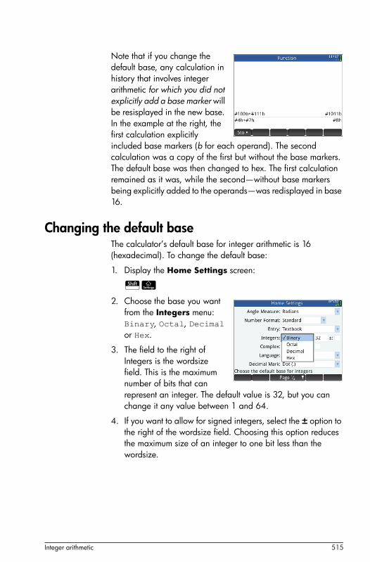
Integer arithmetic 515
Note that if you change the default base, any calculation in history that involves integer arithmetic for which you did not explicitly add a base marker will be resisplayed in the new base. In the example at the right, the first calculation explicitly included base markers (b for each operand). The second calculation was a copy of the first but without the base markers. The default base was then changed to hex. The first calculation remained as it was, while the second—without base markers being explicitly added to the operands—was redisplayed in base 16.
Changing the default baseThe calculator’s default base for integer arithmetic is 16 (hexadecimal). To change the default base:
1. Display the Home Settings screen:
SH
2. Choose the base you want from the Integers menu: Binary, Octal, Decimal or Hex.
3. The field to the right of Integers is the wordsize field. This is the maximum number of bits that can represent an integer. The default value is 32, but you can change it any value between 1 and 64.
4. If you want to allow for signed integers, select the ± option to the right of the wordsize field. Choosing this option reduces the maximum size of an integer to one bit less than the wordsize.
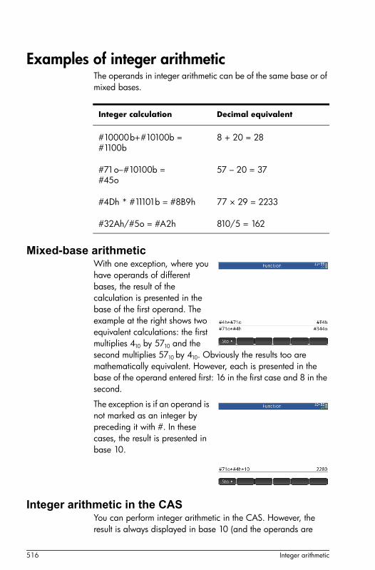
516 Integer arithmetic
Examples of integer arithmeticThe operands in integer arithmetic can be of the same base or of mixed bases.
Mixed-base arithmeticWith one exception, where you have operands of different bases, the result of the calculation is presented in the base of the first operand. The example at the right shows two equivalent calculations: the first multiplies 410 by 5710 and the second multiplies 5710 by 410. Obviously the results too are mathematically equivalent. However, each is presented in the base of the operand entered first: 16 in the first case and 8 in the second.
The exception is if an operand is not marked as an integer by preceding it with #. In these cases, the result is presented in base 10.
Integer arithmetic in the CASYou can perform integer arithmetic in the CAS. However, the result is always displayed in base 10 (and the operands are
Integer calculation Decimal equivalent
#10000b+#10100b = #1100b
8 + 20 = 28
#71o–#10100b = #45o
57 – 20 = 37
#4Dh * #11101b = #8B9h 77 × 29 = 2233
#32Ah/#5o = #A2h 810/5 = 162
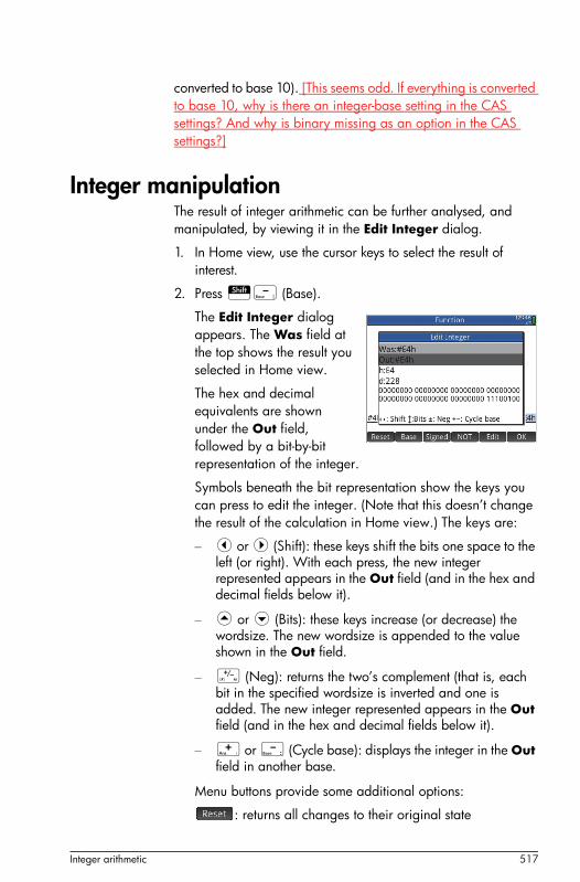
Integer arithmetic 517
converted to base 10). [This seems odd. If everything is converted to base 10, why is there an integer-base setting in the CAS settings? And why is binary missing as an option in the CAS settings?]
Integer manipulationThe result of integer arithmetic can be further analysed, and manipulated, by viewing it in the Edit Integer dialog.
1. In Home view, use the cursor keys to select the result of interest.
2. Press Sw (Base).
The Edit Integer dialog appears. The Was field at the top shows the result you selected in Home view.
The hex and decimal equivalents are shown under the Out field, followed by a bit-by-bit representation of the integer.
Symbols beneath the bit representation show the keys you can press to edit the integer. (Note that this doesn’t change the result of the calculation in Home view.) The keys are:
– < or > (Shift): these keys shift the bits one space to the left (or right). With each press, the new integer represented appears in the Out field (and in the hex and decimal fields below it).
– = or \ (Bits): these keys increase (or decrease) the wordsize. The new wordsize is appended to the value shown in the Out field.
– Q (Neg): returns the two’s complement (that is, each bit in the specified wordsize is inverted and one is added. The new integer represented appears in the Out field (and in the hex and decimal fields below it).
– + or w (Cycle base): displays the integer in the Out field in another base.
Menu buttons provide some additional options:
: returns all changes to their original state
518 Integer arithmetic
: cycles through the bases; same as pressing +
: toggles the wordsize between signed and unsigned
: returns the one’s complement (that is, each bit in the specified wordsize is inverted: a 0 is replaced by 1 and a 1 by 0. The new integer represented appears in the Out field (and in the hex and decimal fields below it).
: activates edit mode. A cursor appear sand you can move abut the dialog using the cursor keys. The hex and decimal fields can be modified, as can the bit representation. A change in one such field automatically modifies the other fields.
: closes the dialog and saves your changes. If you don’t want to save your changes, press J instead.
3. Make whatever changes you want.
4. To save your changes, tap ; otherwise press J.
N o t e If you save changes, the next time you select that same result in Home view and open the Edit Integer dialog, the value shown in the Was field will be the value you saved, not the value of the result.
Base functionsNumerous functions related to integer arithmetic can be invoked from Home view, CAS view, and within programs:
These are described in “Integer”, beginning on page 483.
• BITAND • BITNOT • BITOR
• BITSL • BITSR • BITXOR
• B→R • GETBASE • GETBITS
• R→B • SETBASE • SETBITS

Limiting functionality 519
28
Limiting functionality
Certain functions of the calculator can be disabled for a set period, with the disabling controlled by a password. This feature will primarily be of interest to teachers, proctors, and invigilators who want to ensure that the calculator is used appropriately by students sitting an examination. In the illustration above, user-customized apps, the help system and the computer algebra system have been selected for disabling.
The settings, and a list of the functions that can be disabled, are accessible from the Home Settings screen. When you disable functions, you put the calculator into exam mode.
Before initiating exam mode, you can choose to activate a light on the calculator that will flash periodically during exam mode. The light is on the top edge of the calculator. The light will help the supervisor of the examination detect if any particular calculator has dropped out of exam mode. (The flashing of lights on all calculators placed in exam mode will be synchronised so that all will flash at the same time.)
Exam configurationsA particular set of enabled and disabled functions is called an exam mode configuration. You can create a default exam mode configuration. You can also create any number of additional configurations (each with a name of your choosing).

520 Limiting functionality
A configuration named Default Exam appears when you first access the Exam Mode screen. This configuration has no functions disabled. If only one configuration is needed, you can simply modify the default exam configuration. If you envisage the need for a number of configurations—different ones for different examinations, for example—modify the default configuration so that it matches the settings you will most often need, and then create other configurations for the settings you will need less often.
There are two ways to access the screen for configuring and activating exam mode:
• press O + A + c
• choose the third page of the Home Settings screen.
The procedure below illustrates the second method.
Modifying the default configuration1. Press SH. The Home Settings screen appears.
2. Tap .
3. Tap .
The Exam Mode screen appears. You use this screen to activate a particular configuration (just before an examination begins, for example).
4. Tap . The Exam Mode Configuration screen appears.
5. Select those functions you want disabled, and make sure that those functions you don’t want disabled are not selected.

Limiting functionality 521
An expand box at the left of a function indicates that there are sub-functions that you can individually disable. (Notice that there is an expand box beside System Apps in the example shown above.) Tap on the expand box to see the sub-functions. You can then select the sub-functions individually. If you want to disable all the sub-functions, just select the top-level function.
You can select (or deselect) an option either by tapping on the check box beside it, or by using the cursor keys to scroll to it and tapping .
6. When you have finished selecting the functions to be disabled, tap .
If you want to activate exam mode now, continue with “Activating Exam Mode” below.
To return to the default configuration
1. Press SH. The Home Settings screen appears.
2. Tap .
3. Tap .
The Exam Mode screen appears.
4. Choose Default Exam from the Configuration list.
5. Tap , select Reset from the menu and tap to confirm your intention to return the
configuration to its default settings.
Creating a new configurationYou can modify the default exam configuration when new circumstances require a different set of disabled functions. Alternatively, you can retain the default configuration and create a new configuration. When you create a new configuration, you choose an existing configuration on which to base it.
1. Press SH. The Home Settings screen appears.

522 Limiting functionality
2. Tap .
3. Tap .
The Exam Mode screen appears.
4. Choose a base configuration from the Configuration list. If you have not created any exam mode configurations before, the only base configuration will be Default Exam.
5. Tap , select Copy from the menu and enter a name for the new configuration.
See “Adding text” on page 20 if you need help with entering alphabetic characters.
6. Tap twice.
7. Tap . The Exam Mode Configuration screen appears.
8. Select those functions you want disabled, and make sure that those functions you don’t want disabled are not selected.
9. When you have finished selecting the functions to be disabled, tap .
If you want to activate exam mode now, continue with “Activating Exam Mode” below.
Activating Exam ModeWhen you activate exam mode you prevent users of the calculator from accessing those features you have disabled. The features become accessible again at the end of the specified time-out period or on entry of the exam-mode password, whichever occurs sooner.
To activate exam mode:

Limiting functionality 523
1. tIf the Exam Mode screen is not showing, press SH, tap
and tap .
2. If a configuration other than Default Exam is required, choose it from the Configuration list.
3. Select a time-out period from the Timeout list.
Note that 8 hours is the maximum period. If you are preparing to supervise a student examination, make sure that the time-out period chosen is greater than the duration of the examination.
4. Enter a password of between 1 and 10 characters. The password must be entered if you—or another user—wants to cancel exam mode before the time-out period has elapsed.
5. If you want to erase the memory of the calculator, select Erase memory. This will erase all user entries and return the calculator to its factory default settings.
6. If you want the exam mode indicator to flash periodically while the calculator is in exam mode, select Blink LED.
7. Using the supplied USB cable, connect a student’s calculator.
Insert the micro-A connector—the one with the rectangular end—into the USB port on the sending calculator, and the other connector into the USB port on the receiving calculator.
8. To activate the configuration on an attached calculator, tap . The Exam Mode screen closes. The connected calculator is now in exam mode, with the specified disabled features not accessible to the user of that calculator.

524 Limiting functionality
9. Repeat from step 7 for each calculator that needs to have its functionality limited.
Cancelling exam modeIf you want to cancel exam mode before the set time period has elapsed, you will need to enter the password for the current exam mode activation.
1. Connect the calculator that is in exam mode.
2. If the Exam Mode screen is not showing, press SH, tap and tap .
3. Enter the password for the current exam mode activation and tap twice.
Modifying configurationsExam mode configurations can be changed. You can also restore the default configuration.
To change a configuration1. If the Exam Mode screen is not showing, press
SH, tap and tap .
2. Select the configuration you want to change from the Configuration list.
3. Tap .
4. Make whatever changes are necessary and then tap .
Deleting configurationsYou cannot delete the default exam configuration (even if you have modified it). You can only delete those that you have created. To delete a configuration:
1. If the Exam Mode screen is not showing, press SH, tap and tap .
2. Select the configuration you want to delete from the Configuration list.

Limiting functionality 525
3. Tap and choose Delete.
4. When asked to confirm the deletion, tap or press E.

526 Limiting functionality
527
Appendix A
Glossary
app A small application, designed for the study of one or more related topics or to solve problems of a particular type. The built-in apps are Geometry, Function, Solve, Statistics 1Var, Statistics 2Var, Inference, Parametric, Polar, Sequence, Finance, Linear Solver, Triangle Solver, Linear Explorer, Quadratic Explorer, Trig Explorer, Spreadsheet, Advanced Graphing and Datastreamer. An app can be filled with the data and solutions for a specific problem. It is reusable (like a program, but easier to use) and it records all your settings and definitions.
button An option or menu shown at the bottom of the screen and activated by touch. Compare with key.
CAS Computer Algebra System. Use the CAS to perform calculations in symbolic mode. Such calculations always return exact answers (unlike calculations done in Home view, which yield numeric approximations). You can share results and variables between the CAS and Home view (and vice versa).
catalog A collection of items, such as matrices, lists, programs and the like. New items you create are saved to a catalog, and you choose a specific item from a catalog to work on it. A special catalog that lists the apps is called the Application Library.

528
command An operation for use in programs. Commands can store results in variables, but do not display results.
expression A number, variable, or algebraic expression (numbers plus functions) that produces a value.
function An operation, possibly with arguments, that returns a result. It does not store results in variables. The arguments must be enclosed in parentheses and separated with commas.
Home view The basic starting point of the calculator. Most calculations can be done in Home view. However, such calculations only return numeric approximations. For exact results, you can use the CAS. You can share results and variables between the CAS and Home view (and vice versa).
input form A screen where you can set values or choose options. Another name for a dialog box.
key A key on the keypad (as opposed to a button, which appears on the screen and needs to be tapped to be activated).
Library A collection of items, more speficially, the the apps. See also catalog.
list A set of values separated by commas and enclosed in braces. Lists are commonly used to enter statistical data and to evaluate a function with multiple values. Created and manipulated by the List Editor and.
matrix A two-dimensional array of values separated by commas and enclosed in nested square brackets. Created and manipulated by the Matrix Editor. Vectors are also handled by the Matrix Editor.

529
menu A choice of options given in the display. It can appear as a list or as a set of touch buttons across the bottom of the display.
note Text that you write in the Note Editor. It can be a general, standalone note or a note specific to an app.
program A reusable set of instructions that you record using the Program Editor.
variable A name given to an object—such as a number, list, matrix, graphic and so on—to assist in later retrieving it. The
command assigns a variable, and the object can be retrieved by selecting the associated variable from the variables menu (a).
vector A one-dimensional array of values separated by commas and enclosed in single square brackets. Created and manipulated by the Matrix Editor.
views The six primary environments for creating and manipulating apps: Plot, Plot Setup, Numeric, Numeric Setup, Symbolic, and Symbolic Setup.

530

531
Appendix B
Troubleshooting
Calculator not respondingIf the calculator does not respond, you should first try to reset it. This is much like restarting a PC. It cancels certain operations, restores certain conditions, and clears temporary memory locations. However, it does not clear stored data (variables, apps, programs, etc.).
To resetPress and hold O and Y simultaneously, and then release them.
If this doesn’t work, you should restore factory settings (see below).
To restore factory settingsIf the calculator does not respond to a reset (see above), you should restore factory settings. This will entirely erase the calculator’s memory. You will lose everything you have stored.
1. Press and hold O then I and then J.
2. Release all keys in the reverse order.
If the calculator does not turn on
If the HP Prime does not turn on, follow the steps below until the calculator turns on. You may find that the calculator turns on before you have completed the procedure. If the calculator still does not turn on, contact Customer Support for further information.
1. Press and hold O for 10 seconds, then release.

532
2. Press and hold Oand ?simultaneously, then release?, then release O.
3. Press and holdO,?,and? simultaneously. Release ?, then release ?, and then release O.
4. Remove the batteries, press and hold Ofor 10 seconds, then put the batteries back in and press O.
Operating limitsOperating temperature: 0 to 45C (32 to 113F).
Storage temperature: –20 to 65C (– 4 to 149F).
Operating and storage humidity: 90% relative humidity at 40C (104F) maximum. Avoid getting the calculator wet.
Battery operates at 6.0V dc, 80mA maximum.
Status messagesMessage Meaning
Bad Argument Type
Incorrect input for this operation.
Bad Argument Value
The value is out of range for this operation.
Infinity error Math exception, such as 1/0.
Insufficient Memory
You must recover some memory to continue operation. Delete one or more customized apps, matrices, lists, notes, or programs.
Insufficient Statistics Data
Not enough data points for the calculation. For two-variable statistics there must be two columns of data, and each column must have at least four numbers.

533
Invalid Dimension Array argument had wrong dimensions.
Invalid Statistics Data
Need two columns with equal numbers of data values.
Invalid Syntax The function or command you entered does not include the proper arguments or order of arguments. The delimiters (parentheses, commas, periods, and semi-colons) must also be correct. Look up the function name in the index to find its proper syntax.
Name Conflict The | (where) function attempted to assign a value to the variable of integration or summation index.
No equations checked
You must enter and check an equation in the Symbolic view before entering the Plot view.
Receive Error Problem with data reception from another calculator. Re-send the data.
Too Few Arguments
The command requires more arguments than you supplied.
Undefined Name The global variable named does not exist.
Undefined Result The calculation has a mathematically undefined result (such as 0/0).
Out of Memory You must recover a lot of memory to continue operation. Delete one or more customized apps, matrices, lists, notes, or programs.
Message Meaning (Continued)

534

Product Regulatory Information 535
Appendix C
Product Regulatory Information
Federal Communications Commission NoticeThis equipment has been tested and found to comply with the limits for a Class B digital device, pursuant to Part 15 of the FCC Rules. These limits are designed to provide reasonable protection against harmful interference in a residential installation. This equipment generates, uses, and can radiate radio frequency energy and, if not installed and used in accordance with the instructions, may cause harmful interference to radio communications. However, there is no guarantee that interference will not occur in a particular installation. If this equipment does cause harmful interference to radio or television recep-tion, which can be determined by turning the equipment off and on, the user is encouraged to try to correct the interference by one or more of the following measures:
• Reorient or relocate the receiving antenna.• Increase the separation between the equipment and the
receiver.• Connect the equipment into an outlet on a circuit different
from that to which the receiver is connected.• Consult the dealer or an experienced radio or television
technician for help.
ModificationsThe FCC requires the user to be notified that any changes or modifications made to this device that are not expressly approved by Hewlett-Packard Company may void the user's authority to operate the equipment.
CablesConnections to this device must be made with shielded cables with metallic RFI/EMI connector hoods to main-tain compliance with FCC rules and regulations. Applica-ble only for products with connectivity to PC/laptop.
Declaration of Conformity for products Marked with FCC

536 Product Regulatory Information
Logo, United States OnlyThis device complies with Part 15 of the FCC Rules. Oper-ation is subject to the following two conditions: (1) this device may not cause harmful interference, and (2) this device must accept any interference received, including interference that may cause undesired operation.
If you have questions about the product that are not related to this declaration, write to:Hewlett-Packard CompanyP.O. Box 692000, Mail Stop 530113Houston, TX 77269-2000
For questions regarding this FCC declaration, write to:Hewlett-Packard CompanyP.O. Box 692000, Mail Stop 510101 Houston, TX 77269-2000 or call HP at 281-514-3333
To identify your product, refer to the part, series, or model number located on the product.
Canadian NoticeThis Class B digital apparatus meets all requirements of the Canadian Interference-Causing Equipment Regula-tions.
Avis CanadienCet appareil numérique de la classe B respecte toutes les exigences du Règlement sur le matériel brouilleur du Can-ada.

Product Regulatory Information 537
European Union Regulatory NoticeProducts bearing the CE marking comply with the follow-ing EU Directives:
• Low Voltage Directive 2006/95/EC• EMC Directive 2004/108/EC• Ecodesign Directive 2009/125/EC, where applicable
CE compliance of this product is valid if powered with the correct CE-marked AC adapter provided by HP. Compliance with these directives implies conformity to applicable harmonized European standards (European Norms) that are listed in the EU Declaration of Confor-mity issued by HP for this product or product family and available (in English only) either within the product docu-mentation or at the following web site: www.hp.eu/cer-tificates (type the product number in the search field).
The compliance is indicated by one of the following con-formity markings placed on the product:
Please refer to the regulatory label provided on the prod-uct.The point of contact for regulatory matters is:Hewlett-Packard GmbH, Dept./MS: HQ-TRE, Herren-berger Strasse 140, 71034 Boeblingen, GERMANY.
For non-telecommunications products and for EU harmonized telecommunications products, such as Bluetooth® within power class below 10mW.
For EU non-harmonized telecommunications products (If applicable, a 4-digit notified body number is inserted between CE and !).

538 Product Regulatory Information
Japanese Notice
Korean Class Notice
Disposal of Waste Equipment by Users in Private Household in the European Union
This symbol on the product or on its packaging indicates that this product must not be disposed of with your other household waste. Instead, it is your responsibility to dispose of your waste equipment by handing it over to a designated collection point for the recycling of waste electrical and electronic equipment. The separate collection and recycling of your waste equipment at the time of disposal will help to conserve natural resources and ensure that it is recycled in a manner that protects human health and the environment. For more information about where you can drop off your waste equipment for recycling, please contact your local city office, your household waste disposal service or the shop where you purchased the product.

Product Regulatory Information 539
Chemical Substances
HP is committed to providing our customers with informa-tion about the chemical substances in our products as needed to comply with legal requirements such as REACH (Regulation EC No 1907/2006 of the European Parliament and the Council). A chemical information report for this product can be found at:
http://www.hp.com/go/reach
Perchlorate Material - special handling may applyThis calculator's Memory Backup battery may contain perchlorate and may require special handling when recycled or disposed in California.

540 Product Regulatory Information
Index 541
Index
Aabsolute value 303add 299Advanced Graphing 197Advanced Graphing app vari-ables
summary 486algebraic entry 31angle measure 28annunciators 12Ans (last answer) 36antilogarithm
common 300natural 300
apletkey 17
aplet viewscanceling operations in 10
appattaching notes 296commands 410definition of 479delete 82deleting 297Explorer 217Finance 203Function 119functions 460HP Apps 79, 471Inference 167library 81Linear Solver 211open 81Parametric 187Polar 193reset 81resetting 296sending and receiving 296Sequence 199
sorting 81, 82sorting the app list 297Triangle Solver 213
app functions 502Common 468Finance 464Function 460Inference 464Linear Solver 466Statistics 1Var 462Statistics 2Var 463Triangle Solver 467
app variableslist of 484Mode 455Numeric view 445Plot view 437Results 456Symbolic view 441
app viewsSymbolic view 83
arc cosine 301arc sine 301arc tangent 301area
between curves 128arguments
conventions 355Bbackspace 18bad argument 510bar plot 149battery indicator 14block commands 412Boolean operators 18box-and-whisker plot 149branch commands 413butons
menu 17buttons
command 17

542 Index
Ccalculus functions 306CAS 479CAS variables 495catalog 479clearing
an app 296characters 34display 34
clonememory 381
cobweb graph 199coefficient of determination 163command button 17commands
app 410assignment 413block 412branch 413definition of 410, 480drawing 414I/O 422loop 426matrix 429string 431test 433variable 435
complex number 307complex number functions 307complex numbers 38
storing 39confidence interval 168confidence intervals 180constants 307–308
mathematical 307physical 331, 509program 508
context sensitive menu 17copying
display 35notes 369programs 396
correlation coefficient 163covariance 161critical value(s) displayed 170Ddata set definition 154DataStreamer 80debugging programs 394decimal
changing format 28default value, returning to 18define your own fit 160defining functions 325definite integral
definition of 306degree symbol 18delete 18delete an app 82deleting
lists 336matrices 346notes 364programs 386statistical data 146, 158
derivativesdefinition of 306
determinant 355display
annunciator line 12clearing 11engineering 28fixed 28fraction 28history 35line 35matrices 349one element in a list 338one element in a matrix 349parts of 12scientific 28soft key labels 12standard 28
divide 299

Index 543
DMS format 18drawing commands 414–421Eediting
lists 333matrices 346notes 363programs 385
editors 39Eigen values 356Eigen vectors 356element
storing 350engineering number format 28entry methods 31equations
definition of 133Explorer apps 217exponent
fit 159minus 1 313raising to 302
exponential 300expression
definition of 480extremum 130Ffactorial (!) 319Finance app 203Finance app variables
Numeric view 449–451summary 494
finding statistical values 343fixed number format 28flick 14format
hexagesimal 22fractions 37full-precision display 28function
definition of 480entering 32
syntax 306Function app 119Function app functions 460Function app variables
results 456summary 485
functionsapp 502area 128creating your own 325definition of 119intersection point 127Math menu 497slope 128tracing 122
GGeometry app variables
summary 485gestures 14glossary 479graph
bar 149box-and-whisker 149cobweb 199histogram 148line 149normal probability 149pareto 149stairsteps 199statistical data
one-variable 148graphics
copying into an app 369storing and recalling 414
Greek characters 18Hheader 12hexagesimal format 22histogram 148Home 11
calculating in 31reusing lines 35
544 Index
settings 27variables 371, 483variables categories 377
Home variableslist of 483
horizontal zoom 99, 111hyperbolic trig 56–??, 56–??,57–??, 312–313hypothesis
alternative hypothesis 168tests 168
II/O commands 422implied multiplication 33importing graphics 369inference
confidence intervals 180hypothesis tests 173One-Proportion Z-Interval 182One-Proportion Z-Test 175One-Sample T-Interval 184One-Sample T-Test 178One-Sample Z-Interval 180One-Sample Z-Test 173Two-Proportion Z-Interval 183Two-Proportion Z-Test 176Two-Sample T-Interval 184Two-Sample T-Test 179Two-Sample Z Test 174Two-Sample Z-Interval 181
Inference app variablesNumeric view 446Results 460summary 490
infinite result 510insufficient memory 510insufficient statistics data 510integer functions 313, ??–314,??–317integral
definite 306invalid
dimension 510statistics data 510syntax 510
inverse hyperbolic trig 312Kkey 480keyboard
customizing 403editing keys 17entry keys 17inactive keys 23list
catalog keys 335LLibrary 480line plot 149Linear Explorer app variables
summary 494linear fit 159Linear Solver
app 211Linear Solver app variables
Numeric view 451Results 457summary 494
listdeleting 336displaying one element 337editing 335evaluating 337functions 338list variables 333sending and receiving 338,
381storing one element 338syntax 339variables 333
logarithm 300logarithmic
fit 159functions 300
loop commands 426–429

Index 545
loop functions 317lowercase characters 366Mmantissa 322Math functions
calculus 306complex number 307distribution 308–312hyperbolic trig 312list 317logical operators 324loop 317Math menu summary 497on keyboard 299polynomial 318probability 319real-number 320test 324–??trigonometry 324
math functionsmenu 25
math operations 31enclosing arguments 33in scientific notation 22negative numbers in 33
math templates 21matrices
adding rows 347addition and subtraction 350arithmetic operations in 350column norm 355commands 429–431condition number 355create identity 359deleting 346deleting columns 347deleting rows 347determinant 355displaying 349displaying matrix elements
349dividing by a square matrix
352dot product 355functions 354–359inverting 352matrix calculations 345multiplying and dividing by
scalar 351multiplying by vector 351negating elements 353raised to a power 352sending or receiving 350singular value decomposition
359size 358storing matrix elements 350swap row 431transposing 360variables 345
maximum real number 34, 308memory
clearing all 482memory management 293out of 511saving 36viewing available memory
372menu
context sensitive 17menu button 17menu lists
searching 24menu shortcuts 24minimum real number 308minutes symbol 18mixed numbers 37modes
angle measure 28decimal mark 29number format 28
Modes app variables 455modes See settings 27multiplication 299
implied 33

546 Index
Nname conflict 510natural exponential 56, 300, 313natural log plus 1 313natural logarithm 300navigation 14negation 303negative numbers 33no equations checked 511normal probability plot 149Normal Z-distribution, confidenceintervals 180note
copying 368creating 364creating in an app 116, 365editing 365–369importing from note catalog
368nth root 302number format
engineering 28fixed 28scientific 28Standard 28
Numeric view app variables 436Ooff
automatic 11power 10
on/cancel 10One-Proportion Z-Interval 182One-Proportion Z-Test 175One-Sample T-Interval 184One-Sample T-Test 178One-Sample Z-Interval 180One-Sample Z-Test 173order of precedence 33P 308Parametric app 187
define the expression 188
exploring the graph 190parametric app variables 490parentheses
to close arguments 33to specify order of operation
33pareto plot 149permutations 319physical constants 331, 509pinch 15plot
box-and-whisker 149cobweb 199histogram 148line 149one-variable statistics 148pareto 149scatter 162stairsteps 199statistical data
one-variable 148two-variable 162
Plot view app variables 437–441Polar app 193Polar app variables 492power (x raised to y) 302precedence 34probability functions 319–320QQuadratic Explorer app variables
summary 495quadratic fit 160quotes in strings 431Rrandom numbers 320real number
maximum 308minimum 308
real-number functions 320–324receive error 511reduced-row echelon form 360regression 159

Index 547
reset app 81resetting
app 296calculator 481memory 482
resultcopying to edit line 35reusing 35
reverse polish notation, See RPN29root
nth 302RPN 29, 31, 41Sscientific number format 22, 28scrolling
move between relations inTrace mode 104
searchingmenu lists 24speed searches 24
seconds symbol 18sending
apps 296lists 338matrices 350notes 369programs 396
Sequence app 199graphs 199
Sequence app variablesin menu map 492
settingsHome 27
shortcutsmenus 24
Show button 33sign reversal 139sine 301sine cosine tangent 301Solve app function 462Solve app variables 486
summary 486sort apps 81, 82split-screen 116Spreadsheet app variables
summary 486square root 302stack 42stairsteps graph 199standard number format 28statistical data
two variable 162Statistics 1Var
data set definition 142deleting data 146, 158editing data 146, 158histogram
range 150width 150
inserting data 146, 158plot types 148sorting data 146, 158
Statistics 1Var app variablesResults 456summary 488
Statistics 2Varadjusting plotting scale 162choosing the fit 159curve fitting 159define your own fit 160defining a fit 159defining a regression model
159fit models 159, 160getting started 153inserting data 158plot setup 164predicted values 165regression curve (fit) models
159tracing a scatter plot 162troubleshooting plots 166
Statistics 2Var app variablesResults 458

548 Index
summary 489storing
a value in Home view 372list element 338matrix elements 350
subtract 299syntax of functions 306Ttangent 301template key 21templates 18textbok entry 31the 335time 13times sign 33too few arguments 511touch options 14tracing
more than one curve 104transmitting
lists 338matrices 350notes 369programs 396
Triangle Solver app 213Triangle Solver app functions 467Triangle Solver app variables
Numeric view 452summary 494
Trig Explorer app variablessummary 495
trigonometricfit 160functions 324
Two-Proportion Z-Interval 183Two-Proportion Z-Test 176Two-Sample T-Interval 184Two-Sample T-test 179Two-Sample Z-Interval 181Two-Sample Z-Test 174Uundefined
name 511result 511
uppercase characters 366Upper-Tail Chi-Square probability320Upper-Tail Normal Probability320Upper-Tail Snedecor’s F probabil-ity 320Upper-Tail Student’s t-probability320user defined
regression fit 160variables 399
user keyboard 403user variables 379, 495Vvalue
recall 374variable
definition of 481variables
App 436CAS 54, 374, 495categories 371, 377Home 377list of 483Modes 455Numeric view 445Plot view 437previous result (Ans) 35Results 456–460Symbolic view 441–444types of in programming 436use in calculations 374User 436user 495
variables user 379variables, shared 374Vars menu 374vectors
definition of 345, 481

Index 549
viewsdefinition of 481
Wwarning symbol 23Where command (|) 306ZZ-Intervals 180–183zoom
examples of 101