hrtf sound localization - intech - open science open minds

Martin Rothbucher, David Kronmüller, Marko Durkovic, Tim Habigt andKlaus Diepold

Institute for Data Processing, Technische Universität MünchenGermany

1. Introduction

In order to improve interactions between the human (operator) and the robot (teleoperator) inhuman centered robotic systems, e.g. Telepresence Systems as seen in Figure 1, it is importantto equip the robotic platform with multimodal human-like sensing, e.g. vision, haptic andaudition.

Operator Site Teleoperator Site

iers

Barr

i

Fig. 1. Schematic view of the telepresence scenario.

Recently, robotic binaural hearing approaches based on Head-Related Transfer Functions(HRTFs) have become a promising technique to enable sound localization on mobile roboticplatforms. Robotic platforms would benefit from this human like sound localization approachbecause of its noise-tolerance and the ability to localize sounds in a three-dimensionalenvironment with only two microphones.As seen in Figure 2, HRTFs describe spectral changes of sound waves when they enter theear canal, due to diffraction and reflection of the human body, i.e. the head, shoulders, torsoand ears. In far field applications, they can be considered as functions of two spatial variables(elevation and azimuth) and frequency. HRTFs can be regarded as direction dependent filters,as diffraction and reflexion properties of the human body are different for each direction. Since

HRTF Sound Localization

5

www.intechopen.com

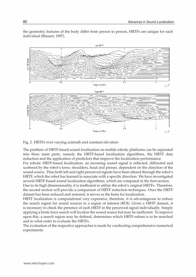
the geometric features of the body differ from person to person, HRTFs are unique for eachindividual (Blauert, 1997).

Fig. 2. HRTFs over varying azimuth and constant elevation

The problem of HRTF-based sound localization on mobile robotic platforms can be separatedinto three main parts, namely the HRTF-based localization algorithms, the HRTF datareduction and the application of predictors that improve the localization performance.For robotic HRTF-based localization, an incoming sound signal is reflected, diffracted andscattered by the robot’s torso, shoulders, head and pinnae, dependent on the direction of thesound source. Thus both left and right perceived signals have been altered through the robot’sHRTF, which the robot has learned to associate with a specific direction. We have investigatedseveral HRTF-based sound localization algorithms, which are compared in the first section.Due to its high dimensionality, it is inefficient to utilize the robot’s original HRTFs. Therefore,the second section will provide a comparison of HRTF reduction techniques. Once the HRTFdataset has been reduced and restored, it serves as the basis for localization.HRTF localization is computational very expensive, therefore, it is advantageous to reducethe search region for sound sources to a region of interest (ROI). Given a HRTF dataset, itis necessary to check the presence of each HRTF in the perceived signal individually. Simplyapplying a brute force search will localize the sound source but may be inefficient. To improveupon this, a search region may be defined, determines which HRTF-subset is to be searchedand in what order to evaluate the HRTFs.The evaluation of the respective approaches is made by conducting comprehensive numericalexperiments.

80 Advances in Sound Localization

www.intechopen.com

2. HRTF Localization Algorithms

In this section, we briefly describe four HRTF-based sound localization algorithms, namelythe Matched Filtering Approach, the Source Cancellation Approach, the Reference SignalApproach and the Cross Convolution Approach. These algorithms return the position of thesound source using the recorded ear signals and a stored HRTF database. As illustrated inFigure 3, the unknown signal S emitted from a source is filtered by the corresponding left andright HRTFs, denoted by HL,i0

and HR,i0, before being captured by a humanoid robot, i.e., the

left and right microphone recordings XL and XR are constructed as

XL = HL,i0· S,

XR = HR,i0· S.

(1)

The key idea of the HRTF-based localization algorithms is to identify a pair of HRTFscorresponding to the emitting position of the source, such that correlation between left andright microphone observations is maximized.

Fig. 3. Single-Source HRTF Model

2.1 Matched Filtering Approach

The Matched Filtering Approach seeks to reverse the HR,i0and HL,i0

-filtering of the unknownsound source S as illustrated in Figure 3. A schematic view of the Matched Filtering Approachis given in Figure 4.

Fig. 4. Schematic view of the Matched Filtering Approach

The localization algorithm is based on the fact that filtering XL and XR with the inverse ofthe correct emitting HRTFs yields identical signals SR,i and SL,i, i.e. the original mono soundsignal S in an ideal case:

81HRTF Sound Localization

www.intechopen.com

SL,i =H−1L,i · XL

=H−1R,i · XR

=SR,i ⇐⇒ i = i0.

(2)

In real case, the sound source can be localized by maximizing the cross-correlation betweenSR,i and SL,i,

arg maxi

{(SR,i

)⊕

(SL,i

)}, (3)

where i is the index of HRTFs in the database and ⊕ denotes a cross-correlation operation.Unfortunately the inversion of HRTFs can be problematic due to instability. This is mainlydue to the linear-phase component of HRTFs responsible for encoding ITDs. Hence astable approximation must be made of the instable version, retaining all direction-dependentinformation. One method is to use outer-inner factorization, converting an unstable inverseinto an anti-causal and bounded inverse (Keyrouz et al., 2006).

2.2 Source Cancellation Algorithm

The Source Cancellation Algorithm is an extension of the Matched Filtering Approach.

Equivalently to cross-correlating all pairs XL · H−1L,i and XR · H−1

R,i , the problem can be restated

as a cross-correlation between all pairs XLXR

andHL,i

HR,i. The improvement is that the ratio of

HRTFs does not need to be inverted and can be precomputed and stored in memory (Keyrouz& Diepold, 2006; Usman et al., 2008).

arg maxi

{(XL

XR

)⊕

(HL,i

HR,i

)}(4)

2.3 Reference Signal Approach

XR= S⋅ H

R ,i0

XL= S⋅ H

L,i0

XR ,out

= S⋅ α

XL,out

= S⋅ β

Fig. 5. Schematic view of the Reference Signal Approach setup

This approach uses four microphones as shown in Figure 5: two for the HRTF-filtered signals(XL and XR) and two outside the ear canal for original sound signals (XL,out and XR,out). Theprevious algorithms used two microphones, each receiving the HRTF-filtered mono soundsignals. The four signals now captured are:

XL = S · HL (5)

XR = S · HR (6)


www.intechopen.com

XL,out = S · α (7)

XR,out = S · β (8)

α and β represent time delay and attenuation elements that occur due to the heads shadowing.

From these signals three ratios are calculated. XLXL,out

and XRXR,out

are the left and right HRTFs

respectively and XLXR

is the ratio between the left and right HRTFs. The three ratios are

then cross correlated with the respective reference HRTFs (HRTF ratios in case of XLXR

). Thecross-correlation coefficients are summed, and the HRTF pair yielding the maximum sum

arg maxi

{(XL

XL,out⊕ HL,i

)+

(XL

XR⊕

HL,i

HR,i

)+

(XR

XR,out⊕ HR,i

)}(9)

defines the incident direction (Keyrouz & Abou Saleh, 2007). The advantage of this systemis that HRTFs can be directly calculated yet retain the original undistorted sound signalsXL,out and XR,out. Thus the direction-dependent filter can alter the incident spectra withoutregard to the contained information, possibly allowing for better localization. However, theneed for four microphones diverges from the concept of binaural localization, exhibiting morehardware and consequently higher costs.

2.4 Convolution Based Approach

To avoid the instability problem, this approach is to exploit the associative propertyof convolution operator (Usman et al., 2008). Figure 6 illustrates the single-sourcecross-convolution localization approach. Namely, left and right observations SR,i and SL,i

are filtered with a pair of contralateral HRTFs. The filtered observations turn to be identical atthe correct source position for the ideal case:

SL,i =HR,i · XL

=HR,i · HL,i0· S

=HL,i · HR,i0· S

=HL,i · XR

=SR,i ⇐⇒ i = i0.

(10)

Similar to the matched filtering approach, the source can be localized in real case by solvingthe following problem:

arg maxi

{(SR,i

)⊕

(SL,i

)}. (11)

2.5 Numerical Comparison

In this section, the previously described localization algorithms are compared by numericalsimulations. We use the CIPIC database (Algazi et al., 2001) for our HRTF-based localizationexperiments. The spatial resolution of the database is 1250 sampling points (Ne = 50 inelevation and Na = 25 in azimut) and the length is 200 samples.In each experiment, generic and real-world test signals are virtually synthesized to the 1250directions of the database, using the corresponding HRTF. The algorithms are then used tolocalized the signals and a localization success rate is computed. Noise robustness of thealgorithm is investigated by different signal-to-noise ratios (SNRs) of the test signals. Itshould be noted that testing of the localization performance is rigorous, meaning, that we


www.intechopen.com

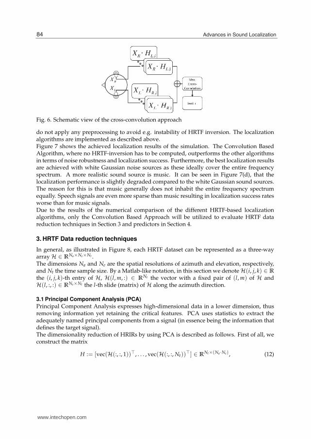
Fig. 6. Schematic view of the cross-convolution approach

do not apply any preprocessing to avoid e.g. instability of HRTF inversion. The localizationalgorithms are implemented as described above.Figure 7 shows the achieved localization results of the simulation. The Convolution BasedAlgorithm, where no HRTF-inversion has to be computed, outperforms the other algorithmsin terms of noise robustness and localization success. Furthermore, the best localization resultsare achieved with white Gaussian noise sources as these ideally cover the entire frequencyspectrum. A more realistic sound source is music. It can be seen in Figure 7(d), that thelocalization performance is slightly degraded compared to the white Gaussian sound sources.The reason for this is that music generally does not inhabit the entire frequency spectrumequally. Speech signals are even more sparse than music resulting in localization success ratesworse than for music signals.Due to the results of the numerical comparison of the different HRTF-based localizationalgorithms, only the Convolution Based Approach will be utilized to evaluate HRTF datareduction techniques in Section 3 and predictors in Section 4.

3. HRTF Data reduction techniques

In general, as illustrated in Figure 8, each HRTF dataset can be represented as a three-wayarray H ∈ R

Na×Ne×Nt .The dimensions Na and Ne are the spatial resolutions of azimuth and elevation, respectively,and Nt the time sample size. By a Matlab-like notation, in this section we denote H(i, j, k) ∈ R

the (i, j, k)-th entry of H, H(l, m, :) ∈ RNt the vector with a fixed pair of (l, m) of H and

H(l, :, :) ∈ RNe×Nt the l-th slide (matrix) of H along the azimuth direction.

3.1 Principal Component Analysis (PCA)

Principal Component Analysis expresses high-dimensional data in a lower dimension, thusremoving information yet retaining the critical features. PCA uses statistics to extract theadequately named principal components from a signal (in essence being the information thatdefines the target signal).The dimensionality reduction of HRIRs by using PCA is described as follows. First of all, weconstruct the matrix

H := [vec(H(:, :, 1))⊤, . . . , vec(H(:, :, Nt))⊤] ∈ R

Nt×(Na ·Ne), (12)


www.intechopen.com

(a) Matched Filtering Approach (b) Source Cancellation Approach

(c) Reference Signal Approach (d) Convolution Based Approach

Fig. 7. Comparison of HRTF-based sound localization algorithms.

where the operator vec(·) puts a matrix into a vector form. Let H = [h1, . . . , hNt]. The mean

value of columns of H is then computed by

μ = 1Nt

Nt

∑i=1

hi. (13)

After centering each row of H, i.e. computing H = [h1, . . . , hNt] ∈ R

Nt×(Na ·Ne) where hi =

hi − μ for i = 1, . . . , Nt, the covariance matrix of H is computed as follows

C := 1Nt

HH⊤. (14)

Fig. 8. HRIR dataset represented as a three-way array


www.intechopen.com

Now we compute the eigenvalue decomposition of C and select q eigenvectors {x1, . . . , xq}

corresponding to the q largest eigenvalues. Then by denoting X = [x1, . . . , xq] ∈ RNt×q, the

HRIR dataset can be reduced by the following

H = X⊤H ∈ Rq×(Na ·Ne). (15)

Note, that the storage space for the reduced HRIR dataset depends on the value of q. Finallyto reconstruct the HRIR dataset one need to compute

Hr = XH + μ ∈ RNt×(Na ·Ne). (16)

We refer to (Jolliffe, 2002) for further discussions on PCA.

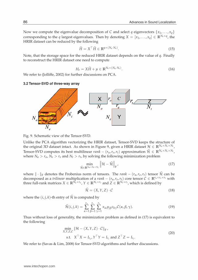
3.2 Tensor-SVD of three-way array

Fig. 9. Schematic view of the Tensor-SVD.

Unlike the PCA algorithm vectorizing the HRIR dataset, Tensor-SVD keeps the structure ofthe original 3D dataset intact. As shown in Figure 9, given a HRIR dataset H ∈ R

Na×Ne×Nt ,

Tensor-SVD computes its best multilinear rank − (ra, re, rt) approximation H ∈ RNa×Ne×Nt ,

where Na > ra, Ne > re and Nt > rt, by solving the following minimization problem

minH∈RNa×Ne×Nt

∥∥∥H− H∥∥∥

F, (17)

where ‖ · ‖F denotes the Frobenius norm of tensors. The rank − (ra, re, rt) tensor H can bedecomposed as a trilinear multiplication of a rank − (ra, re, rt) core tensor C ∈ R

ra×re×rt withthree full-rank matrices X ∈ R

Na×ra , Y ∈ RNe×re and Z ∈ R

Nt×rt , which is defined by

H = (X, Y, Z) · C (18)

where the (i, j, k)-th entry of H is computed by

H(i, j, k) =ra

∑α=1

re

∑β=1

rt

∑γ=1

xiαyjβzkγC(α, β, γ). (19)

Thus without loss of generality, the minimization problem as defined in (17) is equivalent tothe following

minX,Y,Z,C

‖H − (X, Y, Z) · C‖F ,

s.t. X⊤X = Ira , Y⊤Y = Ire and Z⊤Z = Irt .(20)

We refer to (Savas & Lim, 2008) for Tensor-SVD algorithms and further discussions.


www.intechopen.com

3.3 Generalized Low Rank Approximations of Matrices

Fig. 10. Schematic view of the Generalized Low Rank Approximations of Matrices

Similar to Tensor-SVD, GLRAM methods, shown in Figure 10 do not require destruction of a3D tensor. Instead of compressing along all three directions as Tensor-SVD, GLRAM methodswork with two pre-selected directions of a 3D data array.Given a HRIR dataset H ∈ R

Na×Ne×Nt , we assume to compress H in the first two directions.Then the task of GLRAM is to approximate slides (matrices) H(:, :, i), for i = 1, . . . , Nt, of Halong the third direction by a set of low rank matrices {XMiY

⊤} ⊂ RNa×Ne , for i = 1, . . . , Nt,

where the matrices X ∈ RNa×ra and Y ∈ R

Ne×re are of full rank, and the set of matrices {Mi} ⊂R

ra×re with Na > ra and Ne > re. This can be formulated as the following optimizationproblem

minX,Y,{Mi}

Nti=1

Nt

∑i=1

∥∥∥(H(:, :, i)− XMiY⊤)

∥∥∥F

,

s.t. X⊤X = Ira and Y⊤Y = Ire .

(21)

Here, by abuse of notations, ‖ · ‖F denotes the Frobenius norm of matrices. Let us constructa 3D array M ∈ R

ra×re×Nt by assigning M(:, :, i) = Mi for i = 1, . . . , Nt. The minimizationproblem as defined in (21) can be reformulated in a Tensor-SVD style, i.e.

minX,Y,M

‖H − (X, Y, INt) ·M‖F ,

s.t. X⊤X = Ira and Y⊤Y = Ire .(22)

We refer to (Ye, 2005) for more details on GLRAM algorithms.GLRAM methods work on two pre-selected directions out of three. There are then in total three differentcombinations of directions to implement GLRAM on an HRIR dataset. Performance of GLRAM indifferent directions might vary significantly. This issue will be investigated and discussed in section3.5.

3.4 Diffuse Field Equalization (DFE)

A technique that provides good compression performance is diffuse field equalization. Thetechnique reduces the number of samples per HRIR, yet retains the original characteristics.We define the matrix H containing the HRTFs as

H := [vec(H(:, :, 1)), . . . , vec(H(:, :, Nt))] ∈ R(Na ·Ne)×Nt , (23)


www.intechopen.com

where the operator vec(·) puts a matrix into a vector form. Let H = [h1, . . . , h(Na ·Ne)].DFE removes the time delay at the beginning of each HRTF and then calculates the averagepower spectrum from all HRTFs, which then is deconvolved from each HRTF, thus removing

direction-independent information. The average power h is computed by

h = F−1{1

(Na · Ne)

(Na ·Ne)

∑i=1

|F{hi}|2}, (24)

where F{·} denotes the fourier transform. Then, h is shifted circularily by half the kernellength:

h1 = [h(Nt

2+ 1 . . . Nt) h(1 . . .

Nt

2)]. (25)

The filter kernel h1 is inverted and minimum phase reconstruction is applied, yielding h−11 .

The diffused field equalized dataset is retrieved by

hDFE = [(h1 ∗ h−11 ), . . . , (h(Na ·Ne) ∗ h−1

1 )]. (26)

After retrieving the dataset hDFE the time delay samples at the beginning of each HRIR canbe removed. To achieve higher compression of the dataset, also samples at the end of eachHRTFs, which do not contain crucial direction dependent information, can be removed. Forfurther information on DFE see (Moeller, 1992).

3.5 Numerical Comparison

In this section, PCA, GLRAM, Tensor-SVD and Diffused Field Equalization are appliedto a HRTF-based sound localization problem, in order to evaluate performance of thesemethods for data reduction. In each experiment, left and right ear KEMAR HRTF arereduced with one of the introduced reduction methods. A test signal, which is white noiseis virtually synthesized using the corresponding original HRTF. The convolution based soundlocalization algorithm as descirbed in Section 2.4, is fed with the restored databases and usedto localize the signals. Finally, the localization success rate is computed.As already mentioned, GLRAM works on two preselected directions out of three. Therefore,we conduct localization experiments for a subset of directions (35 randomly chosen locations)to detect a combination of well working parameters for GLRAM. After finding a suitablecombination of the variables, localization experiments for all 1250 directions are conducted.Firstly, the dataset is reduced for the first two directions, i.e. elevation and azimuth. Thecontour plot given in Figure 11(a) shows the localization success rate for a fixed pair ofvalues (Nra , Nre ). Similar results with respect to the pairs (Nra , Nrt ) and (Nre , Nrt ) are ploted inFigure 11(b) and Figure 11(c), respectively. Clearly, applying GLRAM on the pair of (Nre , Nrt )outperforms the other two combinations.The application of GLRAM in the directions of elevation and time performs best, therefore,we compare this optimal GLRAM with the standard PCA and Tensor-SVD. As mentioned insection 3.3, GLRAM is a simple form of Tensor-SVD with leaving one direction out. Thus, weinvestigate the effect of additionally reducing the third direction, whereas the dimensions inelevation and time are fixed to the parameters of the optimal GLRAM. Figure 13 shows thatadditionally decreasing the dimension in azimuth leads to a huge loss of localization accuracy.After determining the optimal parameters for GLRAM, the simulations are conducted forall 1250 directions of the CIPIC dataset. Figure 12 shows the localization success rate independency of the compression rate for GLRAM and PCA. It can be seen that an optimizedGLRAM outperforms the standard PCA in terms of compression.


www.intechopen.com

(a) GLRAM on (azimuth, elevation) (b) GLRAM on (azimuth, time)

(c) GLRAM on (elevation, time)

Fig. 11. Contour plots of localization success rate of using GLRAM in different settings.

Fig. 12. Comparison between DFE, PCA and GLRAM

4. Predictors for HRTF sound localization

To reduce the computational costs of HRTF-based sound localization, especially for movingsound sources, it is advantageous to determine a region of interest (ROI) as illustrated inFigure 15. A ROI constricts the 3D search space around the robotic platform leading to areduced set of eligible HRTFs.Various tracking models have been implemented in microphone sound localization. Primarilythey predict the path of a sound source as it is traveling and thus acquiring faster and moreaccurate non-ambiguous localization results (Belcher et al., 2003; Ward et al., 2003). Most ofthese filters are updated periodically in scans. In this section, three predictors, namely Time


www.intechopen.com

Delay of Arrival, Kalman filter and Particle filter, are briefly introduced to determine a ROI toreduce the set of eligible HRTFs to be processed to localize moving sound sources.

4.1 Time Delay of Arrival

The time delay between the two signals xi[n] and xj[n] is found when the cross-correlationvalue Rij(τ) is maximal. Given that τ has been determined, the time delay is calculated by

∆T =τ

fs, (27)

where fs is the sampling rate. Knowing the geometry (distance between the robot’s ears) of themicrophones and the delays between microphone pairs, a number of locations for the soundsource can be disregarded (Brandstein & Ward, 2001; Kwok et al., 2005; Potamitis et al., 2004;Valin et al., 2003). Then, an HRTF-based localization algorithm only evaluates the remainingpossible locations of the source.

4.2 Kalman Filter

The Kalman filter is a frequently used predictor (usage for microphone array localizationdescribed in (Belcher et al., 2003)). The discrete version exhibits two main states: time update(prediction) and measurement update (correction). The Kalman filter predicts the state of xk

at time k given the linear stochastic difference equation

xk = Axk−1 + Buk−1 + wk−1 (28)

and measurementzk = Hxk + vk. (29)

Matrices A, B and H provide relation from discrete time k− 1 to k for their respective variablesx (the state) and u (optional control input). w and v add noise to the model. A set of time andmeasurement update equations are used to predict the next state (Kalman, 1960). The statevector is defined by current location coordinates x and y and the velocity components vx andvy (Potamitis et al., 2004; Usman et al., 2008). Note that here the predictor is applied to twodimensional space.

x = [x, vx, y, vy]T (30)

An unreliable location estimate during initialization of the the Kalman filter may be a sourceof error. To improve upon this, particle filters have been implemented in (Chen & Rui, 2004).

Fig. 13. Localization success rate by Tensor-SVD


www.intechopen.com

"%&! #1)'/.:'610

#1)'610 $3+*.)610

%+*8)+* 4+5 1, 0+95 2144.(/+

/1)'6104 51 4+'3)-

actual

position update

position

prediction

Fig. 14. Schematic view of the application of predictors in HRTF-based localization.

4.3 Particle Filter

The particle filter bases itself on the idea of randomly generating samples from a distributionand assigning weights to each to define their reliability. The particles and their associatedweights define an averaged center which is the predicted value for the next step. Each weightwi

k is associated to a particle xi in iteration k. A set of N particles is initially drawn from

a distribution q(xi|xik−1, zk) with zk being the current observed value. For each particle the

weight is calculated by

wik = wi

k−1

p(zk|xik)p(xi

k|xik−1)

q(xik|x

i0:k−1, z1:k)

. (31)

Once all weights are calculated, their sum is normalized. To determine the predicted value,the weighted average of the particles is taken:

x =1

N

N

∑i=1

wik · xi (32)

Over time it may occur that very few particles possess most of the weight. This case requiresresampling to protect from particle degeneration. The variance of the weights is used as ameasure to check for this case and if required, the set of weights is exchanged with a betterapproximation (Gordon et al., 1993).Many particle filter variations exist, such as the Monte Carlo approximations and SamplingImportance Resampling. However a particle filter may find only a local optimum and thusnever reaching the global optimum. Evolutionary estimation is proposed in (Kwok et al.,2005) to overcome such problems. Initially a set of potential speaker locations are estimatedand then a heuristic search is performed. The speaker locations are called chromosomes andcan only move within a defined region. After the initialization, the Time Delay of Arrival(TDOA) is evaluated for each potential location as well as each microphone. The difference vi

between expected and actual TDOAs is used to define a fitness function for each chromosomei together with error variance σ2

τ :

ωi = e−0.5

v2i

σ2τ (33)

ωi is then scaled such that ∑ni=1 ωi = 1 → ωi The new estimate of source location is given by

sx =n

∑i=1

ωisxi. (34)


www.intechopen.com

(a) Time Delay of Arrival

(b) Particle Filter

(c) Kalman Filter

Fig. 15. Comparison of predictors for HRTF Sound Localization.


www.intechopen.com

Chromosomes are then selected according to a linearly spaced pointer spanning the fitnessmagnitude scale, with higher fitness chromosomes being selected more often. The latterchromosomes receive less mutation as compared to weaker chromosomes depending on rg,the zero mean Gaussian random number variance, and dm, the distance for mutation (Kwoket al., 2005).

sxi+1 = sxi + rgdm (35)

4.4 Numerical comparison

This section gives a performance overview of the applied predictors in a HRTF-based soundlocalization scenario. We simulate moving sound by virtually synthesizing a sound source,which is white noise, using different pairs of HRTFs. This way, a random path of 500 differentsource positions is generated, simulating a moving sound source. Then, Time Delay of Arrival,the Kalman filter and the Particle filter seek to reduce the search region for the HRTF-basedsound localization to a region of interest. The Convolution Based Algorithm is utilized tolocalize the moving sound source. The experiments were conducted three times with differentspeed of the sound source.Figure 15 summarizes the results of applying predictors to HRTF-based sound localization.The left plots show the localization success rates in dependency of the size of the region ofinterest. In the right plots the number of directions that have to be evaluated within thelocalization algorithms are shown. The bigger the region of interest, the more HRTF-pairshave to be utilized to maximize the cross correlation (11) resulting in a higher processing time.On the other hand, the smaller the region of interest, the higher the danger of excluding theHRTF pair that is maximizing the cross correlation (11), leading to false localization results.Our simulation results show that the number of HRTFs to be evaluated for the ConvolutionBased Algorithm can be significantly reduced to speed up HRTF-based localization formoving sources. Time Delay of Arrival is reducing the search region to 500 directions whilereaching hundred percent correct localization of the path, meaning all 500 source positions aredetected correctly for the different speeds of the sources. Particle- and Kalman filter are ableto reduce the search region to 130 directions in case of sound sources with a speed of 20deg/s.For slower sources, only 60 directions need to be taken into account.

Acknowledgements

This work was fully supported by the German Research Foundation (DFG) within thecollaborative research center SFB-453 "High Fidelity Telepresence and Teleaction".

5. References

Algazi, V. R., Duda, R. O., Thompson, D. M. & Avendano, C. (2001). The CIPIC HRTFdatabase, IEEE ASSP Workshop on Applications of Signal Processing to Audio andAcoustics, New Paltz, NY, pp. 21–24.

Belcher, D., Grimm, M. & Kroschel, K. (2003). Speaker tracking with a microphone array usinga kalman filter, Advances in Radio Science 1: 113–117.

Blauert, J. (1997). An introduction to binaural technology, Binaural and Spatial Hearing, R.Gilkey, T. Anderson, Eds., Lawrence Erlbaum, Hilldale, NJ, USA, pp. 593–609.

Brandstein, M. & Ward, D. (2001). Microphone arrays - signal processing techniques andapplications, Springer.


www.intechopen.com

Chen, Y. & Rui, Y. (2004). Real-time speaker tracking using particle filter sensor fusion,Proceedings of the IEEE 92(3): 485–494.

Gordon, N., Salmond, D. & Smith, A. (1993). Novel approach to nonlinear/non-GaussianBayesian state estimation, Radar and Signal Processing, IEE Proceedings F 140(2): 107–113.

Jolliffe, I. T. (2002). Principal Component Analysis, second edn, Springer.Kalman, R. (1960). A new approach to linear filtering and prediction problems, Transactions of

the ASME - Journal of Basic Engineering 82(Series D): 35–45.Keyrouz, F. & Abou Saleh, A. (2007). Intelligent sound source localization based on

head-related transfer functions, IEEE International Conference on Intelligent ComputerCommunication and Processing, pp. 97–104.

Keyrouz, F. & Diepold, K. (2006). An enhanced binaural 3D sound localization algorithm,2006 IEEE International Symposium on Signal Processing and Information Technology,pp. 662–665.

Keyrouz, F., Diepold, K. & Dewilde, P. (2006). Robust 3D Robotic Sound Localization UsingState-Space HRTF Inversion, IEEE International Conference on Robotics and Biomimetics,2006. ROBIO’06, pp. 245–250.

Kwok, N., Buchholz, J., Fang, G. & Gal, J. (2005). Sound source localization: microphonearray design and evolutionary estimation, IEEE International Conference on IndustrialTechnology, pp. 281–286.

Moeller, H. (1992). Fundamentals of binaural technology, Applied Acoustics 36(3-4): 171–218.Potamitis, I., Chen, H. & Tremoulis, G. (2004). Tracking of multiple moving speakers

with multiple microphone arrays, IEEE Transactions on Speech and Audio Processing12(5): 520–529.

Savas, B. & Lim, L. (2008). Best multilinear rank approximation of tensors with quasi-Newtonmethods on Grassmannians, Technical Report LITH-MAT-R-2008-01-SE, Departmentof Mathematics, Linkpings University.

Usman, M., Keyrouz, F. & Diepold, K. (2008). Real time humanoid sound source localizationand tracking in a highly reverberant environment, Proceedings of 9th InternationalConference on Signal Processing, Beijing, China, pp. 2661–2664.

Valin, J., Michaud, F., Rouat, J. & Letourneau, D. (2003). Robust sound source localizationusing a microphone array on a mobile robot, IEEE/RSJ International Conference onIntelligent Robots and Systems, Vol. 2.

Ward, D. B., Lehmann, E. A. & Williamson, R. C. (2003). Particle filtering algorithms fortracking an acoustic source in a reverberant environment, IEEE Transactions on Speechand Audio Processing 11(6): 826–836.

Ye, J. (2005). Generalized low rank approximations of matrices, Machine Learning61(1-3): 167–191.


www.intechopen.com

Advances in Sound LocalizationEdited by Dr. Pawel Strumillo

ISBN 978-953-307-224-1Hard cover, 590 pagesPublisher InTechPublished online 11, April, 2011Published in print edition April, 2011

InTech EuropeUniversity Campus STeP Ri Slavka Krautzeka 83/A 51000 Rijeka, Croatia Phone: +385 (51) 770 447 Fax: +385 (51) 686 166www.intechopen.com

InTech ChinaUnit 405, Office Block, Hotel Equatorial Shanghai No.65, Yan An Road (West), Shanghai, 200040, China

Phone: +86-21-62489820 Fax: +86-21-62489821

Sound source localization is an important research field that has attracted researchers' efforts from manytechnical and biomedical sciences. Sound source localization (SSL) is defined as the determination of thedirection from a receiver, but also includes the distance from it. Because of the wave nature of soundpropagation, phenomena such as refraction, diffraction, diffusion, reflection, reverberation and interferenceoccur. The wide spectrum of sound frequencies that range from infrasounds through acoustic sounds toultrasounds, also introduces difficulties, as different spectrum components have different penetrationproperties through the medium. Consequently, SSL is a complex computation problem and development ofrobust sound localization techniques calls for different approaches, including multisensor schemes, null-steering beamforming and time-difference arrival techniques. The book offers a rich source of valuablematerial on advances on SSL techniques and their applications that should appeal to researches representingdiverse engineering and scientific disciplines.

How to referenceIn order to correctly reference this scholarly work, feel free to copy and paste the following:

Martin Rothbucher, David Kronmüller, Marko Durkovic, Tim Habigt and Klaus Diepold (2011). HRTF SoundLocalization, Advances in Sound Localization, Dr. Pawel Strumillo (Ed.), ISBN: 978-953-307-224-1, InTech,Available from: http://www.intechopen.com/books/advances-in-sound-localization/hrtf-sound-localization

© 2011 The Author(s). Licensee IntechOpen. This chapter is distributedunder the terms of the Creative Commons Attribution-NonCommercial-ShareAlike-3.0 License, which permits use, distribution and reproduction fornon-commercial purposes, provided the original is properly cited andderivative works building on this content are distributed under the samelicense.

https://creativecommons.org/licenses/by-nc-sa/3.0/

hrtf sound localization - intech - open science open minds

Documents