https www.safety.duke.edu radsafety drdl modules rp 12 rp
TRANSCRIPT
The United States Nuclear Regulatory Commission and Duke University
Present: Regulatory and Radiation Protection Issues in Radionuclide Therapy
Copyright 2008 Duke Radiation Safety and Duke University. All Rights Reserved.

Welcome!
This is the Eleventh of a series of training
modules in Radiation Physics.
These modules provide a basic introduction
to h matter.
Sponsored by the United States Nuclear
Regulatory Commission and Duke University
Author: Dr. Rathnayaka Gunasingha, PhD

Your Instructor
Dr. Rathnayaka Gunasingha is an
Accelerator Physicist with
background in High Energy physics.
Dr. Gunasingha is a physicist in the
Radiation Safety division and
member of the Faculty of the Duke
Medical Physics Graduate Program.
Contact:

Goals of the Course
Upon completing these instructional
modules, you should be able to:
understand the Basic Interaction of Radiation with
Matter
apply the knowledge in various calculations used
in Medical and Health Physics
understand the basic principles behind various
instrumentation used in Medical and Health
Physics

This Module Will Cover
The General properties of Detectors such as,
1. Modes of operation
2. Methods of recording data
3. Energy resolution
4. Efficiency of detectors
5. Dead time and dead time measurements
General properties of Detectors
• There are two types of detectors
1. Active detectors
2. Passive detectors.

General properties of Detectors
1. Active detectors:
provide immediate results (“signal”), usually by
means of electric current or current pulses
2. Passive detectors:
Radiation effects of these detectors are read
after eradiation. Signal consist of changes of
diverse nature – electrical, mechanical, optical,
chemical.

General properties of Detectors
• Simple detector model:
Radiation undergo some interactions and deposit the
energy. Net result is the appearance of charge Q
created by ionization within the detector volume and
producing a
General properties of Detectors
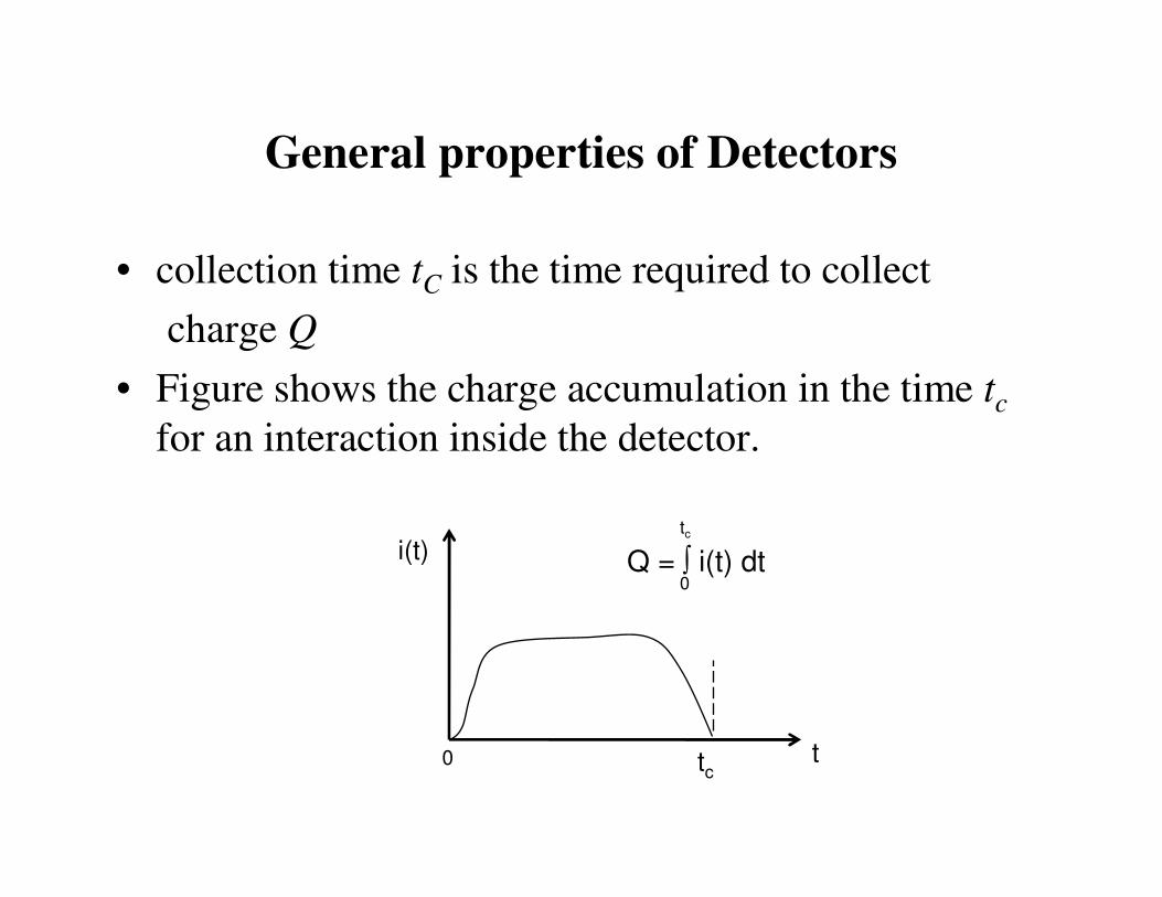
• collection time tC is the time required to collect
charge Q
• Figure shows the charge accumulation in the time tc
for an interaction inside the detector.
i(t)
tct0
Q = ∫ i(t) dt
tc
0

General properties of Detectors
• A pulse is due to one interaction.
• Assume the rate of irradiation is low so that we can
identify individual pulses as shown in figure.
• The size and duration of each current pulse depends
on type of interaction.
t
i(t)

Modes of operations
There are three modes of detector operations:
(1) Current mode
(2) Pulse mode
(3) Mean square voltage (MSV ) mode
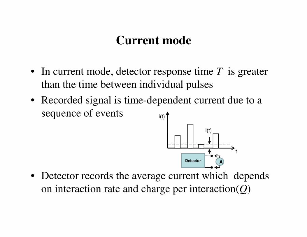
Current mode
• In current mode, detector response time T is greater
than the time between individual pulses
• Recorded signal is time-dependent current due to a
sequence of events
• Detector records the average current which depends
on interaction rate and charge per interaction(Q)
t
i(t)
I(t)
Detector A
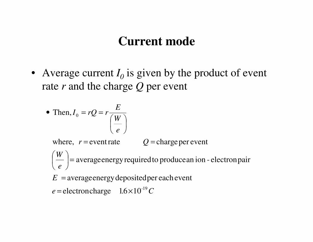
Current mode
• Average current I0 is given by the product of event
rate r and the charge Q per event
C.e
E
e
W
Qr
e
W
ErrQI
-19
0
1061 chargeelectron
eventeach per depositedenergy average
pairelectron -ionan produce torequiredenergy average
eventper charge rateevent where,
Then,
×=
=
=
==
==•

General properties of Detectors
Figure shows the
fluctuations of current with
time
σ σ σ
σ
+
′= − ⇒ =
•
=
∫
I(t) = fluctuating current
Standard deviation for recorder events are
given by
If each pulse contribute the same charge
functional standard deviati
2t T2 2
I 0 I I
t
n
1(t ) I(t ') I dt (t) (t)
T
rT
σ σ= =
on of the measured
signal is
I n
0
(t) 1
I n rT
I0
I(t)
t
σi(t)

Mean Square Voltage Mode(MSV)
( )
( )
This mode is called the "Campbell mode"
Since
This mode is useful to measure mixed fields
(neutron vs. gamma fields).
Circuit measures the current fluctuations
and computes the
2 2
i
i
t Q
t
σ
σ
•
• ∝
•
square of their time average

Pulse mode
• Current mode is good when event rates are very high.
• MSV mode is good for large amplitude events
• Event rate or time information is needed pulse mode
is used.
Pulse mode
• In this mode, detector records the charge from
individual event interaction
• Usually more desirable for getting information on
amplitude and timing of individual pulses
• Not suitable for very high event rates – time between
adjacent events are too short for analysis
• Energy deposited ~ Q – enables particle spectroscopy

Pulse mode
• Output from an event depends on the counting circuit
( detector + preamplifier)
• R = input resistance of circuit
• C = equivalent capacitance of detector system
• Signal voltage V(t) depends on time constant
τ = RC
V(t)=V0(1-e-t/RC)Detector = V(t)C R
preamplifier

Pulse mode
Figure shows current output and voltage output for two cases.
tC= charge collection time
1. When RC<< tC
Current through R is instantaneous value in the detector.
Equivalent signal is shown in figure (b)
V(t) = Ri(t)
it can collect charge for a single
event with tc.
i(t)
tc
t0
Q = ∫ i(t) dt
tc
0

Pulse mode
If time between pulses are longer,
capacitor discharge through R
Output voltage V(t) is shown in
figure ( c ).
When RC >> tC
Very little current flows through R
during tC.
Detector current is integrated on
capacitor
V(t)
0t
RC << tcV(t) = Ri(t)
V(t)
t0
RC >> tcVmax = Q/C
Vmax

Pulse mode
• This is the most common means of pulse type operation.
The reasons are
1. tC determines the time required for a signal to reach to maximum ( it does not depend on the external circuit)
2. Since Vmax = Q/C
The amplitude of the output pulse is directly proportional to the energy of the radiation

Pulse mode
Advantages in pulse mode:
1. Sensitivity is greater than when using current or MSV mode.
2. Lower limit is set by the background radiation
3. Pulse amplitude carries some information on charge generated by event
- in other modes ( current or MSV) this information is lost.
- all interactions contribute to the average value of the output current
Pulse Height Spectra
• When detector is operated in pulse mode, the pulse amplitudes carry information regarding charges generated
• Amplitudes of the pulses are not the same, due to the differences in radiation energy or fluctuations of the detector
• We get a differential pulse height distribution dN/dH
• dN is the number of counts in dH energy bin
• This can be obtained using a multi-channel analyzer (MCA)

Pulse Height Spectra
Common way to display pulses is through a
differential pulse height distribution
The number of pulses between and
is given by 2
1
1 2
H
0
H
H H
dNdH N
dH
•
•
=∫
0H (volt)
Differential pulse height spectrumdN/dH
(volt)-
1
H1 H2
maximum H
Pulse height (H)

Pulse Height Spectra
• Another method of displaying pulse height is
Integrated pulse height distribution
X axis ( abscissa) is the same
pulse height as before.
Ordiante ( y axis ) represents
the number of pulses whose
amplitude exceeds that of a
given value of H.
At the origin, the value of y, is
N0
0H (volt)
N0
num
ber
of
puls
es
N
exceedin
g H
H3 H4
plateau

Energy Resolution
• Spectroscopy: response to mono-energetic sources
such as gamma ray or alpha particles
• Pulse height distribution from a detector is called
“response function”
•If all the pulses are
around H0, good
resolution means
little fluctuation in
pulse height. 0H (volt)
dN/dH
(volt)-
1
H0
good resolution
pulse height (H)
poor resolution

Energy Resolution
• Energy Resolution of a detector is defined as
Rule of thumb is,
one can separate two
energies H2, H1, if
H2 – H1 > FWHM
Smaller the value of R, the
better the detector will be able
to resolve energies lying
closer
Where =Full width at Half Maximum
0
FWHMR
H
FWHM
=
0H (volt)
dN/dH
H0
R = FWHM / H0h
h/2 FWHM
σ

Energy Resolution
• There are number of Sources of fluctuations:
a) Drift of detector operating characteristics ( HV,
gain ..)
b) random noise in detector & electronics
c) statistical noise intrinsic to nature of signal
(discrete number of charge carriers, fluctuations
in energy deposition in detector)
• C) will dominate because it is always in a detector
system
Energy Resolution
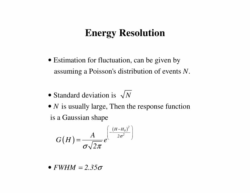
( )
Estimation for fluctuation, can be given by
assuming a Poisson's distribution of events
Standard deviation is
is usually large, Then the response function
is a Gaussian shape
N.
N
N
AG H e
2σ π
•
•
•
=
( )
2
0
2
H H
2
FWHM 2.35
σ
σ
− −
• =

Energy Resolution
Average pulse where constant
standard deviation = and
Energy resolution
0
Posisson Limit
0
H KN K
K N
FWHM 2.35K N
FWHMR
H
2.35K N 2.35R
KN N
σ
• = =
=
=
= =
Energy Resolution
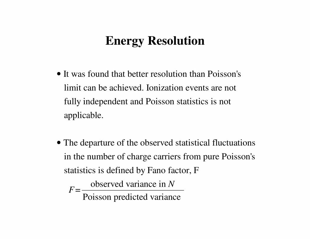
It was found that better resolution than Poisson's
limit can be achieved. Ionization events are not
fully independent and Poisson statistics is not
applicable.
The departure of the observed s
•
• tatistical fluctuations
in the number of charge carriers from pure Poisson's
statistics is defined by Fano factor, F
observed variance in =
Poisson predicted variance
NF

Energy Resolution
Because variance is the equivalent equation
for semiconductor detectors and propotional
counters, for scintillators
Adding all sources of fluctuations ( Ga
2
limit
,
2.35K N F FR 2.35
KN N
F 1
F 1
σ•
= =
• <
≈
•
( ) ( ) ( ) ( )
uss)
2 2 2 2
Total stat noise driftFWHM FWHM FWHM FWHM .....= + +

Detection Efficiency
• Charged particles or ions immediately interact within
the detector volume as soon as they enter the detector
Every pulse can be recorded and detector is almost
100% efficient.
• Gamma and neutron travel a large distance before
they interact within the detector. Therefore, the
efficiency for uncharged particles is less than 100%

Detection Efficiency
There are two classes of efficiency
1. Absolute efficiency
2. Intrinsic efficiency
Absolute efficiency is defined as
number of particles recorded
number of part
abs
int
det ected
abs
( N )
η
η
η
•
•
=icles emitted by source(
depends on the detector properties and geometry
emitted
abs
N )
η•

Detection Efficiency
Intrinsic efficiency is defined as
number of pulses recorded( )
number of radiation incident on detector( )
depends on detector properties only
Taking ratio of and
det
int
inci
int
abs int
N
N
,
η
η
η η
•
=
•
•
abs inci
int emitted
N
N
η
η=

Detection Efficiency
From the diagram,
inci
emitted
abs int
N
N 4
4
π
η ηπ
•
Ω=
Ω • =
• Usually not all the pulses are of interest. For instance, in
spectroscopy, only the pulses around peak are desired.
Peak efficiency εpeak is determined considering
pulses around the peak.
Ω
a
Ω = A/l2 = πa2/l2
A
l
πa2/4πl2 = Ω/4π
S

Detection Efficiency
is calculated counting all interactions.
peak-to-total ratio is defined by
Figure shows peak area and total area.
total
peak
total
r
ε
ε
ε
•
•
=
•
Intrinsic peak efficiency
most commonly tabulated
for gamma detectors
0H (volt)
dN/dH
Full energy peak
Dead Time
• A detector that responds sequentially for individual
events, requires a minimum amount of time that
should separate two events in order that events be
recorded as two separate events.
• This minimum time is called the “Dead Time”
• Dead time may be due to:
a. processes in the detector
b. counting electronics

Dead Time
• In a random sample, two events may occur very close in time, and some true events may be lost due to the dead time
• There are two methods to determine the true number of events
1. paralyzable detector method
2. nonparalyzable detector method
• Dead time τ is set after each true event that occurred during the “live period”

Dead Time
• Paralyzable detector method:
Any event occurred during dead period not recorded as
counts, but it extends the dead period t following the lost
event.
• Non paralyzable detector method:
it just ignore the other event occurred during dead period
t
Following example shows the difference between
paralyzable and nonparalyzable events

Dead Time
The middle line represents 10 events along the time axis as they come.
Assume events 3,4 and 6,7,8 come very close in time (i.e. within the
dead time of previous event)
Five events in
paralyzable method
Seven events in
nonparalyzable method
1 3 4 75 6 8 92 10
events in the detectorTime
nonparalyzable
paralyzableτ
Dead
Live
Dead
Live

Dead Time
Events 1,9 and 10 are recorded by both detectors.
After event 2 is registered, event 3 and 4 restart the dead
period for paralyzable detector which misses both event 3
and 4.
In non paralyzable method, after event 2 is registered, it
recovers to register event 4. ( event 3 is lost since it is
within dead time of event 2 and event 4 is outside the
dead time of 2)

Dead Time
• After event 5 is recorded, paralyzable detector extends the
dead period from events 6,7, and 8. As a result, all events
6,7,8 are lost.
• In non-paralyzable detector, after event 5 is recorded, it
recovers to record the event 7. Only event 6 and 8 are lost
as they are within dead time of event 5 and 7 respectively.

Nonparalyzable Detector Method
Let us obtain an expression for true interaction
rate. Dead time is a fixed value for each event
in this method.
assume n= rate of true interactions
m= rate of measured events
•
= dead time for one event
Then,
fraction of time detector is dead = m
fraction of time detector is sensitive = 1-m
τ
τ
τ

Nonparalyzable Detector Method
Fraction of true events recorded =
Using , appropriate correction can be made to
measured data .
m
n
m1 m
n
mn
1 m
n
m
τ
τ
•
= −
=−
•

Paralyzable Detector Method
• The dead τ is not fixed in this method. As you saw in the example, dead time depends on how close the events are.
• In this method, only intervals longer than τ are registered. We need to find the distribution of time intervals between consecutive random events.
Paralyzable Detector Method
Let us assume, true events rates to be
Then, the average number of events occur in time
if first event occur at
probability that no event occur in time , after
first event(Poisson ter
n
t nt
t 0,
t
•
=
=
m)
Probability that an event occurs in next time
interval
nt
0P e
dt ndt
−=
=

Paralyzable Detector Method
After first event at ,
The probability that the next event occur
between and
Where = probability of observing an interval
whose length lies between
nt
t 0
t t dt p( t )dt ne dt
p( t )dt
dt
−
=
+ → =
about
The probability of intervals larger than
nt n
t
p( ) p( t )dt ne dt e τ
τ τ
τ
τ∞ ∞
− −= = =∫ ∫

Paralyzable Detector Method
Then, observed count rate is
For low event rate or slow dead time
Here, the true rate , can not be solved explicitly.
If and are known,
n
m
m ne
( n 1)
m n(1- n )
n
m
τ
τ
τ
τ
−=
<<
=
can be solved iteratively.n

Paralyzable Detector Method
Figure shows the plot of measured count rate m, as a
function of true rate n for both models
m
n1/τ
1/τ
0
1/eτ
paralyzable
nonparalyzable
m =
n
Paralyzable Detector Method
• In non-paralyzable model m can not exceed the value
. When n increases m approaches an asymptotic value.
• For paralyzable model, (using calculus) m has a maximum value (1/eτ) at n=1/τ. After that m decreases to zero with increasing n.
• Also, in this model, there could be two possible event rates n, for one measured rate m.
1
τ

Dead Time
( )
( )
Low rates or slow dead time i.e.
For non paralyzable model
For paralyzable model
So, both model agree in the limit of low rate or
slow dead time
n
n n 1
nm n 1 n
1 n
m ne n 1 n
n
τ
τ
ττ
τ
τ
−
•
= = −+
= = −

Dead Time Measurements
In order to make dead time correction for
observed events, we should know
There are two methods to measure
1. two source method
2. decay source method
m τ
τ
•
•

Dead Time Measurements
two source method
In this method, counting rate is observed individually
and in combination.
Assume,
and be true counting rates for sources 1, 2 and
combined
and
1 2 12
1 2
n ,n n
m ,m
•
m be observed counting rates for
sources 1, 2 and combined
n and m are the background rates for true and
observed
12
b b

Dead Time Measurements
( ) ( ) Then,
Using non-paralizable model value for each
12 b 1 2 bb
12 b 1 2
b12 1 2
12 b 1 2
n n n n n n
n n n n
n
mm m m
1 m 1 m 1 m 1 mτ τ τ τ
• − = − + −
+ = +
+ = +− − − −

Dead Time Measurements
( )( )
Solve for ,
=1 2 1 2 12 1 12 2
1 2 12
m m m m m m m m
m m m
τ
τ
•
− − −

Dead Time Measurements
Decay method:
A short lived source is used.
Assume is the true rate at and is the decay
constant
Assume, background is very small
Assume non-paralyzable method
0
b
t
0
n t 0
n n
n n eλ
λ
−
•
=
=
t
0 0
mn
1 m
me n m nλ
τ
τ
=−
= − +
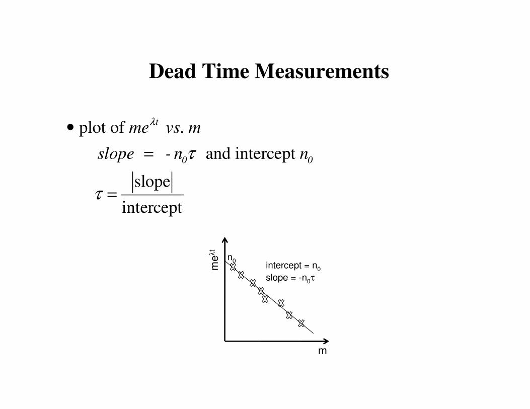
Dead Time Measurements
plot of
and intercept
slope
intercept
t
0 0
me vs. m
slope - n n
λ
τ
τ
•
=
=
intercept = n0
slope = -n0τ
n0
me
λt
m
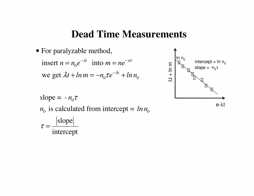
Dead Time Measurements
For paralyzable method,
insert into
we get
slope =
is calculated from intercept =
slope
intercept
t n
0
t
0 0
0
0 0
n n e m ne
t ln m n e ln n
- n
n ln n
λ τ
λλ τ
τ
τ
− −
−
•
= =
+ = − +
=
intercept = ln n0
slope = -n0τ
ln n0
λt
+ ln
m
e-λt

Dead Time Losses
• In all of the previous methods, we assumed radiation
from steady state sources. For these sources,
probability of an event occurring per unit time is a
constant (Poisson’s statistics)
• Some events are lost due to dead time and distribution
intervals are modified and it may deviate from
Poisson’s behavior.

Dead Time Losses from non-continuous
sources
• Radiation sources such as electron accelerators used
to generate X-rays are operated in pulse mode
• As shown in figure, it can have pulse duration T with
few microseconds and repetition frequency f with few
kW.
1/f
T

Dead Time Losses from Pulsed Source
If , source is pulsed has little effect
steady state source results can be applied
If only a small number counts may be
recorded by the detector. This is more
complicated and not cons
T
T
τ
τ
•
• ≤
ider here
If and only one count
per source pulse and detector will be recovered
before next pulse.
1T T ,
fτ τ
• < −
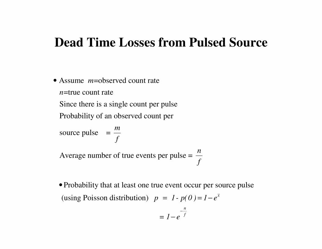
Dead Time Losses from Pulsed Source
Assume =observed count rate
=true count rate
Since there is a single count per pulse
Probability of an observed count per
source pulse =
Average number of true events per pulse =
m
n
m
f
•
Probability that at least one true event occur per source pulse
(using Poisson distribution)
=
x
n
f
n
f
p 1- p(0 ) 1 e
1 e−
•
= = −
−

Dead Time Losses from Pulsed Source
Then,
A plot of vs is shown in
figure
when
maximum observable count rate is
n
f
n
f
m1 e
f
m f 1 e
m n
n , m f
f
−
−
• = −
= −
•
• → ∞ →n
m
f
0
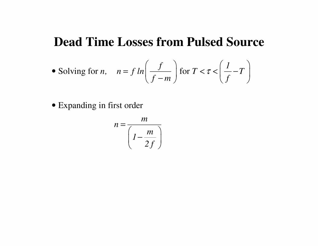
Dead Time Losses from Pulsed Source
Solving for for
Expanding in first order
f 1n, n f ln T T
f m f
mn
m1
2 f
τ
• = < < − −
•
=
−
Credits and References
Tsoulfanidis. N, Measurement and Detection
of Radiation, McGraw-Hill, New York(1983)
G.F.Knoll, Radiation Detection and
Measurement, 3rd ed. , John Wiley & Sons