http___=miamiimageurl&_cid=271461&_user=512776&_pii=0043164885901759&_check=y&_coverdate=1985-04-15&view=c&wchp=dglbvlv-zskzs&md5=c996cc84276776aae11b6fa5781ad559_1-s2.0-0043164885901759-main...

8/3/2019 http___www.sciencedirect.com_science__ob=MiamiImageURL&_cid=271461&_user=512776&_pii=00431648859017…

http://slidepdf.com/reader/full/httpwwwsciencedirectcomscienceobmiamiimageurlcid271461user512776pii0043164885901759c… 1/22

Wear, 102 (1985) 309 - 330 309

THE ~FLUENCE OF TURBULENCE ON EROSION BY A

PARTICLE-LIEN FLUID JET

SUDIP DOSANJ H and J OSEPH A. C. HUMPHREY

~ateriu~s and Mo~ec~~r Research Division, Lawrence Berkeley Laboratory, University of

California, Berkeley, CA 94720 (U.S.A.)

(Received J uly 2,1984; accepted Febr ua ry ‘7, 1985)

Summary

Very few investigations on wear by particle impact have accounted forthe influence of turbulence on erosion. In this study, the effects of turbulentdiffusion on particle dispersion, and hence on erosion, are demonstratednumerically. Variations imposed on the level of turbulence intensity in aparticle-laden jet impinging normally on a flat wall show a strong depen-dence of wear parameters on this quantity. Impacting particle velocities,trajectories and surface densities are predicted from lagrangian equationsof motion. Eulerian equations are used to describe fluid motion, with theturbulence viscosity evaluated from a k-e model of turbulence. Nonessential

complexities are avoided by assuming one-way coupling between phases andusing an adjusted Stokes’ drag relation. Numerics calculations reveal thatthe relative rate of erosion decreases and that the location of maximum wearis displaced toward the stagnation point as the turbulence intensity increases,Efforts to remove present model limitations have been hindered by theunav~lability of suitable experiment data,

1.1. Theprablem of interestWhile it has been known for some time that mean flow conditions can

si~ifi~~tly affect erosive wear by particle imp~gement, the rule played byturbulent fluctuations, especially near walls, is neither appreciated norunderstood. As a result there is a significant risk when interpreting erosivewear results of incorrectly accounting for behavioral aspects of the wearprocess that are associated with the turbulent nature of the flow. In an earlystudy by Finnie 111, it was suggested that surface erosion by particle impactshould increase with increased turbulence levels in some flows. However, todate the phenomenon has not been investigated systematically and in depth.As a result there does not exist a satisfactory database for guiding fundamen-tal theoretical interpretation and the development of predictive modelswhich account for the influence of turbulence on erosive wear.

@ Elsevier Sequoial~inted in Switzerta nd



310

In free shear flows it has been established that turbulent fluctuations

affect particle dispersion. Some of the experimental data available for the

particle-laden jet configuration have been reviewed and extended by Faeth

[2 J and Shuen et al. [3] and discussed by Melville and Bray [4] and Crowderet caE. [ 5 J. Following Pourahmadi and Humphrey [ 6 J, the latter workers

modeled particle dispersion in a turbulent mixing layer flow using eulerian

forms of the transport equations and allowing two-way coupling between

the continuous fluid and the solid phases.

As illustrated by, for example, Melville and Bray [73 and Po~~madi

and Humphrey [ 61, the in~ract~g continua approach facilitates the formu-

lation of two-phase flow turbulence modeling concepts, However, it does not

yield unambiguous specifications of impact velocity and impact angle on

collision of a particle with a surface. A knowledge of these two parameters is

essential for any useful model of erosive wear. For this reason, it was decided

to investigate the influence of turbulence on particle motion, and hence on

erosion, using a lagrangian description for the motion of the solid phase. To

simplify matters initially, particle motion was attributed entirely to the

mean flow (drag) differences between phases. As a result, turbulence-

enhanced diffusion of the particle phase can only occur as a consequence of

turbulence-enhanced diffusion in the fluid phase. It will be shown that in

spite of this weak one-way coupling, the approach demonstrates clearly the

importance of accounting for the influence of turbulence on erosive wear.

The flow chosen for analysis was a p~t~&le-lades jet impinging at rightangles to a flat solid surface also referred to as the “wall”. This configuration

was chosen because of its considerable practical importance in erosion test-

ing and its relative simplicity. The use of particle-laden jets for accelerated

erosion testing is discussed below,

Accelerated erosion testing of materials using particle-laden fluid jets

has been used extensively to characterize surface wear phenomena. A discus-

sion of the jet technique in relation to other types of testing has been given

by TiIIy [S]. Early examples of the use of jets for quantitative experimenta-

tion are given by, for example, Finnie [9] and Finnie et al. [lo]. In these

and later studies (see refs. 11 - 13) the importance was emphasized of

knowing the particle velocity and angle of attack with respect to the surface

at the instant of impact in order to correlate and model experimental obser-

vations. In contrast, the influence of turbulence on jet-induced erosion

remains unknown and, therefore, somewhat unpredic~ble.

The influence of mean flow conditions on erosion by particle impact

has been reported by Tilly [S], and although the importance of turbulence

in relation to wear has been suspected, it remains virtually unexplored. In a

discussion on fluid flow conditions, Finnie [ l] notes that turbulent fluctua-

tions near walls may account for the increased rates of erosion observed in

some flows. While turbulent fluid-particle interactions have been extensively

studied in free flows (see ref. 14 for an enlightening discussion) correspond-



311

ing detailed investigations in the presence of surfaces undergoing erosion are

practically nonexistent.

Other parameters affecting erosion such as particle rotation at impinge-

ment, particle size, shape, physical properties and concentration, surfaceshape and mechanical properties, nature of the carrier gas and its tempera-

ture, and surface temperature increase due to impact have been reviewed by,

among others, Finnie [15], Mills and Mason [16], Finnie et al. [17] andTilly [ 81. A comprehensive assessment of the state of knowledge pertaining

to solid particle erosion has been communicated by Adler [18]. Adler

performed a critical relative comparison of current erosion models forductile and brittle materials.

1.3. The present contributionThe main purpose of this study is to demonstrate, within the context of

a simple model, the extent to which variations in turbulent flow conditions

can influence erosion. Because the impinging jet configuration (Fig. 1) is so

popular among accelerated erosion testers it has been chosen for illustration.The study is numerical in nature and shows that mathematical methods andphysical models are presently available for predicting some of the main ef-fects of turbulence on erosion. Related studies include the work by Laitone[19, 201 and Benchaita et al. [13]. Both studies were concerned withpredicting the motion of particles near a stagnation point. However, as had

many others before them, they assumed potential flow for the fluid phaseand the effects of turbulence on erosion could not possibly be discerned.

The present research approach builds on and extends the earlier numeri-cal investigations by Pourahmadi and Humphrey [6] and Crowder et al. [5].However, the flows considered in this study are sufficiently dilute that the

consmt0 fll U,=U,=k=c=O

Fig. 1. Particle-laden impinging jet flow configuration with relative dimensions andboundary conditions indicated.



312

equations of motion governing the fluid flow become uncoupled from those

equations governing the particle motion. This is because if the particle

volume fraction is small (for example, of order 10W3), the force exerted by

the particles on the fluid phase is negligible. Time-averaged, steady state,transport equations are solved numerically for the fluid phase. A two-

equation (k-e) model of turbulence is used to represent the turbulent

diffusion of fluid momentum.

After solving for the fluid flow field, lagrangian equations of motion

are solved for the particle motion and trajectories. Thus, the velocity at

which the particles strike the wall and the angle at which they strike can be

predicted. On collision with the wall a particle essentially disappears from

the flow field. Although this assumption is incorrect, for the dilute systems

studied here it is not indispensable to know the rebounding characteristics

of the particle in order to demonstrate how turbulence can affect erosion.

Prior to conducting the two-phase flow calculations referred to, extensive

testing of the calculation procedure was performed. The tests showed very

good agreement with the measurements of Araujo et al. [ 211 for a single-

phase turbulent jet flow impinging normal to a flat surface.

2. Transport equations and boundary conditions

The first step of the solution procedure is to solve for the fluid phase

flow field. A two-equation (K-e) turbulence model is used. A detailed

discussion of the transport equations and of the solution algorithm for this

model can be found in many papers (for example, ref. 22 and, more recently,

in ref. 6). A brief discussion follows.

2.1. Fluid phase

2.1 .l Transport equations

Decomposing the velocity and the pressure into mean and fluctuating

quantities and then time averaging the Navier-Stokes equations yields a setof equations for the mean quantities of interest. However, this procedure

introduces additional unknown quantities, the Reynolds stresses such as

U&X3 into the equations. The Reynolds stresses are modeled by an extension

of the Boussinesq assumption. This relates the turbulent stress to the rate of

strain through a turbulent viscosity pt. The turbulent viscosity can be written

in terms of the turbulent kinetic energy k and its rate E of dissipation. Speci-

fying transport equations for k and E closes the set of equations describing

the flow of fluid.For steady, incompressible, axisymmetric flow (assuming constant

properties) the conservation of mass is given by

av,.+au,+u,=o

& ax r(1)



313

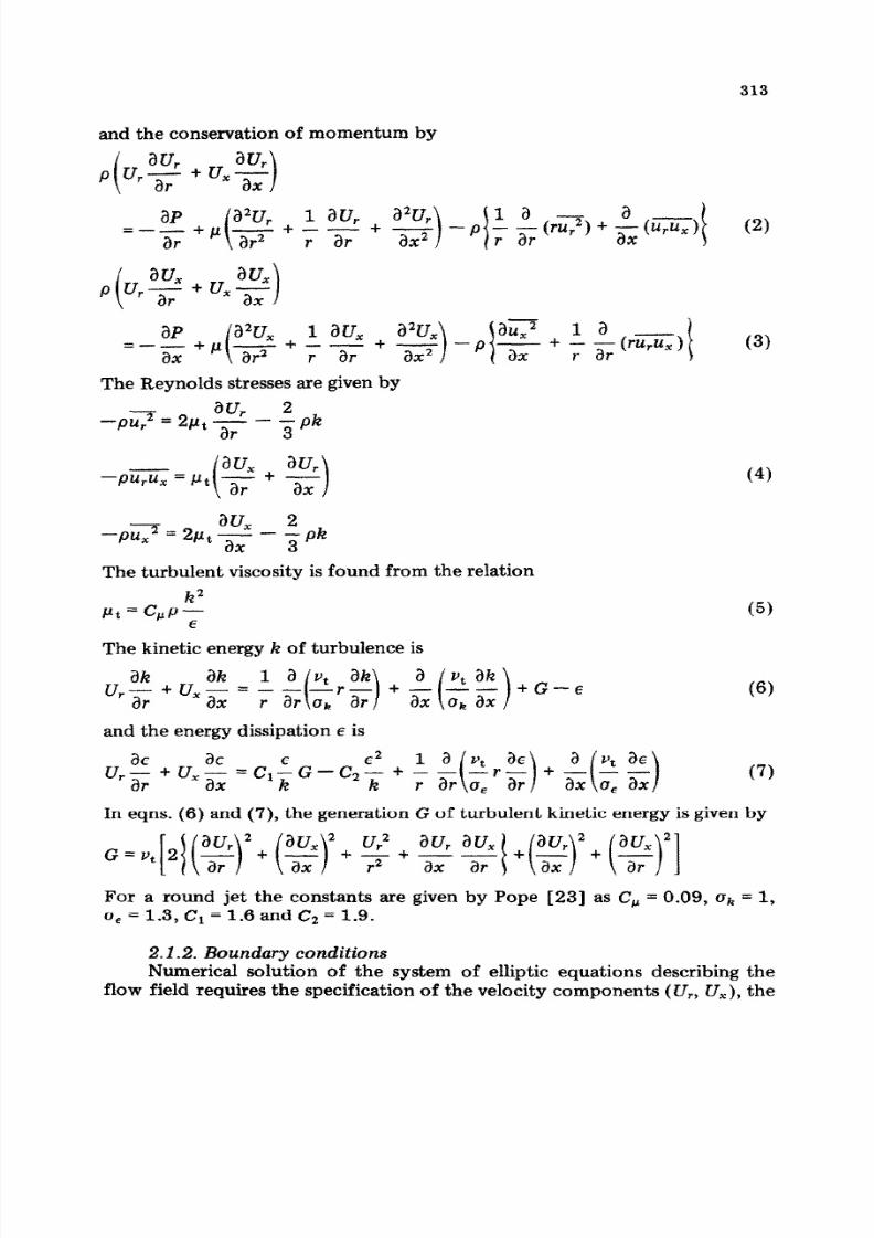
and the conservaticm of momentum by

au, av;

P G$- -I-U”ax

P

The Reynolds stresses are given by

au,-pz = 2/.iEr, x

The turbulent viscosity is found from the relation

h2Pt - C&lPT

The kinetic energy k of turbulence is

and the energy di~ipation E is

(6)

(7)

In eqns. (6) and (7), the generation G of turbulent kinetic energy is given by

For a round jet the constants are given by Pope 1231 as C, = 0.09, ok = 1,

u, = 1.3, C1 = 1.6 and Cz = 1.9.

2.1.2. Boundary conditions

Numerical solution of the system of elliptic equations describing theflow field requires the specification of the velocity components (U,, U, ), the



314

turbulent kinetic energy k and its rate E of dissipation on a closed boundary

(see Fig. 1). The following conditions are used.

(a) Values for all the variables are prescribed at the jet inlet plane. For

r <d/2, U, is the measured value, U,. = 0, k = 0.01Ux2 and E = k3’2/0.2d. Forr > d/2, U, is the measured value (approximately 0), U, = 0, k = 0 and c = 0.

(b) On the axis of symmetry, a(any variable)/& = 0, except for U?

which is equal to zero.

(c) On the wall, V, = 0. The shear stress on the wall was prescribed

from the log~ithmic law of the wall velocity distribution. The values of k

and E were set at the grid points nearest the wall. If it is assumed that the

flow in the wall region is in local equilibrium, the transport equation for k

gives this quantity as a function of the wall shear stress and known quantities

in the flow (see ref. 22). The value of e was set by assuming that near the

wall the length scale for turbulent motion varies linearly with the distance

from the wall.

(d) Araujo et al. [Zl] indicate that the flow in the wall jet region is

approximately parallel to the wall. Hence, on the exit-flow plane, U, = 0,

~~~U~)/~r= 0, ~k ~a~ = 0 and ae,Qr = 0.

2.1.3. Finit e difference equations and num erical solut ion

The equations are discretized by control, or cell, volume integration

over a staggered interconnected grid. The general form of the resulting finite

difference equation for an arbitrary field variable @at a node p in the calcu-lation domain is

where EA& represents both the diffusion and the convection from the

nodes adjacent to the node p, S, and S, represent the sources and sinks of

the quantity 6. The system of difference equations generated by writing

eqn. (8) for the variable 4 at each node p in the calculation domain is readily

solved using the Thomas algorithm.

In the approximation leading to eqn. (8), a hybrid scheme is used todifference the convective terms. In this scheme, when diffusion dominates

convection, central differencing is used for the convective terms. However,

in regions of the flow where convection dominates diffusion, backwards

differencing is used for the convective terms. Because this procedure sacri-

fices accuracy for stability, it is necessary to ensure that a sufficiently

refined grid is used to reduce truncation error to an acceptable level. The

diffusion terms in the equations are always discretized using central dif-

ferencing.

The numerical solution procedure is based on the twodimensional

TEACH code (see, for example, ref. 24). In this procedure, the pressure field

requires special attention. Linearized expressions for the ve1ocit.y com-

ponents, in terms of pressure differences, are substituted into the continuity

equation. The resulting difference equation is solved for pressure using the



315

SIMPLE scheme described by Patankar 125 1. The numerical solution se-quence is as follows. From an initial guess of the flow field (pressure andvelocity) the modified ~ont~uity equation is solved for a better estimate

of the pressure field. Using the updated pressure field, the momentumequations are solved for the velocity components. This is followed by thesolution of k and e from their respective equations in order to obtain abetter estimate of the turbulent viscosity pt. The solution sequence isrepeated until a pre-established convergence criterion is met, this being thatthe sum of the normalized residuals for each variable be less than 10V3.Space considerations have dictated the briefness of this section. However,much information is available on the TEACH code and the numerical prac-tices it embodies. The interested reader will find the reference by Patankar[ 253 especially informative,

2.1.4. Calculation grid

After the dependence of the numerical solution on the refinement anddistribution of the grid was explored, the 49 X 49 unevenly spaced gridshown in Fig. 2 was used for the fluid flow calculations. The spacing be-tween successive grid points differed by a multiplicative constant c. Givenna grid points along the 3c direction, the fo~owing algorithm fixed theirlocation:

Xl = -0.5 Ax

x2 = 0.5 Ax

x, = x,__~ + c”--~ AWL

Fig. 2. Calculation grid.



316

X, = x,_~ + cm-4 Ax

where Ax is determined from the requirement that the computation domain

along x be of length X.x = i(x, +x,-I)

=L. “-4,,+~m_12c

1-cm-4 +

I_ p-3

= + 0.5 Ax2 l-c i

In the axial direction, the constant c was chosen to be 0.95 while in the

radial direction c = 1.058.

The final calculation grid was chosen by increasing the grid refinement

until the calculated fluid field was in good agreement with the experimental

results of Araujo et al. [211. Because of the thinness of both the developing

jet and the wall jet, the grid points were concentrated near the axis of

symmetry and near the wall. Estimates of false diffusion, relative to turbu-

lent diffusion, showed that pfaise/fit < 0.05 in the region of strongest. stream-

line curvature.

2.2. Particle phase

With the fluid flow field determined, it is possible to calculate the

motion of the pa_rticles. A detailed discussion of the relative magnitudes ofthe forces acting on an individual particle has been given by Laitone [20].

Laitone shows that for high speed incompressible air flows in which the

particulate phase is dilute the dominant force acting on a particle is the

drag force. Particle-particle interactions, virtual mass effects, lift, viscous,

pressure, gravity, Basset and Magnus forces are all relatively small and are

assumed to be negligible,

22.1. Equ ation of m otion

The particles are assumed to be spherical so that Stokes’ drag formula

can be used. Since this formula is only valid when the particle Reynoldsnumber (based on the relative velocity between the two phases) is much less

than unity, an empirically determined correction factor f is used when the

particle Reynolds number is of order unity or larger. For the conditions

stipulated, the particle equation of motion is

d2r f-=-dt2 T

(9)

where r = r(xp , p) refers to the position of the particle, the particle velocity

is U, = dr/dt and U is the velocity of the fluid at r. The particle response

time is given by



317

The cor rect ion factor f given by Booth royd [261 is

1

1 + 0.15Re,0*687 O<Re,<200

f =, 0.914Re, o*282 O.O135Re, 200 < Re, G 2500 01)

O.O167Re, Re, > 2500

wher e Re, is th e pa rt icle Reynolds nu mber . Equa tion (9) can be rewr itt en

as a set of first -ord er differen t~ equa tions:

dr-=dt

u*

dUP=

-Qu- p)dt r

(12)

(13)

The solution of t his init ial-value problem requ ires the specificat ion of the

initia l position an d velocity of th e par ticle.

2.2.2. Solution algorithm

One of th e second -ord er Run ge-Kut ta schemes, th e midpoint met hod,

was us ed to solve eqns. (12) an d (13). The midpoint met hod is a mu ltist ep

techn ique in which th e slopes ar e evalua ted at the midpoint of th e time

interval (t,, tn+l). A det ailed discussion of th e midpoint met hod is con-

ta ined in most element ar y nu merical a na lysis textbooks (see, for example,ref. 27). The solut ion algorit hm is as follows (th e super scripts refer to th e

time step).

The first st ep is to determ ine th e position an d the velocity of th e

part icle at t ime t, + h/2. Thus,

hrn+l’2=rn + -p*”

u P n+1/2 xc r/,n + _1 f (U” - Up”)

(14)

When deter min ing th e position an d velocity of th e pa rt icle at tim e t, + h, the

slopes a re evaluat ed a t time t, + h/Z:

r n+l. = r” + hupn+lf2

hfn+1/2 (15)

UPn+Lqpn+

-(Un+1/2 _u n +l/Z

P )7

The t ru ncat ion err or of th is met hod is of ord er h2. The ~plementationof higher order discretizat ion schem es did n ot a lter th e calculat ed p a r t i c l e

trajectories.

The time step h was decreased until further decreases in the time step

did not alter th e solution. A typical time st ep used was lo-' .


http://slidepdf.com/reader/full/httpwwwsciencedirectcomscienceobmiamiimageurlcid271461user512776pii0043164885901759… 10/22

318

22.3. Particle impact velocity

To find the impact velocity, Euler’s method was used to discretize

eqns. (12) and (13). The primary reason for choosing this discretization

scheme was that it facilitates computing the time at which a partiele col-lides with the wall. If a particle collides with the wall during the time step

iz + 1, the location s and the velocity 4 of the particle at the moment of

impact can be determined from

s=r”+KU P (16)

q=U/+Kf”(U”-Up”)7

(17)

The time K at which the collision takes place can be determined using the

x component of eqn. (16) by noting that x, = L at the moment of impact.

2.2.4. Interpolating the fluid velocity

Since the fluid velocity is calculated at fixed grid points using an

eulerian formulation of the equations of motion, the fluid velocity along

the trajectory of a particle must be found by interpolation. Figure 3 shows

the four fluid velocity calculation grid points ((i,j), (i,j + l), (i + 1,j) and

(i + 1, j + 1)) nearest a particle located at (xP, r,). The variables A i (with

i = 1,2,3,4) represent the areas shown in the figure.

A linear interpolation for the fluid velocity around the point (x,, rp) is

given by

wxv d =AlUi+l.j + AzUi,j + AsUi+l,j+l +A~ui j+l

I

EAi(18)

In order to use eqn. (18), the grid point (i, j) must be found (given the

location of the particle).

i , i + 1 i + l , j + l

Fig. 3. The four fluid flow calculation grid points ((i,]), (i,j + I), (i + 1, j) and (i + 1,

.i + 1)) nearest the particle located at (x,, rP). The variables A; represent the areas used in

the weighting scheme given by eqn. (18).



Solving for the grid point number n from the calculation grid relations,

i - 2 = intlog{1 - (1 c)(3tP/A~ - 0.5))

log c 1j- = intlog{1 - (1 c)(rPfAr - 0.5))

log c 1 cw

where the int(x) function takes the integer portion of x.

3. The model for erosion

Given the velocity r~ at which the particles strike the wall surface, theangle 8 at which they strike (measured with respect to the perpendicular tothe surface) and the number N of particles (per area per time) hitting thesurface, the cutting model proposed by Finnie [9,28] can be used to predictthe erosion of a ductile metal plate. In the model, Q is the volume of materialremoved per unit time per unit area by N particles each of mass m. Therelations derived by Finnie are

Nmq*Q=_...m_2p J/ {sin(20) - 3 cos*0}

sfor 71.5” < 8 < 90”

and (21)Nmq*

Qc- sin20 for 0” < B < 71.5”@‘&

Since relative rates of erosion are of interest here, precise values for thewear model constants P and $J are not required. In deriving these equationsFinnie assumed that the fluid phase was of low density and low viscosity(e.g. air) and also that the abrasives strike the metallic surface with a sharpleading edge.

Throughout the remainder of this paper, q, 8 and N are referred to as

the erosion parameters.

4. Results and discussion

4.1. Single-phase impinging jet

For testing purposes, predictions of a single-phase fluid flow field werefirst made for conditions of the experiment of Araujo et al. [21], corre-sponding to an air jet impinging on a smooth wall. Araujo et aE, used laserDoppler ~emomet~ to measure the mean and ~uctuating velocity com-ponents in the free jet and wall jet regions. They made measurements in jetsimpinging both normally and obliquely, with impingement angles rangingfrom 0 = 0” to 8 = 20”. The predictions discussed below were made for anormal impingement angle (0 = 0”).



tc1 Y/r

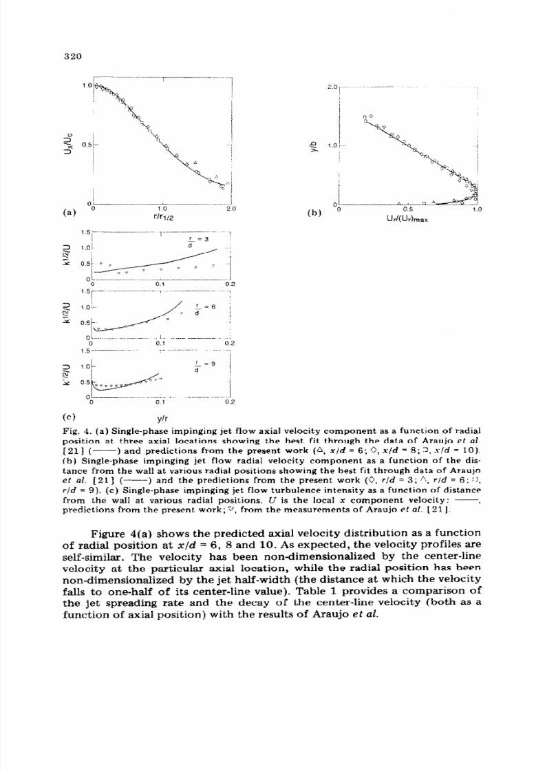
Fig, 4. (a) Single-phase impinging jet flow axial velocity component as a function of radial

position at three axial locations showing the best fit through the data of Araujo et al.

[ 2 1 1 ( ) and predictions from the present work (a, x/d = 6: 9, x/d = 8; 3, s/d = IO).

(b) Single-phase impinging jet flow radial velocity component as a function of the distame from the wall at various radial positions showing the best fit through data of Araujo

et al. [Zl] ( -) and the predictions from the present work (0, r/d = 3; “., r/d = 6; :I,

r/d = 9). (c) Single-phase impinging jet flow turbulence intensity as a function of distance

from the wall at various radial positions. U is the local x component velocity: -,

predictions from the present work; 7’. from the measurements of Araujo at of. f 21 J.

Figure 4(a) shows the predicted axial velocity distribution as a function

of radial position at x/d = 6, 8 and 10. As expected, the velocity profiles are

self-similar. The velocity has been non-dimensionalized by the center-line

velocity at the particular axial location, while the radial position has been

Nan-dimension~ized by the jet half-width (the distance at which the velocity

falls to one-half of its center-line value). Table 1 provides a comparison of

the jet spreading rate and the decay of the center-line velocity (both as a

function of axial position) with the results of Araujo et al.



321

TABLE 1

xld

0

4

6

a

10

The width of the jet ~2rl~~ld~ The center-line uelocity (Ue/Uinf

Araujo et al. Predictions Arcmjo et al. Predictions

1.00 1.00 1.00 1.00

1.17 1.23 0.98 0.99

1.20 1.26 0.93 0.93

1.40 1.42 0.81 0.85

1.69 1.61 0.70 0.72

Figure 4(b) shows the radial velocity as a function of the distance from

the wall at various positions in the wall jet. Both the me~~ernen~ and thepredictions show that the velocity profiles are self-similar. In the figure, thevelocity has been non-dimensionalized by the maximum velocity in the waI1jet (at the radial position in question) and the distance from the wall by thewidth of the wall jet (defined by Araujo eE al. as the distance at which thevelocity falls to one-half the maximum velocity).

Figure 4(c) shows the turbulence intensity as a function of the distancefrom the wall at various radial positions along the wall,

For the purposes of this study, the predictions are in acceptable agree-ment with the experimental results.

4.2. Tkuo-phase impinging jet

The two-phase calculations presented and discussed in this section wereobtained with fluid flow conditions set to the normal impingement jetconfiguration of Araujo et at. discussed above,

4.2.1. Cold gas flowThe effects of various parameters, such as the inlet turbulence intensity

and the particle size, on the motion of sand-like particles (&Jpf = 1709) inair at 300 K are discussed in this section.

Figures 5(a) and 5(b) show the effect of turbulence on the speed Q atwhich 5 pm particles strike the wall surface, the angle 0 at which they strike(measured from the normal to the wall) and the number N of particles (perarea per time) that hit the surface.

The greater the inlet turbulence intensity, the more mixing occurs inthe jet and consequently the faster the jet spreading rate. The conservationof mass requires that the center-line velocities decrease faster. Thus, thegreater the turbulence, the smaller the speeds of impact (as is shown inFig. 5(a)).

Let us consider a fixed radial position on the wall. For the high turbu-lence case, the particles striking the wall at that position originated at apoint closer to the center of the nozzle. Thus, the angle 8 at which theparticles strike the wall increases with increasing turbulence intensity (as isshown in Fig. 5(b)). This point is illustrated schematically in Fig. 5(c).



322

(b)

(cl

Fig. 5. (a) Effect of inlet tu rbu fenee int ensit y on th e impa ct velocity of 5 ,um par ticles

(x = 0.41) in an air jet with Rej = 20 000, H /d = 12 and pPfpf = 1709 for var ious values of

(k”2/U)i~. (b) Effect of inlet tu rbulence intens ity on part icle impact a ngle an d sur face

“flux” for 5 p pa rt icles fh = 0.41) in an air jet with Rej = 20 000, N/d = 12 an d ~~~~~ =

1709. (c) Qualita tive sketch of th e effect of inlet turbu lence intens ity on par ticle tr ajec-

tories.

If it is assumed that the inlet particle flux Ni, is uniform across the

nozzle, the number of particles (per area per time) striking the surface at a

given location decreases with increasing turbulence intensity (see Fig. 5(b)).

The number of particles striking the area nrc2 per unit time is nra2Ni, for the

high turbulence case and nri,‘Ni,, for the low turbulence case (r, is the

impact radial location).

Figure 6(a) shows the effect of particle size on particle trajectory.

Figures 6(b) and 6(c) show the various erosion parameters for 5, 10 and

20 E.tm particles. The results confirm that the motion of larger particles is

relatively unimpeded; thus they strike the surface at greater speeds and at

smaller angles.



323

s 0.5Fluid etnemline

(a) 2 r/d

60

00 1 .o 2.0

2rld

0

fbf ’

1,O

2 rid

Fig, 6. (a) E ffect of part icle size (or moment um equilibrat ion par am eter h) on part icle

tr ajectories in an air jet. All par ticles wer e released from th e sam e initial ra dial position at

th e inlet pla ne (x/d = 0). Flow condit ions ar e Rej = 20 000, H/d = 12, pp/pf = 1709 and

(k”*/U)in = 0.30. (b) Effect of pa rt icle size (or momen tu m equilibra tion par am ete r h)

on impa ct velocity in a n a ir jet with Rej =: 20000, H/d = 12, ppJpf = 1709 and

(Jz~/~/U)~, = 0.30. All pa rt icle sizes had t he sam e inIet m ass flow ra te. (c) Effect of

par ticle size (or momentu m equilibrat ion par am eter k) on impa ct an gle an d sur face flux

in an air jet wit h Rej = 20 000, H /d = 12, &,/pf = 1709 and (k”“/U)in = 0.30. All pa rt icle

sizes had th e same inlet m ass flow ra te, an d Nin for t he 5 pm par ticles ha s been used for

nondimension~ization.

A non-dimensional particle response time or momentum equilibrationconstant h is useful when quantifying the sensitivity of a particle to changesin the mean fluid flow. It is indicated in Fig. 6 and is defined as

ruinX=-..--d

w%?-4,=--181.1 d

The quantity h is the ratio between a time scale characteristic of the meanparticle motion and a time scale characteristic of the mean fluid flow. Theresults of this study are in good agreement with Laitone’s [ZO] prediction



324

that for X G 0.1 the particles follow the streamlines and very few collide with

the wall, whereas for h > 10 the particles are virtually unaffected by the mean

fluid flow. Since this study is concerned with the effects of fluid mechanics

on erosion, particles with response times in the range 0.1 < h < 10 wereinvestigated. For the conditions of this study, 5 pm, 10 pm and 20 pm

particles correspond to response times of 0.41,1.64 and 6.55 respectively.

4.22. Hot gas flow

Figure 7 shows the effect of temperature on the erosion parameters for

10 I.tm particles (p, = 2000 kg mW3) in an air jet with U, = 30 m ss’~ In one

test case the air was at 1200 K (Rej = 2000) and in the other test case it

was at 300 K (Rej = 20 000). In each case, the system was assumed to be

isothermal so that heat transfer between phases could be ignored. The

primary effects of increasing the temperature are to increase the viscosityand to decrease the density of the air. The viscosity increases by a factor of

2.5 and the kinematic viscosity by a factor of 10.

The increase in temperature decreases h by a factor of 2.5. Thus, the

particles follow the fluid more closely.

For the same configuration and the same inlet velocity, the Reynolds

number for the hot gas is smaller by a factor of 10. Thus, the hotter jet will

tend to spread slightly faster and consequently the conservation of mass

requires the axial velocity to decrease faster.All these consequences, due to increasing the temperature of the flow

system, tend to decrease the speed of impact, to increase the angle at which

the particles strike the surface and to decrease the number of particles

striking the surface per area per time at a given position on the plate.

m

fb) 2 r /d

Fig. 7. (a) Effect of tem pera tu re on th e impa ct velocity of 10 pm par ticles. At 300 K,Rei = 20 000 (Vi, = 30 m s-l), A= 1.64 and pp/pf = 1709. At 1200 K, Rej = 2000 (Vi, =

30 m s-l), X = 0.66 an d pP /pi = 6840. In addit ion, H/d = 12 and (k”2/U)i, = 0.30. (b)

Effect of tempera tu re on t he impact an gle and surface flux of 10 pm pa rt icles. Flow

condit ions ar e as given in (a).



325

4.2.3. Liquid flow

Figure 8 shows the erosion parameters for 200 pm (h = 0.587) and

400 pm (h = 2.35) sand-like particles (pp/& = 2) in a water jet with an inlet

velocity of 1.25 m s-i co~esponding to Rel = 20 000. As expected, the

larger particles strike the surface at greater speeds and smaller impact angles.

In liquid flows, as in gas flows, particles corresponding to h = 0.1 follow thestreamlines while particles with h > 10 are virtually unaffected by theturning flow. Because of the assumptions in the particle motion equation,these findings are of qualitative value only.

5B

(a)

(A = 0.587)

0 1I I

02%

2.0

m

(b) 2 r/d

Fig. 8. (a) Effect of particle size (OF momentum equil ibration parameter A) on impactvelocity in a water jet with Rej = 20 000, H/d = 12, pp /& = 2 and (klf2/U)i~ = 0.30. (b)Effect of particle size (or momentum equil ibration parameter h) on impact angle andsurface flux in a water jet with Rej = 20 000, H/d = 12, &,/pf = 2 and (k”2/U)in = 0.30.

Nin far the 5 /tm particles has been used for non-dimensionalization.

4.3. Applications t o surface erosion by particle impact

Figure 9 shows the effect of turbulence on erosion by 5 lum particles(pp/pt = 1709) in an air jet at a temperature of 300 K. Finnie’s f9, 231

ductile metal erosion model was used to illustrate the influence of turbulent

diffusion on erosion.The figure shows a decrease in the amount of erosion with increasing

turbulence intensity. Although perhaps counterintuitive, the phenomenon

can be explained and is due to two effects. One effect is that the impactvelocity decreases with increasing turbulence intensity (see Fig. 5(a)), the

other effect is that the number of particles (per area per time) striking thesurface also decreases with increasing turbulence intensity (see Fig. 5(b)).

Figure 9 also shows that the position of maximum wear is significantlyaffected and is moved nearer the symmetry axis with increasing turbulenceintensity. This is due to the fact that, according to the erosion model,maximum wear occurs at approximately 8 = 74”. Since the line 8 = 74” inFig. 5(b) intersects the high turbulence intensity impact angle curves at small



326

0 1.0 20

2 r/d

Fig. 9. Effect of turbulence intensity on the wear of a ductile metal by 5 pm particles

(h = 0.41)inanair jet with Rej = 20 000, H/d = 12 and pp/pf = 1709. Finnie’s [ZS] modelwas used to calculate the erosion.

values of r, the location of maximum wear is moved progressively closer to

the symmetry axis with increasing turbulence intensity.

In concluding this section attention is drawn to two points. First, the

radial wear patterns implied by the shapes of the profiles in Fig. 9 are in

good qualitative agreement with the patterns observed experimentally by Li

et al. [12] and Benchaita et al. [131. In the case of ref. 12, the experimental

conditions were Rej = 3700 - 12 500, H/d = 12, ,op/pf = 2.4 and X = 10 - 50,while in ref. 13, Rej = 140 000, H/d = 2.5, pp/pf = 2.4 and X = 7 - 30. For a

jet oriented normal to the test specimen surface these workers observed

erosion at the stagnation point, a feature not predicted by the wear model

chosen here for illustration. However, there is very good agreement with the

radial location for maximum wear which was 2r/d = 0.9 in Li et al. [ 121,

2r/d = 0.75 - 0.9 in Benchaita et al. [13] and 2r/d = 0.8 - 1.2 in the present

work. Interestingly, the potential flow model of Benchaita et al. overpredicts

the experimental location of maximum erosion by about 50% for large

values of X. We attribute this discrepancy partly to the inability of their

model to account for turbulent diffusion of momentum along the shearlayer evolving from the nozzle edge (see also Fig. 9). As explained earlier,

turbulent diffusion works to move the location of maximum wear nearer the

wall surface stagnation point.

The second point relates to the first and is offered here as an explana-

tion for the “halo” effect discussed by, among others, Lapides and Levy

[29]. These workers find that the test specimens from jet impingement tests

show two regions of substantially different erosion characteristics. In the

center of the erosion area large amounts of material are removed by the

impacting particles. Surrounding this heavily eroded zone is an annulus of

considerably less-damaged surface, but which still shows clear signs of

particle impact. With reference to Fig. 1 we see that for small values of H/d

the test specimen surface will sense two types of flow. One type is highly

monodirectional and is of large speed in the potential core of the jet. The



327

other type, of lower speed, is embedded in the shear layer generated at thenozzle edge. Relative to the core flow, the shear layer is highly turbulent,

with diffusion working to deviate particle trajectories from their original

paths in a random manner. We suggest that the halo arises as a consequence

of the shear layer surrounding the potential core of the jet and that the sharpdistinction between the halo and the heavily eroded central region should

diminish do~stre~ of the location where the potential core ceases to

exist. Experiments are currently underway in our laboratory which willhelp to confirm or disprove this hypothesis.

5. Conclusions and r~ ommendations

Although limited by the simplifications made in the analysis, thepresent numerical study demonstrates the following.

(1) Fluid turbulence can have a significant influence on erosion by

particle impact in jet flow con~~ations.(2) Numerical methods and physical models are available for predicting

the approximate mean motion and trajectories of particles suspended inturbulent flow. Some of the restrictions imposed in this study can readilybe removed; for example, by including two-way coupling between the phasesand allowing for various particle sizes. Other restrictions, due to particle-particle and particle-wall interactions, are not so easily removed.

(3) The erosion parameters Q, 8 and N vary significantly with fluidtemperature.

Because of the simplicity of the model, the present study demonstra~sthe relative effects of turbulence on erosion on a qualitative basis. The lackof accurate experimental data to guide theoretical developments and to test

predictive numerical models in general has imposed the modest objectives ofthis study. However, from the results provided it is clear that in futureexperiments, aimed at qu~tifying p~icle-fluid motions near surfaces anderosive wear, it will be indispensable to measure and control the turbulent

characteristics of the flows investigated. This will ensure that the charac-teristics of erosion associated with turbulent flow are separated from (as

opposed to confounded with) the ch~ac~ristics more directly associatedwith material properties and particle-surface mechanical interactions.

Acknowledgments

This work was funded by the Technical Coordination Staff of theOffice of Fossil Energy of the U.S. Department of Energy, under Contract

DE-AC03-76SF00098 and through the Fossil Energy Materials Program,Oak Ridge National Laboratory, Oak Ridge, TN. The authors are grateful tothe agency for its support. Thanks are due to Mrs. Judy Reed and Ms. Loris

Donahue for the preparation of this manuscript. The authors’ names appearin alphabetical order.



328

References

1 I. Finnie, Erosion by solid particles in a fluid stream, Symp. on Erosion and Cavita-

tion, in ASTMSpec. Tech. Publ. 307, 1961, pp. 70 - 82 (ASTM, Philadelphia, PA).2 G. M. Faeth, Recent advances in modeling particle transport properties and dispersion

in turbulent flow, Proc. ASME-JSME Thermal Engineering Joint Conf.. Vol. 2,

American Society of Mechanical Engineers, New York, 1983, pp. 517 - 534.

3 J. S. Shuen, A. S. P. Solomon, Q.-F. Zhang and G. M. Faeth, Structure of particle-

laden jets: measurements and predictions, AIAA 22nd Aerospace Sciences Meet.,

Reno, NV, 1984, Paper AIAA-84-0038.

4 W. K. Melville and K. N. C. Bray, The two-phase turbulent jet, Int. J. Heat Mass

Transfer, 22 (1979) 279 - 287.

5 R. S. Crowder, J. W. Daily and J. A. C. Humphrey, Numerical calculation of particle

dispersion in a turbulent mixing layer flow, J. Pipelines, 4 (1984) 159 - 169.

6 F. Pourahmadi and J. A. C. Humphrey, Modeling solid-fluid turbulent flows with

application to predicting erosive wear, Physicochem. Hydrodyn., 4 (3) (1983) 191

219.

7 W. K. Melville and K. N. C. Bray, A model of the two-phase turbulent jet, Inf. J. Heat

Mass Transfer, 22 (1979) 647 - 656.

8 G. P. Tilly, Erosion caused by the impact of solid particles, Treatise Mater. Sci.

Technol., 13 (1979) 287 - 319.

9 I. Finnie, An experimental study of erosion, Proc. Sot. Erp. Stress Anal., 17 (2)

(1959) 65 - 70.

10 I. Finnie, J. Wolak and Y. Kabil, Erosion of metals by solid particles, J. Mater., 2 (3)

(1967) 682 - 700.

11 J. Wolak, P. Worm, I. Patterson and J. Bodvia, Parameters affecting the velocity of

particles in an abrasive jet, ASME Winter Annu. Meet., New York, December 5 IO,1976, Paper 76-WA/Mat-6.

12 S. K.-K. Li, J. A. C. Humphrey and A. V. Levy, Erosive wear of ductile metals by a

particle-laden high velocity liquid jet, Wear, 73 (1981) 295 - 309.

13 M. T. Benchaita, P. Griffith and E. Rabinowicz, Erosion of a metallic plate by solid

particles entrained in a liquid jet, J. Eng. Ind., 105 (1983) 215 - 222.

14 J. 0. Hinze, Turbulent fluid and particle interaction, Prog. Heat Mass Transfer, 6

(1972) 433 - 452.

15 I. Finnie, Some observations on the erosion of ductile metals, Wear, 19 (1972)

81 - 90.

16 D. Mills and J. S. Mason, Learning to live with erosion of bends, 1st Int. Conf. on the

Internal and External Protection of Pipes, University of Durham, September 9 II,

1975, BHRA Fluid Engineering, Cranfield, Paper Gl, pp. Gl-1 - Gl-18.17 I. Finnie, A. Levy and D. H. McFadden, Fundamental mechanisms of the erosive wear

of ductile metals by solid particles. In W. F. Adler (ed.), Erosion: Prevention and

Useful Applications, in ASTM Spec. Tech. Publ. 664, 1979, pp. 36 - 58 (ASTM,

Philadelphia, PA).

18 W. F. Adler, Assessment of the state of knowledge pertaining to solid particle erosion,

Final Rep., 1979 (U.S. Army Research Office, Contract DSAAG29-077-C-0039).

19 J. Laitone, Aerodynamic effects in the erosion process, Rep. LBL-8962, 1979 (Mate-

rials and Molecular Research Division, Lawrence Berkeley Laboratory, University of

California, Berkeley, CA).

20 J. Laitone, Separation effects in gas-particle flows at high Reynolds numbers, Ph.D.

Thesis, University of California, Berkeley, CA, 1979.

21 S. R. B. Araujo, D. F. G. Durao and F. J. C. Firmino, Jets impinging normally andobliquely to a wall, AGARD Conf. on Fluid Dynamics of Jets with Applications to

V/STOL, 1982, Prepr. 308.22 B. E. Launder and D. B. Spalding, The numerical computation of turbulent flows,

Comp. Methods Appl. Mech. Eng., 3 (1974) 269 - 289.



329

23 S. B. Pope, An explanation of the turbulent round-jet/plane-jet anomaly, AIAA J.,

16 (3) (1978) 279 - 280.24 A. D. Gosman and F. J. K. Ideriah, TEACH-BE: a general computer program for two-

dimensional, turbulent, recirculating flows; in M. Arnal, Rep. F&f-83-2, 1976 (Depart-ment of Mechanical Engineering, University of California, Berkeley).25 S. V. Patankar, Numerical Heat Transfer and Fluid Flow, Hemisphere, New York,

1980.26 R. G. Boothroyd, Flowing Gas-Solids Suspensions, Chapman and Hall, London,

1971.27 K. E. Atkinson, An Introduction to Numerical Analysis, Wiley, New York, 1978.28 I. Finnie, Erosion of surfaces by solid particles, Wear, 3 (1960) 87 - 103.

29 L. Lapides and A. Levy, The halo eff ect in jet impingement solid particle erosiontesting of ductile metals, Wear, 58 (1980) 301 - 312.

Appendix A: Nomenclature

b

c

c1, c2

c,

d

d,fh

H

i

jk

I(f

4,

P

PS

4

QQref

r

r

1^1/2

Rej

Re,

U&Xu,2

.1X

width of the wall jetgrid spacing expansion co~st~tt~bulen~e model constantsturbulence model constantnozzle diameter

particle diameterdrag force correction factorintention time stepdistance from nozzle tip to wall surfacegrid index in the axial directiongrid index in the radial directionturbulent kinetic energyparticle massnumber of particles per area per time striking the wallparticle flux through the nozzle

mean pressurewear model constantparticle impact velocityvolume of material removed per unit time per unit areaNi,mUi,2/6PsU/, normalization constant

radial coordinate directionvector position of the particlejet half-widthUi,dfVp jet Reynolds’ number

IU-U,ld,/v,

particle Reynolds’ number based on the relativevelocity of the phasesshear stress componentradial stress componentaxial stress component



330

fluid mean (vector) velocityjet center-line velocity (varies with x)

jet velocity at nozzle tip

particle mean (vector) velocityradial component of fluid mean velocityaxial component of fluid mean velocity

axial coordinate direction {pointing toward wall surface)axial coordinate direction (pointing away from wall surface)

Greek symbols

;dissipation of turbulent kinetic energyangle at which the particle strikes the wall (with respect to thenormal to the wall)

h non-Dimensions particle response time

lu fluid phase dynamic viscosity

fJt fluid phase turbulent viscosityV fluid phase kinematic viscosity

P fluid density (pure phase)

P P particle density (pure phase)

ITk, a, “Prandtl” numbers for k and E7 particle response time

J, wear model constant

5%bscrip t s

f fluid phase

max maximum value

P particle phaser radial coordinate directionX axial coordinate direction

http___=miamiimageurl&_cid=271461&_user=512776&_pii=0043164885901759&_check=y&_coverdate=1985-04-15&view=c&wchp=dglbvlv-zskzs&md5=c996cc84276776aae11b6fa5781ad559_1-s2.0-0043164885901759-main...

Documents