huey-wen lin — lat2007@regensburg1 parameter tuning of three-flavor dynamical anisotropic clover...

Huey-Wen Lin — Lat2007@Regensburg 1

Parameter Tuning of Three-Flavor

Dynamical Anisotropic Clover Action

Huey-Wen LinRobert G. Edwards

Balint Joó

Lattice 2007, Regensburg, Germany


Outline

Background/MotivationWhy do we make our life troublesome?

Methodology and SetupHow do we tune them?

Numerical ResultsBelieve it or not

Summary/OutlookCannot wait?


MotivationBeneficial for excited-state physics,

as well as ground-state


Excited-State Physics

Lattice QCD spectrumSuccessfully calculates many ground states (Nature,…)

Nucleon spectrum, on the other hand… not quite

Example: N, P11, S11 spectrum





Difficult to see excited states with current dynamical simulation lattice spacing (~2 GeV)

Anisotropic lattices (at < ax,y,z)

2f Wilson excited baryons in progress





Difficult to see excited states with current dynamical simulation lattice spacing (~2 GeV)

Anisotropic lattices (at < ax,y,z)

2f Wilson excited baryons in progress

Preliminary result at SciDAC All

Hands’ meeting (mπ = 432 MeV)


Example: N-P11 Form Factor

Experiments at Jefferson Laboratory (CLAS), MIT-Bates, LEGS, Mainz, Bonn, GRAAL, and Spring-8Helicity amplitudes are measured (in 10−3 GeV−1/2 units)

One of the major tasks given to Excited Baryon Analysis Center (EBAC)

Many models disagree (a selection are shown below)

Lattice work in progress at JLab


Only Interested in Ground State?

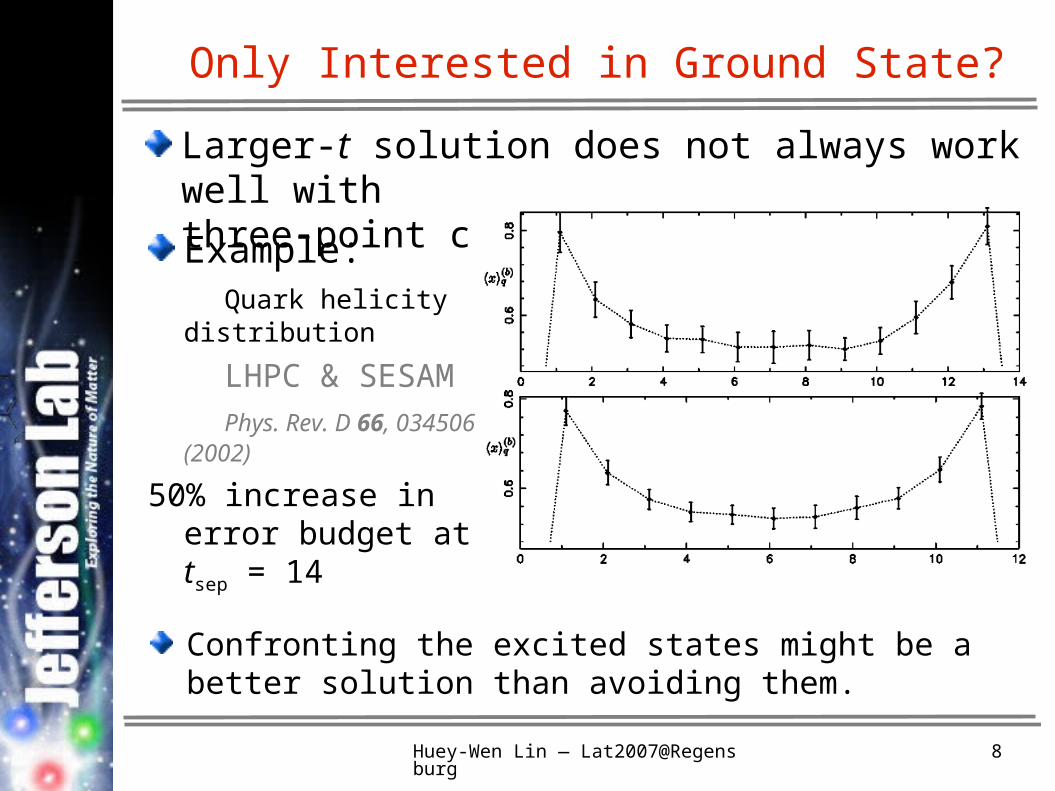
Larger-t solution does not always work well withthree-point correlators

Example: Quark helicity distribution

LHPC & SESAM

Phys. Rev. D 66, 034506 (2002)

50% increase in error budget at tsep = 14

Confronting the excited states might be a better solution than avoiding them.


Methodology and SetupAnisotropic Lattice

+ Schrödinger Functional + Stout-Smearing


Anisotropic Tadpole-ed Lattice Actions

O(a2)-improved Symanzik gauge action

O(a)-improved Wilson fermion (Clover) action

with (P. Chen, 2001)

Coefficients to tune: ξ0, νs, m0 , β


Schrödinger Functional

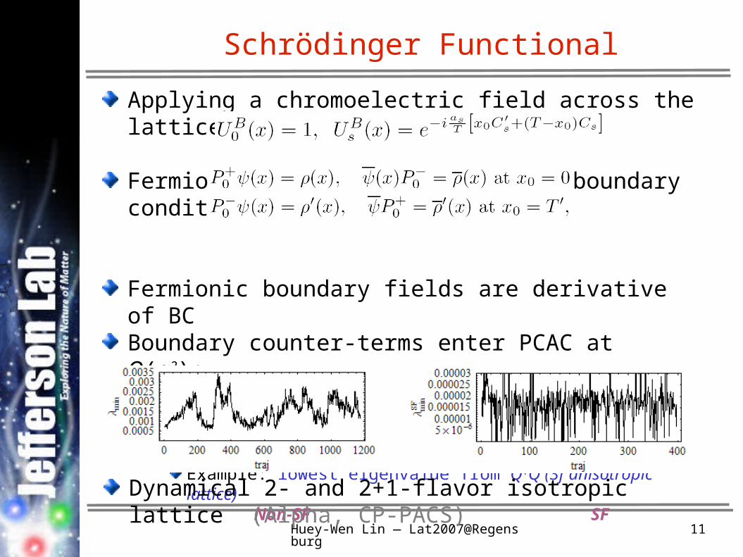
Applying a chromoelectric field across the lattice as

Fermionic sector with additional boundary condition:

Fermionic boundary fields are derivative of BCBoundary counter-terms enter PCAC at O(a2);no further improvement neededBackground field helps with exceptional small eigenvalues

Example: lowest eigenvalue from Q†Q (3f anisotropic lattice)Non-SF SF

Dynamical 2- and 2+1-flavor isotropic lattice (Alpha, CP-PACS)


Isotropic Nonperturbative cSW

O(a) improved axial current

PCAC tells us

Green function with boundary fields

PCAC implies where

Redefined the mass through algebra exercise

with

Nonperturbative cSW from


Stout-Link Smearing Morningstar, Peardon’04

Smoothes out dislocations; impressive glueball results

Better scaling!with n ρ = 2 and ρ = 0.22

Quenched Wilsongauge comparison

Updating spatial links onlyDifferentiable!Direct implementation for dynamical simulation


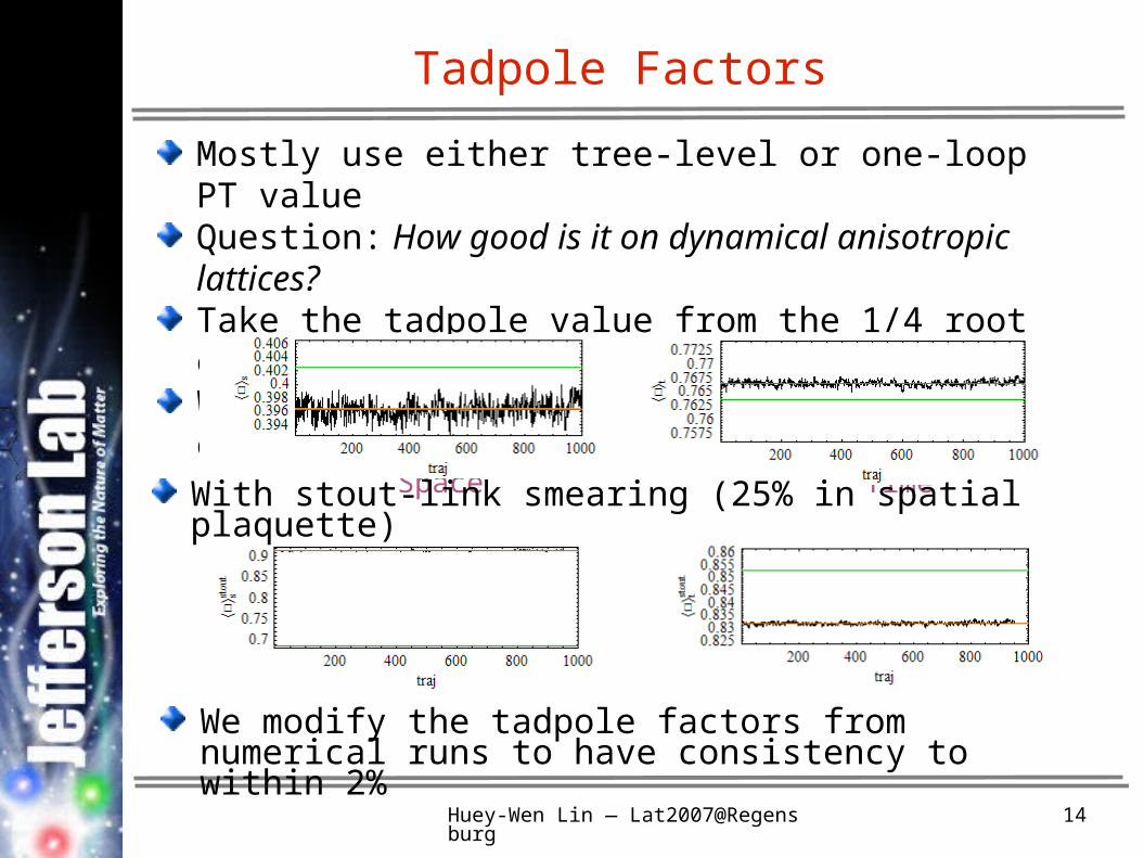
Tadpole Factors

Mostly use either tree-level or one-loop PT valueQuestion: How good is it on dynamical anisotropic lattices?Take the tadpole value from the 1/4 root of the plaquette Without link-smearing (<2% discrepancy is observed)

Space Time

With stout-link smearing (25% in spatial plaquette)Space Time

We modify the tadpole factors from numerical runs to have consistency to within 2%


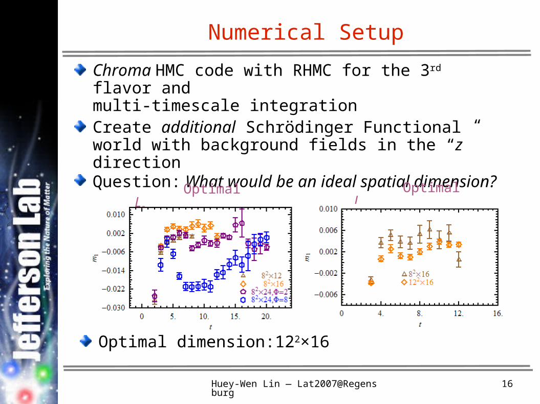
Numerical Setup

Chroma HMC code with RHMC for the 3rd flavor andmulti-timescale integrationCreate additional Schrödinger Functional world with background fields in the “z” directionQuestion: What would be an ideal spatial dimension?

Optimal Lz


Numerical Setup

Chroma HMC code with RHMC for the 3rd flavor andmulti-timescale integrationCreate additional Schrödinger Functional world with background fields in the “z” directionQuestion: What would be an ideal spatial dimension?

Optimal LzOptimal Lx,y

Optimal dimension:122×16


Traditionally, conditions for anisotropic clover actionGauge anisotropy ξ0 ratios of static quark potential (Klassen)

Fermion anisotropy νs meson dispersion relation

The above two are done in the non-SF world, big volume

NP Clover coeffs. (cSW) from PCAC mass difference only in isotropic (Alpha,CP-PACS)

Conditions to Tune

Implement background fields in two directions: t and “z”Proposed conditions:

Gauge anisotropy ξ0 ratios of static quark potential

Fermion anisotropy νs PCAC mass ratioDone in the SF world, small volume

2 Clover coeffs. (cSW) Set to stout-smeared tadpole coefficient

Check the PCAC mass difference


Numerical Results


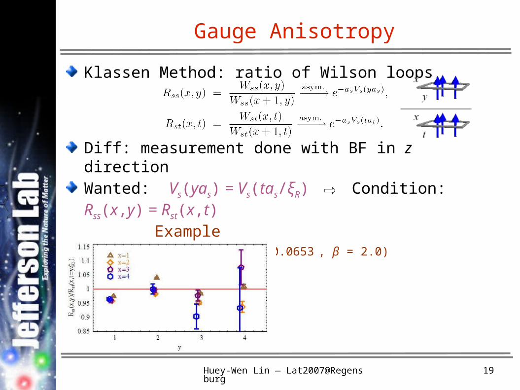
Gauge Anisotropy

Klassen Method: ratio of Wilson loops

Diff: measurement done with BF in z direction Wanted: Vs(yas) = Vs(tas/ξR) ⇨ Condition: Rss(x,y) = Rst(x,t) Example

(ξ0 = 3.5, νs = 2.0, m0 = −0.0653 , β = 2.0)

ξR = 3.50(4)


Gauge Anisotropy

Klassen Method: ratio of Wilson loops

Diff: measurement done with BF in z direction Wanted: Vs(yas) = Vs(tas/ξR) ⇨ Condition: Rss(x,y) = Rst(x,t) Example ξR/ξ0 ≈ 1

(ξ0 = 3.5, νs = 2.0, m0 = −0.0653 , β = 2.0)

ξR = 3.50(4)


2D Parameter/Data Space

Fix ξ0 at 3.5 ➙ ξR ≈ 3.5 Simplify tuning in 2D parameter spaceList of trial parameters




and corresponding data


Fermion Anisotropy

Question: How does our condition for the fermion anisotropy compare with the conventional dispersion relation in large volume?Quick local test:123×128 without background field 3-flavor, m0 = −0.054673, νs = 1.0, as = 0.116(3) fm

From PCAC Ms and Mt,, we see about 10% disagreement


Fermion Anisotropy

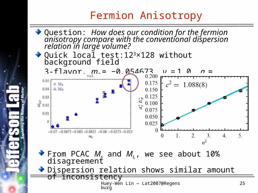
Question: How does our condition for the fermion anisotropy compare with the conventional dispersion relation in large volume?Quick local test:123×128 without background field 3-flavor, m0 = −0.054673, νs = 1.0, as = 0.116(3) fm

From PCAC Ms and Mt,, we see about 10% disagreementDispersion relation shows similar amount of inconsistency


Parameterization

Implement background fields in two directions: t and “z”⇒ 2 PCAC mass, Mt , Ms

Localized region suitable for linear ansatz Ms,t(ν,m0) = bs,t + cs,tν + ds,tm0

Condition: Ms = Mt


Parameterization

Implement background fields in two directions: t and “z”⇒ 2 PCAC masses: Mt , Ms

Localized region suitable for linear ansatz Ms,t(ν,m0) = bs,t + cs,tν + ds,tm0

Condition: Ms = Mt

More runs in the range 0.95 ≤ ν ≤ 1.05 coming


Nonperturbative cSW?

Nonperturbative conditionΔM = M(2T/4,T/4) – M′(2T/4,T/4) = ΔMTree,M=0

Tree-level ΔM value obtained from simulation in free-fieldExamples:

At points where Ms = Mt , the NP condition is satisfied or agrees within σ


Summary/Outlook

Current Status:SF + stout-link smearing show promise in the dynamical runs

Stout-link smearing + modified tadpole factors makeNP csw tuning condition fulfilled

Finite-box tuning is as good as conventional large-box runs with gauge and fermion anisotropy but more efficient

2f anisotropic (ξR = 3) Wilson configurations completed

(L ~ 1.8, 2.6 fm, mπ ~ 400, 600 MeV)

In the near future:Fine tuning the strange quark points

Launch 2+1f, 243 × 64 generation

O(a)-improved coefficients: cV,A, ZV,A…

huey-wen lin — lat2007@regensburg1 parameter tuning of three-flavor dynamical anisotropic clover...

Documents

hueywen lin lat2007

excited states

groundstate slide

progress slide

lattice work

jlab slide

mev slide

nucleon spectrum