human capital in growth regressions: how much …search.oecd.org/economy/outlook/1885692.pdf ·...

Unclassified ECO/WKP(2000)35

Organisation de Coopération et de Développement Economiques OLIS : 12-Oct-2000Organisation for Economic Co-operation and Development Dist. : 20-Oct-2000__________________________________________________________________________________________

English text onlyECONOMICS DEPARTMENT

HUMAN CAPITAL IN GROWTH REGRESSIONS: HOW MUCH DIFFERENCEDOES DATA QUALITY MAKE?

ECONOMICS DEPARTMENT WORKING PAPERS NO. 262

byAngel de la Fuente and Rafael Donénech

Unclassified

EC

O/W

KP

(2000)35E

nglish text only

Most Economics Department Working Papers beginning with No. 144 are now availablethrough OECD’s Internet Web site at http://ww.oecd.org/eco/eco.

96614

Document complet disponible sur OLIS dans son format d’origine

Complete document available on OLIS in its original format

ECO/WKP(2000)35

2

ABSTRACT/RÉSUMÉ

We construct a revised version of the Barro and Lee (1996) data set for a sample of OECDcountries using previously unexploited sources and following a heuristic approach to obtain plausible timeprofiles for attainment levels by removing sharp breaks in the data that seem to reflect changes inclassification criteria. It is then shown that these revised data perform much better than the Barro and Lee(1996) or Nehru et al. (1995) series in a number of growth specifications. We interpret these results as anindication that poor data quality may be behind counterintuitive findings in the recent literature on the(lack of) relationship between educational investment and growth. Using our preferred empiricalspecification, we also show that the contribution of TFP to cross-country productivity differentials issubstantial and that its importance relative to differences in factor stocks increases over time.

JEL Classification: O40, I20, O30

Keywords: human capital, growth

* * * * *

Nous avons révisé l’ensemble des données de Barro et Lee (1996) pour un échantillon de pays del’OCDE, en utilisant des sources auparavant inexploitées, en suivant une approche heuristique afind’obtenir des profils temporels plausibles en ce qui concerne les niveaux d’éducation en supprimant lesruptures importantes dans les séries qui semblent refléter des changements dans les critères declassification. On démontre ensuite que la performance des données révisées est meilleure que celleobtenue en utilisant les séries de Barro et Lee (1996) et de Nehru et al. (1995) dans plusieurs spécificationsde croissance. Nous interprétons ces résultats comme une indication du fait que la mauvaise qualité desdonnées pourrait être à l’origine des résultats contraires à l’intuition dans la littérature récente sur le liennon-significatif entre l’investissement éducatif et la croissance. En utilisant notre spécification empiriquepréférée, nous démontrons également que la contribution de la productivité multifactorielle aux différencesinternationales en matière de productivité est considérable et que son importance relative par rapport auxdifférences en termes de stocks de facteurs augmente avec le temps.

Classification JEL : O40, I20, O30

Mots-clés : capital humain, croissance

Copyright OECD, 2000

Applications for permission to reproduce or translate all, or part of, this material should be made to:Head of Publications Service, OECD, 2, rue André-Pascal, 75775 Paris Cédex 16, France.

ECO/WKP(2000)35

3

TABLE OF CONTENTS

HUMAN CAPITAL IN GROWTH REGRESSIONS: HOW MUCH DIFFERENCEDOES DATA QUALITY MAKE?................................................................................................................. 5

1. Introduction............................................................................................................................................. 52. International data on educational attainment: a brief survey and some worrisome features................... 6

2.1. Educational data bases: coverage and construction.......................................................................... 72.2. A closer look at the OECD data ....................................................................................................... 9

3. Educational attainment in the OECD: A revised set of estimates for 1960-90..................................... 123.1. An example: the case of higher education in Canada..................................................................... 133.2. Some comments on the estimation procedure and data quality...................................................... 143.3. A comparison with the B&L data set ............................................................................................. 15

4. Some empirical results .......................................................................................................................... 164.1. How much difference does data quality make?.............................................................................. 164.2. Is there a trend problem? ................................................................................................................ 184.3. Cross-country differences in TFP levels and the explanatory power of the neo-classical model .. 18

5. Conclusion ............................................................................................................................................ 20

APPENDIX .................................................................................................................................................. 39

1. Detailed country notes .......................................................................................................................... 39United States.......................................................................................................................................... 39Netherlands............................................................................................................................................ 39Italy........................................................................................................................................................ 39Belgium ................................................................................................................................................. 40Spain...................................................................................................................................................... 40Greece.................................................................................................................................................... 40Portugal ................................................................................................................................................. 40France .................................................................................................................................................... 41Ireland.................................................................................................................................................... 41Sweden .................................................................................................................................................. 42Norway .................................................................................................................................................. 42Denmark ................................................................................................................................................ 43Finland................................................................................................................................................... 43Japan...................................................................................................................................................... 44New Zealand.......................................................................................................................................... 44United Kingdom .................................................................................................................................... 45Switzerland............................................................................................................................................ 45Austria ................................................................................................................................................... 45Australia ................................................................................................................................................ 46Germany ................................................................................................................................................ 46Canada ................................................................................................................................................... 47

2. Data tables............................................................................................................................................. 473. Estimation of the stock of physical capital ........................................................................................... 47

BIBLIOGRAPHY......................................................................................................................................... 64

ECO/WKP(2000)35

4

Tables

1. Correlation among alternative estimates of average schooling2. B&L (1996) and NSD versus OECD (EAG), Educational attainment of the adult population3. Attainment levels and codes4. Available data and higher attainment estimates, Canada5. Some summary measures of data quality6. Cumulative years of schooling by educational level7. Average years of schooling around 19908. A production function in levels9. A production function in first differences with and without a catch-up effect10. Results without period dummies, D&D data11. 1985 relative TFP levels, D&D versus K&R12. 1990 relative TFP levels, D&D versus Jones13. Correlations across TFP and productivity measuresA.1 University attainment levelsA.2 Secondary attainment levelsA.3 Illiteracy ratesA.4 Average years of schoolingA.5 Data sources and construction, university attainmentA.6 Data sources and construction, secondary attainmentA.7 Data sources and construction, illiterates (LO)

Figures

1. Average years of schooling in 1985: B&L (1996) versus NSD2. Average years of schooling by level in the OECD: B&L (1996) versus NSD3. Evolution of university attainment levels, Australia, New Zealand and Canada4. Evolution of secondary attainment levels, Netherlands, New Zealand and Canada5. University attainment in Canada, Barro and Lee (1996) versus this paper6. Range of the growth rate of average years of schooling: B&L versus this paper7. Normalised average years of schooling: B&L versus this paper8. Change in normalised average years of schooling between this paper and B&L9. Estimated coefficient of human capital and 95 per cent confidence interval around it when

deleting one country at a time from the sample10. Average growth rates of productivity, per worker factor stocks and the TFP gap and

investment rates in physical and human capital11. Relative productivity versus relative TFP in 196012. Relative productivity versus relative TFP in 199013. Fraction of the productivity differential with the average explained by the TFP gap

in an average country in the sampleA.1 Average years of schooling of population 25 years and overA.2 Percentage of population 25 years and over with primary educationA.3 Percentage of population 25 years and over with secondary educationA.4 Percentage of population 25 years and over with higher education

ECO/WKP(2000)35

5

HUMAN CAPITAL IN GROWTH REGRESSIONS:HOW MUCH DIFFERENCE DOES DATA QUALITY MAKE?

by

Angel de la Fuente and Rafael Donénech1

1. Introduction

1. Recent empirical investigations of the contribution of human capital accumulation to economicgrowth have often produced discouraging results. Educational variables frequently turn out to beinsignificant or to have the “wrong” sign in growth regressions, particularly when these are estimated usingfirst-differenced or panel specifications. The accumulation of such negative results in the recent literaturehas fuelled a growing scepticism on the role of schooling in the growth process, and has even led someresearchers (notably Pritchett, 1995) to seriously consider possible reasons why the contribution ofeducational investment to productivity growth may actually be negative.

2. In this paper we argue that counterintuitive results on human capital and growth may be due, atleast in part, to deficiencies in the data or inadequacies of the econometric specification. When we comparethe different studies in the recent empirical literature on human capital and growth, perhaps the clearestregularity we find is that results are typically much better when we focus on cross-section or pooled dataestimates, and get considerably worse when we consider the results of first-differenced, fixed effects orwithin specifications -- which rely more heavily on the time-series variation of the data.2 To put it in aslightly different way, the data seem to be telling us that, controlling for other things, more educatedcountries do tend to be more productive than others, but that it is not true that productivity rises over timewith human capital in the manner suggested by the cross-section profile.

3. This pattern of results, which is not unusual in panel data estimation,3 may reflect a number of(not mutually exclusive) problems that have nothing to do with the ineffectiveness of educationalinvestment. One possibility is measurement error. If human capital stocks have been measured with error 1. Angel de la Fuente is from the Instituto de Análisis Económico (CSIC) and the CEPR, Rafael Doménech is

from the Universidad de Valencia. This paper is part of a research project co-financed by the EuropeanFund for Regional Development and Fundación Caixa Galicia. The authors gratefully acknowledgeadditional support from the Spanish Ministry of Education through CICYT grants SEC99-1189 andSEC99-0820 and the European TNR “Specialisation vs. diversification: the microeconomics of regionaldevelopment and the propagation of macroeconomic shocks in Europe”. We thank José Emilio Boscá,Anna Borkowsky (Swiss Federal Statistical Office) and Gunilla Dahlen (Statistics Sweden) for theirhelpful comments and suggestions, and María Jesús Freire and Juan Antonio Duro for their helpfulresearch assistance.

2. See among others Mankiw, Romer and Weil (1992), Knight, Loayza and Villanueva (1993), Benhabib andSpiegel (1994), Barro and Lee (1994), Islam (1995), Caselli et al. (1996) and Hamilton and Monteagudo(1998). De la Fuente (2000) surveys this literature.

3. See for example Griliches and Hausman (1986).

ECO/WKP(2000)35

6

(and, as we will argue below, we have every reason to believe this is the case), their first differences willbe even less accurate than their levels, a fact that could explain their lack of significance in some of therelevant studies. A second possibility has to do with the trends of the human capital variables and thegrowth rate of output. Since productivity growth has declined over time while both enrolment rates andschooling levels rose sharply in the last decades (especially in developing countries), a negative sign on thehuman capital variable is not really surprising when we eliminate the cross-section variation of the data,but it may simply reflect the omission of some other factors that may account for the growth slowdown.

4. We provide some evidence that data deficiencies are at least partially responsible for the poorempirical performance of human capital indicators in growth equations. On the other hand, correcting in asimple way for a potential “trends problem” does not significantly affect the results in the OECD samplewe consider when a production function specification is used, although we suspect this may change in abroader sample or with a convergence equation specification.

5. The paper is organised as follows. In Section 2 we briefly review the available data oneducational attainment levels and document some of the problems they display. In Section 3 we describethe construction of new schooling series for a sample of 21 OECD countries. These series are essentially arevised version of (a subset of) Barro and Lee’s (1996) data set that incorporates a greater amount ofnational information than the original series and tries to avoid implausible breaks in the data by correctingfor what appear to be changes in classification criteria. We focus on the OECD in part for reasons of dataavailability and in part because this is the sample for which Mankiw, Romer and Weil (MRW 1992) findweakest support for their human capital-augmented Solow model.4 In Section 4 we show that our reviseddata perform much better than Barro and Lee’s (1996) or Nehru et al.’s (1995) series in a number of fairlystandard growth accounting specifications. Our best results are obtained with a specification in firstdifferences that allows for a technological catch-up effect following de la Fuente (1996). We use thismodel to explore the relative importance of total factor productivity (TFP) and factor stocks as sources ofcross-country productivity differences and find that the contribution of the first factor is substantial andincreasing over time. Section 5 concludes.

2. International data on educational attainment: a brief survey and some worrisome features

6. The basic source of schooling data is a diverse set of indicators provided by national agencies onthe basis of population censuses and educational and labour force surveys. Various internationalorganisations collect this information and compile comparative statistics that provide easily accessible and(supposedly) homogeneous information for a large number of countries. Perhaps the most comprehensiveregular source of international educational statistics is UNESCO’s Statistical Yearbook. This publicationprovides reasonably complete yearly time series on school enrolment rates by level of education for mostcountries in the world and contains some data on the educational attainment of the adult population,government expenditures on education, teacher/pupil ratios and other variables of interest. Other UNESCOpublications contain additional information on educational stocks and flows and some convenientcompilations. Other useful sources include the UN’s Demographic Yearbook, which also reportseducational attainment levels by age group and the IMF’s Government Finance Statistics, which providesdata on public expenditures on education. Finally, the OECD also compiles educational statistics both forits member states (e.g. OECD (1995)) and occasionally for larger groups of countries.

7. The UNESCO enrolment series have been used in a large number of empirical studies of the linkbetween education and productivity. In many cases this choice reflects the easy availability and broadcoverage of these data rather than their theoretical suitability for the purpose of the study. Enrolment rates

4. MRW’s schooling variable is not significant at the usual 5 per cent level in this sub-sample, but does

become significant in broader samples.

ECO/WKP(2000)35

7

can probably be considered an acceptable, although imperfect, proxy for the flow of educationalinvestment. On the other hand, these variables are not necessarily a good indicator of the existing stock ofhuman capital since average educational attainment (which is often the more interesting variable from atheoretical point of view) responds to investment flows only gradually and with a very considerable lag.

8. In an attempt to remedy these shortcomings, a number of researchers have constructed data setsthat attempt to measure directly the educational stock embodied in the population or labour force of largesamples of countries. One of the earliest attempts in this direction is due to Psacharopoulos and Arriagada(PA, 1986) who, drawing on earlier work by Kaneko (1986), report data on the educational composition ofthe labour force in 99 countries and provide estimates of the average years of schooling. In most cases,however, PA provide only one observation per country.

9. More recently, there have been various attempts to construct more complete data sets oneducational attainment that provide broader temporal coverage and can therefore be used in growthaccounting and other empirical exercises. This requires panel data for as many countries and years aspossible.

2.1. Educational data bases: coverage and construction

10. The existing data sets on educational attainment have been constructed by combining theavailable data on attainment levels with the UNESCO enrolment figures to obtain series of average yearsof schooling and the educational composition of the population or labour force. Enrolment data aretransformed into attainment figures through a perpetual inventory method or some short-cut procedure thatattempts to approximate it. We are aware of the following studies:

−� Kyriacou (1991) provides estimates of the average years of schooling of the labour force (h)for a sample of 111 countries. His data cover the period 1965-1985 at five-year intervals. Heuses UNESCO data and PA’s attainment figures to estimate an equation linking h to laggedenrolment rates. This equation is then used to construct an estimate of h for other years andcountries.

−� Lau, Jamison and Louat (1991) and Lau, Bhalla and Louat (1991). These studies use aperpetual inventory method and annual data on enrolment rates to construct estimates ofattainment levels for the working-age population. Their perpetual inventory method uses age-specific survival rates constructed for representative countries in each region but does notseem to correct enrolment rates for dropouts or repeaters. “Early” school enrolment rates areestimates constructed through backward extrapolation of post-1960 figures. They do not useor benchmark against available census figures.

−� Barro and Lee (B&L 1993) construct education indicators combining census data andenrolment rates. To estimate attainment levels in years for which census data are notavailable, they use a combination of interpolation between available census observations(where possible) and a perpetual inventory method that can be used to estimate changes fromnearby (either forward or backward) benchmark observations. Their version of the perpetualinventory method makes use of data on gross enrolments5 and the age composition of the

5. The gross enrolment rate is defined as the ratio between the total number of students enrolled in a given

educational level and the size of the population which, according to its age, “should” be enrolled in thecourse. The net enrolment rate is defined in an analogous manner but counting only those students whobelong to the relevant age group. Hence, older students (typically repeaters) are excluded in this secondcase.

ECO/WKP(2000)35

8

population (to estimate survival rates). The data set contains observations for 129 countriesand covers the period 1960-85 at five-year intervals. Besides the average years of educationof the population over 25, Barro and Lee report information on the fraction of the (male andfemale) population that has reached and completed each educational level. In a more recentpaper (B&L, 1996), the same authors present an update of their previous work. The reviseddatabase, which is constructed following the same procedure as the previous one (except forthe use of net rather than gross enrolment rates), extends the attainment series up to 1990,provides data for the population over 15 years of age and incorporates some new informationon quality indicators such as the pupil/teacher ratio, public educational expenditures perstudent and the length of the school year.

−� Nehru, Swanson and Dubey (NSD 1995) follow roughly the same procedure as Lau,Jamison and Louat (1991) but introduce several improvements. The first one is that Nehruet al. collect a fair amount of enrolment data prior to 1960 and do not therefore need to relyas much on the backward extrapolation of enrolment rates. Secondly, they make someadjustment for grade repetition and dropouts using the limited information available on thesevariables.

11. We can divide these studies into two groups according to whether they make use of both censusattainment data and enrolment series or only the latter. The first set of papers (Kyriacou and Barro andLee) relies on census figures where available and then uses enrolment data to fill in the missing values.Kyriacou’s is the least sophisticated of the two studies. This author uses a simple regression of educationalstocks on lagged flows to estimate the unavailable levels of schooling. This procedure is valid only whenthe relationship between these two variables is stable over time and across countries, which seems unlikelyalthough it may not be a bad rough approximation, particularly within groups of countries with similarpopulation age structures. In principle, Barro and Lee’s procedure should be superior to Kyriacou’sbecause it makes use of more information and does not rely on such strong implicit assumptions. Inaddition, these authors also choose their method for filling in missing observations on the basis of anaccuracy test based on a sample of 30 countries for which relatively complete census data are available.

12. The second group of papers (Louat et al. and Nehru et al.) uses only enrolment data to constructtime series of educational attainment. The version of the perpetual inventory method used in these studiesis a bit more sophisticated than the one in Barro and Lee, particularly in the case of Nehru et al. BothNehru et al. and Louat et al. use estimates of age-specific survival probabilities constructed for arepresentative country in each region. This procedure should be more accurate than Barro and Lee’s roughestimate of survival probabilities (which is not really age-specific and therefore can bias the results ifattainment levels differ significantly across age groups, as seems likely). Unlike Barro and Lee (1993),Nehru et al. also make a potentially important correction for repeaters and dropouts using (limited)country-specific information on these variables.6 On the other hand, these studies completely ignore censusdata on attainment levels. To justify this decision, Nehru et al. observe that census publications typicallydo not report the actual years of schooling of individuals (only whether or not they have completed acertain level of education and/or whether they have started it) and often provide information only for thepopulation aged 25 and over. As a result, there will be some arbitrariness in estimates of average years ofschooling based on this data and the omission of the younger segments of the population may bias theresults, particularly in LDCs, where this age group is typically very large and much more educated thanolder cohorts. While this is certainly true and may call for some adjustment of the census figures on thebasis of other sources, in our opinion it hardly justifies discarding the only direct information available onthe variables of interest.

6. Barro and Lee’s (1996) estimates, however, partially account for these factors by using estimates of net

enrolment rates. The paper, however, gives no details on how net enrolment rates are estimated.

ECO/WKP(2000)35

9

2.2. A closer look at the OECD data

13. Methodological differences across different studies would be of relatively little concern if they allgave us a consistent and reasonable picture of educational attainment levels across countries and theirevolution over time. As we will see presently, this is not the case. Different sources show very significantvariations in terms of the relative positions of different countries. Although the various studies generallycoincide when comparisons are made across broad regions (e.g. the OECD vs. LDCs in variousgeographical areas), the discrepancies are very important when we focus on the group of industrialisedcountries. Another cause for concern is that practically all available data on educational stocks and flows,including UNESCO’s enrolment series, present anomalies which, to some extent, raise doubts about theiraccuracy and consistency. In particular, the schooling levels reported for some countries do not seem veryplausible, while others display extremely large changes in attainment levels over periods as short as fiveyears (particularly at the secondary and tertiary levels) or extremely suspicious trends.7

14. To illustrate these problems and to get some feeling for the overall reasonableness of the existingdata, in this section we will take a closer look at the most sophisticated data sets within each of the groupsof studies identified in the previous section -- i.e. the Barro and Lee (B&L 1996) and Nehru et al. (NSD1995) data sets. As in the empirical section of the paper, we will concentrate on a sample of OECDcountries. One of the main reasons for this choice is that educational statistics for this set of advancedindustrial nations are presumably of decent quality. Any deficiencies we find in them are likely to becompounded in the case of poorer countries.

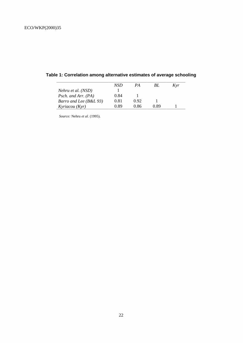
15. The degree of consistency between the various sources varies a lot depending on the level ofaggregation we consider. Table 1, taken from NSD (1995), shows that the overall correlation (computedover common observations) of the different estimates is reasonably high. The correlation between the B&Land NSD figures over the whole sample, for example, stands at a respectable 0.81. An examination ofaverage figures over different geographic regions and over time also reveals a fairly consistent andreasonable pattern. Industrialised countries and socialist economies display much higher attainment ratesthan less developed countries. Within this last group, Africa lies at the bottom, while Latin America doesfairly well and Southeast Asia presents the largest improvement over the period.

16. This high overall correlation, however, hides significant discrepancies between the two data sets,both over time and across countries. Figure 1 shows B&L’s (1996) and NSD’s estimates of the averageyears of total schooling of the population over 15 for OECD countries in 1985. The correlation for the23 countries (there are no data for Luxembourg) is now 0.574, but when we exclude the four countries withthe lowest levels of schooling in the sample, the correlation drops to zero (0.063). When we disaggregate,the correlation is fairly high at the university level (0.767) and much lower for primary (0.362) andsecondary (0.397) attainment.

17. Figure 2 shows the evolution of the average years of total schooling (h) in the average OECDcountry and their breakdown by levels (h1, h2 and h3) according to the same two sources (B&L vs. NSD).If we focus on average years of total schooling, both data sets display an increasing trend, although it ismuch more marked in the case of B&L. In terms of their levels, NSD’s figures on average attainment aresignificantly higher, although the difference between the two sets of estimates diminishes over time andbecomes minor towards the end of the period. In principle, this discrepancy may be due at least in part tothe difference between the age groups considered in the two studies. While B&L focus on the populationaged 15 and over, NSD attempt to measure the educational attainment of the 15 to 64 age group. Since theolder cohorts included in the B&L sample and excluded by NSD are typically less educated than the rest ofthe population, we would expect Barro and Lee’s attainment estimates to be somewhat lower than those inNehru et. al.

7. Behrman and Rosenzweig (1994) discuss some of the shortcomings of UNESCO’s educational data.

ECO/WKP(2000)35

10

18. Significant differences between the two sources emerge when we disaggregate by educationallevel. In terms of secondary schooling the trend is quite similar in both cases but NSD’s estimates are,unexpectedly, lower on average than B&L’s. At the primary level, NSD’s attainment figures areimplausibly high, exceeding the duration of this school cycle (which is around six years on average), anddisplay a downward trend. This “finding” that primary schooling levels have decreased over time inindustrial countries is extremely suspicious, for it implies that new entrants into the labour force have lessprimary schooling than the older generations -- in spite of the rapid increase of enrolment rates over theperiod.

19. For OECD countries we have some alternative sources that can be used to assess the likelyaccuracy of the B&L and NSD series. In particular, the OECD has published some reasonably completeeducational statistics for most of its member countries. Although these data refer only to the last few years,and are not therefore an alternative to the other sources for the statistical analysis of the impact ofeducation on growth, a comparison of the three sets of figures may perhaps give us some clues as to thepossible shortcomings of the B&L and NSD data sets.

20. Table 2 summarises the most relevant data. Notice that although both the year and the age groupsdiffer somewhat across the three sources (see the notes to the table), the figures should be roughlycomparable. The breakdown by educational level is also comparable with the one used by Barro and Lee(1996), although the OECD provides more detail. In particular, they disaggregate secondary attainmentinto two levels and, for most countries, report figures on advanced vocational programmes (ISCED5 level)separately.

21. The differences across the various sources are quite significant. On the whole, the picture whichemerges from the OECD figures seems to be the more plausible one -- at least in the sense of conformingbetter to common perceptions as to the relative educational levels of different countries. As for the othertwo sources, both contain rather implausible features and it is difficult to choose between them. Startingwith the relative positions of different countries in terms of average total schooling (reported in the lastthree columns of the table),8 we find a number of large discrepancies. Barro and Lee’s estimates forAustria, France, Norway and Portugal are much lower than those given in the other sources, while theirfigure for New Zealand is much higher. On the other hand, NSD give very low figures for Australia,Switzerland and Germany, an extremely high estimate for Ireland (which is probably an error) and animplausibly high number for Greece.9 The overall correlation with the OECD estimates is higher for Barroand Lee (0.807) than for NSD (0.531) but this is due to a large extent to the Irish outlier.

22. In the case of Barro and Lee it is possible to make a detailed comparison by levels of schoolingwith the OECD data that may give us some clues as to the likely sources of some of their more implausibleresults. We observe that OECD estimates of secondary attainment are generally higher than Barro and

8. To estimate the average years of schooling on the basis of the OECD data we have used the following

durations: Primary, six years; Secondary I, nine years; Secondary II, 12 years; ISCED 5, 14 years;ISCED 6 and 7, 16 years. Since the computation assumes that everybody who started a certain level hascompleted it, the resulting figures should overstate the true years of schooling but, hopefully, not so muchthe relative positions of the different countries, which is what we are trying to get at. Our comparisons arebased on the standardised attainment figures shown in Table 2, which are constructed by normalising eachestimate of the average years of schooling by the unweighted average of the available contemporaneousobservations in each data set.

9. According to NSD the average years of primary schooling in Ireland ranged between 15 in 1960 and justover 11 in 1985. Both figures are much higher than those for any other country and of the order of twicethe duration of this level of schooling. Greece does not appear in Table 2 because the OECD reports nodata for this country. Greece is ranked by NSD ahead of Switzerland, Australia, Belgium, the Netherlandsand France.

ECO/WKP(2000)35

11

Lee’s.10 The difference exceeds forty points in Austria, Germany, Finland, Denmark, Norway and the UK,and is quite important for a number of other European countries and for Japan. We think the main reasonfor the difference has to do with the treatment of apprenticeships and other vocational trainingprogrammes, which are included in the OECD data but probably not counted by Barro and Lee.Differences in tertiary attainment are significant as well and also seem to be related to the treatment of(higher-level) vocational programmes. In particular, Barro and Lee seem to report ISCED5 studies as partof university schooling but, even accounting for this, significant differences remain in some cases.

23. Turning from the cross-section to the time-series dimension of the data, another disturbingfeature of the human capital series is the existence of sharp breaks and implausible changes in attainmentlevels over very short periods. This problem affects the B&L data set much more than the NSD series,which are much smoother essentially by construction. Figures 3 and 4 below show the evolution of Barroand Lee’s (1996) secondary and university attainment rates for the population over 25 in a number ofcountries that display extremely suspicious patterns. In all cases, the sharp break in the series signals in allprobability a change of criterion in the elaboration of educational statistics. Similar inconsistencies arepresent in other countries as well.

24. The preceding discussion is far from providing an exhaustive list of the suspect features ofdifferent educational data sets. On the other hand, it is probably enough to conclude that --despite the factthat recent contributions represent a significant advance in this area-- the available data on human capitalstocks are still of dubious quality. Remaining problems are probably due in part to the fact that the primarystatistics used in these studies are not consistent, across countries or over time, in their treatment ofvocational and technical training and other courses of study,11 and reflect at times the number of peoplewho have started a certain level of education and, at others, those who have completed it. Additionalproblems may be traced to the procedure used in the construction of the data and even to computationalmistakes. Thus, NSDs neglect of census data probably accounts for their unreasonable results in terms ofthe overall level and trend of primary and secondary schooling while Barro and Lee´s approximation to aperpetual inventory method is probably far from satisfactory. Hence, a fair amount of detailed workremains to be done before we can say with some confidence that we have a reliable and detailed picture ofworldwide educational achievement levels or their evolution over time.

25. To some extent, doubts about the accuracy of existing data sets must raise concerns about thevalidity of the findings of empirical studies based on them. Concerns about data quality, however, alsoadmit an optimistic interpretation of these results. Since there are no reasons to suspect that the availabledata contain systematic biases that may lead us to overestimate the contribution of human capital toproductivity, the fact that the empirical results are quite favourable in some cases in spite of the dubiousquality of the data suggest that improvements in this regard should lead to clearer and more conclusiveresults about education’s contribution to economic growth. We will provide some evidence in this directionbelow.

10. Original OECD figures add up to 100 per cent when we sum primary, secondary and tertiary attainment

rates. Since this implies that everybody has received some schooling, we have corrected the figures usingBarro and Lee’s estimate of the fraction of the population with no schooling. The table reports the originalprimary attainment figure minus the no schooling fraction from Barro and Lee (1996).

11. Steedman (1996) documents the existence of important inconsistencies in the way educational data arecollected in different countries and argues that this problem can significantly distort the measurement ofeducational levels. She notes, for example, that countries differ in the extent to which they reportqualifications not issued directly (or at least recognised) by the state and that practices differ as to theclassification of courses which may be considered borderline between different ISCED levels. Thestringency of the requirements for the granting of various completion degrees also seems to varysignificantly across countries.

ECO/WKP(2000)35

12

3. Educational attainment in the OECD: A revised set of estimates for 1960-90

26. On the basis of our discussion so far we would tentatively conclude that the Barro and Lee (1996)series are probably the best available source on human capital stocks. As we have seen, however, eventhese data contain a large amount of noise that can be traced largely to inconsistencies of the underlyingprimary statistics. Trying to reduce this noise, we have constructed a revised version of the Barro and Leedata set for a sample of 21 OECD countries for the period 1960-90.12

27. We aim to provide estimates of the fraction of the population aged 25 and over that has started(but not necessarily completed) each of the levels of education shown in the upper block of Table 3(illiterates (L0), primary schooling (L1), lower and upper secondary schooling (L2.1 and L2.2) and twolevels of higher education (L3.1 and L3.2)). For some countries, however, the available data may refer to adifferent age group or to the fraction of the population that has completed each schooling level, and it isnot always possible to detect when this is the case.

28. We have tried to include upper-level vocational courses (ISCED 5 studies according to theinternational standard classification of educational attainment levels, L3.1(5) in our notation) in the firstlevel of higher attainment. For some countries the data is detailed enough to allow us to identify thiscategory separately and to recover a narrower, strictly university attainment category (UNIV).13 We reportL0 only for the four countries where illiteracy rates are significant during the sample period (Portugal,Greece, Spain and Italy). For the rest of the sample, the lowest reported category is L1, and it includes allthose who have not reached secondary school.

29. Our approach has been to collect all the information we could find on educational attainment ineach country, both from international publications and from national sources (census and survey resultsand national statistical yearbooks), and use it to try to reconstruct a plausible pattern, reinterpreting someof the data if necessary.14 For those countries for which reasonably complete series are available, we haverelied primarily on national sources. For many of the rest, we start from the most plausible set ofattainment estimates available around 1990 (taken generally from OECD sources) and proceed backwardsusing all the assembled information and trying to avoid unreasonable jumps in the series by choosing themost plausible figure when several are available for the same year, and by reinterpreting some of the data(as referring to broader or narrower schooling categories than the reported one) when it seems sensible todo so. Missing observations are then filled in a variety of ways. Where possible, we interpolate betweenavailable observations. Otherwise, we use information on educational attainment by age group in order tomake backward projections, or rely on miscellaneous information from a variety of sources in order toconstruct plausible estimates of attainment levels. We have avoided the use of flow estimates based onenrolment data because they seem to produce implausible time profiles.

30. Clearly, the construction of our series involves a fair amount of guesswork. Our “methodology”looks decidedly less scientific than the apparently more systematic estimation procedures used by otherauthors starting from supposedly homogeneous data. As discussed in the previous section, however, even acursory examination of the data shows that there is no such homogeneity. Hence, we have found itpreferable to rely on judgement to try to piece together the available information in a coherent manner than

12. The revised series and a detailed description of the estimation procedure are contained in the Appendix.

Iceland, Luxembourg, Turkey and recent OECD members are left out because of the scarcity ofinformation

13. We do not report this finer data except in the case of Canada, where our figures for L3 incorporate atentative estimate of ISCED 5 courses that the user may want to change.

14. We would greatly welcome any additional information that may help us improve the quality of ourestimates, particularly in the case of the more problematic countries cited in Section 3.2.

ECO/WKP(2000)35

13

to take for granted the accuracy of the primary data. The results do, as we will see, look more plausiblethan the existing series, at least in terms of their time profile.

3.1. An example: the case of higher education in Canada

31. To give the reader a flavour for the way our series have been constructed, we will discuss indetail the case of higher education in Canada. This is a country for which there is a considerable amount ofinformation that displays, if taken literally, a rather implausible pattern. It is also one case in which we canpartially check the reasonableness of our corrections for part of the sample period against an apparentlyhomogeneous national source for an age group slightly different from our target.

32. The essence of our approach is captured by Figure 5. The thicker line in the figure describesBarro and Lee’s (1996) higher educational attainment series for the population aged 25 and over, which isbased on UNESCO and UN data. The implausible hump-shaped pattern of the series strongly suggests thatthe 1975 and 1980 observations refer to a broader concept of higher attainment than the rest of the data.Our guess is that, unlike the rest, these two atypical observations include upper-level vocational trainingcourses. If we homogenise the series by consistently including or excluding an estimate of this category,we get the more plausible profile described by the two thinner lines shown in the figure. The higher ofthese lines refers to higher education in a broad sense, and the lower one to strictly university attainment.The dots lying on these two lines represent actual data taken from various sources and attributed to theexact year to which they correspond (and not to the closest multiple of five). For the rest of the years, wecomplete the series through linear interpolation.

33. The details of the reconstruction are unavoidably messy. Table 4 contains the available primarydata and our reconstructed series, with bold characters used to highlight the information we have selectedto construct our estimates. The upper half of the table summarises the university attainment data we havefound for Canada. The sources are various OECD publications (generally for the age group 25-64),UNESCO’s Statistical Yearbook and the UN’s Demographic Yearbook (for the population over 25),national census reports and the web site of Statistics Canada (for the population over 15). UNESCO andthe Demographic Yearbook (DYB) report university attainment as a whole (L3), while national sourcesdistinguish between shorter and longer college-level courses (L3.1 and L3.2). The longer available series,provided by UNESCO and the UN, show considerable discrepancies in some years and (especially in thecase of UNESCO) display a rather implausible pattern that strongly suggests changes in classificationcriteria.

34. Using these data, we have constructed the estimates shown in the lower part of the table. Sincewe suspect changes in the classification of upper level vocational courses are behind the jumps in the data,we distinguish between short university courses (L3.1(6)) and advanced vocational training (L3.1(5)) andconsider various combinations of the three possible categories that comprise higher education: L3 includesall three of them, while UNIV = L3.1(6) + L3.2 includes only strictly university courses, excludingvocational training.

35. Using this finer breakdown, we construct our estimates essentially by trying to guess to which ofthe possible attainment categories the available data refer. We interpret UNESCO’s 1960, 1986 and 1991observations, and the DYB observation for 1975 as referring to university attainment in the narrow sense(i.e. excluding ISCED 5 courses). We complete the series for this attainment level by interpolating betweenavailable observations. Next, we would like to break down university attainment into its upper (L3.2) andlower [L3.1(6)] cycles. For this, we interpret the 1960 DYB figure as referring to L3.2 and estimate L3.2 in1986 and 1991 by applying the ratio L3.2/UNIV computed using the census data (which refers to thepopulation over 15) to our previous estimate of UNIV. To complete the L3.2 and L3.1(6) series we theninterpolate between these three observations.

ECO/WKP(2000)35

14

36. Finally, we need to estimate the level of attainment in advanced vocational programmes and addit to UNIV to obtain total higher attainment (L3). We observe that UNESCO gives extremely high figuresfor university attainment in 1976 and 1981 that we interpret as estimates of L3 [i.e. assume that theyinclude L3.1(5)]. For 1992, OECD (1995) gives a L3 figure that seems compatible with the previous ones.We interpolate L3 between 1981 and 1992 and estimate L3.1(5) as L3 - UNIV, using our previousestimates of these two levels for 1976 onward. To take L3 and L3.1(5) back from 1976, we assume that theratio UNIV/L3 remains constant at its 1976 value. The estimates constructed in this way seem to fit fairlywell with the figures reported in the Statistics Canada web site (for 1976 onward and for the population15+) if we assume that the L3.1 reported in this source includes ISCED 5 courses). These data correspondto the unconnected round dots lying close to the upper line in Figure 5.

3.2. Some comments on the estimation procedure and data quality

37. A similar approach has been followed for the remainder of the sample, as discussed in thedetailed country notes contained in the Appendix. Data availability varies widely across countries. Table 5shows the fraction of the reported data points that are taken from direct observations and the earliest andlatest such observations available for secondary and higher attainment levels. The number of possibleobservations is typically 21 for each level of schooling (two sublevels and a total times seven quinquennialobservations), but it may be larger if the data allow a finer breakdown by sublevel (as in the case ofCanada) or if there is no data close to 1990 and we use observations for around 1995 to complete the series(in which case there is one more time period to consider). In the case of Italy, there seem to be no shorthigher education courses, so the number of possible observations at the university level drops to seven. Wecount as direct observations backward projections constructed using detailed census data on educationalattainment by age group and the age structure of the population.

38. As can be seen in the table, for around two-thirds of the countries we have enough primaryinformation to reconstruct reasonable attainment series covering the whole sample period. The moreproblematic cases are highlighted using bold characters. In the case of Italy, the main problem is that mostof the available information refers to the population over six years of age. We are currently exploring waysto correct the likely bias using data on enrolments and the age structure of the population. For Germanyand Denmark, the earliest available direct observation refers to 1970 or later. We have projected attainmentrates backward to 1960 using the attainment growth rates reported in OECD (1974), but we are unsure ofthe reliability of this extrapolation. Finally, the number of available observations is rather small in thecases of Australia, the UK and Switzerland.

39. A number of countries do not separate primary education from lower secondary schooling andreport a single attainment level that comprises all mandatory courses. To preserve the homogeneity of ourattainment categories, we have estimated the breakdown of compulsory schooling into L1 and L2.1. Forsome countries we have assumed that the ratio L1/L2.1 is the same as in some close neighbour. Inparticular, we have used the value of this ratio in the US to estimate the breakdown in Canada, and appliedthe Swedish ratio to Norway and Denmark. For those countries for which there is no obvious candidate forthis role (Austria, the UK and Switzerland), we have used an ad-hoc regression estimate of the relevantratio. Using the remainder of the sample (except Japan, where the information on L1 and L2.1 is ofdubious quality), we estimate the following equation with pooled data:

L2.1/(L1+ L2.1) = 0.0802 + 0.0094 (L3+L2.2) + 0.1998 (L3/L2.2) - 0.0029*trend adj. R2 = 0.6207 [1] (0.74) (13.25) (4.36) (1.84)

where the numbers in parentheses below each coefficient are t ratios. That is, we hypothesise that thosecountries that are more “efficient” in getting students into the upper schooling cycles will also have greateraccession rates to lower secondary schooling. Hence we specify the weight of lower secondary schooling

ECO/WKP(2000)35

15

relative to primary attainment as a function of university and upper secondary attainment and the ratio ofthe two, and allow it to vary systematically over time. Since the fit of the equation is reasonably good, weuse it to estimate the lower secondary/compulsory attainment ratio in the countries for which thisinformation is not available.

40. Using our attainment series, we finally construct an estimate of the average years of totalschooling for each country and period. The assumed cumulative duration of the different school cycles ineach country is shown in Table 6. In constructing these series we are implicitly assuming that everybodywho starts a given school cycle does eventually complete it, which is clearly not the case. Hence, ourfigures will be biased upward and are not strictly comparable with Barro and Lee’s average schoolingseries, which do incorporate estimates of completion rates.15, 16

3.3. A comparison with the B&L data set

41. Our results differ from Barro and Lee’s original series in two important respects. In the timedimension, the profiles of our attainment series are considerably smoother and more plausible. In the crosssection dimension, there are some significant changes in the relative positions of different countries thatbring us, on average, closer to the pattern found in the OECD sources reviewed in Section 2.2. A detailedcountry by country comparison of the two sets of series can be found in Figures A1-A4 in the Appendix.

42. The importance of eliminating sharp breaks in the series is clearly apparent from Figure 6, whichhas been constructed by arranging the annualised growth rates of the average years of schooling for allperiods and years in decreasing order within each data set. The difference in the range of this variableacross data sets is enormous: while our annual growth rates (D&D) range between 0.15 per cent and 2 percent, Barro and Lee’s go from -1.35 per cent to 7.80 per cent; moreover, 15.9 per cent of their reportedgrowth rates are negative, and 19 per cent of them exceed 2 per cent. We suspect that the excessivevolatility of the Barro and Lee series captured by these figures may be an important part of the reason whythese data often generate implausible results in growth regressions, particularly when these are estimatedusing panel or first difference specifications. The empirical results we report in the following section are,as we will see, consistent with this hypothesis.

43. As we have already noted, our average years of schooling series is not directly comparable withBarro and Lee’s. To examine changes in the cross-section pattern of the data, therefore, we first takeaverages across periods and then normalise both sets of resulting figures so that the unweighted sampleaverage is set equal to 100 in each case. Figures 7 and 8 summarise the differences across data sets in thisnormalised measure of average attainment over the sample period. Figure 7 plots our average attainmentlevels (D&D) against Barro and Lee’s (B&L). As may be expected, the correlation between the two sets offigures is quite high (0.826). There are, however, important deviations from the “diagonal” (i.e. differencesin normalised attainments across data sets) that are reproduced in decreasing order in Figure 8. Relative toBarrro and Lee’s estimates, France and Austria gain almost thirty points and surpass Greece in theattainment ranking, while New Zealand, Denmark and Finland experiment sizeable downward revisions.Table 7 shows the correlation across data sets of average years of schooling around 1990. Our estimates(D&D) are slightly closer to the OECD data than to B&L and display a rather low correlation with NSD’sfigures.

15. The average number of years of schooling in our series (taken across all countries and periods) is 9.29, as

compared with 7.56 for Barro and Lee (1996).

16. The available data on completion rates present the same anomalies we have discussed above in connectionwith attainment and enrolment rates.

ECO/WKP(2000)35

16

4. Some empirical results

44. In this section we examine the performance of our revised data set and Barro and Lee’s andNehru et al’s original series in a number of growth accounting specifications. The results support ourhypothesis that the lack of correlation between productivity growth and human capital accumulationreported in some recent studies may be due to data deficiencies. Using the Barro and Lee data, the partialcorrelation between productivity and educational attainment is only significant in specifications in levels,and the estimated coefficient of human capital in an aggregate production function is quite low in all cases.The results with NSD data are generally even worse: the human capital variable is not significant except inone specification in which its coefficient is negative. With our revised data, in contrast, the coefficient ofhuman capital in an aggregate production function remains positive, significant and large in all thespecifications we consider and, unlike in Mankiw, Romer and Weil (1992), survives a simple robustnesstest. We also explore the possibility that a trend problem may bias the coefficient of human capital ingrowth regressions and use our preferred specification to investigate the contribution of factor stocks andTFP to cross-country productivity differences.

4.1. How much difference does data quality make?

45. The first specification we estimate is a constant-returns aggregate production function in levels,which we write in intensive form,

qit = Γ + γi + ηt + αkit + βhit + εit [2]

where qit is the log of output per employed worker in country i at time t, k the log of the stock of physicalcapital per worker17 and h the log of the average number of years of schooling of the adult population. Weuse dummy variables to capture fixed time and country effects (ηt and γi). In all the results reported belowonly those country dummies that turn out to be significant are left in the equation. The productivity data aretaken from an updated version of Dabán, Doménech and Molinas (1997). We use pooled data at five-yearintervals starting in 1960 and ending in 1990 for B&L and D&D, and in 1985 for NSD.

46. The pattern of results shown in Table 8 is consistent with our hypothesis about the importance ofeducational data quality for growth results. For all three data sets, the coefficient of human capital ispositive in both specifications in levels (with and without fixed country effects), but the size andsignificance of the human capital coefficient increases appreciably as we go from the NSD data to the B&Land D&D data sets. The differences are even sharper when the estimation is repeated with the data in firstdifferences, as in equations [1]-[3] in Table 9, where only our revised data produce a significant (althoughimplausibly large) human capital coefficient. The results obtained with the B&L and NSD data sets areconsistent with those reported by Kyriacou (1991), Benhabib and Spiegel (1994) and Pritchett (1995), whofind insignificant (and sometimes negative) coefficients for human capital in an aggregate productionfunction estimated in first differences.

47. Next, we estimate a catch-up specification along the lines of de la Fuente (1996). The estimatedequation is of the form18

17. See the Appendix for a description of the construction of this variable.

18. We consider an aggregate production function of the form:

Y = Kα(ALH)β(AL)1−α−β

ECO/WKP(2000)35

17

∆qit = Γο + γi + ηt + α∆kit + β∆hit + λbit + εit [3]

where ∆ denotes annual growth rates (over the sub-period starting at time t) and

bit = (qus,t - αkus,t - βhus,t) - (qit - αkit - βhit) [4]

is the Hicks-neutral TFP gap between each country and the US at the beginning of each five-year sub-period. To estimate this specification we substitute [4] into [3] and use NLS with data on both factor stocksand their growth rates. Notice that in this specification the country dummies will pick up permanent cross-country differences in relative TFP levels that will presumably reflect differences in R&D investment andother omitted variables. The parameter λ measures the rate of (conditional) technological convergence.

48. The results are shown in equations [4]-[6] in Table 9. As in previous specifications, the humancapital variable is significant and displays a reasonable coefficient with our revised data, but not with theB&L series or with the NSD data, which actually produce a negative and significant human capitalcoefficient. Moreover, the coefficients of the stocks of physical and human capital estimated with the D&Ddata are quite plausible, with α only slightly above capital’s share in national income and β only slightlybelow Mankiw, Romer and Weil’s (1992) preferred estimate of 1/3.

49. We have checked the robustness of our results by re-estimating our preferred specification (thecatch-up equation labelled [6] in Table 9) for all the possible sub-samples obtained by deleting one countryat a time from the original data set. Figure 9 displays the estimated human capital coefficient and the95 per cent confidence interval around it, after arranging the coefficient estimates in decreasing orderacross sub-samples. As can be seen in the figure, sample composition does not make a significantdifference in terms of the estimated coefficient, and all the estimates remain significantly different fromzero at conventional confidence levels. By contrast, Temple (1998) reports that Mankiw, Romer andWeil’s (1992) proxy for educational investment looses its significance once a few influential observations

Dividing through by employment, rearranging and taking logarithms, log output per employed worker, q,can be written in the form

q = αk + βh + (1-α)a

where k = ln (K/L), a = ln A and h = ln H. We can solve this expression for a as a function of productivityand factor stocks

a = α

βα−

+−�

��

and take growth rates to obtain

∆q = α∆k + β∆h + (1-α)∆a.

Finally, we hypothesise that the rate of technical progress is given by

∆ait = λ(aus,t - ait) + µi + υt

where we have added country and period sub-indices µi and υt are fixed country and period effects. Substituting thislast expression into the production function in growth rates, using the above expression for log TFP andsimplifying, we obtain equation [3] in the text. Notice that in the presence of technological catch-up (λ >0), the technological distance between each country and the leader converges to a constant value. Thisimplies that, asymptotically, all countries display the same rate of technical progress, so the fixed countryeffects µi translate only into differences in TFP levels, and not into permanent differences in growth ratesof TFP.

ECO/WKP(2000)35

18

are removed. In the OECD sub-sample, in particular, the removal of Japan suffices to make the coefficientof the human capital variable insignificant (with a t ratio below one).

4.2. Is there a trend problem?

50. We suspect that the positive trend of human capital investment at a time of slowing productivitygrowth may have also contributed to the lack of significance of educational variables in growth regressionsreported in several studies. As we will see in this section, however, this potential “trends problem” doesnot appear to be important in our OECD sample with our specification, although we suspect that this resultmay not be extensible to data sets that include developing countries or to convergence equations. Even inour sample, moreover, we find that the partial correlation between human capital investment andproductivity growth is not significant in the pooled data unless we control in some way for other factorsthat may be responsible for the productivity slowdown. This can be achieved either by including a set ofperiod dummies or by controlling for the remaining variables suggested by our structural model.

51. Figure 10 summarises the time-series behaviour of the relevant variables. The upper panel of thefigure shows the evolution of the average growth rates (taken across countries) of productivity, factorstocks per worker and the TFP gap. As is well known, the growth rate of productivity declines markedlyduring the period, as does the rate of accumulation of physical capital, while the growth rate of educationalattainment is rather stable. The figure suggests that growth accounting regressions will tend to attribute thegrowth slowdown to the relative decline in investment in physical capital and will not necessarily generatea spurious negative human capital coefficient (as it may be the case if the growth rate of this variabledisplayed an upward trend).

52. To confirm this hypothesis, we have re-estimated several of the specifications in the previoussubsection omitting the period dummies, together with a simple regression of productivity growth onhuman capital accumulation with and without fixed period effects. The results are shown in Table 10.When human capital is the only regressor, its coefficient is only significant when we include perioddummies (see equations [1] and [2] in Table 10). Once we control for the accumulation of physical capital,however, the educational variable becomes significant even without fixed time effects, except in thespecification in first differences without technological catch-up (equation [5]). With this single exception,the results are qualitatively very similar with and without time effects, although the inclusion of perioddummies does tend to reduce marginally the coefficient of physical capital and to increase the coefficientof human capital, except in the last equation.

53. Things are likely to be different, however, with a convergence equation specification à laMankiw, Romer and Weil (MRW 1992). As shown in the lower panel of Figure 10, the rate of investmentin physical capital is relatively stable over the period, while an MRW-style indicator of educationalinvestment (that reflects secondary and university enrolment as a fraction of the adult population) displaysa clear positive trend and will tend to be negatively correlated (over time, although not necessarily acrosscountries) with the growth rate of productivity.

4.3. Cross-country differences in TFP levels and the explanatory power of the neo-classical model

54. A number of authors have recently called attention to the crucial role of technical efficiency inunderstanding productivity disparities across economies and questioned the capacity of the human capital-augmented neo-classical model with a common technology to explain the international or interregionaldistribution of income.19 The catch-up specification we proposed and estimated in a previous section can be 19. See for instance Islam (1995), Caselli et al. (1996), de la Fuente (1996), Jones (1997), Klenow and

Rodriguez (1997) and Prescott (1998).

ECO/WKP(2000)35

19

seen as a further extension of (the technological components of) an augmented neo-classical model thatallows for cross-country differences in TFP levels and for a process of technological diffusion. In thissection, we will use this model to explore the relative importance of differences in TFP levels and in factorstocks as sources of international productivity differentials. The exercise is similar to the one performed byKlenow and Rodriguez-Clare (K&R 1997) but it is conducted using a refined data set that should helpimprove the quality of TFP estimates and an empirically-based set of production function parameters. Inaddition, the examination of the relative TFP levels implied by our regression estimates should be helpfulas a check on the reasonableness of our results, and on the robustness of recent findings by K&R (1997)and Jones (1997).

55. Having estimated our preferred specification (equation [6] in Table 9), we can recover the Hicks-neutral technological gap between each country and a fictional average economy to which we attribute theobserved sample averages of log productivity (q) and log factor stocks per employed worker (k and h).Thus, we define relative TFP (tfprel) by

tfprelit = (qit - αkit - βhit) - (qavit- αkavit - βhavit) = qrelit - (αkrelit + βhrelit) [5]

where av denotes sample averages and rel deviations from them.

56. As may be expected, the correlation between relative productivity and relative TFP is clearlypositive. Figures 11 and 12 show the correlation between these two variables in 1960 and 1990 togetherwith the fitted regression line. Relative productivity is measured along the vertical axis so that the countryranking in terms of TFP levels is more readily apparent. Countries lying above the regression line would bethose where relatively high factor stocks per worker raise productivity above the level expected on thebasis of technical efficiency.

57. Tables 11 and 12 compare our estimates of relative TFPs with those obtained by K&R (1997) for1985 and by Jones (1997) for 1990 and with relative productivity in the same year.20 In each table,countries are arranged in decreasing order of relative productivity (qrel), and the rankings induced by thedifferent variables are shown next to their values. We consider suspicious, and highlight using bold italiccharacters, those cases in which a country’s ranking in terms of TFP is five or more positions away fromits relative productivity ranking. By this criterion, Jones’ estimates yield ten suspicious cases, K&R’sseven, and D&D’s four in 1985 and five in 1990. In spite of these differences, Table 12 shows that thecorrelations across the different TFP estimates and contemporaneous relative productivity levels arereasonably high. This finding may perhaps give us some confidence that, although TFP estimates for agiven country should probably not be taken too literally,21 the overall picture given by our results is notparticularly misleading on average.

58. This is important because we would like to use our results to examine the relative contributionsof TFP gaps and factor stocks to cross-country productivity differences. To obtain a summary measure of

20. Jones (1997) and K&R (1997) report TFPs (Ai) expressed in a Harrod-neutral (labour-augmenting) fashion.

We have converted them into their Hicks-neutral equivalent, which is the appropriate measure for our

calculations, by computing (Ai)1-α with α set to the value used in each of these papers (1/3 for Jones and

0.30 for K&R).

21. There are, indeed, some implausible results in all three papers. Perhaps the biggest surprises are Norway,Switzerland and Spain. We suspect that in the case of Spain part of the problem lies in the fact that theeducational level of the employed workforce (which is a relatively small fraction of the population due tolow participation and high unemployment rates) exceeds that of the adult population by a wider marginthan in other countries. Hence, we are underestimating the relevant stock of human capital and this biasesour estimate of TFP upward.

ECO/WKP(2000)35

20

the relative importance of these two factors, we regress relative TFP on relative productivity. (Notice thatthe regression constant will vanish because both variables are measured in deviations from sample means).The estimated coefficient gives the fraction of the productivity differential with the sample averageexplained by the TFP gap in a “typical country”. Figure 13 shows the evolution of this “average TFPshare” in relative productivity. With our data, this coefficient rises consistently over the sample period,from 0.353 in 1960 to 0.472 in 1990. That is, TFP differences seem to have become relatively moreimportant over time in explaining productivity disparities. Equivalently, this result shows that per workerfactor stocks have been converging faster than efficiency levels, although the behaviour of both variableshas contributed to the narrowing of cross-country productivity differentials.

59. Towards the end of the sample period, one half of the productivity differential with the sampleaverage can be traced back to differences in technical efficiency, with the other half being attributable todifferences in factor stocks. The message is similar if we use K&R’s estimates of the TFP gap, as the TFPshare estimated with these data is 0.495 in 1985.22,23 This result stands approximately half way betweenthose reported by Mankiw (1995), who attributes the bulk of observed income differentials to factorendowments, and those of Caselli et al. (1996) and some other recent panel studies of convergence wherefixed effects that presumably capture TFP differences account for most of the observed cross-countryincome disparities.24 We view these results as an indication that, while the augmented neo-classical modelprevalent in the literature does indeed capture some of the key determinants of productivity, there is a clearneed for additional work on the dynamics and determinants of the level of technical efficiency.

5. Conclusion

60. Existing data on educational attainment contain a considerable amount of noise. Due to changesin classification criteria and other inconsistencies in the primary data, the most widely used series onhuman capital stocks often display implausible time-series and cross-section profiles. After discussing themethodology and contents of these data sets and documenting some of their weaknesses, we haveconstructed new attainment series for a sample of OECD countries. We have attempted to increase thesignal to noise ratio in these data by exploiting a variety of sources not used by previous authors, and byeliminating sharp breaks in the series that can only arise from changes in data collection criteria. While ourestimates unavoidably involve a fair amount of guesswork, we believe that they provide a more reliablepicture of cross-country relative educational attainments and their evolution over time than previouslyavailable data sets.

61. The exercise was originally motivated by the view that weak data was likely to be one of themain reasons for the discouraging results obtained in the recent empirical literature on human capital andgrowth. Our results clearly support this hypothesis. Unlike Barro and Lee’s (1996) or Nehru et al.’s (1995) 22. K&R actually report a higher number (around 2/3), in part because they attribute to TFP differences in

factor endowments that are presumably induced by differences in levels of technical efficiency. In practice,their adjustment amounts to working with the TFP gap in its Harrod-neutral form (without multiplying itby 1-α, which raises its value by about 50 per cent, thereby increasing the share of efficiency in relativeproductivity. By contrast, we consider only the direct contribution of the TFP gap, without trying to guessits indirect effects through induced factor accumulation.

23. Things are somewhat different with Jones’ estimates, which yield a TFP share of only 0.291 in 1990 (asmay have been anticipated by noting the low correlation between Jones’ gaps and relative productivityshown in Table 13). In our view, however, many of Jones’ TFP estimates look rather implausible, makingit dangerous to proceed, as the author does, to use them as the basis for long-term relative income forecasts.

24. If we repeat the exercise with our 1990 data and Caselli et al.’s most “plausible” estimates of theparameters of the production function (α = 0.107 and β = 0.00), the share of TFP in relative productivity inour sample is 0.90.

ECO/WKP(2000)35

21

original series, our revised data produce positive and theoretically plausible results using a variety ofgrowth specifications and, unlike MRW’s original (1992) results for the same sample, our findings survivea simple robustness check.

62. Our preferred specification is a constant returns production function in first differences with atechnological catch-up mechanism and fixed period and country effects. This simple equation explains80 per cent of the variation in the growth rate of productivity and yields sensible technological parametersand generally plausible estimates of cross-country relative TFP levels. We have used this model and theunderlying data to examine the relative importance of differences in factor stocks and levels of technicalefficiency as sources of international productivity differentials. Our results show that the relativeimportance of TFP differences is considerable and that it has increased over time to account for about onehalf of the productivity differentials observed at the end of the sample period. These findings reinforcerecent calls by a number of authors for better models of technical progress as a key ingredient forunderstanding international income dynamics while preserving an important role for factor stocks as asource of cross-country income disparities.

ECO/WKP(2000)35

22

Table 1: Correlation among alternative estimates of average schooling

NSD PA BL KyrNehru et al. (NSD) 1Psch. and Arr. (PA) 0.84 1Barro and Lee (B&L 93) 0.81 0.92 1Kyriacou (Kyr) 0.89 0.86 0.89 1

Source: Nehru et al. (1995).

ECO/WKP(2000)35

23

Table 2: B&L (1996) and NSD vs. OECD (EAG), Educational attainment of the adult populationNo

schoolPRIMARY SEC. I SEC II SECONDARY

TOTALISCED 5 UNIVERSITY

ISC6-7 ISC5-7app/enrsec II

YEARS OF SCHOOLING(avge = 100)

Source = B&L B&L OECD OECD OECD B&L OECD OECD B&L OECD OECD OECD NSD B&L OECDAustralia 2.4 26.6 11.6 30.0 25.0 48.4 55.0 21.0 22.6 10.0 31.0 0.28 84.2 116.7 105.5Austria 2.3 42.5 35.0 60.0 46.9 95.0 0.0 8.4 5.0 5.0 0.37 97.0 85.8 107.6Belgium 1.4 48.4 31.6 30.0 20.0 37.0 50.0 10.0 13.1 7.0 17.0 92.8 100.9 91.8Canada 1.0 15.7 13.0 14.0 41.0 62.0 55.0 15.0 21.4 15.0 30.0 111.0 119.2 110.6Denmark 0.0 38.7 43.0 40.0 41.6 83.0 7.0 19.6 10.0 17.0 0.19 101.3 129.3 108.6Finland 0.0 49.4 42.0 40.0 35.3 82.0 8.0 15.4 10.0 18.0 0.03 108.7 112.9 109.0France 1.2 57.6 22.8 26.0 33.0 28.4 59.0 7.0 12.8 7.0 14.0 0.10 94.3 79.3 94.3W. Germany 2.6 64.9 22.0 61.0 22.0 83.0 7.0 10.4 10.0 17.0 0.59 94.0 101.8 114.6Ireland 4.2 40.4 32.8 25.0 23.0 43.6 48.0 7.0 11.7 7.0 14.0 139.4 94.0 87.6Italy 15.3 44.1 28.7 30.0 20.0 31.7 50.0 0.0 8.9 6.0 6.0 88.1 71.0 75.1Japan 0.0 34.3 30.0 48.0 44.5 78.0 8.0 21.2 13.0 21.0 121.8 106.1 112.5Netherlands 4.0 34.4 15.0 26.0 36.0 45.5 62.0 13.0 16.1 6.0 19.0 0.22 93.4 98.7 99.8New Zealand 0.0 36.8 33.0 10.0 25.0 24.1 35.0 22.0 39.1 9.0 31.0 98.0 128.9 100.4Norway 2.6 49.8 35.0 42.0 32.2 77.0 10.0 15.4 11.0 21.0 105.1 91.4 109.5Portugal 24.4 58.7 64.6 4.0 2.0 11.4 6.0 2.0 5.5 4.0 6.0 63.5 41.6 52.1Spain 4.5 64.4 62.5 13.0 10.0 21.3 23.0 0.0 9.8 9.0 9.0 79.3 72.1 73.0Sweden 2.4 35.4 33.0 44.0 43.9 77.0 11.0 18.4 12.0 23.0 109.2 109.3 113.0Switzerland 6.3 28.5 20.0 50.0 52.3 70.0 15.0 12.9 9.0 24.0 0.68 77.1 102.3 109.4United Kingdom 3.6 43.9 35.0 48.0 38.5 83.0 6.0 13.9 9.0 15.0 113.2 100.3 108.0United States 1.2 9.1 6.8 10.0 46.0 44.4 56.0 12.0 45.2 23.0 35.0 128.7 138.4 117.6Average 4.0 41.2 37.8 61.4 17.1 9.6 18.7 9.0 8.7 10.4

Note: Attainment is measured by the fraction of the adult population which has started (but not necessarily completed) each educational level.Dates and population groups vary as follows: Barro and Lee: 1990 and population aged 25 and over; NSD: 1987 and population aged 15-64; OECD: 1989 andpopulation aged 25-64.The OECD includes apprenticeship programmes as part of secondary (2nd cycle) studies. Level 5 of the international standard classification for education, ISCED 5,includes relatively short post-secondary programmes which do not lead to a university degree. These are generally advanced vocational programmes. Universityprogrammes are included in levels 6 and 7 of ISCED. In some countries which do not report data at the ISCED 5 level, these programmes are counted either at the universitylevel or as part of secondary-level vocational programmes.

ECO/WKP(2000)35

24

Table 3: Attainment levels and codes

Code LevelL0 IlliteratesL1 Primary schoolingL2.1 Lower secondary schoolingL2.2 Upper secondary schoolingL2 Total secondary schooling = L2.1 + L2.2L3.1 Higher education, first cycle or shorter coursesL3.2 Higher education, second cycle or full-length coursesL3 Total higher education = L3.1 + L3.2

L3.1(5) Upper-level vocational courses (Isced 5 level)L3.1(6) Shorter university courses or first cycle (included in Isced 6)UNIV University attainment = L3.1(5) + L3.2

Table 4: Available data and higher attainment estimates, Canada

Source Rep. level 1960 1965 1970 1975 1976 1980 1981 1985 1986 1990 1991 1992OECD L3.1 15 23 26.1OECD L3.2 15 17 15UNESCO L3 13.1 17.8 31.15 37.4 19.3 21.4DY L3 6.5 16 17.3 19.3 19.3 21.4Census L3.1 10.4 11.7Census L3.2 11.5 13.4Stat Can L3.1 24.14 27.65 30.19 31.74Stat Can L3.2 6.43 8.01 9.57 11.36

Estimates 1960 1965 1970 1975 1976 1980 1981 1985 1986 1990 1991 1992L3 25.03 26.88 28.73 30.75 31.15 36.15 37.40 38.75 39.08 40.43 40.76 41.10L3.1(5) 11.93 12.82 13.70 14.66 14.85 18.65 19.60 19.75 19.78 19.45 19.36L3.1(6) 6.60 6.87 7.14 7.49 7.56 8.20 8.36 9.01 9.17 9.81 9.98L3.1.(5+6) 26.10L3.2 6.50 7.20 7.90 8.60 8.74 9.30 9.44 9.99 10.13 11.17 11.42 15.00UNIV =L3.1(6)+L3.2

13.10 14.07 15.03 16.00 16.30 17.50 17.80 19.00 19.30 20.98 21.40

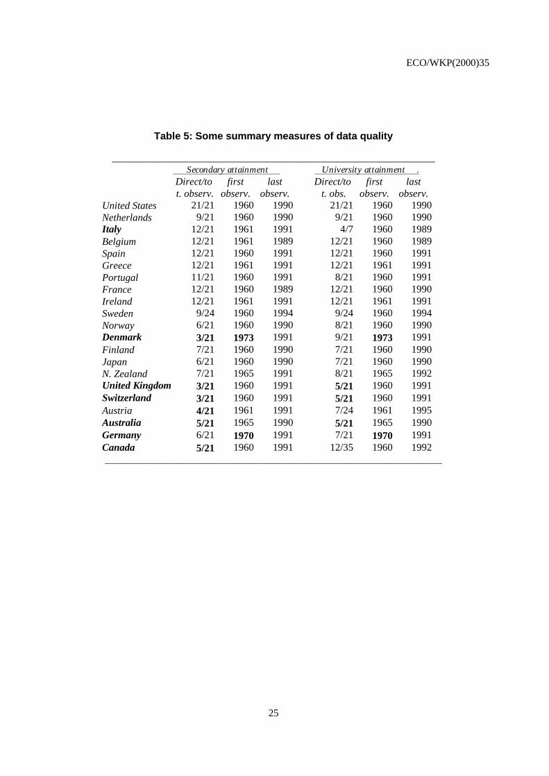
ECO/WKP(2000)35

25

Table 5: Some summary measures of data quality

______________________________________________________________________ Secondary attainment University attainment .

Direct/tot. observ.

firstobserv.

lastobserv.

Direct/tot. obs.

firstobserv.

lastobserv.

United States 21/21 1960 1990 21/21 1960 1990Netherlands 9/21 1960 1990 9/21 1960 1990Italy 12/21 1961 1991 4/7 1960 1989Belgium 12/21 1961 1989 12/21 1960 1989Spain 12/21 1960 1991 12/21 1960 1991Greece 12/21 1961 1991 12/21 1961 1991Portugal 11/21 1960 1991 8/21 1960 1991France 12/21 1960 1989 12/21 1960 1990Ireland 12/21 1961 1991 12/21 1961 1991Sweden 9/24 1960 1994 9/24 1960 1994Norway 6/21 1960 1990 8/21 1960 1990Denmark 3/21 1973 1991 9/21 1973 1991Finland 7/21 1960 1990 7/21 1960 1990Japan 6/21 1960 1990 7/21 1960 1990N. Zealand 7/21 1965 1991 8/21 1965 1992United Kingdom 3/21 1960 1991 5/21 1960 1991Switzerland 3/21 1960 1991 5/21 1960 1991Austria 4/21 1961 1991 7/24 1961 1995Australia 5/21 1965 1990 5/21 1965 1990Germany 6/21 1970 1991 7/21 1970 1991Canada 5/21 1960 1991 12/35 1960 1992_________________________________________________________________________

ECO/WKP(2000)35

26

Table 6: Cumulative years of schooling by educational level

_________________________________________________L1 L2.1 L2.2 L3.1 L3.2

Australia 7 11 13 15 16Austria 6 9 13 15 17Belgium 6 8 12 15 16Canada 6 9 12 15 16Denmark 6 9 13 14 17Finland 6 9 12 14 17France 5 9 12 14 16Germany 4 10 13 15 17Greece 6 9 12 16 16Ireland 6 9 12 14 16Italy 5 8 13 15 18Japan 6 9 12 14 16Netherlands 6 10 12 16 17Norway 6 9 12 14 16New Zealand 6 11 13 15 16Portugal 6 8 12 14 16Spain 5 8 12 14 17Sweden 6 9 12 14 16Switzerland 6 9 13 16 17United Kingdom 6 9 12 14 16United States 7 10 12 14 16Mode 6 9 12 14 16

_______________________________________________________Source Education at a Glance 1997 (OECD, 1998), except figures in bold type (WDI,

World Bank, 1999) and in italics (national sources). These figures are combinedwith our attainment series to estimate the average number of years of totalschooling reported in Table A.4 in the Appendix.

Table 7: Average years of schooling around 1990

Correlation across data sets_________________________________________

NSD B&L OECDB&L 0.542OECD 0.531 0.807D&D 0.355 0.797 0.871

_________________________________________

Note: Same data as in Table 2, except for D&D. Greece is notincluded for lack of OECD data.

ECO/WKP(2000)35

27

Table 8: A production function in levels

___________________________________________________________________________[1] [2] [3] [4] [5] [6]

Human cap.Variable

NSD B&L D&D NSD B&L D&D

α 0.607 0.560 0.516 0.565 0.552 0.567(18.23) (14.73) (13.92) (27.21) (25.95) (20.53)

β 0.069 0.112 0.269 0.088 0.120 0.279(1.69) (3.21) (4.88) (1.80) (6.48) (7.52)

Adj. R2 0.873 0.885 0.896 0.981 0.978 0.979Std. Error reg. 0.136 0.131 0.124 0.053 0.057 0.056Country dummies no no no yes Yes yesPeriod dummies yes yes yes yes Yes yes

___________________________________________________________________________

Note: White’s heteroscedasticity-consistent t ratios in parentheses below each coefficient. Only significantcountry dummies are left in the reported equation. Human capital is measured by the average yearsof total schooling in each country and period. D&D refers to this paper.

Table 9: A production function in first differences with and without a catch-up effect

___________________________________________________________________________[1] [2] [3] [4] [5] [6]

Human cap.variable

NSD B&L D&D NSD B&L D&D

α 0.519 0.508 0.493 0.510 0.409 0.373(9.66) (9.51) (9.21) (8.30) (6.12) (7.15)

β 0.090 0.063 0.493 -0.148 -0.057 0.271(0.80) (1.03) (2.04) (2.62) (0.88) (2.53)

λ 0.100 0.063 0.068(6.98) (8.27) (6.34)

Adj. R2 0.719 0.710 0.718 0.840 0.811 0.809Std. error reg. 0.0098 0.0097 0.0096 0.0074 0.0079 0.0079Country dummies no no no yes yes yesCatch-up effect no no no yes yes yesPeriod dummies yes yes yes yes yes yes

___________________________________________________________________________

Note: White’s heteroscedasticity-consistent t ratios in parentheses below each coefficient. Only significantcountry dummies are left in the reported equation.

ECO/WKP(2000)35

28

Table 10: Results without period dummies, D&D data

___________________________________________________________________________[1] [2] [3] [4] [5] [6]

Human cap.Variable

D&D D&D D&D D&D D&D D&D

α 0.579 0.604 0.544 0.294(24.95) (38.19) (11.27) (6.67)

β 0.683 1.21 0.236 0.247 0.090 0.328(1.56) (3.92) (4.44) (6.93) (0.36) (3.22)

λ 0.076(7.04)

Adj. R2 0.011 0.396 0.894 0.977 0.664 0.785Std. error reg. 0.018 0.014 0.125 0.058 0.0105 0.0084Country dummies no no no yes no yesCatch-up effect no no no no no yesPeriod dummies no yes no no no noData in diff. diff. levels levels diff. diff.

___________________________________________________________________________

Note: White’s heteroscedasticity-consistent t ratios in parentheses below each coefficient. Only significantcountry dummies are left in the reported equation.

Table 11: 1985 relative TFP levels, D&D vs. K&R

______________________________________________________________________ This paper K&R (1997) .

Qrel ranking Tfprel 85 ranking tfprel 85 rankingUnited States 0.325 1 0.183 2 0.152 4Belgium 0.251 2 0.203 1 0.030 9Netherlands 0.179 3 0.105 5 0.138 5Switzerland 0.164 4 -0.009 11 -0.004 10Germany 0.135 5 -0.006 9 -0.013 12France 0.134 6 0.083 7 0.179 3Italy 0.133 7 0.158 4 0.179 2Canada 0.125 8 0.088 6 0.186 1Austria 0.052 9 -0.008 10 0.062 7Norway 0.045 10 -0.110 19 -0.013 13Australia 0.008 11 -0.055 14 0.038 8Spain -0.001 12 0.170 3 0.101 6Denmark -0.021 13 -0.053 13 -0.139 17United Kingdom -0.069 14 0.032 8 -0.013 11Japan -0.088 15 -0.090 17 -0.171 20Ireland -0.120 16 -0.047 12 -0.050 15Sweden -0.126 17 -0.081 15 -0.031 14New Zealand -0.153 18 -0.098 18 -0.118 16Finland -0.170 19 -0.194 21 -0.150 19Greece -0.254 20 -0.086 16 -0.150 18Portugal -0.545 21 -0.183 20 -0.206 21

______________________________________________________________________

ECO/WKP(2000)35

29

Table 12: 1990 relative TFP levels, D&D vs. Jones

______________________________________________________________________ This paper Jones (1997) .

qrel Ranking Tfprel 90 ranking tfprel 90 RankingUnited States 0.281 1 0.157 4 0.017 11Belgium 0.262 2 0.230 1 0.087 7Italy 0.179 3 0.186 2 0.222 1France 0.167 4 0.114 5 0.182 3Germany 0.145 5 0.022 9 0.030 10Netherlands 0.138 6 0.089 6 0.104 4Switzerland 0.084 7 -0.074 13 0.010 12Austria 0.082 8 0.018 10 0.104 5Canada 0.070 9 0.023 8 0.050 9Norway 0.037 10 -0.136 20 -0.140 17Spain -0.011 11 0.165 3 0.197 2Japan -0.018 12 -0.058 12 -0.166 19Ireland -0.026 13 0.049 7 -0.003 13Denmark -0.052 14 -0.096 14 -0.193 20Australia -0.073 15 -0.107 17 -0.076 15United Kingdom -0.086 16 0.018 11 0.081 8Finland -0.114 17 -0.157 21 -0.140 18Sweden -0.152 18 -0.104 16 -0.024 14New Zealand -0.156 19 -0.133 19 -0.324 21Greece -0.281 20 -0.103 15 -0.132 16Portugal -0.482 21 -0.109 18 0.104 6

______________________________________________________________________

Table 13: Correlations across TFP and productivity measures

______________________________________________________________________________TFP85D&D TFP85K&R TFP90D&D TFPP90J

QREL85 0.775 0.773 QREL90 0.711 0.370TFP85D&D 0.824 TFP90D&D 0.750

______________________________________________________________________________

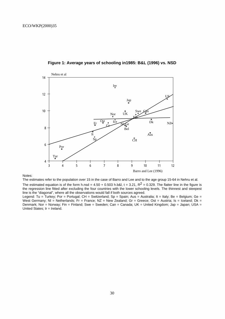
ECO/WKP(2000)35

30

Figure 1: Average years of schooling in1985: B&L (1996) vs. NSD

3 4 5 6 7 8 9 10 11 124

6

8

10

12

14

Tur

Por

Ire

Sp

It

US

NZ

CH

Aus

Dk

Can

Jap

FrOst

Nor

GrIce

Bel

Nl-Ge

UKSwe

Fin

Barro and Lee (1996)

Nehru et al

Notes:The estimates refer to the population over 15 in the case of Barro and Lee and to the age group 15-64 in Nehru et al.

The estimated equation is of the form h.nsd = 4.50 + 0.503 h.b&l, t = 3.21, R2 = 0.329. The flatter line in the figure isthe regression line fitted after excluding the four countries with the lower schooling levels. The thinnest and steepestline is the “diagonal”, where all the observations would fall if both sources agreed.Legend: Tu = Turkey; Por = Portugal; CH = Switzerland; Sp = Spain; Aus = Australia; It = Italy; Be = Belgium; Ge =West Germany; Nl = Netherlands; Fr = France; NZ = New Zealand; Gr = Greece; Ost = Austria; Is = Iceland; Dk =Denmark; Nor = Norway; Fin = Finland; Swe = Sweden; Can = Canada; UK = United Kingdom; Jap = Japan; USA =United States; Ir = Ireland.

ECO/WKP(2000)35

31

Figure 2: Average years of schooling by level in the OECD: B&L (1996) vs. NSD

4,5

5

5,5

6

6,5

7

7,5

8

8,5

9

1960 1965 1970 1975 1980 1985 1990

h.nsd h.b&l h1.nsd h1.b&l

0

0,5

1

1,5

2

2,5

3

1960 1965 1970 1975 1980 1985 1990

h2.nsd h2.b&l h3.nsd h3.b&l

Notes:Unweighted averages over the available OECD countries. Neither source reports data for Luxembourg. The sampleexcludes New Zealand except for average total years of schooling, as NSD only provide data on this variable but notits breakdown by level.The data are for the age group 15-64 in the case of NSD and for the population aged 15 and over in Barro and Lee(1996).The last year for the NSD series is 1987, rather than 1990.

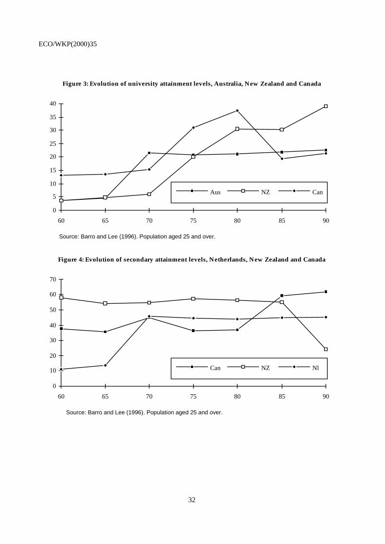
ECO/WKP(2000)35

32

Figure 3: Evolution of university attainment levels, Australia, New Zealand and Canada

0

5

10

15

20

25

30

35

40

60 65 70 75 80 85 90

Aus NZ Can

Source: Barro and Lee (1996). Population aged 25 and over.

Figure 4: Evolution of secondary attainment levels, Netherlands, New Zealand and Canada

0

10

20

30

40

50

60

70

60 65 70 75 80 85 90

Can NZ Nl

Source: Barro and Lee (1996). Population aged 25 and over.

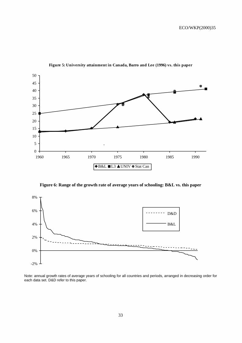
ECO/WKP(2000)35

33

Figure 5: University attainment in Canada, Barro and Lee (1996) vs. this paper

0

5

10

15

20

25

30

35

40

45

50

1960 1965 1970 1975 1980 1985 1990

B&L L3 UNIV Stat Can

Figure 6: Range of the growth rate of average years of schooling: B&L vs. this paper

-2%

0%

2%

4%

6%

8%

D&D

B&L

Note: annual growth rates of average years of schooling for all countries and periods, arranged in decreasing order foreach data set. D&D refer to this paper.

ECO/WKP(2000)35

34

Figure 7: Normalised average years of schooling: B&L vs. this paper

20

40

60

80

100

120

140

160

20 40 60 80 100 120 140 160

PorSp

It

Gr

Fr

Ost

Be

Nor

Dk

NZ

USCan

Ire

GerCH

Fin

Aus

SweUK

Jap

Nl

D&D normalized years of schooling

B&L normalized years of schooling -Note: Average number of years of schooling in each country (taken over all periods) are normalised by the unweightedsample average (=100). A regression of our normalised years of schooling on Barro and Lee’s gives the following result(t values in parentheses):Average years D&D = 35.43 + 0.646 avge.years B&L R2 = 0.683 (3.40) (6.40)

ECO/WKP(2000)35

35

Figure 8: Change in normalised average years of schooling between this paper and B&L

-30

-20

-10

0

10

20

30

Ost Fr Po CH Can Ger Nor Nl Jap It UK SpIr Gr Aus US

Sw Bel

NZFin

Dk

Figure 9: Estimated coefficient of human capital and 95% confidence interval around itwhen deleting one country at a time from the sample

-0,1

0

0,1

0,2

0,3

0,4

0,5

0,6

NZ Gr CH Ir Aus Sw Fi Nl Fr Be US Ost Dk It No Ge UK Sp Ca Po Ja

Note: Catch-up specification with country dummies (equation [6] in Table 9), estimated after excluding the country shown in thehorizontal axis.

ECO/WKP(2000)35

36

Figure 10: Average growth rates of productivity, per worker factor stocks and the TFP gapand investment rates in physical and human capital

-3%

-2%

-1%

0%

1%

2%

3%

4%

5%

6%

1960-65 1965-70 1970-75 1975-80 1980-85 1985-90

gq gk gh ggap

0,05

0,1

0,15

0,2

0,25

1960 1965 1970 1975 1980 1985 1990 1995

sk sh

Note: First panel: annualised growth rates of productivity (gq), the stock of capital per employed worker (gk), average years ofeducation (gh) and the TFP gap relative to the US. Second panel: sk is investment in physical capital as a fraction of GDP; sh istotal secondary and university enrolment as a fraction of the population over 15 (from World Development Indicators andUNESCO). All variables are average across countries in each sub-period.

ECO/WKP(2000)35

37

Figure 11: Relative productivity vs. relative TFP in 1960

Gr

Fin

Nor

Ire

Por

JapSp

UK

ItOst

Swe

AusGer

Fr

US

CHCan

Be

NZDk

Nl

relative productivity, 1960

relative TFP, 1960

-0.30 -0.20 -0.10 0.00 0.10 0.20 0.30

1

0

-1

tfprel60 = 0.353 qrel60 t = 6.67 R2 = 0.700

Figure 12: Relative productivity vs. relative TFP in 1990

Fin

Por

Gr

Nor

NZ

CH

Swe

Aus

DkJap

Ger

UK

Ost

Can

Ire Sp

NlFr

US

It

Bel

relative TFP, 1990

-0.20 -0.10 0.00 0.10 0.20 0.30

0.40

0.20

0.00

-0.20

-0.40

-0.60

relative productivity, 1990

tfprel90 = 0.472 qrel90 t = 4.41 R2 = 0.506

ECO/WKP(2000)35

38

Figure 13: Fraction of the productivity differential with the average explainedby the TFP gap in an average country in the sample

0,3

0,35

0,4

0,45

0,5

1960 1965 1970 1975 1980 1985 1990

ECO/WKP(2000)35

39

APPENDIX

1. Our revised attainment data are available at the following web site:http://iei.uv.es/~rdomenec/human.html.

1. Detailed country notes

United States

Source: U.S. Bureau of the Census (web site) for 1960, 1965, 1970, 1975, 1980, 1985, 1990 and 1995.

Population: 25+

Attainment categories: L1 = 4 years of schooling or less; L2.1 = 5-8 years; L2.2 = 9-12 years; L3.1 = 1-2years of college; L3.2 = more than two 2 years of college.

Netherlands

Source: Dutch Statistical Yearbooks with data for 1960, 1971 and 1990.

Population: labour force in 1960; population over 14 not attending school rest of the years.

Attainment categories (when not obvious how they correspond with our scheme): L2.1 = advancedelementary level (1960); L2.2 = secondary level (1960); L3.1 = semi-higher level (1960) and vocationalcolleges (1990).

Other notes: We use linear interpolation to fill in the missing observations.

Italy

Source: For secondary schooling, Italian Statistical Yearbooks with census data for 1961, 1981 and 1991,and DYB for 1970 (1971, 25+) . For university: UNESCO for 1960, DYB for 1971 and 1981 and EAG for1989. For illiterates, Statistical Yearbook for 1961, 1981 and 1991, and World Development Indicators for1970 and 1975.

Population: National yearbooks, 6+; UNESCO and DYB, 25+.

Other notes:

We do not use the information in the national yearbook for university attainment because this source refersto the population over 6 years of age and will therefore underestimate attainment (especially at this level).

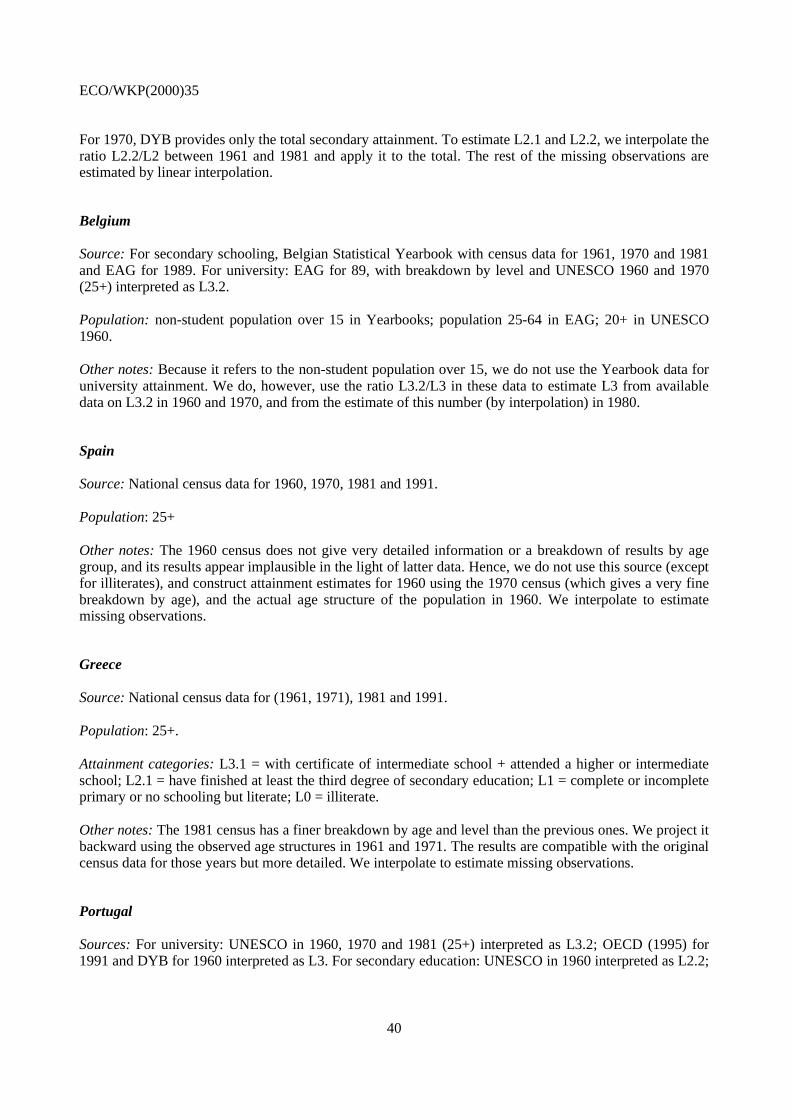
ECO/WKP(2000)35

40

For 1970, DYB provides only the total secondary attainment. To estimate L2.1 and L2.2, we interpolate theratio L2.2/L2 between 1961 and 1981 and apply it to the total. The rest of the missing observations areestimated by linear interpolation.

Belgium

Source: For secondary schooling, Belgian Statistical Yearbook with census data for 1961, 1970 and 1981and EAG for 1989. For university: EAG for 89, with breakdown by level and UNESCO 1960 and 1970(25+) interpreted as L3.2.

Population: non-student population over 15 in Yearbooks; population 25-64 in EAG; 20+ in UNESCO1960.

Other notes: Because it refers to the non-student population over 15, we do not use the Yearbook data foruniversity attainment. We do, however, use the ratio L3.2/L3 in these data to estimate L3 from availabledata on L3.2 in 1960 and 1970, and from the estimate of this number (by interpolation) in 1980.

Spain

Source: National census data for 1960, 1970, 1981 and 1991.

Population: 25+

Other notes: The 1960 census does not give very detailed information or a breakdown of results by agegroup, and its results appear implausible in the light of latter data. Hence, we do not use this source (exceptfor illiterates), and construct attainment estimates for 1960 using the 1970 census (which gives a very finebreakdown by age), and the actual age structure of the population in 1960. We interpolate to estimatemissing observations.

Greece

Source: National census data for (1961, 1971), 1981 and 1991.

Population: 25+.

Attainment categories: L3.1 = with certificate of intermediate school + attended a higher or intermediateschool; L2.1 = have finished at least the third degree of secondary education; L1 = complete or incompleteprimary or no schooling but literate; L0 = illiterate.

Other notes: The 1981 census has a finer breakdown by age and level than the previous ones. We project itbackward using the observed age structures in 1961 and 1971. The results are compatible with the originalcensus data for those years but more detailed. We interpolate to estimate missing observations.

Portugal

Sources: For university: UNESCO in 1960, 1970 and 1981 (25+) interpreted as L3.2; OECD (1995) for1991 and DYB for 1960 interpreted as L3. For secondary education: UNESCO in 1960 interpreted as L2.2;

ECO/WKP(2000)35

41

DYB in 1960 and UNESCO in 1970, 1981 and 1991 for L2. For illiterates (L0), World DevelopmentIndicators (WDI).

Population: 15+ in WDI, 25-64 in OECD (1995) and25+ in UNESCO and DYB.

Other notes:

University: We have observations for both L3.1 and L3.2 in 1960 and 1991. We calculate the ratio L3.2/L3in these two years and interpolate it to 1970 and 1981, where we have UNESCO observations that weinterpret as L3.2. Using the interpolated ratio and these observations, we estimate L3.1 and L3. Finally, weinterpolate for the rest of the years.

Secondary: We have an observation for L2.1 and L2.2 in 1960, and can obtain another one in 1991applying the ratio L2.2/L2 in OECD (1995) to the total L2 given in UNESCO (which refers to the desiredage group). We interpolate the ratio L2.2/L2 between 1960 and 1991 and apply it to available data on L2 toestimate its breakdown. We interpolate for the rest of the years.

France

Sources: National census for (1960), 1968, 1975 and 1990 and EAG (for 1989).

Population: 25+ not attending school in census data and pop. 25-64 in EAG.

Attainment categories in 1968. L2.1 = CEP, examen de fin d’apprentissage artisanal or certificat de fin destage de la FPA; L2.2 = BEPC, BE, BEPS, CAP, BEI, BEC, BES, BEH, BEA, etc; L3.1 = bac ou brevetsuperieur, brevet des ENP, brevet de technicien, etc., autres diplomes; L3.2 = superieur au bac complet.

Other notes: Data for 1960 are backward projections using 1968 attainments by age group and the 1960population structure. The 1990 Census seems to be missing secondary vocational qualifications, so we useEAG for 1989 instead at the secondary level.

Ireland

Sources: 1966 national census; UNESCO for 1981 and 1991. OECD (1995) for ratios L2.2/L2 andL3.2/L3.

Population: 25+ except OECD (1995) where it is 25-64.

Other notes:

Figures for 1961 are estimated by a backward projection of the 1966 census data on attainment by agegroup. Since we do not have the age structure of the population in 1961, we estimate it from the 1966distribution using age-specific survival probabilities (for 1981) taken from the DYB. To compute theaverage survival probability, we assume 40 per cent of population is urban in 1961 (around 55 per cent in1981) to average death rates over rural and urban populations.

Census and survey information does not allow a breakdown of L3 and L2 into first and second cycles. Weestimate this breakdown using data from OECD (1995). For L2 we have L2.1 and L2.2 in 1991 fromUNESCO. OECD (1995) gives this ratio by age group; we observe that the ratio L2.1/L2.2 stabilises forthe older age groups around 0.54, which we take as the 1960 value, then we interpolate this ratio between

ECO/WKP(2000)35

42

the two observations and apply the result to our L2 series to recover L2.1 and then L2.2. To recover L3.1and L3.2 we proceed in a similar way, we use the ratio L3.1/L3 in OECD 1995. Since this ratio does notchange much with age in this source, we keep its value constant over time.

The remaining missing observations are filled in by interpolation. The figures for 1960 are extrapolationsfrom 1960 and 1966 estimates.

Sweden

Sources: National Statistical Yearbook for 1970 and 1994, Education in Nordic Countries for ratio L3.1/L3en 1988.

Population: 25+ (est.) in 1970 and 25-75 in 1994.

Other notes:

The earliest available disaggregated data is for 1970 and refers to the population aged 25-60. We want touse this information (and census data on the age structure of the population) to estimate attainment in thesame year and in 1960 for the population 25+. First, we extrapolate attainment rates to older cohorts in1970 as follows. Let F3544 and F4559 be the fraction of the population aged 35-44 and 45-59 that hasattained a given level of education. Then, we estimate F6075 and F75+ as follows:

F6075 = F4559 + 0.5* (F4559 - F3544)

F75+ = F4559 + (F4559 - F3544).

With this, we can estimate attainments for ages 25+ in 1970, using the age structure of the population inthat year. Next, we estimate 1960 using the same information and the age structure in 1960.

Breakdown for tertiary into L3.1 and L3.2: We have data on the two cycles and therefore on the ratioL3.1/L3 for 1960, 1970 and 1994 from the Statistical Yearbook and for 1988 from Education in NorthernCountries. For the rest of the years we interpolate this ratio and total L3, and use these two numbers toestimate L3.1 and L3.2.

Norway

Source: Statistics Norway web site for 1960, 1970, 1975, 1980, 1985 and 1990.

Population: 16+

Other notes:

Statistics Norway does not disaggregate compulsory education into L1 and L2.1 or tertiary achievementinto L3.1 and L3.2. We use information from Sweden and Education in Nordic Countries (1994) toestimate these categories as follows.

To estimate L3.1 and L3.2: We have data on these two categories in 1988 for all Scandinavian countriesfrom Education in Nordic Countries. We compute the quotient L3.1/L3 for Norway and Sweden and theratio between them. We then apply this ratio to the Swedish L3.1/L3 ratio to estimate the Norwegian ratiofor all years and use it to recover L3.1 and L3.2.

ECO/WKP(2000)35

43

To estimate L1 and L2.1,we use the ratio L1/L1+L2.1 for Sweden.

Denmark

Sources: Danish Statistical Yearbooks with data for 1983, 1988 and 1991 and OECD (1974) for attainmentgrowth rates between 1960 and 1971.

Population: 25-62 or 25-65.

Other notes:

National sources and OECD report only L1+L2.1 (compulsory education). To separate them we use theratio L1/L1+L2.1 for Sweden.

Figures for 1973 are a backward projection using attainment data by age in 1983 and the age structure ofthe population in 1971. We then extrapolate back to 1970 using the 1973 and 1983 observations. Finally,we use the annual growth rate of attainment between 1960 and 1971 reported in OECD (1974) to estimate1960 levels of L3 and L2 (We use the growth rate of attainments, which is recovered from the original dataon average years of schooling by level. It coincides with the original for L3 but not for L2 since peoplewith university schooling also have secondary training and we have to subtract them from the total to getthose whose maximum attainment level is secondary). L2.1 in 1960 is obtained from the 1970 value andthe growth rate for secondary, for all other years we use the Swedish ratio L2.1/L1+L2.1.

Backward projection for 1973: The 1983 disaggregation by age stops with the group 60-62. We estimateattainments for the 63-64 population by extrapolating the change between the previous two age groups andweighting it for the “length of the period”, and reconstruct attainment for the 60-64 age group. Then weextrapolate backwards again from consecutive age groups of the same length but assuming that at each stepthe change in the achievement ratios drops to one half for each category (This is half way betweenextrapolating and attributing to the oldest group in the population the achievement of the last observed agesubgroup).

1988 Statistical Yearbook secondary attainment figures look implausible and are ignored.

Tertiary is broken down into three groups: post-secondary vocational (isced5), short university courses andfull-length university degrees. We report the sum of the first two groups as L3.1.

Finland

Sources: For university, UNESCO in 1960, 1970, 1980, 1985 and 1990 (all for L3); Education in NordicCountries for ratio L3.2/L3 in 1988. For secondary, in 1960 DYB for L2 and UNESCO interpreted asL2.1, in 1970 UNESCO interpreted as L2.2, in 1980 UNESCO gives breakdown of L2 into L2.1 and L2.2,in 1990 UNESCO interpreted as L2.2.

Population: 20+ in 1980, and 25+ in 1990. We need to check the rest.

Other notes:

Most sources do not separate L3.1 and L3.2. Those that do (towards the end of the period) give extremelysimilar values. We take the 1988 ratio from Education in Nordic Countries and assume that it remainsconstant throughout the whole sample period. We use this ratio to recover L3.1 and L3.2.

ECO/WKP(2000)35

44

Secondary: we interpolate and extrapolate L2 to recover missing observations and the ratio L2.2/L2 toseparate the first and second cycle.

Japan

Sources: For higher education, DYB for 1960 (25+) and 1970 (25+), UNESCO for 1980 and 1990,UNESCO for 1970 interpreted as L3.2, and EAG for ratio L3.1/L3 in 1990. For secondary attainment, in1960 and 1965 UNESCO interpreted as L2.2. For 1960 and 1970 we recover an estimate of L2 from thedata on average years of secondary schooling in OECD (1974). In 1990, UNESCO, interpreted as L2.2.

Population: UNESCO and DYB, 25+; EAG, 25-64.

Other notes:

Tertiary attainment: In 1990, we use ratio L3.1/L3.2 from EAG for 1989 to estimate L3.1 and L3.2. Weinterpolate and extrapolate the ratio L3.1/L3.2 from available years (1970 and 1990) to estimate L3.1 andL3.2 in the rest of the period.

Secondary attainment: We interpolate L2.2 between available observations to recover the complete series.Then, we compute the ratio L2.1/L2.2 for 1960 and 1970 and extrapolate it forward to 1980 and 1990(assuming the increase between each two decades drops to one half its previous value at each stage). Weuse this ratio to estimate L2.1 and add it to L2.2 to obtain L.2. Remaining missing observations are filledby interpolation.

New Zealand

Sources: Higher education: Statistical Yearbook for 1965 and 1970, interpreted as L3.2 and for 1975 and1981, interpreted as L3; OECD (1995) for 1992 with full breakdown. Secondary schooling: StatisticalYearbook for 1965; for 1981 we use the DYB and add to this source’s reported L2.2 part of Barro andLee’s L3, as explained below. For 1992 we use OECD (1995), adding to L2.2 part of Barro and Lee’sL3.1, as above.

Population: 25+ except OECD (1995).

Other notes:

Higher education: We interpolate L3.2 between 1970 and 1992, compute the ratio L3.2/L3 for 1975onwards and extrapolate this ratio back to recover L3 and its breakdown in 1965 and 1970. Finally, weextrapolate backward L3 and the ratio L3.2/L3 to estimate attainments in 1960. We assume the differencebetween Barro and Lee’s L3 and our estimate is part of L2.2 and add it to that category.

Secondary education: For L2, we interpolate between 1965, 1981 and 1991, and extrapolate backward to1960. We compute the ratio L2.2/L2 in 1981 and 1991 and interpolate it between these years. We assumethis ratio remains constant for all years before 1981 and use it to break down L2 into its upper and lowerlevels.

ECO/WKP(2000)35

45

United Kingdom

Sources: For higher education, in 1960 UNESCO interpreted as L3.2; in 1975 (1976), UNESCO for L3; in1991 EAG93 for L3.1 and L3.2. For secondary attainment: UNESCO for 1960 and 1970 interpreted asL2.2, EAG93 gives L2.2 for 1991.

Population: UNESCO 1976, 25-69. EAG, 25-64. UNESCO 25+.

Other notes:

Higher education: We interpolate L3.2 between 1960 and 1991 to recover the full series. Then, wecompute the ratio L3.2/L3 in 1975 and 1991, interpolate it between these years and extrapolate it backwardto 1960. Using this ratio, we estimate L3.1 and L3 in 1960. Then we interpolate between these years.

Secondary education: We interpolate between available observations to complete the L2.2 series. Toconstruct L2.1, we use a regression estimate of the ratio L2.1/L2.2 (see the body of the paper).

Double check UNESCO 1970.

Switzerland

Sources: Higher education: for 1960, UNESCO as L3; for 1970, UNESCO interpreted as L3.2; for 1991,EAG for L3.1 and L3.2. For secondary education: In 1960, UNESCO interpreted as L2.2; in 1980, Kaneko(as reported in Barro and Lee’s appendix) interpreted as L2.2; and in 1991, EAG for L2.2.

Population: 25+

Other notes:

Higher education: We interpolate L3 and L3.2 between available observations, compute the ratio L3.2/L3,extrapolate it back to 1960 and use it to estimate L3.1 and L3.2 in that year. In all years, L3.1 is computedas the difference between the estimated values of L3 and L3.2.

Secondary education: We interpolate between available observations to recover the L2.2 series. We use aregression estimate of the ratio L2.1/L2.2 to estimate L2.1.

Austria

Sources: University, UNESCO for 1961, 1971, 1981 and 1991 interpreted as L3.2 and 1995 Microcensusfor L3.1 and L3.2. Secondary, L2.2 from the Austrian Statistical Yearbook for 1961, 1971, 1981 and 1991and the 1995 Microcensus.

Population: UNESCO, 25+; microcensus, check; Austrian Statistical Yearbook, 16+.

Other notes:

University: We use the ratio L3.1/L3.2 from the 1995 microcensus (which does not vary significantlyacross age groups) to estimate L3.1 in years before 1995. Our guess for L3.1 in the 1995 microcensus iscalled “secondary technical and vocational” and lasts 5 years, two more than other upper secondary

ECO/WKP(2000)35

46

categories. We don’t use the Austrian Statistical Yearbook series for university schooling because it refersto the population 16+ and will tend to underestimate tertiary attainment.

Secondary: For 1961-91, we guess that reported L2.2 includes our estimate of L3.1, so we subtract it fromreported L2.2 to obtain the final estimate. For L2.2, we interpolate between available observations andextrapolate backward from 1961 to 1960. To estimate L2.1, we use a regression estimate of the ratioL2.1/L2.2.

Australia

Sources: University, in 1965 UNESCO (as reported in Barro and Lee) interpreted as L3.2; in 1970 (1971)UNESCO (as reported in Barro and Lee) as L3, and in 1990, EAG for L3.1 and L3.2. Secondary: For 1965we use as L2 UNESCO minus our estimate of L3.1; for 1970 UNESCO as L2, for 1990, we have L2.1 andL2.2 from EAG.

Population: 25+

Other notes:

University: We interpolate between 1965 and 1990 to estimate L3.2, and between 1970 and 1990 toestimate L3.1. Then, we compute the ratio L3.2/L3 and extrapolate it backward to 1965 and 1960. We usethe estimated ratio to recover L3 (and hence L3.1) in 1965. For 1960, first we extrapolate L3.2 backwardand then proceed in the same way.

Secondary: We interpolate L2 for missing years after 1965 and use the ratio L2.2/L2 from EAG in 1990(assumed constant over time) to recover L2.1 and L2.2. For 1960, we first extrapolate L2 backwards andthen use the same ratio.

EAG gives the same figures for 1989 and 1993, so we use the same number for 1990 without“periodification”.

Germany

Sources: University: EAG for 1991; in 1970 DYB interpreted as L3; in1970 UNESCO, 1975 and 1980 (infact 1978 and 1982) Statistiches Jahrbuch as reported in Barro and Lee, all interpreted as L3.2. From 1970backward we use the growth rate of attainment recovered from OECD (1974). Secondary: OECD (1974)for 1960 and 1970 as L2; for 1970 and 1980 DYB interpreted as L2.2 and for 1991 EAG gives L2.2 andL2.1.

Population: UNESCO and DYB, 25+; EAG, 25-64.

Other notes:

University: We interpolate between available observations for 1970 on. To extrapolate backward from1970 we use the growth rate of university attainment given in OECD (1974).

Secondary schooling: We use the ratio L2.1/L2 from 1970 to estimate L2.1 in other years, given L2. In1991 this gives a number for L2+L3 slightly larger than 100, so we accept the L2.1 ratio for that year givenby EAG, and the implication that L1 is zero.

ECO/WKP(2000)35

47

Canada

Sources: Higher education: We interpret UNESCO’s 1960, 1986 and 1991 observations, and the DYBobservation for 1975 as referring to university attainment in the narrow sense [i.e. UNIV = L3 - L3.1(5)].We interpret the 1960 DYB figure as referring to L3.2. We interpret UNESCO for 1976 and 1981 andOECD (1995) for 1992 as L3. We use National Census figures for the ratio L3.1(6)/L3.2 in 1986 and 1991.Secondary schooling: UNESCO for 1960 interpreted as L2.2; Statistics Canada web site for L2.2 in 1976,1981, 1986 and 1991.

Population: National Census, 15+; UNESCO and DYB, 25+; OECD, 25-64.

Other notes:

University: see the discussion in the text.

Secondary: For L2.2, we fill in missing observations by interpolation. No data are reported for L2.1, whichseems to be grouped together with L2.1 as a single category. We estimate L2.1 by using de L1/(L1+L2.1)ratio for the United States.

2. Data tables

2. Tables A1-A3 contain our estimates of attainment levels (in percentages) for the adult population.We report higher and secondary attainment for all countries in the sample, and an illiteracy series for fourcountries (Spain, Italy, Greece and Portugal). For the remaining countries, illiteracy rates are extremelylow and are therefore ignored. Primary attainment can be obtained as L1 = 100 - L3 - L2 (- L0). Charactertypes are used to indicate data quality as indicated in the note to Table A.1.

3. Table A4 contains an estimate of the average number of years of total schooling. This isconstructed by combining the attainment series with the cumulative duration by educational level andcountry given in Table 6 in the text.

4. Tables A5-A7 give the data sources and summarise the estimation method used to obtain eachobservation. See the notes to Table A5 for a key to the notation used in these tables. Notice thatinterpolations are generally constructed taking into account the exact year to which the original observationrefers, rather than bringing them to the beginning or the end of the quinquenium.

5. Figures A1-A4 plot our attainment and years of schooling series together with Barro and Lee’s tofacilitate country-by-country comparisons between the two data sets.

3. Estimation of the stock of physical capital

6. We construct series of stocks of physical capital in the OECD countries for the period 1950-97using a perpetual inventory procedure with an assumed annual depreciation rate of 5 per cent. To estimatethe initial capital stock we modify the procedure proposed by Griliches (1980) to take into account the factthat the economies in our sample may be away from their steady states.

7. The growth rate of the stock of capital, gk, can be written in the form:

δ−= ��

��

ECO/WKP(2000)35

48

where I is investment, δ the depreciation rate and K the stock of capital. Solving this expression for K andassuming that the growth rate of investment is a good approximation to the growth rate of the capital stock(i.e. gI ≅ gk), we obtain an expression that can be used to estimate the initial capital stock using data oninvestment flows:

K = δ+

N�� ≅

δ+,

�� . [A.1]

When implementing this approach, it is common to use the level of investment in the first year in thesample period and the growth rate of the same variable over the entire period. In our case, however, thisdoes not seem to be the best way to proceed because i) investment may be subject to transitorydisturbances that make it dangerous to rely on a single observation and ii) rates of investment and factoraccumulation will tend to vary over time in a systematic way as countries approach their steady states.

8. To try to control for these factors, we use the growth rate of investment over the period 1950-60and the HP-filtered level of investment in 1955. Hence, our version of equation [A.1] is of the form:

K55 ≅��

��

��+−�

,

KS� , [A.2]

where Ihp is the Hodrick-Prescott trend of investment (with a smoothing parameter λ = 10). We use 1955as the base year instead of 1950 because it is known that this filter may displays anomalies at sampleendpoints.25 Our investment data are corrected for differences in PPP and are taken from the OECDNational Accounts and Economic Outlook starting in 1960. Prior to that date, we use IMF data and pricedeflators and, for some countries where no information is available, we extrapolate investment backwardusing the growth rates of the capital stocks provided by Summers and Heston in the PWT 5.6.

25. Due to data limitations and other anomalies we have used a different base year for some countries. In

particular, we use 1953 for Canada and Norway and 1960 for the UK, Greece and Ireland.

ECO/WKP(2000)35

49

Table A1: University attainment levels

Country level 1960 1965 1970 1975 1980 1985 1990 1995United States L3 16.50 18.30 21.20 26.30 31.90 35.70 39.20 47.80United States L3.1 8.80 8.90 10.20 12.40 14.90 16.30 17.90 24.80United States L3.2 7.70 9.40 11.00 13.90 17.00 19.40 21.30 23.00

Netherlands L3 3.30 4.64 5.97 8.22 10.70 13.18 15.66Netherlands L3.1 1.90 3.11 4.32 5.92 7.62 9.32 11.02Netherlands L3.2 1.40 1.53 1.65 2.30 3.08 3.86 4.64

Italy L3.2 = L3 2.10 2.81 3.51 4.19 4.87 5.50 6.13

Belgium L3 8.27 9.19 10.10 13.13 16.16 18.30 20.43Belgium L3.1 4.27 4.44 4.60 6.45 8.30 9.24 10.19Belgium L3.2 4.00 4.75 5.50 6.68 7.87 9.05 10.24

Spain L3 3.07 3.53 3.98 5.41 6.84 8.17 9.48Spain L3.1 1.59 1.85 2.11 2.77 3.43 4.08 4.73Spain L3.2 1.48 1.68 1.87 2.64 3.42 4.09 4.75

Greece L3 3.71 4.31 4.92 6.56 8.45 9.73 10.86Greece L3.1 1.13 1.31 1.49 2.43 3.56 3.41 2.93Greece L3.2 2.58 3.00 3.43 4.12 4.89 6.33 7.94

Portugal L3 1.50 1.70 1.90 3.18 4.46 5.51 6.50Portugal L3.1 0.40 0.45 0.50 0.82 1.15 1.41 1.65Portugal L3.2 1.10 1.25 1.40 2.35 3.31 4.10 4.85

France L3 9.41 10.43 11.79 13.68 16.43 19.17 21.92France L3.1 6.83 7.54 8.32 9.19 11.48 13.76 16.05France L3.2 2.58 2.89 3.48 4.49 4.95 5.41 5.87

Ireland L3 4.03 4.36 5.36 6.51 7.67 10.58 13.93Ireland L3.1 2.05 2.22 2.73 3.31 3.90 5.38 7.09Ireland L3.2 1.98 2.14 2.63 3.20 3.77 5.20 6.84

Sweden L3 4.83 5.74 6.65 9.71 12.77 15.83 18.89 21.34Sweden L3.1 2.10 2.41 2.71 4.27 5.83 7.39 8.95 10.20Sweden L3.2 2.73 3.34 3.94 5.44 6.94 8.44 9.94 11.14

Norway L3 4.20 5.45 6.70 8.70 11.10 13.60 15.70Norway L3.1 2.00 2.50 3.00 3.99 5.22 6.56 7.86Norway L3.2 2.20 2.95 3.70 4.71 5.88 7.04 7.84

Denmark L3 7.08 9.93 12.79 14.79 16.78 18.26 19.31Denmark L3.1 5.26 7.39 9.52 11.19 12.87 14.01 14.61Denmark L3.2 1.81 2.55 3.28 3.60 3.92 4.25 4.70

Finland L3 4.10 5.10 6.10 9.00 11.90 13.80 15.40Finland L3.1 1.84 2.29 2.74 4.04 5.34 6.20 6.92Finland L3.2 2.26 2.81 3.36 4.96 6.56 7.60 8.48

Japan L3 6.30 7.87 9.43 11.87 14.30 17.75 21.20Japan L3.1 2.63 3.28 3.93 4.82 5.70 6.89 8.08Japan L3.2 3.67 4.59 5.50 7.05 8.60 10.86 13.12

ECO/WKP(2000)35

50

Table A1: University attainment levels (continued)______________________________________________________________________________________Country level 1960 1965 1970 1975 1980 1985 1990 1995New Zealand L3 11,96 14,08 16,20 18,90 21,44 22,55 23,30New Zealand L3.1 7.86 9.11 10.31 11.83 13.19 13.14 12.69New Zealand L3.2 4.09 4.97 5.89 7.07 8.25 9.41 10.61

United Kingdom L3 3.88 6.25 8.63 11.00 12.88 14.75 16.63United Kingdom L3.1 2.08 3.13 4.18 5.23 5.78 6.34 6.89United Kingdom L3.2 1.80 3.12 4.45 5.77 7.09 8.41 9.74

Switzerland L3 9.40 11.11 12.82 14.53 16.24 17.95 19.66Switzerland L3.1 7.96 8.94 9.92 10.65 11.39 12.12 12.85Switzerland L3.2 1.44 2.17 2.90 3.88 4.85 5.83 6.80

Austria L3 4.12 4.50 4.88 6.03 7.36 9.23 11.24 12.40Austria L3.1 1.96 2.14 2.32 2.87 3.50 4.39 5.35 5.90Austria L3.2 2.16 2.36 2.56 3.16 3.86 4.84 5.89 6.50

Australia L3 15.66 18.79 21.50 23.88 26.25 28.63 31.00Australia L3.1 12.02 14.09 15.74 17.06 18.37 19.69 21.00Australia L3.2 3.64 4.70 5.76 6.82 7.88 8.94 10.00

Germany L3 6.64 7.57 8.50 12.21 14.93 18.14 21.36Germany L3.1 4.22 4.81 5.40 6.71 8.03 9.38 10.73Germany L3.2 2.42 2.76 3.10 5.50 6.90 8.76 10.63

Canada L3 25.03 26.88 28.73 30.75 36.15 38.75 40.43Canada L3.1(5) 11.93 12.82 13.70 14.66 18.65 19.75 19.45Canada L3.1(6) 6.60 6.87 7.14 7.49 8.20 9.01 9.81Canada L3.2 6.50 7.20 7.90 8.60 9.30 9.99 11.17Canada UNIV 13.10 14.07 15.03 16.00 17.50 19.00 20.98______________________________________________________________________________________

Note: Character types are used to indicate the quality of the data. A bold character indicates a direct census orsurvey observation (or interpolation from census or survey data no more than two years away in time). Bolditalic indicates that we are using census or survey data (usually from UNESCO or DYB compilations) afterreinterpreting it as an attainment category slightly different from the one reported in the original source. Italicsare used for educated guesses based on census or survey information (e.g. when we apply ratios from acensus source to census totals to break down an attainment category into subcategories). The rest of theobservations are interpolations or more uncertain estimates.

ECO/WKP(2000)35

51

Table A2: Secondary attainment levels______________________________________________________________________________________Country Level 1960 1965 1970 1975 1980 1985 1990 1995United States L.2 75.20 74.90 73.50 69.50 64.80 61.60 58.40United States L2.1 31.40 26.20 22.40 17.70 14.10 11.20 8.80United States L2.2 43.80 48.70 51.10 51.80 50.70 50.40 49.60

Netherlands L.2 40.60 46.00 51.39 55.18 58.57 61.96 65.35Netherlands L2.1 33.50 37.81 42.13 40.12 36.52 32.93 29.34Netherlands L2.2 7.10 8.18 9.26 15.07 22.05 29.03 36.01

Italy L2 12.73 18.30 23.87 29.06 34.25 40.88 47.87Italy L2.1 8.82 12.59 16.34 19.74 23.13 26.56 30.00Italy L2.2 3.91 5.71 7.53 9.32 11.12 14.32 17.87

Belgium L2 27.55 31.05 34.55 40.07 45.59 48.345 50.414Belgium L2.1 22.14 23.14 24.13 25.99 27.85 29.11 30.223Belgium L2.2 5.41 7.91 10.41 14.07 17.74 19.235 20.191

Spain L2 4.20 5.03 5.85 9.21 12.57 19.74 27.86Spain L2.1 2.17 2.71 3.24 5.21 7.18 10.95 15.17Spain L2.2 2.03 2.32 2.61 4.00 5.39 8.79 12.69

Greece L2 12.53 13.75 14.97 16.89 19.00 22.30 25.89Greece L2.1 4.31 4.58 4.86 5.34 5.87 6.10 6.24Greece L2.2 8.22 9.17 10.11 11.56 13.13 16.20 19.65

Portugal L2 6.40 6.60 6.80 8.53 10.25 12.28 14.38Portugal L2.1 2.90 3.07 3.24 4.19 5.13 6.30 7.53Portugal L2.2 3.50 3.53 3.56 4.34 5.12 5.98 6.85

France L2 47.45 53.99 59.28 62.70 61.38 60.06 58.74France L2.1 36.18 40.31 41.40 37.95 33.68 29.41 25.15France L2.2 11.27 13.69 17.89 24.75 27.70 30.64 33.59

Ireland L2 23.21 26.00 30.09 34.50 38.92 42.36 45.56Ireland L2.1 12.55 13.50 14.86 16.32 17.79 18.49 19.00Ireland L2.2 10.66 12.50 15.23 18.18 21.13 23.87 26.56

Sweden L2 30.22 33.80 37.38 40.68 43.97 47.27 50.56 53.20Sweden L2.1 7.25 8.39 9.53 9.84 10.14 10.45 10.76 11.00Sweden L2.2 22.97 25.41 27.85 30.84 33.83 36.82 39.81 42.20

Norway L2 24.28 29.14 34.00 38.86 44.06 49.99 53.23Norway L2.1 7.98 9.04 10.10 11.36 11.96 11.69 11.83Norway L2.2 16.30 20.10 23.90 27.50 32.10 38.30 41.40

Denmark L2 38.73 40.83 42.93 46.41 49.64 51.83 52.44Denmark L2.1 6.05 6.79 7.54 8.29 8.79 9.56 10.70Denmark L2.2 32.68 34.04 35.40 38.12 40.85 42.27 41.75______________________________________________________________________________________

ECO/WKP(2000)35

52

Table A2: Secondary attainment levels (continued)______________________________________________________________________________________Country Level 1960 1965 1970 1975 1980 1985 1990 1995Finland L2 27.80 29.13 30.47 33.68 36.90 40.59 44.28Finland L2.1 6.00 6.23 6.47 7.08 7.70 8.39 9.08Finland L2.2 21.80 22.90 24.00 26.60 29.20 32.20 35.20

Japan L2 38.70 43.43 48.30 52.54 56.77 60.87 64.96Japan L2.1 7.80 10.43 13.07 15.07 17.07 18.77 20.46Japan L2.2 30.90 33.00 35.23 37.47 39.70 42.10 44.50

New Zealand L2 53.82 54.80 55.78 56.77 57.75 58.70 59.63New Zealand L2.1 21.11 21.49 21.88 22.27 22.65 18.71 13.52New Zealand L2.2 32.71 33.31 33.90 34.50 35.10 39.99 46.11

United Kingdom L2 39.38 43.58 47.24 53.18 58.05 62.26 65.57United Kingdom L2.1 14.88 16.88 18.34 19.49 19.58 19 17.53United Kingdom L2.2 24.50 26.70 28.90 33.69 38.47 43.26 48.04

Switzerland L2 41.68 47.77 53.27 58.16 62.38 67.94 72.15Switzerland L2.1 19.88 20.79 21.12 20.83 19.88 17.49 13.74Switzerland L2.2 21.80 26.98 32.15 37.33 42.50 50.45 58.41

Austria L2 47.9 49.65 50.05 53.8 57.99 61.58 64.63Austria L2.1 16.14 17.08 16.67 17.24 17.66 17.82 17.53Austria L2.2 31.76 32.57 33.38 36.56 40.33 43.76 47.10 51.5

Australia L2 37.92 43.11 48.30 49.98 51.65 53.33 55.00Australia L2.1 20.69 23.52 26.35 27.26 28.17 29.09 30.00Australia L2.2 17.24 19.60 21.95 22.72 23.48 24.24 25.00

Germany L2 53.60 55.70 57.80 64.75 71.70 74.57 77.43Germany L2.1 14.28 14.84 15.40 17.25 19.10 18.60 18.10Germany L2.2 39.32 40.86 42.40 47.50 52.60 55.96 59.33

Canada L2 67.22 66.26 65.62 64.35 60.03 57.66 55.93Canada L2.1 29.32 26.44 23.88 20.68 16.30 14.89 13.36Canada L2.2 37.90 39.82 41.74 43.67 43.73 42.77 42.57______________________________________________________________________________________

ECO/WKP(2000)35

53

Table A.3: Illiteracy rates______________________________________________________________________________________Country Level 1960 1965 1970 1975 1980 1985 1990Italy L0 8.58 7.29 6.00 5.10 3.41 2.698 2.23Spain L0 11.20 10.63 10.05 9.48 8.90 7.01 4.79Greece L0 23.92 20.81 17.69 14.78 11.92 10.35 9.09Portugal L0 34.00 30.20 26.40 22.60 18.30 15.70 12.80______________________________________________________________________________________

Table A.4: Average years of schooling_______________________________________________________________________________

1960 1965 1970 1975 1980 1985 1990Australia 10.15 10.67 11.15 11.43 11.71 12.00 12.28Austria 9.12 9.24 9.33 9.68 10.09 10.53 10.95Belgium 7.55 7.81 8.07 8.61 9.16 9.47 9.76Canada 11.54 11.74 11.96 12.16 12.54 12.69 12.80Denmark 9.09 9.46 9.83 10.21 10.58 10.84 10.93Finland 7.88 8.05 8.22 8.68 9.13 9.50 9.87France 8.13 8.57 9.04 9.57 9.86 10.16 10.45Germany 9.17 9.46 9.74 10.76 11.66 12.32 12.99Greece 5.56 5.87 6.18 6.62 7.09 7.51 7.91Ireland 7.38 7.55 7.84 8.17 8.49 8.94 9.41Italy 5.42 5.83 6.25 6.63 7.05 7.52 8.01Japan 8.67 9.01 9.37 9.79 10.21 10.73 11.24Netherlands 8.11 8.48 8.85 9.35 9.88 10.42 10.95Norway 7.60 7.97 8.35 8.78 9.29 9.88 10.25New Zealand 10.46 10.72 10.98 11.30 11.60 11.86 12.11Portugal 4.37 4.62 4.87 5.29 5.73 6.06 6.41Spain 4.97 5.08 5.19 5.53 5.87 6.45 7.10Sweden 8.04 8.30 8.57 9.03 9.49 9.96 10.42Switzerland 9.08 9.64 10.20 10.73 11.24 11.91 12.53United States 11.44 11.69 11.93 12.24 12.53 12.74 12.91United Kingdom 8.26 8.67 9.06 9.60 10.07 10.51 10.94

_______________________________________________________________________________

ECO/WKP(2000)35

54

Table A.5: Data sources and construction, university attainment

Country level 1960 1961 1965 1966 1968 1970 1971 1975 1980 1981 1985 1989 1990 1991 1995United States L3.1 NC NC NC NC NC NC NC NC

United States L3.2 NC NC NC NC NC NC NC NC

Netherlands L3.1 NC int int NC int int int NC


Italy L3.2 UNE int DYB int DYB int EAG ext

Belgium L3 est int est (NC) int est (NC) int EAG ext

Belgium L3.1 est int est (NC) int est (NC) int EAG ext

Belgium L3.2 UNE int DYB int int int EAG ext

Spain L3.1 BP int NC int int NC int int NC


Greece L3.1 ext BP int int BP int int NC int int NC


Portugal L3 DYB int est int est int int OECD95

Portugal L3.1 est int est int est int int OECD95

Portugal L3.2 UNE int UNE int int UNE int int OECD95

France L3 BP int NC int NC int int NC

France L3.1 BP int NC int NC int int NC

France L3.2 BP int NC int NC int int NC

Ireland L3 ext BP int NC int int int UNE int int UNE

Ireland L3.1 ext Est int est int int int est int int est(OECD95)

Ireland L3.2 ext Est int est int int int est int int est(OECD95)

ECO/WKP(2000)35

55

Table A.5: Data sources and construction, university attainment (continued)

Country level 1960 1965 1970 1973 1975 1980 1981 1983 1985 1988 1990 1991 1992 1994Sweden L3 BP int NC int int int int NC

Sweden L3.1 BP est NC est est est est NC

Sweden L3.2 BP est NC est est est est NC

Norway L3 NC int NC NC NC NC NC

Norway L3.1 Est int est est est est est (EdNC)

Norway L3.2 Est int est est est est est (EdNC)

Denmark L3 est(OECD74)

int ext BP int int NC int NC int NC

Denmark L3.1 Est int ext BP int int NC int NC int NC

Denmark L3.2 Est int ext BP int int NC int NC int NC

Finland L3 UNE int UNE int UNE UNE UNE

Finland L3.1 Est int est int est est Ed in NC

Finland L3.2 Est int est int est est Ed in NC

Japan L3 DYB int DYB int UNE int UNE

Japan L3.1 Est int est int est int EAG89

Japan L3.2 Est int UNE int est int EAG89

New Zealand L3 Ext ext ext NC int NC int int OECD95

New Zealand L3.1 Est est est est est est est est OECD95

New Zealand L3.2 Est NC NC int int int int int OECD95

United Kingdom L3 est int int UNE int int int EAG91

United Kingdom L3.1 est int int est int int int EAG91

United Kingdom L3.2 UNE int int int int int int EAG91

ECO/WKP(2000)35

56

Table A.5: Data sources and construction, university attainment (continued)

Country Level 1960 1961 1965 1970 1971 1975 1976 1980 1981 1985 1986 1990 1991 1992 1995Switzerland L3 UNE int Int int int int int EAG91

Switzerland L3.1 est est Est est est est est EAG91

Switzerland L3.2 est est UNE int int int int EAG91

Austria L3 ext Est int Int est int int est int int est NC

Austria L3.1 ext Est int Int est int int est int int est NC

Austria L3.2 ext UNE int Int UNE int int UNE int int UNE NC

Australia L3 est est UNE int int int EAG

Australia L3.1 est est Est est est est EAG

Australia L3.2 ext UNE Int int int int EAG

Germany L3 est(OECD74)

est DYB int int int int EAG91

Germany L3.1 est est Est est est est est EAG91

Germany L3.2 est est UNE SJ SJ int int EAG91

Canada L3 est est Est est UNE int UNE int int int int OECD95

Canada L3.1(5) est est Est est est int int est int est

Canada UNIV* UNE int Int int DYB int int UNE int UNE

Canada L3.1(6) est est Est est est int int est int est

Canada L3.2 DYB int Int int int int int NC int NC

(*) UNIV = university attainment, excluding upper level vocational training (ISCED 5) = L3.1(6) + L3.1.

Key: NC = national census or survey data, or national statistical yearbook; DYB = UN Demographic Yearbook; UNE = UNESCO Yearbook; EAG = OECD,Education at a Glance; OECD95 = OECD (1995); B&L = Barro and Lee (1996); EdinNC = Educational indicators in the Nordic countries (1974); SJ =Statistiches Jahrbuch, as reported in Barro and Lee. int = interpolation between available observations; ext = extrapolation (forward or backward); est =indirect estimate; BP = Backward projection using census or survey data disaggregated by age.

ECO/WKP(2000)35

57

Table A.6: Data sources and construction, secondary attainment

Country Level 1960 1961 1965 1966 1968 1970 1971 1975 1980 1981 1985 1989 1990 1991 1995United States L2.1 NC NC NC NC NC NC NC NC

United States L2.2 NC NC NC NC NC NC NC NC



Italy L2 ext NC int DYB int int int NC int int NC

Italy L2.1 ext NC int est int int int NC int int NC

Italy L2.2 ext NC int est int int int NC int int NC

Belgium L2.1 ext NC int NC int int int NC int EAG ext

Belgium L2.2 ext NC int NC int int int NC int EAG ext





Portugal L2 DYB int UNE int UNE int int UNE

Portugal L2.1 est int est int est int int est(OECD)

Portugal L2.2 UNE int est int int est int int est(OECD)

France L2 BP int NC int NC int int EAG ext

France L2.1 BP int NC int NC int int EAG ext

France L2.2 BP int NC int NC int int EAG ext

Ireland L2 ext BP int NC int int int UNE int int UNE

Ireland L2.1 ext est int Est int int int est int int est(OECD)

Ireland L2.2 ext est int Est int int int est int int est(OECD)

ECO/WKP(2000)35

58

Table A.6: Data sources and construction, secondary attainment (continued)

Country Level 1960 1965 1970 1973 1975 1980 1981 1983 1985 1990 1991 1994Sweden L2 BP int NC int int int int NC

Sweden L2.1 BP int NC int int int int NC

Sweden L2.2 BP int NC int int int int NC

Norway L2 Est est Est est est est est

Norway L2.1 Est est Est est est est est

Norway L2.2 NC int NC NC NC NC NC

Norway L1+L2.1 NC int NC NC NC NC NC

Denmark L2 Est(OECD74)

int Est est int int est int int est

Denmark L2.1 Est int Est est int int est int int est

Denmark L2.2 Est int Ext BP int int NC int int NC

Denmark L1+L2.1 Est int Ext BP int int NC int int NC

Finland L2 DYB int Est int UNE int est

Finland L2.1 UNE int Est int UNE int est

Finland L2.2 Est int UNE int UNE int UNE

Japan L2 OECD74 int OECD74 int est est est

Japan L2.1 Est est Est int est est est

Japan L2.2 UNE UNE Int int UNE int UNE

New Zealand L2 Ext NC Int int int DYB+ int int OECD95+

New Zealand L2.1 Est est Est est est DYB int est OECD95

New Zealand L2.2 Est est Est est est DYB+ int est OECD95+

United Kingdom L2.2 UNE int UNE int int int int EAG91

United Kingdom L2.1 Regr regr Regr regr regr regr regr

ECO/WKP(2000)35

59

Table A.6: Data sources and construction, secondary attainment (continued)

Country Level 1960 1961 1965 1970 1971 1975 1976 1980 1981 1985 1986 1990 1991 1995Switzerland L2 est Est Est est est est est

Switzerland L2.1 regr Regr Regr regr regr regr regr

Switzerland L2.2 UNE Int int int Kaneko int int EAG91

Austria L2.2 ext NC Int int NC int int NC int int NC NC

Austria L2.1 regr Regr regr regr regr regr regr

Australia L2 ext UNE+ UNE int int int EAG

Australia L2.1 ext Est est est est est EAG

Australia L2.2 ext Est est est est est EAG

Germany L2 OECD74 Int OECD74 int int int int EAG91

Germany L2.1 est Est est est est est est EAG91

Germany L2.2 est Est DYB int DYB int int EAG91

Canada L2 est Est est est est est est

Canada L2.1 est Est est est est est est

Canada L2.2 UNE Int int int NC int NC int NC int NC

Note: Same notation as above, plus Kaneko (1986) and OECD (1974); regr = regression estimate of the ratio L2.1/L2.2; (+) indicates that the given source hasbeen corrected in some way using other information.

Table A.7: Data sources and construction, illiterates (L0)

1960 1961 1965 1970 1971 1975 1980 1981 1985 1990 1991Spain NC Int int int Int NC int int NCItaly ext NC Int WDI WDI Int NC int int NCPortugal ext Ext WDI WDI WDI WDI WDIGreece ext BP Int int BP int Int NC int int NC

WDI = World Bank, World Development Indicators1999, Washington D.C. 1999.

ECO/WKP(2000)35

60

ECO/WKP(2000)35

61

ECO/WKP(2000)35

62

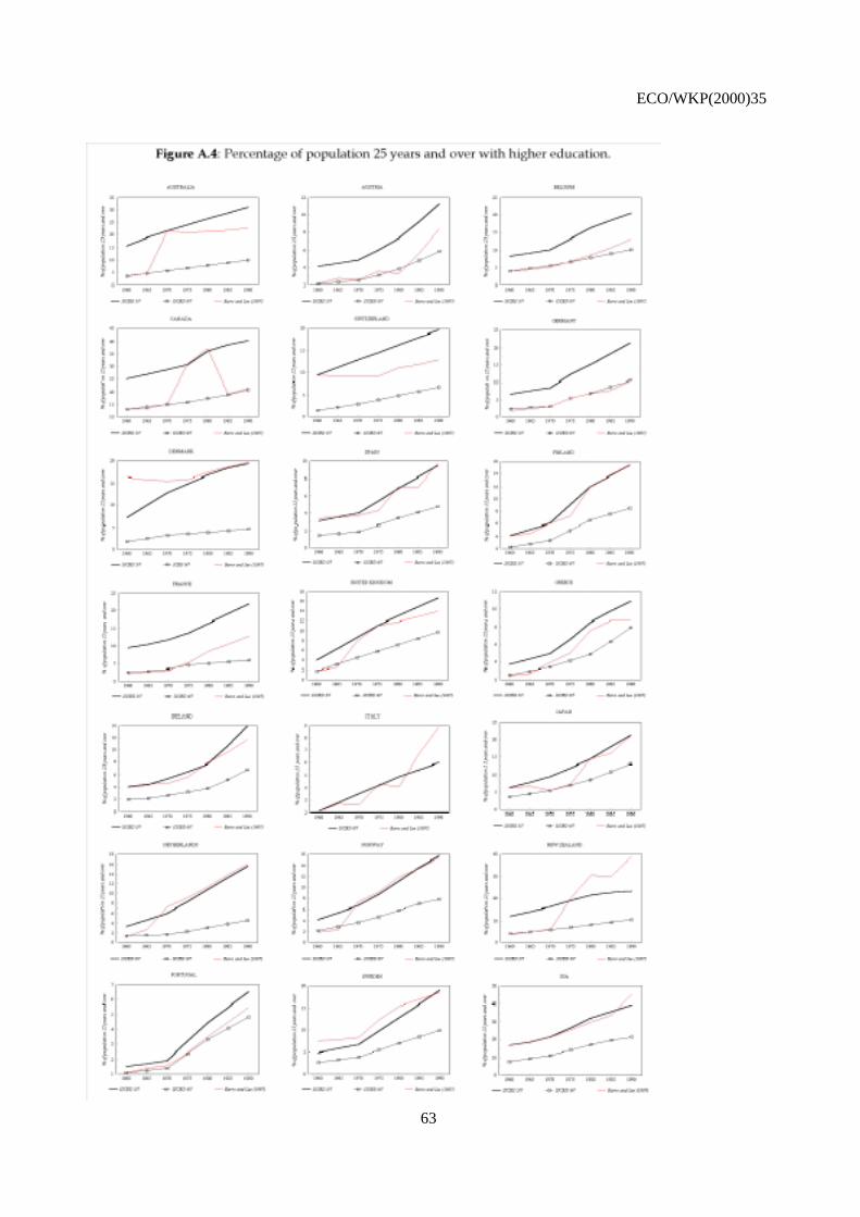
ECO/WKP(2000)35

63

ECO/WKP(2000)35

64

BIBLIOGRAPHY

BARRO, R. and J.W. LEE (1993), “International comparisons of educational attainment”, Journal ofMonetary Economics 32, pp. 363-94.

BARRO, R. and J.W. LEE (1994), “Sources of economic growth”, Carnegie-Rochester Conference Serieson Public Policy 40, pp. 1-46.

BARRO, R. and J.W. LEE (1996), “International measures of schooling years and schooling quality”,American Economic Review Papers and Proceedings 86(2), pp. 218-23.

BEHRMAN, J. and M. ROSENZWEIG (1994), “Caveat emptor: cross-country data on education and thelabor force”, Journal of Development Economics 44, pp. 147-71.

BENHABIB, J. and M. SPEIGEL (1994), “The role of human capital in economic development: evidencefrom aggregate cross-country data”, Journal of Monetary Economics 34, pp. 143-73.

CASELLI, F., G. ESQUIVEL and F. LEFORT (1996), “Reopening the convergence debate: a new look atcross-country growth empirics”, Journal of Economic Growth, pp. 363-89.

DE LA FUENTE, A. (1996), “On the sources of convergence: A close look at the Spanish regions”, CEPRDiscussion Paper No. 1543.

DE LA FUENTE, A. (2000), “Human capital and growth: a survey”, mimeo, Instituto de AnálisisEconómico, Barcelona.

DABÁN, T., R. DOMÉNECH and C. MOLINAS (1997), “International and intertemporal comparisons ofreal product in OECD countries: a growth sensitivity approach”, Review of Income andWealth 43(1), pp. 33-48.

GRILICHES, Z. (1980), “R&D and the productivity slowdown”, American Economic Review 70 (Papersand Proceedings), pp. 343-48.

GRILICHES, Z. and J. HAUSMAN (1986), “Errors in variables in panel data”, Journal ofEconometrics 31, pp. 93-118.

HAMILTON, J. and J. MONTEAGUDO (1998), “The augmented Solow model and the productivityslowdown”, Journal of Monetary Economics 42, pp. 495-509.

ISLAM, N. (1995), “Growth empirics: a panel data approach”, Quarterly Journal of Economics 110,pp. 1127-70.

JONES, Ch. (1997), “Convergence revisited”, Journal of Economic Growth 2, pp. 131-53.

ECO/WKP(2000)35

65

KANEKO, M. (1986), “The educational composition of the world’s population: a database”, WashingtonDC, the World Bank, Education and Training Department, Report No. EDT 29.

KLENOW, P. and A. RODRÍGUEZ-CLARE (1997), “The neo-classical revival in growth economics: hasit gone too far?” in B. Bernanke and J. Rotenberg, editors, Macroeconomics Annual 1997.Cambridge, MA. MIT Press, pp. 73-102.

KNIGHT, M., N. LOAYZA and D. VILLANUEVA (1993), “Testing the neo-classical theory of economicgrowth: A panel data approach”, IMF Staff Papers 40(3), pp. 512-41.

KYRIACOU, G. (1991), “Level and growth effects of human capital, A cross-country study of theconvergence hypothesis”, mimeo, NYU.

LAU, L., S. BHALLA and F. LOUAT (1991), “Human and physical capital stock in developing countries:construction of data and trends”, draft mimeo, World Development Report, World Bank.

LAU, L, D. JAMISON, and F. LOUAT (1991), “Education and productivity in developing countries: anaggregate production function approach”, report No. WPS 612, the World Bank.

MANKIW, G., D. ROMER and D. WEIL (1992), “A contribution to the empirics of economic growth”,Quarterly Journal of Economics, pp. 407-37.

NEHRU, V., E. SWANSON and A. DUBEY (1995), “A new database on human capital stocks indeveloping and industrial countries: sources, methodology and results”, Journal of DevelopmentEconomics, 46, pp. 379-401.

NORDIC STATISTICAL SECRETARIAT (1994), Educational Indicators in the Nordic Countries.

OECD (various years). Education at a Glance. Paris.

OECD (1974). Annuaire des Statistiques de l’Enseignement, Vol. I, Paris.

OECD (1970a). Statistics of the Occupational and Educational Structure of the Labour Force in53 Countries. Paris.

OECD (1970b). Development of Higher Education, 1950-67. Statistical Survey. Paris.

OECD (1990). L’Enseignement dans les Pays de l’OCDE, 1987-88. Recueil d’informations statistiques.Paris.

OECD (1995). OECD Education Statistics 1985-92. Paris.

PRESCOTT, E. (1998), “Needed: A theory of total factor productivity”, International EconomicReview 39(3), pp. 525-51.

PRITCHETT, L. (1995), “Where has all the education gone?”, mimeo, World Bank.

PSACHAROPOULOS, G. and A. ARRIAGADA (1986), “The educational composition of the labourforce: an international comparison”, International Labour Review 125(5), Sept.-Oct., pp. 561-74.

STEEDMAN, H. (1996), “Measuring the quality of educational outputs: a note”, Centre for EconomicPerformance, Discussion Paper No. 302, LSE.

ECO/WKP(2000)35

66

TEMPLE, J. (1998), “Robustness tests of the augmented Solow model”, Journal of AppliedEconometrics 13, pp. 361-75.

UNESCO (1993). Statistics of Educational Attainment and Illiteracy, 1970-80. Division of Statistics onEducation. UNESCO, Paris.

UNESCO (various years). Statistical Yearbook, Paris.

UNITED NATIONS (various years). Demographic Yearbook, New York.

ECO/WKP(2000)35

67

ECONOMICS DEPARTMENT

WORKING PAPERS

261. Raising the Speed Limit: US Economic Growth in the Information Age(October 2000) Dale W. Jorgenson and Kevin J. Stiroh

260. Summary of an Informal Workshop on the Causes of Economic Growth(October 2000) Jonathan Temple

259. Knowledge, Technology and Economic Growth: Recent Evidence from OECD Countries(October 2000) Andrea Bassanini, Stefano Scarpetta and Ignazio Visco

258. Average Effective Tax Rates on Capital, Labour and Consumption(October 2000) David Carey and Harry Tchilinguirian

257. The Health Care System in Poland(September 2000) Nathalie Girouard and Yutaka Imai

256. Public Expenditure Reform: The Health Care Sector in the United Kingdom(August 2000) Vincent Koen

255. Regulatory Reform in Road Freight and Retail Distribution(August 2000) Olivier Boylaud

254. Regulation, Market Structure and Performance in Air Passenger Transportation(August 2000) Rauf Gonenc and Giuseppe Nicoletti

253. Policy Interdependence during Economic Transition: the Case of Slovakia 1999-2000(June 2000) Joaquim Oliveira Martins and Tristan Price

252. E-Commerce: Impacts and Policy Challenges(June 2000) Jonathan Coppel

251. The Implementation and the Effects of Regulatory Reform: Past Experience and Current Issues(June 2000) Rauf Gonenc, Maria Maher and Giuseppe Nicoletti

250. The Concept, Policy Use and Measurement of Structural Unemployment: Estimating a Time Varying NAIRUacross 21 OECD Countries(June 2000) Pete Richardson, Laurence Boone, Claude Giorno, Mara Meacci, David Rae and David Turner

249. Options for Reforming the Spanish Tax System(June 2000) Isabelle Joumard and Aristomène Varoudakis

248. Economic Growth in the OECD Area: Recent Trends at the Aggregate and Sectoral Level(June 2000) Stefano Scarpetta, Andrea Bassanini, Dirk Pilat and Paul Schreyer

247. Economic Effects on the 1999 Turkish Earthquakes: an Interim Report(June 2000) Alexandra Bibbee, Rauf Gonenc, Scott Jacobs, Josef Konvitz and Robert Price

246. Policy Influences on Economic Growth in OECD Countries: an Evaluation of the Evidence(June 2000) Sanghoon Ahn and Philip Hemmings

ECO/WKP(2000)35

68

245. The Tax System in the Czech Republic(May 2000) Chiara Bronchi and Andrew Burns

244. The Tax System in Norway: Past Reforms and Future Challenges(May 2000) Paul van den Noord

243. A Changing Financial Environment and the Implications for Monetary Policy(May 2000) Paul Mylonas, Sebastian Schich, Gert Wehinger

242. Carbon Emission Leakages: a General Equilibrium View(May 2000) Jean-Marc Burniaux and Joaquim Oliveira Martins

241. The Healthcare System in Hungary(April 2000) Eva Orosz and Andrew Burns

240. Comparing Semi-Structural Methods to Estimate Unobserved Variables: the HPMV and Kalman FiltersApproaches(April 2000) Laurence Boone

239. New Issues in Public Debt Management: Government Surpluses in Several OECD Countries, the CommonCurrency in Europe and Rapidly Rising Debt in Japan(April 2000) Paul Mylonas, Sebastian Schich, Thorsteinn Thorgeirsson and Gert Wehinger

238. Regulation, Industry Structure and Performance in the Electricity Supply Industry(April 2000) Faye Steiner

237. Regulation, Market Structure and Performance in Telecommunications(April 2000) Olivier Boylaud and Giuseppe Nicoletti

236. Predicting the Evolution and Effects of the Asia Crisis from the OECD Perspective(April 2000) Pete Richardson, Ignazio Visco and Claude Giorno

235. Modelling Manufacturing Export Volumes EquationsA System Estimation Approach(April 2000) Keiko Murata, David Turner, David Rae and Laurence Le Fouler

234. The Polish Tax Reform(March 2000) Patrick Lenain and Leszek Bartoszuk

233. The Tax System in Mexico: a Need for Strengthening the Revenue Raising Capacity(March 2000) Thomas Dalsgaard

232. EMU, the Euro and the European Policy Mix(February 2000) Jonathan Coppel, Martine Durand and Ignazio Visco

231. The Tax System in Japan: a Need for Comprehensive Reform(February 2000) Thomas Dalsgaard and Masaaki Kawagoe

230. The Size and Role of Automatic Fiscal Stabilisers in the 1990s and Beyond(January 2000) Paul van den Noord

229. Enhancing Environmentally Sustainable Growth in Finland(January 2000) Ann Vourc’h and Miguel Jimenez

human capital in growth regressions: how much …search.oecd.org/economy/outlook/1885692.pdf ·...

Documents