hunting the potassium geoneutrinos with liquid
TRANSCRIPT

Hunting the Potassium Geoneutrinos with Liquid Scintillator CherenkovNeutrino Detectors
Zhe Wanga,b,∗, Shaomin Chena,b
aDepartment of Engineering Physics, Tsinghua University, Beijing 100084, ChinabCenter for High Energy Physics, Tsinghua University, Beijing 100084, China
Abstract
The research of geoneutrino is a new interdisciplinary subject of particle experiments and geo-science. Potassium-40(40K) decays contribute roughly 1/3 of the radiogenic heat of the Earth, but it is still missing from the experimentalobservation. Solar neutrino experiments with liquid scintillators have observed uranium and thorium geoneutrinos andare the most promising in the low-background neutrino detection. In this article, we present the new concept of usingliquid-scintillator Cherenkov detectors to detect the neutrino-electron elastic scattering process of 40K geoneutrinos.Liquid-scintillator Cherenkov detectors using a slow liquid scintillator can achieve this goal with both energy anddirection measurements for charged particles. Given the directionality, we can significantly suppress the dominantintrinsic background originating from solar neutrinos in conventional liquid-scintillator detectors. We simulated thesolar- and geo-neutrino scatterings in the slow liquid scintillator detector, and implemented energy and directionalreconstructions for the recoiling electrons. We found that 40K geoneutrinos can be detected with three standarddeviation accuracy in a kiloton-scale detector.
Keywords: Liquid-scintillator Cherenkov detector, Slow liquid scintillator, Geoneutrino, 40K neutrino
The interaction of neutrinos with matter is extremelyweak, so they easily penetrate celestial bodies.Determining the neutrino spectrum and flavor can shedlight on the production reaction and environment. Theyare thus ideal probes of the Earth and Sun. Geoneutrinosare primarily generated by three types of long-livedradioactive isotopes, potassium-40 (40K), uranium-238(238U), and thorium-232 (232Th). Their origins,compositions, and distributions are very interestingquestions in geoscience. They can help to discover thephysical and chemical structure of the Earth and even toreveal its evolution.
The KamLAND [1–4] and Borexino [5–7]experiments have made pioneering contributions togeoneutrino discovery. The detection is achievedby finding inverse-beta-decay, IBD, signals inliquid-scintillator detectors. An IBD signal consists ofa prompt positron signal and a delayed neutron-capturesignal, and the prompt-delay-coincidence provides aclear signature of the interaction. The IBD cross-sectionis relatively high. The energy threshold for the reaction
∗Email: [email protected]
is 1.8 MeV, and only 232Th and 238U geoneutrinos areaccessible. Almost no directional information can beextracted for the initial neutrinos [8].
Neutrinos originating in the mantle have a directconnection with the power that drives the platetectonics and mantle convection [9, 10]. However, themeasurements of mantle geoneutrinos rely heavily onthe crust geoneutrino predictions. Consequently, themantle component still has considerable uncertainty.In [11], Tanaka and Watanabe proposed to usea 6Li-load liquid scintillator to extract directionalinformation about U and Th neutrinos using the IBDprocess, and even to image the Earth’s interior.
The K element is more mysterious than U and Th.Potassium-40 (40K) decays contribute roughly 1/3 of theradiogenic heat of the Earth, but no experimental 40Kneutrino result has been reported. And because K isa volatile element, precipitating it into typical mineralphases is more difficult than for U or Th. Measuring theflux of 40K neutrinos versus 238U and 232Th neutrinoscan offer input to understanding the formation processof the Earth [12]. The model of 40K and 40Ar in the airand the Earth also indicates the enriched and depleted
Preprint submitted to CPC April 9, 2020
arX
iv:1
709.
0374
3v4
[he
p-ex
] 8
Apr
202
0

mantle structure [13]. In [14], Leyton, Dye, and Monroeproposed to use directional neutrino detectors, likenoble-gas time-projection chambers to explore variousgeoneutrino components.
Note that, so far, the liquid scintillator detector ofBorexino is the only one achieving sub-MeV neutrinospectroscopy, where both large target mass and lowbackground are realized. Solar neutrinos are detectedthrough neutrino-electron scattering,
ν + e− → ν + e−, (1)
which has no theoretical threshold. There is astrong correlation between the initial neutrino andscattered electron direction, especially after imposinga requirement on the kinetic energy of the recoilingelectron. In this paper, we consider introducingdirectionality to the conventional liquid scintillatordetector to suppress the intrinsic solar neutrinobackground and to detect the 40K geoneutrinos.
Because of the long emission time constant ofscintillation radiation, the new type of liquid-scintillatorCherenkov neutrino detectors [15–17] can identify thesmall prompt Cherenkov radiation from huge slowscintillation light. This unique feature can providenot only the reconstruction of both direction andenergy which has never been achieved in conventionalliquid scintillation neutrino detectors but also particleidentification [18]. We consider two schemes for theliquid-scintillator Cherenkov neutrino detector. Thefirst approach is to use a fast, high light-yield liquidscintillator and fast photon detectors. In this case,the light yield can reach 10,000 photons per MeVwith an emission time constant of a few nanoseconds,which is much longer than several picoseconds oftiming precision of the photon detectors. The recentexperimental development for this approach can befound in references [19–21]. The second approach is touse a slow liquid scintillator and photomultiplier tubes(PMTs). The PMTs usually have a timing precision ofabout one nanosecond, while the emission time constantfor the slow liquid scintillator is much longer, forexample, 20 nanoseconds [22–24].
In this article, we focus on the latter scheme. Weadopted the parameter set for pure linear alkylbenzene(LAB) [22] as a slow liquid-scintillator candidate,which is most favorable for Cherenkov separation. Thelight yield is 2530 photons/MeV, and the emission riseand decay time constants are 12.2 ns and 35.4 ns,respectively. The time profile is shown in Figure 1.The Cherenkov threshold is 0.178 MeV, assuming therefractive index of the liquid to be 1.49 [25].
0 10 20 30 40 50 60 70 80 90 100
Time [ns]
0
0.0005
0.001
0.0015
0.002
0.0025
0.003
0.0035
0.004
Ligh
t yie
ld
Figure 1: The normalized time profile of scintillation light emitted bythe slow liquid scintillator, LAB [22].
1. Analysis and Result
1.1. Ideal Expectation with a Terrestrial DetectorWe consider an ideal terrestrial detector, located on
the Earth’s equator, rotates along with the Earth. Wedefine solar z-axis, z�, from the Sun to the Earth,and an Earth z-axis, z⊕, from the center of the Earthto the detector (see Figure 2). Correspondingly, wedefine the angle between the recoiling electron and z�as θ� and the angle with z⊕ as θ⊕. Geoneutrinos andsolar neutrinos are generated and the kinetic energiesof the recoiling electrons are recorded. With a cuton the recoiling electron kinetic energy at 0.7 MeV,the distributions of cos θ� and cos θ⊕ for the remainingneutrinos are shown in Figure 3. The geoneutrinos(crust and mantle) are clearly separated from thesolar-neutrino background. Since the energy range ofthe 40K neutrinos is distinguishable from those of the232Th and 238U neutrinos, there is a chance to detect the40K component. Next, we will consider a real detector.
Figure 2: Definitions of z�, z⊕, θ�, and θ⊕. The yellow cube representsthe neutrino detector.
2

1− 0.8− 0.6− 0.4− 0.2− 0 0.2 0.4 0.6 0.8 1
⊕θcos
1−
0.8−
0.6−
0.4−0.2−
0
0.2
0.4
0.6
0.8
1θco
s
Solar
Crust
Mantle
Figure 3: Theoretical distributions of cos θ� and cos θ⊕ for solar,crust and mantle neutrinos when the kinetic energies of the recoilingelectrons are required to exceed 0.7 MeV.
1.2. Liquid-Scintillator Cherenkov Detector Simulation
Figure 4: Detector concept. From inside to outside are the slow liquidscintillator (yellow), water (blue), PMT, and water again.
We adopted the detector scheme [26] shown inFigure 4. In the center is the slow liquid scintillator,which is contained in a transparent container, and itis surrounded by a non-scintillating material, such aswater or mineral oil. The PMTs are installed withall photocathodes facing inward and forming a largespherical array. The PMTs are all immersed in the wateror oil. The water behind the PMTs also serves as a vetolayer, shielding the detector from radioactivities likebetas, gammas, neutrons, and cosmic-ray muons. Thenumber of signals is directly proportional to the targetmass, and due to the required low-background rate, onlythe central region of the liquid scintillator known as thefiducial volume is accepted for signal detection.
The simulation of solar-neutrino generation,geo-neutrino generation, and neutrino-electron
scattering are described in Appendix A, Appendix B,and Appendix C, respectively. The recoil electronsare simulated using Geant4 [27–29] including allpossible electromagnetic processes. Because ofmultiple scattering, the initial direction of the electronis smeared out. Some electrons eventually turn back,when they are close to stopping.
Both Cherenkov and scintillation light emissionsare handled by Geant4; however, the production ofscintillation light is customized according to LABmeasurement [22].
All the optical photons are recorded and gonethrough empirical simulations [26, 30], because theattenuation length of optical photons still needs moreexperimental research [22], and the target mass orvolume is a parameter we want to test. The limitedPMT photocathode coverage and photon attenuationand scattering will cause efficiency loss, so we assumepractically only 66.7% (2/3) of the photons can reachthe PMTs. The quantum efficiency of a PMT is assumedto be 30% for all photons within the range [300, 550]nm and to be zero for the rest, which is motivatedby the high quantum efficiency of PMTs, accordingto [31]. In summary, the total efficiency for generatingphotoelectron, PE, is 20% for photons within the range[300, 550] nm and is zero outside of this wavelengthrange.
1.3. Energy and Direction Reconstruction
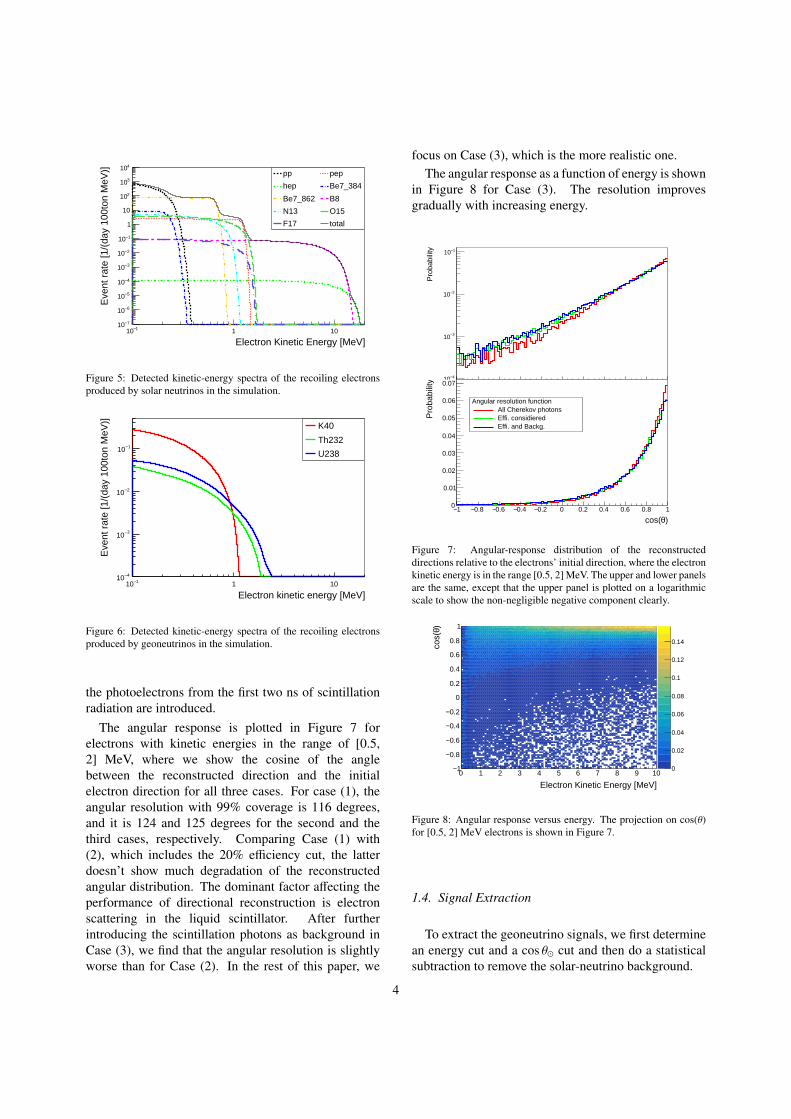
From the simulation, we can determine the averageenergy scale, i.e., the number of PE per MeV, and withthat, the total number of detected PEs for each eventis scaled to the detected energy. The detected-energyspectra of solar- and geo-neutrinos are shown inFigure 5 and Figure 6, respectively.
We use a weighted-center method to reconstruct thedirection of the recoiling electrons, ~R. The formula is
~R =1
NPE
NPE∑i=1
~ri, (2)
where ~ri is the direction of each photoelectron and NPEis the number of photoelectrons.
We tried three groups of photons. In Case (1)we use all Cherenkov photons to study the best caseand to understand the scattering of electrons in theliquid scintillator. In Case (2) we apply the 20%efficiency cut as described in Section 1.2. We usethis study to understand the results with Cherenkovphotons only. In Case (3), we tested a more realisticcase, where the detection efficiency is considered, and
3
1−10 1 10
Electron Kinetic Energy [MeV]
7−10
6−10
5−10
4−10
3−10
2−10
1−10
1
10
210
310
410
Eve
nt r
ate
[1/(
day
100t
on M
eV)] pp pep
hep Be7_384
Be7_862 B8
N13 O15
F17 total
Figure 5: Detected kinetic-energy spectra of the recoiling electronsproduced by solar neutrinos in the simulation.
1−10 1 10
Electron kinetic energy [MeV]
4−10
3−10
2−10
1−10
Eve
nt r
ate
[1/(
day
100t
on M
eV)] K40
Th232
U238
Figure 6: Detected kinetic-energy spectra of the recoiling electronsproduced by geoneutrinos in the simulation.
the photoelectrons from the first two ns of scintillationradiation are introduced.
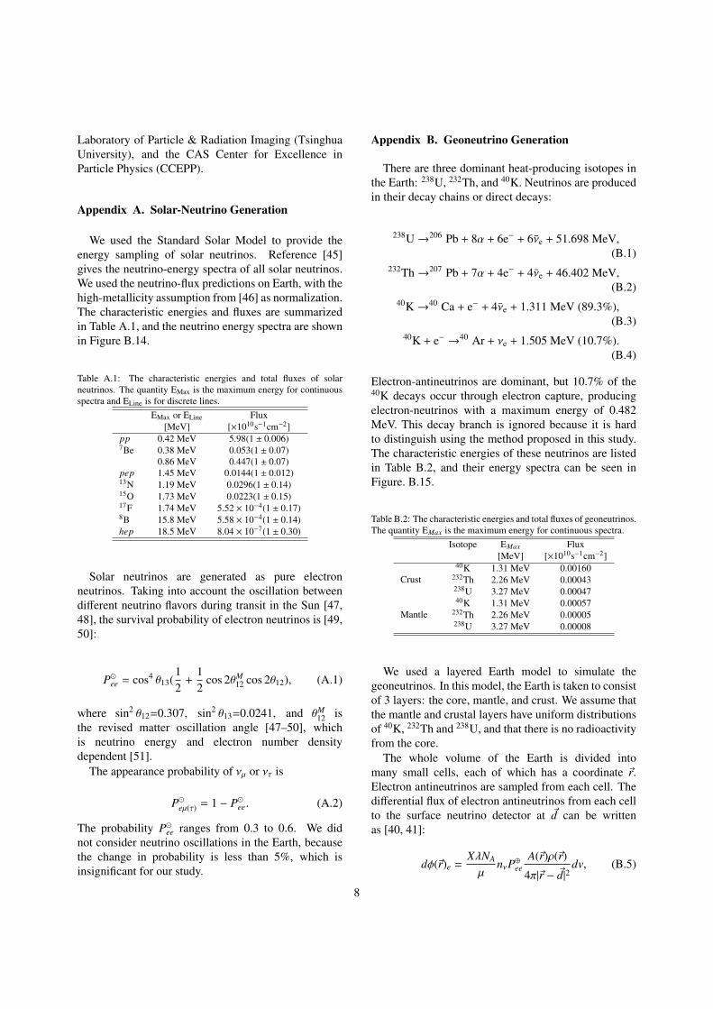
The angular response is plotted in Figure 7 forelectrons with kinetic energies in the range of [0.5,2] MeV, where we show the cosine of the anglebetween the reconstructed direction and the initialelectron direction for all three cases. For case (1), theangular resolution with 99% coverage is 116 degrees,and it is 124 and 125 degrees for the second and thethird cases, respectively. Comparing Case (1) with(2), which includes the 20% efficiency cut, the latterdoesn’t show much degradation of the reconstructedangular distribution. The dominant factor affecting theperformance of directional reconstruction is electronscattering in the liquid scintillator. After furtherintroducing the scintillation photons as background inCase (3), we find that the angular resolution is slightlyworse than for Case (2). In the rest of this paper, we
focus on Case (3), which is the more realistic one.The angular response as a function of energy is shown
in Figure 8 for Case (3). The resolution improvesgradually with increasing energy.
1− 0.8− 0.6− 0.4− 0.2− 0 0.2 0.4 0.6 0.8 1
)θcos(
4−10
3−10
2−10
1−10
Pro
babi
lity
1− 0.8− 0.6− 0.4− 0.2− 0 0.2 0.4 0.6 0.8 1
)θcos(
0
0.01
0.02
0.03
0.04
0.05
0.06
0.07
Pro
babi
lity
Angular resolution functionAll Cherekov photonsEffi. considieredEffi. and Backg.
Figure 7: Angular-response distribution of the reconstructeddirections relative to the electrons’ initial direction, where the electronkinetic energy is in the range [0.5, 2] MeV. The upper and lower panelsare the same, except that the upper panel is plotted on a logarithmicscale to show the non-negligible negative component clearly.
0
0.02
0.04
0.06
0.08
0.1
0.12
0.14
0 1 2 3 4 5 6 7 8 9 10
Electron Kinetic Energy [MeV]
1−
0.8−
0.6−
0.4−
0.2−
0
0.2
0.4
0.6
0.8
1)θco
s(
Figure 8: Angular response versus energy. The projection on cos(θ)for [0.5, 2] MeV electrons is shown in Figure 7.
1.4. Signal Extraction
To extract the geoneutrino signals, we first determinean energy cut and a cos θ� cut and then do a statisticalsubtraction to remove the solar-neutrino background.
4

1.4.1. Determination of the Signal RegionThe event rate ratio of geo to solar neutrinos as a
function of energy is shown in Figure 9, according towhich we define three observation windows. One is theenergy range [0.7, 2.3] MeV, where all 40K, 232Th, and238U geoneutrinos provide contributions. The second isthe range [0.7, 1.1] MeV, which is dominated by 40Kneutrinos, and the third is the range [1.1, 2.3] MeV,which is populated by 232Th and 238U neutrinos. For theevents below 0.7 MeV, like the νe component from 40Kdecay, the directional reconstruction is rather poor, andthese events are not usable. For all the three observationwindows, the solar-neutrino background needs to besuppressed by a factor of 100-200 in order to enable usto extract the geoneutrino signals. In the [0.7, 1.1] MeVwindow, the dominant solar-neutrino backgrounds arethe pep, 13N, and 15O neutrinos, while the 15O and 8Bneutrinos are in the [1.1, 2.3] MeV window.
0.5 1 1.5 2 2.5 3 3.5 4
Electron kinetic energy [MeV]
0
0.005
0.01
0.015
0.02
0.025
Eve
nt r
ate
ratio Geo to solar event rate ratio
With true recoil energy
With smeared recoil energy
Figure 9: Signal-to-background ratio (geo-to-solar-neutrino ratio) asa function of the kinetic energy of the electron.
We next determine the cos θ� cut. After applying thedetected-energy cut of [0.7, 2.3] MeV, the cos θ� of theremaining solar- and geo- neutrinos are both plotted inFigure 10. With a cut at cos θ� < −0.75, the solarneutrinos are suppressed by a factor of 150, and thesignal (geo) to background (solar) ratio is about 0.1,closer to unity than the other region.
1.4.2. Signal MeasurementUsing the data sample from our imagined
experiment, the number of geoneutrino signals,Ngeo, can be calculated by subtracting the solar-neutrinobackground:
Ngeo = Ncan − Nbkg × ε, (3)
where Ncan is the number of all candidates, Nbkg is thebackground flux, e.g., the solar neutrinos, and ε is the
1− 0.8− 0.6− 0.4− 0.2− 0 0.2 0.4 0.6 0.8 1θcos
1
10
210
310
410
Ent
ries/
0.00
5
Solar neutrinos
Geo neutrinos
Figure 10: The cos θ� distributions of the simulated solar and geoneutrinos, where the total statistics are for a 3 kt detector and a 20-yearobservation period, and a detected energy cut at [0.7, 2.3] MeV isapplied.
detection efficiency, including the energy-window cutand the cos θ� cut.
The uncertainty σgeo in the geoneutrino counts is
σgeo =
√σ2
candidate + N2solarσ
2ε + ε2σ2
solar, (4)
where, σcandidate is the statistical uncertainty of the datasample, σsolar is the solar-neutrino-flux uncertainty, andσε is the uncertainty in the efficiency.
For the solar-neutrino background, the pep and B8neutrinos are dominant. We expect several proposedexperimental approaches, like Jinping [32], LENA [33],THEIA [17], and [34], will improve their uncertainty toa 1% precision. Calibration sources can be deployed tomultiple locations of the detector [35]. The calibrationsource can be a beta source enclosed in a small metalbox with a small pinhole as a collimator. With enoughstatistics, a 1% precision is expected.
From our experience, we assume that thedetection-efficiency uncertainty, including the energyand the cos θ� cuts, can also reach 1%.
For the 40K energy window, we need in addition tosubtract the 238U and 232Th geoneutrino componentsas backgrounds. With the advantage of lowreactor-neutrino background, the Jinping NeutrinoExperiment can measure the total flux of these neutrinosto better than 5%.
1.5. Sensitivity Curve
From the discussion above and the results for angularresolution and expected systematic uncertainties, wecan now estimate the precision of the geoneutrino-flux
5

measurement as a function of exposure. We express thesensitivity as
sensitivity = Ngeo/σgeo, (5)
which gives the relative precision, or the deviation fromthe null assumption. The study is performed for eachof the three energy windows defined in Section 1.4.1above: one for all geoneutrinos, [0.7, 2.3] MeV, anotherfor the 40K geoneutrinos, [0.7, 1.1] MeV, and the thirdfor the 238U and 232Th components, [1.1, 2.3] MeV, Theresults are shown in Figure 11, Figure 12, and Figure 13,respectively.
Among these results, the most attractive is for the40K geoneutrinos, Figure 12. With a three-kiloton targetmass and 20-year data-taking time, a 3-σ observation ispossible. With a 20-kiloton detector, a 5-σ observationis expected.
For the 232Th and 238U region, even with the bettersignal-to-background ratio shown in Figure 9, the resultis still limited by low statistics. So the expectation isworse than for the 40K geoneutrinos.
2. Discussion
The key aspects of this study are highlighted below,and the important properties of them will be discussed.We generated the solar and geoneutrinos according tomodels, and propagated the neutrinos to a detectoron the Earth’s equator, taking into account neutrinooscillations. Neutrino-electron elastic scattering issimulated using standard theoretical formulas. Thetransport of the recoil electrons and the production ofCherenkov and scintillation photons are all handled byGeant4, using the customized light yield and rise anddecay time constants of LAB. Photoelectron detectionis sampled according to a 20% detection efficiencyfor a certain wavelength range. The number ofphotoelectrons in each event is scaled to reconstruct therecoiling electron’s kinetic energy. A weighted-centermethod is applied to reconstruct the directions of theelectrons. With the reconstructed energy and directionaldistributions, we then determined the cuts required toextract geoneutrinos and to remove most of the solarneutrino background. The remaining solar-neutrinobackground is subtracted statistically from the finalsample. We then scanned the exposure to see whether itis possible to discover geoneutrinos with this technique.We elaborate on some features of this study below.
2.1. Neutrino-Electron ScatteringFor this detection scheme, the directional
reconstruction of the recoil electrons is crucial for
0 200 400 600 800 1000
Exposure [kt.year]
2
2.5
3
3.5
4
4.5
5
5.5
6
Sen
sitiv
ity [s
igm
a]
Figure 11: Discovery sensitivity for all geoneutrinos as a function ofexposure.
0 200 400 600 800 1000
Exposure [kt.year]
2
2.5
3
3.5
4
4.5
5
5.5
Sen
sitiv
ity [s
igm
a]
Figure 12: Discovery sensitivity for 40K geoneutrinos as a function ofexposure.
0 200 400 600 800 1000
Exposure [kt.year]
1
2
3
4
5
6
7
Sen
sitiv
ity [s
igm
a]
Figure 13: Discovery sensitivity for 238U and 232Th genoneutrinos asa function of exposure.
the overall performance. The angular resolutiongoverns the final signal-to-background ratio. We findthat the scattering of the electrons in the LAB has theprimary effect on the resolution. Reconstruction witha limited number of Cherenkov photoelectrons is onlythe secondary factor, as presented. The density of the
6

LAB is 0.87 × 10³ kg/m3. A further simulation studyshows that the angular resolution exhibits no significantimprovement unless the density is close to the gaseousstate.
2.2. Slow Liquid Scintillator
In this study, we assumed a 66.7% detectionefficiency, considering the PMT photocathode coverage,photon attenuation in the detector, and a 30% quantumefficiency for photons in the range [300, 550] nm. Thedetection efficiency is the most optimistic assumptionin this entire study. The scintillation emission spectrumof the pure LAB peaks at 340 nm [22], which is closeto the UV side and may suffer more absorption thanwe expected. The absorption is caused by the intrinsicabsorption band of LAB and it cannot be resolved bypurification. With the addition of wavelength-shiftingmaterials, the peak can be shifted into the visiblerange. The absorption could be severer and somepart of the Cherenkov light can be lost. We hopethat this investigation will stimulate further relevantslow-liquid-scintillator research, for example, to searcha new solvent and a new wavelength shifter.
2.3. Other Background
In this study, we included the critical solar-neutrinobackground, but other intrinsic or environmentalradiative backgrounds should be considered too. Wetake the situation of solar neutrino study at the Borexinoexperiment as an example [36, 37] to explain ourexpectations. The radioactive 10C and 11C backgroundare induced by cosmic-ray muons. At a deeper site,like the Jinping underground laboratory [32], thesebackgrounds will be suppressed by a factor of 100 ormore and become negligible. External photons affectthe signal extraction, for example from 208Tl, and thiscan be avoided by a tighter fiducial volume cut. For theinternal background, the decay products of the U andTh with secular equilibrium are not significant. Onething worth special attention is the 210Bi background.After a few rounds of liquid scintillator purificationwith distillation, gas and water stripping and longterm monitoring, the remaining 210Bi seems originallyfrom radon gas absorption on detector inner surfaceand is leaching out by radon’s daughter nuclei 210Pb.Good progress has been made by suppressing thethermal convection of the liquid scintillator [38, 39].Surface cleaning was also mentioned to suppress theinitial radon contamination. These effects shouldbe considered later in developing a more realisticexperimental design.
Reactor-neutrino backgrounds can be avoidedby selecting an experimental site far away fromcommercial reactors, like the Jinping undergroundlaboratory [32, 40, 41]. Reactor-neutrino fluxes also canbe well constrained to be better than 6% [35, 42–44].The reactor-neutrino background can also be measuredin-situ, so this is not a critical issue.
2.4. Mantle Neutrinos
Knowledge of mantle neutrinos also is necessary.However, it is only about 30% of the total geoneutrinoflux if the detector is placed on a continental site, whilethe rest originates from the crust. Given the currentsensitivity in measuring the total flux and the currentangular resolution, we did not pursue this issue further.
3. Conclusion
K element is volatile and its concentration in theEarth is not in balance with the refractory U andTh elements. A measurement of the K element inthe Earth is of interest to understand the chemicalevolution of the Earth. The detection of 40K neutrinosmay lead to new knowledge of the Earth. Previouslyonly U and Th geoneutrinos can be detected with theinverse beta process with a 1.8 MeV threshold. 40Kgeoneutrinos are hard to discover for its low energy andhigh solar neutrino background. In this work, we foundthat liquid scintillator Cherenkov neutrino detectorscan be used to detect the 40K geoneutrinos. Liquidscintillator Cherenkov detectors feature both energyand direction measurements for charged particles.With the elastic scattering process of neutrinos withelectrons, 40K geoneutrinos can be detected without anyintrinsic physical threshold. With the directionality,the dominant intrinsic background originated from solarneutrinos in common liquid scintillator detectors canbe suppressed. With the studies of MeV electrons ofGeant4 simulation, quantum and detection efficiency,and Cherenkov direction reconstruction, it is found thatwe can detect 40K energy geoneutrinos with 3 standarddeviations with a kilo-ton scale detector. In this study,the setting of parameters is on the optimistic side, but wefound that this technology is worth further development.
4. Acknowledgement
This work is supported in part by the National NaturalScience Foundation of China (Nos. 11620101004,11235006, 11475093), the Ministry of Science andTechnology of China (no. 2018YFA0404102), the Key
7
Laboratory of Particle & Radiation Imaging (TsinghuaUniversity), and the CAS Center for Excellence inParticle Physics (CCEPP).
Appendix A. Solar-Neutrino Generation
We used the Standard Solar Model to provide theenergy sampling of solar neutrinos. Reference [45]gives the neutrino-energy spectra of all solar neutrinos.We used the neutrino-flux predictions on Earth, with thehigh-metallicity assumption from [46] as normalization.The characteristic energies and fluxes are summarizedin Table A.1, and the neutrino energy spectra are shownin Figure B.14.
Table A.1: The characteristic energies and total fluxes of solarneutrinos. The quantity EMax is the maximum energy for continuousspectra and ELine is for discrete lines.
EMax or ELine Flux[MeV] [×1010s−1cm−2]
pp 0.42 MeV 5.98(1 ± 0.006)7Be 0.38 MeV 0.053(1 ± 0.07)
0.86 MeV 0.447(1 ± 0.07)pep 1.45 MeV 0.0144(1 ± 0.012)13N 1.19 MeV 0.0296(1 ± 0.14)15O 1.73 MeV 0.0223(1 ± 0.15)17F 1.74 MeV 5.52 × 10⁻⁴(1 ± 0.17)8B 15.8 MeV 5.58 × 10⁻⁴(1 ± 0.14)hep 18.5 MeV 8.04 × 10⁻⁷(1 ± 0.30)
Solar neutrinos are generated as pure electronneutrinos. Taking into account the oscillation betweendifferent neutrino flavors during transit in the Sun [47,48], the survival probability of electron neutrinos is [49,50]:
P�ee = cos4 θ13(12
+12
cos 2θM12 cos 2θ12), (A.1)
where sin2 θ12=0.307, sin2 θ13=0.0241, and θM12 is
the revised matter oscillation angle [47–50], whichis neutrino energy and electron number densitydependent [51].
The appearance probability of νµ or ντ is
P�eµ(τ) = 1 − P�ee. (A.2)
The probability P�ee ranges from 0.3 to 0.6. We didnot consider neutrino oscillations in the Earth, becausethe change in probability is less than 5%, which isinsignificant for our study.
Appendix B. Geoneutrino Generation
There are three dominant heat-producing isotopes inthe Earth: 238U, 232Th, and 40K. Neutrinos are producedin their decay chains or direct decays:
238U→206 Pb + 8α + 6e− + 6νe + 51.698 MeV,(B.1)
232Th→207 Pb + 7α + 4e− + 4νe + 46.402 MeV,(B.2)
40K→40 Ca + e− + 4νe + 1.311 MeV (89.3%),(B.3)
40K + e− →40 Ar + νe + 1.505 MeV (10.7%).(B.4)
Electron-antineutrinos are dominant, but 10.7% of the40K decays occur through electron capture, producingelectron-neutrinos with a maximum energy of 0.482MeV. This decay branch is ignored because it is hardto distinguish using the method proposed in this study.The characteristic energies of these neutrinos are listedin Table B.2, and their energy spectra can be seen inFigure. B.15.
Table B.2: The characteristic energies and total fluxes of geoneutrinos.The quantity EMax is the maximum energy for continuous spectra.
Isotope EMax Flux[MeV] [×1010s−1cm−2]
Crust
40K 1.31 MeV 0.00160232Th 2.26 MeV 0.00043238U 3.27 MeV 0.00047
Mantle
40K 1.31 MeV 0.00057232Th 2.26 MeV 0.00005238U 3.27 MeV 0.00008
We used a layered Earth model to simulate thegeoneutrinos. In this model, the Earth is taken to consistof 3 layers: the core, mantle, and crust. We assume thatthe mantle and crustal layers have uniform distributionsof 40K, 232Th and 238U, and that there is no radioactivityfrom the core.
The whole volume of the Earth is divided intomany small cells, each of which has a coordinate ~r.Electron antineutrinos are sampled from each cell. Thedifferential flux of electron antineutrinos from each cellto the surface neutrino detector at ~d can be writtenas [40, 41]:
dφ(~r)e =XλNA
µnνP⊕ee
A(~r)ρ(~r)
4π|~r − ~d|2dv, (B.5)
8

Table B.3: Element abundance of K, Th and U in the mantle and crustused for this study.
K [kg/kg] Th [kg/kg] U [kg/kg]Crust 1.16 × 10⁻² 5.25 × 10⁻⁶ 1.35 × 10⁻⁶
Mantle 152 × 10−6 21.9 × 10⁻⁹ 8.0 × 10⁻⁹
where X is the natural isotopic mole fraction of eachisotope, λ is the corresponding decay constant, NA isthe Avogadro’s number, µ is the atomic mole mass,nν is the number of neutrinos per decay, P⊕ee is theaverage survival probability, A(~r) is the abundance ofeach element in kg/kg, ρ(~r) is the local density at eachlocation, and |~r − ~d| gives the distance from each cell ~rto our detector at ~d.
We take the outer radii of the core, mantle and crustto be 3480, 6321, and 6371 km [52], respectively, withthe corresponding densities to be 11.3, 5.0, and 3.0g/cm3. The element abundance values of K, Th andU are set to match the integrated flux predictions, asin [40, 41], and the values are given in Table B.3.This simplified layered model is not as sophisticatedas that in reference [53], but it is sufficient for ourdemonstration purposes. The rest of the parametersare taken from reference [41]. The total fluxes of thepredicted geoneutrinos are summarized in Table B.2.The non-oscillating neutrino spectra of 40K, 232Th and238U at the detection site are shown in Figure. B.15.
The geoneutrino oscillation probability varies only byabout 2% in the energy range [0, 3.5] MeV [40], so it istreated as a constant, i.e., P⊕ee = 0.553. The appearanceprobability of the νµ or ντ components is
P⊕eµ(τ) = 1 − P⊕ee. (B.6)
Appendix C. Neutrino-Electron Scattering
The differential scattering cross-sections forneutrinos of energy Eν and recoil electrons withkinetic energy Te can be written, e.g. in [54], as:
dσ(Eν,Te)dTe
=σ0
me
[g2
1 + g22(1 −
Te
Eν)2 − g1g2
meTe
E2ν
],
(C.1)where me is the electron mass. For νe and νe, g1 and g2are:
g(νe)1 = g(νe)
2 =12
+ sin2 θW ' 0.73,
g(νe)2 = g(νe)
1 = sin2 θW ' 0.23,(C.2)
1−10 1 10Neutrino Energy [MeV]
9−10
8−10
7−10
6−10
5−10
4−10
3−10
2−10
1−10
1
10
210
310
s)]
2 /(
cm10
s M
eV),
x10
2 /(
cm10
Flu
x [x
10
pp pep
hep Be7_384
Be7_862 B8
N13 O15
F17
Figure B.14: Predicted non-oscillating solar electron-neutrino energyspectra on the Earth, where the unit for the continuous spectra is1010/(cm2 s MeV, and for the discrete lines is 1010/(cm2 s).
1−10 1 10
Neutrino Energy (MeV)
10−10
9−10
8−10
7−10
6−10
5−10
4−10
3−10
2−10
s M
eV)]
2 /(
cm10
Flu
x [x
10
K40
Th232
U238
Figure B.15: Predicted non-oscillating geo electron-antineutrinoenergy spectra on the Earth’s surface.
where θW is the Weinberg angle, and for νµ,τ, g1 and g2are:
g(νµ,τ)1 = g(νµ,τ)
2 = −12
+ sin2 θW ' −0.27,
g(νµ,τ)2 = g(νµ,τ)
1 = sin2 θW ' 0.23.(C.3)
The constant σ0 is
σ0 =2G2
Fm2e
π' 88.06 × 10−46 cm2. (C.4)
The differential cross-section is shown in Figure C.16.The antineutrinos cross-section is several times lowerthan for the neutrinos, and the recoil electrons producedby νe tend to have lower kinetic energies.
With the above formulas, the distribution of therecoiling electrons’ kinetic energy is calculated:
9

0 0.2 0.4 0.6 0.8 1 1.2 1.4 1.6 1.8 2Kinetic Energy of Electron [MeV]
0
2
4
6
8
10
12
1445−10×
/MeV
]2
Cro
ss-s
ectio
n [c
m
eν1 MeV eν2 MeV eν1 MeV eν2 MeV
τ, µν1 MeV τ, µν2 MeV τ, µν1 MeV τ, µν2 MeV
Figure C.16: Neutrino-electron-scattering differential cross-sectionfor νe, νµ,τ, νe, and νµ,τ at neutrino energies 1 and 2 MeV.
dNdT
= Ne
∫[∑ν
dσ(Eν,Te)dTe
Peν]F(Eν)dEν, (C.5)
where dNdT is the number of scattered electrons N per unit
electron kinetic energy T , Ne is the number of targetelectrons, the integral goes over all neutrino energies Eν,the sum goes over all neutrino flavors ν which are νe, νµντ, νe, νµ, and ντ,
dσ(Eν,Te)dTe
is given by Equation (C.1),Peν is the oscillation probability, and F(Eν) is the fluxof neutrinos.
With the condition of energy and momentumconservation, the cosine of the scattering angle betweenthe initial neutrino direction and the scattered-electrondirection can be determined from:
cos θ =1 + me/Eν√
1 + 2me/Te. (C.6)
The resulting cos θ distribution is shown in Figure C.17.Note that although the directional correlation betweenthe incoming neutrino and the recoil electron is weak atlow energies, for example, at 1 MeV, with a cut on thekinetic energy of the recoil electron, the correlation stillexists and can be employed. This feature is also shownin Figure C.17.
After considering neutrino oscillation andneutrino-electron scattering, the kinetic energyspectrum of recoiling electrons of solar- andgeo-neutrinos are shown in Figure C.18, andFigure C.19, respectively.
References
References[1] T. Araki, et al., Experimental investigation of geologically
produced antineutrinos with kamland, Nature 436 (2005) 499.
0 0.1 0.2 0.3 0.4 0.5 0.6 0.7 0.8 0.9 1θcos
00.20.40.60.8
11.21.41.61.8
22.2
42−10×
/0.0
1]2
Cro
ss-s
ectio
n [c
m
Figure C.17: The cosine distribution of the scattering angle betweenthe initial neutrino direction and the recoiling electron. In this plot,we use 1 MeV νe as an example, and the shaded area show the resultwith a cut on the electron kinetic energy at 0.7 MeV.
1−10 1 10
Electron Kinetic Energy [MeV]
7−10
6−10
5−10
4−10
3−10
2−10
1−10
1
10
210
310
410E
vent
rat
e [1
/(da
y 10
0ton
MeV
)] pp pep
hep Be7_384
Be7_862 B8
N13 O15
F17 total
Figure C.18: Recoiling-electron kinetic-energy spectra from solarneutrinos.
1−10 1 10
Electron kinetic energy [MeV]
4−10
3−10
2−10
1−10
Eve
nt r
ate
[1/(
day
100t
on M
eV)] K40
Th232
U238
Figure C.19: Recoiling-electron kinetic-energy spectra from geoneutrinos.
[2] S. Abe, et al., Precision measurement of neutrino oscillationparameters with kamland, Phys. Rev. Lett. 100 (2008) 221803.
[3] A. Gando, et al., Partial radiogenic heat model for earth revealedby geoneutrino measurements, Nature Geoscience 4 (2011) 647.
[4] A. Gando, et al., Reactor On-Off Antineutrino Measurement
10

with KamLAND, Phys. Rev. D88 (3) (2013) 033001.[5] G. Bellini, et al., Observation of geo-neutrinos, Phys. Lett. B
687 (2010) 299.[6] G. Bellini, et al., Measurement of geo-neutrinos from 1353 days
of borexino, Phys. Lett. B 722 (2013) 295.[7] M. Agostini, et al., Spectroscopy of geoneutrinos from 2056
days of borexino data, Phys. Rev. D 92 (2015) 031101 (R).[8] P. Vogel, J. F. Beacom, Angular distribution of neutron inverse
beta decay, νe + p→ e+ + n, Phys. Rev. D 60 (1999) 053003.[9] G. Eder, Terrestrial neutrinos, Nucl. Phys. 78 (1966) 657.
[10] G. Marx, Geophysics by neutrinos, Czech. J. Phys. B 19 (1969)1471.
[11] H. K. M. Tanaka, H. Watanabe, 6Li-loaded directionallysensitive anti-neutrino detector for possible geo-neutrinographicimaging applications, Scientific Reports 4 (2014) 4708.
[12] R. Arevalo, Jr, W. F. McDonough, M. Luong, The K/U ratioof the silicate earth: Insights into mantle composition, structureand thermal evolution, Earth and Planetary Science Letters 278(2009) 361.
[13] A. H. Claude J. Allegre, K. O’Nions, The argon constraints onmantle structure, Geophysical Research Letters 23 (1996) 3555.
[14] M. Leyton, S. Dye, J. Monroe, Exploring the hidden interiorof the earth with directional neutrino measurements, NatureCommunications 8 (2017) 15989.
[15] J. G. Learned, High energy neutrino physics with liquidscintillation detectorsarXiv:0902.4009.
[16] M. Yeh, et al., A new water-based liquid scintillator andpotential applications, Nucl. Instrum. Methods A 660 (1) (2011)51 – 56.
[17] J. R. Alonso, et al., Advanced scintillator detector concept(asdc): A concept paper on the physics potential of water-basedliquid scintillatorarXiv:1409.5864.
[18] H. Wei, Z. Wang, S. Chen, Discovery potential for supernovarelic neutrinos with slow liquid scintillator detectors, PhysicsLetters B 769 (2017) 255–261.
[19] J. Caravaca, et al., Experiment to demonstrate separation ofcherenkov and scintillation signals, Phys. Rev. C 95 (2017)055801.
[20] J. Caravaca, et al., Cherenkov and scintillation light separationin organic liquid scintillators, Eur. Phys. J. C 77 (2017) 811.
[21] B. Adams, et al., Measurements of the gain, time resolution,and spatial resolution of a 20×20 cm2 mcp-based picosecondphoto-detector, Nuclear Instruments and Methods in PhysicsResearch A 732 (2013) 392C396.
[22] Z. Guo, et al., Slow liquid scintillator candidates for MeV-scaleneutrino experiments, Astroparticle Physics 109 (2019) 33.
[23] M. Li, et al., Separation of scintillation and cherenkov lightsin linear alkyl benzene, Nucl. Instrum. Methods A 830 (2016)303–308.
[24] J. Gruszko, et al., Detecting Cherenkov light from 1C2 MeVelectrons in linear alkylbenzene, JINST 14 (02) (2019) P02005.
[25] H. C. Tseung, N. Tolich, Ellipsometric measurements of therefractive indices of linear alkylbenzene and ej-301 scintillatorsfrom 210 to 1000 nm, Phys. Scr. 84 (2011) 035701.
[26] G. Alimonti, et al., Light propagation in a large volumeliquid scintillation, Nuclear Instruments and Methods in PhysicsResearch A 440 (2000) 360.
[27] S. Agostinelli, et al., Geant4ła simulation toolkit, NuclearInstruments and Methods in Physics Research A 506 (2003)250.
[28] J. Allison, et al., Geant4 developments and applications, IEEETransactions on Nuclear Science 53 (2006) 270.
[29] J. Allison, et al., Recent developments in geant4, NuclearInstruments and Methods in Physics Research A 835 (2016)186.
[30] L. Lebanowski, et al., Toward precise neutrino measurements:An efficient energy response model for liquid scintillatordetectors, Nuclear Instruments and Methods in PhysicsResearch Section A 890 (2018) 133.
[31] Hamamatsu photonics, https://www.hamamatsu.com/.[32] J. F. Beacom, et al., Physics prospects of the jinping neutrino
experiment, Chinese Physics C 41 (2017) 023002.[33] M. Wurm, et al., The next-generation liquid-scintillator neutrino
observatory lena, Astroparticle Physics 35 (2012) 685.[34] D. Franco, et al., Solar neutrino detection in a large volume
double-phase liquid argon experiment, Journal of Cosmologyand Astroparticle Physics 08 (2016) 017–017.
[35] D. Adey, et al., Improved Measurement of the ReactorAntineutrino Flux at Daya Bay, Phys. Rev. D100 (5) (2019)052004.
[36] G. Bellini, et al., Final results of Borexino Phase-I onlow-energy solar neutrino spectroscopy, Phys. Rev. D 89 (2014)112007.
[37] C. Arpesella, et al., Measurements of extremely lowradioactivity levels in borexino, Astroparticle Physics 18 (2002)1C25 18 (2002) 1–25.
[38] F. Villante, A. Ianni, F. Lombardi, G. Pagliaroli, F. Vissani, Astep toward cno solar neutrino detection in liquid scintillators,Physics Letters B 701 (3) (2011) 336 – 341.
[39] D. Bravo-Berguno, R. Mereu, R. B. Vogelaar, F. Inzoli,Fluid-dynamics in the Borexino Neutrino Detector: behaviorof a pseudo-stably-stratified, near-equilibrium closed systemunder asymmetrical, changing boundary conditionsarXiv:1705.09658.
[40] L. Wan, G. Hussain, Z. Wang, S. Chen, Geoneutrinos at jinping:Flux prediction and oscillation analysis, Phys. Rev. D 95 (2017)053001.
[41] O. Sramek, et al., Revealing the Earths mantle from the tallestmountains using the Jinping Neutrino Experiment, ScientificReports 6 (2016) 33034.
[42] P. Huber, On the determination of anti-neutrino spectra fromnuclear reactors, Phys. Rev. C84 (2011) 024617, [Erratum:Phys. Rev.C85,029901(2012)].
[43] T. A. Mueller, et al., Improved Predictions of ReactorAntineutrino Spectra, Phys. Rev. C83 (2011) 054615.
[44] G. Bak, et al., Fuel-composition dependent reactor antineutrinoyield at reno, Phys. Rev. Lett. 122 (2019) 232501.
[45] J. Bahcall, http://www.sns.ias.edu/~jnb, section of SolarNeutrinos.
[46] A. Serenelli, W. C. Haxton, C. Pena-Garay, Solar modelswith accretion. I. Application to the solar abundance problem,Astrophys. J. 743 (2011) 24.
[47] L. Wolfenstein, Neutrino Oscillations in Matter, Phys. Rev. D17 (1978) 2369.
[48] S. Mikheev, A. Smirnov, Resonance Amplification ofOscillations in Matter and Spectroscopy of Solar Neutrinos ,Sov. J. Nucl. Phys. 42 (1985) 913.
[49] S. Park, Nonadiabatic Level Crossing in Resonant NeutrinoOscillations, Phys. Rev. Lett. 57 (1986) 1275.
[50] W. Haxton, Adiabatic Conversion of Solar Neutrinos,Phys. Rev. Lett. 57 (1986) 1271.
[51] J. Bahcall, M. H. Pinsonneault, S. Basu, Solar models: Currentepoch and time dependences, neutrinos, and helioseismologicalproperties , Astrophys. J. 555 (2001) 990.
[52] C. W. a. M. M. Giunti, C. and Kim, Atmospheric neutrinooscillations with three neutrinos and a mass hierarchy,Nucl. Phys. B521 (1998) 3.
[53] Z. M. Gabi Laske, Guy Masters, M. Pasyanos, Update oncrust1.0 - a 1-degree global model of earths crust, Geophys. Res.Abstracts 15, Abstract EGU2013.
11

[54] C. Giunti, C. W. Kim, Fundamentals of Neutrino Physics andAstrophysics, Oxford, 2007.
12