hybrid adaptive flight control with bounded linear

Hybrid Adaptive Flight Control with Bounded Linear Stabili tyAnalysis

Nhan T. Nguyen∗

NASA Ames Research Center, Moffett Field, CA 94035Maryam Bakhtiari-Nejad†

Perot System, NASA Ames Research Center, Moffett Field, CA 94035Yong Huang‡

Clemson University, Clemson, South Carolina, SC 29634

This paper presents a hybrid adaptive control method for improving the command-following performanceof a flight control system. The hybrid adaptive control method is based on a neural network on-line parameterestimation using an indirect adaptive control in conjunction with a direct adaptive control. The parameterestimation revises a dynamic inversion control model to reduce the tracking error. The direct adaptive controlthen accounts for any residual tracking error by a rate command augmentation. The plant parameter esti-mation is based on two approaches: 1) an indirect adaptive law derived from the Lyapunov direct method toensure that the tracking error is bounded, and 2) a recursiveleast-squares method that minimizes the modelingerror. Simulations show that the hybrid adaptive control can provide a significant improvement in the trackingperformance over a direct adaptive control method alone.

I. Introduction

While air travel remains the safest mode of transportation,accidents do occur on rare occasions with catastrophicconsequences. For this reason, the Aviation Safety Programunder the Aeronautics Research Mission Directorate(ARMD) at NASA has created the Integrated Resilient Aircraft Control (IRAC) research project to advance the stateof aircraft flight control and to provide on-board control resilience for ensuring safe flight in the presence of adverseconditions such as faults, damage, and/or upsets.1 These hazardous flight conditions can impose heavy demands onaircraft flight control systems in their abilities to enablea pilot to stabilize and navigate an aircraft safely. The goalof the IRAC project is to arrive at a set of validated multidisciplinary integrated aircraft control design tools andtechniques for enabling safe flight in the presence of adverse conditions.1 Aircraft stability and maneuverability inoff-nominal flight conditions are critical to aircraft survivability.

Adaptive flight control is identified as a technology that canimprove aircraft stability and maneuverability. Sta-bility of adaptive control remains a major challenge that prevents adaptive control from being implemented in highassurance systems such as mission- or safety-critical flight vehicles. Understanding stability issues with adaptive con-trol, hence, will be important in order to advance adaptive control technologies. Thus, one of the objectives of IRACadaptive control research is to develop metrics for assessing stability of adaptive flight control by extending the robustcontrol concept of phase and gain margins to adaptive control. Another objective of the IRAC research is to advanceadaptive control technologies that can better manage constraints imposed on an aircraft. These constraints are dictatedby limitations of actuator dynamics, aircraft structural load limits, frequency bandwidth, system latency, and others.

The ability of an adaptive control system to modify a pre-designed flight control system is at the same time astrength and a weakness. On the one hand, the premise of beingable to accommodate vehicle degradation is a majorselling point of adaptive control since traditional gain-scheduled control methods are viewed to be less capable ofhandling off-nominal flight conditions outside their design operating points. Nonetheless, gain-scheduled control

∗Computer Scientist, Intelligent Systems Division, Mail Stop 269-1, AIAA Senior Member†Aerospace Engineer, Intelligent Systems Division, Mail Stop 269-1, AIAA Member‡Assistant Professor, Mechanical Engineering Department,Clemson University

1 of 22

American Institute of Aeronautics and Astronautics

approaches are robust to disturbances and secondary dynamics. On the other hand, potential problems with adaptivecontrol exist with regards to high-gain learning and unmodeled dynamics. Moreover, adaptive control algorithms canalso be sensitive to other effects such as actuator dynamics, exogenous disturbances, etc.

Over the past several years, various adaptive flight controltechniques have been investigated.2–8,10,11 Adaptiveflight control provides a possibility for maintaining aircraft stability and performance by means of enabling a flightcontrol system to adapt to system uncertainties. Research in adaptive control has spanned several decades, but chal-lenges in obtaining robustness in the presence of unmodeleddynamics, parameter uncertainties, and disturbances aswell as the issues with verification and validation still remain.3,13 Adaptive control laws may be divided into directand indirect approaches. Indirect adaptive control methods are based on identification of unknown plant parametersand certainty-equivalence control schemes derived from the parameter estimates which are assumed to be their truevalues.15 Parameter identification techniques such as recursive least-squares and neural networks have been used inindirect adaptive control methods.4 In contrast, direct adaptive control methods directly adjust control parametersto account for system uncertainties without identifying unknown plant parameters explicitly. In recent years, directmodel-reference adaptive control (MRAC) using neural networks has been a topic of great research interests.5–8,10,11

In particular, Rysdyk and Calise described a method for augmenting acceleration commands via a neural net directadaptive control law to improve handling qualities.5 Johnson et al. introduced a pseudo-control hedging approach fordealing with control input characteristics such as actuator saturation, rate limit, and linear input dynamics.7 Idan et al.studied a hierarchical neural net adaptive control using secondary actuators such as engine propulsion to accommo-date for failures of primary actuators.8 Hovakimyan et al. developed an output feedback adaptive control to addressissues with parametric uncertainty and unmodeled dynamics.11 Cao et al. developed anL1 adaptive control methodto address high-gain learning.9

Direct MRAC based on the work by Rysdyk and Calise5 has been used by NASA to develop a neural net intelligentflight control system (IFCS). The IFCS has been demonstratedon an F-15 fighter aircraft.17 The intelligent flightcontrol uses the Calise’s direct MRAC, dynamic inversion control approach. The neural net direct adaption is designedto provide consistent handling qualities without requiring extensive gain-scheduling or explicit system identification.This particular architecture uses both pre-trained and on-line learning neural networks and a reference model to specifydesired handling qualities. Pre-trained neural networks are used to provide estimates of aerodynamic stability andcontrol characteristics. On-line learning neural networks are used to compensate for errors and adapt to changes inaircraft dynamics. As a result, consistent handling qualities may be achieved across different flight conditions. Recentflight test results demonstrate the potential benefits of adaptive control technology in improving aircraft flight controlsystems in the presence of adverse flight conditions due to failures.18 The flight test results also point out the needsfor further research to increase the understanding of effectiveness and limitations of the direct adaptive flight control.

While the neural net direct adaptive law has been researchedextensively and has been used with successes in anumber of applications, the possibility of a high-gain control due to aggressive learning can be an issue. Aggressivelearning is characterized by setting a learning rate for training a neural network high enough so as to reduce thedynamic inversion error rapidly. This can potentially leadto a control augmentation command that may saturate thecontrol authority. A high-gain control may also excite unmodeled dynamics of the plant that can adversely affect thestability of the adaptive law. The issues with control saturation and unmodeled dynamics have been addressed byJohnson et al.7 and Hovakimyan et al.11 but not in the context of a high-gain control. Moreover, under off-nominalflight conditions, the knowledge of plant dynamics of an aircraft may become impaired and as a result this can presenta problem for a pilot to safely navigate the aircraft within aflight envelope that has been constrained by changes inaircraft flight dynamics. For example, changes in stabilityand control derivatives due to damage can potentially causea pilot to apply excessive or incorrect stick commands that could worsen the aircraft handling qualities. Direct MRACapproaches accommodate changes in plant dynamics implicitly but do not provide an explicit means for ascertainingthe knowledge of plant dynamics which can be used to improve adaptive control strategies by revising the plantmodel. Moreover, as additional side benefits, the improved knowledge of plant dynamics can potentially be used fordeveloping fault detection isolation (FDI) strategies andemergency flight planning to provide guidance laws for safenavigation.

Another drawback with adaptive control in general is the lack of robustness in the presence of disturbances andunmodeled dynamics. In the presence of hazards such as damage or failures, flight vehicles can exhibit numerouscoupled effects such as aerodynamics, vehicle dynamics, structures, and propulsion. These coupled effects impose aconsiderable amount of uncertainties on the performance ofa flight control system. Thus, even though an adaptivecontrol may be stable in a nominal flight condition, it may fail to maintain enough control margins in the presenceof these uncertainties. For example, conventional aircraft flight control systems incorporate aeroservoelastic filters

2 of 22


to prevent control signals from exciting wing flexible modes. If changes in the aircraft configuration are significantenough, frequencies of the flexible modes may be shifted thatrender the filters ineffective. This would allow controlsignals to potentially excite flexible modes which can causeproblems for a pilot to maintain good tracking control.Another example is the use of slow actuators such as engines as control effectors. In off-nominal events, engines aresometimes used to control aircraft. This has been shown to enable pilots to maintain control in some emergency situ-ations such as the DHL incident involving an Airbus A300-B4 in 2003 that suffered structural damage and hydraulicloss over Baghdad,20 and the Sioux City, Iowa accident involving United AirlinesFlight 232.19 The dissimilar actuatorrates can cause problems with adaptive control and can potentially lead to pilot-induced oscillations (PIO).?

Adaptive control methods are generally time-domain methods. Lyapunov direct method is a preferred techniquefor deriving stable adaptive laws which are usually nonlinear. However, robust control is usually done in the frequencydomain. Robust control requires a controller to be analyzedusing the phase and gain margin concepts in the frequencydomain. With this tool, an adaptive control can be analyzed to assess its control margin sensitivity for different learningrates. This would then enable a suitable learning rate to be determined. By incorporating the knowledge of unmodeleddynamics, a control margin can be evaluated to see if it is sufficient to maintain stability of a flight control system inthe presence of potential hazards.

In this paper, we introduce a hybrid adaptive control methodthat blends both direct and indirect adaptive controlto improve adaptive control strategies.12 The idea is that in the current direct MRAC approach, the dynamic inver-sion controller is normally based on a fixed plant model. The discrepancy between the plant model and the actualaircraft plant dynamics, called modeling error, is proportional to the tracking error dynamics. Most adaptive controlapproaches are designed to cancel out the effect of the modeling error. In this method, the dynamic inversion controlleradapts to changes in plant dynamics by an indirect adaptive law that performs an explicit parameter estimation of plantmodel parameters. This results in a reduction of the modeling error that directly leads to a reduced tracking error. Anyresidual tracking error can then be handled by the current direct adaptive law using a smaller learning rate in orderto reduce the possibility of high-gain learning.. The parameter estimation is computed using two approaches: 1) anindirect adaptive law established by the Lyapunov direct method to ensure that the tracking error is bounded, and 2)a recursive least-squares optimal estimation that minimizes the modeling error. Simulations for a damaged aircraftshow that the hybrid adaptive control with the recursive least-squares indirect adaptive law can provide a significantimprovement in the tracking performance over a direct adaptive control method alone.

This paper also introduces a bounded linear stability analysis for analyzing stability and convergence of adaptivecontrol methods. Neural net adaptive control methods are generally nonlinear. However, the bounded linear stabilityanalysis can be performed without linearizing the adaptivelaws. The effect of high-gain learning for the direct MRACand hybrid adaptive control are examined. The analysis shows the effect of learning rate on the original system gains.Moreover, the analysis also shows high frequency oscillations typically accompanied with the direct MRAC methodare not significantly present with the hybrid method with therecursive least-squares indirect adaptive law. The methodof bounded linear stability provides a means for assessing nonlinear adaptive control using widely available robustcontrol analysis tools or linear systems.

II. Hybrid Adaptive Control

In an event of damage, aircraft may experience significant changes in aerodynamics and mass properties. Asym-metric damage can result in cross coupling between the longitudinal motion and lateral-direction motion. The non-linear equations of motion for asymmetric damaged aircrafthas been established.12 To maintain stability, a rate-command-altitude hold (RCAH) controller is designed usinga feedback linearization approach with true aircraft dy-namics described by a linear model about its trim point in a flight envelope

ω = ω∗ + ∆ω = A1ω + A2x + Bδ (1)

whereω =[

p q r]>

is the aircraft angular rate,x =[

α β φ δT

]>is a trim state vector to maintain

trim condition, δ =[

δa δe δr

]>is a control vector of aileron, elevator, and rudder deflections, A1 ∈ R

n×n,

A2 ∈ Rn×m, andB ∈ R

n×n are true plant matrices which are unknown,∆ω is the unknown aircraft dynamics due toparametric uncertainties, andω∗ is the nominal aircraft dynamics described by

ω∗ = A∗1ω + A∗

2x + B∗δ (2)

3 of 22


whereA∗1, A∗

2, andB∗ are the nominal plant matrices which are assumed to be known.These matrices can generally beassumed to be associated with an ideal, undamaged aircraft.

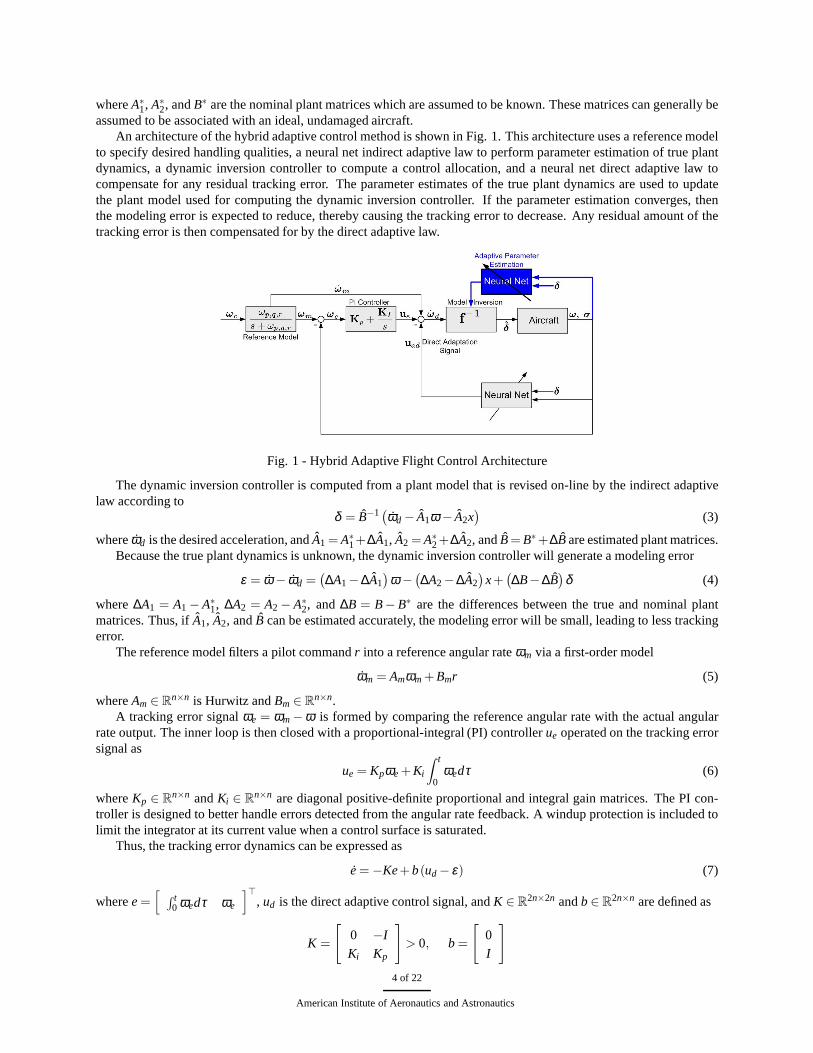
An architecture of the hybrid adaptive control method is shown in Fig. 1. This architecture uses a reference modelto specify desired handling qualities, a neural net indirect adaptive law to perform parameter estimation of true plantdynamics, a dynamic inversion controller to compute a control allocation, and a neural net direct adaptive law tocompensate for any residual tracking error. The parameter estimates of the true plant dynamics are used to updatethe plant model used for computing the dynamic inversion controller. If the parameter estimation converges, thenthe modeling error is expected to reduce, thereby causing the tracking error to decrease. Any residual amount of thetracking error is then compensated for by the direct adaptive law.

Fig. 1 - Hybrid Adaptive Flight Control Architecture

The dynamic inversion controller is computed from a plant model that is revised on-line by the indirect adaptivelaw according to

δ = B−1(ωd − A1ω − A2x)

(3)

whereωd is the desired acceleration, andA1 = A∗1+∆A1, A2 = A∗

2+∆A2, andB = B∗+∆B are estimated plant matrices.Because the true plant dynamics is unknown, the dynamic inversion controller will generate a modeling error

ε = ω − ωd =(

∆A1−∆A1)

ω −(

∆A2−∆A2)

x +(

∆B−∆B)

δ (4)

where∆A1 = A1 − A∗1, ∆A2 = A2 − A∗

2, and∆B = B− B∗ are the differences between the true and nominal plantmatrices. Thus, ifA1, A2, andB can be estimated accurately, the modeling error will be small, leading to less trackingerror.

The reference model filters a pilot commandr into a reference angular rateωm via a first-order model

ωm = Amωm + Bmr (5)

whereAm ∈ Rn×n is Hurwitz andBm ∈ R

n×n.A tracking error signalωe = ωm −ω is formed by comparing the reference angular rate with the actual angular

rate output. The inner loop is then closed with a proportional-integral (PI) controllerue operated on the tracking errorsignal as

ue = Kpωe + Ki

∫ t

0ωedτ (6)

whereKp ∈ Rn×n andKi ∈ R

n×n are diagonal positive-definite proportional and integral gain matrices. The PI con-troller is designed to better handle errors detected from the angular rate feedback. A windup protection is included tolimit the integrator at its current value when a control surface is saturated.

Thus, the tracking error dynamics can be expressed as

e = −Ke + b(ud − ε) (7)

wheree =[

∫ t0 ωedτ ωe

]>, ud is the direct adaptive control signal, andK ∈ R

2n×2n andb ∈ R2n×n are defined as

K =

[

0 −I

Ki Kp

]

> 0, b =

[

0

I

]

4 of 22


The eigenvalues ofK are found to be as

λ (K) = diag

Kp

2±

(

K2p

4−Ki

) 12

(8)

To achieve good loop gains, the integral gain should be set such that the real part of the minimum eigenvalue isgreatest. This requires

Ki ≥K2

p

4(9)

The system then has two complex poles in the open left halfs-plane.Referring to Eq. (7), if the direct adaptive control signalud or the parameter estimation from the indirect adaptive

law could perfectly cancel out the modeling errorε , then the tracking error would tend to zero asymptotically.Inpractice, there is always some residual modeling error in the adaptation, so asymptotic stability of the tracking erroris not guaranteed, but a weaker uniformly asymptotic stability could be achieved by a proper design of the direct andindirect adaptive laws.

A. Lyapunov-Based Indirect Adaptive Law

The cancellation of the modeling error is handled by the neural net indirect and direct adaptive control signals. Let

ud = W>d βd (10)

∆A1 = W>ω βω (11)

∆A2 = W>x βx (12)

∆B = W>δ βδ (13)

whereWd, Wω , Wx, andWδ are neural net weights,βd , βω , βx, andβδ are basis functions.A modified single-layer sigma-pi neural network is used to model nonlinear plant parameters according to

βd =[

C1 C2 C3 C4 C5 C6

]>

whereCi, i = 1, . . . ,6, are inputs to the neural network consisting of control commands, sensor feedback, and biasterms defined as

C1 = ρaV 2[

1 α β α2 β 2 αβ]

C2 = ρaV 2ω>[

1 α β]

C3 = ρaV 2δ>[

1 α β]

C4 = ω>[

p q r]

C5 = ω>[

u v w]

C6 =[

1 θ φ δT

]

whereα, β , θ , φ , u, v, w, V , ρa, δT are angle of attack, sideslip angle, pitch angle, bank angle, forward speed, lateralspeed, normal speed, absolute speed, atmospheric density,and engine throttle, respectively.

Specifically,C1 models the aerodynamic moments due to the angle of attacks and sideslip,C2 models the aero-dynamic moments due to the angular rate,C3 models the aerodynamic moments due to the flight control surface

5 of 22


deflections,C4 models the inertial moments, andC5 andC6 model the inertial moments due to the center-of-gravity(CG) shift. The basis functionsβω , βx, andβδ can be any suitable subset ofβd such as

βω = ρaV 2

1 α β1 α β1 α β

>

βx = ρaV 2

βδ = βω

The tracking error dynamics can now be written as

e = −Ke + bΦ>Θ + b(ud −∆ω) (14)

whereΦ> =[

W>ω W>

x W>δ

]

is a neural net weight matrix withΦ∈R(2n+m)×n andΘ> =

[

ω>β>ω x>β>

x δ>β>δ

]

is an input matrix withΘ ∈ R2n+m.

The neural net weightWd is computed by the direct adaptive law due to Rysdyk and Calise with a learning rateΓ > 0 and an e-modification parameterµ > 014 according to

Wd = −Γ(

βde>Pb + µ∥

∥

∥e>Pb∥

∥

∥Wd

)

(15)

where‖.‖ is a Frobenius norm andP ∈ R2n×2n solves the Lyapunov equation

K>P+ PK = Q (16)

for some positive-definite matrixQ.Let Q = I2n×2n, then solving forP in the Lyapunov equation yields

P =12

[

K−1i Kp + K−1

p (Ki + I) K−1i

K−1i K−1

p

(

I + K−1i

)

]

> 0

The e-modification term provides robustness in the direct adaptive law.14 The weight update law in Eq. (15)provides uniform boundedness of the neural net weight and the tracking error. The proof of this update law is providedby Rysdyk and Calise.5

The plant matrices∆A1, ∆A2, and∆B can be estimated using the Lyapunov direct method. The parameter estima-tion is given by the following normalized weight update law

Φ = −Λm2

(

Θe>Pb + η∥

∥

∥e>Pb∥

∥

∥Φ)

(17)

whereΛ > 0 is a learning rate,η ≥ 0 is an e-modification parameter, andm2 ∈ R is a normalization factor defined as

m = 1+ Θ>RΘ (18)

with R ∈ R(2n+m)×(2n+m) is a positive-semi-definite weight matrix. The normalization helps improve the adaptation

and prevent high-gain learning.The indirect adaptive law (17) is a stable adaptive law whichcan be proved as follows:Proof: Let Wd = W ∗

d +Wd andΦ = Φ∗ + Φ, where the asterisk denotes the ideal weight matrices and the tildedenotes the weight deviations. The ideal weight matrices are unknown but they may be assumed constant and boundedto stay within a∆e-neighborhood, where

∆e = supβd

∥

∥

∥W ∗>d βd + Φ∗>Θ−∆ω

∥

∥

∥

Consider the following Lyapunov candidate function

V = e>Pe + tr(

W>d Γ−1Wd + Φ>m2Λ−1Φ

)

6 of 22


where tr(.) is a matrix trace operator.The time derivative of the Lyapunov candidate function is then computed as

V ≤−e>Qe +2e>Pb(

W>d βd + Φ>Θ + ∆e

)

+2tr[

−W>d βde>Pb

− µW>d

∥

∥

∥e>Pb∥

∥

∥

(

W ∗d +Wd

)

− Φ>Θe>Pb− Φ>η∥

∥

∥e>Pb∥

∥

∥

(

Φ∗ + Φ)

]

Completing the square yields

tr[

−W>d µ∥

∥

∥e>Pb∥

∥

∥

(

W ∗d +Wd

)

]

= −∥

∥

∥e>Pb∥

∥

∥

∥

∥

∥

∥

µ12

(

W ∗d

2+Wd

)∥

∥

∥

∥

2

−

∥

∥

∥

∥

∥

µ12W ∗

d

2

∥

∥

∥

∥

∥

2

tr[

−Φ>η∥

∥

∥e>Pb∥

∥

∥

(

Φ∗ + Φ)

]

= −∥

∥

∥e>Pb∥

∥

∥

∥

∥

∥

∥

η12

(

Φ∗

2+ Φ

)∥

∥

∥

∥

2

−

∥

∥

∥

∥

∥

η12 Φ∗

2

∥

∥

∥

∥

∥

2

We then obtain

V ≤−e>Qe +2e>Pb∆e −2∥

∥

∥e>Pb∥

∥

∥

∥

∥

∥

∥

µ12

(

W ∗d

2+Wd

)∥

∥

∥

∥

2

−

∥

∥

∥

∥

∥

µ 12W ∗

d

2

∥

∥

∥

∥

∥

2

−2∥

∥

∥e>Pb∥

∥

∥

∥

∥

∥

∥

η12

(

Φ∗

2+ Φ

)∥

∥

∥

∥

2

−

∥

∥

∥

∥

∥

η12 Φ∗

2

∥

∥

∥

∥

∥

2

Since‖b‖ = 1, we establish thate>Qe ≤ ρ (Q)‖e‖2

e>Pb∆e ≤ ρ (P)‖e‖‖∆e‖

∥

∥

∥e>Pb∥

∥

∥

∥

∥

∥

∥

∥

µ12W ∗

d

2

∥

∥

∥

∥

∥

2

≤ ρ (P)‖e‖

∥

∥

∥

∥

∥

µ12W ∗

d

2

∥

∥

∥

∥

∥

2

∥

∥

∥e>Pb∥

∥

∥

∥

∥

∥

∥

∥

η 12 Φ∗

2

∥

∥

∥

∥

∥

2

≤ ρ (P)‖e‖

∥

∥

∥

∥

∥

η 12 Φ∗

2

∥

∥

∥

∥

∥

2

whereρ (P) andρ (P) are the spectral radii ofQ andP.Thus, the hybrid adaptive law is uniformly asymptotically stable provided that

‖e‖ >ρ (P)

2ρ (Q)

(

4‖∆e‖+∥

∥

∥µ12W ∗

d

∥

∥

∥

2+∥

∥

∥η12 Φ∗

∥

∥

∥

2)

We have ˙e, Θ/m ∈ L∞, bute ∈ L2 since

∫ ∞

0e>Qedt ≤ ρ (Q)

∫ ∞

0‖e‖2 dt ≤V (0)−V (t → ∞)+2ρ (P)

∫ ∞

0‖e‖‖∆e‖dt

−2ρ (P)∫ ∞

0‖e‖

∥

∥

∥

∥

µ12

(

W ∗d

2+Wd

)∥

∥

∥

∥

2

−

∥

∥

∥

∥

∥

µ12W ∗

d

2

∥

∥

∥

∥

∥

2

+

∥

∥

∥

∥

η12

(

Φ∗

2+ Φ

)∥

∥

∥

∥

2

−

∥

∥

∥

∥

∥

η12 Φ∗

2

∥

∥

∥

∥

∥

2

dt < ∞

This can be simplified as

V (t → ∞) ≤V (0)−2ρ (P)

∫ ∞

0‖e‖

(

∥

∥

∥

∥

µ12

(

W ∗d

2+Wd

)∥

∥

∥

∥

2

+

∥

∥

∥

∥

η12

(

Φ∗

2+ Φ

)∥

∥

∥

∥

2)

dt < ∞

7 of 22


Thus, the value ofV ast → ∞ and the tracking errore are uniformly bounded. Furthermore, if∆e = 0, µ = 0 andη = 0, we establish by means of the LaSalle-Yoshizawa theorem that limt→∞ ‖e‖→ 0 so that

∥

∥Wd

∥

∥→ 0 and∥

∥Φ∥

∥→ 0ast → ∞. This means that the indirect adaptive law will result in a convergence of the estimated∆A1, ∆A2, and∆B totheir steady state values if there is no neural network approximation error and the input signals are sufficiently rich toexcite all frequencies of interest in the plant dynamics. This condition is known as a persistent excitation (PE)15

We note that the effect of the e-modificationµ andη parameters is to increase the negative time rate of changeof the Lyapunov candidate function so that as long as the effects of unmodeled dynamics and or disturbances do notexceed the value ofV (0), the adaptive signals should remain bounded. The e-modification thus makes the adaptivelaw robust to unmodeled dynamics.16 However, this usually comes at a sacrifice in performance as will be shown later.

�

B. Recursive Least-Squares Indirect Adaptive Law

A recursive least-squares (RLS) method can be used in lieu ofthe normalized Lyapunov-based indirect adaptive law(17) for identifying plant dynamics. The RLS method is an adaptive law based on the optimal estimation method thatuses the modeling error as the adaptive signal instead of thetracking error as in the Lyapunov-based indirect adaptivelaw. The plant matrices∆A1, ∆A2, and∆B can be estimated as

∆A1 = W>ω βω (19)

∆A2 = W>x βx (20)

∆B = W>δ βδ (21)

with the following weight update law

Φ = −1m

RΘ(

Θ>Φ− ε∗>)

(22)

R = −1m

RΘΘ>R (23)

whereε∗ε∗ = ˙ω −A∗

1ω −A∗2x−B∗δ (24)

is the estimated modeling error for a fixed nominal plant model which requires an estimated angular acceleration˙ωas an input. Generally, the angular acceleration may not be available rate gyro sensors, but can be estimated from aKalman filter, a differentiator, or a numerical filter via a cubic or B-spline method. In any case, the estimation of theangular acceleration will introduce an error source. If theerror is unbiased, i.e., it can be characterized as a white noiseabout the mean value, then the RLS indirect adaptive law can be applied to estimate the changes in the plant dynamics.

The tracking error dynamics for the RLS indirect adaptive law are expressed as

e = −Ke + bud + b(

Φ>Θ− ε∗)

(25)

The proof of the RLS indirect adaptive law is as follows:Proof:To reduce the tracking error, the modeling error must be keptminimum. The optimal estimation method

can be used to minimize the modeling error. Consider the following cost least-squares functional

J (Φ) =12

∫ t

0

1m2

∥

∥

∥Φ>Θ− ε∗∥

∥

∥

2dτ

To minimize the cost functional, we compute its gradient with respect toΦ and set it to zero, thus resulting in

∇J>Φ =

∫ t

0

1m2 Θ

(

Θ>Φ− ε∗>)

dτ = 0

This can be written as∫ t

0

1m2 ΘΘ>dτΦ =

∫ t

0

1m2 Θε∗>dτ

8 of 22


Let

R−1 =

∫ t

0

1m2 ΘΘ>dτ

Then

R−1Φ =

∫ t

0

1m2 Θε∗>dτ

Upon differentiation

R−1Φ+1

m2 ΘΘ>Φ =1

m2 Θε∗>

and solving forΦ, the RLS indirect adaptive law is obtained as

Φ = −1

m2 RΘ(

Θ>Φ− ε∗>)

Also, we note thatR−1R = I ⇒ R−1R + R−1R = 0

Solving forR yields

R = −RR−1R = −1

m2 RΘΘ>R

The RLS formula has a very similar form to the Kalman filter where Eq. (23) is a differential Riccati equation for azero-order plant dynamics andR is called a covariance matrix. In the RLS indirect adaptive law,R acts as an adaptivelearning rate with its own update law. With large enoughR, the ideal productΦ∗>Θ can be shown to converge to theestimated modeling errorε∗15 so that

∥

∥

∥Φ∗>Θ− ε∗

∥

∥

∥< M

whereM > 0 is some small positive constant. Then, the time derivativeof the weight variationΦ is equal to

˙Φ = −1

m2 RΘΘ>Φ

The RLS indirect adaptive law can now be shown to be stable andresult in bounded signals. Consider the followingLyapunov candidate function

V = e>Pe + tr(

W>d Γ−1Wd + Φ>R−1Φ

)

The time rate of change of the Lyapunov candidate function iscomputed as

V ≤−e>Qe +2e>Pb(

W>d βd + Φ>Θ + ∆e

)

+2tr

[

−W>d βde>Pb− µW>

d

∥

∥

∥e>Pb∥

∥

∥

(

W ∗d +Wd

)

−1

m2 Φ>ΘΘ>Φ]

where∆e = sup

βd

∥

∥

∥W ∗>d βd + M

∥

∥

∥

We note that now the neural net direct adaptive law only needsto cancel out the residual recursive least-squareserror which should be small enough that the learning rate does not have to be set to a large value, thereby reducing theeffect of high-gain learning

Upon simplification, one obtains

V ≤−e>Qe−2∥

∥

∥e>Pb∥

∥

∥

∥

∥

∥

∥

µ12

(

W ∗d

2+Wd

)∥

∥

∥

∥

2

−2tr

(

1m2 Φ>ΘΘ>Φ

)

≤ 0

Thus, the hybrid adaptive law with the recursive least-squares indirect adaptive law is stable provided that thetracking error is bounded from below by

infβd

‖e‖ =ρ (P)‖∆e‖

2ρ (Q)

(

4‖∆e‖+∥

∥

∥µ12W ∗

d

∥

∥

∥

2)

�

9 of 22


III. Bounded Linear Stability Analysis

A key challenge with neural net adaptive flight control is to make the learning algorithm sufficiently robust. Ro-bustness relates to the stability and convergence of the learning algorithm. Stability is a fundamental requirement ofany dynamical system that ensures a small disturbance wouldnot grow to a large deviation from an equilibrium. Forsystems with high assurance such as human-rated or mission-critical flight vehicles, stability of adaptive systems is ofparamount importance. Without guaranteed stability, suchadaptive control algorithms cannot be certified for opera-tion in high-assurance systems. Unfortunately, the stability of adaptive controllers in general and neural net adaptivecontrollers in particular remains unresolved. The notion of a self-modifying flight control law using an artificial neuralnet learning process whose outputs may be deemed as non-deterministic is a major huddle to overcome.

Another criterion for robustness is the convergence of the neural net learning algorithm. Neural networks are usedas universal nonlinear function approximators. In the caseof the adaptive flight control, the networks approximatethe unknown modeling error that is used to adjust effectively the control gains to maintain a desired handling quality.Convergence requires stability and a proper design of the weight update law. It is conceivable that even though alearning algorithm is stable, the neural net weights may notconverge to correct values. Thus, accurate convergence isalso important since this is directly related to the flight control performance.

The neural net weight update laws in Eqs. (15), (17), and (22)are nonlinear due to the product terms involvingβd , e, Φ, andΘ. Stability of nonlinear systems is usually analyzed by the Lyapunov method. However, the concept ofphase and gain margin for linear systems cannot be extended to nonlinear adaptive control. The linear control marginconcept can provide understanding stability margin of adaptive control that enables more robust adaptive learning lawsto be synthesized. This is only possible if the neural net weight update laws are linearized at a certain point in timewith the neural net weights held constant. As adaptation occurs, the neural net weights vary with time. Hence, thetime at which to freeze the neural net weights (for calculation) must correspond to a worst-case stability margin. Thiscan be a challenge. This paper introduces a method for analyzing stability and convergence of nonlinear neural netadaptive laws using error bound analysis, which enables thedominant linear components of the nonlinear adaptivelaws to be extracted from Eqs. (15), (17), and (22) without linearization of the adaptive laws at an instance in time.

A. Lyapunov-Based Direct Adaptive Law

For the direct adaptive law in Eq. (15), we note that it can be expressed as

ddt

(

β>d Wd

)

= −Γ(

β>d βde>Pb + µ

∥

∥

∥e>Pb

∥

∥

∥β>

d Wd

)

+ β>d Wd (26)

We define an error bound on the neural net adaptive signal as

∆Wd= sup

βd

∥

∥

∥W>d βd −Γµ

∥

∥

∥e>Pb∥

∥

∥W ∗>d β

∥

∥

∥ (27)

Then, the time derivative of the variation in the neural net direct adaptive signal is bounded by

ddt

(

W>d βd

)

≤−Γ(

α0β>d Pe + µγW>

d βd

)

+ ∆Wd(28)

whereγ = sup

ω

∥

∥

∥e>Pb∥

∥

∥ (29)

andα0 > 0 is defined as a level of persistent excitation (PE) such thatthe followingL2-norm PE condition is satisfied

∥

∥

∥β>d βd

∥

∥

∥=1T

∫ t+T

tβ>

d βddτ ≤ α0 (30)

for β ∈ L2.Thus, without sufficient persistent excitation and if the e-modification parameterµ is not present, the neural net

weights will not necessarily converge. The persistent excitation essentially means that inputs to the neural networkmust be sufficiently rich in order to excite system dynamics to enable a convergence to take place.

10 of 22


If the error bound is small, then the linear behavior of the weight update law becomes dominant. Therefore, thisenables the stability and convergence to be analyzed in a linear sense using the following equation

ddt

[

e

W>d βd

]

≤

[

−K b

−Γα0b>P −Γµγ

][

e

W>d βd

]

+

[

∆e

∆Wd

]

(31)

LetA be the transition matrix. IfA is negative definite, then the rate of convergence is established by the eigenvaluesof A since

[

e

W>d βd

]

≤ eAt

[

e(0)

W>d (0)βd (0)

]

−A−1

[

∆e

∆Wd

]

(32)

The equilibrium is therefore uniformly asymptotically stable and converges to

limt→∞

supβd

∥

∥

∥

∥

∥

e

W>d βd

∥

∥

∥

∥

∥

=

∥

∥

∥

∥

∥

A−1

[

∆e

∆Wd

]∥

∥

∥

∥

∥

(33)

By Holder’s inequality, the convergence radius can be expressed as

limt→∞

supβd

∥

∥

∥

∥

∥

e

W>d βd

∥

∥

∥

∥

∥

≤ ρ(

A−1)∥

∥

∥

∥

∥

∆e

∆Wd

∥

∥

∥

∥

∥

(34)

Thus, ∆e and∆Wdshould be kept as small as possible for the tracking error andthe neural net weight matrix

variation to converge as close to zero as possible.In order to obtain a convergence, stability of the tracking error and neural net adaptive law must be established by

the negative-definiteness of the eigenvalues ofA. The characteristic equation of A is established by det(sI −A), whichcan be computed using the Schur complement

det(sI −A) = (s+ Γµγ)det[

sI + K + b(s+ Γµγ)−1 Γα0b>P]

(35)

Upon expansion, the characteristic equation is obtained as

s3 + Kps2 + Kis+ Γ[

µγs2 +(µγKp + α0P22) s+ µγKi + α0P12]

= 0 (36)

This equation represents the characteristic equation of the following open-loop transfer function

H (s) = (sI + K)−1C (s) (37)

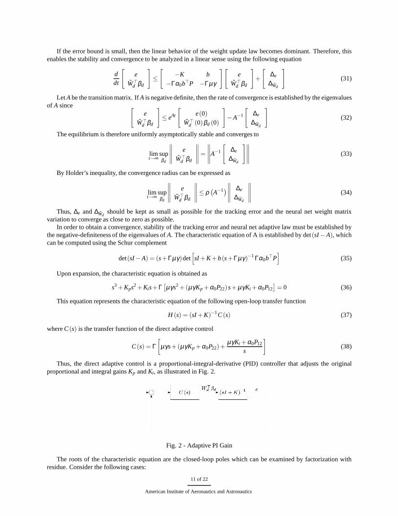
whereC (s) is the transfer function of the direct adaptive control

C (s) = Γ[

µγs+(µγKp + α0P22)+µγKi + α0P12

s

]

(38)

Thus, the direct adaptive control is a proportional-integral-derivative (PID) controller that adjusts the originalproportional and integral gainsKp andKi, as illustrated in Fig. 2.

Fig. 2 - Adaptive PI Gain

The roots of the characteristic equation are the closed-loop poles which can be examined by factorization withresidue. Consider the following cases:

11 of 22


1. If µ is small andµ � min

(

α0K−1p P22γ ,

α0K−1i P12γ

)

, then Eq. (36) can be factored as

(s+ Γa)[

s2 +(Kp + Γµγ −Γa)s+ Ki + ΓµγKp + Γα0P22−Γa(Kp + Γµγ −Γa)]

+ r = 0 (39)

wherea and the residuer are defined as

a = (Ki + ΓµγKp + Γα0P22)−1(µγKi + α0P12) (40)

r = Γ(µγKi + α0P12)−Γa [Ki + Γ(µγKp + α0P22)−Γa(Kp + Γµγ −Γa)] (41)

Consider two cases:

(a) For smallΓ, which corresponds to slow adaptation, we see that

a ≈ µγ + α0K−1i P12 (42)

r ≈ 0 (43)

Neglecting second-order terms ofΓ, The approximate roots of the characteristic equation are then foundto be

s ≈−Kp −Γα0K−1

i P12

2± j

[

Ki + Γα0(

P22−K−1i P12Kp

)

−

(

Kp −Γα0K−1i P12

)2

4

]

12

(44)

s ≈−Γ(

µγ + α0K−1i P12

)

(45)

From the complex-valued roots, the effect of the direct adaptive control is to adjust the PI gains accordingto

Kp = Kp −Γα0K−1i P12 (46)

Ki = Ki + Γα0(

P22−K−1i P12Kp

)

(47)

where the bar denotes the adaptive PI gains.The convergence radius for slow adaptation is then equal to

limt→∞

supβd

∥

∥

∥

∥

∥

e

W>d βd

∥

∥

∥

∥

∥

≤

(

µγ + α0K−1i P12

)−1

Γ

∥

∥

∥

∥

∥

∆e

∆Wd

∥

∥

∥

∥

∥

(48)

Thus, slow adaptation results in a large convergence radiussinceΓ is small.

(b) For largeΓ, which corresponds to fast adaptation or high-gain learning, we see that

Γa ≈−P−122 P12 (49)

r ≈−Γa [Ki −Γa(Kp + Γµγ −Γa)] (50)

Sinceµ is small andΓa is finitely small even thoughΓ is large, then the residuer is also finitely smallcompared tos which is large. The approximate roots of the characteristicequation are obtained as

s ≈−Kp + Γµγ −P−1

22 P12

2± j

{

Ki + Γ[

α0P22+ µγ(

Kp −P−122 P12

)]

−

(

Kp + Γµγ −P−122 P12

)2

4

}

(51)

s ≈−P−122 P12 (52)

The adaptive PI gains according toKp = Kp + Γµγ −P−1

22 P12 (53)

Ki = Ki + Γ[

α0P22− µγ(

Kp −P−122 P12

)]

(54)

12 of 22


The convergence radius for high-gain learning is equal to

limt→∞

supβd

∥

∥

∥

∥

∥

e

W>d βd

∥

∥

∥

∥

∥

≤ P−112 P22

∥

∥

∥

∥

∥

∆e

∆Wd

∥

∥

∥

∥

∥

(55)

The effect of high-learning can be discerned from the adaptive PI gains. Increasing learning causes boththe Kp andKi gain to increase accordingly. The highKi gain will result in a high frequency oscillationin the adaptive signal.9 This high frequency oscillation can result in excitation ofunmodeled dynamicsthat may be present in the system and therefore can lead to a possibility of instability since the effects ofunmodeled dynamics are not accounted in the Lyapunov analysis of the neural net weight update law.15

2. If µ is sufficiently large and andµ �max

(

α0K−1p P22γ ,

α0K−1i P12γ

)

, then the characteristic equation can be reduced

tos3 + Kps2 + Kis+ Γµγ

(

s2 + Kps+ Ki)

= 0 (56)

The roots are found to be

s = −Kp

2± j

(

Ki −K2

p

4

) 12

(57)

s = −Γµγ (58)

The complex conjugate roots reveal that for a sufficiently large µ , the effect of learning is zero because the PIgains are reduced to their original value. Thus, increasingµ beyond a certain value can negate the potentialbenefits due to adaptive control. This can also be seen from the transfer functionC (s) whereµ is the derivativegain which tends to increase damping of the tracking error response.

The convergence radius for slow adaptation is equal to

limt→∞

supβd

∥

∥

∥

∥

∥

e

W>d βd

∥

∥

∥

∥

∥

≤1

Γµγ

∥

∥

∥

∥

∥

∆e

∆Wd

∥

∥

∥

∥

∥

(59)

The convergence radius for fast adaptation is equal to

limt→∞

supβd

∥

∥

∥

∥

∥

e

W>d βd

∥

∥

∥

∥

∥

≤ K−1i

∥

∥

∥

∥

∥

∆e

∆Wd

∥

∥

∥

∥

∥

(60)

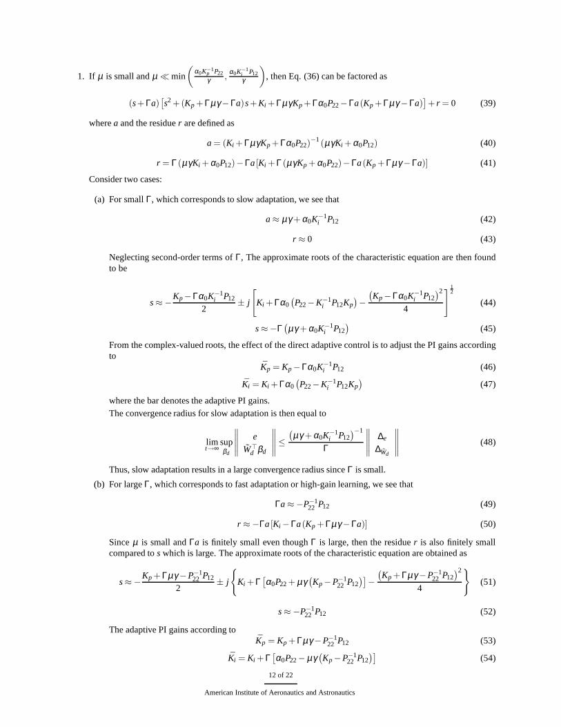
To illustrate the bounded linear stability analysis, a simulation was performed for a damaged twin-engine generictransport model (GTM),22 as shown in Fig. 3. A wing damage simulation was performed with 25% of the left wingmissing. The neural net direct adaptive control is implemented to maintain tracking performance of the damagedaircraft. A pitch doublet maneuver is commanded while the roll and yaw rates are regulated.

Fig. 3 - Generic Transport Model

13 of 22


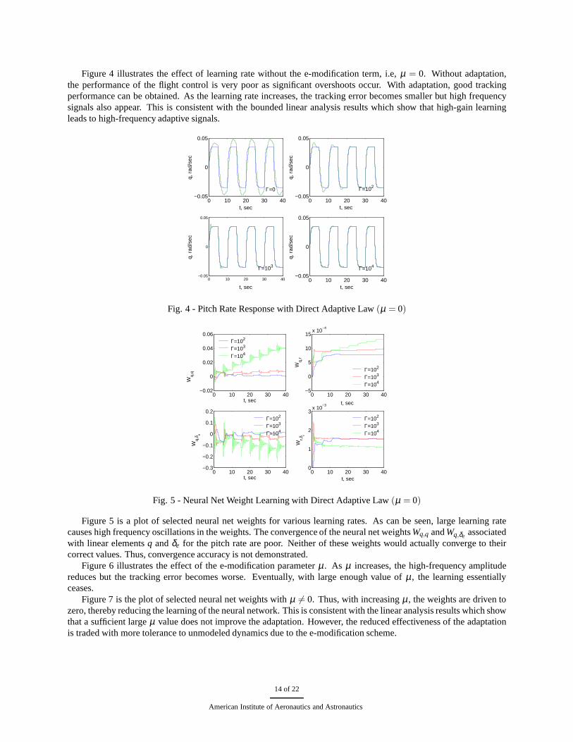
Figure 4 illustrates the effect of learning rate without thee-modification term, i.e,µ = 0. Without adaptation,the performance of the flight control is very poor as significant overshoots occur. With adaptation, good trackingperformance can be obtained. As the learning rate increases, the tracking error becomes smaller but high frequencysignals also appear. This is consistent with the bounded linear analysis results which show that high-gain learningleads to high-frequency adaptive signals.

0 10 20 30 40−0.05

0

0.05

t, sec

q, r

ad/s

ec

0 10 20 30 40−0.05

0

0.05

t, sec

q, r

ad/s

ec

0 10 20 30 40−0.05

0

0.05

t, sec

q, r

ad/s

ec

0 10 20 30 40−0.05

0

0.05

t, secq,

rad

/sec

Γ=0 Γ=102

Γ=103 Γ=104

Fig. 4 - Pitch Rate Response with Direct Adaptive Law(µ = 0)

0 10 20 30 400

1

2

3x 10

−3

t, sec

Wr,δ

r

0 10 20 30 40−0.3

−0.2

−0.1

0

0.1

0.2

Wq,

δ e

t, sec

0 10 20 30 40−0.02

0

0.02

0.04

0.06

Wq,

q

t, sec0 10 20 30 40

−5

0

5

10

15x 10

−4

Wq,

r

t, sec

Γ=102

Γ=103

Γ=104

Γ=102

Γ=103

Γ=104

Γ=102

Γ=103

Γ=104

Γ=102

Γ=103

Γ=104

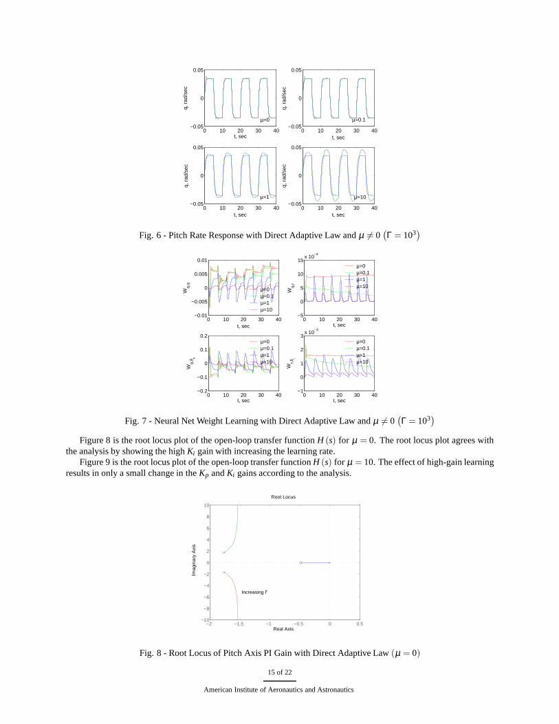
Fig. 5 - Neural Net Weight Learning with Direct Adaptive Law(µ = 0)

Figure 5 is a plot of selected neural net weights for various learning rates. As can be seen, large learning ratecauses high frequency oscillations in the weights. The convergence of the neural net weightsWq,q andWq,δe associatedwith linear elementsq andδe for the pitch rate are poor. Neither of these weights would actually converge to theircorrect values. Thus, convergence accuracy is not demonstrated.

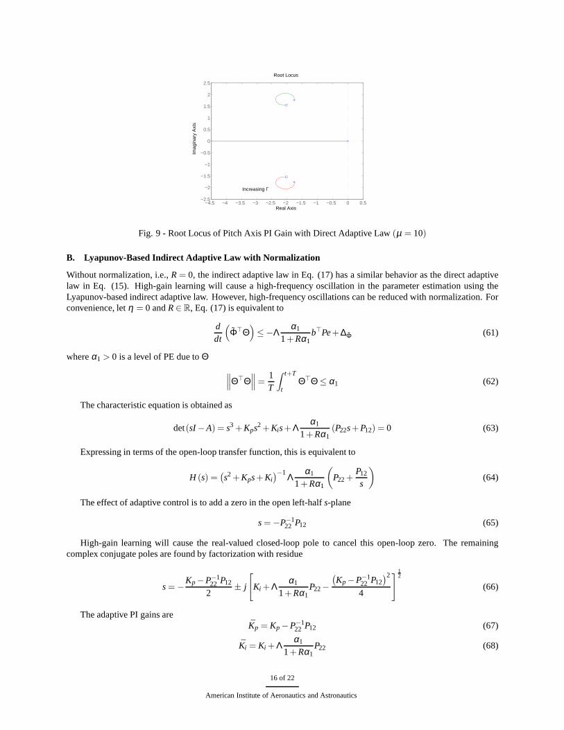
Figure 6 illustrates the effect of the e-modification parameter µ . As µ increases, the high-frequency amplitudereduces but the tracking error becomes worse. Eventually, with large enough value ofµ , the learning essentiallyceases.

Figure 7 is the plot of selected neural net weights withµ 6= 0. Thus, with increasingµ , the weights are driven tozero, thereby reducing the learning of the neural network. This is consistent with the linear analysis results which showthat a sufficient largeµ value does not improve the adaptation. However, the reducedeffectiveness of the adaptationis traded with more tolerance to unmodeled dynamics due to the e-modification scheme.

14 of 22


0 10 20 30 40−0.05

0

0.05

t, sec

q, r

ad/s

ec

0 10 20 30 40−0.05

0

0.05

t, sec

q, r

ad/s

ec

0 10 20 30 40−0.05

0

0.05

t, sec

q, r

ad/s

ec

0 10 20 30 40−0.05

0

0.05

t, sec

q, r

ad/s

ec

µ=0 µ=0.1

µ=1 µ=10

Fig. 6 - Pitch Rate Response with Direct Adaptive Law andµ 6= 0(

Γ = 103)

0 10 20 30 40−0.01

−0.005

0

0.005

0.01

t, sec

Wq,

q

0 10 20 30 40−5

0

5

10

15x 10

−4

Wq,

r

t, sec

0 10 20 30 40−0.2

−0.1

0

0.1

0.2

t, sec

Wq,

δ e

0 10 20 30 40−1

0

1

2

3x 10

−3

t, sec

Wr,δ

rµ=0µ=0.1µ=1µ=10

µ=0µ=0.1µ=1µ=10

µ=0µ=0.1µ=1µ=10

µ=0µ=0.1µ=1µ=10

Fig. 7 - Neural Net Weight Learning with Direct Adaptive Law and µ 6= 0(

Γ = 103)

Figure 8 is the root locus plot of the open-loop transfer function H (s) for µ = 0. The root locus plot agrees withthe analysis by showing the highKi gain with increasing the learning rate.

Figure 9 is the root locus plot of the open-loop transfer function H (s) for µ = 10. The effect of high-gain learningresults in only a small change in theKp andKi gains according to the analysis.

−2 −1.5 −1 −0.5 0 0.5−10

−8

−6

−4

−2

0

2

4

6

8

10

Root Locus

Real Axis

Imag

inar

y A

xis

Increasing Γ

Fig. 8 - Root Locus of Pitch Axis PI Gain with Direct Adaptive Law (µ = 0)

15 of 22


−4.5 −4 −3.5 −3 −2.5 −2 −1.5 −1 −0.5 0 0.5−2.5

−2

−1.5

−1

−0.5

0

0.5

1

1.5

2

2.5

Root Locus

Real Axis

Imag

inar

y A

xis

Increasing Γ

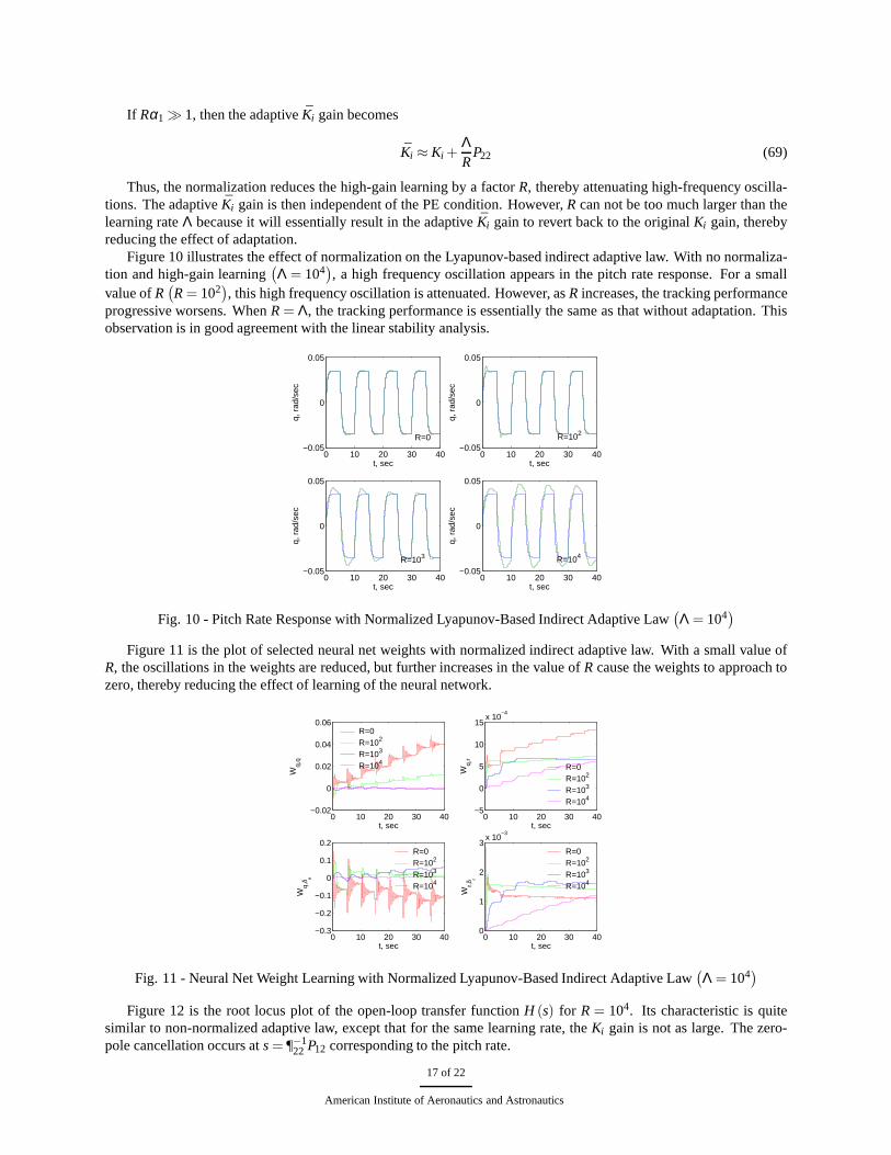
Fig. 9 - Root Locus of Pitch Axis PI Gain with Direct Adaptive Law (µ = 10)

B. Lyapunov-Based Indirect Adaptive Law with Normalization

Without normalization, i.e.,R = 0, the indirect adaptive law in Eq. (17) has a similar behavior as the direct adaptivelaw in Eq. (15). High-gain learning will cause a high-frequency oscillation in the parameter estimation using theLyapunov-based indirect adaptive law. However, high-frequency oscillations can be reduced with normalization. Forconvenience, letη = 0 andR ∈ R, Eq. (17) is equivalent to

ddt

(

Φ>Θ)

≤−Λα1

1+ Rα1b>Pe + ∆Φ (61)

whereα1 > 0 is a level of PE due toΘ∥

∥

∥Θ>Θ∥

∥

∥=1T

∫ t+T

tΘ>Θ ≤ α1 (62)

The characteristic equation is obtained as

det(sI −A) = s3 + Kps2 + Kis+ Λα1

1+ Rα1(P22s+ P12) = 0 (63)

Expressing in terms of the open-loop transfer function, this is equivalent to

H (s) =(

s2 + Kps+ Ki)−1 Λ

α1

1+ Rα1

(

P22+P12

s

)

(64)

The effect of adaptive control is to add a zero in the open left-half s-plane

s = −P−122 P12 (65)

High-gain learning will cause the real-valued closed-looppole to cancel this open-loop zero. The remainingcomplex conjugate poles are found by factorization with residue

s = −Kp −P−1

22 P12

2± j

[

Ki + Λα1

1+ Rα1P22−

(

Kp −P−122 P12

)2

4

]

12

(66)

The adaptive PI gains areKp = Kp −P−1

22 P12 (67)

Ki = Ki + Λα1

1+ Rα1P22 (68)

16 of 22


If Rα1 � 1, then the adaptiveKi gain becomes

Ki ≈ Ki +ΛR

P22 (69)

Thus, the normalization reduces the high-gain learning by afactorR, thereby attenuating high-frequency oscilla-tions. The adaptiveKi gain is then independent of the PE condition. However,R can not be too much larger than thelearning rateΛ because it will essentially result in the adaptiveKi gain to revert back to the originalKi gain, therebyreducing the effect of adaptation.

Figure 10 illustrates the effect of normalization on the Lyapunov-based indirect adaptive law. With no normaliza-tion and high-gain learning

(

Λ = 104)

, a high frequency oscillation appears in the pitch rate response. For a smallvalue ofR

(

R = 102)

, this high frequency oscillation is attenuated. However, asR increases, the tracking performanceprogressive worsens. WhenR = Λ, the tracking performance is essentially the same as that without adaptation. Thisobservation is in good agreement with the linear stability analysis.

0 10 20 30 40−0.05

0

0.05

t, secq,

rad

/sec

0 10 20 30 40−0.05

0

0.05

t, sec

q, r

ad/s

ec

0 10 20 30 40−0.05

0

0.05

t, sec

q, r

ad/s

ec0 10 20 30 40

−0.05

0

0.05

t, sec

q, r

ad/s

ec

R=102 R=0

R=103 R=104

Fig. 10 - Pitch Rate Response with Normalized Lyapunov-Based Indirect Adaptive Law(

Λ = 104)

Figure 11 is the plot of selected neural net weights with normalized indirect adaptive law. With a small value ofR, the oscillations in the weights are reduced, but further increases in the value ofR cause the weights to approach tozero, thereby reducing the effect of learning of the neural network.

0 10 20 30 40−0.02

0

0.02

0.04

0.06

t, sec

Wq,

q

0 10 20 30 40−5

0

5

10

15x 10

−4

t, sec

Wq,

r

0 10 20 30 40−0.3

−0.2

−0.1

0

0.1

0.2

t, sec

Wq,

δ e

0 10 20 30 400

1

2

3x 10

−3

t, sec

Wr,δ

r

R=0R=102

R=103

R=104

R=0R=102

R=103

R=104

R=0R=102

R=103

R=104

R=0R=102

R=103

R=104

Fig. 11 - Neural Net Weight Learning with Normalized Lyapunov-Based Indirect Adaptive Law(

Λ = 104)

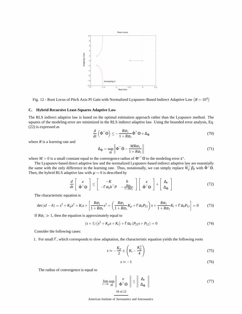
Figure 12 is the root locus plot of the open-loop transfer function H (s) for R = 104. Its characteristic is quitesimilar to non-normalized adaptive law, except that for thesame learning rate, theKi gain is not as large. The zero-pole cancellation occurs ats = ¶−1

22 P12 corresponding to the pitch rate.

17 of 22


−2 −1.5 −1 −0.5 0 0.5−10

−8

−6

−4

−2

0

2

4

6

8

10

Root Locus

Real Axis

Imag

inar

y A

xis

Increasing Λ

Fig. 12 - Root Locus of Pitch Axis PI Gain with Normalized Lyapunov-Based Indirect Adaptive Law(

R = 104)

C. Hybrid Recursive Least-Squares Adaptive Law

The RLS indirect adaptive law is based on the optimal estimation approach rather than the Lyapunov method. Thesquares of the modeling error are minimized in the RLS indirect adaptive law. Using the bounded error analysis, Eq.(22) is expressed as

ddt

(

Φ>Θ)

≤−Rα1

1+ Rα1Φ>Θ + ∆Φ (70)

whereR is a learning rate and

∆Φ = supΘ

∥

∥

∥

∥

Φ>Θ−MRα1

1+ Rα1

∥

∥

∥

∥

(71)

whereM > 0 is a small constant equal to the convergence radius ofΦ∗>Θ to the modeling errorε∗.The Lyapunov-based direct adaptive law and the normalized Lyapunov-based indirect adaptive law are essentially

the same with the only difference in the learning rate. Thus,notationally, we can simply replaceW>d βd with Φ>Θ.

Then, the hybrid RLS adaptive law withµ = 0 is described by

ddt

[

e

Φ>Θ

]

≤

[

−K b

−Γα0b>P − Rα11+Rα1

][

e

Φ>Θ

]

+

[

∆e

∆Φ

]

(72)

The characteristic equation is

det(sI−A) = s3 + Kps2 + Kis+

[

Rα1

1+ Rα1s2 +

(

Rα1

1+ Rα1Kp + Γα0P22

)

s+Rα1

1+ Rα1Ki + Γα0P12

]

= 0 (73)

If Rα1 � 1, then the equation is approximately equal to

(s+1)(

s2 + Kps+ Ki)

+ Γα0 (P22s+ P12) = 0 (74)

Consider the following cases:

1. For smallΓ, which corresponds to slow adaptation, the characteristicequation yields the following roots

s ≈−Kp

2±

(

Ki −K2

p

4

)

(75)

s ≈−1 (76)

The radius of convergence is equal to

limt→∞

supΘ

∥

∥

∥

∥

∥

e

Φ>Θ

∥

∥

∥

∥

∥

≤

∥

∥

∥

∥

∥

∆e

∆Φ

∥

∥

∥

∥

∥

(77)

18 of 22


An interesting observation is made concerning the radius ofconvergence. Comparing with Eq. (48), the radiusof convergence for the hybrid RLS adaptive law is independent of the learning rate. So, for a small learning rate,the radius of convergence for the Lyapunov-based direct adaptive law is large, but for the hybrid RLS adaptivelaw, it is finitely small. Moreover, the error bounds are not necessarily small for the Lyapunov-based directadaptive law if convergence accuracy is not achieved. On theother hand, the RLS indirect adaptive law can beshown to provide good convergence accuracy. Therefore, theradius of convergence for the hybrid RLS adaptivelaw is expected to be smaller for the same small learning rate. This would mean that the Lyapunov-based directadaptive law does not have to be a high-gain controller.

2. For largeΓ, which corresponds to high-gain learning, the characteristic equation can be factored as

(s+ Γa)[

s2 +(Kp +1−Γa)s+ Ki + Kp + Γα0P22−Γa(Kp +1−Γa)]

+ r = 0 (78)

where for largeΓΓa = P−1

22 P12 (79)

r = Ki − (Ki + Kp)P−122 P12+

(

P−122 P12

)2(Kp +1−P−1

22 P12)

(80)

For large learning rate,r is finitely smaller thans, so the approximate roots are

s = −Kp +1−P−1

22 P12

2± j

{

Ki + Kp −P−122 P12

(

Kp +1−P−122 P12

)

+ Γα0P22−

(

Kp +1−P−122 P12

)2

4

}

12

(81)

s = −P−122 P12 (82)

The adaptive gains areKp = Kp +1−P−1

22 P12 (83)

Ki = Ki + Kp −P−122 P12

(

Kp +1−P−122 P12

)

+ Γα0P22 (84)

On initial observation, we would see that high-gain learning would result in high-frequency oscillations as isthe case with the Lyapunov-based direct adaptive law. However, if the convergence of the parameter estimationis achieved with the RLS indirect adaptive law, the parameter estimates then result in a dynamic inversioncontroller that is better matched with the true plant dynamics so that the tracking error would be nearly zero.Consequently, the resulting direct adaptive signal would be very small so that even with high-gain learning, thehigh adaptiveKi gain would not inject high-frequency amplitude in the tracking error.

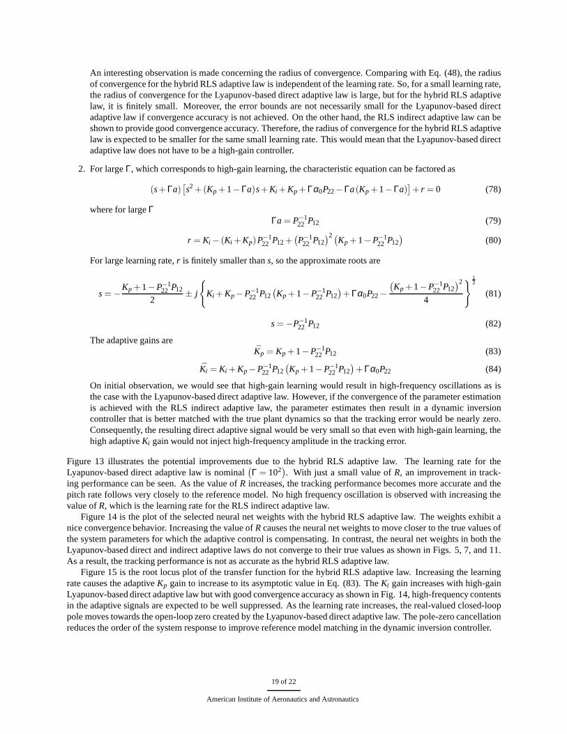
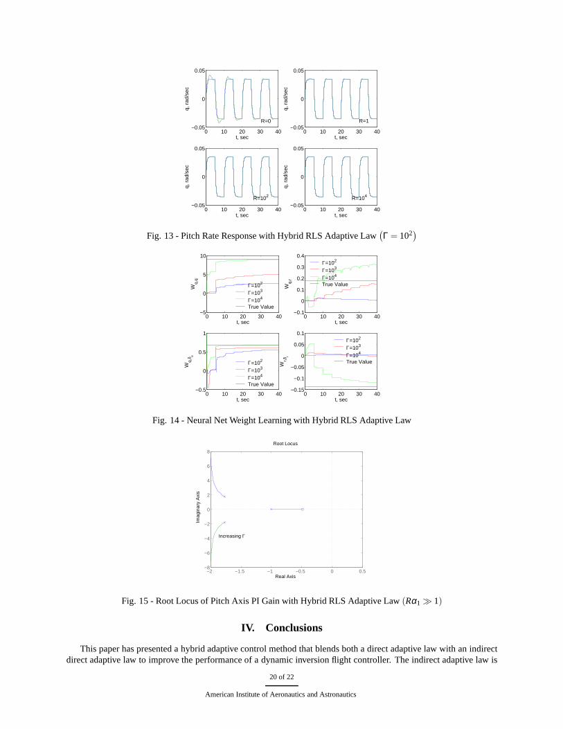
Figure 13 illustrates the potential improvements due to thehybrid RLS adaptive law. The learning rate for theLyapunov-based direct adaptive law is nominal

(

Γ = 102)

. With just a small value ofR, an improvement in track-ing performance can be seen. As the value ofR increases, the tracking performance becomes more accurateand thepitch rate follows very closely to the reference model. No high frequency oscillation is observed with increasing thevalue ofR, which is the learning rate for the RLS indirect adaptive law.

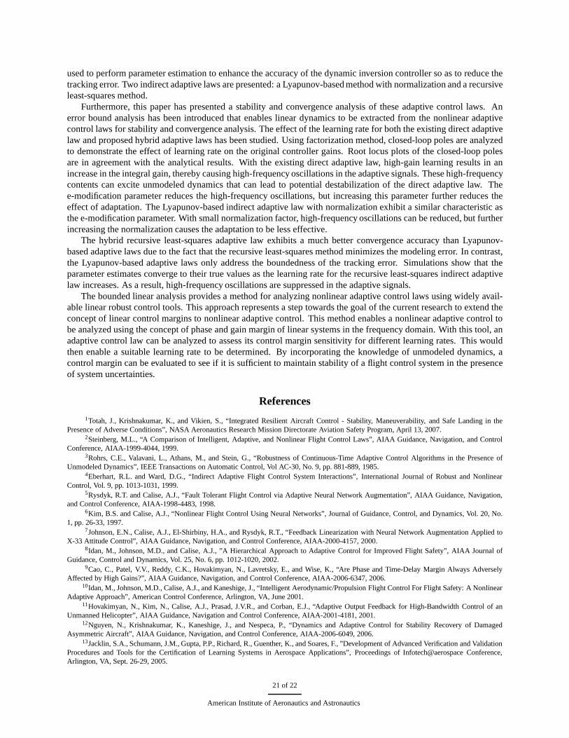
Figure 14 is the plot of the selected neural net weights with the hybrid RLS adaptive law. The weights exhibit anice convergence behavior. Increasing the value ofR causes the neural net weights to move closer to the true values ofthe system parameters for which the adaptive control is compensating. In contrast, the neural net weights in both theLyapunov-based direct and indirect adaptive laws do not converge to their true values as shown in Figs. 5, 7, and 11.As a result, the tracking performance is not as accurate as the hybrid RLS adaptive law.

Figure 15 is the root locus plot of the transfer function for the hybrid RLS adaptive law. Increasing the learningrate causes the adaptiveKp gain to increase to its asymptotic value in Eq. (83). TheKi gain increases with high-gainLyapunov-based direct adaptive law but with good convergence accuracy as shown in Fig. 14, high-frequency contentsin the adaptive signals are expected to be well suppressed. As the learning rate increases, the real-valued closed-looppole moves towards the open-loop zero created by the Lyapunov-based direct adaptive law. The pole-zero cancellationreduces the order of the system response to improve reference model matching in the dynamic inversion controller.

19 of 22


0 10 20 30 40−0.05

0

0.05

t, sec

q, r

ad/s

ec

0 10 20 30 40−0.05

0

0.05

t, sec

q, r

ad/s

ec

0 10 20 30 40−0.05

0

0.05

t, sec

q, r

ad/s

ec

0 10 20 30 40−0.05

0

0.05

t, sec

q, r

ad/s

ec

R=0 R=1

R=102 R=104

Fig. 13 - Pitch Rate Response with Hybrid RLS Adaptive Law(

Γ = 102)

0 10 20 30 40−5

0

5

10

Wq,

q

t, sec0 10 20 30 40

−0.1

0

0.1

0.2

0.3

0.4

Wq,

r

t, sec

0 10 20 30 40−0.5

0

0.5

1

Wq,

δ e

t, sec0 10 20 30 40

−0.15

−0.1

−0.05

0

0.05

0.1

Wr,δ

r

t, sec

Γ=102

Γ=103

Γ=104

True Value

Γ=102

Γ=103

Γ=104

True Value

Γ=102

Γ=103

Γ=104

True Value

Γ=102

Γ=103

Γ=104

True Value

Fig. 14 - Neural Net Weight Learning with Hybrid RLS AdaptiveLaw

−2 −1.5 −1 −0.5 0 0.5−8

−6

−4

−2

0

2

4

6

8

Root Locus

Real Axis

Imag

inar

y A

xis

Increasing Γ

Fig. 15 - Root Locus of Pitch Axis PI Gain with Hybrid RLS Adaptive Law (Rα1 � 1)

IV. Conclusions

This paper has presented a hybrid adaptive control method that blends both a direct adaptive law with an indirectdirect adaptive law to improve the performance of a dynamic inversion flight controller. The indirect adaptive law is

20 of 22


used to perform parameter estimation to enhance the accuracy of the dynamic inversion controller so as to reduce thetracking error. Two indirect adaptive laws are presented: aLyapunov-based method with normalization and a recursiveleast-squares method.

Furthermore, this paper has presented a stability and convergence analysis of these adaptive control laws. Anerror bound analysis has been introduced that enables linear dynamics to be extracted from the nonlinear adaptivecontrol laws for stability and convergence analysis. The effect of the learning rate for both the existing direct adaptivelaw and proposed hybrid adaptive laws has been studied. Using factorization method, closed-loop poles are analyzedto demonstrate the effect of learning rate on the original controller gains. Root locus plots of the closed-loop polesare in agreement with the analytical results. With the existing direct adaptive law, high-gain learning results in anincrease in the integral gain, thereby causing high-frequency oscillations in the adaptive signals. These high-frequencycontents can excite unmodeled dynamics that can lead to potential destabilization of the direct adaptive law. Thee-modification parameter reduces the high-frequency oscillations, but increasing this parameter further reduces theeffect of adaptation. The Lyapunov-based indirect adaptive law with normalization exhibit a similar characteristic asthe e-modification parameter. With small normalization factor, high-frequency oscillations can be reduced, but furtherincreasing the normalization causes the adaptation to be less effective.

The hybrid recursive least-squares adaptive law exhibits amuch better convergence accuracy than Lyapunov-based adaptive laws due to the fact that the recursive least-squares method minimizes the modeling error. In contrast,the Lyapunov-based adaptive laws only address the boundedness of the tracking error. Simulations show that theparameter estimates converge to their true values as the learning rate for the recursive least-squares indirect adaptivelaw increases. As a result, high-frequency oscillations are suppressed in the adaptive signals.

The bounded linear analysis provides a method for analyzingnonlinear adaptive control laws using widely avail-able linear robust control tools. This approach representsa step towards the goal of the current research to extend theconcept of linear control margins to nonlinear adaptive control. This method enables a nonlinear adaptive control tobe analyzed using the concept of phase and gain margin of linear systems in the frequency domain. With this tool, anadaptive control law can be analyzed to assess its control margin sensitivity for different learning rates. This wouldthen enable a suitable learning rate to be determined. By incorporating the knowledge of unmodeled dynamics, acontrol margin can be evaluated to see if it is sufficient to maintain stability of a flight control system in the presenceof system uncertainties.

References1Totah, J., Krishnakumar, K., and Vikien, S., “Integrated Resilient Aircraft Control - Stability, Maneuverability, and Safe Landing in the

Presence of Adverse Conditions”, NASA Aeronautics Research Mission Directorate Aviation Safety Program, April 13, 2007.2Steinberg, M.L., “A Comparison of Intelligent, Adaptive, and Nonlinear Flight Control Laws”, AIAA Guidance, Navigation, and Control

Conference, AIAA-1999-4044, 1999.3Rohrs, C.E., Valavani, L., Athans, M., and Stein, G., “Robustness of Continuous-Time Adaptive Control Algorithms in the Presence of

Unmodeled Dynamics”, IEEE Transactions on Automatic Control, Vol AC-30, No. 9, pp. 881-889, 1985.4Eberhart, R.L. and Ward, D.G., “Indirect Adaptive Flight Control System Interactions”, International Journal of Robust and Nonlinear

Control, Vol. 9, pp. 1013-1031, 1999.5Rysdyk, R.T. and Calise, A.J., “Fault Tolerant Flight Control via Adaptive Neural Network Augmentation”, AIAA Guidance, Navigation,

and Control Conference, AIAA-1998-4483, 1998.6Kim, B.S. and Calise, A.J., “Nonlinear Flight Control UsingNeural Networks”, Journal of Guidance, Control, and Dynamics, Vol. 20, No.

1, pp. 26-33, 1997.7Johnson, E.N., Calise, A.J., El-Shirbiny, H.A., and Rysdyk, R.T., “Feedback Linearization with Neural Network Augmentation Applied to

X-33 Attitude Control”, AIAA Guidance, Navigation, and Control Conference, AIAA-2000-4157, 2000.8Idan, M., Johnson, M.D., and Calise, A.J., ”A Hierarchical Approach to Adaptive Control for Improved Flight Safety”, AIAA Journal of

Guidance, Control and Dynamics, Vol. 25, No. 6, pp. 1012-1020, 2002.9Cao, C., Patel, V.V., Reddy, C.K., Hovakimyan, N., Lavretsky, E., and Wise, K., “Are Phase and Time-Delay Margin Always Adversely

Affected by High Gains?”, AIAA Guidance, Navigation, and Control Conference, AIAA-2006-6347, 2006.10Idan, M., Johnson, M.D., Calise, A.J., and Kaneshige, J., “Intelligent Aerodynamic/Propulsion Flight Control For Flight Safety: A Nonlinear

Adaptive Approach”, American Control Conference, Arlington, VA, June 2001.11Hovakimyan, N., Kim, N., Calise, A.J., Prasad, J.V.R., and Corban, E.J., “Adaptive Output Feedback for High-BandwidthControl of an

Unmanned Helicopter”, AIAA Guidance, Navigation and Control Conference, AIAA-2001-4181, 2001.12Nguyen, N., Krishnakumar, K., Kaneshige, J., and Nespeca, P., “Dynamics and Adaptive Control for Stability Recovery ofDamaged

Asymmetric Aircraft”, AIAA Guidance, Navigation, and Control Conference, AIAA-2006-6049, 2006.13Jacklin, S.A., Schumann, J.M., Gupta, P.P., Richard, R., Guenther, K., and Soares, F., ”Development of Advanced Verification and Validation

Procedures and Tools for the Certification of Learning Systems in Aerospace Applications”, Proceedings of Infotech@aerospace Conference,Arlington, VA, Sept. 26-29, 2005.

21 of 22


14Narendra, K.S. and Annaswamy, A.M., “A New Adaptive Law for Robust Adaptation Without Persistent Excitation”, IEEE Transactions onAutomatic Control, Vol. AC-32, No. 2, pp. 134-145, 1987.

15Ioannu, P.A. and Sun, J.Robust Adaptive Control, Prentice-Hall, 1996.16Lewis, F.W., Jagannathan, S., and Yesildirak, A.,Neural Network Control of Robot Manipulators and Non-Linear Systems, CRC, 1998.17Williams-Hayes, P.S., “Flight Test Implementation of a Second Generation Intelligent Flight Control System”, Technical Report NASA/TM-

2005-213669.18Bosworth, J. and Williams-Hayes, P.S., “Flight Test Results from the NF-15B IFCS Project with Adaptation to a SimulatedStabilator

Failure”, AIAA Infotech@Aerospace Conference, AIAA-2007-2818, 2007.19National Transportation Safety Board, “United Airlines Flight 232 McDonnell-Douglas DC-10-10, Sioux Gateway Airport, Sioux City,

Iowa, July 19, 1989”, NTSB/AAR90-06, 1990.20Lemaignan, B., “Flying with no Flight Controls: Handling Qualities Analyses of the Baghdad Event”, AIAA Atmospheric Flight Mechanics

Conference, AIAA-2005-5907, 2005.21Gilbreath, G.P., “Prediction of Pilot-Induced Oscillations (PIO) due to Actuator Rate Limiting Using the Open-Loop Onset Point (OLOP)

Criterion”, M.S. Thesis, Air Force Institute of Technology, Wright-Patterson Air Force Base, Ohio, 2001.22Bailey, R.M, Hostetler, R.W., Barnes, K.N., Belcastro, C.M., and Belcastro, C.M., “Experimental Validation: Subscale Aircraft Ground

Facilities and Integrated Test Capability”, AIAA Guidance, Navigation, and Control Conference, AIAA-2005-6433, 2005.

22 of 22


hybrid adaptive flight control with bounded linear

Documents