Hybrid Monte-Carlo on Hilbert Spaces

A. Beskosa,∗, F.J. Pinskib, J. M. Sanz-Sernac, A.M. Stuartd

aDepartment of Statistical Science, University College London, Gower Street, London,

WC1E 6BT, UKbPhysics Department, University of Cincinnati, Geology-Physics Building, P. O. Box

210011, Cincinnati, OH 45221, USAcDepartamento de Matematica Aplicada, Universidad de Valladolid, SpaindMathematics Institute, University of Warwick, Coventry, CV4 7AL, UK

Abstract

The Hybrid Monte-Carlo (HMC) algorithm provides a framework for samplingfrom complex, high-dimensional target distributions. In contrast with standardMarkov chain Monte-Carlo (MCMC) algorithms, it generates nonlocal, non-symmetric moves in the state space, alleviating random walk type behaviour forthe simulated trajectories. However, similarly to algorithms based on randomwalk or Langevin proposals, the number of steps required to explore the targetdistribution typically grows with the dimension of the state space. We define ageneralized HMC algorithm which overcomes this problem for target measuresarising as finite-dimensional approximations of measures π which have densitywith respect to a Gaussian measure on an infinite-dimensional Hilbert space.The key idea is to construct an MCMC method which is well-defined on theHilbert space itself.

We successively address the following issues in the infinite-dimensional set-ting of a Hilbert space: (i) construction of a probability measure Π in an enlargedphase space having the target π as a marginal, together with a Hamiltonian flowthat preserves Π; (ii) development of a suitable geometric numerical integratorfor the Hamiltonian flow; and (iii) derivation of an accept/reject rule to en-sure preservation of Π when using the above numerical integrator instead of theactual Hamiltonian flow. Experiments are reported that compare the new algo-rithm with standard HMC and with a version of the Langevin MCMC methoddefined on a Hilbert space.

1. Introduction

Several applications of current interest give rise to the problem of samplinga probability measure π on a separable Hilbert space

(H, 〈·, ·〉, | · |

)defined via

∗Corresponding AuthorEmail addresses: alex@stats.ucl.ac.uk (A. Beskos), frank.pinski@uc.edu (F.J.

Pinski), sanzsern@mac.uva.es (J. M. Sanz-Serna), a.m.stuart@warwick.ac.uk (A.M.Stuart)

Preprint submitted to Stochastic Processes and Applications May 5, 2011

its density with respect to a Gaussian measure π0:

dπ

dπ0(q) ∝ exp

(−Φ(q)

). (1)

Measures with this form arise, for example, in the study of conditioned diffusions[13] and the Bayesian approach to inverse problems [27]. The aim of this paperis to develop a generalization of the Hybrid Monte-Carlo (HMC) method whichis tailored to the sampling of measures π defined as in (1).

Any algorithm designed to sample π will in practice be implemented on afinite-dimensional space of dimension N ; key to the efficiency of the algorithmwill be its cost as a function of N . Mathematical analysis in the simplifiedscenario of product targets [22, 23, 1], generalizations to the non-product casein [2] and practical experience together show that the MCMC methods studiedin these references require O(Na) steps to explore the approximate target in R

N ,for some a > 0. Indeed for specific targets and proposals it is proven that forthe standard Random-Walk Metropolis (RWM), Metropolis-adjusted Langevinalgorithm (MALA) and HMC methods a = 1, 1/3 and 1/4 respectively. Thegrowth of the required number of steps with N occurs for one or both of thefollowing two reasons: either because the algorithms are not defined in thelimit N = ∞ 1 or because the proposals at N = ∞ are distributed accordingto measures which are not absolutely continuous with respect to the targetmeasure π. Finite-dimensional approximations then require, as N increases,smaller and smaller moves to control these shortcomings. On the other hand,when π0 is Gaussian it is now understood that both the MALA and RWMalgorithms can be generalized to obtain methods which require O(1) steps toexplore the approximate target in R

N [3, 4, 5]. This is achieved by designingalgorithms where the the method is well-defined even on an infinite-dimensionalHilbert space H. In this paper we show that similar ideas can be developed forthe HMC method.

The standard HMC algorithm was introduced in [9]. It is based on theobservation that the exponential of a separable Hamiltonian, with potential en-ergy given by the negative logarithm of the target density, is invariant underthe Hamiltonian flow. In contrast with standard Markov chain Monte-Carlo(MCMC) methods such as RWM and MALA, the HMC algorithm generatesnonlocal moves in the state space, offering the potential to overcome unde-sirable mixing properties associated with random walk behaviour; see [19] foran overview. It is thus highly desirable to generalize HMC to the infinite-dimensional setting required by the need to sample measures of the form (1).

The paper proceeds as follows. In Section 2 we review those aspects of thestandard HMC method that are helpful to motivate later developments. Thenew Hilbert space algorithm is presented in Section 3. Therein, we successivelyaddress the following issues in the infinite-dimensional setting of a Hilbert space:

1The restriction is then analogous to a Courant stability restriction in the numerical ap-proximation of partial differential equations

2

(i) construction of a probability measure Π in an enlarged phase space havingthe target π as a marginal, together with a Hamiltonian flow that preserves Π;(ii) development of a suitable geometric numerical integrator for the Hamilto-nian flow; and (iii) derivation of an accept/reject rule to ensure preservation ofΠ when using the above numerical integrator instead of the actual Hamiltonianflow. All required proofs have been collected in Section 4. Section 5 contains nu-merical experiments illustrating the advantages of our generalized HMC methodover both the standard HMC method [9] and the modified MALA algorithmwhich is defined in a Hilbert space [3]. We make some concluding remarks inSection 6 and, in the Appendix, we gather some results from the Hamiltonianformalism.

Our presentation in the paper is based on constructing an HMC algorithmon an infinite dimensional Hilbert space; an alternative presentation of the samematerial could be based on constructing an HMC algorithm which behaves uni-formly on a sequence of finite dimensional target distributions in R

N in whichthe Gaussian part of the target density has ratio of smallest to largest variancesthat approaches 0 as N → ∞. Indeed the proofs in section 4 are all basedon finite dimensional approximation, and passage to the limit. Theorem 4.1 isa central underpinning result in this context showing that both the numericalintegrator and the acceptance probability can be approximated in finite dimen-sions and, importantly, that the acceptance probabilities do not degenerate tozero as N → ∞ while keeping a fixed step-size in the integrator. It is this key al-gorithmic fact that makes the methodology proposed in this paper practical anduseful. We choose the infinite dimensional perspective to present the material asit allows for concise statement of key ideas that are not based on any particularfinite dimensional approximation scheme. The proofs use a spectral approxi-mation. Such spectral methods have been widely used in the PDE literature toprove results concerning measure preservation for semilinear Hamiltonian PDEs[15, 7], but other methods such as finite differences or finite elements can be usedin practical implementations. Indeed the numerical results of section 5 employa finite difference method and, in the context of random walk algorithms onHilbert space, both finite difference and spectral approximations are analyzedin [2]; of course, similar finite-difference based approximations could also beanalyzed for HMC methods.

2. Standard HMC on RN

In order to facilitate the presentation of the new Hilbert-space-valued al-gorithm to be introduced in Section 3 below, it is convenient to first reviewthe standard HMC method defined in [9] from a perspective that is related toour ultimate goal of using similar ideas to sample the infinite dimensional mea-sure given by (1). For broader perspectives on the HMC method the reader isreferred to the articles of Neal [19, 20].

The aim of MCMC methods is to sample from a probability density functionπ in R

N . In order to link to our infinite dimensional setting in later sections we

3

write this density function in the form

π(q) ∝ exp(− 1

2 〈q, Lq〉 − Φ(q))

, (2)

where L is a symmetric, positive semi-definite matrix. At this stage the choiceL = 0 is not excluded. When L is non-zero, (2) clearly displays the Gaussianand non-Gaussian components of the probability density, a decomposition thatwill be helpful in the last subsection. HMC is based on the combination ofthree elements: (i) a Hamiltonian flow, (ii) a numerical integrator and (iii) anaccept/reject rule. Each of these is discussed in a separate subsection. Thefinal subsection examines the choice of the mass matrix required to apply themethod, specially in the case where L in (2) is ‘large’. Also discussed in thatsubsection are the reasons, based on scaling, that suggest to implement thealgorithm using the velocity in lieu of the momentum as an auxiliary variable.

The Hamiltonian formalism and the numerical integration of Hamiltoniandifferential equations are of course topics widely studied in applied mathematicsand physics. We employ ideas and terminology from these fields and refer thereader to the texts [11, 25] for background and further details.

2.1. Hamiltonian Flow

Consider a Hamiltonian function (‘energy’) in R2N associated with the target

density (2):H(q, p) = 1

2 〈p, M−1p〉 + 12 〈q, Lq〉 + Φ(q) . (3)

Here p is an auxiliary variable (‘momentum’) and M a user-specified, symmetricpositive definite ‘mass’ matrix. Denoting by

f = −∇Φ

the ‘force’ stemming from the ‘potential’ Φ, the corresponding canonical Hamil-tonian differential equations read as (see the Appendix)

dq

dt=

∂H

∂p= M−1p ,

dp

dt= −∂H

∂q= −Lq + f(q) . (4)

HMC is based on the fact that, for any fixed t, the t-flow Ξt of (4), i.e. the mapΞt : R

2N → R2N such that

(q(t), p(t)) = Ξt(q(0), p(0)) ,

preserves both the volume element dq dp and the value of H . As a result, Ξt

also preserves the measure in the phase space R2N with density

Π(q, p) ∝ exp(−H(q, p)) = exp(− 1

2 〈p, M−1p〉)

exp(− 1

2 〈q, Lq〉 − Φ(q))

, (5)

whose q and p marginals are respectively the target (2) and a centred Gaussianwith M as a covariance matrix. It follows that if we assume that the initialvalue q(0) is distributed according to (2) and we draw p(0) ∼ N(0, M), then

4

q(t) will also follow the law (2). This shows that the implied Markov transitionkernel q(0) 7→ q(T ), with a user-defined fixed T > 0, defines a Markov chainin R

N that has (2) as an invariant density and makes nonlocal moves in thatstate space (see [19, 26]). Furthermore, the chain is reversible, in view of thesymmetry of the distribution N(0, M) and of the time-reversibility ([25]) of thedynamics of (4): that is, if ΞT (q, p) = (q′, p′), then ΞT (q′,−p′) = (q,−p).

2.2. Numerical Integrator

In general the analytic expression of the flow Ξt is not available and it isnecessary to resort to numerical approximations to compute the transitions.The integrator of choice, the Verlet/leap-frog method, is best presented as asplitting algorithm, see e.g. [25]. The Hamiltonian (3) is written in the form

H = H1 + H2 , H1 = 12 〈q, Lq〉 + Φ(q) , H2 = 1

2 〈p, M−1p〉 ,

where the key point is that the flows Ξt1, Ξt

2 of the split Hamiltonian systems

dq

dt=

∂H1

∂p= 0 ,

dp

dt= −∂H1

∂q= −Lq + f(q)

anddq

dt=

∂H2

∂p= M−1p ,

dp

dt= −∂H2

∂q= 0

may be explicitly computed:

Ξt1(q, p) =

(q, p − tLq + tf(q)

), Ξt

2(q, p) =(q + tM−1p, p

). (6)

Then a time-step of length h > 0 of the Verlet algorithm is, by definition, carriedout by composing three substeps:

Ψh = Ξh/21 Ξh

2 Ξh/21 ; (7)

and the exact flow ΞT of (4) is approximated by the transformation Ψ(T )

h ob-tained by concatenating ⌊T

h ⌋ Verlet steps:

Ψ(T )

h = Ψ⌊T

h⌋

h . (8)

Since the mappings Ξt1 and Ξt

2 are exact flows of Hamiltonian systems, thetransformation Ψ(T )

h itself is symplectic and preserves the volume element dq dp(see the Appendix). Also the symmetry in the right hand-side of (7) (Strang’ssplitting) results in Ψ(T )

h being time-reversible:

Ψ(T )

h (q, p) = (q′, p′) ⇔ Ψ(T)

h (q′,−p′) = (q,−p) .

The map Ψ(T )

h is an example of a geometric integrator [11]: it preserves variousgeometric properties of the flow ΞT and in particular the symplectic and time-reversible nature of the underlying flow. However Ψ(T )

h does not preserve thevalue of H : it makes an O(h2) error and, accordingly, it does not exactly preservethe measure with density (5).

5

2.3. Accept/Reject Rule

The invariance of (5) in the presence of integration errors is ensured throughan accept/reject Metropolis-Hastings mechanism; the right recipe is given insteps (iii) and (iv) of Table 1, that summarizes the standard HMC algorithm[9, 19].

HMC on RN :

(i) Pick q(0) ∈ RN and set n = 0.

(ii) Given q(n), compute

(q⋆, p⋆) = Ψ(T )

h (q(n), p(n))

where p(n) ∼ N(0, M) and propose q⋆.

(iii) Calculate

a = min(1, exp

(H(q(n), p(n)) − H(q∗, p∗)

)).

(iv) Set q(n+1) = q⋆ with probability a; otherwise set q(n+1) = q(n).

(v) Set n → n + 1 and go to (ii).

Table 1: Standard HMC algorithm on RN . It generates a Markov chain q(0) 7→ q(1) 7→ . . .

reversible with respect to the target probability density function (2). The numerical integrator

Ψ(T )

h is defined by (6)–(8).

2.4. Choice of Mass Matrix

As pointed out above, the mass-matrix M is a ‘parameter’ to be selectedby the user; the particular choice of M will have great impact on the efficiencyof the algorithm ([10]). A rule of thumb ([17]) is that directions where thetarget (2) possesses larger variance should be given smaller mass so that theHamiltonian flow can make faster progress along them. This rule of thumb isused to select the mass matrix to study a polymer chain in [14].

In order to gain understanding concerning the role of M and motivate thematerial in Section 3, we consider in the remainder of this section the case wherein (2) the matrix L is positive-definite and Φ(q) is small with respect to 〈q, Lq〉,i.e. the case where the target is a perturbation of the distribution N(0, L−1).In agreement with the rule of thumb above, we set M = L so that (4) reads

dq

dt= L−1p ,

dp

dt= −Lq + f(q) . (9)

6

Let us now examine the limit situation where the perturbation vanishes, i.e.Φ ≡ 0. From (5), at stationarity, q ∼ N(0, L−1), p ∼ N(0, L). Furthermore in(9), f ≡ 0 so that, after eliminating p,

d2q

dt2= −q .

Thus, q(t) undergoes oscillations with angular frequency 1 regardless of the sizeof the eigenvalues of L/(co)-variances of the target. From a probabilistic point ofview, this implies that, if we think of q as decomposed in independent Gaussianscalar components, the algorithm (as intended with the choice of mass matrixM = L) automatically adjusts itself to the fact that different components maypossess widely different variances. From a numerical analysis point of view,we see that the Verlet algorithm will operate in a setting where it will not benecessary to reduce the value of h to avoid stability problems originating fromthe presence of fast frequencies.2

Remark 1. Let us still keep the choice M = L but drop the assumption Φ ≡ 0and suppose that L has some very large eigenvalues (i.e. the target distributionpresents components of very small variance). As we have just discussed, wedo not expect such large eigenvalues to negatively affect the dynamics of q.However we see from the second equation in (9) that p (which, recall, is only anauxiliary variable in HMC) will in general be large. In order to avoid variablesof large size, it is natural to rewrite the algorithm in Table 1 using throughoutthe scaled variable

v = L−1p

rather than p. Since v = M−1p = dq/dt, the scaled variable possesses a clearmeaning: it is the ‘velocity’ of q.

In terms of v the system (9) that provides the required flow reads

dq

dt= v ,

dv

dt= −q + L−1f(q) ; (10)

the value of the Hamiltonian (3) to be used in the accept/reject step is given by

H = 12 〈v, Lv〉 + 1

2 〈q, Lq〉 + Φ(q) , (11)

and the invariant density (5) in R2N becomes

Π(q, v) ∝ exp(− 1

2 〈v, Lv〉)exp

(− 1

2 〈q, Lq〉 − Φ(q))

. (12)

2Note that the Verlet algorithm becomes unstable whenever hω ≥ 2, where ω is any ofthe angular frequencies present in the dynamics. While the choice of mass matrix M = Lprecludes the occurrence of stability problems in the integration, the standard HMC algorithmin the present setting (M = L, Φ ≡ 0) still suffers from the restriction h = O(N1/4) discussedin [1] (the restriction stems from accuracy —rather than stability— limitations in the Verletintegrator). The new integrator to be introduced later in the paper is exact in the settingΦ ≡ 0, and hence eliminates this problem.

7

Note that the marginal for v is

v ∼ N(0, L−1) ; (13)

the initial value v(n) at step (ii) of Table 1 should be drawn accordingly. Notethat this formulation has the desirable attribute that, when Φ ≡ 0, the positionand velocity are independent draws from the same distribution.

We finish the section with two comments concerning introduction of thevariable v in place of p. The algorithm expressed in terms of v may be foundeither by first replacing p by v in the differential equations (9) to get (10) andthen applying the Verlet algorithm; or by first applying the Verlet algorithm tothe system (9) and then replacing p by v in the equations of the integrator: theVerlet discretization commutes with the scaling p 7→ v = M−1p. In addition,it is important to note that (10) is also a Hamiltonian system, albeit of a non-canonical form, see the Appendix.

3. The Algorithm

In this section we define the new algorithm on a Hilbert space(H, 〈·, ·〉, | · |

),

and outline the main mathematical properties of the algorithm. After intro-ducing the required assumptions on the distribution to be sampled, we discusssuccessively the flow, the numerical integrator and the accept/reject strategy.

3.1. Assumptions on π0 and Φ

Throughout we assume that π0 in (1) is a non-degenerate (non-Dirac) centredGaussian measure with covariance operator C. Thus, C is a positive, self-adjoint,nuclear operator (i.e. its eigenvalues are summable) whose eigenfunctions spanH. For details on properties of Gaussian measures on a Hilbert space see section2.3 of [8], and for the Banach space setting see [6, 16].

Let φjj≥1 be the (normalised) eigenfunctions of C and λ2j its eigenvalues,

so thatCφj = λ2

j φj , j ≥ 1 .

The expansion

q =

∞∑

j=1

qjφj (14)

establishes an isomorphism between H and the space

ℓ2 =qj∞j=1 ∈ R

∞ :∑

q2j < ∞

(15)

that maps each element q into the corresponding sequence of coefficients qjj≥1.This isomorphism gives rise to subspaces (s > 0) and superspaces (s < 0) of H:

Hs :=qj∞j=1 ∈ R

∞ : |q|s < ∞

,

8

where |·|s denotes the following Sobolev-like norm:

|q|s :=( ∞∑

j=1

j2sq2j

)1/2

, s ∈ R .

Note that H0 = H. For an introduction to Sobolev spaces defined this way seeAppendix A of [24].

If q ∼ N(0, C), thenqj ∼ N(0, λ2

j) (16)

independently over j. Thus, λj is the standard deviation, under the referencemeasure π0, of the jth coordinate. We shall impose the following condition,with the bound κ > 1/2 being required to ensure that C is nuclear, so that theGaussian distribution is well-defined:

Condition 3.1. The standard deviations λjj≥1 decay at a polynomial rateκ > 1/2, that is

λj = Θ(j−κ)

i.e. lim infj→∞ jκλj > 0 and lim supj→∞ jκλj < ∞.

From this condition and (16), a direct computation shows that E|q|2s < ∞for s ∈ [0, κ − 1/2) and hence that

|q|s < ∞ , π0 − a.s. , for any s ∈ [0, κ − 1/2) .

Therefore, we have the following.

Proposition 3.1. Under Condition 3.1, the probability measure π0 is supportedon Hs for any s < κ − 1/2.

Let us now turn to the hypotheses on the real-valued map (‘potential’) Φ.In the applications which motivate us (see [13, 27]) Φ is typically defined ona dense subspace of H. To be concrete we will assume throughout this paperthat the domain of Φ is Hℓ for some fixed ℓ ≥ 0. Then the Frechet derivativeDΦ(q) of Φ is, for each q ∈ Hℓ, a linear map from Hℓ into R and therefore wemay identify it with an element of the dual space H−ℓ. We use the notationf(q) = −DΦ(q) and, from the preceding discussion, view f (‘the force’) as afunction f : Hℓ → H−ℓ. The first condition concerns properties of f .

Condition 3.2. There exists ℓ ∈ [0, κ− 12 ), where κ is as in Condition 3.1, such

that Φ : Hℓ → R is continuous and f = −DΦ : Hℓ → H−ℓ is globally Lipschitzcontinuous, i.e. there exists a constant K > 0 such that, for all q, q′ ∈ Hℓ,

|f(q) − f(q′)|−ℓ ≤ K |q − q′|ℓ .

The next condition is a bound from below on Φ, characterizing the idea thatthe change of measure is dominated by the Gaussian reference measure.

9

Condition 3.3. Fix ℓ as given in Condition 3.2. Then, for any ǫ > 0 thereexists M = M(ǫ) > 0 such that, for all q ∈ Hℓ

Φ(q) ≥ M − ǫ|q|2ℓ .

Under Conditions 3.1, 3.2 and 3.3 , (1) defines π as a probability mea-sure absolutely continuous with respect to π0; Proposition 3.1 ensures that π issupported in Hs for any s < κ − 1/2 and in particular that π(Hℓ) = 1; Condi-tion 3.3 guarantees, via the Fernique Theorem (2.6 in [8]), the integrability ofexp(−Φ(q)) with respect to π0; the Lipschitz condition on f in Condition 3.2ensures continuity properties of the measure with respect to perturbations ofvarious types. The reader is referred to [27] for further details. The conditionsabove summarize the frequently occurring situation where a Gaussian measureπ0 dominates the target measure π. This means intuitively that the randomvariable 〈u, φj〉 behaves, for large j, almost the same under u ∼ π and underu ∼ π0. It then possible to construct effective algorithms to sample from π byusing knowledge of π0.

We remark that our global Lipschitz condition could be replaced by a localLipschitz assumption at the expense of a more involved analysis; indeed we willgive numerical results in Subsection 5.2 for a measure arising from conditioneddiffusions where f is only locally Lipschitz.

We shall always assume hereafter that Conditions 3.1–3.3 are satisfied anduse the symbols κ and ℓ to refer to the two fixed constants that arise from them.

3.2. Flow

There is a clear analogy between the problem of sampling from π given by (1)in H and the problem, considered in Subsection 2.4, of sampling from the density(2) in R

N with L positive definite and Φ(q) small with respect to 〈q, Lq〉. In thisanalogy, π0(dq) corresponds to the measure exp(−(1/2)〈q, Lq〉)dq and thereforethe covariance operator C corresponds to the matrix L−1: L is the precisionoperator. Many of the considerations that follow are built on this parallelism.

The key idea in HMC methods is to double the size of the state space byadding an auxiliary variable related to the ‘position’ q. We saw in Remark 1in Subsection 2.4, that, in the setting considered there, large eigenvalues of Llead to large values of the momentum p but do not affect the size of v. In theHilbert space setting, the role of L is played by C−1 which has eigenvalues 1/λ2

j

of arbitrarily large size. This suggests working with the velocity v = dq/dt as anauxiliary variable and not the momentum. Equation (13) prompts us to use π0

as the marginal distribution of v and introduce the following Gaussian measureΠ0 on H×H

Π0(dq, dv) = π0(dq) ⊗ π0(dv) .

We define accordingly (cf. (12)):

dΠ

dΠ0(q, v) ∝ exp

(−Φ(q)

), (17)

10

so that the marginal on q of Π is simply the target distribution π. Furthermore(10) suggests to chose

dq

dt= v ,

dv

dt= −q + C f(q) (18)

as the equations to determine the underlying dynamics that will provide (whensolved numerically) proposals for the HMC algorithm with target distribution π.

Our first result shows that (18) defines a well-behaved flow Ξt in the subspaceHℓ × Hℓ of H × H which, according to Proposition 3.1, has full Π0 (or Π)measure. The space Hℓ × Hℓ is assumed to have the product topology of thefactor spaces

(Hℓ, | · |ℓ

). We state precisely the dependence of the Lipschitz

constant for comparison with the situation arising in the next section where weapproximate in N ≫ 1 dimensions and with time-step h, but Lipschitz constantsare independent of N and h and exhibit the same dependence as in this section.

Proposition 3.2.

(i) For any initial condition(q(0), v(0)

)∈ Hℓ × Hℓ and any T > 0 there

exists a unique solution of (18) in the space C1([−T, T ],Hℓ ×Hℓ).(ii) Let Ξt : Hℓ × Hℓ → Hℓ × Hℓ, t ∈ R denote the group flow of (18), so

that (q(t), v(t)

)= Ξt

(q(0), v(0)

).

The map Ξt is globally Lipschitz with a Lipschitz constant of the form exp(K|t|),where K depends only on C and Φ.

(iii) Accordingly, for each T > 0, there exists constant C(T ) > 0 such that,for 0 ≤ t ≤ T ,

|q(t)|ℓ + |v(t)|ℓ ≤ C(T )(1 + |q(0)|ℓ + |v(0)|ℓ

).

Our choices of measure (17) and dynamics (18) have been coordinated toensure that Ξt preserves Π:

Theorem 3.1. For any t ∈ R, the flow Ξt preserves the probability measure Πgiven by (17).

The theorem implies that π will be an invariant measure for the Markovchain for q defined through the transitions q(n) 7→ q(n+1) determined by

(q(n+1), v(n+1)) = ΞT (q(n), v(n)) , v(n) ∼ π0 , (19)

where the v(n) form an independent sequence. This chain is actually reversible:

Theorem 3.2. For any t ∈ R, the Markov chain defined by (19) is reversibleunder the distribution π(q) in (1).

We conclude by examining whether the dynamics of (18) preserve a suitableHamiltonian function. The Hilbert-space counterpart of (11) is given by

H(q, v) =1

2〈v, C−1v〉 +

1

2〈q, C−1q〉 + Φ(q) (20)

11

and it is in fact trivial to check that H and therefore exp(−H) are formal in-variants of (18). However the terms 〈q, C−1q〉 and 〈v, C−1v〉 are almost surelyinfinite in an infinite-dimensional context. This may be seen from the fact that|C− 1

2 · | is the Cameron-Martin norm for π0, see e.g. [6, 8], or directly from azero-one law applied to a series representation of the inner-product. For furtherdiscussion on the Hamiltonian nature of (18) see the Appendix.

3.3. Numerical Integrator

Our next task is to study how to numerically approximate the flow ΞT . As inthe derivation of the Verlet algorithm in Subsection 3.3 we resort to the idea ofsplitting; however the splitting that we choose is different, dictated by a desireto ensure that the resulting MCMC method is well-defined on Hilbert space.The system (18) is decomposed as (see the Appendix)

dq

dt= 0 ,

dv

dt= Cf(q) (21)

anddq

dt= v ,

dv

dt= −q (22)

with the explicitly computable flows

Ξt1(q, v) = (q, v + t Cf(q)) , (23)

andΞt

2(q, v) =(

cos(t) q + sin(t) v, − sin(t) q + cos(t) v)

. (24)

This splitting has also been recently suggested in the review [20], althoughwithout the high-dimensional motivation of relevance here.

A time-step of length h > 0 of the integrator is carried out by the symmetriccomposition (Strang’s splitting)

Ψh = Ξh/21 Ξh

2 Ξh/21 (25)

and the exact flow ΞT , T > 0, of (18) is approximated by the map Ψ(T)

h obtainedby concatenating ⌊T

h ⌋ steps:

Ψ(T)

h = Ψ⌊T

h⌋

h . (26)

This integrator is time-reversible —due to the symmetric pattern in the Strangsplitting and the time-reversibility of Ξt

1 and Ξt2— and if applied in a finite-

dimensional setting would also preserve the volume element dq dv. In the casewhere Φ ≡ 0, the integrator coincides with the rotation Ξt

2; it is thereforeexact and preserves exactly the measure Π0. However, in general, Ψ(T )

h doesnot preserve formally the Hamiltonian (20), a fact that renders necessary theintroduction of an accept/reject criterion, as we will describe in the followingsubsection.

The next result is analogous to Proposition 3.2:

12

Proposition 3.3.

(i) For any (q, v) ∈ Hℓ × Hℓ we have Ψh(q, v) ∈ Hℓ × Hℓ and thereforeΨ(T )

h (q, v) ∈ Hℓ ×Hℓ.(ii) Ψh, and therefore Ψ(T )

h , preserves absolute continuity with respect to Π0

and Π.(iii) Ψ(T )

h is globally Lipschitz as a map from Hℓ × Hℓ onto itself with aLipschitz constant of the form exp(KT ) with K depending only on C and Φ.

(iv) Accordingly, for each T > 0 there exists C(T ) > 0 such that, for all0 ≤ ih ≤ T ,

|qi|ℓ + |vi|ℓ ≤ C(T )(1 + |q0|ℓ + |v0|ℓ

),

where(qi, vi) = Ψi

h(q0, v0) . (27)

3.4. Accept/Reject Rule

The analogy with the standard HMC would suggest the use of

1 ∧ exp(

H(q(n), v(n)) − H(Ψ(T )

h (q(n), v(n))))

to define the acceptance probability. Unfortunately and as pointed out above, H

is almost surely infinite in our setting. We will bypass this difficulty by derivinga well behaved expression for the energy difference

∆H(q, v) = H(Ψ(T )

h (q, v)) − H(q, v)

in which the two infinities cancel.A straightforward calculation using the definition of Ψh(q, v) gives, for one

time-step (q′, v′) = Ψh(q, v):

H(q′, v′) − Φ(q′) = H(q, v) − Φ(q) +h2

8

(|C 1

2 f(q)|2 − |C 12 f(q′)|2

)

+h

2

(〈f(q), v〉 + 〈f(q′), v′〉

).

Using this result iteratively, we obtain for I = ⌊T/h⌋ steps (subindices refer totime-levels along the numerical integration):

∆H(q0, v0) = Φ(qI) − Φ(q0) +h2

8

(|C 1

2 f(q0)|2 − |C 12 f(qI)|2

)

+ h

I−1∑

i=1

〈f(qi), vi〉 +h

2

(〈f(q0), v0〉 + 〈f(qI), vI〉

). (28)

(We note in passing that in the continuum h → 0 limit, (28) gives formally:

H(q(T ), v(T )

)− H

(q(0), v(0)

)= Φ

(q(T )

)− Φ

(q(0)

)+

∫ T

0

〈f(q(t)

), v(t)〉 dt ,

13

HMC on Hℓ:

(i) Pick q(0) ∼ Π0 and set n = 0.

(ii) Given q(n), compute

(q⋆, v∗) = Ψ(T )

h (q(n), v(n))

where v(n) ∼ N(0, C) and propose q∗.

(iii) Using (28),(29), definea = a(q(n), v(n)) .

(iv) Set q(n+1) = q⋆ with probability a; otherwise set q(n+1) = q(n) .

(v) Set n → n + 1 and go to (ii).

Table 2: The HMC algorithm on a Hilbert space, for sampling from π in (1). The numerical

integrator Ψ(T )

h is defined by (23)–(26).

with the right hand side here being identically 0: the gain in potential energyequals the power of the applied force. This is a reflection of the formal energyconservation by the flow (18) pointed out before.) Condition 3.2 and parts (ii)and (iv) of Lemma 4.1 in Section 4 now guarantee that ∆H(q, v), as defined in(28), is a Π-a.s. finite random variable; in fact ∆H : Hℓ ×Hℓ → R is continuousaccording to parts (iii) and (v) of that Lemma. We may therefore define theacceptance probability by

a(q, v) = min(1, exp

(−∆H(q, v)

). (29)

We are finally ready to present an HMC algorithm on Hℓ aiming at simu-lating from π(q) in equilibrium. The pseudo-code is given in Table 2. Our mainresult asserts that the algorithm we have defined achieves its goal:

Theorem 3.3. For any choice of T > 0, the algorithm in Table 2 defines aMarkov chain which is reversible under the distribution π(q) in (1).

The practical application of the algorithm requires of course to replace H, π0

and Φ by finite-dimensional approximations. Once these have been chosen, it is atrivial matter to write the corresponding versions of the differential system (18),of the integrator and of the accept/reject rule. The case where the discretizationis performed by a spectral method is presented and used for the purposes of anal-ysis in Subsection 4.2. However many alternative possibilities exist: for examplein Subsection 5.2 we present numerical results based on finite-dimensionalizationusing finite differences. For any finite-dimensional approximation of the state

14

space, the fact that the algorithm is defined in the infinite-dimensional limitimparts robustness under refinement of finite-dimensional approximation.

Of course in any finite dimensional implementation used in practice the valueof H will be finite, but large, and so it would be possible to evaluate the energydifference by subtracting two evaluations of H. However this would necessitatethe subtraction of two large numbers, something well known to be undesirablein floating-point arithmetic. In contrast the formula we derive has removed thissubtraction of two infinities, and is hence suitable for floating-point use.

4. Proofs and Finite Dimensional Approximation

This section contains some auxiliary results and the proofs of the theoremsand propositions presented in Section 3. The method of proof is to considerfinite dimensional approximation in R

N , and then pass to the limit as N → ∞.In so doing we also prove some useful results concerning the behaviour of finitedimensional implementations of our new algorithm. In particular Theorem 4.1shows that the acceptance probability does not degenerate to 0 as N increases,for fixed timestep h in the integrator. This is in contrast to the standard HMCmethod where the choice h = O(N− 1

4 ) is required to ensure O(1) acceptanceprobabilities. We discuss such issues further in section 5.

4.1. Preliminaries

Recall the fixed values of κ and ℓ defined by Conditions 3.1 and 3.2 respec-tively. The bounds for f = −DΦ provided in the following lemma will be usedrepeatedly. The proof relies on the important observation that Condition 3.1implies that

|C−s/2κ · | ≍ | · |s, (30)

where we use the symbol ≍ to denote an equivalence relation between two norms.

Lemma 4.1. There exists a constant K > 0 such that(i) for all q, q′ ∈ Hℓ,

|Cf(q) − Cf(q′)|ℓ ≤ K|q − q′|ℓ ;

(ii) for all q, v ∈ Hℓ,

|〈f(q), v〉| ≤ K(1 + |q|ℓ

)|v|ℓ ;

(iii) for all q, q′, v, v′ ∈ Hℓ,

|〈f(q), v〉 − 〈f(q′), v′〉| ≤ K|v|ℓ|q − q′|ℓ + K(1 + |q′|ℓ

)|v − v′|ℓ ;

(iv) for all q ∈ Hℓ,

|C 12 f(q)| ≤ K

(1 + |q|ℓ

);

(v) for all q, q′ ∈ Hℓ ,

|C 12 f(q) − C 1

2 f(q′)| ≤ K|q − q′|ℓ .

15

Proof. From (30)

|C · |ℓ ≍ |C1− ℓ

2κ · | , | · |−ℓ ≍ |C ℓ

2κ · | ,

and, since ℓ < κ − 1/2, we have that 1 − ℓ/(2κ) > ℓ/(2κ) . Thus, there is aconstant K such that

|C · |ℓ ≤ K| · |−ℓ .

Item (i) now follows from Condition 3.2. For item (ii) note that, by (30) andCondition 3.2, we have

|〈f(q), v〉| = |〈Cℓ/2κf(q), C−ℓ/2κv〉|≤ |Cℓ/2κf(q)||C−ℓ/2κv| ≤ K|f(q)|−ℓ|v|ℓ ≤ K

(1 + |q|ℓ

)|v|ℓ .

The proof of item (iii) is similar. For (iv) we write, by (30) and since 0 < ℓ < κ,

|C 12 f(q)| ≤ K|f(q)|−κ ≤ K|f(q)|−ℓ .

Item (v) is proved in an analogous way.

Proof of Proposition 3.2. Lemma 4.1 shows that Cf is a globally Lip-schitz mapping from Hℓ into itself. Therefore (18) is an ordinary differentialequation in Hℓ×Hℓ with globally Lipschitz right hand-side which proves directlythe statement.

Proof of Proposition 3.3. Part (i) is a consequence of (i) in Lemma4.1. For part (ii) it is clearly sufficient to address the case of the Gaussianlaw Π0. From the definition of Ψh as a composition, it is enough to show thatΞt

1 and Ξt2 defined in (23) and (24) preserve absolute continuity with respect

to Π0. The rotation Ξt2 preserves Π0 exactly. The transformation Ξt

1 leaves qinvariant and thus it suffices to establish that for, any fixed q ∈ Hℓ, the mappingv 7→ v + t C f(q) preserves absolute continuity with respect to N(0, C). WritingCf(q) = C1/2C1/2f(q), we see from Lemma 4.1(iv) that C1/2 f(q) is an elementof H; then, the second application of C1/2 projects H onto the Cameron-Martinspace of the Gaussian measure N(0, C). It is well known (see e.g. Theorem2.23 in [8]) that translations by elements of the Cameron-Martin space preserveabsolute continuity of the Gaussian measure.

Parts (iii) and (iv) are simple consequences of the fact that both Ξt1 and Ξt

2

are globally Lipschitz continuous with constants of the form 1+O(|t|) as t → 0.

4.2. Finite-Dimensional Approximations

The proofs of the the main Theorems 3.1, 3.2 and 3.3, to be presented inthe next subsection, and involve demonstration of invariance or reversibilityproperties of the algorithmic dynamics, rely on the use of finite-dimensionalapproximations.

16

Taking into account the spectral decomposition (14), we introduce the sub-spaces (N ∈ N):

HN = q ∈ H : q =

N∑

j=1

qj φj , qj ∈ R ,

and denote by projHNthe projection of H onto HN . For q, v ∈ H, we also

employ the notations:

qN = projHN(q) , vN = projHN

(v) .

We will make use of the standard isomorphismHN ↔ RN and will sometimes

treat a map HN → HN as one RN → R

N ; this should not create any confusion.If we think of elements of H as functions of ‘spatial’ variables, then the processof replacing H by HN corresponds to space discretization by means of a spectralmethod.

We introduce the distributions in HN (equivalently, RN ) given by

π0,N = N(0, CN) , πN (q) ∝ exp− 12 〈q, C

−1N q〉 − ΦN (q) , (31)

where CN is the N × N diagonal matrix

CN = diagλ21, λ

22, . . . , λ

2N

and ΦN is the restriction of Φ to HN , i.e.

ΦN (q) = Φ(q) , for q ∈ HN .

To sample from πN we reformulate the algorithm in Table 2 in the presentfinite-dimensional setting. Once more we discuss the flow, the integrator andthe accept/reject rule, now for the finite dimensional approximation.

Since, for q ∈ HN , DΦN (q) ≡ projHNDΦ(q), instead of the system (18) we

now consider:dq

dt= v ,

dv

dt= −q + C projHN

f(q) (32)

(for convenience we have written C here instead of CN ; both coincide in HN ).The following result, similar to Proposition 3.2 holds:

Proposition 4.1.

(i) For any initial condition(q(0), v(0)

)∈ HN ×HN and any T > 0 there

exists a unique solution of (32) in the space C1([−T, T ],HN ×HN ).(ii) Let Ξt

N : HN ×HN → HN ×HN , t ∈ R denote the group flow of (32).The map Ξt

N is globally Lipschitz with respect to the norm induced by Hℓ ×Hℓ,with Lipschitz constant of the form exp(K|t|) where K is independent of N anddepends only on C and Φ.

(iii) For each T > 0, there exists C(T ) > 0 independent of N such that for0 ≤ t ≤ T and q(0), v(0) ∈ Hℓ, if we set

(qN (t), vN (t)

)= Ξt

N

(projHN

q(0), projHNv(0)

),

17

then

|qN (t)|ℓ + |vN (t)|ℓ ≤ C(T )(1 + |qN (0)|ℓ + |vN (0)|ℓ

)(33)

≤ C(T )(1 + |q(0)|ℓ + |v(0)|ℓ

),

and, for any s ∈ (ℓ, κ − 1/2),

|qN (t) − q(t)|ℓ + |vN (t) − v(t)|ℓ (34)

≤ C(T )( 1

Ns−ℓ

(|q(0)|s + |v(0)|s

)+

1

N

(1 + |q(0)|ℓ + |v(0)|ℓ

)),

where (q(t), v(t)) = Ξt(q(0), v(0)) is as specified in Proposition 3.2.

Proof. We only derive the approximation result (34); the other statements arestandard. We begin with the chain of inequalities (K will denote a constantindependent of N whose value may vary from one occurrence to the next):

|C f(qN (t)

)−C projHN

f(qN (t)

)|2ℓ

≤ K|(I − projHN)f

(qN (t)

)|2ℓ−2κ

≤ K

N4(κ−ℓ)|f

(qN (t)

)|2−ℓ

≤ K

N4(κ−ℓ)

(1 + |qN (t)|ℓ

)2

≤ K

N2

(1 + |qN (t)|ℓ

)2

≤ K

N2

(1 + |q(0)|ℓ + |v(0)|ℓ

)2,

where we have used successively (30) with s = −2κ, the basic approximationinequality (35) below, the facts that (recalling Condition 3.2) |DΦ

(qN (t)

)|−ℓ ≤

K(1 + |qN (t)|ℓ) and 2(κ − ℓ) > 1, and finally (33). The basic approximationinequality is the fact that, for all u ∈ Hb and all a < b,

|(I − projHN)u|2a ≤ 1

N2(b−a)|u|2b . (35)

This may be proved by representing u in the basis φjj≥1 and employing thedefinitions of the projection and norms.

Using triangle inequality and Lemma 4.1(i) we may now write

|Cf(q(t))−C projHNf(qN (t))|ℓ ≤ K

(|q(t)− qN (t)|ℓ +

1

N

(1+ |q(0)|ℓ + |v(0)|ℓ

)).

Subtracting the differential equations satisfied by (q(t), v(t)) and (qN (t), vN (t)),a standard Gronwall argument (see [24] for example) leads to

|q(t) − qN (t)|ℓ + |v(t) − vN (t)|ℓ≤ C(T )

(|q(0) − qN (0)|ℓ + |v(0) − vN (0)|ℓ +

1

N

(1 + |q(0)|ℓ + |v(0)|ℓ

))

and (34) follows from (35) with a = ℓ and b = s.

18

Clearly (32) is the Hamiltonian system associated with the following Hamil-tonian function in R

2N

HN (q, v) = ΦN (q) +1

2〈q, C−1

N q〉 +1

2〈v, C−1

N v〉

thus, we immediately have the following result:

Proposition 4.2. For any t ∈ R, the flow ΞtN preserves the probability measure

πN (dq)π0,N (dv) = exp(−HN(q, v)

)dqdv.

Note also that HN is the restriction to HN ×HN of the Hamiltonian H in (20).We will also need to deal with the integrator of (32) and the relevant accep-

tance probability. By splitting (32) as we did in the case of (18), we constructmappings similar to Ψh and Ψ(T)

h in (25) and (26) respectively. The followingdefinitions will be useful in this context.

Definition 4.1.

i) Let Ψh,N : HN×HN → HN×HN be as Ψh in (25) with the only differencethat the former has C projHN

f(q) wherever the latter has Cf(q) (in (23)). Also,let

Ψ(T )

h,N = Ψ⌊ T

h⌋

h,N .

ii) Let aN : HN × HN → [0, 1] be defined as a in (29), (28) but with f(·)replaced by projHN

f(·) in the latter formula (and with the qi’s, vi’s appearingin (28) now derived by applying iteratively the integrator Ψh,N .

The bounds in the following proposition are the discrete-time counterpartsof those in Proposition 4.1:

Proposition 4.3.

(i) Ψ(T )

h,N is a globally Lipschitz map in HN ×HN with respect to the norm

induced by Hℓ × Hℓ with Lipschitz constant of the form exp(KT ), where K isindependent of N and depends only on C and Φ.

(ii) For each T > 0, there exists C(T ) > 0 independent of N such that for0 ≤ i ≤ ⌊T/h⌋, and q0, v0 in Hℓ, if we set

(qNi , vN

i ) = Ψih,N(projHN

q0, projHNv0) (36)

then

|qNi |ℓ + |vN

i |ℓ ≤ C(T )(1 + |qN

0 |ℓ + |vN0 |ℓ

)≤ C(T )

(1 + |q0|ℓ + |v0|ℓ

), (37)

and, for s ∈ (ℓ, κ − 12 ),

|qNi −qi|ℓ + |vN

i −vi|ℓ ≤ C(T )( 1

Ns−ℓ

(|q0|s+ |v0|s

)+

1

N

(1+ |q0|ℓ + |v0|ℓ

)). (38)

Proof. The convergence bound (38) is established by an argument similar tothat used for (34). The role played there by Gronwall’s lemma is now playedby the stability of the numerical scheme, i.e. by the property in item (i).

19

The integrator Ψ(T )

h,N is time-reversible and, as a composition of Hamiltonian

flows, symplectic. As a consequence, it also preserves volume in R2N . In total,

Ψ(T )

h,N and the acceptance probability aN can be brought together to formulate

an HMC sampling algorithm in RN similar to that in Table 2.

Proposition 4.4. The algorithm in RN with proposal (q∗, p∗) = Ψ(T )

h,N(q(n), v(n)),

where v(n) ∼ N(0, CN ), and acceptance probability aN (q(n), v(n)) gives rise to aMarkov chain reversible under the distribution πN in (31).

Proof. In view of the reversibility and volume preservation of the integrator,this algorithm corresponds to a standard HMC algorithm on Euclidean space,so the required result follows directly from known general properties of the HMCalgorithm, see e.g. [9].

4.3. Invariance of Measures

This subsection contains the proofs of Theorems 3.1 and 3.3. The proof ofTheorem 3.2 is similar and will be omitted.

Proof of Theorem 3.1. We wish to show that, for any bounded continuousfunction g : Hℓ ×Hℓ → R and for any t ∈ R,

∫

Hℓ×Hℓ

g(Ξt(q, v)

)Π(dq, dv) =

∫

Hℓ×Hℓ

g(q, v

)Π(dq, dv) .

or, equivalently, that:

∫

Hℓ×Hℓ

g(Ξt(q, v)

)e−Φ(q)Π0(dq, dv) =

∫

Hℓ×Hℓ

g(q, v

)e−Φ(q)Π0(dq, dv) . (39)

First observe that it suffices to prove that

∫

Hℓ×Hℓ

g(Ξt

N (qN , vN ))e−Φ(qN )Π0(dq, dv) =

=

∫

Hℓ×Hℓ

g(qN , vN

)e−Φ(qN )Π0(dq, dv) . (40)

This follows by dominated convergence: analytically, from Condition 3.3 theintegrands g(Ξt

N (qN , vN )) exp(−Φ(qN )) and g(qN , vN ) exp(−Φ(qN )) are bothdominated by K exp(ǫ |q|2ℓ) for some K = K(ǫ), which is integrable with respectto Π0 by Fernique’s Theorem (2.6 [8]); they also converge pointwise Π0-a.s. totheir counterparts in (39) by virtue of (34), continuity of g and continuity of Φfrom Condition 3.2 (to see this, recall that Π0 is supported in Hs ×Hs for anys ∈ (ℓ, κ − 1

2 ), cf. Proposition 3.1).Thus it remains to establish (40). This identity may be rewritten as

∫

RN×RN

g(Ξt

N (q, v))πN (dq)π0,N (dv) =

∫

RN×RN

g(q, v

)πN (dq)π0,N (dv) .

20

But πN (dq)π0,N (dv) = exp(−HN(q, v)

)dq dv and, from Proposition 4.2, this

measure is preserved by ΞtN .

We now turn to Theorem 3.3. The dynamics of the HMC Markov chain onHℓ described in Table 2 correspond to the following one-step transitions:

q1 = I [ U ≤ a ] PqΨ(T)

h (q0, v0) + I [ U > a ] q0 , (41)

where U ∼ U [0, 1], v0 ∼ N(0, C) and a = 1∧ exp(−∆H(q0, v0)); also Pq denotesthe projection Pq(q, v) = q. Here ∆H is given by (28) and U and v0 are inde-pendent. Our last goal is to prove that this Markov chain is reversible underπ(q), that is:

π(dq)P (q, dq′) = π(dq′)P (dq′, q) (42)

with P (·, ·) being the transition kernel corresponding to the Markov dynamics(41). We begin with the following standard result:

Lemma 4.2. The detailed balance equation (42) is satisfied if and only:

I(g) = I(g⊤)

for any continuous bounded function g : Hℓ ×Hℓ → R, where:

I(g) =

∫

Hℓ×Hℓ

g(q, Pq Ψ(T)

h (q, v)) a(q, v) e−Φ(q) π0(dq)π0(dv) (43)

and g⊤(q, q′) := g(q′, q).

Proof. The two probability measures in (42) are equal if and only if (see e.g.[21]):

∫

Hℓ×Hℓ

g(q, q′)π(dq)P (q, dq′) =

∫

Hℓ×Hℓ

g(q, q′)π(dq′)P (dq′, q)

for any continuous bounded g. In terms of expectations, this can be equivalentlyre-written as:

E [ g(q0, q1) ] = E [ g⊤(q0, q1) ] ,

with q0 ∼ π and q1 | q0 determined via (41). Integrating out U , we get that:

E [ g(q0, q1) ] = E [ g(q0, Pq Ψ(T )

h (q0, v0)) a(q0, v0) ] + E [ g(q0, q0) (1 − a(q0, v0)) ] .

The desired result follows from the fact that the second expectation on the righthand side will not change if we replace g ↔ g⊤.

We first apply this lemma in the discretized finite-dimensional setting. Recallthe definition of aN in Definition 4.1. Taking into account the reversibility ofthe discretized chain with respect to πN (Proposition 4.4) we have that, for anycontinuous and bounded function g : R

N × RN → R:

∫

R2N

g(q, Pq(Ψ(T )

h,N(q, v)))aN (q, v)πN (dq)πN,0(dv) =

∫

R2N

g⊤(q, Pq(Ψ(T )

h,N(q, v)))aN (q, v)πN (dq)πN,0(dv)

21

and after selecting

g(q, v) = g( N∑

j=1

qjφj ,

N∑

i=1

vjφj

)

we reach the conclusionIN (g) = IN (g⊤) (44)

where

IN (g) =

∫

Hℓ×Hℓ

g(qN , Pq Ψ(T )

h,N(qN , vN ))aN (qN , vN ) e−Φ(qN ) π0(dq)π0(dv) .

(45)The idea now is to conclude the proof by taking the limit N → ∞ in (44) toshow that I(g) = I(g⊤).

Theorem 4.1. As N → ∞ then

Pq Ψ(T )

h,N(qN , vN ) → Pq Ψ(T )

h (q, v) , aN (qN , vN ) → a(q, v) ,

Π0-almost surely.

Proof. The first result follows directly from the bound (38), since Π0 is concen-trated in Hs for any s < κ − 1/2. We proceed to the second result. We defineqNi , vN

i as in (36) and qi, vi as in (27), where (for both cases) now the startingpositions are q and v (instead of q0, v0 appearing in the definitions). As a directconsequence of the definition of a(q, v) and aN (qN , vN ), to prove the requiredresult it suffices to show the following statements are true Π0-a.s.:

Φ(qNi ) − Φ(qi) → 0 ;

|C 12 projHN

f(qNi )|2 → |C 1

2 f(qi)|2 ;

〈projHNf(qN

i ), vNi 〉 → 〈f(qi), vi〉 .

The first of these results follows directly from the continuity of Φ in Condition3.2 and (38). For the other two limits, we observe that from the continuityproperties of the involved functions in Lemma 4.1(iii) and (iv), it suffices toprove the following:

|C 12 projHN

f(qNi )|2 − |C 1

2 f(qNi )|2 → 0 ;

〈projHNf(qN

i ), vNi 〉 − 〈f(qN

i ), vNi 〉 → 0 .

For the first of these, note that:

|C 12 projHN

f(qNi )| + |C 1

2 f(qNi )| ≤ 2|C 1

2 f(qNi )| ≤ K

(1 + |q0|ℓ + |v0|ℓ

)

by Lemma 4.1(iv) and (37). Now, using in succession Condition 3.1, standardapproximation theory, and Condition 3.2 with (37), we obtain:

∣∣C 12 (I − projHN

)f(qNi )

∣∣ ≤ K∣∣(I − projHN

)f(qNi )

∣∣−κ

≤K

Nκ−ℓ|f(qN

i )|−ℓ ≤K

Nκ−ℓ

(1 + |q0|ℓ + |v0|ℓ

).

22

Since κ − ℓ > 12 the desired convergence follows. For the remaining limit,

note that the difference can be bounded by |(I − projHN)f(qN

i )|−ℓ|vNi |ℓ. Since

|vNi |ℓ is bounded independently of N we see that it is sufficient to show that

|(I − projHN)f(qN

i )|−ℓ → 0. We note that

|(I − projHN)f(qN

i )|−ℓ ≤ |(I − projHN)f(qi)|−ℓ + |f(qN

i ) − f(qi)|−ℓ

≤ |(I − projHN)f(qi)|−ℓ + K|qN

i − qi|ℓ.

The first term goes to zero because, since |qi|ℓ is finite, Condition 3.2 shows thathence |f(qi)|−ℓ is finite. The second term goes to zero by (38).

Proof of Theorem 3.3. Using Theorem 4.1 and the continuity of Φ from Con-dition 3.2, the integrand in IN (g) (see (45)) converges Π0-a.s. to the integrandof I(g) (see (43)). Also, for every ǫ > 0, there is K = K(ǫ) such that the formerintegrand is dominated by K exp(ǫ|q|2ℓ), by Condition 3.3. Since π0(Hℓ) = 1,Fernique’s theorem enables us to employ dominated convergence to deduce that

IN (g) → I(g) .

Equation (44) and Lemma 4.2 now prove the theorem.

5. Numerical Illustrations

We present two sets of numerical experiments which illustrate the perfor-mance of the function space HMC algorithm suggested in this paper. In Subsec-tion 5.1 we compare the new algorithm with the standard HMC method. Thisexperiment illustrates that use of the new algorithm on high N -dimensionalproblems removes the undesirable N dependence in the acceptance probabilitythat arises for the standard method. This reflects the fact that the new algo-rithm is well-defined on infinite dimensional Hilbert space, in contrast to thestandard method. The experiment in Subsection 5.2 compares the new HMCmethod on Hilbert space with a Hilbert space Langevin MCMC algorithm in-troduced in [3]. Neither of these Hilbert space algorithms exhibit N dependencein the required number of steps, precisely because they are both defined in thelimit N → ∞; however the experiments show the clear advantage of the HMCmethod in alleviating the random walk behaviour of algorithms, such as thoseusing Langevin proposals, which are based on local moves.

5.1. Comparison with Standard HMC

Consider the target distribution π in the space ℓ2 of square integrable se-quences (see (15)):

dπ

dπ0(q) ∝ exp− 1

2 〈q, C−α/2q〉 (46)

with the reference Gaussian measure given by:

π0 = N(0, C) ; C = diagj−2κ; j ≥ 1 .

23

Since π is itself Gaussian, with independent co-ordinates, it may be easily sam-pled using standard approaches. However, it provides a useful test case on whichto illustrate the differences between standard HMC and our new HMC method.

We start by discussing Conditions 3.1, 3.2 and 3.3 for this problem. Intu-itively they encode the idea that the reference measure π0 dominates the changeof measure and hence will involve a restriction on the size of α. Clearly, j−2κare precisely the eigenvalues of C and Condition 3.1, which is necessary andsufficient for C to be a trace-class operator on ℓ2, becomes

κ > 1/2 ; (47)

recall also that π0 will be concentrated in Hs for any s < κ− 1/2. Notice that,by (30), Φ(q) ≍ |q|2ακ/2. Thus we choose ℓ = ακ/2 and restrict α to satisfy

κ α/2 < κ − 1/2, ie.α < 2 − 1

κ , (48)

to ensure that Φ(q) < ∞, π0-a.s. With regard to Condition 3.2, we note thatclearly Φ is continuous on Hℓ as a norm on this space; similarly, since

f(q) = −DΦ(q) = C−α/2q

it follows that f : Hℓ → H−ℓ is Lipschitz, using (30) twice. Condition 3.3 istrivially satisfied since Φ here is lower bounded. In total, specification of κand α under the restrictions (47) and (48) places the target (46) in the generalsetting presented in previous sections, with all relevant conditions satisfied.

The problem is discretized by the spectral technique which we introducedin Subsection 4.2 for theoretical purposes. Because of the product structure ofthe target, the resulting sampling methods then correspond to applying eitherthe standard or the new HMC as described in Tables 1 or 2 to sample from themarginal distribution of the first N co-ordinates of π:

πN (q) ∝ exp− 12 〈q, C

−1N q〉 − 1

2 〈q, C−α/2N q〉 (49)

where CN = diagj−2κ; j = 1, 2, . . . , N.We applied the algorithms in Tables 1 (with mass matrix M = C−1

N ) and2 to sample, for various choices of N , from the target distribution πN in (49)with κ = 1, α = 1/2. We have chosen the following algorithmic parameters:length of integration of Hamiltonian dynamics T = 1; discretisation incrementh = 0.2; number of MCMC iterations n = 5, 000. Fig. 5.1 shows empiricalaverage acceptance probabilities from applications of the MCMC algorithms forincreasing N = 210, 211, . . . 220. Execution times for the Hilbert-space algorithmwere about 2.5 − 3 times greater than for the standard HMC.

For N = 210 the standard HMC algorithm gives an average acceptanceprobability of 0.89, whereas the Hilbert-space HMC gives 0.965. Thus the newintegrator, with h = 0.2, appears to be marginally more accurate than thestandard Verlet integrator. Critically, as the dimension increases, the averageacceptance probability deteriorates for the standard HMC method until it even-tually becomes 0. In contrast, the Hilbert-space algorithm is well-defined even

24

in the limit N = ∞ and the average acceptance probability approaches a non-zero limit as N grows. Indeed we have proved in Theorem 4.1 that the limitof the acceptance probability as N → ∞ exists for the new HMC method, andthis limiting behaviour is apparent in Figure 5.1. In practice, when applyingthe standard HMC method a user would have to use smaller h for increasing N(with h → 0 as N → ∞) to attain similar decorrelation to that given by the newHMC method with a fixed step-size h. The result is that the new method hassmaller asymptotic variance, for given computational work; and this disparityincreases with dimension.

The degeneration of the acceptance probability in standard HMC can bealleviated by applying the scaling h = O(N− 1

4 ) (see [1, 20]). Heuristically this

results in the need for O(h−1) = O(N14 ) steps to explore the target measure; in

contrast the new HMC method requires no restriction on h in terms of N and,heuristically, explores the state space in O(1) steps.

We conclude this discussion with some remarks concerning choice of themass matrix for the standard HMC method. We have given the algorithm thebenefit of the choice M = C−1

N , based on our discussion in Remark 1. Thisequalizes the frequencies of the Hamiltonian oscillator underlying the HMCmethod to one, when applied to sample the Gaussian reference measure π0. Ifwe had made the choice M = I then the frequencies of this oscillator wouldhave been 1, 2, · · · , N (for κ = 1) resulting in the need to scale h ∝ N−5/4 =N−1 × N−1/4 to obtain an order one acceptance probability. Intuitively thefactor N−1 comes from a stability requirement3 required to control integrationof fast frequencies, whilst the factor of N−1/4 comes (as for the choice M = C−1

N )from an accuracy requirement related to controlling deviations in the energy inthe large N limit. The choice M = C−1

N may be viewed as a preconditioner andthe choice M = I the unpreconditioned case. This viewpoint is discussed forMALA algorithms in [3] where, for the same π0 used here, the preconditionedmethod requires the relevant proposal timestep ∆t to be chosen as ∆t ∝ N−1/3

whilst the unpreconditioned method requires ∆t ∝ N−7/3.

5.2. Comparison with a MALA Algorithm

This subsection is devoted to a comparison of the new method with a MALA(Langevin based) MCMC method, also defined on the infinite dimensional space,as introduced in [3]. As the methods are both defined on Hilbert space noN−dependence is expected for either of them. We illustrate the fact that theHMC method breaks the random walk type behaviour resulting from the localmoves used in the Langevin algorithm and can consequently be far more efficient,in terms of asymptotic variance per unit of computational cost. It is pertinentin this regard to note that the cost of implementing one step of the new HMCMarkov chain from Table 2 is roughly equivalent (in fact slightly less than) thecost of T/h Langevin steps with time-step ∆t ∝ h2. This is because the HMC

3Analogous to a Courant-Friedrichs-Lewy condition in the numerical approximation ofPDEs

25

Hilbert Space HMC

Standard HMC

10 11 12 13 14 15 16 17 18 19

0.0

0.2

0.4

0.6

0.8

1.0

10 11 12 13 14 15 16 17 18 19

0.0

0.2

0.4

0.6

0.8

1.0

Log2 N

Ave

rag

eA

ccep

tnce

Pro

bab

ility

Figure 1: Empirical average acceptance probabilities corresponding to implementations of thestandard and Hilbert-space HMC (with h = 0.2 and T = 1, and n = 5, 000 iterations) withtarget distribution πN in (49) (with κ = 1, α = 1/2), for N = 210, 211, . . . 220.

algorithm can be implemented by a straightforward adaptation of the Langevincode, as noted for the standard HMC and Langevin methods in [18]. Thisfollows from the fact that using the HMC method (standard or Hilbert spaceversions) with one step of integration (T = h) is equivalent to use of the MALAmethod with a time-step ∆t ∝ h2.

The target measure that we study is defined via a bridge diffusion. Considerthe stochastic differential equation

dq(τ) = −V ′(q(τ))dt +√

10dW (τ) (50)

subject to the end-point conditions q(0) = q(20) = 0 and with V (u) =(u2−1

)2.

Use of the Girsanov formula, together with an integration by parts using the Itoformula, shows [3] that the resulting probability measure for u ∈ L2((0, 20); R)may be written in the form (1) with π0 Brownian bridge measure on (0, 20) and

Φ(q) =

∫ 20

0

1

2

(|V ′

(q(τ)

)|2 − 10 V ′′

(q(τ)

))dτ .

The precision operator for Brownian bridge is the second order differentialoperator L = −d2/dτ2 with domain H1

0 (I)∩H2(I) and I = (0, 20). The referencemeasure π0 = N(0, L−1) hence satisfies Condition 3.1 with κ = 1. Using thepolynomial properties of Φ and Sobolev embedding it is then possible to showthat Conditions 3.2 and 3.3 are satisfied for suitably chosen ℓ, and with theproviso that the Lipschitz property of the force f is only local. Because of the

26

symmetry of V and π0 about the origin it is clear that π is also symmetricabout the origin. Thus we may use the HMC and Langevin Markov chainsto compute, via the ergodic theorem, an approximation to the mean functionunder π, knowing that the true mean is zero. The empirical mean we denoteby q(τ) We also compute the (signed) empirical standard deviation functions

by first computing the empirical mean of the function(q(τ) − q(τ)

)2and then

taking both positive and negative square roots.To implement the comparison between MALA and HMC the target measure

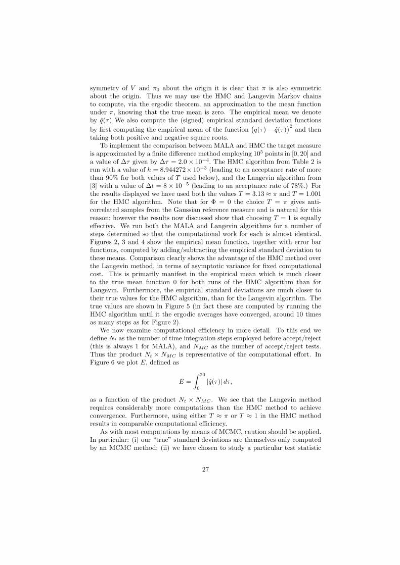
is approximated by a finite difference method employing 105 points in [0, 20] anda value of ∆τ given by ∆τ = 2.0 × 10−4. The HMC algorithm from Table 2 isrun with a value of h = 8.944272× 10−3 (leading to an acceptance rate of morethan 90% for both values of T used below), and the Langevin algorithm from[3] with a value of ∆t = 8 × 10−5 (leading to an acceptance rate of 78%.) Forthe results displayed we have used both the values T = 3.13 ≈ π and T = 1.001for the HMC algorithm. Note that for Φ = 0 the choice T = π gives anti-correlated samples from the Gaussian reference measure and is natural for thisreason; however the results now discussed show that choosing T = 1 is equallyeffective. We run both the MALA and Langevin algorithms for a number ofsteps determined so that the computational work for each is almost identical.Figures 2, 3 and 4 show the empirical mean function, together with error barfunctions, computed by adding/subtracting the empirical standard deviation tothese means. Comparison clearly shows the advantage of the HMC method overthe Langevin method, in terms of asymptotic variance for fixed computationalcost. This is primarily manifest in the empirical mean which is much closerto the true mean function 0 for both runs of the HMC algorithm than forLangevin. Furthermore, the empirical standard deviations are much closer totheir true values for the HMC algorithm, than for the Langevin algorithm. Thetrue values are shown in Figure 5 (in fact these are computed by running theHMC algorithm until it the ergodic averages have converged, around 10 timesas many steps as for Figure 2).

We now examine computational efficiency in more detail. To this end wedefine Nt as the number of time integration steps employed before accept/reject(this is always 1 for MALA), and NMC as the number of accept/reject tests.Thus the product Nt × NMC is representative of the computational effort. InFigure 6 we plot E, defined as

E =

∫ 20

0

|q(τ)| dτ,

as a function of the product Nt × NMC . We see that the Langevin methodrequires considerably more computations than the HMC method to achieveconvergence. Furthermore, using either T ≈ π or T ≈ 1 in the HMC methodresults in comparable computational efficiency.

As with most computations by means of MCMC, caution should be applied.In particular: (i) our “true” standard deviations are themselves only computedby an MCMC method; (ii) we have chosen to study a particular test statistic

27

Figure 2: Empirical mean function, and empirical standard deviation functions, for Hilbertspace-valued HMC algorithm, with T ≈ π.

(the mean function) which possesses a high degree of symmetry so that conclu-sions could differ if a different experiment were chosen. However our experiencewith problems of this sort leads us to believe that the preliminary numericalindications do indeed show the favorable properties of the function space HMCmethod over the function space MALA method.

6. Conclusions

We have suggested (see Table 2) and analyzed a generalized HMC algorithmthat may be applied to sample from Hilbert-space probability distributions πdefined by a density with respect to a Gaussian measure π0 as in (1). In practicethe algorithm has to be applied to a discretized N -dimensional version πN of π,but the fact that the algorithm is well defined in the limit case N = ∞ ensuresthat its performance when applied to sample from πN does not deteriorate asN increases. In this way, and as shown experimentally in Section 5, the newalgorithm eliminates a shortcoming of the standard HMC when used for largevalues of N . On the other hand, we have also illustrated numerically how thealgorithm suggested here benefits from the rationale behind all HMC methods:the capability of taking nonlocal steps when generating proposals alleviates therandom-walk behaviour of other MCMC algorithms; more precisely we haveshown that the Hilbert-space HMC method clearly improves on a Hilbert-spaceMALA counterpart in an example involving conditioned diffusions.

28

Figure 3: Empirical mean function, and empirical standard deviation functions, for Hilbertspace-valued HMC algorithm, with T ≈ 1.

Figure 4: Empirical mean function, and empirical standard deviation functions, for Hilbertspace-valued Langevin algorithm.

29

Figure 5: Mean function and standard deviation functions under the target measure.

Figure 6: Comparison of the computational efficiencies of the two methods.

30

In order to define the algorithm we have successively addressed three issues:

• The definition of a suitable enlarged phase space for the variables q andv = dq/dt and of corresponding measures Π0 and Π having π0 and π,respectively, as marginals on q. The probability measure Π is invariantwith respect to the flow of an appropriate Hamiltonian system. Since theHamiltonian itself is almost surely infinite under Π this result is provedby finite dimensional approximation and passage to the limit.

• A geometric numerical integrator to simulate the flow. This integratoris reversible and symplectic and, when applied in finite-dimensions, alsovolume-preserving. It preserves the measure Π exactly in the particularcase Π = Π0 and approximately in general. The integrator is built on theidea of Strang’s splitting, see e.g. [25], [11]; more sophisticated splittingsare now commonplace and it would be interesting to consider them aspossible alternatives to the method used here.

• We have provided an accept/reject strategy that results in an algorithmthat generates a chain reversible with respect to π. Here we note thatstraightforward generalizations of the formulae employed to accept/rejectin finite dimensions are not appropriate in the Hilbert space context, as theHamiltonian (energy) is almost surely infinite. However for our particularsplitting method the energy difference along the trajectory is finite almostsurely, enabling the algorithm to be defined in the Hilbert space setting.

There are many interesting avenues for future research opened up by thework contained herein. On the theoretical side a major open research programconcerns proving ergodicity for MCMC algorithms applied to measures givenby (1), and the related question of establishing convergence to equilibrium, atN−independent rates, for finite dimensional approximations. Addressing thesequestions is open for the HMC algorithm introduced in this paper, and for theHilbert space MALA algorithms introduced in [3]. The primary theoreticalobstacle to such results is that straightforward minorization conditions can bedifficult to establish in the absence of a smoothing component in the proposal,due to a lack of absolute continuity of Gaussian measures with mean shiftsoutside the Cameron-Martin space. This issue was addressed in continuoustime for the preconditioned Langevin SPDE in the paper [12], by use of theconcept of “asymptotic strong Feller”; it is likely that similar ideas could beused in the discrete time setting of MCMC. We also remark that our theoreticalanalyses have been confined to covariance operators with algebraically decayingspectrum. It is very likely that this assumption may be relaxed to cover super-algebraic decay of the spectrum and this provides an interesting direction forfurther study.

There are also two natural directions for research on the applied side of thiswork. First we intend to use the new HMC method to study a variety of appli-cations with the structure given in (1), such as molecular dynamics and inverseproblems in partial differential equations, with applications to fluid mechanics

31

and subsurface geophysics. Secondly we intend to explore further enhance-ments of the new HMC method, for example by means of more sophisticatedtime-integration methods.

Appendix: Hamiltonian formalism

In this appendix we have collected a number of well-known facts from theHamiltonian formalism (see e.g. [25]) that, while being relevant to the paper,are not essential for the definition of the Hilbert-space algorithm.

To each real-valued function H(z) on the Euclidean space R2N there corre-

spond a canonical Hamiltonian system of differential equations :

dz

dt= J−1∇zH(z) ,

where J is the skew-symmetric matrix

J =

(0N −IN

IN 0N

).

This system conserves the value of H , i.e. H(z(t)) remains constant along solu-tions of the system. Of more importance is the fact that the flow of the canonicalequations preserves the standard or canonical symplectic structure in R

2N , de-fined by the matrix J , or, in the language of differential forms, preserves theassociated canonical differential form Ω. As a consequence the exterior powersΩn, n = 2, . . . , N are also preserved (Poincare integral invariants). The conser-vation of the N -th power corresponds to conservation of the volume element dz.For the Hamiltonian function (3), with z = (q, p), the canonical system is givenby (4).

There are many non-canonical symplectic structures in R2N . For instance,

the matrix J may be replaced by

J =

(0N −LL 0N

),

with L an invertible symmetric N × N real matrix. Then the Hamiltoniansystem corresponding to the Hamiltonian function H is given by

dz

dt= J−1∇zH(z) .

Again H is an invariant of the system and there is a differential form Ω that ispreserved along with its exterior powers Ωn, n = 2, . . . , N . The N -th power is aconstant multiple of the volume element4 dz and therefore the standard volumeis also preserved. With this terminology, the system (10) for the unknown

4In fact, any two non-zero 2N-forms in R2N differ only by a constant factor.

32

z = (q, v), that was introduced through a change of variables in the canonicalHamiltonian system (9), is a (non-canonical) Hamiltonian system on its ownright for the Hamiltonian function (11).

These considerations may be extended to a Hilbert space setting in an ob-vious way. Thus (18) is the Hamiltonian system in H × H arising from theHamiltonian function H in (20) and the structure operator matrix

J =

(0 −C−1

C−1 0

).

However both H and the bilinear symplectic form defined by J , though denselydefined in H ×H, are almost surely infinite in our context, as they only makesense in the Cameron-Martin space.

The splitting of (18) into (21) and (22) used to construct the Hilbert spaceintegrator corresponds to the splitting

H = H1 + H2, H1(q, v) = Φ(q), H2(q, v) =1

2〈v, C−1v〉 +

1

2〈q, C−1q〉

of the Hamiltonian function and therefore the flows Ξt1 and Ξt

2 in (23) and(24) are symplectic. The integrator Ψh is then symplectic as composition ofsymplectic mappings.

Acknowledgements The work of Sanz-Serna is supported by MTM2010-18246-C03-01 (Ministerio de Ciencia e Innovacion). The work of Stuart is suppportedby the EPSRC and the ERC. The authors are grateful to the referees and edi-tor for careful reading of the manuscript, and for many helpful suggestions forimprovement.

References

[1] A. Beskos, N.S. Pillai, G.O. Roberts, J.M. Sanz-Serna, A.M. Stuart, Opti-mal Tuning of Hybrid Monte-Carlo, Technical Report, 2010. Submitted.

[2] A. Beskos, G.O. Roberts, A.M. Stuart, Optimal scalings for localMetropolis-Hastings chains on non-product targets in high dimensions,Ann. Appl. Probab. 19 (2009) 863–898.

[3] A. Beskos, G.O. Roberts, A.M. Stuart, J. Voss, MCMC methods for diffu-sion bridges, Stoch. Dyn. 8 (2008) 319–350.

[4] A. Beskos, A.M. Stuart, MCMC methods for sampling function space,in: R. Jeltsch, G. Wanner (Eds.), Invited Lectures, Sixth InternationalCongress on Industrial and Applied Mathematics, ICIAM07, EuropeanMathematical Society, 2009, pp. 337–364.

33

[5] A. Beskos, A.M. Stuart, Computational complexity of Metropolis-Hastingsmethods in high dimensions, in: P. L’Ecuyer, A.B. Owen (Eds.), MonteCarlo and Quasi-Monte Carlo Methods 2008, Springer-Verlag, 2010.

[6] V. Bogachev, Gaussian Measures, volume 62 of Mathematical Surveys andMonographs, American Mathematical Society, 1998.

[7] J. Bourgain, Periodic nonlinear Schrodinger equation and invariant mea-sures, Commun. Math. Phys. 166 (1994) 1–26.

[8] G. Da Prato, J. Zabczyk, Stochastic equations in infinite dimensions, vol-ume 44 of Encyclopedia of Mathematics and its Applications, CambridgeUniversity Press, Cambridge, 1992.

[9] S. Duane, A.D. Kennedy, B. Pendleton, D. Roweth, Hybrid Monte Carlo,Phys. Lett. B 195 (1987) 216–222.

[10] M. Girolami, B. Calderhead, Riemann manifold Langevin and HamiltonianMonte Carlo methods, Journal of the Royal Statistical Society: Series B(Statistical Methodology) 73 (2011) 123–214.

[11] E. Hairer, C. Lubich, G. Wanner, Geometric numerical integration, vol-ume 31 of Springer Series in Computational Mathematics, Springer-Verlag,Berlin, second edition, 2006. Structure-preserving algorithms for ordinarydifferential equations.

[12] M. Hairer, A.M. Stuart, J. Voss, Analysis of spdes arising in path samplingpart ii: the nonlinear case, Ann. App. Prob. 17 (2010) 1657–1706.

[13] M. Hairer, A.M. Stuart, J. Voss, Signal processing problems on functionspace: Bayesian formulation, stochastic pdes and effective MCMC meth-ods, in: D. Crisan, B. Rozovsky (Eds.), Oxford Handbook of NonlinearFiltering.

[14] A. Irback, Hybrid monte carlo simulation of polymer chains, The Journalof chemical physics 101 (1994) 1661–1667.

[15] J.L. Lebowitz, H.A. Rose, E.R. Speer, Statistical mechanics of the nonlinearschrodinger equation, J. Stat. Phys. 50 (1988) 657–687.

[16] M.A. Lifshits, Gaussian Random Functions, volume 322 of Mathematicsand its Applications, Kluwer, 1995.

[17] J.S. Liu, Monte Carlo strategies in scientific computing, Springer Series inStatistics, Springer, New York, 2008.

[18] B. Mehlig, D.W. Heermann, B.M. Forrest, Exaxct langevin algorithms,Molecular Physics 8 (1992) 1347–1357.

34

[19] R.M. Neal, Probabilistic Inference Using Markov chain Monte Carlo meth-ods, Technical Report, Department of Computer Science, University ofToronto, 1993.

[20] R.M. Neal, MCMC using Hamiltonian dynamics, in: S. Brooks, A. Gelman,G. Jones, X.L. Meng (Eds.), Handbook of Markov Chain Monte Carlo.

[21] K.R. Parthasarathy, Probability measures on metric spaces, Probabilityand Mathematical Statistics, No. 3, Academic Press Inc., New York, 1967.

[22] G.O. Roberts, A. Gelman, W.R. Gilks, Weak convergence and optimalscaling of random walk Metropolis algorithms, Ann. Appl. Probab. 7 (1997)110–120.

[23] G.O. Roberts, J.S. Rosenthal, Optimal scaling of discrete approximationsto Langevin diffusions, J. R. Stat. Soc. Ser. B Stat. Methodol. 60 (1998)255–268.

[24] J.C. Robinson, Infinite Dimensional Dynamical Systems, Cambridge Textsin Applied Mathematics, Cambridge University Press, 2001.

[25] J.M. Sanz-Serna, M.P. Calvo, Numerical Hamiltonian problems, volume 7of Applied Mathematics and Mathematical Computation, Chapman & Hall,London, 1994.

[26] C. Schutte, Conformational dynamics: Modelling, theory, algorithm, andapplication to biomolecules (1998). Habilitation Thesis, Dept. of Math-ematics and Computer Science, Free University Berlin, Available athttp://proteomics-berlin.de/89/.

[27] A.M. Stuart, Inverse problems: a Bayesian approach, Acta Numerica 19(2010).

35