1

Hydraulic Fracturing:

An overview and a Geomechanical approach

Miguel Medinas

Lisbon University, Instituto Superior Técnico (IST), Department of Civil, Architecture and Georesources

The exploitation of unconventional reservoirs, made possible by stimulation using the hydraulic fracturing technique and application of horizontal directional drilling, defines a new era in the global energetic paradigm. Due to the costs of these operations and the specificities of unconventional reservoirs, the industry is required to invest in the development of reliable predictive tools to pre-design these operations. To improve the predictions of the operation outcome oriented perforations are often used. However, the determination of the in-situ stresses and the principal directions is complex; therefore it is important to understand the effect of the perforation orientation on the behavior of induced fractures, in terms of their initiation and propagation, to ensure the success of hydraulic fracturing operations and that the exploration of these fields is economically viable. Using the XFEM method (Extended Finite Element Method) available in Abaqus developed by Dassault Systémes, this thesis presents a numerical study on the mechanical behavior of induced fractures that make use of perforations with different orientations, in particular the conditions of fracture initiation and propagation. To validate the numerical tools, numerical simulations of a series of laboratory tests that reproduce hydraulic fracturing on rectangular blocks of gypsum cement (Abass H. et al, 1994) were carried out. Despite the simplifications of the numerical model, in particular the fact that the fracturing fluid was modelled as a pressure applied in the wellbore, the numerical results provide a good match to the experimental observations. The same numerical model was employed to carry out a parametric study on the effect of a number of relevant parameters on fracture initiation and propagation, namely perforation length, stress anisotropy, wellbore radius and phasing misalignment. The results of this study show that the breakdown pressure is strongly dependent on the tangential stresses at the crack tip, while reorientation is controlled by the principal stress direction anisotropy at the fracture tip, and thus both aspects are determined by the stress state in the near-wellbore zone. In addition, it is found that, when there is perforation misalignment relative to the preferred fracture plane, the density of perforations does not influence the breakdown pressure, but the initiation of the remaining fractures becomes more difficult as the density increases. Keywords: Hydraulic fracturing, oriented Perforations, fracture, Abaqus, XFEM, geomechanics.

1. Introduction Unconventional reservoirs such as coal beds, tight sands and shales have been a growing source of natural gas in the United States (USA) in the last decade (Caldwell, 1997). Shale gas refers to natural gas trapped within shale formations, typically thousands of meters below the earth’s surface. Shales have low permeability, typically between 0,000001mD to 0,0001mD; in comparison to conventional Sandstone reservoirs with a permeability ranges from 0,5 mD to 20 mD (King G. E., 2012). To ensure the economic feasibility of shale gas exploration it is necessary to increase the rock’s permeability. This can be achieved using stimulation by hydraulic fracturing and horizontal drilling) (Bohm, 2008). Hydraulic fracturing operation has been performed since the early days of the petroleum industry. The first experimental test was done in 1947, on a gas well operated by the company Stanolind Oil in the Hugoton field in Grant County, Kansas, USA (Holditch, 2007). In 1949, the company Halliburton Oil Well cementing Company (HOWCO), the exclusive patent holder, performed a total of 332 wells stimulation, with an average production increase of 75%. Over the years, the scientific community has devoted to the development of the technique. Due to the evolution of mathematical models, fluids, materials and equipment, it has become common practice in the industry today and stands out as one of most effective methods providing the opening of exploratory horizon, regarding mainly natural gas reservoirs (Thomas et al, 2001). Hydraulic fracturing (HF) is a formation stimulation practice used to increase the permeability of a producing formation, for hydrocarbons to flow more easily toward the wellbore (Veatch et al, 1989. Hydraulic fracturing consists in applying a pressure higher than the formation strength (breakdown pressure) causing the formation to fracture. Then, a specified fluid volume is pumped and propagated through the opened cracks, creating high flow channels for HC extraction. As result of Drilling technological advances, HF is combined with directional drilling techniques, which increase to 25 times the productive capacity of a well, and wherein the constructive process

is essential to achieve good results in production. In order to predict the result of these operations from the fracture mechanics point of view (initiation and propagation) and its integration into a geomechanical model, numerical simulation tools such as the finite element method (FEM) are frequently used. FEM is found to provide good results in terms of solution convergence and accuracy. In 2009, Abaqus developer Dassault Systemes, have launched a new numerical methodology / functionality, denominated extended finite element method (XFEM), with direct application to fracture analysis that facilitates the modeling process. This functionality introduces a new way to deal with discontinuities / singularities, with a total independence of the fracture to the model, due to the introduction of the concepts partition of unity and introduction of enriched additional degrees of freedom. These eliminate the previously necessary re-meshing process in fracture propagation studies, allowing the reduction of time and memory consumption without loss of accuracy. Since the accurate determination of the in-situ stresses in rock masses is extremely complex, pre-design of the operations aims to improve the results through the control of other parameters or procedures. There emerge the oriented perforation, technology that consists in perforation the rock from the wellbore with pre-defined distances/lengths, widths and directions, to ensure that at least one of the perforations is a few angles of the preferred fracture plane (PFP) in an attempt to reduce the breakdown pressure. Since the excavation of the wellbore introduces a redistribution of stresses near the wellbore, it is essential to study the interaction of perforations with the stress state, in terms of breakdown pressure, fracture geometry and reorientation. The perforation optimal design must ensure the initiation of a single wide fracture with minimum tortuosity, ensuring fracture propagation with minimal injection pressure (Behrmann, 1999). Phasing of 60°, 90°, 120° and 180° are usually the most efficient options for hydraulic fracture treatment because in these directions, the perforation angle and the preferable fracture plane are not very dissimilar, and with such angles the use of several perforation wings reduces the probability of screen out (Aud, 1994).

2

2. Material Behavior

The two basic fluid mechanics variables, injection rates (𝑞𝑖) and fluid viscosity (µ) affect pressure, control the displacement rates of the proppant and have an important role when controlling the fluid loss to the formation. The main objective of HF technique is to increase the permeability of the reservoir, in order to achieve a higher production rate, achieved with the application of the dimensionless fracture conductivity 𝐶𝑓𝐷 concept, which represents the ratio of the

ability of the fracture to carry flow divided by the ability of the formation to feed the fracture.

𝐶𝑓𝐷 =

𝐾𝑓 × 𝑤

𝐾 × 𝑥𝑓

(1)

Where 𝑘𝑓 is the fracture permeability, 𝑤 is the fracture width, 𝐾 is

the reservoir permeability and 𝑥𝑓 is the fracture length. This quantity

is the ratio of the ability of the fracture to carry flow divided by the ability of the formation to feed the fracture, and is a simple measure to quantify the productive capacity of the fracture, depending on its own characteristics as well of the reservoir ones. For high-rate wells, non-Darcy flow can cause an increased pressure drop along the fracture, creating an apparent conductivity and a 𝐶𝑓𝐷

lower than the expected is the regime was laminar, leading to production rates lower than expected (Economides, 2000). Other major complications include non-Darcy or turbulent flow, transient flow regimes, layered reservoirs and horizontal natural permeability anisotropy. Flow is usually defined as the relative sliding of parallel layers, the external forces can be originated from pressure and/or gravity differentials (Poiseuille flow) or from torque (Couette flow). As a reaction, in order to keep the equilibrium of the system, in the opposite direction, the shear stress has the magnitude:

𝜏 = 𝜇 × �̇� (2)

Where 𝜇 is the fluid apparent viscosity and �̇� is the shear rate.The shear rate is defines as:

𝛾 ̇ =

∆𝑢

∆𝑦

(3)

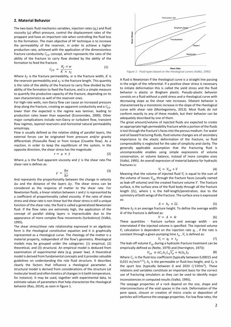
And represents the proportionality between the change in velocity ∆𝑢 and the distance of the layers ∆𝑦. The shear stress can be considered as the response of matter to the shear rate. For Newtonian fluids, a linear relation between 𝜏 and 𝛾 ̇ is represented by a coefficient of proportionality called viscosity. If the ratio of shear stress and shear rate is non-linear but the shear stress is still a unique function of the shear rate, the fluid is called a generalized Newtonian fluid. If the flow rates are extremely high, the application of the concept of parallel sliding layers is impracticable due to the appearance of more complex flow movements (turbulence) (Valkó, 1995). The shear stress/shear rate relationship expressed in an algebraic form is the rheological constitutive equation and it is graphically represented as a rheological curve. The rheology of the matter is a material property, independent of the flow’s geometry. Rheological models may be grouped under the categories: (1) empirical, (2) theoretical, and (3) structural. An empirical model is deduced from examination of experimental data (e.g. power law). A theoretical model is derived from fundamental concepts and it provides valuable guidelines on understanding the role fluid structure. It describes clearly the factors that influence a rheological parameter. A structural model is derived from considerations of the structure (at molecular level) and often kinetics of changes in it (with temperature, for instance). It may be used, together with experimental data, to estimate values of parameters that help characterize the rheological behavior (Rao, 2014), as seen in figure 1.

Figure 1 - Fluid types based on the rheological curves (Valkó, 1995)

A fluid is Newtonian if the rheological curve is a straight line passing in the origin of the referential. If a positive shear stress is necessary to initiate deformation this is called the yield stress and the fluid behavior is plastic or Bingham plastic. Pseudo-plastic behavior consists on a fluid without a yield stress and a rheological curve with decreasing slope as the shear rate increases. Dilatant behavior is characterized by a monotonic increase in the slope of the rheological curve with shear rate (Montegomery, 2013). Most fluids do not conform exactly to any of these models, but their behavior can be adequately described by one of them. The great amount/volume of injected fluids are expected to create an appropriate high permeability fracture while a portion of the fluids is lost through the fracture’s faces into the porous medium. For water and oil based fracturing fluids, fluid volume changes are of secondary importance to the elastic deformation of the fracture, so fluid compressibility is neglected for the sake of simplicity and clarity. The generally applicable assumption that the fracturing fluid is uncompressible enables using simple expressions of volume conservation, or volume balance, instead of more complex ones (Valkó, 1995). An overall expression of material balance for hydraulic fractures is:

𝑉𝑖 = 𝑉𝐿𝑝 + 𝑉 (4)

Meaning that the volume of injected fluid 𝑉𝑖 is equal to the sum of the volume of losses 𝑉𝐿𝑝 through the fracture faces (usually named

as leak-off volume) and the created fracture volume 𝑉. The fracture surface, is the surface area of the fluid body through all the fracture length (2L), where L is the half-length/penetration, due to the symmetry of both wings of the fracture. The surface area is expressed as:

𝐴 = ℎ𝑓 × 2𝐿 (5)

Where ℎ𝑓 is an average fracture height. To define the average width

�̅� of the fracture is defined as: 𝑉 = 𝐴 × �̅� (6)

These quantities - fracture surface and average width - are interrelated if the injected volume is specified. The injected volume 𝑉𝑖 calculation is dependent on the injection rate 𝑞𝑖 , if the rate is constant through a given pumping time 𝑡𝑝 , 𝑉𝑖 is defined as:

𝑉𝑖 = 𝑞𝑖 × 𝑡𝑝 (7)

The leak-off volume 𝑉𝐿𝑝 during a hydraulic fracture treatment can be

empirically defined as (Nolte, 1979) and (Harrington, 1973): 𝑉𝐿𝑝 ≅ 6𝐶𝐿ℎ𝐿𝐿√𝑡𝑝 + 4𝐿ℎ𝐿𝑆𝑃 (8)

Where 𝐶𝐿 is the fluid-loss coefficient (typically between 0,00015 and

0,015 𝑚/𝑚𝑖𝑛1/2), ℎ𝐿 is the permeable or fluid-loss height, and 𝑆𝑃 is the spurt loss (typically between 0 and 2033 𝑙/100𝑚2). These relations and variables constitute an important basis for the correct use of fracturing simulators as they can be used to identify major

inconsistencies in computed results (Valkó, 1995). The seepage properties of a rock depend on the size, shape and interconnections of the void spaces in the rock. Deformation of the pore space, closure or creation of micro cracks or deposition of particles will influence the seepage properties. For low flow rates, the

3

relation between the flow velocity vector 𝑞 and the pore pressure 𝑃𝑝,

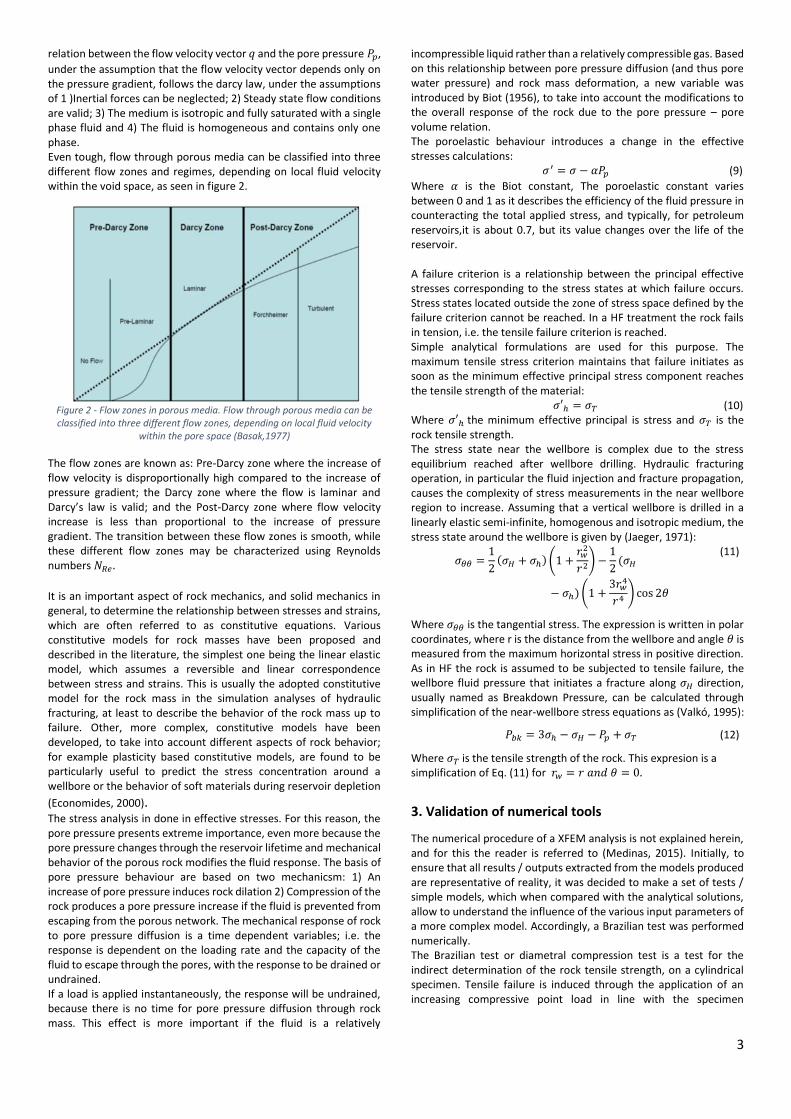
under the assumption that the flow velocity vector depends only on the pressure gradient, follows the darcy law, under the assumptions of 1 )Inertial forces can be neglected; 2) Steady state flow conditions are valid; 3) The medium is isotropic and fully saturated with a single phase fluid and 4) The fluid is homogeneous and contains only one phase. Even tough, flow through porous media can be classified into three different flow zones and regimes, depending on local fluid velocity within the void space, as seen in figure 2.

Figure 2 - Flow zones in porous media. Flow through porous media can be classified into three different flow zones, depending on local fluid velocity

within the pore space (Basak,1977)

The flow zones are known as: Pre-Darcy zone where the increase of flow velocity is disproportionally high compared to the increase of pressure gradient; the Darcy zone where the flow is laminar and Darcy’s law is valid; and the Post-Darcy zone where flow velocity increase is less than proportional to the increase of pressure gradient. The transition between these flow zones is smooth, while these different flow zones may be characterized using Reynolds numbers 𝑁𝑅𝑒 .

It is an important aspect of rock mechanics, and solid mechanics in general, to determine the relationship between stresses and strains, which are often referred to as constitutive equations. Various constitutive models for rock masses have been proposed and described in the literature, the simplest one being the linear elastic model, which assumes a reversible and linear correspondence between stress and strains. This is usually the adopted constitutive model for the rock mass in the simulation analyses of hydraulic fracturing, at least to describe the behavior of the rock mass up to failure. Other, more complex, constitutive models have been developed, to take into account different aspects of rock behavior; for example plasticity based constitutive models, are found to be particularly useful to predict the stress concentration around a wellbore or the behavior of soft materials during reservoir depletion

(Economides, 2000). The stress analysis in done in effective stresses. For this reason, the pore pressure presents extreme importance, even more because the pore pressure changes through the reservoir lifetime and mechanical behavior of the porous rock modifies the fluid response. The basis of pore pressure behaviour are based on two mechanicsm: 1) An increase of pore pressure induces rock dilation 2) Compression of the rock produces a pore pressure increase if the fluid is prevented from escaping from the porous network. The mechanical response of rock to pore pressure diffusion is a time dependent variables; i.e. the response is dependent on the loading rate and the capacity of the fluid to escape through the pores, with the response to be drained or undrained. If a load is applied instantaneously, the response will be undrained, because there is no time for pore pressure diffusion through rock mass. This effect is more important if the fluid is a relatively

incompressible liquid rather than a relatively compressible gas. Based on this relationship between pore pressure diffusion (and thus pore water pressure) and rock mass deformation, a new variable was introduced by Biot (1956), to take into account the modifications to the overall response of the rock due to the pore pressure – pore volume relation. The poroelastic behaviour introduces a change in the effective stresses calculations:

𝜎′ = 𝜎 − 𝛼𝑃𝑝 (9)

Where 𝛼 is the Biot constant, The poroelastic constant varies between 0 and 1 as it describes the efficiency of the fluid pressure in counteracting the total applied stress, and typically, for petroleum reservoirs,it is about 0.7, but its value changes over the life of the reservoir. A failure criterion is a relationship between the principal effective stresses corresponding to the stress states at which failure occurs. Stress states located outside the zone of stress space defined by the failure criterion cannot be reached. In a HF treatment the rock fails in tension, i.e. the tensile failure criterion is reached. Simple analytical formulations are used for this purpose. The maximum tensile stress criterion maintains that failure initiates as soon as the minimum effective principal stress component reaches the tensile strength of the material:

𝜎′ℎ = 𝜎𝑇 (10) Where 𝜎′ℎ the minimum effective principal is stress and 𝜎𝑇 is the rock tensile strength. The stress state near the wellbore is complex due to the stress equilibrium reached after wellbore drilling. Hydraulic fracturing operation, in particular the fluid injection and fracture propagation, causes the complexity of stress measurements in the near wellbore region to increase. Assuming that a vertical wellbore is drilled in a linearly elastic semi-infinite, homogenous and isotropic medium, the stress state around the wellbore is given by (Jaeger, 1971):

𝜎𝜃𝜃 =1

2(𝜎𝐻 + 𝜎ℎ) (1 +

𝑟𝑤2

𝑟2) −

1

2(𝜎𝐻

− 𝜎ℎ) (1 +3𝑟𝑤

4

𝑟4 ) cos 2𝜃

(11)

Where 𝜎𝜃𝜃 is the tangential stress. The expression is written in polar coordinates, where r is the distance from the wellbore and angle 𝜃 is measured from the maximum horizontal stress in positive direction. As in HF the rock is assumed to be subjected to tensile failure, the wellbore fluid pressure that initiates a fracture along 𝜎𝐻 direction, usually named as Breakdown Pressure, can be calculated through simplification of the near-wellbore stress equations as (Valkó, 1995):

𝑃𝑏𝑘 = 3𝜎ℎ − 𝜎𝐻 − 𝑃𝑝 + 𝜎𝑇 (12)

Where 𝜎𝑇 is the tensile strength of the rock. This expresion is a simplification of Eq. (11) for 𝑟𝑤 = 𝑟 𝑎𝑛𝑑 𝜃 = 0.

3. Validation of numerical tools

The numerical procedure of a XFEM analysis is not explained herein, and for this the reader is referred to (Medinas, 2015). Initially, to ensure that all results / outputs extracted from the models produced are representative of reality, it was decided to make a set of tests / simple models, which when compared with the analytical solutions, allow to understand the influence of the various input parameters of a more complex model. Accordingly, a Brazilian test was performed numerically. The Brazilian test or diametral compression test is a test for the indirect determination of the rock tensile strength, on a cylindrical specimen. Tensile failure is induced through the application of an increasing compressive point load in line with the specimen

4

diameter, under controlled temperature (between 5 ° C and 25 ° C) and loading rate (constant strain rate of (50 ± 2) mm / min). The test is carried out in a Marshall test press (typical for Brazilian tests on bituminous mixtures) or similar equipment. The thickness/diameter ratio should be 0.5 to 0.6 for a typical sample diameter of 70 - 160 mm. The sample should be aligned with the lower platen for the load to be applied diametrically. Subsequently the specimen/sample test compression starts. After a period of less than 20% of the loading time period (accordingly to ASTM), a diametrical load at a constant strain rate of (50 ± 2) mm / min is applied continuously and without spiking, until it reaches the maximum load. For each sample, the indirect tensile strength, ITS, is calculated with the following expression, assuming that failure occurs along a clean break (Hudson, 1997):

𝜎𝑡 =

2𝑃

𝜋𝐷𝑡

(13)

Where 𝜎𝑡 is the tensile stress at failure, 𝑃 is the load on the disc at failure, 𝐷 is the disc diameter and 𝑡 is the disc thickness. The behavior of a specimen during a diametral compression test was simulated using the Abaqus software, version 6.14, using the parameters given in table 1.

Table 1 - Input parameters for Brazilian test setup

𝑬(𝑲𝒑𝒂) 𝟏. 𝟒𝟐𝟕 × 𝟏𝟎𝟕 𝑲𝒑𝒂 𝝊 0,2

𝝈𝒕(𝑲𝒑𝒂) 5560 𝐾𝑝𝑎 𝝓 0,265

𝑫(𝒎𝒎) Variable - 80 , 100, 120,160 and 200 mm

𝐭(𝒎) 1

To guarantee the verticality of the sample and ensure that there is no rigid body movement, in the upper point rotation and horizontal displacement was prevented and in the bottom of the specimen all degrees of freedom were restricted to a group of points in order to reduce sample deformability in the bottom of the specimen. With regard to the applied loads, it was decided to apply a load of 5000 kN/min. The adopted finite element mesh was generated using a free meshing procedure available in the software; it is composed by 1327 linear quadrilateral elements with reduced integration and 1385 nodes, independently of the specimen size. The specimen was modelled as a linear elastic material with a damage law for traction separation. Given the loading characteristics, the MAXPS (Maximum principal stress) failure criterion is adopted. This is mathematically described as:

𝑀𝐴𝑋𝑃𝑆 = 𝑀𝑎𝑥𝑖𝑚𝑢𝑚 𝑝𝑟𝑖𝑛𝑐𝑖𝑝𝑎𝑙 𝑠𝑡𝑟𝑒𝑠𝑠 = 𝑓 = {⟨𝜎𝑚𝑎𝑥⟩

𝜎𝑚𝑎𝑥0 }

Where the symbol ⟨ ⟩ is the Macaulay bracket and is used to show that a compressive stress state does not initiate damage, only a tensile stress does it, and a fracture is initiated or the length of an existing fracture is extended after equilibrium increment when the fracture criterion, f, reaches the value 1.0 within a specified tolerance:

1.0 < 𝑓 < 1.0 + 𝑓𝑡𝑜𝑙 (14) Where 𝑓𝑡𝑜𝑙 is the tolerance for the initiation criterion. As the simulation of fracture propagation can be relatively instable, most author propose a value of 0.2 for the tolerance. In figure 3 are compared the analytical results with the results of numerical simulations. The differences between analytical and numerical values are relatively small, varying between 0.2% and 7.1%, with an average error value of 5.64%. The numerical simulation reproduce well the tests in terms of the value of the failure load and development of the failure mechanism (i.e. initiation and propagation of tension fractures). These results confirm the ability of the XFEM to accurately reproduce fracture initiation and propagation.

Figure 3 - Comparison between analytical/theoretical and numerical results

for the Brazilian test

To examine the validity of LEFM for the same time period (60 sec.), the 0,16m sample was loaded with different values applied linearly over the period. The obtained results for the test are presented in table 2.

Table 2 - Different loading/min and failure for the D=0,16m test

Load(KN/min ) Failure t(s) Expected Failure t(s)

Error(%)

2500 33,11 33,6 1,5%

5000 16,8 16,8 ≈ 0%

15000 5,54 5,6 1,1%

30000 2,75 2,8 1,8%

These differences are related with reasons of the local numerical procedure since the meshes are not the most appropriate for the study. The LEFM behavior is followed by the problem in question, given that it assumes that the software behaves correctly for this principle.

4. Numerical analysis of rock propagation in true triaxial samples

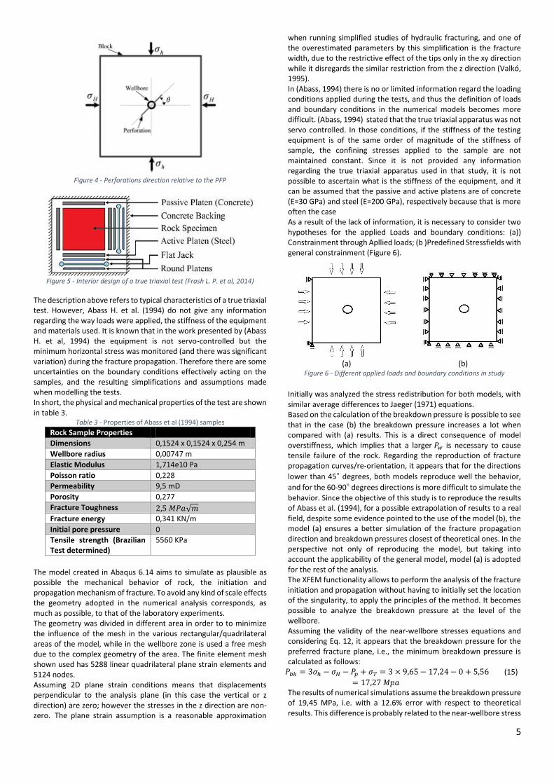
The aim of this section is to simulate numerically, using the Abaqus 6.14 the laboratory experiments described by (Abass et al, 1994) in order to analyze the effect of oriented perforations in drilling wells when using the technique of hydraulic fracturing. This study focuses on phenomena such as the initiation and propagation of hydraulic fractures in vertical wells. The study was conducted using a Shale sample /core with 15,24 cm long and 6,6 cm diameter, openned in the middle along the wellbore direction so that perforations could be executed in directions to study. So that samples could be sealed and used / tested on the device for this purpose, have been merged into Hydrostone (Gypsum cement) in a water weight / Hydrostone ratio 32: 100, in the form of blocks of dimensions 0.154 m x 0.154 m 0,254 m. The study focused on the perforations at a 180-degrees phasing, having been studied the directions (θ) 0, 15, 30, 45, 60, 75 and 90 degrees relative to the PFP (Preferred fracture plane = Maximum horizontal stress =𝜎𝐻), as seen in figure 4. The diameter of the assayed perforations was 3.429 mm.

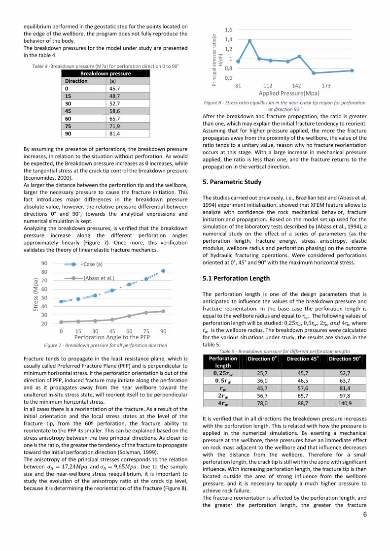
The samples were confined in a true triaxial apparatus with the principal stress applied were: 20670 kPa vertical stress, 17240 KPa maximum horizontal stress and 9650 KPa minimum horizontal stress. True-triaxial loading is typically applied through a series of rigid platens, flexible bladders and passive confinement (e.g. steel casing), as seen in figure 5.

600

800

1000

1200

1400

1600

1800

0,08 0,1 0,12 0,14 0,16 0,18 0,2

Load

(K

N)

Diameter(m)

Analiticalresults

Numericalresults

5

Figure 4 - Perforations direction relative to the PFP

Figure 5 - Interior design of a true triaxial test (Frash L. P. et al, 2014)

The description above refers to typical characteristics of a true triaxial test. However, Abass H. et al. (1994) do not give any information regarding the way loads were applied, the stiffness of the equipment and materials used. It is known that in the work presented by (Abass H. et al, 1994) the equipment is not servo-controlled but the minimum horizontal stress was monitored (and there was significant variation) during the fracture propagation. Therefore there are some uncertainties on the boundary conditions effectively acting on the samples, and the resulting simplifications and assumptions made when modelling the tests. In short, the physical and mechanical properties of the test are shown in table 3.

Table 3 - Properties of Abass et al (1994) samples

Rock Sample Properties

Dimensions 0,1524 x 0,1524 x 0,254 m

Wellbore radius 0,00747 m

Elastic Modulus 1,714e10 Pa

Poisson ratio 0,228

Permeability 9,5 mD

Porosity 0,277

Fracture Toughness 2,5 𝑀𝑃𝑎√𝑚 Fracture energy 0,341 KN/m

Initial pore pressure 0

Tensile strength (Brazilian Test determined)

5560 KPa

The model created in Abaqus 6.14 aims to simulate as plausible as possible the mechanical behavior of rock, the initiation and propagation mechanism of fracture. To avoid any kind of scale effects the geometry adopted in the numerical analysis corresponds, as much as possible, to that of the laboratory experiments. The geometry was divided in different area in order to to minimize the influence of the mesh in the various rectangular/quadrilateral areas of the model, while in the wellbore zone is used a free mesh due to the complex geometry of the area. The finite element mesh shown used has 5288 linear quadrilateral plane strain elements and 5124 nodes. Assuming 2D plane strain conditions means that displacements perpendicular to the analysis plane (in this case the vertical or z direction) are zero; however the stresses in the z direction are non-zero. The plane strain assumption is a reasonable approximation

when running simplified studies of hydraulic fracturing, and one of the overestimated parameters by this simplification is the fracture width, due to the restrictive effect of the tips only in the xy direction while it disregards the similar restriction from the z direction (Valkó, 1995). In (Abass, 1994) there is no or limited information regard the loading conditions applied during the tests, and thus the definition of loads and boundary conditions in the numerical models becomes more difficult. (Abass, 1994) stated that the true triaxial apparatus was not servo controlled. In those conditions, if the stiffness of the testing equipment is of the same order of magnitude of the stiffness of sample, the confining stresses applied to the sample are not maintained constant. Since it is not provided any information regarding the true triaxial apparatus used in that study, it is not possible to ascertain what is the stiffness of the equipment, and it can be assumed that the passive and active platens are of concrete (E=30 GPa) and steel (E=200 GPa), respectively because that is more often the case As a result of the lack of information, it is necessary to consider two hypotheses for the applied Loads and boundary conditions: (a)) Constrainment through Apllied loads; (b )Predefined Stressfields with general constrainment (Figure 6).

(a) (b)

Figure 6 - Different applied loads and boundary conditions in study

Initially was analyzed the stress redistribution for both models, with similar average differences to Jaeger (1971) equations. Based on the calculation of the breakdown pressure is possible to see that in the case (b) the breakdown pressure increases a lot when compared with (a) results. This is a direct consequence of model overstiffness, which implies that a larger 𝑃𝑤 is necessary to cause tensile failure of the rock. Regarding the reproduction of fracture propagation curves/re-orientation, it appears that for the directions

lower than 45° degrees, both models reproduce well the behavior,

and for the 60-90° degrees directions is more difficult to simulate the

behavior. Since the objective of this study is to reproduce the results of Abass et al. (1994), for a possible extrapolation of results to a real field, despite some evidence pointed to the use of the model (b), the model (a) ensures a better simulation of the fracture propagation direction and breakdown pressures closest of theoretical ones. In the perspective not only of reproducing the model, but taking into account the applicability of the general model, model (a) is adopted for the rest of the analysis. The XFEM functionality allows to perform the analysis of the fracture initiation and propagation without having to initially set the location of the singularity, to apply the principles of the method. It becomes possible to analyze the breakdown pressure at the level of the wellbore. Assuming the validity of the near-wellbore stresses equations and considering Eq. 12, it appears that the breakdown pressure for the preferred fracture plane, i.e., the minimum breakdown pressure is calculated as follows:

𝑃𝑏𝑘 = 3𝜎ℎ − 𝜎𝐻 − 𝑃𝑝 + 𝜎𝑇 = 3 × 9,65 − 17,24 − 0 + 5,56

= 17,27 𝑀𝑝𝑎

(15)

The results of numerical simulations assume the breakdown pressure of 19,45 MPa, i.e. with a 12.6% error with respect to theoretical results. This difference is probably related to the near-wellbore stress

6

equilibrium performed in the geostatic step for the points located on the edge of the wellbore, the program does not fully reproduce the behavior of the body. The breakdown pressures for the model under study are presented in the table 4.

Table 4 -Breakdown pressure (M?a) for perforation direction 0 to 90°

Breakdown pressure

Direction (a)

0 45,7

15 48,7

30 52,7

45 58,6

60 65,7

75 71,9

90 81,4

By assuming the presence of perforations, the breakdown pressure increases, in relation to the situation without perforation. As would be expected, the Breakdown pressure increases as θ increases, while the tangential stress at the crack tip control the breakdown pressure (Economides, 2000). As larger the distance between the perforation tip and the wellbore, larger the necessary pressure to cause the fracture initiation. This fact introduces major differences in the breakdown pressure absolute value, however, the relative pressure differential between directions 0° and 90°, towards the analytical expressions and numerical simulation is kept. Analyzing the breakdown pressures, is verified that the breakdown pressure increase along the different perforation angles approximately linearly (Figure 7). Once more, this verification validates the theory of linear elastic fracture mechanics.

Figure 7 - Breakdown pressure for all perforation direction

Fracture tends to propagate in the least resistance plane, which is usually called Preferred Fracture Plane (PFP) and is perpendicular to minimum horizontal stress. If the perforation orientation is out of the direction of PFP, induced fracture may initiate along the perforation and as it propagates away from the near wellbore toward the unaltered in-situ stress state, will reorient itself to be perpendicular to the minimum horizontal stress. In all cases there is a reorientation of the fracture. As a result of the initial orientation and the local stress states at the level of the fracture tip, from the 60º perforation, the fracture ability to reorientate to the PFP its smaller. This can be explained based on the stress anisotropy between the two principal directions. As closer to one is the ratio, the greater the tendency of the fracture to propagate toward the initial perforation direction (Solyman, 1999). The anisotropy of the principal stresses corresponds to the relation between 𝜎𝐻 = 17,24𝑀𝑝𝑎 and 𝜎ℎ = 9,65𝑀𝑝𝑎. Due to the sample size and the near-wellbore stress reequilibrium, it is important to study the evolution of the anisotropy ratio at the crack tip level, because it is determining the reorientation of the fracture (Figure 8).

Figure 8 - Stress ratio equilibrium in the near-crack tip region for perforation

at direction 90°

After the breakdown and fracture propagation, the ratio is greater than one, which may explain the initial fracture tendency to reorient. Assuming that for higher pressure applied, the more the fracture propagates away from the proximity of the wellbore, the value of the ratio tends to a unitary value, reason why no fracture reorientation occurs at this stage. With a large increase in mechanical pressure applied, the ratio is less than one, and the fracture returns to the propagation in the vertical direction.

5. Parametric Study

The studies carried out previously, i.e., Brazilian test and (Abass et al, 1994) experiment initialization, showed that XFEM feature allows to analyze with confidence the rock mechanical behavior, fracture initiation and propagation. Based on the model set up used for the simulation of the laboratory tests described by (Abass et al., 1994), a numerical study on the effect of a series of parameters (as the perforation length, fracture energy, stress anisotropy, elastic modulus, wellbore radius and perforation phasing) on the outcome of hydraulic fracturing operations. Were considered perforations oriented at 0°, 45° and 90° with the maximum horizontal stress.

5.1 Perforation Length

The perforation length is one of the design parameters that is anticipated to influence the values of the breakdown pressure and fracture reorientation. In the base case the perforation length is equal to the wellbore radius and equal to 𝑟𝑤. The following values of perforation length will be studied: 0,25𝑟𝑤, 0,5𝑟𝑤, 2𝑟𝑤 𝑎𝑛𝑑 4𝑟𝑤 where 𝑟𝑤 is the wellbore radius. The breakdown pressures were calculated for the various situations under study, the results are shown in the table 5.

Table 5 - Breakdown pressure for different perforation lengths

Perforation length

Direction 0° Direction 45° Direction 90°

𝟎, 𝟐𝟓𝒓𝒘 25,7 45,7 52,7

𝟎, 𝟓𝒓𝒘 36,0 46,5 63,7

𝒓𝒘 45,7 57,6 81,4

𝟐𝒓𝒘 56,7 65,7 97,8

𝟒𝒓𝒘 78,0 88,7 140,9

It is verified that in all directions the breakdown pressure increases with the perforation length. This is related with how the pressure is applied in the numerical simulations. By exerting a mechanical pressure at the wellbore, these pressures have an immediate effect on rock mass adjacent to the wellbore and that influence decreases with the distance from the wellbore. Therefore for a small perforation length, the crack tip is still within the zone with significant influence. With increasing perforation length, the fracture tip is then located outside the area of strong influence from the wellbore pressure, and it is necessary to apply a much higher pressure to achieve rock failure. The fracture reorientation is affected by the perforation length, and the greater the perforation length, the greater the fracture

20

30

40

50

60

70

80

90

0 15 30 45 60 75 90

Stre

ss (

Mp

a)

Perforation Angle to the PFP

Case (a)

(Abass et al.)

0,6

0,8

1

1,2

1,4

1,6

81 112 142 173Pri

nci

pal

str

esse

s ra

tio

(𝜎H

/𝜎h

)

Applied Pressure(Mpa)

7

reorientation difficulties (Zhang, 2009). The results of the numerical simulation do not show clearly this effect (Figure 9).

Figure 9 - Fracture reorientation from the crack tip for different perforation

lengths to direction 90°

5.2 Fracture Energy

The fracture energy is a parameter that affects the propagation of the fracture. To study its effect are used 0,0341𝐾𝑁/𝑚 , 34,1𝐾𝑁/𝑚, 3410𝐾𝑁/𝑚 beyond the base case already analyzed 𝐺𝑐 = 0,341𝐾𝑁/𝑚. Fracture initiation is reached when tensile failure of the rock occurs, according to equation 6.8. The fracture propagates since then, however, the rock remain with cohesive behavior until is totally damaged, offering resistance to propagation (i.e. for higher fracture energy, the fracture damage is slower and this affects slightly the stress state in the near tip region). This resistance is lost with the continuation of loading, with the rock having an energy-based damage evolution behavior. It appears that the displacements for which there is no further cohesive fracture behavior, are much smaller for low fracture energies and are therefore achieved for lower induced pressures, which increases the fracture propagation velocity (Figure 10).

Figure 10 - Distance-Time for different fracture energies

For small distances from the tip of the perforation, the distance-time relationships are similar. This is the result of applying the pressure in the wellbore, since it is near the wellbore that stresses are high, and so are the deformations. Accordingly, the dependence of fracture energy is smaller (because the fracture still propagates at same magnitude rates for completely different fracture energies). At a larger distance, the effect of the pressure applied at the wellbore is small, and thus a larger pressure is required to cause the strain necessary to reach full damage to cohesive rock behavior.

5.3 Perforation Phasing

In practice, perforation phasing is selected to ensure that with a few degrees difference, there is a perforation in the direction of

maximum horizontal principal stress 𝜎𝐻, with 60°, 90°, 120°, 180° phasing being studied. With the perforation oriented in the direction of the PFP, there are no significant changes in the breakdown

pressure. Even tough, an increment in the breakdown pressure for the second fracture to initiate happens in all situations (table 7).

Table 6 - Second Breakdown pressure (MPa) for different perforation Phasing

Phasing 180° 120° 90° 60°

Breakdown pressure for first fracture

45,7 45,7 45,7 45,7

Breakdown Pressure for second fracture

- 73,8 96,7 82,3

Breakdown Pressure for second fracture if alone

45,7 65,7 81,4 65,7

Relative difference (%) - 12,4 18,8 25,3

It was confirmed that with an increase in perforation density, and an associated reduction in the angle between perforations, the increment in pressure required to produce the propagation of the second fracture increases. Obviously, the second breakdown pressure is also dependent on the perforation direction, however the density in the factor which introduces major differences, as can be

seen comparing the results of the relative difference for phasing 60°

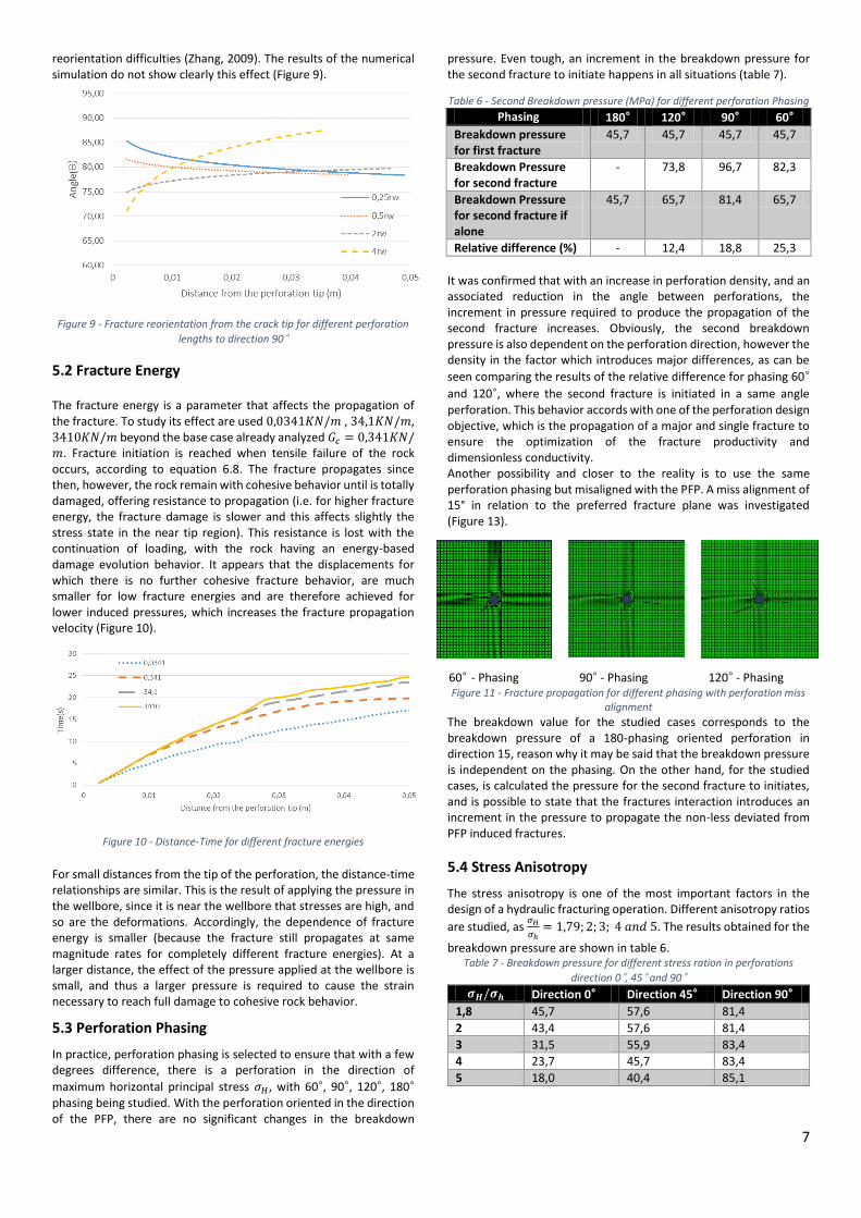
and 120°, where the second fracture is initiated in a same angle perforation. This behavior accords with one of the perforation design objective, which is the propagation of a major and single fracture to ensure the optimization of the fracture productivity and dimensionless conductivity. Another possibility and closer to the reality is to use the same perforation phasing but misaligned with the PFP. A miss alignment of 15° in relation to the preferred fracture plane was investigated (Figure 13).

60° - Phasing 90° - Phasing 120° - Phasing Figure 11 - Fracture propagation for different phasing with perforation miss

alignment

The breakdown value for the studied cases corresponds to the breakdown pressure of a 180-phasing oriented perforation in direction 15, reason why it may be said that the breakdown pressure is independent on the phasing. On the other hand, for the studied cases, is calculated the pressure for the second fracture to initiates, and is possible to state that the fractures interaction introduces an increment in the pressure to propagate the non-less deviated from PFP induced fractures.

5.4 Stress Anisotropy

The stress anisotropy is one of the most important factors in the design of a hydraulic fracturing operation. Different anisotropy ratios

are studied, as 𝜎𝐻

𝜎ℎ= 1,79; 2; 3; 4 𝑎𝑛𝑑 5. The results obtained for the

breakdown pressure are shown in table 6. Table 7 - Breakdown pressure for different stress ration in perforations

direction 0°, 45° and 90°

𝝈𝑯/𝝈𝒉 Direction 0° Direction 45° Direction 90°

1,8 45,7 57,6 81,4

2 43,4 57,6 81,4

3 31,5 55,9 83,4

4 23,7 45,7 83,4

5 18,0 40,4 85,1

8

It is verified that in the 0 direction there is a clear reduction in the breakdown pressure with increasing anisotropy. In direction 45 the reduction is less significant, but still happens. In the direction 90 there is very little change and breakdown pressure suffers even a very small increase with increasing anisotropy. According to the Eq. (12), the breakdown pressure is only dependent of the principal stresses. For perforation direction 0, a reduction in the breakdown pressure would be expected. For the direction 90, and taking into account that there is any reduction of 𝜎𝐻, the theoretical value without perforation of the breakdown pressure in the direction 90 is approximately constant. The model is correctly simulating the behavior for direction 90, without clear changes in the breakdown pressure for this direction. The stress anisotropy has an effect in fracture reorientation (Figure 11 and 12).

𝜎𝐻/𝜎ℎ = 2 𝜎𝐻/𝜎ℎ = 3

𝜎𝐻/𝜎ℎ = 4 𝜎𝐻/𝜎ℎ = 5

Figure 12 - Fracture propagation for different stress ratio in direction 90°

The effect of the reorientation with the stress anisotropy is most

apparent in the 90° direction. This occurs because the stress

equilibrium in the proximity of the fracture in 90° direction ensures the existence of the same order of magnitude of tangential stresses but significant reductions in normal stresses, allowing the fracture to reorientate toward the PFP.

Figure 13 - Fracture reorientation for different stress anisotropies to direction

90°

5.5 Other parameters

Rock elastic modulus was other of the studied parameters, and assuming the LEFM and a linear stress-strain relationship, if the stresses are constant, increasing the elastic modulus, the body strains are reduced. There were no significant changes in the reorientation

of the fracture depending on the elasticity modulus. It was concluded that as higher the elastic modulus, slower is the damage evolution, because it is dependent on the local strains (which by its turn are dependent of the material elasticity). Wellbore radius was another studied parameter, confined to the analysis of a wellbore radius twice (situation b) of the (Abass et al, 1994) experiments. Analyzing the Eq. (15), can be seen that the near-wellbore stresses depend only on the wellbore radius and the principal stresses. However, at the wellbore border, it is comproved that there is no change regarding the previously studied case, and the stresses in the surrounding are re-equilibrated proportionally to the normalized distance to the wellbore center. Table 8 shows the breakdown pressure obtained with no perforation and perforation angles of 0°, 45° and 90° Table 8 - Breakdown pressure (MPa) for different perforation direction with a

wellbore radius (𝑟)

Breakdown pressure

Direction 0° Direction 45° Direction 90° Without Perf.

𝑟 = 0,00747 𝑚 45,7 57,6 81,4 19,45 𝑟 = 0,0149 𝑚 28,70 48,16 53,67 16,71

It is found that increasing the wellbore radius causes the breakdown pressures to reduce. The near-wellbore stress changes are proportional to the normalized distance, and for this situation, while considering the same perforation length for both situations the tangential stresses at the tip of the perforation for situation (b) are higher than in (a). Based on this it would be expected an increase in breakdown pressure with the wellbore radius, but the opposite is observed. During HF simulation, when r = 0,0149 m the applied pressure is being exerted in a doubled wellbore surface, and thus the stress state in the near-wellbore region (and in particular at the perforation tip, because the perforation length has been maintained constant) suffers greater modification and the rock tensile failure is achieved earlier.

6.Conclusions

It is verified that the geomechanical model developed with the use the ABAQUS software, and in particular the XFEM functionality, reproduces with quality the experiences described by Abass et al. (1994), whereby the parametric study conducted is representative of the reality. From this study some conclusions can be drawn: - Perforations along non-preferred directions affect significantly the fracture breakdown pressure and the reorientation procedure. Perforations more deviated from the PFP perforations tend to have higher reorientation difficulties and the breakdown pressure increase is a consequence of the higher tangential stresses in these directions. Fracture initiation for the situation without initial perforation is well reproduced, which corroborates the model representativeness and the capabilities of the numerical tools. - The near-wellbore equations are defined for a situation without any additional loading at the wellbore (i.e. applied pressures); however, the sample is subjected to stress state changes because of the application of the pressure at the wellbore, which affects the results, both in terms of fracture initiation and propagation. - Increasing the perforation length leads to a significant increase in breakdown pressure, but only to a minor reduction in fracture reorientation. This effect is thought to derive from the manner in which loading is applied. - The fracture energy is not an intrinsic rock parameter; therefore, it influences mainly the rate at which damage to fracture cohesive behavior occurs, without any influence in fracture reorientation or in the breakdown pressure.

9

- Higher stress anisotropy ratios increase the capacity of fracture reorientation, with the reorientation to the PFP occurring over a smaller distance. Though in a real situation fracture initiation in directions 60° to 90° is not expected, for those perforations angles the reorientation happens slower due to the high tangential stresses at the fracture tip, which influences (increases) equally the breakdown pressure. - Rock elastic modulus is found to influence the rate at which damage to the fracture cohesive behavior occurs, and cause insignificant changes in fracture reorientation and breakdown pressure. - Changes in the wellbore radius introduces changes in the near-wellbore stress state equilibrium with distance, however the induced stresses are proportional to the normalized distance (normalized by the wellbore radius). The breakdown pressure reduction for a larger wellbore is explained by the fact that the total applied stress is proportional to the wellbore surface. Assuming it is applied at the same rate, a faster stress change (traction generation) is induced and fracture initiates. - Using a perforation higher density increases the probability of a perforation being oriented close to the PFP, optimizing the success of a HF operation. The breakdown pressure of the first fracture (subjected to slower tangential stresses) is not significantly affected by phasing misalignment; however, the initiation of a second fracture tends to suffer an increase in the breakdown pressure. As the objective is to maximize the production, the important fracture is that close to the PFP, because it increases the fracture opening with smaller applied loads, increasing the productivity index and the fracture dimensionless conductivity coefficient. According to the information presented it can be concluded that fracture initiation is largely controlled by the shear stress at the fracture tip, while fracture reorientation depends strongly on the perforation angle and stress anisotropy. Since the model employed relies on the application of a mechanical pressure rather than fluid injection pressures, pressure is not being applied at the fracture tip, which affects the breakdown pressures. It is assumed that the numerical analyses quantify the relative changes in breakdown pressure with increasing perforation angle, but not its absolute value. Since the hydraulic fracturing technique relies on the injection of fluids, and many other fluid parameters (viscosity, specific weight, type of fluid, etc.) can influence the initiation and propagation behavior of induced fractures, a hydro-geomechanical model should be set to study all these parameters. Despite the simplification made in the analyses presented in this thesis, it is considered that this study has contributed to improve our global understanding of the application of hydraulic fracturing technique and the parameters that affects its operation, and thus its primary objectives have been fulfilled.

References Abass H. et al. (1994). Oriented Perforations - A Rock Mechanics View. New

Orleans, Louisiana: Society of Petroleum Engineers. Altmann J., A. (2010). Poroelastic effects in reservoir modelling. Karlsruher

Instituts für Technologie. Basak P., B. (1977). Non-Darcy flow and its implications to seepage problems.

Journal of the Irrigation and Drainage Division (ASCE). Bohm P. et al. (2008). Hydraulic Fracturing Considerations for Natural Gas

Wells of the Fayetteville Shale . ALL Consulting. Caldwell J. et al. (1997). Oilfield Review - Exploring for stratigraphic traps.

Houston, Texas: Schumlberger. Economides M. J. et al. (2000). Reservoir Stimulation. Chicester: John Wiley

and Sons. Frash L. P. et al. (2014). True-triaxial apparatus for simulation of hydraulically

fractured multi-borehole hot dry rock reservoirs. International Journal of Rock Mechanics & Mining Sciences, 496-506.

Harrington L.J. et al. (1973). “Prediction of the Location and Movement of Fluid Interfaces in the Fracture. Southwestern Petroleum short courses. Texas, USA: Texas University.

Hudson J. A. et Harrisson J. P. (1997). Engineering Rock Mechanics: An introduction to the principles. Oxford: Pergamon.

Jaeger J. C. et Cook N. G. W. (1971). FUndamentals of rock mechanics. London: Chapman and Hall Ltd.

King G. E., K. (2012). Thirty years of Shale Gas fracturing: What have we learned? Florence , Italy: SPE annual technical conference and Exhibition.

Medinas M. (2015). An Extended Finite Element Method (XFEM) approach to

hydraulic fractures: Modelling of oriented perforations, IST (Lisbon)

Montegomery C. (2013). Fracturing Fluids. Em Bunger P. A. et al., Effective and Sustainable Hydraulic Fracturing (pp. 3-23). InTech.

Nolte K.G. (1979). Determination of Fracture Parameters from fracture pressure decline. SPE Annual Technical Conference and exhbition. Las Vegas, Nevada: Society of Petroleum Engineers.

Rahman M. K. et Joarder A. H. (2005). Investigating production-induced stress change at fracture tips: Implications for a novel hydraulic fracturing technique. Journal of Petroleum Science and Engineering, 185-196.

Rao M. A. (2014). Rheology of fluid, semisolid, and Solid foods - Principles and applications. Springer.

Solyman M. Y. et Boonen P. (1999). Rock Mechanics and stimulation aspects of horizontal wells. Journal of Petroleum Science and Engineering, 187-204.

Thomas J. et al (2001). Fundamentos de Engenharia de Petróleo. Rio de Janeiro: Editora Interciência

Valkó P. et Economides M. J. (1995). Hydraulic Fracture Mechanics. Chicester: John Wiley and Sons.

Zhang G. et Chen M. (2009). Dynamic fracture propagation in hydraulic re-fracturing. Journal of Petroleum Science and ENgineering, 266-272.

Zoback M. (2007). Reservoir Geomechanics. Cambridge: Cambridge University Press.

Nomenclature

ℎ𝑓 − 𝐹𝑟𝑎𝑐𝑡𝑢𝑟𝑒 ℎ𝑒𝑖𝑔ℎ𝑡

𝐶𝐿 − 𝐹𝑙𝑢𝑖𝑑 𝑙𝑜𝑠𝑠 𝑐𝑜𝑒𝑓𝑓𝑖𝑐𝑖𝑒𝑛𝑡 𝐶𝑓𝑑 − 𝐹𝑟𝑎𝑐𝑡𝑢𝑟𝑒 𝑐𝑜𝑛𝑑𝑢𝑐𝑡𝑖𝑣𝑖𝑡𝑦

𝐾𝑓 − 𝐹𝑟𝑎𝑐𝑡𝑢𝑟𝑒 𝑝𝑒𝑟𝑚𝑒𝑎𝑏𝑖𝑙𝑖𝑡𝑦

𝑁𝑅𝑒 − 𝑅𝑒𝑦𝑛𝑜𝑙𝑑𝑠 𝑁𝑢𝑚𝑏𝑒𝑟 𝑃𝐵𝑘 − 𝐵𝑟𝑒𝑎𝑘𝑑𝑜𝑤𝑛 𝑝𝑟𝑒𝑠𝑠𝑢𝑟𝑒 𝑃𝑃 − 𝑃𝑜𝑟𝑒 𝑝𝑟𝑒𝑠𝑠𝑢𝑟𝑒 𝑃𝑖 − 𝐼𝑛𝑖𝑡𝑖𝑎𝑙 𝑝𝑜𝑟𝑒 𝑝𝑟𝑒𝑠𝑠𝑢𝑟𝑒 𝑆𝑝 − 𝑆𝑝𝑢𝑟𝑡 𝑙𝑜𝑠𝑠

𝑉𝐿𝑝 − 𝑉𝑜𝑙𝑢𝑚𝑒 𝑙𝑜𝑠𝑠𝑒𝑠

𝑉𝑖 − 𝐼𝑛𝑗𝑒𝑐𝑡𝑒𝑑 𝐹𝑙𝑢𝑖𝑑 𝑟𝑤 − 𝑊𝑒𝑙𝑙𝑏𝑜𝑟𝑒 𝑟𝑎𝑑𝑖𝑢𝑠 �̅� − 𝐴𝑣𝑒𝑟𝑎𝑔𝑒 𝑤𝑖𝑡𝑑ℎ 𝑥𝑓 − 𝐹𝑟𝑎𝑐𝑡𝑢𝑟𝑒 𝑙𝑒𝑛𝑔𝑡ℎ

�̇� − 𝑆ℎ𝑒𝑎𝑟 𝑅𝑎𝑡𝑒 𝜎′ − 𝐸𝑓𝑓𝑒𝑐𝑡𝑖𝑣𝑒 𝑠𝑡𝑟𝑒𝑠𝑠

𝜎𝑇 − 𝑅𝑜𝑐𝑘 𝑡𝑒𝑛𝑠𝑖𝑙𝑒 𝑠𝑡𝑟𝑒𝑛𝑔𝑡ℎ 𝜎𝑖𝑗 − 𝑆𝑡𝑟𝑒𝑠𝑠 𝑇𝑒𝑛𝑠𝑜𝑟

𝜎𝑣 − 𝑉𝑒𝑟𝑡𝑖𝑐𝑎𝑙 𝑠𝑡𝑟𝑒𝑠𝑠 < > −𝑀𝑎𝑐𝑎𝑢𝑙𝑎𝑦 𝑏𝑟𝑎𝑐𝑘𝑒𝑡 𝐷 − 𝐷𝑖𝑎𝑚𝑒𝑡𝑒𝑟 𝐸 − 𝐸𝑙𝑎𝑠𝑡𝑖𝑐 𝑀𝑜𝑑𝑢𝑙𝑢𝑠 𝐺 − 𝑆ℎ𝑒𝑎𝑟 𝑀𝑜𝑑𝑢𝑙𝑢𝑠 𝑃 − 𝐿𝑜𝑎𝑑 𝑜𝑛 𝑡ℎ𝑒 𝐷𝑖𝑠𝑐 𝑉 − 𝑉𝑜𝑙𝑢𝑚𝑒 𝑞 − 𝐿𝑖𝑛𝑒𝑎𝑟 𝑓𝑙𝑜𝑤 𝑟𝑎𝑡𝑒 𝑡 − 𝐷𝑖𝑠𝑐 𝑡ℎ𝑖𝑐𝑘𝑛𝑒𝑠𝑠 𝛼 − 𝐵𝑖𝑜𝑡′𝑠 𝑐𝑜𝑒𝑓𝑓𝑖𝑐𝑖𝑒𝑛𝑡 𝜃 − 𝑃𝑒𝑟𝑓𝑜𝑟𝑎𝑡𝑖𝑜𝑛 𝑎𝑛𝑔𝑙𝑒 𝑤𝑖𝑡ℎ 𝑃𝐹𝑃 𝜇 − 𝑣𝑖𝑠𝑐𝑜𝑠𝑖𝑡𝑦 𝜈 − 𝑃𝑜𝑖𝑠𝑠𝑜𝑛 𝑅𝑎𝑡𝑖𝑜 𝜌 − 𝐷𝑒𝑛𝑠𝑖𝑡𝑦 𝜏 − 𝑇𝑎𝑛𝑔𝑒𝑛𝑡𝑖𝑎𝑙 𝑆𝑡𝑟𝑒𝑠𝑠

𝜎ℎ − 𝑀𝑖𝑛𝑖𝑚𝑢𝑚 ℎ𝑜𝑟𝑖𝑧𝑜𝑛𝑡𝑎𝑙 𝑠𝑡𝑟𝑒𝑠𝑠 𝜎𝐻 − 𝑀𝑎𝑥𝑖𝑚𝑢𝑚 ℎ𝑜𝑟𝑖𝑧𝑜𝑛𝑡𝑎𝑙 𝑠𝑡𝑟𝑒𝑠𝑠