hydroclimate variability and long-lead forecasting of...
TRANSCRIPT

This article was downloaded by: [Nkrintra Singhrattna]On: 23 January 2012, At: 16:41Publisher: Taylor & FrancisInforma Ltd Registered in England and Wales Registered Number: 1072954 Registered office: Mortimer House,37-41 Mortimer Street, London W1T 3JH, UK
Hydrological Sciences JournalPublication details, including instructions for authors and subscription information:http://www.tandfonline.com/loi/thsj20
Hydroclimate variability and long-lead forecastingof rainfall over Thailand by large-scale atmosphericvariablesNkrintra Singhrattna a , Mukand S. Babel a & Sylvain R. Perret a ba Water Engineering and Management, Asian Institute of Technology, Pathumthani, Thailandb Centre de Coopération Internationale en Recherche Agronomique pour le Développement,UMR G-Eau, Montpellier, France
Available online: 20 Jan 2012
To cite this article: Nkrintra Singhrattna, Mukand S. Babel & Sylvain R. Perret (2012): Hydroclimate variability and long-leadforecasting of rainfall over Thailand by large-scale atmospheric variables, Hydrological Sciences Journal, 57:1, 26-41
To link to this article: http://dx.doi.org/10.1080/02626667.2011.633916
PLEASE SCROLL DOWN FOR ARTICLE
Full terms and conditions of use: http://www.tandfonline.com/page/terms-and-conditions
This article may be used for research, teaching, and private study purposes. Any substantial or systematicreproduction, redistribution, reselling, loan, sub-licensing, systematic supply, or distribution in any form toanyone is expressly forbidden.
The publisher does not give any warranty express or implied or make any representation that the contentswill be complete or accurate or up to date. The accuracy of any instructions, formulae, and drug doses shouldbe independently verified with primary sources. The publisher shall not be liable for any loss, actions, claims,proceedings, demand, or costs or damages whatsoever or howsoever caused arising directly or indirectly inconnection with or arising out of the use of this material.

26 Hydrological Sciences Journal – Journal des Sciences Hydrologiques, 57(1) 2012
Hydroclimate variability and long-lead forecasting of rainfall overThailand by large-scale atmospheric variables
Nkrintra Singhrattna1, Mukand S. Babel1 and Sylvain R. Perret1,2
1Water Engineering and Management, Asian Institute of Technology, Pathumthani, [email protected], [email protected]
2Centre de Coopération Internationale en Recherche Agronomique pour le Développement, UMR G-Eau, Montpellier, France
Received 27 May 2010; accepted 25 March 2011; open for discussion until 1 July 2012
Editor Z.W. Kundzewicz
Citation Singhrattna, N., Babel, M.S. and Perret, S.R., 2012. Hydroclimate variability and long-lead forecasting of rainfall overThailand by large-scale atmospheric variables. Hydrological Sciences Journal, 57 (1), 26–41.
Abstract The development of statistical relationships between local hydroclimates and large-scale atmosphericvariables enhances the understanding of hydroclimate variability. The rainfall in the study basin (the Upper ChaoPhraya River Basin, Thailand) is influenced by the Indian Ocean and tropical Pacific Ocean atmospheric circu-lation. Using correlation analysis and cross-validated multiple regression, the large-scale atmospheric variables,such as temperature, pressure and wind, over given regions are identified. The forecasting models using atmo-spheric predictors show the capability of long-lead forecasting. The modified k-nearest neighbour (k-nn) model,which is developed using the identified predictors to forecast rainfall, and evaluated by likelihood function, showsa long-lead forecast of monsoon rainfall at 7–9 months. The decreasing performance in forecasting dry-seasonrainfall is found for both short and long lead times. The developed model also presents better performance inforecasting pre-monsoon season rainfall in dry years compared to wet years, and vice versa for monsoon seasonrainfall.
Key words rainfall; hydroclimate variability; ENSO; large-scale atmospheric variables; long-lead forecasting; statisticalapproach; modified k-nn model; cross-validated multiple regression; Chao Phraya River Basin; Ping River Basin; Thailand
Variabilité hydroclimatique et prévision à long terme des précipitations en Thaïlande à l’aide devariables atmosphériques de grande échelleRésumé L’établissement de relations statistiques entre variables pluviométriques locales et variables atmo-sphériques de grande échelle permet une meilleure compréhension de la variabilité hydroclimatique. Lesprécipitations dans le bassin d’étude (le bassin supérieur de la Rivière Chao Phraya, Thaïlande) sont influencéespar la circulation atmosphérique dans l’Océan Indien et dans l’Océan Pacifique tropical. Par l’analyse de corréla-tions et régressions multiples en validation croisée, les prédicteurs de variables atmosphériques de grande échelle,à savoir température, pression et vent, sont identifiés sur des régions cibles, et montrent une bonne capacité deprévision à long terme. Le modèle modifié des k-plus proches voisins (k-nn), développé par les prédicteurs identi-fiés pour prévoir les pluies, et évalué par fonction de probabilité, montre une prévisibilité à long terme (7–9 mois)des pluies de mousson. La moindre performance dans la prévision des pluies de saison sèche est prouvée pour laprévision à court et à long terme. Le modèle développé présente également une meilleure performance pour lespluies de pré-mousson en année sèche, par rapport à une année humide, et inversement pour les pluies de mousson.
Mots clefs précipitations; variabilité hydroclimatique; ENSO; variables atmosphériques de grande échelle; prévision à longterme; approche statistique; modèle k-nn modifié; régression multiple à validation croisée; bassin du Fleuve Chao Phraya;bassin du Fleuve Ping; T haïlande
1 INTRODUCTION
The links between large-scale atmospheric vari-ables and local hydroclimates are widely studiedand reported to diagnose the variability of local
hydroclimates (Smith and O’Brien 2001). Theanomalies of the climate variables known as atmo-spheric indices, e.g. the anomalous sea-surface tem-perature (SST) index or El Niño-Southern Oscillation
ISSN 0262-6667 print/ISSN 2150-3435 online© 2011 IAHS Presshttp://dx.doi.org/10.1080/02626667.2011.633916http://www.tandfonline.com
Dow
nloa
ded
by [
Nkr
intr
a Si
nghr
attn
a] a
t 16:
41 2
3 Ja
nuar
y 20
12

Hydroclimate variability and long-lead forecasting of rainfall over Thailand by large-scale atmospheric variables 27
(ENSO), can strengthen or weaken a monsoon(Mason and Goddard 2001, Smith and O’Brien 2001).Thus, the atmospheric anomalies are responsible forthe variability of local hydroclimates, with respectto temperature (Gershunov 1998, Pavia et al. 2006),precipitation (Masiokas et al. 2006) and streamflow(Gutiérrez and Dracup 2001, Meko and Woodhouse2005). Due to an anomalous phase of the ocean andatmosphere, the responses of local hydroclimates maynot be experienced with the same level of variabil-ity. In some regions, storms develop more stronglyand frequently (Cañón et al. 2007, Kim et al. 2006),whereas in other regions, dry conditions are expe-rienced with droughts (Mendoza et al. 2005) dur-ing longer periods (Schöngart and Junk 2007). Theeffects of anomalous oceanic–atmospheric circula-tion have changed climate patterns not only alongthe coast, but also in regions located far from it(Saravanan and Chang 2000). Moreover, their effectsare difficult to identify because the local climate maybe influenced by nearby and distant oceans throughthe coupled atmospheric–oceanic circulation (Wu andKirtman 2004, Nagura and Konda 2007). The tele-connection influences could be determined by thelag time of anomalous events up to several monthsafter a phenomenon occurs (Sourza Filho and Lall2003, Grantz et al. 2005), which makes it difficult tounderstand.
The annual variability of the Southeast Asian cli-mate is influenced by the interactions between theannual reversal of surface monsoonal winds from theIndian Ocean to the equatorial western Pacific Ocean,including the South China Sea, and the complex dis-tribution of land, sea and terrain. For the seasonaldevelopment of surface winds, the Asian summermonsoon that develops due to the land–ocean temper-ature gradient is influenced by the sea-surface tem-perature (SST) anomalies over the equatorial easternIndian Ocean (Goswami et al. 2006) and the tropi-cal Pacific Ocean (Fasullo and Webster 2002). Thenon-convective anomalies over the equatorial IndianOcean tend to weaken the convection over the Bay ofBengal, the eastern Indian Ocean, Southeast Asia andthe equatorial western Pacific Ocean (Krishnan et al.2000). Thus, the anomalous oceanic–atmospheric cir-culation, e.g. ENSO, affects the Asian summer mon-soon and subsequently the monsoon rainfall. A warmphase of ENSO (El Niño) is associated with a weakmonsoon and below-normal rainfall, whereas it isthe opposite for a cold phase of ENSO, i.e. LaNiña (Shrestha 2000, Shrestha and Kostaschuk 2005).However, the influences over a particular region
have to be carefully investigated due to the differ-ent responses which make it hard to define a certainpattern of local hydroclimates (An et al. 2007).
The lagging relationships of local hydrocli-mates with anomalous atmospheric events are alsoof interest when developing hydroclimatic forecast-ing models. Several models, such as artificial neu-ral networks (ANNs) (Silverman and Dracup 2000),multiple regression model (Schöngart and Junk 2007)and principal component analysis (Eldaw et al. 2003),have been developed, and show better performanceusing the predictors of large-scale atmospheric infor-mation (Singhrattna et al. 2005a, Zehe et al. 2006).The basic variables, e.g. SST, surface air temper-ature, atmospheric pressure, wind and ENSO stan-dard indices, are applied in the forecasting models(Gershunov 1998, Clark et al. 2001, Hamlet et al.2002, McCabe and Dettinger 2002, Grantz et al.2005) based on the significant relationships betweenlarge-scale atmospheric variables and hydroclimates.The forecasting models enable successful short-leadprojections to be made (Gutiérrez and Dracup 2001,Schöngart and Junk 2007); however, the model per-formance of long-lead forecasts still needs to beimproved (Krishna Kumar et al. 1995, DelSole andShukla 2002). The decadal variability of large-scaleatmospheric variables used as the predictors of amodel could weaken the relationships with hydrocli-mates and subsequently decrease the model perfor-mance of long-lead forecasts.
The objectives of this research are to study theclimate characteristics and their variability in partof the Upper Chao Phraya River Basin located inThailand (Southeast Asia), and to identify the predic-tors of large-scale atmospheric variables at long-leadtimes for rainfall forecasting. Using the identifiedvariables as predictors, the rainfall forecasting model,based on a statistical-stochastic approach, is ulti-mately developed to forecast the seasonal rainfall atlong lead times.
2 THE STUDY BASIN
Thailand, located between the Indian Ocean and theGulf of Thailand which is connected to the PacificOcean (Fig. 1(a)), covers an area of 513 115 km2
with a population of 62.4 million (2005). Its climate isinfluenced by the Indian Ocean and the Pacific Oceandue to the land–ocean interrelated temperature gradi-ents. The summer season, from mid-February to mid-May, is responsible for developing the land–oceantemperature gradient that strengthens the southwest
Dow
nloa
ded
by [
Nkr
intr
a Si
nghr
attn
a] a
t 16:
41 2
3 Ja
nuar
y 20
12

28 Nkrintra Singhrattna et al.
(a) (b) (c)
Fig. 1 (a) Map of Thailand, (b) Chao Phraya River Basin, and (c) Ping River Basin and locations of rainfall and temperaturestations.
monsoon from the Indian Ocean in the followingrainy season. The rainy season is caused by theInter-Tropical Convergence Zone (ITCZ) and by thesouthwest monsoon, and lasts from mid-May to mid-October. Due to the low intensity and uncertainty ofrainfall occurrence, the period from May to July iscalled the pre-monsoon season, or transition periodfrom summer to monsoon season. In contrast, heavyrainfall occurs from August to October. The averageannual rainfall in the country ranges from 1200 to1600 mm. The winter season is characterized by dryand cool winds brought by the northeast monsoonfrom the mid-latitudes, and lasting from mid-Octoberto mid-February. In terms of streamflow, Thailandgenerates about 289 × 109 m3 per year of total aver-age runoff in 25 major river basins. However, only38 × 109 m3 per year or 13.1% of the annual runoffcan be stored in reservoirs and supplied to varioussectors for use within the country (RID 2007).
The Chao Phraya River Basin (Fig. 1(b)) is thelargest among the 25 major basins, covering an areaof 178 000 km2 or 35% of the country’s land area.Four major tributaries, the Ping, Wang, Yom andNan rivers, merge at Nakhon Sawan and form theChao Phraya River. The portion above the confluenceat Nakhon Sawan is called the Upper Chao PhrayaRiver Basin, whereas that below the confluence isthe Lower Chao Phraya River Basin. The upper basin
covers an area of 102 635 km2 or 58% of the ChaoPhraya River Basin.
The study basin, the Ping River Basin, is locatedin northern Thailand, between 15◦–19◦N latitudeand 98◦–100◦E longitude, and covers an area of33 899 km2 (Fig. 1(c)). The Ping River is 740 km longand many storage dams are located along the river andits tributaries. The most important is the BhumipolDam, constructed for the purposes of hydropower,agriculture, flood mitigation, fishery and transporta-tion. It is 154 m high and 486 m long with a maximumstorage capacity of 13.462 × 10⁹ m3 and installedcapacity of 779.2 MW of hydropower. In terms ofland use, 71.46% of basin area is covered with forests,which are mostly located in the upstream or the ori-gin of the Ping River. The remainder, along both sidesof the river and the plain downstream, is covered byagricultural and residential areas and water bodies.
3 DATA
3.1 Hydroclimatic data
Two hydroclimate data sets—rainfall andtemperature—from the climatic stations locatedin and around the Ping River Basin, are used in thisstudy. Both data are recorded on a daily basis. Out of208 rainfall stations operated by the Royal Irrigation
Dow
nloa
ded
by [
Nkr
intr
a Si
nghr
attn
a] a
t 16:
41 2
3 Ja
nuar
y 20
12

Hydroclimate variability and long-lead forecasting of rainfall over Thailand by large-scale atmospheric variables 29
Department (RID), Thailand Meteorological Depar-tment (TMD) and Department of Water Resources(DWR) of the Royal Thai Government, 50 stationsare selected based on the length of time series andthe occurrence of incomplete data. Daily rainfall dataobserved at the selected stations are obtained for theperiod 1950–2007, with incomplete data constitutingless than 5% of the recent 30 years’ data. Fisher’sTransformation (z′) is used to test the hypothesis onsignificance of a sample correlation coefficient by(Haan 2002):
z′ = 0.5 ln
(1 + r
1 − r
)(1)
where r is the correlation coefficient between twoindependent samples, and z′ is approximately nor-mally distributed, and is used to compare with z of thestandard normal distribution to obtain the significancelevel (p) of correlation.
Coefficients of correlation obtained for monthlyrainfall of all selected stations varied from 0.46 to0.96 and are well correlated at the 95% significancelevel by Fisher’s Transformation. Therefore, the aver-age values are calculated over 50 selected stations.
For daily air temperature, 11 stations of the TMDare selected with the length of data varying from 16 to56 years. The average is estimated over 11 selectedstations which are statistically correlated at 95% con-fidence level. The locations of selected rainfall andtemperature stations are shown in Fig. 1.
3.2 Standard sea-surface temperature (SST)
This study used monthly data of SST for 1950–2007over four regions: NINO 3, NINO 4, ION and SCS, asfollows. The standard SSTs over the tropical PacificOcean used in this study are:
– NINO 3: average SST over the area of 5◦N–5◦Slatitude and 90◦–150◦W longitude; and
– NINO 4: average SST over the area of 5◦N–5◦Slatitude and 150◦W–160◦E longitude.
These SSTs are provided by the Climate PredictionCenter (CPC 2007) of the US National Oceanic andAtmospheric Administration (NOAA).
The standard SST over the Indian Ocean(ION) is the SST obtained from two data sets:the Comprehensive Ocean–Atmosphere Data Set(COADS) (Woodruff et al. 1993) and real-time sur-face marine data from the National Centers forEnvironmental Prediction (NCEP), and averaged over
the region of 2◦N–2◦S latitude and 70◦–90◦E longi-tude. The ION data set is provided by the PhysicalSciences Division of NOAA (PSD 2007b).
The SST over the South China Sea (SCS) is theSST averaged over the region of 5◦N–5◦S latitude and100◦–115◦E longitude. The SCS data set is providedby the PSD (PSD 2007a).
3.3 Large-scale atmospheric data
The large-scale atmospheric variables used in thisstudy are obtained from re-analysis-derived data,which are provided by the NCEP/NOAA (Kalnayet al. 1996). Several variables, on both a daily anda monthly basis, are available from 1948 to thepresent, and cover a global grid of 2.5◦ latitude ×2.5◦ longitude (PSD 2007a). This study uses monthlydata of four principal atmospheric variables from1948–2007: the surface air temperature (SAT); sea-level pressure (SLP); surface zonal wind (SXW); andsurface meridian wind (SYW). These variables playan important role in strengthening or weakening amonsoon, and influence the convection over the studybasin. The significant ability of forecasting modelscan be obtained using combinations of these variables(Sahai et al. 2003).
4 CLIMATE DIAGNOSTIC
4.1 Inter-annual climate
The annual cycles of air temperature and rainfall inthe Ping River Basin are shown in Fig. 2. The summer
0
50
100
150
200
250
Rainfall (mm)
J F M A M J J A S O N D22
24
26
28
30
32
Temperature (°C
)
RainfallTemperature
Fig. 2 Annual cycle of mean monthly air temperature from11 selected stations for 1951–2006 and mean monthlyrainfall from 50 selected stations for 1950–2007.
Dow
nloa
ded
by [
Nkr
intr
a Si
nghr
attn
a] a
t 16:
41 2
3 Ja
nuar
y 20
12

30 Nkrintra Singhrattna et al.
season occurs during March-April-May (MAM). Themaximum temperature of 30.2◦C is observed in April,and the minimum of 22.9◦C in December. Figure 2shows that rainfall is bi-modal with two peaks: one inMay and another in August. Considering the primarypeak, the rainy or monsoon season in the basin occursduring August-September-October (ASO). Moreover,the secondary peak is observed during May-June-July(MJJ), which is the pre-monsoon season. The sec-ondary peak of the pre-monsoon is related to thesouthwest monsoon and the ITCZ passing from theIndian Ocean to Thailand in May and to the SouthChina Sea and central China in mid-June. However,the primary peak is associated with the ITCZ asit moves back over Thailand during ASO. From58 years of rainfall data, the maximum MJJ rain-fall of 651.8 mm and the maximum ASO rainfallof 948.3 mm are found in 1950. The minimum MJJrainfall of 254.0 mm is in 1997 and the minimumASO rainfall of 387.7 mm in 2004. The total annualrainfall varies from 843.0 to 1605.6 mm. The MJJand ASO rainfall is about 88% of the total annualrainfall. The remaining rainfall is the dry-season rain-fall which falls in November–April and ranges from49.4 to 295.2 mm over 58 years.
4.2 Inter-seasonal climate
The air temperature is related to rainfall in terms ofdeveloping the temperature gradient between land andsea that subsequently strengthens the monsoon. In thisstudy, the summer season temperature is averagedfor MAM. Figure 3 shows the inverse relationshipbetween the dry-season rainfall and MAM air tem-perature. As expected, if more rainfall is receivedduring November–April, it would tend to cool the landand atmosphere, thus decreasing the air temperatureduring MAM and vice versa.
50 100 150 200 250 300
Dry Season Rainfall (mm)
27
28
29
30
31
MAM Temperature (
°C)
T =-0.0011R+29.47
Fig. 3 Scatter plots between dry-season (November–April)rainfall and March-April-May (MAM) air temperature(T: temperature; R: rainfall).
27.5 28.0 28.5 29.0 29.5 30.0 30.5 31.0MAM Temperature (°C)
200
400
600
800
ASO Rainfall(mm)
200
400
600
800
MJJ Rainfall (mm)
(a)
(b)
R = -16.103T + 914.42
R = 18.276T + 23.72
Fig. 4 Scatter plots between March-April-May (MAM)air temperature and (a) May-June-July (MJJ) rainfall, and(b) August-September-October (ASO) rainfall (T: temper-ature; R: rainfall).
The MAM temperature subsequently plays a rolein driving pre-monsoon and monsoon season rainfall.Figure 4 shows the relationships between the MAMair temperature and both MJJ rainfall and ASO rain-fall. During the pre-monsoon season or the transitionperiod, the land–ocean temperature gradient is notfully developed. Hence, inverse relationships betweenMAM temperature and MJJ rainfall are found. Duringthe monsoon season, as the positive relationships indi-cate, the higher MAM air temperature increases theASO rainfall, whereas the lower MAM air tempera-ture decreases the ASO rainfall.
To further enhance the understanding of theland–sea temperature gradient that influences the sea-sonal rainfall, the relationships between the MAMsurface temperature of nearby oceans and MJJ andASO rainfall are investigated (Fig. 5). The posi-tive relationships between MAM air temperature overthe study basin and ASO rainfall are stronger thanthose of MJJ rainfall, which is consistent with therelationships in Fig. 4.
For the ASO rainfall (Fig. 5(b)), the positive cor-relations at 95% significance level (i.e. upper andlower bounds of +0.26 and –0.26, respectively) areassociated with the MAM surface temperature espe-cially over the study basin; negative correlations at99% significance level (between +0.34 and–0.34) areassociated with MAM surface temperature over theSouth China Sea. This indicates the developing land–sea temperature gradient.
To confirm the influence of land–sea temperaturegradient on the monsoon rainfall, the differences inMAM temperature over the study basin and over the
Dow
nloa
ded
by [
Nkr
intr
a Si
nghr
attn
a] a
t 16:
41 2
3 Ja
nuar
y 20
12

Hydroclimate variability and long-lead forecasting of rainfall over Thailand by large-scale atmospheric variables 31
(a)
(b)
Fig. 5 Correlation maps for 1950–2007 between March-April-May (MAM) surface air temperature and (a) May-June-July(MJJ) rainfall, and (b) August-September-October (ASO) rainfall. The 95% and 99% significance levels correspond to±0.26 and ±0.34, respectively.
regions of nearby oceans such as the Pacific Ocean(NINO 3 and NINO 4), the Indian Ocean (ION)and the South China Sea (SCS) are estimated andcorrelated to the MJJ and ASO rainfall (Table 1).With the 90% confidence level, the significant
Table 1 Cross-correlations between seasonal rainfall dur-ing May-June-July (MJJ) and August-September-October(ASO) and temperature differences during March-April-May (MAM) over the study basin and four differentregions over the oceans.
Season Correlation coefficient:
NINO 3 NINO 4 ION SCS
MJJ rainfall 0.23∗ 0.04 −0.07 −0.12ASO rainfall 0.18 0.25∗ 0.25∗ 0.35∗∗
NINO 3: a region over the central equatorial Pacific Oceanbetween 5◦N–5◦S latitude and 90–150◦W longitude; NINO 4:a region over the western Pacific Ocean between 5◦N–5◦S lati-tude and 150◦W–160◦E longitude; ION: a region over the IndianOcean between 2◦N–2◦S latitude and 70–90◦E longitude; SCS:a region over the South China Sea between 5◦N–5◦S latitudeand 100–115◦E longitude. Figures with ∗ and ∗∗ represent thecorrelations being significant at 90% and 99% confidence level,respectively.
relationships between MJJ rainfall and MAM tem-perature differences are found to correspond to theNINO 3 region in the Pacific Ocean. The ASO rainfalldevelops stronger relationships than MJJ rainfall withthe MAM temperature differences corresponding tothe regions of NINO 4, ION and SCS. Thus, theland–sea temperature gradients developed from dif-ferent sources have an influence on the seasonal rain-fall. However, more investigation and detailed studyare required to distinguish the influences on localhydroclimates.
4.3 Trend of seasonal hydroclimates
To support the influences of temperature on the sea-sonal rainfall and to investigate the variability ofseasonal hydroclimates over the decades, trend anal-ysis of seasonal rainfall and temperature is carriedout. The time series of seasonal rainfall, i.e. dry(November–April), pre-monsoon (MJJ) and monsoon(ASO) season, are presented in Fig. 6, and the timeseries of MAM temperature are shown in Fig. 7.Based on the linear trend, the dry-season rainfall
Dow
nloa
ded
by [
Nkr
intr
a Si
nghr
attn
a] a
t 16:
41 2
3 Ja
nuar
y 20
12

32 Nkrintra Singhrattna et al.
0
200
400
600
800
1000
Rainfall (mm)
1950
1955
1960
1965
1970
1975
1980
1985
1990
1995
2000
2005
2010
Year (t)
0
200
400
600
800
1000 Rainfall(mm)
0
200
400
600
800
1000
Rainfall (mm) (a)
(b)
(c)
Time seriesLinear regression fit
P=0.2858t-424
P=-0.6109t+1649
P=-1.8239t+4167
Fig. 6 Time series of rainfall during: (a) the dry season(November–April), (b) the pre-monsoon season (MJJ), and(c) the monsoon season (ASO) (P: rainfall).
1950
1955
1960
1965
1970
1975
1980
1985
1990
1995
2000
2005
2010
Year (t)
27
28
29
30
31
MAM Temperature (
°C)
Time seriesLinear regression fit
T=-0.0107t+50.379
Fig. 7 Time series of MAM air temperature (T).
shows a slightly increasing trend of 16.0 mm over57 years. Based on the inverse correlations betweendry-season rainfall and MAM temperature (Fig. 3),the increasing trends of dry-season rainfall tend todecrease the MAM temperature, as shown in Fig. 7.There is a decrease of 0.6◦C in the MAM temperatureover 56 years of data. This trend is statistically sig-nificant at 95% confidence level by the standard t-test(Haan 2002), which is applied to test a null hypoth-esis of the slope of a regression line or linear trendbeing different from a specific value. The standardt-test equation is as follows:
t = β − β0
SE(2)
where β is the slope of a fitting regression (yi = α +βxi + εi), β0 is the specific value for testing, i.e. 0 inthis case, and SE is the standard error (εi) of least-squares of the estimates.
The decreasing trend of MAM temperature sub-sequently causes the decreasing trends in the MJJand ASO rainfall, as shown in Fig. 6, due to theweakening of development of land–sea temperaturegradient. For the period 1950–2007, the MJJ rain-fall shows a decreasing trend of 34.2 mm, and theASO rainfall shows a decreasing trend of 102.1 mm.It is also important to note that the years reportedas the warm phase of ENSO or El Niño (CPC 2006,COAPS 2006) coincided with below-normal MJJ andASO rainfall, and vice versa during the La Niña years.This is corroborated by Singhrattna et al. (2005b)and Chen and Yoon (2000). Moreover, the decreas-ing trend of rainfall is associated with that reportedby the Intergovernmental Panel on Climate Change(Trenberth et al. 2007). Based on historical observa-tions (1900–2005), they found that precipitation overthe areas between 10◦N and 30◦N tended to declinesince 1970 due to global warming and climate change.However, the precipitation variability is dependentupon region and season.
5 PREDICTOR IDENTIFICATION
5.1 Correlations with large-scale atmosphericvariables
The climate diagnostic shows that the increasingland–sea temperature gradient strengthens the mon-soons and influences the rainfall. Since an ultimateobjective of this study is to develop a model to fore-cast rainfall at long lead times using the large-scaleatmospheric variables, this section aims to developthe relationships between rainfall in the study basinand other large-scale atmospheric variables such asSAT, SLP, SXW and SYW at various lead timesto identify the predictors of rainfall. The relation-ships are developed using correlation maps whichare the interactive plots and analysis provided bythe Earth System Research Laboratory (ESRL 2008).Although the physical long lead–lag relationship isnot plausible, Sahai et al. (2003) found that the cor-relation patterns between Indian summer monsoonrainfall (ISMR) and SST show a slow and consis-tent temporal evolution which addresses the signifi-cant lead time relationships of SST even four yearsprior to the monsoon season. Clark et al. (2000)also used various Indian Ocean indices at long lead
Dow
nloa
ded
by [
Nkr
intr
a Si
nghr
attn
a] a
t 16:
41 2
3 Ja
nuar
y 20
12

Hydroclimate variability and long-lead forecasting of rainfall over Thailand by large-scale atmospheric variables 33
times to develop the relationships for rainfall pre-dictions. Nicholls (1983) found relationships betweenISMR and 16-month leading SST near Indonesia thatcan show the long lead time relationships and theinfluences of large-scale atmospheric circulation atdistance from the source (Saravanan and Chang 2000,Harshburger et al. 2002, Tereshchenko et al. 2002).Therefore, in this study, the correlation maps areadopted using the large-scale atmospheric variables,e.g. SAT, SLP and surface wind with varying leadtimes from 4 to 15 months prior to season starting.The correlation maps also cover the oceans, e.g. theIndian Ocean, the Pacific Ocean and the South ChinaSea that indicate influences on rainfall in the studybasin. The predictors are selected based on long-leading relationships and over regions giving highcorrelations at 95% significance level. Then, the opti-mal combination cases of predictors will be identifiedby cross-validated multiple regression and used in theforecasting model.
5.2 Combination cases of the predictors
To avoid redundancy in the case of several identi-fied predictors, the optimal sub-set of predictors thatis composed of the minimum number of mutuallyexclusive variables is selected by model selectionmethods. In this study, a cross-validated multipleregression, namely the generalized cross-validation(GCV) with the leave-one-out technique is adoptedto select an optimal combination of predictors. For kmultiple independent variables, there are 2k – 1 cross-combination cases of variables. Each combinationcase is evaluated using the leave-one-out technique,which is applied to all points of data (n) by droppingone point out of the dependent (yi) and independent(xi) data set. Then, the regression is developed to fitthe remaining points of data (n – 1). At the droppedpoint, the estimation of dependent variable (yi
′) isdone with the developed regression using the droppedindependent variables (xi). The residual (yi – yi
′) atthis point is also calculated. The procedure is repeat-edly applied to all points of data (n), and the GCV iscalculated by:
GCV =
n∑i=1
(yi − y′
i)2
n
(1 − m/n)2(3)
where yi is observed data at the dropped point(xi) based on the leave-one-out technique, yi
′ is the
estimation at the dropped point obtained from thefitting regression, n is the total number of observeddata, and m is the number of independent variables orpredictors applied to the fitting multiple regression.
From the 2k – 1 combination cases, the best com-bination of predictors is selected due to the minimumGCV which is associated with the smallest error fromthe fitting regression using the minimum number ofmutually exclusive variables.
6 FORECASTING MODEL
6.1 Description of modified k-nearest neighbour(k-nn) model
The nonparametric regression is an alternative ofthe fitting data model. The regression equation is asfollows:
y = f (x1, x2, x3, . . . , xk) + e (4)
where f is the fitting function of the independent vari-ables x1, x2, x3, . . ., xk (in this case, the identifiedlarge-scale atmospheric variables); y is the dependentvariable (in this case, seasonal rainfall); and e is theerror or residual assumed to be normally distributedwith mean = 0 and variance = σ .
Unlike the parametric approach, the priorassumption of relationships between dependent andindependent variables such as linear relationships,which is one of the drawbacks of parametric mod-els, is not required for the nonparametric approach.The fitting functions (f ) capture relationships locallyor by a small set of neighbours (k) at a given point(xi). Because the functions are flexible and able tofit any arbitrary data, for example, bivariate dataand multivariate data, the nonparametric approachcan determine relationships better than the paramet-ric regression. Moreover, a drawback of global fittingin the parametric approach, where all points of datamay have a large influence on an individual point of acurve, can be solved by the local fitting functions.
There are several approaches of nonparametricregression. One that grants the discontinuities of thederivative curve is the spline approach. Another thatapplies a regression locally to a given point (xi)and the neighbours around xi is referred to as thelocal polynomials approach. This approach includeslocally-weighted polynomials (Loader 1999) and k-nearest neighbour (k-nn) local polynomials (Owosina
Dow
nloa
ded
by [
Nkr
intr
a Si
nghr
attn
a] a
t 16:
41 2
3 Ja
nuar
y 20
12

34 Nkrintra Singhrattna et al.
1992, Rajagopalan and Lall 1999). Two parameters—the size of neighbourhood (k), referred to as band-width, and the order of polynomials (p)—are requiredto develop the fitting regression. Both parameterscan be estimated by various criteria and objectivefunctions such as GCV and likelihood.
In terms of forecast, the modified k-nn modelis adopted to forecast seasonal rainfall using theidentified large-scale atmospheric predictors as theindependent variables (xi). The fitting of a regression,rainfall forecast and resample data to achieve rainfallensembles are described in the following steps:
1. For the fitting process, the size of neighbours (k)and the order of polynomial (p), normally 1 or2, will be selected as the combination of k andp obtaining the minimum GCV score by:
GCV(k, p) =
n∑i=1
e2i
n
(1 − m/n)2(5)
where ei is the error, n is the number of data points(xi), and m is the number of parameters.
2. The regression is fitted locally with k and pobtained from Step 1.
3. The rainfall according to the developed fittingregressions is then estimated and called the meanestimations (y1, y2, y3, . . . , yn). Then, the residu-als (e1, e2, e3, . . . , en) are computed.
4. At a new point of independent variable (xnew), theforecast of rainfall is required. The mean estima-tion (ynew) is obtained from the developed fittingregression.
5. An ensemble forecast is then obtained by addingthe residual (ei) to ynew. The residual ei corre-sponds to one of the k-nearest neighbours (k-nn)of xnew which is randomly selected by using aweight function as follows:
W (j) = 1/jk∑
i=1(1/i)
(6)
where W (j) is the weight value of a neighbour ofxnew whose distance from xnew falls in the jth rank,and k is the size of the neighbours, which doesnot have to be the same as for fitting polynomial.The term
√n − 1 is used, in practice, to estimate k
where n is the total number of xi. The weight func-tion gives more weight to the nearest neighbourand less weight to the farthest neighbour. From
the weight equation, the distances between xnew
and all points of xi have to be estimated. Thereare several methods to calculate distance betweentwo points of data, such as the Euclidean dis-tance and Mahalanobis distance. The Euclideandistance is applied in this study and the equationsof the Euclidean distance for univariate and multi-variate data are shown in equations (7a) and (7b),respectively:
di =√√√√ n∑
i=1
(xnew − xi)2 (7a)
di =√√√√ m∑
j=1
(xnew,j − xi,j
)2(7b)
where i = 1, 2, 3, . . . , n, and m is the number ofpredictors.
6. Repeat Step 5 as many times as required toachieve the forecasting ensembles of rainfall, or anumber of simulations (N); in this case N = 300.
7. Repeat steps 4–6 for each forecasting point.
The N ensembles of forecasting rainfall candevelop a box-plot or a probability density func-tion (pdf). It can provide an exceedence and a non-exceedence probability of the extreme events, e.g. wetor dry. The exceedence and non-exceedence prob-abilities can support water resources managers toimplement a strategic planning of water allocationand management and agricultural practices.
6.2 Model evaluation
The likelihood function (lhf) is applied to evalu-ate the modified k-nn model on capturing the pdfwhich is an essential tool of decision making forwater resources management. The initial step of lhfcalculation is to divide the climatological data of1950–2007 into three categories: below-normal (dry),normal and above-normal (wet). In this case, threecategories are determined separately for each seasonof rainfall by dividing the seasonal rainfall data at the33rd percentile and the 67th percentile: the rainfalldata below the 33rd percentile fall into the dry cat-egory, whereas those above the 67th percentile arein the wet category; the remaining data are in thenormal category. Next, the categorical probabilitiesof climatology that are the proportion of historicaldata in each category are calculated. Subsequently,for a given year, rainfall ensembles in each category
Dow
nloa
ded
by [
Nkr
intr
a Si
nghr
attn
a] a
t 16:
41 2
3 Ja
nuar
y 20
12

Hydroclimate variability and long-lead forecasting of rainfall over Thailand by large-scale atmospheric variables 35
(out of 300 ensemble members obtained from themodified k-nn model) are also determined and thecategorical probabilities are estimated. The categor-ical probabilities of model ensembles for a given yearare calculated by the proportion of ensemble mem-bers falling in each category—in this case, they arecomputed separately for each season, year and fore-casting lead time. Since the historical rainfall data inthis case are divided at the 33rd and 67th percentiles,the climatological categorical probability of each cat-egory is one third. Then, the lhf for a given year isestimated as:
lhft =
n∏t=1
Pj,t
n∏t=1
Pcj,t
(8)
where n is the number of years; j is the categoryof the observed value in year t; Pj,t is the prob-ability of rainfall ensembles in category j in yeart; Pj,t = (P1,t, P2,t, P3,t, . . . , Pk,t), in which k is thenumber of categories; and Pcj,t is the climatologicalprobability of category j in year t, which in this caseindicates an equal value for all three categories, i.e.1/3. For example, for 1972, the observed MJJ rainfallfalls in the dry category (i.e. <410 mm, or less thanthe 33rd percentile of 1950–2007 MJJ rainfall). Outof 300 ensemble members obtained from the modi-fied k-nn model, there are 212 ensembles having lessthan 410 mm. Therefore, Pdry,1972 = 212/300, andlhf1972 = (212/300)/(1/3) = 2.12.
The lhf score varies from 0.0 to number of cate-gories, i.e. 3.0 in this study. A score of 0.0 indicateslack of model performance in capturing the pdf ofclimatology, while a score greater than 1.0 indicatesbetter performance than the climatology. A score of3.0 indicates perfect performance of the model.
7 RESULTS AND DISCUSSION
7.1 Identifying predictors and combination cases
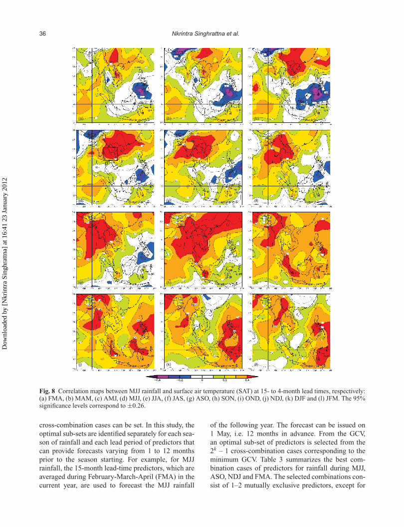
To develop a long-lead forecasting model, the sta-tistical relationships between rainfall during MJJ,ASO, NDJ and FMA and the large-scale atmo-spheric variables are developed by correlation mapswith varying lead times of the atmospheric vari-ables. Figure 8 shows examples of developed rela-tionships between pre-monsoon season (MJJ) rainfalland SAT for 12 different lead times varying from
4 to 15 months before the beginning of the pre-monsoon season in May. The solid box represents theselected region of predictor which has high correla-tion at the 95% significance level (upper and lowerbounds of +0.26 and –0.26, respectively). Statisticalrelationships from correlation maps were also devel-oped for the variables SLP, SXW and SYW and ASO,NDJ and FMA rainfall data (not shown). The signif-icant relationships of monsoon rainfall (i.e. MJJ andASO rainfall) show development with the large-scaleatmospheric variables over the study basin and thenearby seas and oceans, e.g. South China Sea, theIndian Ocean and the Pacific Ocean. The developedrelationships are found to be associated with longlead times of atmospheric variables of 8–15 monthsprior to the start of the season. This is corrobo-rated by Sahai et al. (2003) and Nicholls (1983),who presented long-lead relationships between Indiansummer monsoon rainfall and atmospheric variables,e.g. SST. The significant relationships between mon-soon (i.e. MJJ and ASO) rainfall and large-scaleatmospheric variables suggest the ability of the rain-fall forecasting models to make long-lead forecastsusing the identified atmospheric predictors, which ishardly found in any study of Thailand rainfall fore-casting (Hung et al. 2009, Singhrattna et al. 2005a,Weesakul and Lowanichchai, 2005). However, thedry-season (i.e. NDJ and FMA) rainfall gave shorterlead-time relationships with large-scale atmosphericvariables of 7–10 months. Furthermore, significantlinks are found over distant regions, e.g. Sumatraand Java (Indonesia), and northeast India, whichshows the remote influence of atmospheric circulation(Harshburger et al. 2002, Tereshchenko et al. 2002).Table 2 summarizes the identified predictors of large-scale atmospheric variables. It is also noted that thesignificant relationship between SLP and NDJ rainfallis hardly found over the region, e.g. the study basin,the Pacific Ocean and the South China Sea. Moreover,the observed rainfall data (RAIN) are included in theidentified predictors because, from the lag autocor-relation analysis (Fig. 9), the negative correlations at95% significance level are associated with a 6-monthlag (and the positive correlations – with a 12-monthlag), which indicates the ability of forecasting modelsto give long-lead forecasts using RAIN as the predic-tor. Hence, there are five identified predictors each ofthe MJJ, ASO and FMA rainfall, and four predictorsfor the NDJ rainfall.
Subsequently, an optimal combination of predic-tors is selected by cross-validated multiple regres-sion. Based on k independent predictors, the 2k – 1
Dow
nloa
ded
by [
Nkr
intr
a Si
nghr
attn
a] a
t 16:
41 2
3 Ja
nuar
y 20
12
36 Nkrintra Singhrattna et al.
(a) (b) (c)
(d) (e) (f)
(g) (h) (i)
(j) (k) (l)
Fig. 8 Correlation maps between MJJ rainfall and surface air temperature (SAT) at 15- to 4-month lead times, respectively:(a) FMA, (b) MAM, (c) AMJ, (d) MJJ, (e) JJA, (f) JAS, (g) ASO, (h) SON, (i) OND, (j) NDJ, (k) DJF and (l) JFM. The 95%significance levels correspond to ±0.26.
cross-combination cases can be set. In this study, theoptimal sub-sets are identified separately for each sea-son of rainfall and each lead period of predictors thatcan provide forecasts varying from 1 to 12 monthsprior to the season starting. For example, for MJJrainfall, the 15-month lead-time predictors, which areaveraged during February-March-April (FMA) in thecurrent year, are used to forecast the MJJ rainfall
of the following year. The forecast can be issued on1 May, i.e. 12 months in advance. From the GCV,an optimal sub-set of predictors is selected from the2k – 1 cross-combination cases corresponding to theminimum GCV. Table 3 summarizes the best com-bination cases of predictors for rainfall during MJJ,ASO, NDJ and FMA. The selected combinations con-sist of 1–2 mutually exclusive predictors, except for
Dow
nloa
ded
by [
Nkr
intr
a Si
nghr
attn
a] a
t 16:
41 2
3 Ja
nuar
y 20
12

Hydroclimate variability and long-lead forecasting of rainfall over Thailand by large-scale atmospheric variables 37
Table 2 Summary of the large-scale atmospheric pre-dictors identified from the correlation maps for seasonalrainfall during May-June-July (MJJ), August-September-October (ASO), November-December-January (NDJ) andFebruary-March-April (FMA).
Season ofrainfall
Atmosphericvariables
Spatial coverage
Latitude Longitude
MJJ SAT 20.0◦N 97.5–102.5◦ESLP 7.5–10.0◦N 102.5–107.5◦ESXW 0◦ 82.5–87.5◦ESYW 0–2.5◦N 172.5–175.0◦ERAIN 15.30–19.36◦N 98.05–100.70◦E
ASO SAT 2.5–5.0◦N 107.5–110.0◦ESLP 17.5–20.0◦N 97.5–100.0◦ESXW 10.0◦N 100.0–102.5◦ESYW 10.0◦N 95.0–97.5◦ERAIN 15.30–19.36◦N 98.05–100.70◦E
NDJ SAT 2.5–7.5◦S 97.5–102.5◦ESXW 2.5–5.0◦S 62.5–67.5◦ESYW 20.0–22.5◦N 85.0◦ERAIN 15.30–19.36◦N 98.05–100.70◦E
FMA SAT 7.5◦S 110.0–112.5◦ESLP 15.0◦N 187.5–192.5◦WSXW 17.5◦N 140.0–150.0◦ESYW 2.5◦S–2.5◦N 95.0–97.5◦ERAIN 15.30–19.36◦N 98.05–100.70◦E
SAT: surface air temperature; SLP: sea-level pressure; SXW: sur-face zonal wind; SYW: surface meridian wind; RAIN: observedrainfall over study basin.
201510Lag
50
1.0
0.5
0.0A
CF
–0.5
Fig. 9 Correlogram or lag autocorrelation (ACF) ofmonthly rainfall for 1950–2007. The dashed lines representthe correlations being significant at the 95% confidencelevel.
two combination cases for ASO rainfall correspond-ing to the 6- and 10-month forecasting lead timesthat address three predictors of SAT, SXW and SYW,and SAT, SYW and RAIN, respectively. The identi-fied sub-sets indicate that the univariate regression oflarge-scale atmospheric variables (e.g. SXW or SYW)and the multivariate regression (e.g. SYW and RAIN
or SLP and SXW) are more efficient than the univari-ate regression of observed rainfall (i.e. RAIN). Thissuggests the better performance of a fitting regres-sion and forecasting model with the incorporationof large-scale atmospheric predictors, e.g. SAT andSLP (Basson and Rooyen, 2001, Trenberth et al.2006, Sadhuram and Ramana Murthy, 2008) com-pared to developing a regression from only laggingrelationships of hydroclimatic variables, e.g. RAIN.
7.2 Forecasting evaluation
The lhf scores used to evaluate the modified k-nnmodel with the leave-one-out technique are com-puted separately for each season of rainfall, for eachyear of 1950–2007 and each forecasting lead time.Figure 10 shows plots of median lhf for seasonal rain-fall during MJJ, ASO, NDJ and FMA. A score of0.0 indicates lack of model performance in captur-ing the pdf of climatology, whereas a score greaterthan 1.0 indicates better model performance than cli-matology. The darker shading represents higher lhfscores or better model performance. From the medianlhf of 1950–2007 rainfall ensembles (Fig. 10(a)), highscores can be found corresponding to the forecastof MJJ and ASO rainfall at long lead times (e.g.7–9 months and 11 months). The successful long-lead forecasting of the modified k-nn model indi-cating higher skills than climatology (i.e. lhf scoresgreater than 1.0) was hardly found in previous stud-ies (Kulkarni, 2000, DelSole and Shukla, 2002). Themodified k-nn model also performed better than theclimatology of MJJ and ASO rainfall at short fore-casting lead times, e.g. 1–2 months (Singhrattna et al.2005a, Grantz et al. 2005). However, associated withlhf scores of less than 1.0, the forecasting perfor-mance of the model with dry-season (i.e. NDJ andFMA) rainfall decreases considerably even at shortlead times because, in terms of physical mechanism,the dry-season rainfall over the study basin is influ-enced by unstable local conditions, e.g. higher surfacetemperature and humidity, at finer time scales, e.g.hourly and daily (TMD 2007). Hence, the modifiedk-nn model, which is developed based on the relation-ships between rainfall and large-scale atmosphericvariables at seasonal time scales, performs better inmonsoon rainfall forecasting than dry-season rainfallforecasting.
To compare the prediction ability of the modi-fied k-nn model in extreme years, Fig. 10(b) and (c)present plots of median lhf for dry rainfall years (rain-fall below the 33rd percentile) and wet rainfall years
Dow
nloa
ded
by [
Nkr
intr
a Si
nghr
attn
a] a
t 16:
41 2
3 Ja
nuar
y 20
12

38 Nkrintra Singhrattna et al.
Table 3 Summary of the optimal sub-sets of predictors (•) identified from the cross-validated multiple regression for sea-sonal rainfall during (a) May-June-July (MJJ), (b) August-September-October (ASO), (c) November-December-January(NDJ) and (d) February-March-April (FMA). (SAT: surface air temperature; SLP: sea-level pressure; SXW: surface zonalwind; SYW: surface meridian wind; RAIN: observed rainfall over study basin.)
Predictor SAT SLP SXW SYW RAINSeason of predictors (forecasting lead time in month)
(a) MJJ Rainfall
FMA (12) •MAM (11) •AMJ (10) •MJJ (9) • •JJA (8) •JAS (7) •ASO (6) •SON (5) •OND (4) •NDJ (3) •DJF (2) •JFM (1) •(b) ASO RainfallMJJ (12) • •JJA (11) • •JAS (10) • • •ASO (9) • •SON (8) • •OND (7) • •NDJ (6) • • •DJF (5) •JFM (4) •FMA (3) • •MAM (2) • •AMJ (1) • •(c) NDJ Rainfall
ASO (12) •SON (11) •OND (10) •NDJ (9) • •DJF (8) •JFM (7) •FMA (6) • •MAM (5) •AMJ (4) •MJJ (3) •JJA (2) •JAS (1) •(d) FMA Rainfall
NDJ (12) •DJF (11) •JFM (10) •FMA (9) •MAM (8) •AMJ (7) •MJJ (6) •JJA (5) •JAS (4) •ASO (3) •SON (2) •OND (1) •
Dow
nloa
ded
by [
Nkr
intr
a Si
nghr
attn
a] a
t 16:
41 2
3 Ja
nuar
y 20
12

Hydroclimate variability and long-lead forecasting of rainfall over Thailand by large-scale atmospheric variables 39
MJJ
ASO
NDJ
FMA
(a)
2
4
6
8
10
12
Forecasting Lead Time (month)
MJJ
ASO
NDJ
FMA
(b)
2
4
6
8
10
12
Forecasting Lead Time (month)
0
1
2
3
MJJ
ASO
NDJ
FMA
(c)
2
4
6
8
10
12
Forecasting Lead Time (month)
Fig. 10 Median likelihood (lhf) scores for seasonal rainfall during May-June-July (MJJ), August-September-October (ASO),November-December-January (NDJ) and February-March-April (FMA) for: (a) 1950–2007, (b) dry years, and (c) wet years.
(rainfall above the 67th percentile), respectively. ForMJJ rainfall, the lhf scores of dry years are higher thanthose of wet years, especially at long lead times, e.g.9–12 months. In contrast, the modified k-nn modelshows the greater predictability of ASO rainfall inwet years than in dry years. However, the highestlhf scores (i.e. 2.0–2.5) for ASO rainfall forecast inboth dry and wet years can be found associated withthe 6-month forecasting lead time, which shows animpressive ability to forecast extreme events with along lead period. It is also noted that the better perfor-mance than climatology (i.e. lhf greater than 1.0) ofwet ASO rainfall can be observed for all 12 forecast-ing lead times. In addition, the good performance oflong-lead rainfall forecasts is obtained for dry NDJ(and short-lead forecasts for wet NDJ). For FMArainfall, the forecast of dry years shows better perfor-mance than wet years, in particular, at the forecastinglead time of 5–6 months.
Therefore, the large-scale atmospheric variablesare identified and used as predictors of the modi-fied k-nn model to forecast seasonal rainfall in thePing River Basin for 12 forecasting lead periods.The optimal combination sets of predictors that aredetermined by GCV consist of 1–2 predictors. Thiscan confirm the comparative performance of a fittingregression and forecasting model using the large-scale atmospheric predictors. Since the irrigated areaof the study basin covers 2332 km2, and the agri-culture depends on both the rainfall during the mon-soon season and the irrigated water (also based onrainfall), the ability of the modified k-nn model tomake long-lead forecasts for monsoon rainfall, e.g.7–9 months prior to the season starting, is very useful
for water resources planning and management, agri-cultural practices and cropping strategies. Moreover,the operation planning of several storage dams alongthe Ping River including the Bhumipol Dam can bedone in advance to deal with the extreme events, i.e.dry and wet episodes, and to efficiently serve thewater demands of the Ping and Chao Phraya riverbasins, consisting of 6127 and 11 000 × 106 m3
per year, respectively. The non-exceedence and excee-dence probabilities of extreme events obtained fromthe pdf of rainfall forecasting ensembles serve as atool for decision making in reservoir operation, andthe modified k-nn model shows better performance incapturing the pdf than the climatology.
8 CONCLUSION
This study enhances the understanding of local hydro-climate variability and develops statistical relation-ships between rainfall and large-scale atmosphericvariables. The land–sea temperature gradient plays akey role in strengthening or weakening the monsoonover the Upper Chao Phraya River Basin in Thailand.The amount of dry-season (November–April) rainfalldetermines the MAM temperature which is responsi-ble for setting up the land–sea temperature gradient.Higher MAM temperature tends to increase monsoon(i.e. ASO) rainfall. Due to the anomalous atmosphericvariables, the below-normal rainfall corresponds tothe El Niño phase of ENSO and, conversely, theabove-normal rainfall corresponds to the La Niñaphase.
Using the correlation maps, the large-scale atmo-spheric variables are identified as the predictors
Dow
nloa
ded
by [
Nkr
intr
a Si
nghr
attn
a] a
t 16:
41 2
3 Ja
nuar
y 20
12

40 Nkrintra Singhrattna et al.
of seasonal rainfall. The significant relationshipsbetween rainfall and large-scale atmospheric vari-ables indicate the long-lead forecasting ability offorecasting models. There are five identified predic-tors for each of MJJ, ASO and FMA rainfall, andfour identified predictors for NDJ rainfall. Based onthe cross-validated multiple regression, optimal com-binations of predictors are selected separately foreach season of rainfall and forecasting lead period.The selected combinations composed of one or twomutually exclusive predictors present the compar-ative performance of a regression and forecastingmodel by incorporation of the large-scale atmosphericvariables.
The modified k-nn model is ultimately developedto forecast rainfall at long lead times using the optimalsets of predictors. Based on lhf scores, the modifiedk-nn model shows the ability to give long-lead fore-casts of MJJ and ASO rainfall at 7–9 months leadtime. However, decreasing performance is found indry-season rainfall forecasts at both short and longlead times. The ability to forecast rainfall in dry MJJis more significant than in wet MJJ, especially at leadtimes of 9–12 months. The best performance of ASOrainfall forecast in extreme years, i.e. dry and wet, isobserved at a 6-month lead time. The long-lead fore-casting ability of the modified k-nn model for rainfallin the Ping River Basin is an impressive result that canbe applied to manage water resources and develop thelong-term plans for reservoirs.
Acknowledgements The authors would like tothank Dr Sutat Weesakul and Dr Kiyoshi Hondafor their valuable comments. The authors alsothank the Royal Irrigation Department of Thailand,the Thailand Meteorological Department andthe Department of Water Resources for providing thedata for the study. The first author is grateful to theAsian Institute of Technology, Thailand for the grad-uate fellowships, to the Department of Public Worksand Town & Country Planning for its kind supportand to Piyawat Wuttichaikitcharoen for providingsome data used in this research. The research fundingfrom CIRAD is gratefully acknowledged. Finally, theauthors would like to thank the anonymous reviewerswhose comments improved the manuscript.
REFERENCES
An, S.I., Kug, J.S., Timmermann, A., Kang, I.S. and Timm, O., 2007.The influence of ENSO on the generation of decadal variabilityin the North Pacific. Journal of Climate, 20 (4), 667–680.
Basson, M.S. and Rooyen, J.A., 2001. Practical application of prob-abilistic approaches to the management of water resourcesystems. Journal of Hydrology, 241 (1–2), 53–61.
Cañón, J., González, J. and Valdés, J., 2007. Precipitation in theColorado River basin and its low frequency associated withPDO and ENSO signal. Journal of Hydrology, 333 (2–4),252–264.
Chen, T.-C. and Yoon, J.-H. (2000) Interannual variation in Indochinasummer monsoon rainfall: possible mechanism. Journal ofClimate, 13 (11), 1979–1986.
Clark, C.O., Cole, J.E. and Webster, P.J., 2000. Indian Ocean SSTand Indian summer rainfall: predictive relationships and theirdecadal variablitiy. Journal of Climate, 13, 2503–2519.
Clark, M.P., Serreze, M.C. and McCabe, G.J., 2001. Historical effectsof El Niño and La Niña events on the seasonal evolution of themontane snowpack in the Columbia and Colorado River basins.Water Resources Research, 37 (3), 741–757.
COAPS, 2006. ENSO index according to JMA SSTA (1868 – present).http://coaps.fsu.edu/jma.shtml.
CPC (Climate Prediction Center), 2006. Cold and warmepisodes by season. http://www.cpc.ncep.noaa.gov/products/analysis_monitoring/ensostuff/ensoyears.shtml.
CPC (Climate Prediction Center), 2007. The tropical Pacific OceanSST indices. http://www.cpc.noaa.gov/data/indices.
DelSole, T. and Shukla J., 2002. Linear prediction of Indian monsoonrainfall. Journal of Climate, 15, 3645–3658.
Eldaw, A.K., Salas, J.D. and Garcia, L.A., 2003. Long-range fore-casting of the Nile River flows using climatic forcing. Journalof Applied Meteorology, 42 (7), 890–904.
ESRL (Earth System Research Laboratory), 2008. Interactive plot-ting and analysis: linear monthly/seasonal correlations. http://www.esrl.noaa.gov/psd/data/correlation.
Fasullo, J. and Webster, P.J., 2002. Hydrological signatures relatingthe Asian summer monsoon and ENSO. Journal of Climate,15(21), 3082–3095.
Gershunov, A., 1998. ENSO influence on intraseasonal extremerainfall and temperature frequencies in the contiguous UnitedStates: implications for long-range predictability. Journal ofClimate, 11 (12), 3192–3203.
Goswami, B.N., Wu, G. and Yasunari, T., 2006. The annual cycle,intraseasonal oscillation, and roadblock to seasonal predictabil-ity of the Asian summer monsoon. Journal of Climate, 19 (20),5078–5099.
Grantz, K., Rajagopalan, B., Clark, M. and Zagona, E., 2005.A technique for incorporating large-scale climate informationin basin-scale ensemble streamflow forecasts. Water ResourcesResearch, 41, W10410, doi:10.1029/2004WR003467.
Gutiérrez, F. and Dracup, J.A., 2001. An analysis of the feasibil-ity of long-range streamflow forecasting for Colombia usingEl Niño-Southern Oscillation indicators. Journal of Hydrology,246 (1–4), 181–196.
Haan, C.T., 2002. Statistical methods in hydrology, second edition.Iowa: Iowa State Press.
Hamlet, A.F., Huppert, D. and Lettenmaier, D.P., 2002. Economicvalue of long-lead streamflow forecasts for Columbia Riverhydropower. Journal of Water Resource Planning – ASCE128 (2), 91–101.
Harshburger, B., Ye, H. and Dzialoski, J., 2002. Observation evidenceof the influence of Pacific SSTs on winter precipitation andspring stream discharge in Idaho. Journal of Hydrology, 246(1–4), 157–169.
Hung, N.Q., Babel, M.S., Weesakul, S. and Tripathi, N.K., 2009.An artificial neural network model for rainfall forecasting inBangkok, Thailand. Hydrology and Earth System Sciences, 13,1413–1425.
Kalnay et al., 1996. The NCEP/NCAR 40-year reanalysis project.Bulletin of the American Meteorological Society, 77, 437–470.
Dow
nloa
ded
by [
Nkr
intr
a Si
nghr
attn
a] a
t 16:
41 2
3 Ja
nuar
y 20
12

Hydroclimate variability and long-lead forecasting of rainfall over Thailand by large-scale atmospheric variables 41
Kim, T.W., Valdés J.B.., Nijssen, B. and Roncayolo, D., 2006.Quantification of linkages between large-scale climatic pat-terns and precipitation in the Colorado River basin. Journal ofHydrology, 321 (1–4), 173–186.
Krishna Kumar, K., Soman, M.K., and Rupakumar, K. (1995)Seasonal forecasting of Indian summer monsoon rainfall:a review. Weather, 50, 449–467.
Krishnan, R., Zhang, C. and Sugi, M., 2000. Dynamics of breaks inthe Indian summer monsoon. Journal of Atmospheric Science,57 (9), 1354–1372.
Kulkarni, A., 2000. A note on the performance of IMD predic-tion model for ISMR. Annual Monsoon Workshop of IndianMeteorological Society, Pune Chapter, 20 December 2000.
Loader, C. (1999) Local regression and likelihood. New York:Springer.
Masiokas, M.H., Villalba, R., Luckman, B.H., Quesne, C.L. andAravene, J.C., 2006. Snowpack variations in the central Andesof Argentina and Chile, 1951–2005: large-scale atmosphericinfluences and implications for water resources in the region.Journal of Climate, 19 (24), 6334–6352.
Mason, S.J. and Goddard, L., 2001. Probabilistic precipitationanomalies associated with ENSO. Bulletin of the AmericanMeteorological Society, 82, 619–638.
McCabe, G.J. and Dettinger, M.D., 2002. Primary modes and pre-dictability of year-to-year snowpack variation in the westernUnited States from teleconnections with Pacific Ocean climate.Journal of Hydrometeorology, 3 (1), 13–25.
Meko, D.M. and Woodhouse, C.A., 2005. Tree-ring footprint ofjoint hydrologic drought in Sacramento and upper Coloradoriver basins, western USA. Journal of Hydrology, 308 (1–4),196–213.
Mendoza, B. et al., 2005. Historical droughts in central Mexico andtheir relation with El Niño. Journal of Applied Meteorology,44 (5), 709–716.
Nagura, M. and Konda, M., 2007. The seasonal development of anSST anomaly in the Indian Ocean and its relationship to ENSO.Journal of Climate, 20 (1), 38–52.
Nicholls, N., 1983. Predicting Indian monsoon rainfall from sea sur-face temperature in the Indonesia–north Australia area. Nature,306, 576–577.
Owosina, A., 1992. Methods for assessing the space and timevariability of ground water data. Thesis (MSc), Utah StateUniversity, Utah, USA.
Pavia, E.G., Graef, F. and Reyes, J., 2006. PDO-ENSO effectsin the climate of Mexico. Journal of Climate, 19 (24),6433–6438.
PSD (Physical Sciences Division, NOAA), 2007a. Create amonthly/seasonal mean time series from the NCEP reanalysisdata set. http://www.esrl.noaa.gov/psd/cgi-bin/data/timeseries/timeseries1.pl.
PSD (Physical Sciences Division, NOAA), 2007b. The Indian OceanSST index. http://www.esrl.noaa.gov/psd/forecasts/sstlim/timeseries/index.html.
Rajagopalan, B. and Lall, U., 1999. A k-nearest-neighbor simula-tion for daily precipitation and other weather variables. WaterResources Research, 35 (10), 3089–3101.
RID (Royal Irrigation Department), 2007. The 25 major river basinsin Thailand. http://www.rid.go.th.
Sadhuram, Y. and Ramana Murthy, T.V., 2008. Simple multipleregression model for long range forecasting of Indian summer
monsoon rainfall. Meteorology and Atmospheric Physics,99 (1–2), 17–24.
Sahai, A.K., Grimm, A.M., Satyan, V. and Pant, G.B., 2003.Long-lead prediction of Indian summer monsoon rainfallfrom global SST evolution. Climate Dynamics, 20,855–863.
Saravanan, R. and Chang, P., 2000. Interaction between tropicalAtlantic variability and El Niño-Southern Oscillation. Journalof Climate, 13 (13), 2177–2194.
Schöngart, J. and Junk, W.J., 2007. Forecasting the flood-pulse inCentral Amazonia by ENSO-indices. Journal of Hydrology, 335(1–2), 124–132.
Shrestha, A. and Kostaschuk, R., 2005. El Niño/Southern Oscillation(ENSO)-related variability in mean-monthly streamflow inNepal. Journal of Hydrology, 308 (1–4), 33–49.
Shrestha, M.L., 2000. Interannual variation of summer monsoon rain-fall over Nepal and its relation to Southern Oscillation index.Meteorolical and Atmospheric Physics, 75 (1–2), 21–28.
Silverman, D. and Dracup, J.P., 2000. Artificial neural networks andlong-range precipitation prediction in California. Journal ofApplied Meteorology, 39 (1), 57–66.
Singhrattna, N., Rajagopalan, B., Clark, M. and Kumar, K.K., 2005a.Forecasting Thailand summer monsoon rainfall. InternationalJournal of Climatology, 25 (5), 649–664.
Singhrattna, N., Rajagopalan, B., Kumar, K.K. and Clark, M., 2005b.Interannual and interdecadal variability of Thailand summermonsoon season. Journal of Climate, 18 (11), 1697–1708.
Smith, S.R. and O’Brien J.J., 2001. Regional snowfall distributionsassociated with ENSO: implications for seasonal forecasting.Bulletin of the American Meteorological Society, 82 (6), 1179–1191.
Sourza Filho, F.A. and Lall, U., 2003. Seasonal to interannualensemble streamflow forecasts for Cearra, Brazil: applicationsof a multivariate semiparametric algorithm. Water ResourcesResearch, 39 (11), doi:10.1029/2002WR001373.
Tereshchenko, I., Filonov, A., Gallesgos, A., Monzón C. andRodríguez, R., 2002. El Niño 997–98 and the hydrometeoro-logical variability of Chapala, a shallow tropical lake in Mexico.Journal of Hydrology, 264 (1–4), 133–146.
TMD (Thailand Meteorological Department), 2007. The natural dis-asters in Thailand (in Thai). http://www.tmd.go.th/info/risk.pdf.
Trenberth, K.E. et al., 2007. Observations: surface and atmosphericclimate change. New York: Cambridge University Press.
Trenberth, K.E., Moore, B., Karl, T.R. and Carlos, N., 2006.Monitoring and prediction of earth’s climate: a future perspec-tive. Journal of Climate, 19 (20), 5001–5008.
Weesakul, U. and Lowanichchai, S., 2005. Rainfall forecast for agri-cultural water allocation planning in Thailand. ThammasatInternational Journal of Science and Technology, 10 (3), 18–27.
Woodruff, S.D. et al., 1993. Comprehensive Ocean – AtmosphereData Set (COADS) Release 1a: 1980–92. Earth SystemMonitor, 4 (1), 1–8.
Wu, R. and Kirtman, B.P., 2004. Understanding the impacts of theIndian Ocean on ENSO variability in a coupled GCM. Journalof Climate, 17 (20), 4019–4031.
Zehe, E., Singh, A.K. and Bárdossy, A., 2006. Modelling of mon-soon rainfall for a mesoscale catchment in North-West IndiaII: stochastic rainfall simulations. Hydrology and Earth SystemSciences 10, 807–815.
Dow
nloa
ded
by [
Nkr
intr
a Si
nghr
attn
a] a
t 16:
41 2
3 Ja
nuar
y 20
12