Hydrodynamic Slip Boundary Condition for the Moving Contact Line

in collaboration with

Xiao-Ping Wang (Mathematics Dept, HKUST)

Ping Sheng (Physics Dept, HKUST)

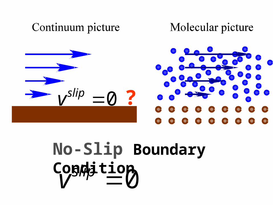
No-Slip Boundary Condition

0slipv

0slipv ?

from Navier Boundary Conditionto No-Slip Boundary Condition

: slip length, from nano- to micrometer

Practically, no slip in macroscopic flows

sslip lv

0// RlUv sslip

: shear rate at solid surface

sl

12cos s

No-Slip Boundary Condition ?

Apparent Violation seen from

the moving/slipping contact line

Infinite Energy Dissipation

(unphysical singularity)

Are you able to drink coffee?

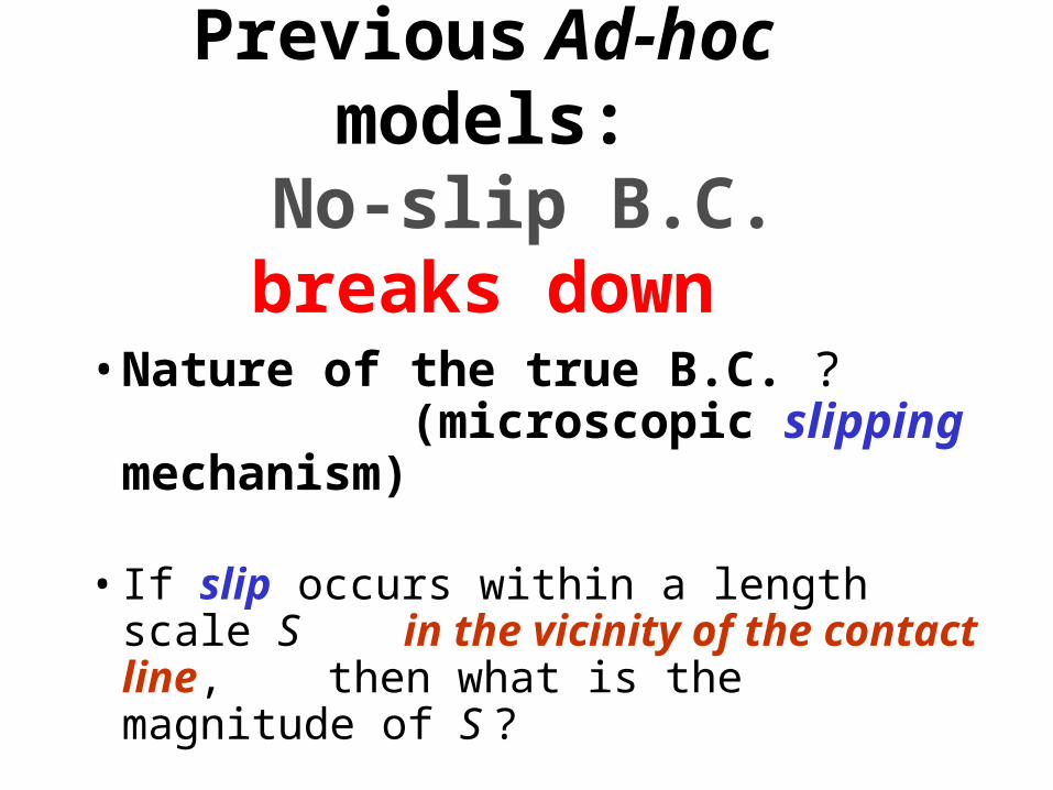
Previous Ad-hoc models: No-slip B.C. breaks down

• Nature of the true B.C. ? (microscopic slipping mechanism)

• If slip occurs within a length scale S in the vicinity of the contact line, then what is the magnitude of S ?

Molecular Dynamics Simulations

• initial state: positions and velocities• interaction potentials: accelerations• time integration: microscopic trajectories• equilibration (if necessary)• measurement: to extract various

continuum, hydrodynamic properties

• CONTINUUM DEDUCTIONCONTINUUM DEDUCTION

Molecular dynamics simulationsfor two-phase Couette flow

• Fluid-fluid molecular interactions• Wall-fluid molecular interactions• Densities (liquid)• Solid wall structure (fcc)• Temperature• System size• Speed of the moving walls

])/()/[(4 612 rrU ffff

])/()/[(4 612 rrU wfwfwfwfwf

Modified Lennard-Jones Potentials

for like molecules1fffor molecules of different species1ff

wf for wetting property of the fluid

fluid-1 fluid-2 fluid-1

dynamic configuration

static configurationssymmetric asymmetric

f-1 f-2 f-1 f-1 f-2 f-1

tangential momentum transportboundary layer

The Generalized Navier B. C.

slipx

fx vG

~

)0(~)0]([)0(~ Yzxxzzx v

)0(~~zx

fxG when the BL thickness

shrinks down to 0

viscous part non-viscous partOrigin?

int

,0,

Yzxds dx

nonviscous part

viscous part

)0()0()0(~ 0zx

Yzx

Yzx

uncompensated Young stress

Uncompensated Young Stressmissed in Navier B. C.

• Net force due to hydrodynamic deviation from static force balance (Young’s equation)

• NBC NOT capable of describing the motion of contact line

• Away from the CL, the GNBC implies NBC for single phase flows.

Continuum Hydrodynamic ModelingComponents:

• Cahn-Hilliard free energy functional retains the integrity of the interface (Ginzburg-Landau type)

• Convection-diffusion equation (conserved order parameter)

• Navier - Stokes equation (momentum transport)

• Generalized Navier Boudary Condition

)]()(2

1[ 2 fKrdFCH

)/()( 1212 42

4

1

2

1)( urf

Diffuse Fluid-Fluid InterfaceCahn-Hilliard free energy (1958)

extmv

m

gp

vvtv

])(/[

2/ Mvt

is the chemical potential.

/CHFcapillary force density

)0(~zx

slipxv

)0]()/[(

)0]([

xwfz

xz

K

v

= tangential viscous stress + uncompensated Young stress

Young’s equation recovered in the static case by integration along x

)0](/)([

)0](/[

wfzK

vt

in equilibrium, together with

0/)( wfzK

for boundary relaxation dynamics first-order generalization from

0/ vt

Comparison of MD and Continuum Hydrodynamics Results

• Most parameters determined from MD directly

• M and optimized in fitting the MD results for one configuration

• All subsequent comparisons are without adjustable parameters.

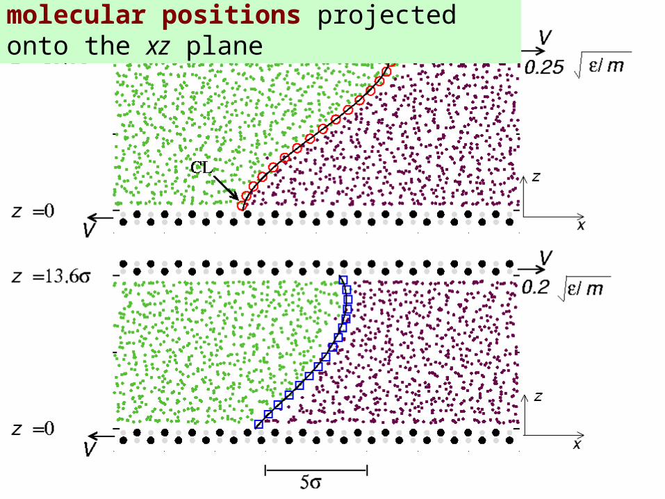
molecular positions projected onto the xz plane

Symmetric Coutte V=0.25 H=13.6

near-total slip at moving CL

1/ Vvx

no slip

symmetricCoutteV=0.25H=13.6

asymmetricCoutte V=0.20 H=13.6

profiles at different z levels

)(xvx

symmetricCoutte V=0.25 H=10.2

symmetricCoutte V=0.275 H=13.6

asymmetric Poiseuille gext=0.05 H=13.6

The boundary conditions and the parameter values are both

local properties, applicable to flows with different macroscopic/external conditions (wall speed, system size, flow type).

Summary:

• A need of the correct B.C. for moving CL.• MD simulations for the deduction of BC.• Local, continuum hydrodynamics

formulated from Cahn-Hilliard free energy, GNBC, plus general considerations.

• “Material constants” determined (measured) from MD.

• Comparisons between MD and continuum results show the validity of GNBC.

Large-Scale Simulations

• MD simulations are limited by size and velocity.

• Continuum hydrodynamic calculations can be performed with adaptive mesh (multi-scale computation by Xiao-Ping Wang).

• Moving contact-line hydrodynamics is multi-scale (interfacial thickness, slip length, and external confinement length scale).