hydrodynamics of large- scale roughness in open …
TRANSCRIPT
HYDRODYNAMICS OF LARGE-
SCALE ROUGHNESS IN OPEN
CHANNELS
A thesis submitted to Cardiff University
In candidature for the degree of
Doctor of Philosophy
by
Saad Mulahasan
Division of Civil Engineering, Cardiff School of Engineering
Cardiff University, 2016

HYDRODYNAMICS OF LARGE-SCALE
ROUGHNESS IN OPEN CHANNELS
Approved by:
PROFESSOR THORSTEN STOESSER, Advisor
Hydro-Environmental Research Centre
Cardiff School of Engineering
Cardiff University
Dr. PETER J CLEALL
Cardiff School of Engineering
Cardiff University
Date Approved: 2016

DECLARATION
This work has not been submitted in substance for any other degree or award at this
or any other university or place of learning, nor is being submitted concurrently in
candidature for any degree or other award.
Signed………………………………………………Date ……………………………
STATEMENT 1
This thesis is being submitted in partial fulfilment of the requirements for the degree
of PhD
Signed………………………………………………Date ……………………………
STATEMENT 2
This thesis is the result of my own independent work/investigation, except where
otherwise stated. Other sources are acknowledged by explicit references. The views
expressed are my own.
Signed………………………………………………Date ……………………………
STATEMENT 3
I hereby give consent for my thesis, if accepted, to be available for photocopying and
for inter-library loan, and for the title and summary to be made available to outside
organizations.
Signed………………………………………………Date ……………………………
STATEMENT 4
I hereby give consent for my thesis, if accepted, to be available for photocopying and
for inter-library loans after expiry of a bar on access previously approved by the
Academic Standards & Quality Committee.
Signed………………………………………………Date ……………………………

i
ACKNOWLEDGEMENTS
The undertaking of this thesis has been above all a great human adventure, which
would not have been possible without the support of many.
First, I would like to thank my supervisor, Professor Thorsten Stoesser who shared
his wealth of knowledge and guided me. I have been extremely lucky to have a
supervisor who cared so much about my work, and who responded to my questions
and queries so promptly.
I am very grateful to my second supervisor, Dr. Peter J Cleall for providing valuable
comments and discussions due to last three annual reviews that helped me to
improve my dissertation.
I want to thank Iraqi government for the financial support.
I would also like to thank all the members of staff and students of the Hydro
environmental Research Centre at Cardiff University for their support and guidance.
I would like to thank all staff members in research office and finance office in school
of engineering for their help due to my research period.
Thanks to all IT staff members who support my research with continuously
supplying network and helps.
Finally, I must express my gratitude to Suhailah my wife, for her continued
encouragement.

ii
SUMMARY
This thesis investigates the hydrodynamics of flow around/and or above an
obstacle(s) placed in a fully turbulent developed flow such as flow around lateral
bridge constriction, flow over bridge deck and flow over square ribs that are
characterized with free surface flow. Also this thesis examines the flow around one-
line circular cylinders placed at centre in a single open channel and floodplain edge
in a compound, open channel.
*Hydrodynamics studies of compound channels with vegetated floodplain have been
carried out by a number studies of authors in the last three decades. To enrich our
understanding of the flow resistance, comprehensive experiments are carried out
with two vegetation configurations-wholly vegetated floodplain and one-line
vegetation and then compared to smooth unvegetated compound channel. The main
result of the flow characteristics in vegetated compound channels is that spanwise
velocity profiles exhibit markedly different characters in the one-line and wholly-
vegetated configurations. Moreover, flow resistance estimation results are in
agreement with other experimental studies.
*A complementary experimental study was carried out to investigate the water
surface response in an open-channel flow through a lateral channel constriction and a
bridge opening with overtopping. The flow through the bridge openings is
characterized by very strong variation of the water surface including undular
hydraulic jumps. The results of simulation that was carried by (Kara et al. 2014,
2015) showed a reasonable agreement between measured and computed water
surface profiles for the constriction case and a fairly good was achieved for the
overtopping case.
*Evaluation of the shear layer dynamics in compound channel flows is carried out
using infrared thermography technique with two vegetation configurations - wholly
vegetated floodplain and one-line vegetation in comparison to non-vegetated
floodplains. This technique also manifests some potential as a flow visualization
technique, and leaves space for future studies and research. Results highlight that the
mixing shear layer at the interface between the main channel and the floodplain is
well captured and quantified by this novel approach.

iii
*Flume experiments of turbulent open channel flows over bed-mounted square bars
at low and intermediate submergence are carried out for six cases. Two bar spacings,
corresponding to transitional and k-type roughness, and three flow rates, are
investigated. This experimental study focused on two of the most aspects of channel
rough shallow flows: water surface profile and mean streamwise vertical velocity.
Results show that the water surface was observed to be very complex and turbulent
for the large spacing cases, and comprised a single hydraulic jump between the bars.
The streamwise position of the jump varied between the cases, with the distance of
the jump from the previous upstream bar increasing with flow rate. The free surface
was observed to be less complex in the small spacing cases, particularly for the two
higher flow rates, in which case the flow resembled a classic skimming flow. The
Darcy-Weisbach friction factor was calculated for all six cases from a simple
momentum balance, and it was shown that for a given flow rate the larger bar
spacing produces higher resistance. The result of the simulation that was carried out
by Chua et al. (2016) shows good agreement with the experiments in terms of mean
free surface position and mean streamwise velocity.
*Drag coefficient empirical equations are predicted by a number of authors for an
array of vegetation. The research aims to assess the suitability of various empirical
formulations to predict the drag coefficient of in-line vegetation. Drag coefficient
results show that varying the diameter of the rigid emergent vegetation affects
significantly flow resistance. Good agreement is generally observed with those
empirical equations.
Key Words: Flow Visualization; Infrared Thermography; Shallow Flows; Shear
layer; Image processing; Experiment; Free surface; Bridge hydrodynamics; Bridge
overtopping; Vegetation roughness, Emergent vegetation, Drag coefficient,
blockage; Compound channel, Lateral velocity profiles; Hydraulic resistance;
Hydraulic jump, Square bars.

iv
Table of Contents
ACKNOWLEDGEMENTS .......................................................................................... i
SUMMARY ................................................................................................................. ii
1 INTRODUCTION ............................................................................................... 8
1.1 BACKGROUND OF THE STUDY .............................................................. 8
1.2 VISUALIZATION MEASUREMENT TECHNIQUES ............................. 11
1.3 AIMS AND OBJECTIVES ......................................................................... 12
1.4 THESIS STRUCTURE ............................................................................... 14
2 WATER SURFACE RESPONSE TO FLOW THROUGH BRIDGE
OPENINGS ................................................................................................................ 17
2.1 INTRODUCTION ....................................................................................... 17
2.2 EXPERIMENTAL SETUP ......................................................................... 19
2.3 RESULTS AND DISCUSSIONS ............................................................... 24
2.3.1 Lateral Constriction .............................................................................. 24
2.3.2 Submerged Rectangular Bridge ........................................................... 30
2.4 CHAPTER SUMMARY ............................................................................. 37
3 MIXING LAYER DYNAMICS IN COMPOUND CHANNEL FLOWS ........ 40
3.1 INTRODUCTION ....................................................................................... 40
3.2 METHODOLOGY AND EXPERIMENTS SET UP ................................. 45
3.3 RESULTS AND DISCUSSIONS ............................................................... 51
3.3.1 Image Processing Technique................................................................ 51

v
3.3.2 Images of the Shear Layers .................................................................. 55
3.3.3 Effects of Vegetation............................................................................ 56
3.3.4 Time-averaged temperature distribution .............................................. 65
3.3.5 Confirmation of the Models ................................................................. 73
3.3.6 Properties of the Vortices ..................................................................... 74
3.4 CHAPTER SUMMARY ............................................................................. 76
4 FLOW RESISTANCE OF IN-LINE VEGETATION IN OPEN CHANNEL
FLOW ........................................................................................................................ 80
4.1 INTRODUCTION ....................................................................................... 80
4.2 FLOW RESISTANCE IN VEGETATED STREAMS ............................... 81
4.3 EXPERIMENTAL PROCEDURE .............................................................. 84
4.4 RESULTS .................................................................................................... 86
4.4.1 Water Level-Discharge Relationship ................................................... 86
4.4.2 Drag-Coefficient-Stem Reynolds Number Relationship ..................... 88
4.5 CHAPTER SUMMARY ............................................................................. 91
5 HYDRODYNAMICS OF COMPOUND CHANNELS WITH VEGETATED
FLOODPLAIN ........................................................................................................... 93
5.1 INTRODUCTION ....................................................................................... 93
5.2 THEORETICAL CONSIDERATIONS ...................................................... 97
5.3 EXPERIMENTAL METHODOLOGY AND SETUPS ........................... 101
5.4 RESULTS AND DISCUSSIONS ............................................................. 106
5.4.1 Impact of Vegetation on the Water Depth-Discharge Curve ............. 106
vi
5.4.2 Estimation of mean drag coefficients ................................................. 107
5.4.3 Spanwise distribution of streamwise velocity .................................... 110
5.5 CHAPTER SUMMARY ........................................................................... 120
6 FREE SURFACE FLOW OVER SQUARE BARS AT LOW AND
INTERMEDIATE RELATIVE SUBMERGENCE ................................................. 123
6.1 INTRODUCTION ..................................................................................... 123
6.2 EXPERIMENTAL SET-UP ...................................................................... 127
6.3 RESULTS AND DISCUSSION ............................................................... 131
6.4 CHAPTER SUMMARY ........................................................................... 149
7 SUMMARY, CONCLUSIONS AND FUTURE WORK ................................ 152
7.1 INTRODUICTON ..................................................................................... 152
7.2 SUMMARY OF RESEARCH FINDINGS ............................................... 152
7.3 CONTRIBUTIONS TO OPEN CHANNEL HYDRODYNAMICS
RESEARCH ......................................................................................................... 154
7.4 CONTRIBUTIONS TO COMPOUND OPEN CHANNEL FLOW
RESEARCH ......................................................................................................... 158
7.5 RECOMMENDATIONS FOR FUTURE RESEARCH ........................... 161
REFERENCES ......................................................................................................... 165
NOMENCLATURE ................................................................................................. 182
APPENDIXES I ....................................................................................................... 186

7
CHAPTER ONE
INTODUCTION

8
1 INTRODUCTION
1.1 BACKGROUND OF THE STUDY
River flows, flows over weirs, water waves and man-made channels convey free
surface water whose surface is exposed to the atmosphere. The study of the flow
around an obstacle(s) placed in a fully developed channel flow such as cylinders,
bridge constrictions, flows over bridge decks/ ribs, is characterized by free surface
variations which is fundamental to the understanding of the flow mechanisms for
complex two- and three dimensional geometries.
In open channel flow, the presence of a hydraulic structure such as a weir or bridge
controls the flow rate over it as well as the position of the free surface. In flood
conditions, increasing discharge may cause bridge failure due to scouring at the
sediment bed. The water level is significantly raised, existing bridges may become
fully submerged with submerged orifice flow occurring through the bridge opening
and overtopping of the bridge deck, and bridges may be damaged during flood
events. Martín V. (2002) studied the cause of failure for 143 bridges worldwide; it
was found that 49% out of 143 bridges failed due to flood events (after Kingston
(2006)). The flood of 1993 in the Midwestern US paralysed a nine state area with
flood recurrence intervals varying from 100 to 500 years. Two months after the
flood, a scour hole with a depth of 17 m was mapped near the abutment of an
interstate bridge (Parola et al. 1998). In 2009, at the Atlanta metropolitan area,
Georgia, there was extensive damage to bridge abutments and embankments due to
overtopping (Gotvald and McCallum 2010). These examples of bridge failures
highlight the importance of understanding the interaction of water flow with bridge
abutment and embankments rather than considering the bridge structure in isolation.
Knowing the maximum increase of the water level in front of the obstruction is
essential during the flood seasons in order to best design future water resources
systems and hydraulic structures. There is still limited works which investigate the
response of the water surface profile in an open channel flow through different forms
of bridge openings; there are only a few physical modelling studies reported in the
literature of flow over inundated bridges and the accompanying water surface
profiles (Merville 1995, Oliveto and Hager 2002, Sturm 2006).

9
A bridge, including deck and abutments, is considered in this study to investigate the
response of the water surface in an open-channel flow through different forms of
bridge openings.
In rough open channel flows of steep slopes with low and intermediate submergence
such as steep slope mountain streams, the free surface profile carries the signature of
the bed roughness and flow regime while it affects the turbulent flow structures and
bed forms; and individual hydraulic jumps may be observed. There is no standard
analytical expression of the flow resistance equation for the determination of the
mean flow velocity for turbulent rough open channel flows making the application of
the flow resistance equation challenging for specialists. Numerous friction factor
equations were derived relative to parameters such as roughness spacing, relative
submergence, and bed material concentration, (Bathurst 1978, Bray 1979, Hey 1979,
Thompson and Campbell 1979, Bathurst et al. 1981, Bathurst 1985, Bathurst 2002,
Pagliara and Chiavaccini 2006, Rickenmann and Recking 2011). Knowing the
parameters of influence helps researchers and practitioners in solving hydraulic
engineering problems relative to bed slopes, water depths, submergence ratios, and
roughness concentrations. There are limited works investigating flow resistance due
to large-scale roughness at steep bed slopes of low relative submergence. In this
research, the hydrodynamics of shallow flows that are strongly influenced by water
surface deformation, and to quantify the effect of roughness spacing and relative
submergence on hydraulic resistance in such flows is displayed.
When the water surface of the river flow just reaches its banks, the discharge flowing
through the river is called bank full discharge. If the flow exceeds the main channel
capacity, the water will overflow the banks and will immerse the floodplains. In this
case the river capacity decreases due to the generation of shear layers and the free
surface of water is controlled by the density, distribution and configuration of the
vegetation elements on the floodplain. Large scale horizontal coherent structures
generated near the interface between the main channel and the floodplain of
compound channels have been observed with different techniques by a number of
authors (Tamai et al. 1986, Tominaga and Nezu 1991, Nezu and Onitsuka 2001, van
Prooijen et al. 2005, Rummel et al. 2006, White and Nepf 2007, Nezu and Sanjou
2008, Stocchino and Brocchini 2010). These coherent structures (shear layers) are

10
influenced by the density of the vegetation elements and their configurations on the
floodplain. To better understand the above phenomenon a novel approach of
visualization technique can be used. In this research, a thermal camera SC640 and
heat tracer (hot water) is used to track the coherent structures at the water surface at
the interface between the main channel and the floodplain in the compound channel
flow.
Open channel flow through a one-line array of vertically-oriented circular rods of
varying diameters still comprises limited works (Sun and Shiono 2009, Terrier et al.
2010, Terrier et al. 2011, Shiono et al. 2012, Miyab et al. 2015), particularly with
regards to drag coefficient calculations. Drag coefficient is calculated in terms of
emergent vegetation from equalling gravity force to drag force (Petryk and
Bosmajian 1975). A new idea was used to compare the drag coefficient results from
one-line vegetation to drag coefficient from an array of vegetation elements as
proposed by a number of researchers. In this research, drag coefficients are
compared to a number of expressions that have been proposed for an array of
emergent rigid vegetation cylindrical cylinders.
The presence of vegetation on the edge of the floodplain reduces the section capacity
of the river and its floodplain, and makes the interaction between the main channel
and the floodplain complex. Some common patterns of vegetation that is growing at
the edge of UK Rivers are straight lines, such as the River Dove at Dovedale, the
River Dove at Milldale, and the River Severn at Ironbridge Gorge. Flooding in these
areas usually arises from water overtopping the banks of streams. Flow structure of
water through a one-line array and fully vegetation distribution of vertically-oriented
circular cylinders placed along the edge of the floodplain adjacent to the main
channel, and on the entire width of the floodplain in a compound channel have been
considered by a number of authors (Tominaga and Nezu 1991, van Prooijen et al.
2005, Yang et al. 2007, Sun and Shiono 2009, Vermaas et al. 2011, Aberle and
Järvelä 2013). In this research vegetation elements are modelled by emergent rigid
wooden rods of circular cross-section. For the vegetated cases the effect of
vegetation density is investigated, and in all cases three flow rates were tested. The
effect of vegetation density and distribution on the floodplain on the rating curve, the
drag coefficients and the stream-wise velocity distribution in an asymmetric

11
compound channel is investigated experimentally. Additional focus is placed upon
the importance of interfacial shear stress in drag coefficient calculations.
1.2 VISUALIZATION MEASUREMENT TECHNIQUES
Visualization of water flow through vegetation elements is mainly carried out by
different techniques such as adding different materials to the flow and then using
optical imaging technique to track the motion of the flow. In such case, the tracer
motion is measured instead of the flow itself considering the tracer to be passive.
Rhodamine dye tracer can be tracked visually, and can be used for measuring the
surface velocity of the flow. However, there are increasing concerns over the use of
dyes that can cause environmental impacts such as the colour and the toxic
properties of the dyes (Chequer et al. 2013).
Over the years, significant improvements and developments in visualization
techniques have been performed not only resulting in higher accuracy and quality of
the obtained data, but also with the evolution of powerful new techniques with new
abilities and features, benefiting from the great development of technology in other
areas of knowledge. Flow visualization techniques such as digital cameras, laser
based methods (particle image velocimetry (PIV)/ particle tracking velocimetry
(PTV), laser induced fluorescence (LIF), laser Doppler anemometer (LDA), and
infrared thermography techniques (IF) have been developed in the last three decades.
Thermal cameras have been developed and widely propagated in the world since the
mid- 1990s.
Infrared thermography is a technique for detecting and measuring the energy that
radiates through the surface, not the temperature of the object itself. Thermal
cameras with special lens are used to detect, measure and collect the radiated thermal
energy and then convert to signals that can be processed to obtain the image with a
colour code.
Infrared thermography techniques (IR) may be used in different parts of water
science applications such as water resources, hydraulics, hydrology, fluid dynamics,
and soil and water preservation.
One of the choices with thermography techniques is that hot water is applied as heat
tracer and is then used for visualization. Using thermography technique makes it

12
possible to detect more information about the flow crisis such as coherent structures
(vortices) at the water surface and details of the flow can be extracted. The use of IR
thermography technique for flow measurements has not been extensively explored
yet, and its capabilities have yet to be studied.
Recording the spatial state of the free surface profile of water requires various
accumulations of sensors. Instead of these sensors, a particle image velocimetry
(PIV) is used that is capable of obtaining qualitative and quantitative information
such as velocity fields at any plane of shallow flows and not in a point as with ADV.
A PIV provides data measuring of flow velocities that vary in both time and space.
In addition, this technique can also be used as a non-intrusive visualization device
which make it possible to detect more information about the flow such as turbulent
coherent structures (eddies), and can be used to track the water surface profile. A
PIV system mainly consists of CCD camera, and flash stroboscope for illumination.
Seeding particles are added to the flow and illuminated by the halogen lamps.
The understanding of the free surface response of water flowing in steep ribbed
flumes remains limited; mainly, the impact of (roughness spacing, λ, to roughness
height, k) i.e. λ/k ratio, and (water depth, H, to roughness height, k) submergence
ratio, H/k on the water surface profile. Applying these visualization techniques (IR
thermography and PIV), various flow phenomena can be visualized and deeply
studied and then unclear aspects of their behaviour can be better explained.
The visualization techniques used in this research are thermal camera (SC 640) to
report and visualize the free surface flow at the interface between the vegetated or
the non-vegetated floodplain and the main channel in a compound channel flow,
while a particle image velocimetry (PIV) is used with flow above the ribbed single
channel to monitor the free surface profiles flowing over a ribbed flume at steep
slopes; a large number of captured video images are recorded in which seeding
particles are used as tracer.
1.3 AIMS AND OBJECTIVES
The scientific research objectives of the experiments with steady uniform flow are as
follows:

13
a) For rough beds (Friction factor, and water surface dynamics)
Identifying flow resistance for transverse roughness elements and compare it
with Bathurst (1981 and 1983)’s data.
Qualification of the effect of roughness spacing, λ/k, and relative
submergence, h/k, on hydraulic resistance in shallow flows.
Describing, for a fixed roughness element’s height, the impact of steep bed
slope and roughness spacing (pitch to pitch) influence on the free surface
deformation of the flow.
Investigate whether the water surface profile in a steep slope ribbed flume
can be simulated numerically.
Understanding of the mean flow characteristics for flow over square bars at
low and intermediate submergence.
b) For bridge constrictions
Investigation of the effect of lateral channel constriction and a submerged
bridge on the water surface profile.
Understanding of the mean flow characteristics for an inundated bridge.
c) For a compound channel flow
Investigate use of infrared thermography technique to capture thermal shear
layers generated at the interface between main channel and floodplain.
d) For a one-line vegetation in single open channel flows
Quantification of the drag coefficient of one-line vegetation and assessment
of the empirical expressions’ reliability for the prediction of the drag
coefficient.
Clarification of the influence of the bed slope on the rating curves of a one-
line of vertically-oriented circular rods of varying diameters.
e) For one-line vegetation in compound open channel flows placed at the interface
between the main channel and the floodplain and wholly vegetated floodplain cases

14
Investigation of the effect of vegetation density and vegetation distribution on
the rating curve, drag coefficients and lateral velocity profiles in a compound
channel at uniform flow conditions in comparison to non-vegetated
floodplain case.
Identification of the bulk changes in drag coefficient around a one-line of
vertically oriented circular rods of varying diameters when moved from the
centre of a symmetrical open channel of simple cross-section to the
floodplain edge of a symmetric compound channel flow.
1.4 THESIS STRUCTURE
The experimental study of this research is structured as follows:
Chapter 1 presents an introduction to background of the research subject areas,
visualization techniques, aim and objectives and the thesis structure.
Chapter 2 describes water surface response to flow through bridge openings. Two
bridge forms were considered as lateral constriction and submerged deck. This
chapter mainly focuses on flow dynamics through a submerged bridge opening with
overtopping. This experimental study provides a useful contribution to overtopping
case and then simulated numerically by Kara et al. (2014, 2015) which revealed the
complex nature of the flow around the bridge.
Chapter 3 presents the dynamics of shear layers at the interface between the main
channel and the floodplain in a compound channel flow. Image processing
techniques is used to extract such shear layers to state the dynamics of mixing shear
layers. Thermal snapshots are analysed in visualizing these shear layers. In addition,
two kinds of vortices are specified as shear layer vortices and von Karman street
vortices which enrich specialists to characterise fluid dynamics of flow through
cylinders.
Chapter 4 clarifies experimentally hydrodynamics of one-line of vertically-oriented
circular rods of varying diameters placed at regular spacing along the mid-width of
the single open channel flow. This study focuses on drag coefficient calculations
based on Petryk and Bosmajian’s equation.

15
Chapter 5 investigates the effect of vegetation density and vegetation distribution on
the rating curve, drag coefficients and lateral velocity profiles in a compound
channel flow with a vegetated floodplain at uniform flow conditions.
Chapter 6 presents the friction factor results of the ribbed steep slope open channel
flows. The water surface profiles of ribbed steep slope open channel flows are
presented and discussed. Vertical velocity profiles at different vertical sections are
examined. Finally, the effects of roughness spacing and relative submergence on
hydraulic resistance in shallow flows are simulated by Chua et al. (2016) to reveal
explicit contributions to the overall momentum balance due to form-induced and
turbulent stresses and the pressure drag is also quantified.
Chapter 7 summarises the research findings, conclusions and provides ideas for
future research.

16
CHAPTER TWO
WATER SURFACE RESPONSE TO FLOW
THROUGH BRIDGE OPENINGS

17
2 WATER SURFACE RESPONSE TO FLOW THROUGH BRIDGE
OPENINGS
2.1 INTRODUCTION
The presence of a bridge in a river triggers a highly turbulent flow field including 3D
complex coherent structures, e.g. (Koken and Constantinescu 2009) around the
structure. These turbulence structures are highly energetic and possess high sediment
entrainment capacity, which increases scouring around the bridge foundation, and
consequently lead to structural stability problems. During extreme hydrological
events, existing bridges may become fully submerged with submerged orifice flow
occurring through the bridge opening and weir flow over the bridge deck. Most
bridges were not designed for such flow conditions. In 1994, tropical storm Alberto
dumped as much as 71 cm of rainfall over widespread areas of Georgia (USA),
which resulted in damage to more than 500 bridges. The primary cause of damage to
bridges was scour around abutments and approach embankments accompanied by
bridge overtopping in many cases. The flood of 1993 in the Midwestern US
paralysed a nine state area with flood recurrence intervals varying from 100 to 500
years. Two months after the flood, a scour hole with a depth of 17 m was mapped
near the abutment of an interstate bridge on the Missouri River (Parola et al. 1998).
Epic flooding with the flood recurrence interval in excess of 500 years occurred in
Georgia in 2009 in the Atlanta metropolitan area with extensive damage to bridge
abutments and embankments due to overtopping (Gotvald and McCallum 2010).
These examples of bridge abutment and embankment failures highlight the need for
additional research in this area. Currently, no formula for abutment scour is widely
applicable because of difficulties in understanding the complicated hydrodynamics
that lead to scouring near bridge abutments. A submerged bridge, including deck and
abutments, is a significant obstacle to the flow, creating a backwater effect upstream
of the bridge and a distinct and strongly varying water surface profile over the bridge
deck and immediately downstream. Most studies in the literature examined
experimentally the flow characteristics of free surface flow through the bridge
opening, including complex 3D coherent structures and scouring mechanisms around
abutments (Merville 1995, Oliveto and Hager 2002, Sturm 2006) and numerically
18
(Biglari and Sturm 1998, Chrisohoides et al. 2003, Paik et al. 2004, Nagata et al.
2005, Paik and Sotiropoulos 2005, Koken and Constantinescu 2008, Koken and
Constantinescu 2009, Teruzzi et al. 2009, Koken and Constantinescu 2011).
However, there are only few studies reported in the literature on flow over inundated
bridges and the accompanying water surface profiles. Picek et al. (2007) conducted
experiments to derive equations for backwater and discharge for flows through
partially or fully submerged rectangular bridge decks. Malavasi and Guadagnini
(2003) carried out experiments to examine the hydrodynamic loading on a bridge
deck having a rectangular cross-section for different submergence levels and deck
Froude numbers. The experimental data were used to analyse the relationship
between force coefficients, the deck Froude number and geometrical parameters.
They extended their experimental studies to analyse mean force coefficients and
vortex shedding frequencies for various flow conditions due to different elevations
of the deck above the channel bottom (Malavasi and Guadagnini 2007). Guo et al.
(2009) investigated hydrodynamic loading on an inundated bridge and the flow field
around it. An experiment was conducted for a six-girder bridge deck model and the
experimental data were used to validate complementary numerical simulations. In
the experiments, the PIV technique was used to obtain velocity distributions. The
numerical data were analysed for different scaling factors to determine the effects of
scaling on hydrodynamic loading. Lee et al. (2010) focused on water surface profiles
resulting from flow around different bridge structures. They investigated three cases:
a cylindrical pier, a deck, and a bridge (i.e. cylindrical pier and deck). Overtopping
flow was considered only for the deck and bridge cases. In the experiment, the PIV
method was used to measure the velocity. A 3D Reynolds-Averaged Navier Stokes
(RANS) model with k-ε turbulence closure was used to simulate all the cases. The
volume of fluid method was utilized for free surface modelling. Finally, comparisons
of velocity distributions and water surface levels obtained from experiments and
simulations showed that the model estimates velocity distributions very well.
However, the model underestimates the water level rise around the structure due to
the inability of the k-ε turbulence model to represent such a complex flow having
significant streamline curvature and body force effects. The key objectives of this
study are (1) to contribute to existing literature in understanding the water surface

19
response to the complex flow around a lateral channel constriction and a submerged
bridge, (2) to quantify the mean and instantaneous flow through a bridge opening
with overtopping, and (3) to elucidate the complex three-dimensional hydrodynamics
and discuss their potential effects on the local scour mechanism. A complementary
experimental study is reported which demonstrates the details of the water surface
deformation and then its turbulence characteristics was simulated numerically by
(Kara et al. 2015) to validate the LES.
2.2 EXPERIMENTAL SETUP
The physical model experiments were carried out in Cardiff University’s hydraulics
laboratory in a 10 m long, 0.30 m wide tilting flume with a bed slope of 1/2000 (see
Fig. 2.1). Two bridge constrictions were chosen as sidewall abutments and
submerged rectangular bridge. The lateral constriction cases were L = 29 cm long
and B = 15 cm wide which gave a contraction ratio (B/W) of 0.5, L = 20 cm long
and B = 15.5 cm wide which gave a contraction ratio (B/W) of 0.516 and L = 9.0 cm
long and B = 9.0 cm wide which gave a contraction ratio (B/W) of 0.30. The
laboratory setup of the sidewall abutment of L = 29 cm long and B = 15 cm wide
(the LES domains and experimental) are presented in Figures 2.2 and 2.3,
respectively. In the LES drawing, all dimensions are normalized with the
length/width of the abutment, L (Kara et al. 2014).
Figure 2.1: Schematic diagram of the flume of 30 cm width.
Before inserting bridge structures into the flume, uniform flow conditions were
established for different flow cases (Fig. 2.4).

20
Figure 2.2: Computational setup for the LES of the lateral constriction (Kara et al.
2014).
For the lateral constriction case of L = 29 cm long and B = 15 cm wide the
discharge was chosen as 𝑄 = 4.6 l s-1
for which the uniform flow depth was 𝐻 = 6.4
cm. This resulted in a bulk velocity of 𝑈𝑏 = 0.24 m s-1
and a mean shear velocity of
𝑢∗ = 0.015 m s-1
. The Reynolds number based on 𝑈𝑏 and four times the hydraulic
radius, R was Re = 42,730 and the Froude number was Fr = 0.30. Point locations of
water level measurements for the lateral constriction model along the lines A, B, C,
D and a, b, c, d, and e are as shown in Fig. 2.3. For the other lateral constriction
models point locations of water level measurements were carried out at mid width
between the lateral constriction and the flume sidewall in the same manner as with
the first model. Three flow rates of 2.0 l s-1
, 3.0 l s-1
and 4.0 l s-1
were tested with
these two lateral constriction models.
Figure 2.3: Schematic diagram showing locations of water level measurements for
the lateral constriction model along the lines A, B, C, D, a, b, c, d and e. (All the
dimensions are in centimetres).

21
Figure 2.4: Water depth- discharge relationship.
For the overtopping case, the model bridge consisting of a square abutment with
length of 𝐿 = 10 cm, width of 9 cm, and height of ℎ𝑎 = 5.0 cm and a rectangular
bridge deck of thickness of ℎ𝑑 = 2.4 cm, which extended across the channel (see
Fig. 2.5).
Figure 2.5: A physical bridge model for water surface measurements.
The geometric contraction ratio of bridge opening width to channel width was 0.70.
The model bridge is an idealized version of the Towaliga River Bridge near Macon,
Georgia. Before inserting the bridge model into the flume, the stage-discharge
relationship for uniform flow was established (Fig. 2.4), for which the flow depth

22
was controlled via a weir at the downstream end. With the bridge in place, the water
backed up and caused an increase of water depth upstream of the bridge. The
discharges, chosen are as 𝑄 = 7.0 l s-1
, 8.5 l s-1
, 12.0 l s-1
and 15.0 l s-1
correspond to
an extreme flood events and the corresponding uniform flow depths were H = 7.98
cm, H = 9.2 cm, H = 9.93 cm and 11.53 cm. For comparison purposes with the
numerical approach the flow rate 8.5 l s-1
was chosen this resulted in a bulk velocity
of 𝑈𝑏 = 0.31 m s-1
and a mean shear velocity of 𝑢∗ = 0.017 m s-1
. The Reynolds
number based on 𝑈𝑏 and four times the hydraulic radius was Re = 69, 800, and the
Froude number of the uniform flow was Fr = 0.32. In the experiment, detailed water
surface profiles were measured using a point gauge. Point locations of water level
measurements for the submerged rectangular bridge model for the 8.5 l s-1
were
carried out along the lines A, B and a, b, c, d and e are shown in Fig. 2.6 while for
the other flow rates (7.0 l s-1
, 12.0 l s-1
and 15.0 l s-1
) water surface profiles were
measured just along the mid width of the flume over the bridge model. Fig. 2.7
shows the laboratory and numerical setups for the 8.5 l s-1
, In the LES drawing all
dimensions are normalized with the length/width of the abutment, L (Kara et al.
2015).
Figure 2.6: Schematic diagram showing locations of water level measurements for
the submerged rectangular bridge model along the lines A, B (top) and a, b, c, d and
e (bottom).

23
Figure 2.7: Computational setup for the LES of the model bridge (Kara et al. 2015).
Flow rates for the overtopping bridge model were measured by separating the flow
into weir flow and an orifice flow. Point velocity measurements were carried out
using Nixon probe velocimetry. For the broad crested weir, velocity measurements
were carried out at six sections at two positions along each section at 0.2h and 0.8h
with an averaged velocity is Uavg. = (0.2Hs+0.8Hs)/2, where Hs is the flow depth
over the bridge deck. For the orifice flow, velocity measurements were carried out at
two positions, 0.2Ho and 0.8Ho for the four selected sections as shown in Fig. 2.8,
where Ho is the flow depth of the orifice flow opening. The rotary of the probe was
positioned at the downstream edge of the bridge model at these two positions.
Figure 2.8: Point velocity measurements of separating the flow to an orifice flow and
broad crested weir flow.
If the flow occurs along the entire bridge with the water level upstream the bridge
below the upper edge of the bridge deck, the flow is called the full-flowing-orifice
type of flow. Only one case was considered as full flowing orifice flow with a flow
rate of 4.5 l s-1
. Water level measurements were carried out along the mid width

24
upstream and downstream the bridge opening at distances as with the overtopping
case studies.
2.3 RESULTS AND DISCUSSIONS
Figure 2.9 presents the water surface elevation measurement locations for the two
cases along which LES carried out by Kara et al. (2015) and experimental data
which will be compared . Profiles denoted with a capital letter represent longitudinal
profiles, and profiles denoted with a small letter are cross-sectional profiles.
Figure 2.9: Water surface elevation measurement locations of the lateral constriction
(top) and model bridge cases (Kara et al. 2014).
2.3.1 Lateral Constriction
The water surface profiles in longitudinal profiles A-D are presented in Figure 2.10.
The water surface elevations are normalized with H. Overall, the profiles obtained
from the LES show reasonable agreement with the experimental data. The water is
backed up quite significantly upstream of the structure and the LES predicts this
quite well. A bit upstream of the structure (indicated by the dashed lines) the flow

25
starts to accelerate and the water surface drops rapidly and significantly. The flow
creates a very distinct local dip in the area of local recirculation as a result of flow
separation at the leading edge of the constriction. The water surface recovers
markedly approximately half way through the constriction in form of a standing
wave. The simulation is reproducing this fairly well away from the structure
(Profiles C and D), however very close (e.g. Profile A) the agreement is not so good.
This can be attributed to the lack of mesh resolution of the simulation and apparently
the LES cannot resolve the steep gradients well enough. Near the end of the
constriction, the water surface drops further quite significantly. The flow
downstream of the constriction is subjected to a large very shallow recirculation zone
just behind the abutment, which contracts and accelerates the flow. The LES
reproduces this part of the water surface response quite well.
Figure 2.11 presents cross-sectional water surface profiles immediately before
(profile a-b) and after (profile c-e) the constriction as obtained from experiment and
LES. The match between simulation and experiment upstream of the constriction is
quite satisfying and the lateral gradient is reproduced very well. This gradient
reflects the acceleration of the fluid in the non-constricted area due to the presence of
a recirculation zone just up-stream of the constriction. The gradient of water surface
increases closer to the constriction. The cross-sectional profiles downstream of the
constriction exhibit a very significant jump in the water surface. The recirculation
zone downstream of the constriction is significantly lower elevation than the rest of
the channel. The water that rushes out of the constricted area has a significant
amount of stream wise momentum prohibiting the filling of the recirculation zone
with fluid. The features described in conjunction with Figures 2.10 and 2.11 can be
observed in Figure 2.12, depicting a photograph looking from downstream of the
constriction. Aforementioned water surface features are highlighted in the
photograph and accordingly in the visualized large-eddy simulation. The local
depression at the leading edge of the constriction is marked with a black arrow; the
recovery of the depressed water in the constriction is highlighted by yellow arrows
and the recirculation zone is denoted RZ. All these features are predicted well
qualitatively by the LES. Moreover, there is a small ridge in the water surface
between the depressed recirculation zone and the elevated flow out of the

26
constriction, which is not picked up in the measurements (see profiles c, d, e) but is
clearly visible in the photograph and in the simulation (highlighted by a thin orange
line).
Figure 2.10: Longitudinal water surface profiles (dots represent the experimental
data. Solid black line represents fine grid LES result) (Kara et al. 2014).

27
Figure 2.11: Water surface profile comparisons for cross sections (dots represent the
experimental data. Solid black lines represent LES results) (Kara et al. 2014).

28
The flow in the constriction changes criticality and it is supercritical for
approximately 6-8L downstream of the constriction before the flow returns to
subcritical in a weak hydraulic jump. In the LES this happened very close to the
domain exit and posed a challenging task in terms of numerical stability.
Free surface profiles along the mid width of the lateral constriction and the flume
sidewall for the other lateral constrictions (L = 20 cm long and B = 15.5 cm wide
and L = 9.0 cm long and B = 9.0 cm wide) for the three flow rates 2.0 l s-1
, 3.0 l s-1
and 4.0 l s-1
were shown in Figs. 2.13 an d 2.14 respectively. Combining these two
lateral constrictions in a one drawing was shown in Fig. 2.15. The most important
features of these water surface profiles are a marked drop of the water surface,
increasing the blockage ratio influences the water surface meandering exhibiting
wavy motion to the uniform flow condition and results in complex water surface
profiles and for large blockage the height of local up swell locates a bit upstream of
the structure decreased with the increasing depth of water.
Figure 2.12: Snapshots of the instantaneous water surface from experiment and as
predicted by the LES (Kara et al. 2014).

29
Figure 2.13: Free water surface profiles in presence of a lateral constriction of
dimensions 9 cm X 9 cm.
Figure 2.14: Free water surface profiles in presence of a lateral constriction of
dimensions 20 cm X 15.5 cm.

30
Figure 2.15: Free water surface profiles in presence of the lateral constrictions of
dimensions 9 cm X 9 cm and 20 cm X 15.5 cm.
2.3.2 Submerged Rectangular Bridge
Figure 2.16 (top) presents an overall three-dimensional view of the time-averaged
water surface of this flow as predicted by a numerical simulation (Kara et al. 2015).
Also plotted (bottom right) is a close up photograph of the corresponding flow over
the bridge in the experiment. The flow accelerates over the bridge causing a marked
drop of the water surface. The flow plunges downstream of the bridge, which results
in a standing wave or an Undular hydraulic jump. Downstream of the standing wave
the flow recovers gradually, exhibiting wavy motion, to the uniform flow condition.
In general, Fig. 2.16 shows very good qualitative agreement between the numerical
results and the conditions observed in the laboratory experiment.

31
Figure 2.16: Simulated water surface (top), measurement locations (bottom left) and
close-up photograph of the laboratory experiment (bottom right).
A more quantitative assessment of the predictive capabilities of the simulation
results is provided in Figs 2.17 and 2.18, which depict measured (dots) and
simulated (lines) longitudinal (Fig. 2.17) and cross-sectional profiles (Fig. 2.18) of
the water surface. The simulated longitudinal profiles (Fig. 2.17) along A and B (see
the sketch in the lower left of Fig. 2.16) are in very good agreement with the
observed data. There is a small, but consistent overestimation of the water surface
elevation upstream of the bridge. The reason for this discrepancy is that the height of
the bridge deck in the simulation was chosen to be exactly 50% of the depth of water
underneath the deck. The height of the bridge deck in the experiment was 48% of the
depth of water underneath it. There is some discrepancy between numerical
prediction and measurement in the vicinity of the standing wave, an area that is
highly turbulent and where accurate water surface measurements using a point-gauge
are difficult to achieve. Figure 2.18 presents measured and simulated cross-sectional
water surface profiles at selected locations (a–e, see Fig. 2.16). Upstream and on the
bridge (profiles a and b) the numerically predicted profiles are slightly higher than
the measured ones, whereas numerically predicted profiles c, d and e are in very
good agreement with the measurements.

32
Figure 2.17: Longitudinal water surface profiles along two locations, which are
channel centre line (profile A) and one-third of the channel width (profile B) at the
abutment face (Kara et al. 2015).
Figure 2.18: Cross-stream water surface profiles along six locations (profiles a–e)
looking upstream (Kara et al. 2015).
A quantitative view of the flow is provided with the help of Fig. 2.19, in which the
time-averaged stream-wise velocity together with streamlines in three longitudinal
planes are plotted. The time-averaged flow over the bridge is subdivided into two
portions: 74.4% of the discharge is forced underneath the bridge deck as submerged
orifice flow, whilst the remaining 25.6% discharges over the deck as a weir flow.
The deck acts similarly to a broad-crested weir and the critical depth of the portion
over the deck is yc = (q2/g)
1/3 = 1.73 cm, which is attained at 0.93L, i.e. very close to
the trailing edge of the deck. The flow plunges into the downstream area as
supercritical flow, and undergoes an ‘Undular’ hydraulic jump. A vertical
recirculation zone forms downstream of the abutment as depicted in Fig. 2.19a. On
the side of the abutment the standing wave is not as steep as in the middle of the

33
channel, a feature that was also observed in the experiment. At y/W = 0.33 the
separation vortex over the deck interacts with the lateral flow separation and
recirculation from the abutment generating a vortex core at x/W= 0.7 and a saddle
point underneath (Fig. 2.19b). At y/W = 0.67 (Fig. 2.19c) the submerged orifice
flow features stream-wise velocities up to almost three times the bulk velocity,
which is due to the lateral and vertical contraction of the flow not only by the
abutment and deck but also by the vertical and horizontal recirculation zones of the
separated flow.
Figure 2.19: Time-averaged velocity contours together with streamlines of the flow
in three selected longitudinal-sections: (a) y/W = 0.17; (b) y/W = 0.33; (c) y/W = 0.67
(Kara et al. 2015).
34
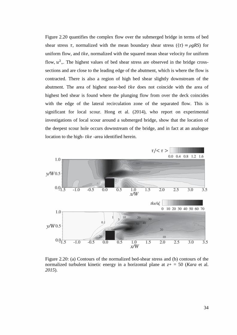
Figure 2.20 quantifies the complex flow over the submerged bridge in terms of bed
shear stress 𝜏, normalized with the mean boundary shear stress (⟨𝜏⟩ = ρgRS) for
uniform flow, and 𝑡𝑘𝑒, normalized with the squared mean shear velocity for uniform
flow, 𝑢2∗. The highest values of bed shear stress are observed in the bridge cross-
sections and are close to the leading edge of the abutment, which is where the flow is
contracted. There is also a region of high bed shear slightly downstream of the
abutment. The area of highest near-bed 𝑡𝑘𝑒 does not coincide with the area of
highest bed shear is found where the plunging flow from over the deck coincides
with the edge of the lateral recirculation zone of the separated flow. This is
significant for local scour. Hong et al. (2014), who report on experimental
investigations of local scour around a submerged bridge, show that the location of
the deepest scour hole occurs downstream of the bridge, and in fact at an analogue
location to the high- 𝑡𝑘𝑒 -area identified herein.
Figure 2.20: (a) Contours of the normalized bed-shear stress and (b) contours of the
normalized turbulent kinetic energy in a horizontal plane at z+ = 50 (Kara et al.
2015).

35
The measurements of water surface profiles through entirely submerged bridge deck
of a rectangular shape was carried out for all the flow rates of 7.0 l s-1
, 8.5 l s-1
, 12.0 l
s-1
and 15.0 l s-1
showed that the shape of profiles are complex.
The most features of the water surface profiles are the height of local upswell locates
a bit upstream of the structure decreased with the increasing depth of water above the
bridge deck and Undular hydraulic jumps were observed in all the flow rates. Strong
hydraulic jumps were shown in high flow rates downstream of the abutment as
depicted in Fig. 2.21.
Figure 2.21: Water surface profiles of the flow over the submerged bridge deck.
The time-averaged flow over the bridge as mentioned earlier is subdivided into two
portions: a submerged orifice flow and a broad crested weir flow was explained in
Fig. 2.22 shows 49.9%, 38.9%, 25.6% and 21.9% for the flow rates 15.0 l s-1
, 12.0 l
s-1
, 8.5 l s-1
and 7.0 l s-1
is running as a weir flow respectively.
Water surface profile for the full-flowing-orifice type of flow was represented by the
full line with circles as shown in Fig. 2.23.

36
Figure 2.22: Percent submergence ratio versus discharge relationship.
Figure 2.23: Schematic picture of observed water-surface profile of flow through the
full-flowing-orifice type of flow.

37
2.4 CHAPTER SUMMARY
This chapter explains experimentally and then compares numerically the calculations
of the longitudinal free surface profiles and the cross sectional profiles for two case
studies of bridge constrictions such as lateral constriction and bridge overtopping.
For the purpose of comparison the numerical approach with the experimental data,
two flow rates were considered from the rating curve for the case studies. For the
lateral constriction case the discharge was 𝑄 = 4.6 l s-1
for which the uniform flow
depth was 𝐻 = 6.4 cm. For the overtopping case, the discharge, chosen as 𝑄 = 8.5 l
s-1
corresponds to a uniform flow depth of 𝐻 = 9.2 cm. For the lateral constriction,
the profiles obtained from the LES show reasonable agreement with the
experimental data. A detailed description of the flow along the water surface profiles
was presented. In a similar way the flow was described for the cross sectional
profiles and fitted qualitatively well with the numerical simulation by the LES. In the
second case study of bridge constriction as bridge overtopping showed very good
agreement between the observed and simulated data for the longitudinal and the
cross sectional water profiles. The overtopping creates a horizontal recirculation
zone downstream of the abutment and flow contraction occurs underneath the deck.
The overtopping flow reaches critical conditions on the deck and creates areas of
very high turbulence as it plunges in the form of an undular hydraulic jump
downstream of the bridge. The area where horizontal and vertical recirculation zones
meet is characterized by high magnitudes of turbulent kinetic energy, tke, and the
formation of substantial shear layers. The location of highest bed-shear stress, i.e.
underneath the deck where the flow is contracted and accelerated, does not
correspond to the location of maximum tke. These features of the complex turbulent
flow structure induced by the bridge obstruction and flow contraction with
overtopping have broader implications, relative to the scour of a moveable sediment
bed near a bridge abutment, that are being explored further. These two case studies
are representing a conference and a published journal paper as shown in (Kara et al.
2014, Kara et al. 2015) references. In addition, a number of flow rates were
considered in this study representing three types of flows as weir flows, full-flowing
orifice flow and free flows. The most important of the weir flows are the height of
local upswell locates a bit upstream of the structure decreased with the increasing

38
depth of water above the bridge deck and strong hydraulic jumps were shown in high
flow rates downstream of the abutment. Free flows in presence of lateral
constrictions resulted in complex water surface profiles and the water surface
meandering is increased as the blockage increases. Full-flowing-orifice type of flow
showed that with the bridge in place, the water backed up and caused an increase of
water depth upstream of the bridge.
For a calculation of the discharge through entirely submerged bridge decks using the
scheme dividing the total flow into the orifice flow and the weir flow, the study
shows a very well relationship between percent submergence ratios and the
discharge.

39
CHAPTER THREE
MIXING LAYER DYNAMICS IN
COMPOUND CHANNEL FLOWS

40
3 MIXING LAYER DYNAMICS IN COMPOUND CHANNEL FLOWS
3.1 INTRODUCTION
Shallow flows are defined as open channel flows with transverse velocity gradient.
These flows are shallow because their mixing layer width is larger than the water
depth (Jirka and Uijttewaal 2004). The examples of shallow flow in nature include
flows such as in lakes, bays, estuaries, lowland flows, and river confluences.
Lowland rivers generally present a compound channel section configuration, which
consists of a main channel, and one or two floodplains. Floodplains are usually
rougher than main channels due to growth of different types of vegetation in
different alignment and configurations such as one-line vegetation and wholly
vegetated floodplain. When the flow exceeds the main channel, the faster flow in the
main channel interacts with the slower flow velocity on the floodplain. Such
interaction generates mixing shear layers (turbulent structures) near to the interface
between the main channel and the floodplain that producing extra resistance. Mass
and momentum transfer occurs due to the velocity difference between the main
channel and the floodplains (Shiono and Knight 1991, Tominaga and Nezu 1991,
Soldini et al. 2004, van Prooijen et al. 2005, Nugroho and Ikeda 2007, White and
Nepf 2007, Leal et al. 2010, Vermaas et al. 2011, Azevedo et al. 2012).
Shear layers have been visualized by a number of authors using different techniques
such as a dye tracer, Particle Image Velocimetry (PIV), Laser Doppler Anemometer
(LDA), Acoustic Doppler Velocimetry (ADV), and numerically (e.g. large eddy
simulation, LES, technique). Sellin (1964) injected aluminium powder on the water
surface between the main channel and the floodplain in a straight compound channel
flow; and then visualized strong vortex structures at the interface between the main
channel and the floodplain. These vortices were recorded by photography means.
Pasche and Rouvé (1985) experimentally investigated the flow structures in
compound channel flows with and without vegetated floodplain using Laser-Doppler
Velocimetry (LDV) and Priston-tube techniques; and then visualized the formation
of eddies at the interface between the main channel and the floodplain. Tamai et al.
(1986) observed periodic large eddies (vortices) at the water surface at the interface

41
between the main channel and the floodplain of a uniform compound channel flow
using flow visualization of hydrogen bubble method. These vortices are generated by
the local shear at the interface. Shiono and Knight (1991) used an analytical model
for steady, uniform, turbulent flow experiments in a compound channel. They
showed that in such channels the vertical distributions of Reynolds shear stress 𝜏𝑦𝑥
and 𝜏𝑧𝑥 in the regions of strongest lateral shear near to the interface between the
main channel and the floodplain, an upwelling which causes variation in 𝑈, 𝑉, and
𝜏𝑦𝑥 leads to transfer of momentum from the main channel to the floodplain relative
to the eddies movement along the interface between the main channel and the
floodplain. Tominaga and Nezu (1991) presented the interaction between the main-
channel and floodplain flow in fully developed compound open channel flows using
a fibre-optic laser Doppler anemometer. The contribution of secondary currents on
momentum transport is very large near the junction, at which strong inclined
secondary currents associated with a pair of longitudinal vortices on both sides of the
inclined up-flows are generated from the junction edge toward the free surface; and
then the effects of channel geometry and bed roughness on turbulent structure are
examined. Tominaga and Nezu (1991) showed that as the relative depth (water depth
on a floodplain, hf divided by water depth in the main channel, Hmc) decreases,
strong vortices appear near the free surface of the floodplain, and the main channel
vortices expand in the span-wide direction. Nezu and Onitsuka (2001) observed
turbulent structures (vortices) generated at the edge of the vegetated channel flow
located for half of the channel width using Laser Doppler Anemometer (LDA) and
Particle Image Velocimetry (PIV). Carling et al. (2002) investigated vertical two-
layer turbulent structures around the main channel-floodplain interface and
substantial anisotropy of turbulence. Bennett (2004) experimentally showed that
various turbulent flow structures are created in association with different vegetated
zones. These included surface waves, dead zones, flow separation, and small-scale
and large-scale vortices. These turbulent flow structures significantly increased fluid
mixing processes within the channel. Soldini et al. (2004) investigated, within the
framework of the non-linear shallow water equations (NSWE), the generation and
evolution of large-scale eddies with vertical axis (macro vortices) which are
responsible for the horizontal mixing happening at the interface between the main
42
channel and the floodplain of a compound channel flow. They revealed that the
interaction occurs in the form of vortex pairing with a consequent increase in lateral
mixing, and hence providing a means to quantify the momentum transfer across the
channel. van Prooijen et al. (2005) investigated eddy viscosity model for the
transverse shear stress in a mixing region that is responsible for momentum
exchange between the main channel and the floodplain in a straight uniform
compound channel flow, and then assumed horizontal coherent structures movement
dominate the mechanism for momentum exchange between the compound channel
sections (the main channel and the floodplain) that resulted in lowering the total
discharge capacity of the compound channel flow. Rummel et al. (2006) focused on
the shear layer formed at the water surface of a straight compound channel flow
basing on Particle Tracking Velocimetry (PTV) and PIV analysis of free surface
velocities forms, especially on macro vortices and the horizontal flow mixing.
Mazurczyk (2007) recognized experimentally the scales of turbulent eddies in
compound channels with emergent rigid vegetated floodplain using ADV. Nugroho
and Ikeda (2007) applied a large eddy simulation SDS-2DH model to study the
lateral momentum transfer in compound channels that the instantaneous structure of
horizontal vortices and temporally-averaged velocity distribution have a significant
effect. The results showed that, the horizontal vortices occur at the boundary
between the main channel and the floodplain channel where significant momentum
exchange happens. White and Nepf (2007) carried out experiments to study the
characteristics of the shear layer generated at the interface between an array of
circular cylinders in emergent case in a shallow open channel flow. They found that
across the interface, mass and momentum transfer are occurred due to the generation
of the coherent structures. The induced vortex structures showed strong cross flows
with sweep from the main channel and ejection from the array. Nezu and Sanjou
(2008) investigated turbulence structures and coherent large-scale eddies in the
vegetated canopy open channel flows based on LDA and PIV measurements. These
coherent eddies such as sweeps and ejections in the mixing zone were highlighted
based on instantaneous contours of Reynolds stress and vortices. In addition, they
investigated turbulence structures and coherent motion in vegetated canopy open-
channel flows using LES technique. They showed instantaneous vortices in the non-

43
wake plane in every 0.5 seconds. White and Nepf (2008) defined the flow structures
in a partially emergent vegetated single shallow open channel flow; and then
described the formation of shear layer with regular periodic oscillations of vortex
structures at the edge of the vegetation-main channel. They showed that the shear
layer is asymmetric about the vegetation interface and has a two-layer structure; (i)
an inner region of maximum shear near the interface contains a velocity inflection
point and establishes the penetration of momentum into the vegetation and (ii) an
outer region, resembling a boundary layer, forms in the main channel, and
establishes the scale of the vortices. Such vortex structures show strong cross flows
with sweeps from the main channel and ejections from the emergent vegetation, that
create significant momentum and mass fluxes across the interface. The sweeps
maintain the coherent structures by enhancing shear and energy production at the
interface. Fraselle et al. (2010) observed strong turbulent structures in compound
channels in the shear layer region by injecting a tracer, Sodium Chloride solution
(NaCl solution) at successive positions in the main channel. Results mainly show an
expansion of solute more developed towards the floodplains than towards the main
channel. Leal et al. (2010) found that in shallow flows, mixing shear layers that are
developed between the main channel flow and the floodplain flow generate complex
flow structures such as horizontal shear layer, streamwise and vertical vortices and
momentum transfer. Stocchino and Brocchini (2010) investigated experimentally the
generation and evolution of large-scale vortices in a straight compound channel
under quasi-uniform flow conditions, shallow streams of different velocities using
particle image velocimetry (PIV). Instantaneous measurements of the surface flow
velocity were analysed by means of vortex identification and vorticity fields. Terrier
(2010) observed large vortices at the interfaces between the main channel and the
presence of a one-line rigid emergent vegetation along the floodplain edge based on
flow visualization. Jahra et al. (2011) visualized “experimentally and simulated
numerically” large-scale horizontal vortices along the interface between the main
channel and the vegetated floodplain with three different cases of vegetation
placement patterns on the floodplain under emergent condition. Uijttewaal (2011)
investigated experimentally the impact of bed level and bed roughness on the eddy
formations between the main channel and the floodplain in compound shallow flows.

44
The impact of transverse depth variation can be explained as the vertical
compression which accelerate the flow towards the floodplain and decelerate the
reverse flow leading to a deformation of the eddy structures. Vermaas et al. (2011)
investigated experimentally the mechanisms control the momentum transfer in
compound channel flows with different bed roughness. They noticed that with two
parallel flow lanes of different bed roughness, three mechanisms for exchange of
streamwise momentum are distinguished namely: cross-channel secondary
circulations, turbulent mixing resulting from vortices acting in the horizontal plane,
and mass transfer from the decelerating flow over the rough-bottomed lane to the
accelerating flow in the parallel smooth-bottomed lane. Azevedo et al. (2012)
investigated experimentally the flow structure in a compound channel flow in the
presence of one-line vegetation along the edge of the floodplain using LDV. They
found that the interaction of the faster flow in the main channel and the slower flow
velocity on the vegetated floodplain has a complex turbulent 3D field composed of
large-scale horizontal structures and secondary cells. These turbulent structures are
responsible for significant lateral momentum transfer. Biemiiller et al. (2012)
investigated the structure of turbulent flows that have been performed at the interface
between the main channel and the floodplain in a compound channel flow using LES
techniques. The results showed large scale streamwise vortices move along the
whole length of the channel at the interface between the main channel and the
floodplain. Koftis et al. (2014) numerically presented the evolution of vortices with
the strongest one found at the interface region between the main channel and the
vegetated floodplain of flow in compound channels. Kozioł and Kubrak (2015) used
Acoustic Doppler Velocimeter (ADV) recording the instantaneous velocities to
investigate the changes in spatial turbulence intensity, water turbulent kinetic energy,
the time and spatial scales of turbulent eddies (macro and micro eddies) in a
compound channel with and without floodplain roughness.
This study aims to evaluate a new technique that applies infrared thermography as a
novel approach to predict the mixing shear layer at the interface between the main
channel (MC) and the floodplain (FP). This technique has been proposed for analysis
of the surface water temperature distribution and the thermal images are considered
as a tracer of the coherent structures generated at the MC/FP interface. Two setups of

45
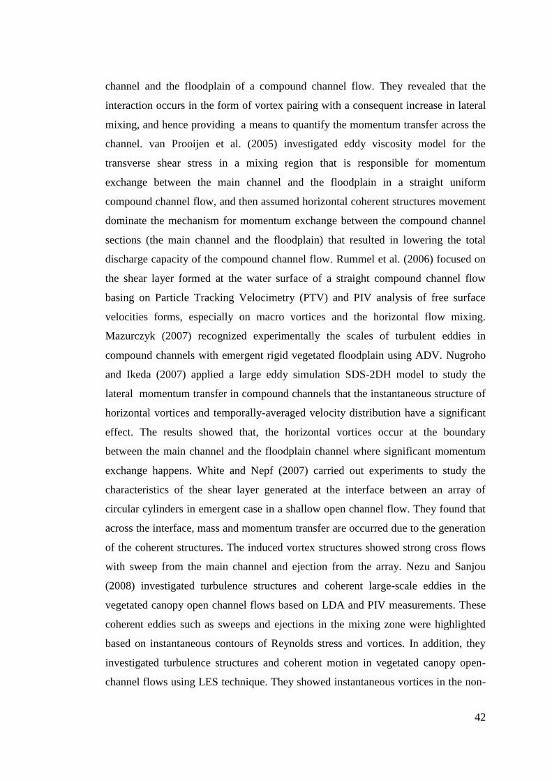
vegetated floodplain are adopted in this research as shown in Fig. 3.1. These setups
are one-line vegetation along the edge of the floodplain adjacent to the main channel
and wholly vegetated floodplain, which are then compared with the non-vegetated
floodplain.
(a) (b)
Fig. 3.1: Mixing process models in compound channel flows of the vegetated
floodplain (a) one-line vegetation along the edge of the floodplain, and (b) wholly
vegetated floodplain with a staggered arrangement.
3.2 METHODOLOGY AND EXPERIMENTS SET UP
The experiments were carried out in the Hyder Hydraulics Laboratory at Cardiff
University, UK, using a 10 m long laboratory glass-walled flume of a recirculating
system, 1.2 m wide and 0.3 m deep. The flume slope was set up with 0.001 for all of
the experiments. A compound channel was designed with shallow flow conditions
by attaching plastic sheets along one side of the flume, with a width of 76 cm, a
thickness of 2.4 cm and channel side slope as 1(H):1(V). Holes were made along the
entire floodplain width with staggered arrangements with 𝑎𝑥 = 𝑎𝑦 = 12.5 cm.
Circular wooden rods were selected of diameters D = 1.25 cm, 2.5 cm and 5.0 cm,
attached to the bed of the floodplain in two configurations; first, wholly vegetated
floodplain with vegetation density defined by a solid volume fraction (SFV) as
sparse (D = 1.25 cm and SVF = 1.5%), medium (D = 2.5 cm and SVF = 6.2%) and
dense (D = 5.0 cm and SVF = 24.8%) as shown in Fig. 3.2; second, a one-line array
of vertically-oriented rod diameters placed along the edge of the floodplain adjacent
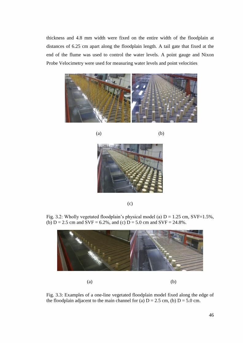
the main channel at 12.5 cm apart as shown in Fig. 3.3;. Transverse strips of 1.3 mm
46
thickness and 4.8 mm width were fixed on the entire width of the floodplain at
distances of 6.25 cm apart along the floodplain length. A tail gate that fixed at the
end of the flume was used to control the water levels. A point gauge and Nixon
Probe Velocimetry were used for measuring water levels and point velocities
(a) (b)
(c)
Fig. 3.2: Wholly vegetated floodplain’s physical model (a) D = 1.25 cm, SVF=1.5%,
(b) D = 2.5 cm and SVF = 6.2%, and (c) D = 5.0 cm and SVF = 24.8%.
(a) (b)
Fig. 3.3: Examples of a one-line vegetated floodplain model fixed along the edge of
the floodplain adjacent to the main channel for (a) D = 2.5 cm, (b) D = 5.0 cm.

47
Discharges were measured using the flow meter and calibrated by velocity
measurements and volume flow rate.
A thermal system was used that consists of a thermal camera of 30 Hz image
frequency and (640 X 480) pixel images resolution. This camera collects the infrared
radiation from objects in the scene and creates an electronic image based on
information about the temperature differences. The other parts of the thermal system
are water tank with heater and thermostat, injected tube and computer with FLIR
research IR software connects which is directly to FLIR thermal imaging cameras to
acquire thermal snapshots or movie files that can be stored on the SD-card. Two
moving rails across the compound channel section were used; at the first rail, a
thermal camera SC640 was mounted vertically above the water surface at a distance
of about 65 cm from the water surface of the flow for high resolution purposes and in
a section where the fully developed flow condition was achieved and a video capture
rate of five frames per second was applied. An arrangement was also achieved across
the rail to move the thermal camera laterally across the flume section by a slide
mean. On the second rail, the other parts of the thermal system were fixed, in which
the water tank connected to an injected tube, and the free end of the injection tube
was fixed at the water surface under a fully developed flow condition at 7.6 m from
the up-stream end of the flume working section. Figures (3.4 & 3.5) show a
schematic diagram of the thermal system arrangement that was used with the
compound channel flow section and a photograph of the system layout.
At the start, the flow runs under a uniform flow condition, hot water releases from
the water tank into the flume working section continuously via the injection tube
with a velocity equal to the velocity of the compound channel at the interface
between the main channel and the floodplain. As the thermal camera was fixed near
to the water surface, the area to be captured is in a part of the entire shear layer area,
which consists of 15 squares, five in the longitudinal direction and three squares in
the transverse direction, which were checked before the actual runs. Experiments
were achieved in such a way that the images have to be overlapped. To increase the
number of image sequences that are used in the analysis, two video files each of 187
sequences were recorded for each square.

48
The experiments were divided into three groups. Group one represents the case
without vegetation on the floodplain, with discharges of 4.66 l s-1
and 11.03 l s-1
. The
second group is considering a one-line of vegetation along the edge of the floodplain,
and three rod diameters were selected of D = 1.25 cm, 2.5 cm and 5.0 cm. With each
rod size two discharges (4.66 l s-1
and 11.03 l s-1
) were applied, as in the first group.
(a)
(b)
Fig. 3.4: A schematic diagram of system layout of the thermal camera across the
compound channel flow section.

49
Fig. 3.5: A photograph of the system layout showing the thermal camera, the
injection tube, the water tank, and a computer that were fixed at two rails across the
compound channel section flow of 1.2 m width in the presence of one-line vegetation
along the edge of the floodplain.
The third group is dealing with the wholly vegetated floodplain with the same rod
diameters as described in group two (D = 1.25 cm, 2.5 cm and 5.0 cm), and with
vegetation densities as a solid volume fraction, of sparse (SVF = 1.5%), medium
(SVF = 6.2%) and dense (SVF = 24.80%) respectively. Similarly, two discharges
were used as with the case studies of one-line vegetation and without vegetation on
the floodplain tests (Q = 4.66 l s-1
and 11.03 l s-1
).
The hydraulic characteristics of the experiments are explained in the Table 2.1. In
this table calculation of the Reynolds numbers is based on the bulk velocity, Ub and
the cylinder diameter, ReD = UbD/ν for the compound channel flows with vegetated
floodplain, and based on the bulk velocity , Ub and the water depth, H for the non-
vegetated floodplain cases. The Reynolds number range in the compound channel
flows is, ReD = 1700 - 12200. The Froude number calculations for uniform flow was
in the range of Fr = 0.16 - 0.26 which states subcritical flow, is based on the bulk
velocity, Ub as Fr = Ub/(gH) 0.5
, where H is the flow depth in the main channel, and g
is the gravitational acceleration.

50
Table 2.1: Hydraulic characteristics of flow conditions in compound channel section
with and without vegetated floodplain.
Case Discharge Water Bulk Reynolds Froude
study depth velocity number number
Q Hmc hf Ub ReD ReH Fr
(l/s) (cm) (cm) (cm/s)
Without 4.66 3.96 1.56 16.07 6327 0.26
vegetation 5.82 4.61 2.21 15.82 7249 0.24
7.51 5.26 2.86 16.84 8806 0.23
8.87 5.59 3.19 18.27 10152 0.25
11.03 6.12 3.72 20.08 12214 0.26
Wholly 4.66 4.46 2.06 13.32 6619 0.20
vegetated 5.82 5.14 2.74 13.48 6699 0.19
(Dense) 7.51 6.18 3.78 13.50 6709 0.17
D=5.0cm 8.87 6.99 4.59 13.57 6746 0.16
11.03 7.95 5.55 14.34 7128 0.16
Wholly 4.66 4.37 1.97 13.74 3415 0.21
vegetated 5.82 5.01 2.61 13.98 3475 0.20
(Medium) 7.51 6.20 3.80 13.44 3340 0.17
D=2.5cm 8.87 7.00 4.60 13.55 3367 0.16
11.03 7.95 5.55 14.34 3564 0.16
Wholly 4.66 4.35 1.94 13.87 1724 0.21
vegetated 5.82 4.89 2.49 14.48 1800 0.21
(Sparse) 7.51 6.05 3.65 13.89 1726 0.18
D=1.25cm 8.87 6.69 4.29 14.36 1785 0.18
11.03 7.78 5.38 14.73 1831 0.17
One-line 4.66 4.39 1.99 13.64 6782 0.21
vegetation 5.82 5.12 2.72 13.55 6736 0.19
D=5.0cm 7.51 5.83 3.43 14.60 7257 0.19
8.87 6.49 4.09 14.94 7428 0.19
11.03 6.98 4.58 16.90 8400 0.20
One-line 4.66 4.22 1.82 14.51 3606 0.23
vegetation 5.82 4.71 2.31 15.31 3804 0.23
D=2.5cm 7.51 5.39 2.99 16.27 4044 0.22
8.87 5.95 3.55 16.78 4169 0.22
11.03 6.54 4.14 18.39 4570 0.23
One-line 4.66 4.22 1.82 14.51 1803 0.23
vegetation 5.82 4.69 2.29 15.41 1914 0.23
D=1.25cm 7.51 5.34 2.94 16.49 2049 0.23
8.87 5.78 3.38 17.45 2168 0.23
11.03 6.14 3.74 19.99 2484 0.26

51
3.3 RESULTS AND DISCUSSIONS
3.3.1 Image Processing Technique
At the end of recording video files, the next step is to export these sequences from
the thermal camera into the FLIR software first, and then transferred them from the
FLIR software to Matlab files. The information that transmitted in Matlab files is not
directly temperatures. The information was in another sort of scale which is called a
colour code that should be converted into temperature values. When getting the
images with FLIR, the user has to set up the maximum and minimum range for the
temperature. In the Matlab files, it is specified the maximum and minimum values
for the colour code for getting out the relationship between the colour code values
and temperature values. Knowing this fact, enables transformation the Matlab values
into Celsius values. The average temperature calculation from a series of sequences
of 187 images (640 X 480 pixels) was carried out for each part of the shear layer
area. Since the recorded sequences were carried out for each part of the entire shear
layer twice, an average temperature of each two recording videos was achieved for
the entire shear layer parts. Then, a longitudinal overlapping for the entire shear
layer parts at the centre, left and right is required.
Overlapping between the successive squares was done first for the centre part as
follows; between the first and the second images to get a new image. Then the new
image overlaps with the third image and so on till the fifth image. Any overlap
between any two successive images had to go through a trial and error process with
high accuracy in order to select the most suitable overlap. In a similar way the
longitudinal overlapping was achieved to the left and right parts. At the end, three
parts (centre, left and right) were being prepared for the second step. A horizontal
overlapping may be needed between the centre and the left and the centre and the
right parts. An example of introducing a shear layer form in a compound channel
flow at the interface between the main channel and the floodplain was presented with
wholly vegetated floodplain of sparse density. The results showed the mean (187x2)
raw shear layer images of wholly vegetated floodplain as explained in Fig. 3.6.

52
(a) (b)
(c) (d)
(e)
Fig. 3.6: Raw images at five longitudinal locations for a wholly vegetated floodplain
with rod diameter, D = 1.25 cm, SVF = 1.5% and flow rate, Q = 4.66 l s-1
. (a) Raw
image of the first square (b) Raw image of the second square (c) Raw image of the
third square (d) Raw image of the forth square (e) Raw image of the fifth square.
(All the dimensions in pixels).

53
Figure 3.7 shows the steps of the longitudinal overlapping at the centre location
between the first and the second squares represents overlap 1, and then between the
results of the first overlap with the third square and so on up to the end of the
squares. The other five locations on either side of the centre part were similarly
carried out with longitudinal overlaps to create the second and the third parts for the
entire shear layer as left and right parts (see Fig. 3.8).
(a) (b)
(c) (d) (e)
Fig. 3.7: Image processing in the longitudinal direction of the centre part at five
squares for the case study of wholly vegetated floodplain with rod diameter, D =
1.25 cm, SVF = 1.5% and flow rate Q = 4.66 l s-1
. (a) Raw images of the first and the
second squares (b) Overlap 1 between the first and the second raw images (c)
Overlap 2 between the result of overlap 1 and the third raw image (d) Overlap 3
between the result of overlap 2 and the fourth image (e) Overlap 4 between the result
of overlap 3 and the fourth image. (All the dimensions in pixels).

54
(a) (b)
Fig. 3.8: Left and right parts of the shear layer resulted from the image processing
technique in the longitudinal direction for the five squares for the case study of
wholly vegetated floodplain with rod diameter, D = 1.25 cm, SVF = 1.5% and flow
rate, Q = 4.66 l s-1
. (a) Left side part of the shear layer on the floodplain shows the
rod diameters within the flow (b) Right side part of the shear layer on the main
channel. (All the dimensions in pixels).
To extract the final shear layer from the obtained three shear layer parts, a horizontal
overlapping was done for the left and the centre part of the shear layer first, and then
between the right part and the result of the overlap between the centre and the left
parts. The final results from Matlab of shear layer images were then exported into
Tec plot software as shown in Fig. 3.9.
In a similar way the longitudinal and the lateral overlaps were done for the other case
studies. The aforementioned description of image processing techniques using
Matlab and FLIR softwares was submitted as a conference paper (Mulahasan et al.
2015).

55
Fig. 3.9: Shear layer form at the interface between the main channel and the
floodplain for a wholly vegetated floodplain case of sparse vegetation density with
rod diameter of 1.25 cm and flow rate of 4.66 l s-1
. (All the dimensions in pixels).
3.3.2 Images of the Shear Layers
Two selected examples of time-averaged thermal images of 187 sequences are
shown in Fig. 3.10 as a part of the whole shear layer in the longitudinal direction of
the mixing shear layer that is generated at the interface between the main channel
and the floodplain in a compound channel flow. These are a wholly vegetated
floodplain with D = 5.0 cm and Q = 4.66 l s-1
, and with a one-line vegetation along
the edge of the floodplain with D = 2.5 cm and Q = 4.66 l s-1
. The x and y axis of the
drawings in Fig. 3.10 are normalized to water depth on the floodplain.
(a) (b)
Fig. 3.10: Examples of time-averaged thermal images normalized with flow depth on
the floodplain for the case of (a) Wholly vegetated floodplain with D = 5.0 cm and Q
= 4.66 l s-1
and (b) One-line vegetation with D = 2.5 cm and Q = 4.66 l s-1
.

56
To explain the evolution of the thermal distributions at different time intervals,
snapshots with intervals of 1/5 second were selected for the wholly vegetated
floodplain with rod diameter, D = 5.0 cm and flow rate, Q = 11.03 l s-1
as shown in
Fig. 3.11 which describes the penetration of the temperature inside the vegetated
floodplain.
(a) Snapshot after 1/5 second (b) Snapshot after 2/5 seconds
(c) Snapshot after 3/5 seconds
Fig. 3.11: Snapshots of the thermal images at time intervals of 1/5 second in the case
of the wholly vegetated floodplain with rod diameter D = 5.0 cm and Q = 11.03 l s-1
which is showing the impact (relative to shading factor due to drag by vegetation
causing lateral distribution) of the shear layer inside the vegetation elements and how
the temperature dissipates within the rods arrangements due to stream-wise velocity
and shear layer generated.
3.3.3 Effects of Vegetation
To visualize and evaluate the shear layer evolution at the interface between the main
channel and the floodplain, fourteen examples are considered to review the results of

57
two setups one-line vegetation and wholly vegetated floodplain compared to without
vegetation case. The final images of the shear layers are shown in Figs. (3.12-3.17);
these figures represent time-averaged temperature distribution. The mixing length
and the mixing width of the shear layers were normalized with water depth on the
floodplain. The analysis showed that the structure of turbulent mixing shear layers
(vortices) for a shallow water depth is very well captured and quantified by this
novel approach as described by the physical model in Fig. 3.1.
The impact of transverse flow depth variation and bed roughnessess are considered.
The impact of the roughness results in asymmetric shear layer about the vegetation
interface and the eddy structures are deformed due to mass and momentum transfer
between the main channel and the floodplain in the compound channel flows. The
shear layer evolution at the interface between the main channel and the floodplain
can be discussed as follows:
In the case of non-vegetated floodplain a symmetric leaf-shaped shear layer was
observed in the case of Q = 11.03 l s-1
. That is to say the penetration thickness inside
the vegetation δ1 equal to the penetration thickness inside the main channel δ2 as
shown in Fig. 3.15. However, the shear layer distribution at the interface between the
main channel and the floodplain is asymmetric for the case of Q=4.66 l s-1
due to the
impact of the flow depth variation between the main channel and the floodplain that
influencing the velocity gradient as shown in Fig. 3.12.
Figures of the shear layers manifest the evolution of the temperature distribution in
the x-y plane. The longest shear layer was monitored and observed in the non-
vegetated floodplain case studies in comparison with the cases of vegetated
floodplain. This can be imputed to absence of vegetation elements on the floodplain
that results in a less drag force. This is also can be seen in the time averaged
temperature distribution diagrams in Figs. 3.18 & 3.21.
In the one-line vegetation case, a similar trend to the non-vegetated floodplain was
observed with much more deformation to the shear layer shape, and the shear layer
length is shorter than that in the non-vegetated floodplain case due to the drag by the
one-line vegetation along the edge of the floodplain-main channel interface as shown

58
in Figs. 3.13 and 3.16 for the rod diameters (D =1.25, 2.5, and 5.0 cm) and flow rates
Q = 4.66 l s-1
and Q = 11.03 l s-1
respectively. The shear layer shape is significantly
influenced by the vegetation elements due to the increasing the velocity gradients
between the main channel and the floodplain in the compound channel flow, the
presence of dip velocity at the junction and due to the wake by the successive rods.
The velocity gradient reflects the momentum transfer between the vegetated and
non-vegetated sections. The length of the shear layer is decreased as the rod diameter
is increased or in increasing floodplain’s blockage factor (D/W), where D = cylinder
diameter and W = flume width. The rod diameter, D = 5.0 cm shows a significant
decrease in the shear layer length in comparison to the other two diameters (D =
1.25, and 2.5 cm), and the temperature distribution has a different propagation .The
(thermal) shear layer distribution for the smallest two diameters (D =1.25, and 2.5
cm) at the interface between the main channel and the floodplain shows the same
trend as with non-vegetated floodplain cases.
It was observed that the temperature distributions inside the main channel much
more than inside the floodplain and can be expressed by (δ1/δ2) < 1. This scenario
can also be seen in Figs. (3.19 & 3.22) in time averaged water temperature
distributions for Q = 4.66 l s-1
and Q = 11.03 l s-1
respectively.
The results of the shear layer distribution with the wholly vegetated floodplain case
studies are shown in Figs. (3.14 & 3.17) for sparse, medium and dense vegetation
densities, with Q = 4.66 l s-1
and Q = 11.03 l s-1
respectively. The mixing shear
layers have shown more penetration insde the main channel than that on the
floodplain as with one-line vegetation case studies and (δ1/δ2) < 1. This is because
the drag increases on the floodplain with increasing the vegetation density or with
high blockage and due to the wake of neighbouring cylinders. Figs. 3.14 (a, b and c)
show a significant impact of vegetation density on the shear layer length with Q =
4.66 l s-1
. Increasing the vegetation density on the floodplain results in a higher the
velocity gradient between the main channel and the floodplain; decreases the shear
layer length and increases the temperature distribution inside the vegetation elements
than that with one-line vegetation. Mass and momentum transfer between the
vegetated and non-vegetated sections due to the velocity differences. At high flow

59
rate (Q = 11.03 l s-1
), the impact of vegetation density on the shear layer length
shows almost the same explanations as with low discharge (Q = 4.66 l s-1
) as shown
in Fig. 3.17.
The shear layer shape for the wholly vegetated floodplain case studies has a less
deformed than that in one-line vegetation case studies. This scenario can be also seen
in Figs. (3.20 & 3.23) in time-averaged water temperature distributions with Q =
4.66 l s-1
and Q = 11.03 l s-1
respectively.
Fig. 3.12: Shear layer evolution at the interface between the main channel and the
floodplain in a compound channel flow for the case of non-vegetated floodplain with
Q = 4.66 l s-1
.
(a)

60
(b)
(c)
Fig. 3.13: Shear layer evolution at the interface between the main channel and the
floodplain in a compound channel flow in presence of one-line vegetation along the
edge of the floodplain adjacent to the main channel with Q = 4.66 l s-1
and rod
diameter of (a) D = 1.25 cm (b) D = 2.5 cm, and (c) D = 5.0 cm.

61
(a)
(b)
(c)

62
Fig. 3.14: Shear layer evolution at the interface between the main channel and the
floodplain in a compound channel flow for the case of the wholly vegetated
floodplain with Q = 4.66 l s-1
for vegetation density as (a) sparse (b) medium (c)
dense.
Fig. 3.15: Shear layer evolution at the interface between the main channel and the
floodplain in a compound channel flow for the case of non-vegetated floodplain for
Q = 11.03 l s-1
.
(a)

63
(b)
(c)
Fig. 3.16: Shear layer evolution at the interface between the main channel and the
floodplain in a compound channel flow in presence of one-line vegetation along the
edge of the floodplain adjacent to the main channel with Q = 11.03 l s-1
for rod
diameter of (a) D = 1.25 cm (b) D = 2.5 cm, and (c) D = 5.0 cm.

64
(a)
(b)
(c)

65
Fig. 3.17: Shear layer evolution at the interface between the main channel and the
floodplain in a compound channel flow for the case of the wholly vegetated
floodplain with Q = 11.03 l s-1
and vegetation density as (a) sparse (b) medium and
(c) dense.
3.3.4 Time-averaged temperature distribution
Time-averaged temperature distributions were extracted at four sections across the
shear layer evolution. These sections were normalized to water depth on the
floodplain, hf and represented by (0h, 2h, 4h and 10h). Results of time-averaged
temperature distributions reflect an index of penetration the shear layer within the
vegetation zone and inside the main channel, and shear layer evolution as shown in
Figs. (3.18-3.23).
Fig. 3.18 shows the time averaged-temperature distribution in the case of the non-
vegetated floodplain for flow rate of Q = 4.66 l s-1
. It has been shown that time
averaged-temperature distributions were conducted at sections downstream the
ambient of the injected hot water. After a small distance from the source of injecting
the hot water, steep variation in the temperature distribution was observed, for
example, the peak temperature (about 80 centigrade) sharp decreases in the direction
of the flow and its peak after a small distance was reduced to less than 40-60% of its
peak value at the point where the hot water was released. In addition, the lateral
distribution displays the peak value which is considered at the interface where the
point of injection hot water, while it continuously decreases laterally, in which after
a small distance the temperature reaches the temperature degree of the running water
in the flume. A significant decrease in the water temperature degree from a peak to a
value of 23 oC is due to the turbulent mixing between compound channel sections. In
a similar way, at high discharge case (Q = 11.03 l s-1
), the shear layer is showing the
same trend as for (Q = 4.66 l s-1
), but with less shear layer thickness as shown in
Figure (3.21). Mass and momentum transfer from the main channel (high velocity) to
the floodplain (low velocity).
The vegetated floodplain case studies (Figures 3.19, 3.20, 3.22 and 3.23) were
analysed. It has been shown that with the one-line vegetated floodplain (Figs. 3.19 &
3.22), the time averaged water temperature distributions depend on rod diameter,

66
blockage and flow rate considerations for Q = 4.66 l s-1
and Q = 11.03 l s-1
respectively. The temperature distribution in the longitudinal and transvers directions
was also explained in the shear layer evolution plots (see section 3.3.3).
Time averaged water temperature distributions with wholly vegetated floodplain
shows the evolution of the shear layers inside the vegetation and is affected by the
vegetation density as shown in Figs. 3.20 and 3.23 for Q = 4.66 l s-1
and Q = 11.03 l
s-1
respectively. The distribution of the (thermal) shear layer inside the vegetation
elements is increased with increasing vegetation density due to the velocity reduction
on the floodplain in comparison with one-line vegetation.
Fig. 3.18: Time-averaged water temperature distribution at the interface between the
main channel and the floodplain for a compound channel flow of non-vegetated
floodplain for Q = 4.66 l s-1
.

67
(a)
(b)

68
(c)
Fig. 3.19: Time-averaged water temperature distribution at the interface between the
main channel and the floodplain for a compound channel flow of one-line vegetation
along the edge of the floodplain with Q = 4.66 l s-1
and rod diameter of (a) D = 1.25
cm (b) D = 2.5 cm and (c) D = 5.0 cm.
(a)

69
(b)
(c)
Fig. 3.20: Time-averaged water temperature distribution at the interface between the
main channel and the floodplain for a compound channel flow of the wholly
vegetated floodplain with Q = 4.66 l s-1
for vegetation density as (a) sparse (b)
medium and (c) dense.

70
Fig. 3.21: Time-averaged water temperature distribution at the interface between the
main channel and the floodplain for a compound channel flow of non-vegetated
floodplain for Q = 11.03 l s-1
.
(a)

71
(b)
(c)
Fig. 3.22: Time-averaged water temperature distribution at the interface between the
main channel and the floodplain for a compound channel flow of one-line vegetation
along the edge of the floodplain with Q = 11.03 l s-1
and rod diameter of (a) D = 1.25
cm (b) D = 2.5 cm and (c) D = 5.0 cm.

72
(a)
(b)

73
(c)
Fig. 3.23: Time-averaged water temperature distribution at the interface between the
main channel and the floodplain for a compound channel flow of the wholly
vegetated floodplain with Q = 11.03 l s-1
for the vegetated density of (a) sparse (b)
medium and (c) dense.
3.3.5 Confirmation of the Models
For high image resolution, temperature values were extracted for each sequence at
five selection points in the wake region using Matlab software. The results showed
that the two kinds of vortices (shear layer vortices and von Karman vortices) that
were suggested in the model in Fig. (3.1) may be produced and good results can be
expected as shown in Figure (3.24).
(a) (b)

74
Fig. 3.24: Two kinds of coherent structures (shear layer vortices and von Karman
vortices) generated at the interface between the main channel and the floodplain with
(a) One-line vegetation, with D = 5.0 cm and Q = 11.03 l s-1
and (b) Wholly
vegetated floodplain, D = 2.5 cm and Q = 11.03 l s-1
.
3.3.6 Properties of the Vortices
To evaluate the development of eddies in the wake of the rods for the numbers of
runs that were carried out with thermal camera SC640, it was shown that vortical
structures are very clear in the densely vegetated floodplain (see Figure 3.25) as
shown in the most suitable areas for eddies and turbulences in the selected run
(wholly vegetated floodplain, D = 5.0 cm and Q = 4.66 l s-1
) after watching many
videos of the entire shear layer squares, where the rate of vortex rotating is very
high. This was done for five selection points in the wake area as shown in Figures
(3.24) for other vegetation cases. A clear wake behind the cylinder in the case of
medium vegetation case (D = 2.5 cm) is shown in Figure (3.24 b) and an area of high
velocities between the cylinders is observed, while in the case of dense vegetated
floodplain, flow field exhibits large velocity gradients in both stream-wise and span-
wise directions as shown in Figure (3.25), these were described in details in
(Stoesser et al. 2010) reference.
Shear layer vortices are usually occurring at the interface between vegetated and
non-vegetated zones as shown in Figure (3.24 a) for a one-line vegetation, while von
Karman vortices are formed behind the cylinder at short distance as a counter
rotating vortex pair for the case of D = 2.5 cm as shown in Figure (3.24 b), while for
dense vegetated floodplain D = 5.0 cm, the interaction of the stream-wise velocity
and span-wise velocity between rods inhibit these types of vortices. The time series
of temperature for the 187 sequences of the five selected points in the area of eddy
formation that locates between successive rods which were located in staggered
arrangements is shown in Figure (3.26). Successive peaks are shown in Figure (3.26)
along the time series frame (37 seconds) for all the five selected points in the wake
region relative to the stream-wise velocity and the rotation of the vortices. To extract
the energy of these eddies for the selected five points in the wake of the rods; Fourier
transforms are used and explained in Figure (3.27). This graph shows that the energy

75
of the eddies is small at high frequency, while for low frequencies there are large
eddies.
Fig. 3.25: Example of eddies formation in the wake of the rods for wholly vegetated
floodplain with D = 5.0 cm and flow rate of Q = 4.66 l s-1
which shows location of
five selection points.
Fig. 3.26: Time series for the five point selection in the wake of the rods for a period
of 37 seconds and the 187 sequences for wholly vegetated floodplain of D = 5.0 cm
and flow rate of Q = 4.66 l s-1
.

76
Fig. 3.27: Fourier transforms for the five selected points in the wake of the rods for
the case of the wholly vegetated floodplain of D = 5.0 cm and flow rate of Q = 4.66 l
s-1
.
3.4 CHAPTER SUMMARY
This chapter explains a novel approach to predicting and visualizing the evolution of
shear layer formation using thermal video sequences at the interface between the
main channel and the floodplain in a compound channel of shallow uniform flow.
Experiments were carried out in a laboratory flume of 10 m length and 1.2 m width
and for which uniform flow conditions were established for different flow rates. Hot
water was added at the water surface using a small tube at ambient condition and at
the interface between the main-channel and the floodplain where a fully developed
flow had been achieved. A thermal camera (SC640) operates at 5Hz frequency and
640X480 pixels resolution was mounted vertically at 0.65 m above a shallow flow
compound channel at the interface between the main channel and the floodplain at a
section where a fully developed flow had been achieved. This set-up enabled the
capturing of the flow temperature differences at 5 locations longitudinally and at 3
locations transversely.

77
Flir’s image processing software and Matlab were used to extract and analyse the
captured water surface temperature data. Image processing was done for the first to
fifth location at the junction edge of the floodplain adjacent to the main channel with
longitudinal overlaps to the images; between the first and the second image thus
creating the first overlap and then between the first image overlap and the third
image to create the second overlap and so on to the fifth image, thus creating the first
part of the shear layer at the centre. The other five locations on either side of the first
part that are located at the centre were similarly carried out with longitudinal
overlaps to create the second and the third parts of the shear layer as left and right
parts. At the end, three parts were acquired representing the entire shear layer. In
order to visualize the final shear layer (from these three parts), a horizontal overlap
was done for the left and the centre parts first, and then overlap between the right
and the results of the overlapping between the centre and left parts was achieved
secondly. The created shear layer image was then exported into Tecplot software.
The analysis showed that the shear layer at the interface between the main channel
and the floodplain is well captured and quantified by this technique.
Dynamics of shear layer evolution at the interface between the main channel and the
floodplain in compound channel flows with and without vegetation on its floodplain
was well quantified and evaluated by the thermal camera technique. The two setups
are shown in Figs. (3.24 a and b) which verified the aim of acquiring the shear layer
and von Karman street vortices. The shear layer elongation and propagation at the
interface between the main channel and the floodplain showed that the penetration of
the temperature inside the main channel is more than that on the floodplain for all the
vegetated floodplain cases and the distribution of the shear layer in the x-y plane is
influenced by the vegetation density, vegetation configuration and the flow rate. The
impact of the flow depth variation and roughness are explained in asymmetric shear
layer about the MC/FP interface. Time-averaged temperature distribution was well
described in all the case studies to appear as the shear layer evolution along the
streamwise direction and its propagation inside the floodplain and on the main
channel in the compound channel.

78
Eddies characteristics at the wake of the neighbouring rods are well described by
Fourier transforms graph as shown in Fig. (3.27). The results showed that the energy
of the eddies is small at high frequency, while for low frequencies they are large
eddies.

79
CHAPTER FOUR
FLOW RESISTANCE OF IN-LINE
VEGETATION IN OPEN CHANNEL
FLOW

80
4 FLOW RESISTANCE OF IN-LINE VEGETATION IN OPEN CHANNEL
FLOW
4.1 INTRODUCTION
Naturally-occurring vegetation in waterways is usually arranged in an irregular,
spatially heterogeneous fashion as a result of local variations in hydro-
geomorphology. In recent years several researchers have studied experimentally and
numerically the drag characteristics of arrays of submerged and emergent flexible
and non-flexible idealized vegetation arrays (Nepf 1999, Wu et al. 1999, Tsihrintzis
et al. 2001, Järvelä 2008, Stone and Shen 2002, Jarvela 2004, Jordanova et al. 2006,
James et al. 2008, Tanino and Nepf 2008, Kothyari et al. 2009, Stoesser et al. 2010,
Cheng and Nguyen 2011, Aberle and Järvelä 2013, Cheng 2013, Marjoribanks et al.
2014) or individual plants, e.g. (Yagci and Kabdasli 2008, Wunder et al. 2011).
However, under flood conditions when overbank flow produces a compound
channel, riparian vegetation such as trees and bushes may form one-line arrays of
emergent vegetation at the main channel-floodplain interface. This scenario is known
to make significant contributions to the overall hydraulic resistance of the channel
(Sun and Shiono 2009, Terrier et al. 2010). For instance, Terrier et al. carried out
compound channel experiments in a flume of length 8 m and width 1.2 m, with one
line of 9 mm diameter rods placed along the edge of the floodplain. They found that
the presence of the vegetation on the edge of the floodplain has a clear impact on the
stage-discharge curve compared to the case without vegetation. Detailed
measurements of the hydrodynamic behaviour of in-line vegetation are scarce.
Shiono et al. (2012) carried out flow measurements using an Acoustic Doppler
Velocimeter (ADV) in a single rectangular channel that was 9.0 m long and 91.5 cm
wide. Wooden rods of 9.0 mm diameter were fixed at the centre line of the channel
with a rod spacing 𝐿𝑠/D= 17.8 and a bed slope of 0.001. As would be expected,
slower velocities were observed near the rods.
Some common patterns of vegetation is growing at the edge of UK Rivers are
straight lines, such as the River Dove at Lovedale, the River Dove at Milldale, and
the River Severn at Ironbridge Gorge as shown in Figure 4.1.

81
Figure 4.1: Some common patterns of vegetation at the edge of UK Rivers are
straight lines, such as the River Dove at Lovedale, the River Dove at Milldale, and
the River Severn at Ironbridge Gorge.
In order to carry out accurate predictions of flood stages in natural waterways lined
with vegetation on its banks or floodplains accurate knowledge of the prevailing drag
coefficient (CD) is needed. Kim and Stoesser (2011) have demonstrated that
numerical models that are employed to predict flow resistance of emergent
vegetation rely heavily on accurate knowledge of the drag coefficient CD. Based on
laboratory and numerical data Tanino and Nepf (2008), Kothyari et al. (2009),
Cheng and Nguyen (2011) and Cheng (2013) propose simple empirical equations to
predict CD; these equations can be very useful for practitioners and numerical
modellers. However, they are based on experiments of arrays of vegetation and it is
unclear whether they are accurate in a one-line (or in-line) vegetation scenario.
The main aim of this research is to assess the suitability of various empirical
formulations to predict the drag coefficient of in-line vegetation. Equations evaluated
are the ones proposed by comparing predicted drag coefficients against experimental
data obtained as part of this study.
4.2 FLOW RESISTANCE IN VEGETATED STREAMS
For steady uniform flow, flow resistance through rigid emergent cylinders can be
estimated by equating the driving (gravitational) force of the flow to the bed
resistance and form drag (Figure 4.2), as given by Petryk and Bosmajian (1975):
𝐹𝐺 = 𝐹𝑓 + 𝐹𝐷 (4.1)
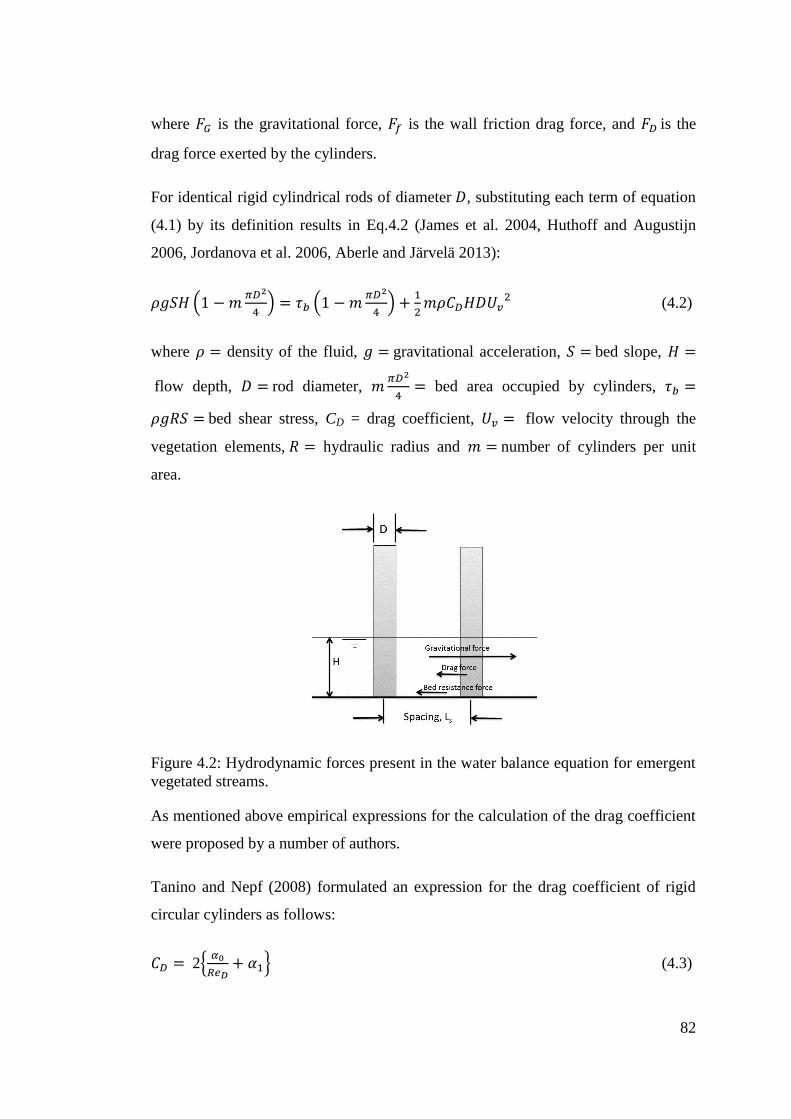
82
where 𝐹𝐺 is the gravitational force, 𝐹𝑓 is the wall friction drag force, and 𝐹𝐷 is the
drag force exerted by the cylinders.
For identical rigid cylindrical rods of diameter 𝐷, substituting each term of equation
(4.1) by its definition results in Eq.4.2 (James et al. 2004, Huthoff and Augustijn
2006, Jordanova et al. 2006, Aberle and Järvelä 2013):
𝜌𝑔𝑆𝐻 (1 − 𝑚𝜋𝐷2
4) = 𝜏𝑏 (1 − 𝑚
𝜋𝐷2
4) +
1
2𝑚𝜌𝐶𝐷𝐻𝐷𝑈𝑣
2 (4.2)
where 𝜌 = density of the fluid, 𝑔 = gravitational acceleration, 𝑆 = bed slope, 𝐻 =
flow depth, 𝐷 = rod diameter, 𝑚𝜋𝐷2
4= bed area occupied by cylinders, 𝜏𝑏 =
𝜌𝑔𝑅𝑆 = bed shear stress, CD = drag coefficient, 𝑈𝑣 = flow velocity through the
vegetation elements, 𝑅 = hydraulic radius and 𝑚 = number of cylinders per unit
area.
Figure 4.2: Hydrodynamic forces present in the water balance equation for emergent
vegetated streams.
As mentioned above empirical expressions for the calculation of the drag coefficient
were proposed by a number of authors.
Tanino and Nepf (2008) formulated an expression for the drag coefficient of rigid
circular cylinders as follows:
𝐶𝐷 = 2{𝛼0
𝑅𝑒𝐷+ 𝛼1} (4.3)

83
where 𝑅𝑒𝐷 is the cylinder or stem Reynolds number and 𝛼0 and 𝛼1 are functions of
the vegetation volume fraction (𝜙), which is the fraction of the overall volume that is
occupied by vegetation. 𝛼0 and 𝛼1 are empirical parameters which can be found in
Tanino and Nepf (2008).
Kothyari et al. (2009) proposed the following equation for the drag coefficient of
emergent cylindrical stems based on a set of fluid force measurements in subcritical
and supercritical flows:
𝐶𝐷 = 1.8𝜉𝑅𝑒𝐷−0.06[1 + 0.45 ln(1 + 100𝜙)] ∗ (0.8 + 0.2𝐹𝑟 − 0.15𝐹𝑟2) (4.4)
where, 𝜉 = parameter representing the cylinder staggered pattern, with 𝜉 = 0.8 for a
regular square staggered pattern and 𝜉 = 1.0 for the triangular-staggering stem
pattern, 𝜙 = 𝑚𝜋𝐷2/4 (area concentration of stems), and 𝐹𝑟 = 𝑈
√𝑔𝐻 (Froude
number), where 𝑈 is the bulk velocity, 𝐷 is the stem diameter, 𝑔 the acceleration due
to gravity and 𝐻 is the flow depth.
Cheng and Nguyen (2011) related the drag coefficient to the stem Reynolds number
using a new parameter, 𝑟𝑣, which represents the vegetation-related hydraulic radius
in a rectangular channel, which is defined as the ratio of the volume occupied by
water to wetted surface area of all cylinders as:
𝑟𝑣 =𝜋𝐷
4(
1−𝜙
𝜙) (4.5)
The drag coefficient is derived by considering the stream-wise force balance
equation for uniform flow and by neglecting frictional losses the drag coefficient is
calculated as:
𝐶𝐷 = 2𝑔𝑟𝑣𝑆
𝑈𝑣2 (4.6)
Cheng and Nguyen (2011) found that the dependence of CD on 𝑅𝑒𝐷 varies with
vegetation density and configuration (random or staggered). They showed that drag
coefficient decreases as Reynolds numbers increases.

84
Cheng (2013) proposed an alternative expression for the drag coefficient CD acting
on a sparse cylinder array and which he called the pseudofluid model:
𝐶𝐷 = 𝜋
2
1
𝜙
𝑔𝐷𝑆
𝑈𝑣2 (4.7)
where 𝑈𝑣 is the average flow velocity through emergent vegetation elements.
The suitability of equations (4.3) to (4.7) for the calculation of CD of in-line
vegetation is assessed and for which experiments were carried out.
4.3 EXPERIMENTAL PROCEDURE
Experiments were performed in the hydraulics laboratory of the School of
Engineering at Cardiff University, UK, using a recirculating glass-walled flume of
10 m length and 0.3 m width. Two uniform flow cases were investigated using bed
slopes of 0.001 and 0.0005. One line of wooden rods was attached to the bottom of
the flume, along its entire centreline, and the longitudinal centre-to-centre spacing of
the rods was 12.5 cm. Three different rod diameters were tested: D = 5.0 cm, 2.5 cm
and 1.25 cm, producing three corresponding spacing ratios of 𝐿𝑠 𝐷⁄ = 2.5, 5 and 10
respectively. The experimental setup is illustrated in Figure 4.3.
(a) (b)
Figure 4.3: Schematic diagram and photograph illustrating the experimental set-up
with one-line rod array in place.

85
Table 4.1 Hydraulic characteristics of open channel flow in the presence of one-line
vegetation at the centre line of the flume width.
Case Vegetation Bed Water Bulk Shear stress Froude Reynolds Reynolds
diameter Ls/D slope depth velocity ρgRS number number number
D (cm) % H (cm) Ub (cm/s) τ (N/m2)x10-2 Fr=Ub/(gH)0.5 ReD=UbD/ν ReH=UbH/ν
1 Lateral 0.05 3.8 17.63 14.8 0.29 - 6624
strips 0.05 5.2 19.16 19.0 0.27 - 9936
0.05 6.1 22.03 21.1 0.29 - 13249
0.05 7.1 23.40 23.7 0.28 - 16561
0.05 8.3 24.06 26.2 0.27 - 19875
0.05 8.9 26.24 27.4 0.28 - 23188
0.05 9.6 27.69 28.8 0.28 - 26506
0.05 10.3 29.04 30.0 0.29 - 29819
0.05 10.7 31.18 30.6 0.30 - 33133
2 D=1.25 10 0.05 4.9 13.68 18.0 0.20 1700 -
0.05 6.1 13.77 21.1 0.18 1711 -
0.05 6.9 14.40 23.3 0.17 1789 -
0.05 7.6 15.37 24.7 0.18 1910 -
0.05 8.5 15.68 26.6 0.17 1948 -
0.05 10.1 16.56 29.5 0.17 2058 -
3 D=2.5 5 0.05 5.6 10.47 19.9 0.14 2602 -
0.05 6.2 10.72 21.6 0.14 2662 -
0.05 7.5 11.05 24.6 0.13 2746 -
0.05 9.0 11.17 27.5 0.12 2776 -
4 D=5.0 2.5 0.05 6.9 7.27 23.1 0.09 3613 -
0.05 7.6 7.67 24.7 0.09 3812 -
0.05 8.3 8.01 26.2 0.09 3981 -
0.05 9.0 8.31 27.6 0.09 4130 -
0.05 9.7 8.58 28.9 0.09 4264 -
0.05 10.3 8.94 29.9 0.09 4443 -
5 Lateral 0.1 3.0 22.01 24.7 0.40 - 6607
strips 0.1 3.6 27.70 28.5 0.47 - 9940
0.1 4.4 30.59 33.1 0.47 - 13227
0.1 5.0 33.23 36.8 0.47 - 16549
0.1 5.5 36.54 39.3 0.50 - 19868
0.1 6.2 37.91 42.8 0.49 - 23176
0.1 6.6 40.62 44.8 0.51 - 26488
0.1 7.2 41.62 47.7 0.50 - 29788
0.1 7.6 43.85 49.5 0.51 - 33127
6 D=1.25 10 0.1 3.8 17.37 29.9 0.28 2158 -
0.1 5.3 19.01 38.2 0.26 2362 -
0.1 6.7 19.90 45.4 0.25 2473 -
0.1 8.0 20.84 51.1 0.24 2589 -
0.1 9.0 22.28 55.1 0.24 2768 -
0.1 10.0 23.40 58.8 0.24 2908 -
0.1 11.4 23.47 63.4 0.22 2916 -
7 D=2.5 5 0.1 4.0 13.62 31.0 0.22 3385 -
0.1 4.5 14.84 33.9 0.22 3688 -
0.1 5.4 15.46 38.9 0.21 3842 -
0.1 6.2 16.14 43.0 0.21 4011 -
0.1 7.0 16.70 46.7 0.20 4150 -
0.1 7.7 17.28 50.0 0.20 4294 -
8 D=5.0 2.5 0.1 5.3 10.34 38.3 0.14 5139 -
0.1 6.4 10.43 44.0 0.13 5184 -
0.1 7.7 10.77 50.0 0.12 5353 -
0.1 9.0 11.11 55.2 0.12 5522 -

86
To ensure uniform flow conditions, the flow depths were controlled by a tailgate that
was located at the downstream end of the flume’s working section. Water depths
were measured using point gauges located at 1 m intervals along the approach flow
section, upstream of the rods, to ensure no effects of incoming turbulence and
backwater impact. Depending on vegetation diameter, four to six flow rates were
tested for each rod diameter to investigate the rating curves, while nine flow rates
were used for the non-vegetated flume section with lateral strips. In all tests the stem
Reynolds numbers (𝑅𝑒𝐷 =𝑈𝑏𝐷
𝜈), were in the range 1700 < 𝑅𝑒𝐷 < 5500, and Froude
numbers, 𝐹𝑟 = 𝑈𝑏/√gH ranged from 0.09 to 0.51 (details of all experiments are
provided in Table 4.1). Uniform flow conditions were achieved for each experiment.
4.4 RESULTS
4.4.1 Water Level-Discharge Relationship
Figures 4.4 (a) and (b) present the water depth-discharge relationship with and
without one-line vegetation, for bed slopes of 0.0005 (a) and 0.001 (b) respectively.
The figures reveal that the introduction of one-line vegetation has a significant
impact on the water depth for a given discharge, i.e. for a given discharge, the water
depth increases as vegetation density, 𝜙, is increased. For very low discharges, the
curves are close to each other, but the curves diverge as discharge increases. For the
large-diameter rods the water depth rose very quickly above the length of the rods,
which only allowed maximum discharges of approximately 3 l/s.

87
(a)
(b)
Figure 4.4: Water depth-discharge relationships: a) bed slope 0.0005; b) bed slope
0.001.

88
4.4.2 Drag-Coefficient-Stem Reynolds Number Relationship
For steady uniform flow conditions, the flow resistance in a vegetated channel with
one–line rigid emergent cylinders can be estimated from equation (4.2). The drag
coefficient for a range of stem Reynolds numbers (𝑅𝑒𝐷 = 1700-5500) was calculated
with a mean value of 𝐶𝐷 ≅ 0.65. The flume was relatively narrow so that the
calculated 𝐶𝐷 values were corrected for flow blockage as proposed by Shields Jr and
Gippel (1995):
𝐶′𝐷 =𝐶𝐷
(1−𝐹𝐵)2 (4.8)
where 𝐹𝐵 is the blockage factor, which is defined as the ratio between the cylinder
diameter, 𝐷, to the flume width, 𝑊.
Figure 4.5 plots the drag coefficient as a function of stem Reynolds number using the
empirical equations proposed by Tanino and Nepf (2008), Kothyari et al. (2009),
Cheng and Nguyen (2011) and Cheng (2013) and the ones obtained from the
measurements of the present study for the 0.1% slope. The drag coefficient varies
between 𝐶𝐷 0.6 and 𝐶𝐷 1.0 and does appear to be somewhat sensitive to the stem
Reynolds number. Employment of Tanino and Nepf’s and Kothyari et al.’s equation
slightly overpredict the measured drag coefficients irrespective of 𝑅𝑒𝐷, however the
general trend that CD increases with increasing 𝑅𝑒𝐷 is predicted rather well by these
two equations. Cheng’s pseudo-fluid model and Cheng and Nguyen’s equations
obviously overpredict the viscous effect: their equations yields too large values at
lower stem Reynolds number, on the other hand the match between measured and
predicted CD is remarkably good at higher stem Reynolds number flows.

89
Figure 4.5: Drag coefficients as a function of stem Reynolds number as obtained
from measurements of this study and as computed using expressions from various
researchers.
A more quantitative comparison of predicted and measured drag coefficients for in-
line vegetation is possible with Figure 4.6, which plots measured drag coefficients
vs. those obtained using the four equations introduced above for both channel slopes.
Tanino and Nepf’s and Kothyari’s equations (Figure 4.6a and b) predict fairly
similar values throughout the range of Reynolds numbers covered. Tanino and
Nepf’s expression results in a consistent overestimation, probably because the
expression is based on their own experiments in which the vegetation was randomly
arranged and covered the entire width of the flume, whereas the drag coefficients of
the present study might benefit from a “shading effect”, i.e. the downstream cylinder
is positioned in the wake of the upstream cylinder and hence does not experience the
full hydrodynamic load. Kothyari’s expression also results in a consistent
overestimation of the drag coefficient, however slightly closer to the measured CD
values at lower 𝑅𝑒𝐷 than the ones predicted by Tanino and Nepf’s expression.
Similarly, Kothyari’s expression may only be suitable for in-line vegetation if

90
“shading” is taken into account. Cheng’s and Cheng and Nguyen’s expressions
overestimate vegetation drag for small to medium stem diameters irrespective of
channel slope. On the other hand a fairly good match is obtained for large stem
diameters. What is apparent from the experimental data is that in-line vegetation is
not very sensitive to the stem Reynolds number, if at all, then CD increases with
increasing 𝑅𝑒𝐷, whereas Cheng’s and Cheng and Nguyen’s expressions suggest an
opposite trend.
a) Tanino and Nepf (2008) b) Kothyari et al. (2009)
c) Cheng and Nguyen (2011) d) Cheng (2013)
Figure 4.6: Comparison of drag coefficient (measured versus calculated) for different
models.

91
4.5 CHAPTER SUMMARY
Experiments have been performed to measure the stage–discharge behaviour of open
channel flow through one line of vertically-oriented circular rods which mimics in-
line vegetation. Two bed slopes have been used, along with a range of rod diameters
which yielded different spacings between cylinders. For a series of uniform flows the
drag coefficient was calculated based on the measured uniform flow depth and under
consideration of the bed friction. Then the most prominent equations for calculating
the drag coefficient, CD, of vegetation have been employed to predict CD for the
experiments of in-line vegetation. Tanino and Nepf’s and Kothyari’s equations
consistently overestimate the measured drag coefficients but match the overall trend
of an increase of CD with increasing stem Reynolds number. Cheng’s and Cheng
and Nguyen’s expressions overestimate vegetation drag for low to medium values of
ReD whilst a good match has been achieved for the higher stem Reynolds numbers.
On the other hand the latter two expressions do not reflect the trend that of an
increase of CD with increasing stem Reynolds number.

92
CHAPTER FIVE
HYDRODYNAMICS OF COMPOUND
CHANNELS WITH VEGETATED
FLOODPLAIN

93
5 HYDRODYNAMICS OF COMPOUND CHANNELS WITH
VEGETATED FLOODPLAIN
5.1 INTRODUCTION
The middle and lowland stretches of most rivers are characterised by compound
cross sections that comprise one or two floodplains and a deeper main channel.
Vegetation may be distributed across the floodplains in a variety of ways, including
patches of bushes, grassy meadows and regular arrays of trees that line the edges of
the main channel and follow its meanders. Such arrays may occur naturally or by
design as part of flood protection or habitat creation programs, and may exert
significant influence on the hydraulic properties of the compound channel during
flood events. One of the most prevalent arrangements is commonly known as “one-
line” vegetation which comprises a single line of trees along the side of the main
channel, but arrays of trees that extend much further across the floodplain may also
occur.
Although a number of studies have focused on turbulence, secondary currents and
momentum transfer in non-vegetated compound channels (Tominaga and Nezu
1991, van Prooijen et al. 2005, Yang et al. 2007, Vermaas et al. 2011), the influence
of floodplain vegetation on the flow conditions in compound channels is less well
understood. The impact of vegetation density, 𝜙 on the water depth-discharge curve
has been studied experimentally by a number of authors for different vegetation
configurations; Ismail and Shiono (2006), Sun and Shiono (2009) and Terrier (2010)
considered one-line vegetation, while Nehal et al. (2012) and Hamidifar and Omid
(2013) investigated a wholly-vegetated floodplain. Masterman and Thorne (1992)
established a theoretical method to estimate the effects of bank vegetation on the
channel flow capacity, and showed that it is possible to relate these effects to the
channel width-to-depth ratio; the authors showed that the effect of bank vegetation
on channel discharge capacity declines rapidly as the width-to-depth ratio increases.
Ben-sheng et al. (2002) carried out experiments on a compound channel with a
narrow floodplain and showed that the influence of vegetation on the floodplain flow
capacity in such cases is not significant. Ismail and Shiono (2006) performed

94
experiments in compound meandering channels with floodplains that were covered
with small rectangular blocks to simulate vegetation. The authors carried out tests
with fixed and mobile bed sediments to assess the influence of floodplain vegetation
on sediment transport. The results showed that the influence of vegetation density on
stage discharge curve was minimal for the fixed bed case, but some variation was
observed for the mobile bed case. Yang et al. (2007) performed experiments in a
compound channel that was either unvegetated or fully covered with model
structures that were intended to represent grass, shrubs and trees. The authors found
that for a non-vegetated channel the streamwise velocities always followed a
logarithmic distribution, whereas S-shape velocity profiles were observed when
vegetation was introduced on the floodplain. Hirschowitz and James (2009)
estimated the total channel discharge in the presence of emergent vegetation along
the banks of a river as the sum of the discharges of the vegetated and clear channel
zones calculated seperately.
A number of researchers have studied the impact of vegetation density on the drag
coefficient for flow past arrays of emergent rigid cylinders (Petryk and Bosmajian
1975, Nepf 1999, Tanino and Nepf 2008, Kothyari et al. 2009, Stoesser et al. 2010,
Cheng and Nguyen 2011, Tinoco and Cowen 2013). Nepf (1999) proposed a model
for drag, turbulence and diffusion within emergent vegetation and showed that the
bulk drag coefficient decreases as vegetation density increases for both random and
staggered arrays. Tanino and Nepf (2008) conducted experiments involving flow
through a random array of emergent, rigid cylinders, investigating the effect of
Reynolds number and vegetation density on the resistance properties. It was found
that the bulk resistance decreased with increasing Reynolds number and increased
with increasing solid volume fraction.
Nehal et al. (2012) performed experiments to investigate the resistance properties of
one specific type of aquatic plant, Acorus Calmus L, showing that increases in
vegetation density are accompanied by significant increases in the water depth; a
staggered arrangement of the plants was found to produce the largest decrease in
flow rate. Hamimed et al. (2013) also found that the relationship between flow depth
and discharge depends strongly on the vegetation density; higher density leads to

95
larger water depth except for very shallow flows, which are largely insensitive to
changes in vegetation density. Hin et al. 2008 performed in situ flow measurements
in vegetated equatorial streams in Malaysia, arriving at an expression for the
apparent friction factor for a natural compound channel in terms of easily measurable
hydraulic parameters. The floodplains of the streams were very densely vegetated,
and as a result the floodplain flow was very small except when the overbank flow
was very large. The researchers observed that the apparent shear was very high at the
interface between the main channel and floodplain. Järvelä (2002) studied the
hydraulic characteristics of natural willows and sedges to understand how type,
density and combination of vegetation affects the bulk resistance in a channel. It was
shown that the resistance is highly dependent on the flow depth, velocity, Reynolds
number and vegetal characteristics.
In the case of one-line vegetation, a number of researchers have chosen to focus on
the influnece of the spacing ratio 𝐿𝑠/𝐷, where 𝐿𝑠 is the centre-to-centre distance
between the trees and D is the trunk diameter. Terrier (2010), for example, carried
out experiments for two spacing ratios, 𝐿𝑠/𝐷 = 8 and 16. Circular cylinders and
brushes were employed to represent vegetation without and with foliage,
respectively. The results showed that flow rate increased as 𝐿𝑠/𝐷 increased (i.e.
vegetation density decreased), except when foliage was added. Sun and Shiono
(2009) investigated the flow characteristics in a straight compound channel, with and
without one-line vegetation. Two vegetation densities were applied, 𝐿𝑠/𝐷 = 3.8 and
13.3, and it was observed that spanwise distribution of streamwise velocity changed
markedly with the introduction of vegetation. The boundary shear stress was also
significantly lower with one-line vegetation than without, which lead the authors to
conclude that sediment transport and bed scour during flood events will be reduced
by the introduction of rigid vegetation along floodplain edges, although there will be
an associated increase in water levels. Sun and Shiono (2009) also reported that the
discharge was reduced by 20-26% for 𝐿𝑠/𝐷 = 13.3 and 21-36% for 𝐿𝑠/𝐷 = 3.8
compared to the unvegetated floodplain case. Sanjou et al. (2010) tested a spacing
ratio of 𝐿𝑠/𝐷 = 5 in a compound channel of width ratio 𝐵comp/𝐵𝑚𝑐 = 2.50, where
Bcomp is the overall width and Bmc is the main channel width. They reported reduced

96
main channel velocities and altered spanwise distribution of velocities with the
inclusion of the one-line vegetation compared to the unvegetated base case; with
one-line vegetation two inflection points were observed in the spanwise profiles near
the main channel-floodplain interface, while there was just one inflection point for
the unvegetated compound channel section. These results suggest that significantly
less momentum transfer occurs between the main channel and floodplain when one-
line vegetation is introduced. Shiono et al. (2012) carried-out experiments in a flume
of length 9 m and width 0.915 m, with one-line vegetation with 𝐿𝑠/𝐷 = 17.8 and bed
width ratio 𝐵comp/𝐵𝑚𝑐 = 2.0. The velocity distribution was characteristics by bulges in
at the shear layer region near the water surface. Azevedo et al. (2012) modelled one-
line vegetation using steel rods of diameter D = 1.0 cm placed at a distance 1.0 m
apart, i.e. 𝐿𝑠/𝐷 = 100. Laser Doppler Velocimetry (LDV) was used to measure
velocities in a flume of length 11.6 m and width 0.79 m with 𝐵comp/𝐵𝑚𝑐 = 3.85.
Secondary currents were observed and two types of vortical structures, “bottom
vortex” and “free surface vortex”, that were absent from the unvegetated case, were
identified. Inclined up-flows were also observed to have higher magnitudes than in
the unvegetated case. Time-averaged velocities at different vertical cross sections
were shown to be similar except in the area near to the free surface due to the
presence of secondary currents. In the centre of the main channel the velocity
profiles were similar with and without one-line vegetation.
The effects of flow interaction between vegetated and non-vegetated regions in
compound open channels result in a spanwise distribution of the depth-averaged
mean velocity that is of tangential hyperbolic shape (van Prooijen and Uijttewaal
2002, White and Nepf 2007). Physical, mathematical, and analytical models have
been studied by a number of authors with a view of achieving accurate
representations of the spanwise distribution of streamwise velocities (Shiono and
Knight 1991, Pasche and Rouvé 1985, Pope 2000, van Prooijen and Uijttewaal 2002,
van Prooijen et al. 2005, Rameshwaran and Shiono 2007, White and Nepf 2007, Liu
and Shen 2008 , White and Nepf 2008, Tang and Knight 2008, Chen et al. 2010,
Tang et al. 2010, Teymourei et al. 2013, Yang et al. 2013, Li et al. 2014).
Experimentally, Pasche and Rouvé (1985) confirmed that depth-averaged velocities

97
are affected by vegetation in compound channel flows and showed that the inclusion
of vegetation reduced longitudinal flow velocities. van Prooijen et al. (2005)
proposed mechanisms for the momentum exchange in a straight uniform compound
channel flow by considering the spanwise profile of streamwise velocity. White and
Nepf (2007) showed that the velocity profiles separate the channel into two sections
of uniform velocity; vegetated and open channel, and a transitional region between
them. The spanwise variation of streamwise velocity in this transitional region is
characterised by a hyperbolic tangent curve. Yang et al. (2007) showed that spanwise
distribution of velocity in vegetated compound channels followed an S-shaped curve
with three distinct flow regions. Hamidifar and Omid (2013) found that inclusion of
vegetation on floodplains led to a decrease in the depth-averaged velocity over the
floodplain and an increase in the main channel. In their study the depth-averaged
velocity in both the main channel and floodplain decreased as vegetation density
increased. Valyrakis et al. (2015) showed experimentally how increasing riverbank
vegetation density on decreases the streamwise velocity on the riverbank while
increasing it at the main channel.
In this study, the effects of vegetation density and distribution on the rating curve,
the drag coefficients and the stream-wise velocity distribution in an asymmetric
compound channel are investigated experimentally. This study is organised as
follows: The next sections outline the theoretical framework on which the analysis is
based; after which the experimental methodology and set-up are introduced; the
experimental results are then, presented and discussed; and then finally some
conclusions are drawn.
5.2 THEORETICAL CONSIDERATIONS
Flow resistance in vegetated streams is due to a combination of form drag and skin
friction. The vegetation-induced drag force is given as follows:
𝐹𝐷 =1
2𝜌𝐶𝐷𝐴𝑓𝑈𝑎
2 (5.1)
where 𝐹𝐷 is the drag force acting on an individual stem, CD is the drag coefficient, Af
is the frontal area of the stem, 𝜌 is the density of water and 𝑈𝑎 is the average velocity

98
approaching the stem, which Cheng and Nguyen (2011) propose can be well
approximated by the average pore velocity through the vegetated region, Uveg
= (𝑄⁄𝑊H)/(1 − 𝜙), where Q is the bulk flow rate, 𝑊 is the channel width, H is the
flow depth and 𝜙 is the vegetation volume fraction or vegetation density, defined as
the ratio of the volume occupied by vegetation, Vveg, to the total volume, Vtot. Note
also that Cheng and Nguyen (2011) suggest Uveg = Uα = 𝑈𝑏 for low vegetation
density, where Uveg is the flow through the vegetation and 𝑈𝑏 is the bulk flow
velocity.
Estimation of the drag coefficient induced by vegetation elements in streams under
steady, uniform flow conditions can be established by equating the gravity force, FG,
to the drag force exerted by the vegetation elements, FD, as follows:
𝐹𝐺 = 𝐹𝐷 (5.2)
where,
𝐹𝐺 = 𝜌𝑔(𝐴𝑙 )𝑆 (5.3)
where ρ is the fluid density, g is the gravitational acceleration, A is the channel cross-
sectional area, l is the channel reach, and S is the bed slope. Equations (5.1-5.3) can
be rearranged to give the following expression for the drag coefficient:
𝐶𝐷 =2𝑔𝑆
𝑈𝑎2𝑎
(5.4)
where a is the vegetation density per unit length of the reach (m-1
), and can be
expressed as 𝑎 = 𝑚𝐷 , where m is number of stems per unit area occupied by the
stems. 𝑎 and 𝜙 are related as 𝜙 =𝜋
4𝑎𝐷. Equation 5.4 shows that the drag will
decrease as a increases.
Tanino and Nepf (2008) formulated the drag coefficient for floodplain flow through
an array of rigid circular cylinders as:
𝐶𝐷 = {𝛼0
𝑅𝑒𝐷+ 𝛼1} (5.5)

99
where 𝛼0 and 𝛼1 are functions of the vegetation volume fraction, 𝛼1 = 0.46 + 3.8 𝜙,
𝛼0 = 5.0 + 313.17𝜙, and 𝑅𝑒𝐷 = 𝑈𝑣𝑒𝑔𝐷/𝜈 is the cylinder Reynolds number, where
𝜈 is the fluid kinematic viscosity and Uveg is defined by Petryk and Bosmajian (1975)
as:
𝑈𝑣𝑒𝑔 = √2𝑔𝑆
𝐶𝐷𝑚𝐷 (5.6)
Kothyari et al. (2009) proposed the following equation for the drag coefficient of
emergent cylindrical stems based on a set of fluid force measurements in subcritical
and supercritical flows:
𝐶𝐷 = 1.8𝜉𝑅𝑒𝐷−0.06[1 + 0.45 ln(1 + 100𝜙)] ∗ (0.8 + 0.2𝐹𝑟 − 0.15𝐹𝑟2) (5.7)
where, 𝜉 is a parameter representing the effect of the vegetation staggering pattern,
with 𝜉 = 0.8 for a regular square staggering pattern and 𝐹𝑟 = 𝑈𝑣𝑒𝑔
√𝑔𝐻 is the Froude
number. The authors found that the drag coefficient varied only slightly with
Reynolds number but was very sensitive to changes in vegetation density. It should
be noted that, owing to the shortness of the vegetated area, the flow was not fully
developed and the authors speculated that drag coefficients were therefore higher
than they would have been for fully developed flow.
Cheng and Nguyen (2011) related the drag coefficient to Reynolds number by a new
parameter, the vegetation-related hydraulic radius, rv, which is defined as the ratio of
the volume occupied by water to the wetted surface area of all cylinders:
𝑟𝑣 =𝜋𝐷
4(
1−𝜙
𝜙) (5.8)
The drag coefficient and vegetation Reynolds number can then be expressed as
follows:
𝐶𝐷 = 2𝑔𝑟𝑣𝑆 𝑈𝑣𝑒𝑔2⁄ (5.9)
𝑅𝑒𝑣 = 𝑈𝑣𝑒𝑔𝑟𝑣 𝜈⁄ (5.10)
The authors found that dependence of 𝐶𝐷 on 𝑅𝑒𝑣 varies with vegetation density and

100
configuration (random or staggered) as also observed by (Tanino and Nepf 2008,
Kothyari et al. 2009).
In compound channel flows an apparent shear stress, 𝜏𝑖𝑛𝑡, arises due to the high
velocity gradients that are experienced at the interfaces between neighbouring
regions of the cross-section. The shear stress force 𝐹𝜏 is considered as:
𝐹𝜏 = 𝜏𝑖𝑛𝑡𝐴𝑠ℎ𝑒𝑎𝑟 (5.11)
where, 𝐴𝑠ℎ𝑒𝑎𝑟 is the shear area, and 𝜏𝑖𝑛𝑡 is the apparent shear stress.
This apparent shear stress, 𝜏𝑖𝑛𝑡 was defined by Huthoff (2007) as follows:
𝜏𝑖𝑛𝑡 =1
2𝛹𝜌(𝑈2
𝑚𝑐 − 𝑈2𝑓𝑝) (5.12)
where, 𝜓 = a dimensionless interface coefficient, 𝛹 ≈ 0.020, 𝑈𝑚𝑐 = velocity of the
flow in the main channel, 𝑈𝑓𝑝 = velocity of flow above the floodplain.
For one-line vegetation, because there are two dips at the interface between the main
channel and the floodplain, the interfacial shear stress is expressed as follows:
𝜏𝑖𝑛𝑡 =1
2𝜓𝜌[(𝑈2
𝑚𝑐 − 𝑈2𝑑𝑖𝑝) + (𝑈2
𝑓𝑝 − 𝑈2𝑑𝑖𝑝)] (5.13)
where, 𝑈𝑑𝑖𝑝 = velocity of the flow near to the interface.
In addition to the Huthoff (2007)’s expression, a number of methods for quantifying
the apparent shear stress at the interface between the main channel and the floodplain
were reviewed in (Thornton et al. 2000). Two of these methods have been used in
the present study. The first of these was derived by Rajaratnam and Ahmadi (1981)
and is defined as follows:
𝜏𝑖𝑛𝑡 = 0.15 (𝐻𝑚𝑐
ℎ𝑓− 1)
2
(𝛾ℎ𝑓𝑆) (5.14)
where, 𝐻𝑚𝑐 = depth of flow in the main channel, ℎ𝑓 = depth of flow on the
floodplain, 𝛾 = specific weight of water and 𝑆 = friction slope.
The second approach relates the shear stress, percentage blockage due to
vegetation, 𝐹𝐵 , flow depth, and flow velocities as follows:

101
𝜏𝑖𝑛𝑡 = 0.1025𝜏𝑏 (𝑈𝑓𝑝
𝑈𝑚𝑐)
−3.4148
(ℎ𝑓
𝐻𝑚𝑐)
2(1 − 𝐹𝐵) (5.15)
With one-line vegetation, drag coefficient is calculated from the following
expression:
𝐹𝐷 = 𝐹𝐺 − 𝐹𝑆 + 𝐹𝜏 (5.16)
where 𝐹𝑆 is the bed shear stress force and can be written as:
𝐹𝑆 = 𝜌𝑔𝑅𝑆 (5.17)
where 𝑅 is the hydraulic radius.
5.3 EXPERIMENTAL METHODOLOGY AND SETUPS
Experiments were carried out in a 10 m × 1.2 m × 0.3 m glass-walled recirculating
flume in the Hyder Hydraulics Laboratory at Cardiff University, UK. The bed slope
was set to 0.001 for all test cases. A compound channel with one floodplain was
installed in the flume by attaching slabs of plastic, 76 cm wide and 2.4 cm thick,
alongside one of the side walls. The floodplain was therefore 76 cm wide, and the
bankfull depth of the main channel was 2.4 cm (Fig. 5.1). The floodplain bed slope
was equal to that of the main channel, i.e. Smc = Sfp = S = 0.001. Flow depths were
controlled by a tailgate that was located at the downstream end of the flume’s
working section. Discharges were measured using a flow meter and calibrated by
velocity measurements and volumetrically. A point gauge and Nixon Probe
Velocimeter were used to measure water levels and point velocities respectively.
Wooden rods of three different diameters (D = 5.0 cm, 2.5 cm and 1.25 cm) were
used as laboratory models for rigid emergent vegetation elements. Three canonical
configurations were tested: unvegetated channel, wholly-vegetated floodplain and
one-line vegetation. For the case of the wholly-vegetated floodplain the rods were
inserted into holes that were drilled into the plastic floodplain in a staggered fashion;
the centre-to-centre separation of the holes in streamwise and spanwise directions
was 12.5 cm (Fig. 5.1a). This arrangement produced solid volume fractions of 24.8%
(dense vegetation), 6.2% (medium) and 1.5% (sparse) for the three different rod

102
diameters. For the case of one-line vegetation the rods were inserted into holes that
were drilled along a line parrallel to the sides of the flume: the streamwise centre-to-
centre separation of the holes was 12.5 cm and the hole centres were 2.5 cm from the
edge of the main channel (Fig. 5.1b). This arrangement produced normalised
vegetation spacings of 𝐿𝑠 𝐷⁄ = 2.5, 5 and 10 for the three different rod diameters.
Five discharges were tested for all vegetation configurations and rod diameters: 4.66
l s-1
, 5.87 l s-1
, 7.51 l s-1
, 8.87 l s-1
and 11.03 l s-1
. Table 5.1 provides a summary of
flow conditions for all test cases.
For each discharge the water depth at the centre of the main channel was measured at
streamwise intervals of 1 m in the section 3 m ≤ x ≤ 9 m. Measurements of mean
streamwise velocity, U, were carried out in sections in which the flow was
considered to be fully developed: for the wholly-vegetated floodplain, velocities in
two sections were measured (x = 4.76 m, and 8.52 m), while for the one-line case
four sections were considered (x = 4.76 m, 7.76 m, 8.15 m and 8.52 m). In the main
channel velocities were measured at two depths, 0.2𝐻𝑚𝑐 and at 0.8𝐻𝑚𝑐, and the
average was taken (𝑈 = 𝑈0.2𝐻𝑚𝑐+𝑈0.8𝐻𝑚𝑐
2 ). The first spanwise measurement location
was 6.5 cm from the main channel side-wall, and further measurements were taken
at 5 cm spanwise intervals until a distance 7 cm from the edge of the floodplain; over
this last 7 cm measurements were taken at 1 cm spanwise intervals to improve the
resolution in this complex region. On the floodplain the velocity was measured at the
mid-depth, i.e. 𝑈 = 𝑈0.5ℎ𝑓, with two measurements between neighbouring rods in
the same row taken. For the one-line vegetation case the same procedure was
followed in the main channel as for the wholly-vegetated case but on the floodplain
the velocities were measured at 5 cm spanwise intervals from the rod centre to the
side wall. For the unvegetated channel case the same procedure was adopted for the
main channel as for the other two cases, while on the floodplain measurements were
taken 5 cm spanwise intervals between the edge of the main channel and the side
wall.

103
(a)
41.6 cm 76.0 cm
2.4 cm
hf
2.4cm Hmc
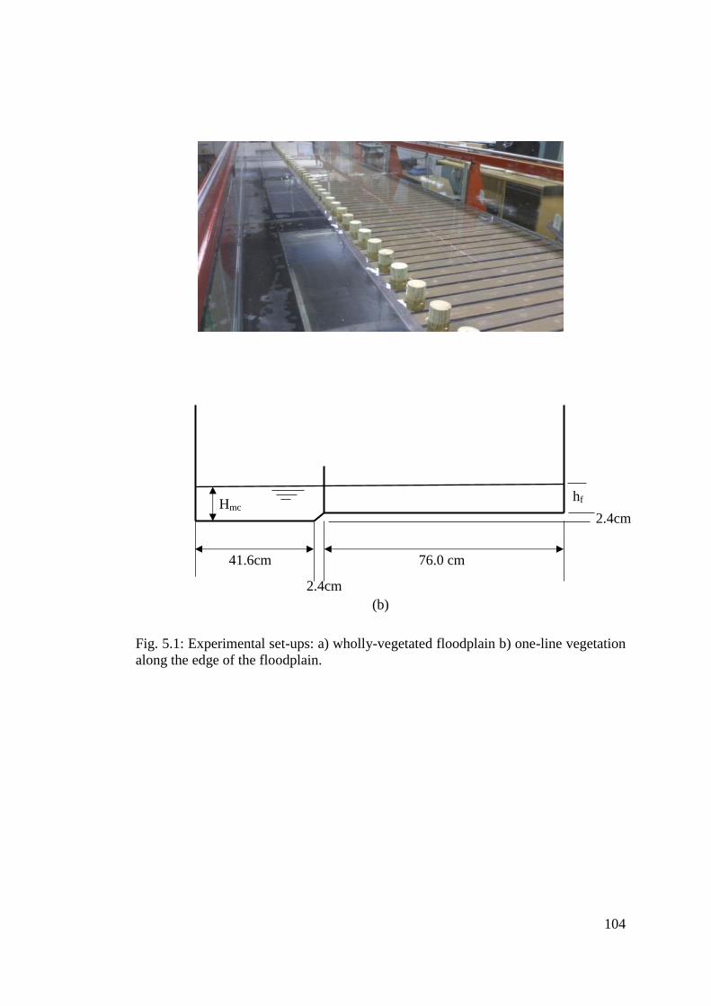
104
(b)
Fig. 5.1: Experimental set-ups: a) wholly-vegetated floodplain b) one-line vegetation
along the edge of the floodplain.
41.6cm 76.0 cm
2.4cm
hf
2.4cm Hmc

105
Table 5.1 Summary of flow conditions
Config. D
(cm)
Q
(l/s)
Hmc
(cm)
hf
(cm)
ubulk
(cm/s) ReD ReR Fr
SVF
(%)
Ls/D
Non-
vegetated
floodplain
-
4.66 3.96 1.56 16.07 - 3661 0.26
- 5.82 4.61 2.21 15.81 - 4523 0.24
- 7.51 5.26 2.86 16.84 - 5782 0.23
- 8.87 5.59 3.19 18.27 - 6794 0.25
- 11.03 6.12 3.72 20.08 - 8376 0.26
One-line
5.00 4.66 4.39 1.99 13.64 6781 3635 0.21 2.5
5.00 5.82 5.12 2.72 13.55 6736 4486 0.19 2.5
5.00 7.51 5.83 3.43 14.60 7257 5730 0.19 2.5
5.00 8.87 6.49 4.09 14.94 7427 6699 0.19 2.5
5.00 11.03 6.98 4.58 16.90 8400 8267 0.20 2.5
2.50 4.66 4.22 1.82 14.51 3606 3646 0.23 5.0
2.50 5.82 4.71 2.31 15.31 3804 4516 0.23 5.0
2.50 7.51 5.39 2.99 16.27 4044 5770 0.22 5.0
2.50 8.87 5.95 3.55 16.78 4169 6756 0.22 5.0
2.50 11.03 6.54 4.14 18.39 4570 8323 0.23 5.0
1.25 4.66 4.22 1.82 14.51 1803 3646 0.23 10
1.25 5.82 4.69 2.29 15.41 1914 4517 0.23 10
1.25 7.51 5.34 2.94 16.49 2049 5774 0.23 10
1.25 8.87 5.78 3.38 17.45 2168 6774 0.23 10
1.25 11.03 6.14 3.74 19.99 2484 8374 0.26 10
Wholly-
vegetated
5.00 4.66 4.46 2.06 13.32 6619 3633 0.20 24.8
5.00 5.82 5.14 2.74 13.48 6699 4486 0.19 24.8
5.00 7.51 6.18 3.78 13.50 6709 5700 0.17 24.8
5.00 8.87 6.99 4.59 13.57 6746 6650 0.16 24.8
5.00 11.03 7.95 5.55 14.34 7128 8148 0.16 24.8
2.50 4.66 4.37 1.97 13.74 3415 3638 0.21 6.2
2.50 5.82 5.01 2.61 13.98 3475 4495 0.20 6.2
2.50 7.51 6.20 3.8 13.44 3340 5699 0.17 6.2
2.50 8.87 7.00 4.6 13.55 3367 6649 0.16 6.2
2.50 11.03 7.95 5.55 14.34 3564 8148 0.16 6.2
1.25 4.66 4.35 1.94 13.87 1724 3639 0.21 1.5
1.25 5.82 4.89 2.49 14.48 1800 4503 0.21 1.5
1.25 7.51 6.05 3.65 13.89 1726 5712 0.18 1.5
1.25 8.87 6.69 4.29 14.36 1785 6681 0.18 1.5
1.25 11.03 7.78 5.38 14.73 1831 8169 0.17 1.5

106
5.4 RESULTS AND DISCUSSIONS
5.4.1 Impact of Vegetation on the Water Depth-Discharge Curve
The influence of vegetation density on the water depth-discharge relationship for the
wholly-vegetated floodplain case is shown in Fig. 5.2. The plot clearly illustrates that
in general the inclusion of a wholly-vegetated floodplain produces a marked increase
in water depth compared to the unvegetated case for a given flow rate. The increase
is smallest at the lowest flow rate and becomes more noticeable as flow rate
increases. As would be expected, increasing the rod diameter, and therefore the
vegetation density, results in further increases in water level. The water level
increases with flow rate in all cases: interestingly, water depth appears to increase
linearly with flow rate when the floodplain is vegetated but this is not the case for the
unvegetated channel. The mean increase in the water depth is 15.88%, 15.13% and
13.1% for dense, medium and sparse vegetation densities respectively.
Fig. 5.2: Stage-discharge curves for compound channel flow with wholly-vegetated
and unvegetated floodplains.
Figure 5.3 presents the variation of water depth with flow rate for the one-line
vegetation case. The inclusion of one-line vegetation produces a much smaller

107
increase in water depth compared to the wholly-vegetated floodplain (Fig. 5.2). This
is due to the fact that the overall vegetation density, and therefore flow blockage, for
the one-line case is naturally much smaller than in the full-vegetated case. The plot
does indicate, however, that water depth is noticeably more sensitive to changes in
𝐿𝑠 𝐷⁄ for one-line vegetation than to changes in density for a wholly-vegetated
floodplain. It can clearly be seen that there has been a significant increase in the
water depth as the vegetation density is increased in comparison with non-vegetated
floodplain (Fig. 5.2).
Fig. 5.3: Stage-discharge curves for compound channel flow with one-line vegetation
and unvegetated floodplain.
5.4.2 Estimation of mean drag coefficients
Fig. 5.4 presents the variation of drag coefficient with Reynolds number, based on
the bulk flow velocity and stem diameter, for the wholly-vegetated floodplain case.
The experimental drag coefficient values for the present study have been estimated
using the simple streamwise momentum balance, and are plotted alongside
experimental data from a number of previous experimental studies. In addition,
empirical relationships proposed by Tanino and Nepf (2008), Kothyari et al (2009)
and Cheng and Nguyen (2011) have been applied to the hydraulic conditions

108
investigated in the present study, and the resulting drag coefficient estimates have
also been included in the plot. Clearly the collated data shows that the drag
coefficient displays a high degree of sensitivity to changes in both Reynolds number
and vegetation density. The experimental data from the present study appears to
follow the general trend displayed by the other data sets, although there is
considerable scatter. It is interesting that the lowest density ratio data sets of Tinco
and Cowen (2013) (𝜙 = 1.0%) is the notable outlier from the general trend; in this
case the drag coefficient appears to be largely independent of Reynolds number.
Application of the empirical relationships to the hydraulic conditions tested in the
present study generally produces very close agreement with the measured drag
coefficients.
Fig. 5.4: Drag coefficient-Reynolds number relationship for wholly-vegetated
floodplain.
Fig. 5.5 shows the influence of rod diameter on the drag coefficient-Reynolds
number relationship for the case of one-line vegetation. The figure clearly shows that
drag coefficient decreases with increasing Reynolds number, and the range of

109
measured drag coefficient increases with decreasing rod diameter. As discussed in
the “Theoretical Considerations” section of this article, various researchers have
proposed different empirical relationships to allow the determination of the
interfacial shear stress in compound channels. Equations 5.12 to 5.15 have been used
to estimate the interfacial shear stress for the flow cases investigated in the present
study, and Fig. 5.6 reveals the effect of the choice of equation on the estimated drag
coefficient. Also included in the plot are data from the experimental study of Tanino
and Nepf (2008) and Tanino and Nepf (2008)’s proposed drag coefficient equation
for the wholly vegetated case. The plot reveals that the data from the present
investigation, which populate the Reynolds number range 1800 < Re < 8400, largely
follow the same trend as the experimental data of Tanino and Nepf. The plot also
suggests that the choice of empirical equation does not significantly affect the
estimation of drag coefficient: there is relatively little scatter between the four data
sets, with the exception of the lowest Reynolds number point when Equation 5.11 is
used.
Fig. 5.5: Impact of rod diameter on the drag coefficient-Reynolds number
relationship from water balance equation (FD = FG-FT-FS) for one-line vegetation.

110
Fig. 5.6: Drag coefficient-Reynolds number relationship: effect of choice of
theoretical approach to calculate interfacial shear stress.
5.4.3 Spanwise distribution of streamwise velocity
Figs 5.7 and 5.8 present spanwise profiles of mean depth-averaged streamwise
velocity for the wholly-vegetated floodplain and one-line vegetation cases
respectively. In each case the three sub-figures present data for the three different
flow rates that have been tested. Note that the velocity has been normalised on the
bulk streamwise velocity, ubulk. Profiles measured at two (Fig. 5.7) or four (Fig. 5.8)
streamwise locations are presented: the close agreement between profiles measured
at different streamwise locations indicates that the flow in the measurement section
of the flume was fully developed.

111
(a)
(b)

112
(c)
Fig. 5.7: Spanwise profiles of mean depth-averaged streamwise velocity for wholly-
vegetated floodplain with medium vegetation density (D = 2.5cm): a) Q = 4.66 l s-1
;
b) Q = 7.51 l s-1
; and c) Q = 11.03 l s-1
.
(a)

113
(b)
(c)
Fig. 5.8: Spanwise profiles of mean depth-averaged streamwise velocity for one-line
vegetation with rod diameter (D = 2.5cm): a) Q=4.66 l s-1
; b) Q = 7.51 l s-1
; and c) Q
= 11.03 l s-1
.

114
Fig. 5.9 presents comparisons of spanwise profiles of mean depth-averaged
streamwise velocity for the different configurations (unvegetated, wholly-vegetated
and one-line) for the three flow rates that were tested. Note that for the wholly-
vegetated floodplain and one-line cases only data pertaining to the D = 2.5cm cases
have been presented. Once again the velocity is normalised on ubulk. The plots
provide clear confirmation that, as would be expected, flow velocity above a wholly-
vegetated floodplain is noticeably lower than that above an unvegetated floodplain.
However the plots also reveal that the inclusion of one-line vegetation produces
higher velocities above the floodplain compared to the unvegetated case.
Correspondingly, the streamwise velocities in the main channel are highest for the
wholly-vegetated floodplain case, lowest for the unvegetated case and intermediate
for the one-line case. Also noteworthy are the characters of the velocity distributions:
for the wholly-vegetated and unvegetated floodplains the spanwise profiles follow an
S-shaped curve but for one-line vegetation the profiles exhibit a distinct dip at the
interface between the main channel and the floodplain.
(a)

115
(b)
(c)
Fig. 5.9: Spanwise profiles of mean depth-averaged streamwise velocity for wholly-
vegetated floodplain and one-line vegetation in comparison to non-vegetated
floodplain: a) Q = 4.66 l s-1
; b) Q = 7.51 l s-1
; and c) Q = 11.03 l s-1
.

116
Spanwise profiles of depth-averaged mean streamwise velocity for the case of an
unvegetated floodplain are shown in Fig. 5.10, illustrating the effect of flow rate on
the velocity distribution. The plot reveals that the normalised velocity in the main
channel decreases with increasing flow rate, while increasing above the floodplain.
Fig. 5.10: Spanwise profiles of mean depth-averaged streamwise velocity for
unvegetated compound channel.
Fig. 5.11 presents spanwise profiles of depth-averaged mean streamwise velocity for
the case of a wholly-vegetated floodplain. Each of the three sub-figures corresponds
to a different flow rate, and in each sub-figure data pertaining to the three vegetation
densities are plotted. In all cases the data exhibit S-shaped spanwise profiles, and the
velocity in the main channel increases with increasing vegetation density. The
floodplain velocities are shown to be largely independent of vegetation density, with
the exception of the highest flow rate case (Fig. 5.11c), where the floodplain velocity
is slightly larger for the lowest vegetation density.

117
(a)
(b)

118
(c)
Fig. 5.11: Impact of the vegetation density on the spanwise velocity profiles: a) Q =
4.66 l s-1
; b) Q = 7.51 l s-1
; and c) Q = 11.03 l s-1
.
Fig. 5.12 presents spanwise profiles of depth-averaged mean streamwise velocity for
the case of one-line vegetation, for the three different flow rates that have been
considered. The velocity gradients either side of the interface between the main
channel and the floodplain are very strong, leading to very high shear stresses and
strong large scale vortices. The profiles also reveal very pronounced local minima
close to the line of vegetation, indicating suppression of momentum transfer between
the main channel and the floodplain, which is in agreement with the findings of Sun
and Shiono (2009) and Shiono et al. (2012).

119
(a)
(b)

120
(c)
Fig. 5.12: Impact of one-line vegetation on the spanwise velocity profiles: a) Q =
4.66 l s-1
; b) Q = 7.51 l s-1
; and c) Q = 11.03 l s-1
.
5.5 CHAPTER SUMMARY
Laboratory experiments were carried out to quantify the influence of floodplain
vegetation on the rating curve, mean drag coefficient and spanwise distribution of
streamwise velocity in compound open channels. Two vegetation configurations -
wholly-vegetated floodplain and one-line vegetation - were tested along with a
smooth unvegetated compound channel. Vegetation elements were modelled by
emergent rigid wooden rods of circular cross-section. For the vegetated cases the
effect of vegetation density was investigated, and in all cases three flow rates were
tested.
The results showed that for a wholly-vegetated floodplain the water depth increased
by 15.88%, 15.13% and 13.1% for dense, medium and sparse vegetation densities,
respectively, compared to the unvegetated case. One-line vegetation produced a
smaller increase in flow depth than the wholly-vegetated floodplain. The results for
one-line vegetation showed that the water depth increased by 11.26%, 4.62% and

121
2.59% for vegetation diameters of 5.0cm, 2.5cm and 1.25cm, respectively, compared
to the unvegetated case.
It was observed that for a wholly-vegetated floodplain the drag coefficient increases
with increasing vegetation density. For all vegetation densities the drag coefficient
was observed to decrease as Reynolds number increased. Applying the empirical
equations of Tanino and Nepf (2008), Kothyari, et al. (2009) and Cheng and Nguyen
(2011) to estimate the drag coefficients for the hydraulic conditions presently tested
produced values in the range of experimental data from the literature, with relatively
little scatter. The experimentally-recorded drag coefficients agreed well with Tinco
and Cowen’s (2013) results for medium vegetation density, but the agreement for
low vegetation density is less convincing.
For one-line vegetation, it was observed that drag coefficient increases with
decreasing rod diameter. Empirical equations from the literature were used to
estimate the interfacial shear stress at the interface between the main channel and the
floodplain: accounting for the interfacial shear stress in this way produced more
accurate estimations of the overall drag coefficient compared to simply equating
drag force to the overall bed shear stress. Using Tanino and Nepf’s (2008) empirical
equation for the range of hydraulic parameters presently tested produced estimations
for drag coefficient in the region of 1.0.
Spanwise profiles of depth-averaged mean streamwise velocity confirmed that
introduction of a wholly-vegetated floodplain results in a considerable reduction in
floodplain velocities compared to the unvegetated case, while one-line vegetation
produces an increase in floodplain velocity. Velocity in the main channel is lower for
wholly-vegetated floodplains and higher for one-line vegetation. The spanwise
distributions of streamwise velocity for wholly-vegetated and unvegetated
floodplains follow S-shaped curves whereas for one-line vegetation a very
pronounced dip is observed at the interface between the main channel and the
floodplain.

122
CHAPTER SIX
FREE SURFACE FLOW OVER SQUARE
BARS AT LOW AND INTERMEDIATE
RELATIVE SUBMERGENCE

123
6 FREE SURFACE FLOW OVER SQUARE BARS AT LOW AND
INTERMEDIATE RELATIVE SUBMERGENCE
6.1 INTRODUCTION
Although important advances have been made in recent decades, a comprehensive
understanding of turbulence structure and flow resistance in rough-bed flows
remains elusive. In civil and environmental engineering applications the situation is
further complicated by the fact that most flows of interest are relatively shallow
and/or have steep slopes. Bathurst (1985) summarised that most standard resistance
equations are applicable only to rivers with gentle slopes, and those that have been
developed for steep stretches are either empirical or valid only at high flows. In
many flows of practical interest the mean flow depth, H, is comparable to the
roughness height, k, and the concept of the Logarithmic Boundary Layer (LBL) is no
longer applicable (Jiménez 2004, Raupach et al. 1991). The LBL is, nonetheless,
widely used to study such flows, often leading to erroneous and misleading
interpretations of the flow physics.
Several early attempts at modifying the LBL for application to gravel bed rivers with
steep slopes and low submergences resulted in a number of empirical or semi-
empirical formulations for the well-known Darcy-Weisbach friction factor, 𝑓, which
is defined for flow in an open channel as follow:
√8
𝑓=
𝑈𝑏
(𝑔𝐻𝑆)1 2⁄ (6.1)
where 𝑈𝑏 is the bulk flow velocity, g is acceleration due to gravity, 𝐻 is the flow
depth and S is the bed slope. A brief review of these approaches was given by
Bathurst (1985), who considered a semi-empirical equation proposed by Hey (1979)
to be the most complete. However, based on a thorough analysis of field and flume
data from his own measurement campaigns and those performed by others, Bathurst
concluded that the Hey equation was subject to large errors in 𝑓 for shallow flows.
Bathurst therefore proposed an alternative equation that was more applicable to low
submergence flows but was nonetheless characterised by a possible error of between

124
± 25% and•±35%. Bathurst was left to conclude that “the complicated nature of the
flow resistance processes, coupled with the lack of available data, currently prevent
the development of a satisfactory practical method for predicting flow resistance in
steep mountain rivers”. More recently, (Pagliara and Chiavaccini 2006, Pagliara et
al. 2008) investigated flow resistance in steep chutes with large-scale roughness that
comprised protruding boulders in some cases. Bed slope, relative submergence and
boulder arrangement were systematically altered and a logarithmic expression for f
was obtained and was shown to fit the available experimental data well.
Furthermore, it was observed that f increased with increasing slope for a given
relative submergence and roughness arrangement and the influence of larger
boulders on the overall resistance was shown to decrease with increasing
submergence.
To achieve a rigorous understanding of low submergence flows over rough beds,
(Nikora et al. 2001, Nikora et al. 2007a, Nikora et al. 2007b) applied the double-
averaging methodology to the governing Navier Stokes equations and identified four
distinct flow regimes based on relative submergence. Flow type I (high
submergence) comprises the outer, logarithmic, form-induced and interfacial sub-
layers; flow type II (intermediate submergence) is characterised by the absence of a
genuine universal logarithmic layer because H/k is too small to sustain it; in flow
type III (low submergence) the roughness layer (= interfacial + form-induced)
extends to the free surface; and in flow type IV (partially-inundated roughness) only
the interfacial sub-layer is present. Alongside the question of relative submergence,
the geometrical characteristics of the roughness itself clearly play an important role.
Perry et al. (1969) were the first to identify two types of roughness, d-type and k-
type, which give rise to fundamentally different roughness functions. Their pipe flow
experiments showed that for k-type roughness the roughness function depended on
the size of the roughness elements, whereas in d-type roughness it depended on the
pipe diameter. For a flow of given bulk Reynolds number, Re, over two-dimensional
roughness elements, the transition between d- and k-type roughness depends solely
on the streamwise spacing of the elements. Many researchers have chosen to focus
on square bar roughness to investigate the effect of spacing on turbulence structure
and mean flow characteristics, both experimentally (Okamoto et al. 1993, Djenidi et

125
al. 1999, Krogstad et al. 2005, Coleman et al. 2007, Djenidi et al. 2008, Roussinova
and Balachandar 2011) and numerically (Cui et al. 2003, Stoesser and Rodi 2004,
Ikeda and Durbin 2007, Stoesser and Nikora 2008). Simpson (1973), Tani (1987),
Jiminez (2004) and Coleman et al. (2007) all proposed that the transition from d- to
k-type roughness occurs at around λ/k = 5, where λ is the crest-to-crest bar spacing
and k is the roughness height. Leonardi et al. (2003) carried out a series of Direct
Numerical Simulations (DNS) of flow over 2D bars aligned transverse to the main
flow direction, varying λ/k between 1.33 and 20, and found that bars are considered
isolated (flow completely reattaches to bed before next roughness structure) when
λ/k is greater than 8. Stoesser & Nikora (2008) also confirmed this finding in a large-
eddy simulation (LES) study, revealing how wall shear stress increases from d- to k-
type roughness. Roussinova & Balanchandra (2011) investigated the effect of
altering the submergence for two different k-type spacings, λ/k = 9 and 18, and found
that for the larger spacing case the effects of roughness are felt only in the region 0 ≤
z/k ≤ 3 while for the closer spacing case they are felt throughout most of the flow in
the outer layer.
It is generally accepted that d-type roughness is characterised by stable separated
vortices occupying the entire cavity between roughness elements while k-type
roughness entails a mean recirculation bubble in the wake of the roughness elements,
with reattachment to the bed occurring at successive elements (Stoesser and Rodi
2004).
Nikora (2009) applied the double-averaging methodology to develop a theoretical
expression that explicitly showed that the friction factor can be accounted for by six
additive components, and in two-dimensional uniform spatially-averaged flow
without secondary currents only three are present: (1) viscous stress; (2) turbulent
stress; and (3) form-induced stress. The friction factor for such flows can therefore
be expressed as follows:
𝑓 =48
𝑅𝑒
1
𝐺+
48
𝑄2𝐺∫ (𝐻𝑚 − 𝑧)𝜑 ⟨−𝑢′𝑤′̅̅ ̅̅ ̅̅ ̅̅ ⟩
𝑧𝑤𝑠
𝑧𝑡𝑑𝑧 +
48
𝑄2𝐺∫ (𝐻𝑚 − 𝑧)𝜑
𝑧𝑤𝑠
𝑧𝑡⟨−�̃��̃�⟩𝑑𝑧 (6.2)
1 2 3

126
where Re is the bulk Reynolds number, Q is the flow rate, Hm is the maximum depth
(i.e. distance between the highest point on the free surface and the lowest point on
the bed), z is the vertical elevation, and 𝑢′ and 𝑤′ are the velocity components in the
streamwise and vertical directions, respectively. The roughness geometry
function, 𝜑, is the ratio of the volume occupied by fluid, Vf , within the total volume,
V0, over which the spatial averaging operation is performed. The parameter 𝐺 =
[3(𝐿𝜏 𝐻𝑚⁄ )2 − 1](𝐻𝑚 𝐻⁄ )2 characterises flow-roughness interaction, where 𝐿𝜏 is a
characteristic ‘drag’ length scale that depends on the roughness geometry and
distribution of drag force within the roughness layer. In Eq. 6.2 the overline and
angular bars denote temporally- and spatially-averaged variables, respectively. The
approach makes use of the Reynolds decomposition 𝜃 = �̅� + 𝜃′ for instantaneous
variables, and the decomposition �̅�=⟨�̅�⟩ + �̃� is used for temporally averaged
variables where the tilde denotes the spatial fluctuation of that variable. The
contribution of the form-induced stress, ⟨�̃��̃�⟩, has recently attracted substantial
attention as it has been shown to play an important role in the overall streamwise
momentum balance in the near-bed region (Aberle et al. 2008, Dey and Das 2012,
Ferreira et al. 2010, Giménez-Curto and Corniero Lera 1996, Giménez-Curto and
Corniero Lera 2003, Manes et al. 2007, Manes et al. 2008, Mignot et al. 2009a,
Mignot et al. 2009b, Nikora et al. 2007b, Sarkar and Dey 2010). Indeed, (Giménez-
Curto and Corniero Lera 1996, Giménez-Curto and Corniero Lera 2003) suggested
that at very low submergences the form-induced stress could become the dominant
component in the streamwise momentum balance, while Manes et al. (2007) found
that the relative contribution of form-induced stress increased as submergence
decreased in their experiments in open channel flow over closely-packed spheres.
For isolated (k-type) roughness at small submergences the local Froude number may
become large enough to produce a hydraulic jump or standing wave at the free
surface. These features are characterised by extremely vigorous turbulence
production, formation of large-scale turbulent structures, air spray, air entrainment
and energy dissipation (Chanson and Brattberg 2000, Chanson 2009). Although such
features are ubiquitous in civil and environmental engineering scenarios, their
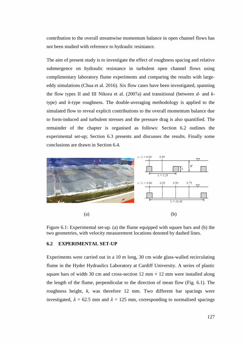
127
contribution to the overall streamwise momentum balance in open channel flows has
not been studied with reference to hydraulic resistance.
The aim of present study is to investigate the effect of roughness spacing and relative
submergence on hydraulic resistance in turbulent open channel flows using
complimentary laboratory flume experiments and comparing the results with large-
eddy simulations (Chua et al. 2016). Six flow cases have been investigated, spanning
the flow types II and III Nikora et al. (2007a) and transitional (between d- and k-
type) and k-type roughness. The double-averaging methodology is applied to the
simulated flow to reveal explicit contributions to the overall momentum balance due
to form-induced and turbulent stresses and the pressure drag is also quantified. The
remainder of the chapter is organised as follows: Section 6.2 outlines the
experimental set-up; Section 6.3 presents and discusses the results. Finally some
conclusions are drawn in Section 6.4.
(a) (b)
Figure 6.1: Experimental set-up. (a) the flume equipped with square bars and (b) the
two geometries, with velocity measurement locations denoted by dashed lines.
6.2 EXPERIMENTAL SET-UP
Experiments were carried out in a 10 m long, 30 cm wide glass-walled recirculating
flume in the Hyder Hydraulics Laboratory at Cardiff University. A series of plastic
square bars of width 30 cm and cross-section 12 mm × 12 mm were installed along
the length of the flume, perpendicular to the direction of mean flow (Fig. 6.1). The
roughness height, k, was therefore 12 mm. Two different bar spacings were
investigated, 𝜆 = 62.5 mm and 𝜆 = 125 mm, corresponding to normalised spacings

128
λ/k = 5.2 and 𝜆/k = 10.4, respectively. According to Coleman et al. (2007), the 𝜆/k =
5.2 case should be classified as transitional roughness as it is very close to the
boundary between d- and k-type roughnesses, while the 𝜆/k = 10.4 case constitutes k-
type roughness. Bed slope was fixed at 1:50 for all experiments and three flow rates
were tested for each bar spacing (Q = 1.7, 2.5, 4.0 l s-1
), giving a total of six
experimental cases. Each case had a different relative submergence, H/k, where H is
the double-averaged height of the free surface above the channel bed and the double-
averaged bulk velocity, 𝑈𝑏, ranged from 0.20 m s-1
to 0.36 m s-1
. Note that the
angular brackets and overbar have not been used for H and 𝑈𝑏 in the interest of
simplicity. Table 6.1 provides a summary of the flow conditions for each case.
Measurements of instantaneous velocity and free surface position were taken in a
section of the flume where the flow was considered to be uniform and fully-
developed. The flow was also considered to be spatially periodic with wavelength 𝜆
in the streamwise direction, that is to say the temporal mean values of all flow
variables in successive cavities between bars were considered to be the same. The
bulk Reynolds number was in the range 5700 ≤ Re ≤ 13000 and the friction
Reynolds number 𝑅𝑒𝜏 (=𝑢∗𝐻
𝜈) where 𝑢∗ is the global friction velocity based on the
bed shear stress, was in the range 1.8 x 10³ ≤ 𝑅𝑒𝜏 ≤ 3.7 x 10
3. The global Froude
number of the flows, 𝐹𝑟 = (𝑈𝑏
√𝑔𝐻), was in the range 0.38 ≤ 𝐹𝑟 ≤ 0.59; local values
based on local depths and velocities can be much higher.
A Nixon propeller meter was used to measure streamwise velocities at the channel
centreline, at two streamwise positions for the 𝜆/k = 5.2 case and four streamwise
positions for the 𝜆/k = 10.4 case. At each streamwise location the velocity was
measured at between four and eleven discrete depths, to reveal vertical velocity
profiles. At each depth measurements were taken during 120 seconds at a sampling
frequency of 1 Hz; 120 samples of instantaneous velocity were therefore available,
from which the temporal mean was calculated.
Water surface position was measured using Particle Image Velocimetry (PIV). A
Baumer TXG14F CCD camera was used in conjunction with a Polytec BUS-11

129
Wotan Flash stroboscope and a halogen lamp to capture the dynamic free surface.
Seeding particles that had the same approximate density of water, making them
neutrally buoyant, were used. The camera recorded images during 50 seconds for
each flow case, at a rate of 30 frames per second.
Figure 6.2: Variation of friction factor with relative submergence for the flume
experiments.
Table 6.1: Hydraulic characteristics of the flow conditions.
Case λ/k H/k Ub (m s-1) Re Reτ Fr Lx/H Ly/H Δx+ Δy+ Δz+
C1 5.2 2.4 0.22 5.7 x 10³ 1.8 x 10³ 0.43 4.8 2.3 69.9 66.8 35.6
C2 5.2 2.7 0.28 8.3 x 10³ 2.3 x 10³ 0.51 4.2 2.0 75.1 71.8 38.8
C3 5.2 3.3 0.36 13.3 x 10³ 3.2 x 10³ 0.59 3.4 1.6 83.8 80.2 42.8
C4 10.4 2.5 0.20 5.7 x 10³ 2.1 x 10³ 0.38 4.4 2.1 73.2 70.0 37.4
C5 10.4 3.0 0.24 8.3 x 10³ 2.8 x 10³ 0.42 3.7 1.8 80.3 76.9 41.0
C6 10.4 3.5 0.32 13.3 x 10³ 3.7 x 10³ 0.51 3.0 1.5 88.2 84.3 45.0
F1 5.2 2.7 0.28 8.3 x 10³ 2.3 x 10³ 0.51 4.2 2.0 37.5 35.9 19.1
F2 10.4 2.5 0.20 5.7 x 10³ 2.1 x 10³ 0.38 3.7 1.8 36.6 35.0 18.7
F3 10.4 3.0 0.24 8.3 x 10³ 2.8 x 10³ 0.42 3.7 1.8 40.2 38.4 20.5
D1 10.4 3.0 0.24 8.3 x 10³ 2.8 x 10³ 0.42 7.4 3.6 80.3 76.9 41.0

130
Each recording therefore comprised 1500 individual frames, which were then
transformed into binary images to smear the water surface profile using Matlab
software. These data were then averaged to give a temporal mean of the free surface
position. Figure 6.4(a) presents an individual frame from one of the cases, showing
the instantaneous free surface deformation. It should be noted that the free surface
elevation recorded by this technique was noticeably different from the elevation
observed in the centre of the channel due to Meniscus effects that were observed at
the channel sidewalls. This has the effect of thickening the appearance of the free
surface and “smearing” the profiles of the standing waves that occurred in the 𝜆/k =
10.4 cases.
In addition to the PIV measurements a point gauge was used to measure free surface
elevation at the channel centreline. Measurements were taken over a length spanning
two or more cavities, at streamwise intervals of between 2.5 mm and 10 mm. Point
gauge measurements were taken for all flow cases except C6, which was
characterised by an extremely dynamic free surface with a significant spanwise
wandering motion of the hydraulic jump, and was therefore impossible to measure
with a point gauge (Figs.0-13 in appendix I).
(a) 𝜆 /k = 5.2 (b) λ/k = 10.4
Figure 6.3: Computational domains with instantaneous free surface response (Chua
et al. 2016).
Figure 6.2 presents the variation of the friction factor, presented as (8/𝑓)1
2 and
calculated from Eq. 6.1, with relative submergence for the six cases that have been
studied. Flume data from Bathurst (1985) are included for comparison. Note that the

131
Bathurst data correspond to gravel bed roughness and were originally presented in
terms of H/D84, where D84 is the size of median axis of the bed material which is
larger than 84% of the material. The data has been replotted in terms of the
equivalent grain roughness, ks, and the relationship ks = 3.5D84 (Dietrich and Whiting
1989) has been used to equate the two measures of roughness height. With regards to
the data from the present experimental tests, the equivalent grain roughness is
assumed to be equal to the bar height (ks = k); this relationship is likely to be subject
to significant error but has been used to permit a crude comparison with the Bathurst
flume data. Interestingly the data lie within the spread of Bathurst data and agree
very well with the general trend of decreasing resistance with increasing relative
submergence. It is noteworthy that, for a given submergence, that the small bar
spacing produces less resistance than the large bar spacing.
In addition, more experiments were done to monitor the water surface profiles and to
measure the vertical velocity profiles for rough open channel flows with a bed slope
(S = 1:200) for two bar spacing (H/k= 5.2 and H/k=10.4) and three flow rates were
tested for each bar spacing (Q = 1.7 l s-1
, 2.5 l s-1
, 4.0 l s-1
) which results in different
submergence ratios, are presented in appendix I.
6.3 RESULTS AND DISCUSSION
With the help of Fig. 6.4, an instantaneous free surface profile recorded by the PIV
can be qualitatively compared to an instantaneous plot of the water surface from the
corresponding LES. Although an exact match cannot be expected due to the
Meniscus effect that affected the experiments (refer to Section 6.2), the agreement is
nonetheless very encouraging. The standing wave is very clear in both experiment
and simulation, and its height and streamwise position is very accurately predicted
by the LES.
The free surface fluctuations properties are presented including the mean and
fluctuating profiles. The longitudinal free surface profiles were recorded for twelve
experiments and compared with the numerical approach for six experiments for the
steep bed slope S = 1/50.

132
Statistical analysis of the experimental data for the longitudinal profiles was
examined. The standard deviation of the longitudinal free surface profiles were
calculated for the six relative submergences. Small free-surface fluctuations were
observed and recorded in the case of the small roughness spacing.
A significant increase in free surface fluctuation was observed in the small scale
roughness at low submergence, and the free-surface fluctuations reached a maximum
value for the large-scale roughness spacing. This maximum value increased with
increasing relative submergence, for which large standard deviations in free-surface
elevations were linked. The drawings of the standard deviation hrms/H were
explained as a non-dimensionalized relative to the uniform flow depth versus x/k.
Standard deviation results of the free surface elevations were explained in Figures
(6.5 to 6.10). For small spacing the mean free surface in all three small spacing cases
is relatively flat and standard deviation values are increased with decreasing the
submergence ratio and some undulation was observed. Upstream the bars large
magnitudes of the standard deviation were shown (see Figs. 6.5 to 6.7). For large
spacing the standard deviation values are increased and coincide with the observed
strong hydraulic jumps for all the submergence ratios (see Figs. 6.8 to 6.10).
(a) Experiment (b) LES
Figure 6.4: Visualisation of instantaneous free surface profiles, λ/k = 10.4, H/k = 2.4.
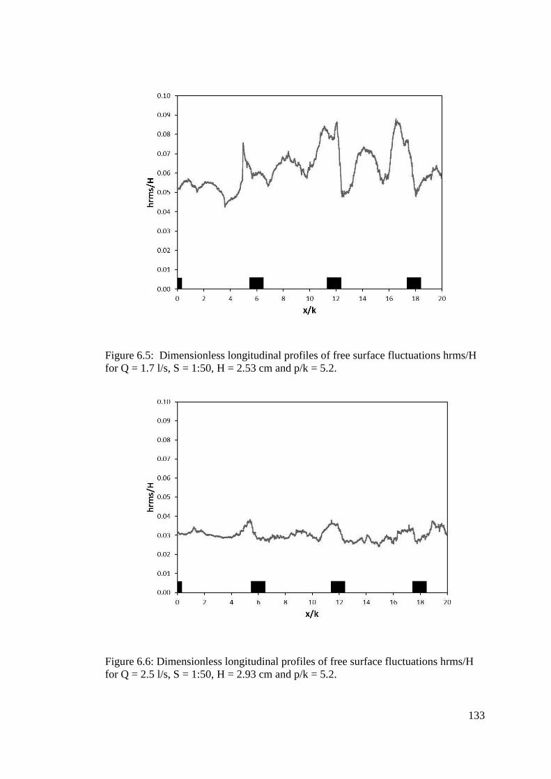
133
Figure 6.5: Dimensionless longitudinal profiles of free surface fluctuations hrms/H
for Q = 1.7 l/s, S = 1:50, H = 2.53 cm and p/k = 5.2.
Figure 6.6: Dimensionless longitudinal profiles of free surface fluctuations hrms/H
for Q = 2.5 l/s, S = 1:50, H = 2.93 cm and p/k = 5.2.

134
Figure 6.7: Dimensionless longitudinal profiles of free surface fluctuations hrms/H
for Q = 4.0 l/s, S = 1:50, H = 3.52 cm and p/k = 5.2.
Figure 6.8: Dimensionless longitudinal profiles of free surface fluctuations hrms/H
for Q = 1.7 l/s, S = 1:50, H = 2.96 cm and p/k = 10.4.

135
Figure 6.9: Dimensionless longitudinal profiles of free surface fluctuations hrms/H
for Q = 2.5 l/s, S = 1:50, H = 3.54 cm and p/k = 10.4.
Figure 6.10: Dimensionless longitudinal profiles of free surface fluctuations hrms/H
for Q = 4.0 l/s, S = 1:50, H = 4.24 cm and p/k = 10.4.

136
A more quantitative evaluation of the match between LES and experiment can be
achieved with the help of Fig. 6.11, which presents water surface profiles for the six
flow cases.
Plotted are the spanwise mean of the temporal mean water surface predicted by the
LES and the means that were measured using PIV and the point gauge. The
agreement between experiments and LES is particularly good for the small spacing
(λ/k = 5.2) cases.
The mean free surface in all three small spacing cases is relatively flat, although
some undulation is noticeable in the lowest submergence case (Fig. 6.11(a)). In fact
two unsteady undular jumps are present in this flow case, slightly upstream of the
bars. These jumps establish and disestablish periodically. In the large spacing cases
well defined hydraulic jumps are visible between the bars, where the local Froude
number approaches unity and the flow becomes critical.
For the low submergence, large spacing case (Fig. 6.11(d)) the elevation predicted
by LES C4, is noticeably higher than the measured elevations. The agreement in the
medium submergence, large spacing case (Fig. 6.11(e)) appears to be very
convincing.
As stated in Section 6.2, point gauge measurements were not possible in the high
submergence, large spacing case (Fig. 6.11(f)) due to the extremely dynamic nature
of the surface and very significant spanwise components of motion that were
observed in the undular jump. This spanwise behaviour is also the reason for the
poor agreement between the LES and the PIV in this case. Further validation of the
LES is provided by vertical profiles of the spanwise and temporal mean of the
streamwise velocity from the LES in Figs. 6.12 and 6.13, alongside the experimental
data, which were recorded at the channel centreline using the Nixon propeller meter.

137
Figure 6.11: Longitudinal profiles of temporal and spanwise mean free surface
elevation for three approaches (experimental using PIV, experimental using point
gauges and numerical using LES).
The measurement locations are illustrated in Fig. 6.1: two profiles were measured in
the 𝜆/k = 5.2 cases and four were measured in the 𝜆/k = 10.4 cases.
(a) H/k = 2.4 (b) H/k = 2.7 (c) H/k = 3.3
Figure 6.12: Vertical profiles of mean streamwise velocity: λ/k = 5.2 (Chua et al.
2016).

138
Figure 6.13: Vertical profiles of mean streamwise velocity: λ/k = 10.4 (Chua et al.
2016).

139
In general, the LES data from all six cases show good agreement with the
experiments. It should be noted that the experimental data points at z/k = 1 have been
given a filled symbol to highlight the fact that these measurements are possibly less
reliable than the others: these points are located in the shear layer at the top of the
roughness elements, and it is known that the Nixon probe is not well suited to
regions of high shear and rotation. In the three 𝜆/k = 5.2 cases significant negative
velocity is observed close to the bed in the middle of the cavity, while there is
relatively little streamwise variation in the profiles above the roughness top,
indicating a skimming type flow with stable or quasi-stable recirculations in the
cavities. In each of the larger spacing cases a region of negative mean velocity is
observed near the bed at 𝑥/k = 0.25 but not at 𝑥/k = 0.5, suggesting that reattachment
to the bed occurs in the upstream half of the cavity.
A more detailed understanding of the flow field can be reached by considering the
contours of spanwise and temporal mean streamwise velocity that are presented in
Fig. 6.14. For the small spacing, low submergence case (Fig. 6.14(a)) the contours
reveal that, although the mean water surface is relatively flat, significant velocities
are experienced above it. This is due to the periodic establishment and
disestablishment of undular hydraulic jumps just upstream of the bars. When such
jumps are present the local water surface rises and a non-zero velocity is experienced
in the near surface region, contributing to the non-zero mean. Importantly, Fig.
6.14(a) also shows significant streamwise variation of velocity throughout the depth,
with local acceleration and deceleration occurring between and above the bars,
respectively. In contrast, the two deeper small spacing cases (Figs. 6.14(b) and (c))
are characterised by relatively little streamwise variation of velocity above the bars.
The plots for the large spacing cases, Figs. 6.14(d)-(f), reveal regions of locally-
accelerated flow that give rise to local Froude numbers close to 1.0, which in turn
lead to dramatic deformations of the water surface and the formation of the hydraulic
jumps. The hydraulic jumps are characterised by a small region of negative
streamwise velocity produced by the plunging and breaking motion of the standing
waves. The plots also confirm the presence of a mean recirculation bubble in the

140
wake of the upstream bar, as well as a small corner vortex at the leading face of the
downstream bar.
Figure 6.14: Contours of the temporal and spanwise mean normalised streamwise
velocity (Chua et al. 2016).
Figure 6.15 presents contours of the spanwise and temporal mean of the
streamfunction, 𝜓, for the six cases. Note that positive streamfunction is denoted by
solid contour lines while dashed lines denote negative streamfunction. The plots
confirm the observations noted above regarding the velocity profiles and contours,
and also offer some important additional insights. Firstly, the plots clearly show that
the close spacing cases are characterised by large recirculations in the cavities, while
the mean flow does reattach to the bed in the large spacing cases. The contours also
confirm that the 𝜆/k = 5.2 cases should indeed be classified as transitionally rough,
rather than d-type, as the streamlines in the shear layer do not quite connect the top
of the elements to create a pseudo-smooth wall, as in Stoesser and Rodi (2004) for
example.

141
In fact the 𝜓 = 0 contour impinges on the leading faces of the roughness elements,
indicating that some form drag will be experienced at the top of the bars and flow in
this region will undergo some degree of unsteadiness. Therefore, although the
velocity profiles in Fig. 6.12 suggested relatively little streamwise variation in the
streamwise velocity, the mean flow field above the roughness crests is not quite
homogeneous, as would be the case in a true skimming or psuedo-smooth wall flow.
Instead, it can be considered that the bars present a psuedo-rough wall at the crest
height, resulting in the streamwise undulations in the streamfunction contours that
are visible in the plots.
The lowest submergence case (Fig 6.15(a)) in particular reveals a somewhat wavy
streamfunction field and suggests the presence of a fairly strong undular jump at the
free surface as discussed above with reference to the contours of mean streamwise
velocity. In the 𝜆/k = 10.4 cases the mean flow reattaches to the bed between the bars
and can be unequivocally categories k-type roughness. The length of the mean
recirculation bubble decreases as submergence increases.
Figure 6.16 presents contours of the spanwise and temporal mean of the turbulent
kinetic energy, tke, normalized on the square of the global friction velocity 𝑢∗, for
the six flow cases. The mean free surface position is overlaid for reference. A highly
turbulent shear layer is present above the roughness crests in the small spacing cases,
and in the two higher submergence flows for that spacing (Figs. 6.16(b) and (c))
there appears to be relatively little turbulent activity near the surface.
The low submergence, small spacing case (Fig. 6.16(a)) displays a different
character, however, showing high levels of turbulent energy near the surface and a
noticeably less turbulent shear layer near the roughness crests compared to the higher
submergence cases.

142
Figure 6.15: Contours of the temporal and spanwise mean of the streamfunction
(Chua et al. 2016).
The turbulent energy experienced at the free surface is produced by the unsteady
undular jumps that were indicated in the corresponding streamfunction plot (Fig.
6.15(a)) and involve the generation of large scale turbulent structures that are
convected downstream with the mean flow. The complexity of the flow in the large
spacing cases is evident from the tke plots. Each case displays a very localised peak
in turbulent kinetic energy at the location of the hydraulic jumps that occur between
the bars.
All cases under investigation are expected to belong to the class of intermediate
submergence (type II) flows as defined by Nikora et al. (2007a). The boundary layer
is therefore not expected to comprise the logarithmic layer that occurs in smooth bed
and high submergence rough bed flows.

143
Figure 6.16: Contours of the spanwise mean normalised turbulent kinetic energy
(Chua et al. 2016).
Figure 6.17 presents profiles of the double-averaged streamwise velocity, ⟨𝑢+̅̅̅̅ ⟩ =
(⟨�̅�⟩/𝑢∗), where 𝑢∗ is the global shear velocity, the overbar denotes temporal
averaging and the triangular brackets denote spatial averaging. In all cases the spatial
averaging operation has been performed over the entire computational area. The
wall-normal distance in the vertical direction, 𝑧+, is chosen for the x-axis, following
the format of the well-known Clauser plot. Cases with the same flow rate (Table 6.1)
and therefore similar relative submergence have been plotted together to enable
meaningful comparisons. The plots do indeed confirm that no genuine logarithmic
layer can be defined for any of the cases, with the possible exception of the high
submergence, small spacing case (Fig. 6.17(c)), which does comprise a straight
section that extends over a significant section of the water depth and could be
considered to be a transitional type I-II flow.

144
(a) (b) (c)
Figure 6.17: Variation of double averaged streamwise velocity with wall-normal
distance (Chua et al. 2016).
Figure 6.17 shows that peak double-averaged velocity is significantly higher, and the
velocity gradient significantly steeper, in the small spacing cases compared to the
large spacing cases. This is due to the constriction on the bulk flow that is imposed
by the bars. The pseudo-rough wall, discussed above, that forms at the roughness
crests acts to reduce the overall cross-sectional area available to the bulk flow,
thereby increasing the velocity in this region relative to the equivalent large spacing
case. Note also that the recirculating cavity flow in the small spacing cases produces
a significant region of negative double-averaged velocity below 350 ≤ 𝑧+ ≤ 500,
whereas in the large spacing case only a very small amount of negative flow is
observed.
Vertical profiles of normalized spatially-averaged Reynolds shear stress, ⟨𝑢′𝑤′̅̅ ̅̅ ̅̅ ⟩, are
shown in Fig. 6.18. The plots reveal markedly different trends for the small and large
spacing cases. For the two small spacing, high submergence cases (Figs. 6.18(b) and
(c)), ⟨𝑢′𝑤′̅̅ ̅̅ ̅̅ ⟩, increases approximately linearly with distance from the free surface,
reaching a peak at the height of the roughness crests. This is consistent with other
studies of turbulence in rough-bed flows (Bomminayuni and Stoesser 2011, Manes
et al. 2007, Singh et al. 2007, Stoesser and Nikora 2008). Below the roughness crests
⟨𝑢′𝑤′̅̅ ̅̅ ̅̅ ⟩ decreases approximately linearly from the peak until it reaches zero at the
channel bed, an observation also made by Stoesser and Nikora (2008). In the
corresponding large spacing cases the variation of the Reynolds stress with height is

145
clearly not linear, either above the crests or below, and displays significant curvature
throughout the depth.
Figure 6.18: Vertical profiles of spatially-averaged Reynolds stress (Chua et al.
2016).
An interesting feature of the Reynolds stress variation in all three large spacing
cases, and also in the small spacing, low submergence case, is the portion of
significantly positive ⟨𝑢′𝑤′̅̅ ̅̅ ̅̅ ⟩ that occurs close to the water surface. These positive
stresses are the result of turbulence production at the unsteady surface, which has
already been discussed with reference to the tke contours (Fig. 6.16). The
implications of the positive stresses for the streamwise momentum balance and
overall hydraulic resistance in the channel can be appreciated by considering Eq. 6.2,
which splits the friction factor into additive constituents. The equation indicates that
negative spatially-averaged Reynolds stress acts to adds to the friction, while
positive stress should acts to reduce it. These results therefore suggest that in open
channel flows with unsteady, turbulent free surfaces, turbulent stresses near the
surface may produce negative streamwise drag.
Figure 6.19 presents vertical profiles of the spatially-averaged form-induced shear
stress,⟨�̃��̃�⟩, which arises from spatial fluctuations in the mean flow field due to the
spatially heterogeneous nature of the rough bed. Examination of Eq. 6.2 reveals that,
as with the Reynolds shear stress, a negative spatially-averaged form-induced stress
will contribute positively to the overall hydraulic resistance in the channel. The plots
show that in all cases ⟨�̃��̃�⟩ increases non-linearly with distance from the bed until it
reaches a peak at the height of the roughness crests.

146
(a) (b) (c)
Figure 6.19: Vertical profiles of spatially-averaged form-induced stress (Chua et al.
2016).
This is consistent with previous studies by Manes et al. (2007) and Stoesser and
Nikora (2008), for example, who also showed that ⟨�̃��̃�⟩ then decreased fairly rapidly
above the roughness crests and remained at zero for the upper part of the water
column. Figs 6.19 (b) and (c) confirm that this general trend is also observed in the
present study for the two small spacing, high submergence cases. These two cases
can therefore be classified as type II (intermediate submergence) flows, since there
clearly exists a portion of the depth in which form-induced stresses are not
significant. In the other four cases, however, significant non-zero form-induced
stresses are observed throughout the whole water depth, indicating that the form-
induced sub-layer extends all the way to the free surface. These cases therefore
belong to the class of type III (low submergence) flows. Furthermore, the most
striking features of Fig. 6.19 are the very large negative stresses in the near-surface
region for the four cases in which the surface was observed to be turbulent and
unsteady. This result indicates that the standing wave-type responses that were
observed at the free surface will make a significant contribution to the overall
resistance in the flow.
It is noteworthy that the magnitudes of these negative near-surface peaks in form-
induced stress are always larger than the corresponding positive Reynolds stress
peaks that are observed in the same region (Fig 6.18): the net contribution of the free
surface response to the overall drag is therefore always positive, as confirmed by
Fig. 6.20, which presents profiles of the combined (form-induced + Reynolds) stress.

147
The stress variation above the roughness crests is shown to be approximately linear,
even in the large spacing cases in the near-surface region. The plots suggest that
extrapolation of the slope from the height of the roughness crests to the x-axis would
result in a stress of approximately -1, which is consistent with other studies of flows
over rough beds, for example in Manes et al. (2007). The reason that the stress does
not reach this value at the bed is the dominance of the form drag in the interfacial
sub-layer (0 ≤ z ≤ k), which produces an approximately linear reduction in the
contribution of Reynolds and form-induced stresses until they disappear completely
at the bed.
(a) (b) (c)
Figure 6.20: Vertical profiles of combined spatially-averaged Reynolds and form-
induced stress (Chua et al. 2016).
Figure 6.21 presents vertical profiles of the span and temporal mean of the pressure
differential across a single bar, (𝑝𝑢 − 𝑝𝑑) where 𝑝𝑢 and 𝑝𝑑 are the pressures on the
upstream and downstream faces using two different normalisations. Only the
interfacial sub-layer (0 ≤ z ≤ k) is considered. The pressure differential is a measure
of the pressure or form drag acting on the individual bars, which is simply the
difference between the integrated pressures on each face.
In Fig. 6.21(a) the differential is normalised on 1
2𝜌𝑈𝑏
2, giving a pressure coefficient.
The plot shows that the pressure differential, and therefore the form drag, acting on a
single bar is consistently higher in the large spacing cases compared to the small
spacing cases. The form drag also increases with decreasing relative submergence.

148
(a) (b) (c)
Figure 6.21: Pressure differentials between upstream and downstream faces of a
single bar. Note that in plot (b) the pressure force has been multiplied by 2 to
account for the presence of two bars in the streamwise direction (Chua et al. 2016).
These two findings are consistent with the trends that are illustrated in the plot of
friction factor versus relative submergence (Fig. 6.2), and suggest that the form drag
is the dominant contributor to overall drag in all cases. The increase in form drag
when submergence is reduced is also consistent with the trend for decreasing
recirculation bubble length that was observed in the plots of mean streamfunction
(Fig. 6.15). Figures 6.21 (b) and (c) present the pressure differential as a force,
𝐴𝑏𝑎𝑟(𝑝𝑢 − 𝑝𝑑) where 𝐴𝑏𝑎𝑟(= 𝑘 × 𝐿𝑦) is the cross-sectional area presented to the
flow by one bar, normalised on the global shear force, 𝐴𝑏𝑎𝑟(𝑝𝑢 − 𝑝𝑑), where
𝐴𝑥𝑦(= 𝐿𝑥𝐿𝑦) is the planar area on which the shear stress acts. The plots show that
the form drag contributes close to 100% of the overall drag in the interfacial sub-
layer, and in the small spacing cases (Fig. 21(b)) even contributes more than 100%
very close to the bed. This result is explained by the presence of strong recirculation
zones with negative flows in the cavities between bars, leading to negative shear
stresses that in turn oppose the overall drag force. In order to balance these negative
contributions to the overall shear force, some extra form drag must be present close
to the bed. In the large spacing cases the form drag is approximately uniform up to a
height of approximately 0.8k, after which it decreases fairly rapidly.

149
6.4 CHAPTER SUMMARY
Complementary flume experiments of turbulent open channel flows over bed-
mounted square bars at intermediate submergence have been presented. In total six
flow cases were investigated, comprising two roughness spacings that correspond to
transitional and k-type roughness and three flow rates. The bed slope was held
constant for all cases, and relative submergence therefore increased with flow rate. In
the experiments the water surface was observed to be very complex and turbulent for
the large spacing cases, and comprised a single hydraulic jump between the bars.
The streamwise position of the jump varied between the cases, with the distance of
the jump from the previous upstream bar increasing with flow rate. The free surface
was observed to be less complex in the small spacing cases, particularly for the two
higher flow rates, in which case the flow resembled a classic skimming flow. The
Darcy-Weisbach friction factor was calculated for all six cases from a simple
momentum balance, and it was shown that for a given flow rate the larger bar
spacing produces higher resistance.
The predictions of the LES that was achieved by Chua et al. (2016) for the flow over
square ribs are shown in good agreement with the experiments in terms of mean free
surface position and mean streamwise velocity. The position of the hydraulic jumps
was well represented. Contours of spanwise and temporal mean streamlines revealed
that the small spacing cases were characterised by classic cavity flow with a quasi-
rough wall presented at the height of the roughness crests. In the large spacing cases
the length of the mean recirculation bubble was observed to decrease with relative
submergence.
Analysis of spatially-averaged Reynolds shear and form-induced stress profiles in
the context of the friction factor equation proposed by Nikora (2009) revealed that,
in cases in which significant turbulence production occurs at the free surface, the
Reynolds stress may be positive near the surface and can therefore act to reduce the
overall drag experienced by the flow. Secondly, vertical profiles of form-induced
stress revealed significant negative peaks in these complex near-surface regions,
resulting from spatial fluctuations in the mean flow due to the presence of hydraulic
jumps. The magnitudes of these negative form-induced stresses are larger than those

150
of the positive Reynolds stresses, and therefore act to produce a net contribution to
the overall drag at the free surface. The form drag acting on individual bars was
analysed and it was shown that the contribution of form drag is larger in the large bar
spacing and increases with decreasing relative submergence.

151
CHAPTER SEVEN
SUMMARY, CONCLUSIONS AND
FUTURE WORK

152
7 SUMMARY, CONCLUSIONS AND FUTURE WORK
7.1 INTRODUICTON
This chapter presents a summary of research findings, conclusions and future
research that is mainly considered as follows:
Section 7.2 summarises devices and equipment that were used to satisfy the research
objectives. Section 7.3 presents the findings of the research in open channels, while
section 7.4 summarises the research findings on compound channel flows.
Recommendations for future research are provided in section 7.5.
7.2 SUMMARY OF RESEARCH FINDINGS
This study aimed of investigating the hydrodynamics of large-scale roughness in
open channel flows in different subject areas. Attention was focused on the free
surface dynamics at steady uniform flow conditions. Single and compound open
channel cross sections were considered for the laboratory experiments. Various
devices and equipment were utilized; Nixon probe velocimetry was used for point
velocity measurements; point gauge to measure the water depths; particle image
velocimetry to monitor and track video images of water surface profiles over rough,
steep open channel flow; and a thermal camera was used to capture temperature
distribution at the water surface between the main channel and the floodplain in
compound open channel flows.
Water surface profile response in the presence of a hydraulic structure, such as
lateral channel constriction and submerged bridge constriction as investigated. Flume
experiments involved measuring flow depths at different locations in the longitudinal
and the lateral directions from the constriction to enrich our understanding on flow
dynamics in the presence of such hydraulic structures. This study was achieved in a
glass sided flume with a smooth bed of 30 cm width set at a bed slope of 1/2000.
Two physical man-made structure models were selected as the lateral constriction
and bridge overtopping obstructions. Longitudinal and lateral water surface profiles
were examined experimentally and numerically using LES (Kara et al. 2014, Kara et
al. 2015) for both constrictions.
153
Hydrodynamics of one-line vertically oriented cylinders located at the centre of the
30 cm wide flume was considered focusing on drag coefficient calculations. Drag
coefficients were calculated and then compared with different analytical expressions
derived for an array of vegetation. Experiments were performed to measure the
stage–discharge behaviour of open channel flow through one line of vertically-
oriented circular rods which mimics in-line vegetation. Two bed slopes were used,
along with a range of rod diameters which yielded different spacings between
cylinders.
Hydrodynamics of compound channels with vegetated floodplain were investigated.
Rigid emergent cylindrical rods were used to simulate the vegetation. Two
vegetation configurations – wholly vegetated floodplain and one-line vegetation
were considered and the hydraulic properties are compared to those of a smooth
unvegetated compound channel. Particular attention was given to the effect of
vegetation density on the rating curve, drag coefficient and spanwise profiles of
streamwise velocity. Flow resistance was estimated using the approach introduced
by Petryk and Bosmajian and the results were in agreement with other experimental
studies. It was shown that the vegetation configuration significantly influences the
velocity in the main channel and in the case of one line vegetation the floodplain
velocity is higher than for unvegetated channel for a given flow rate. Spanwise
velocity profiles exhibit markedly different characters in the one line and wholly
vegetated configuration.
Free surface flow over square bars at low and intermediate relative submergence was
achieved with a complimentary series of flume experiments of flow over square bars
of dimensions 12mm x 12mm x 300mm that were attached along the entire flume
length with two spacing (pitch to pitch) of 6.25 cm and 12.5 cm. Experiments were
carried out with a range of flow rates of 1.6 l s-1
to 10 l s-1
with flume bed slopes of
0.001, 0.005, and 0.02 with two roughness spacing of 5.2 and 10.4. Monitoring water
surface profiles over rough beds was carried out using a PIV system. Particle image
velocimetry was used to capture video images to monitor the free surface profiles of
the flow over the square bars for two bed slopes (1:50 and 1:200), two roughness
spacing (H/k = 5.2 and H/k = 10.4) and three flow rates (Q= 1.7, 2.5 and 4.0 l s-1
).

154
The results of the longitudinal water surface profiles are expressed as mean-averaged
of 1500. Point gauge measurements were also carried out between two bars in the
experiments for the bed slope 1:50. Measurement of time-averaged longitudinal
stream-wise velocities of a steady, fully developed flow in rough open channels were
carried out for the entire water depth in the inner and the outer regions of the
turbulent boundary layer over a rough surface. With bed slope (S = 0.02) and
roughness spacings (λ/k = 5.2 & 10.4), velocity measurements for large roughness
spacing (λ/k = 10.4) were taken at four sections, over the rib and three downstream
of the rib, which showed that the vertical point velocity values over the mid width of
the rib element are less than that at a section 3.125 cm down-stream of the rib
centreline for all the flow rates used. As the roughness elements are closer, i.e. λ/k =
5.2, two profiles were measured. The aim was to explore the effect of flow depth and
roughness spacing on free surface flow dynamics at low and intermediate relative
submergence. Variation of friction factor with relative submergence for the flume
experiments was compared with Bathurst (1981 and 1983)’s equation.
Dynamics of the water surface at the interface between the main channel and the
floodplain was assessed for a compound channel section using a thermal camera SC
640 with two vegetation configurations - wholly vegetated floodplain and one-line
vegetation for the aims; (i) to visualize and evaluate such technique in capturing
thermal shear layers at the interface between the main channel and the floodplain, (ii)
to understand the effect of vegetation density and configuration and flow depth on
the thermal shear layer thickness and its evolution along the floodplain-main channel
edge in the compound channel.
A review of the main results obtained and conclusions derived from this study are
presented as follows:
7.3 CONTRIBUTIONS TO OPEN CHANNEL HYDRODYNAMICS
RESEARCH
Considering the aims outlined at the beginning of this chapter, the achievements of
this study can be classified into three major subject areas which are (a) water surface
response to flow through bridge openings, (b) hydrodynamics of one-line vegetation

155
in open channel flows and (c) free surface flow over square bars with low and
intermediate relative submergence.
(a) Water surface response to flow through bridge openings
With the lateral constriction, longitudinal water depth measurements showed that the
water backed up quite significantly upstream of the structure. A short distance
upstream of the structure, the flow starts to accelerate and the water surface drops
rapidly and significantly. The flow creates a very distinct dip in the area of localised
recirculation as a result of flow separation at the leading edge of the constriction.
The water surface recovers markedly approximately half way through the
constriction in the form of a standing wave. Towards the end of the constriction, the
water surface drops further quite significantly. The flow downstream of the
constriction is subjected to a large, very shallow recirculation zone just behind the
abutment, which contracts and accelerates the flow.
The cross-sectional profiles downstream of the constriction exhibit a very significant
jump in the water surface. The recirculation zone downstream of the constriction is
at a significantly lower elevation than the rest of the channel. The water that rushes
out of the constricted area has a significant amount of stream wise momentum
prohibiting the filling of the recirculation zone with fluid.
The result of LES shows reasonable agreement with the experimental data for both
the longitudinal and lateral water surface profiles. However, with the longitudinal
profiles in close proximity to the structure, LES shows a weak agreement between
the simulated and the measured values due to the lack in mesh resolution of the
simulation.
With the bridge overtopping simulation, three types of flows were monitored;
subcritical flow upstream of the bridge, critical flow state on the deck of the bridge
due to the deck acting as a broad crested weir, and supercritical flow downstream of
the deck. The flow recovers to subcritical in the form of an undular hydraulic jump.
The simulated longitudinal water surface profiles are in good agreement with the
measured data. However, an inconsistency between the simulation and the observed

156
data was found just upstream of the bridge because the deck of the numerical
simulation is slightly higher than the one used in the experiment. The discrepancy
between the numerical and the observed values belongs to the difficulty of point-
gauge measurements at high turbulence.
Lateral water surface profiles were simulated in good agreement with the observed
data, except for the profiles upstream of the bridge; the numerically predicted
profiles are slightly higher than the observed ones.
(b) Hydrodynamics of one-line vegetation in open channel flows
For a series of uniform flows the drag coefficient was calculated based on the
measured uniform flow depth and under consideration of the bed friction. Then the
most prominent empirical equations for calculating the drag coefficient, CD, of
vegetation have been employed to predict CD for the experiments of in-line
vegetation (Tanino and Nepf 2008, Kothyari et al. 2009, Cheng and Nguyen 2011,
Cheng 2013). Tanino and Nepf’s and Kothyari’s equations consistently overestimate
the measured drag coefficients but match the overall trend of an increase of CD with
increasing stem Reynolds number. Cheng’s and Cheng and Nguyen’s expressions
overestimate vegetation drag for low to medium values of ReD whilst a good match
has been achieved for the higher stem Reynolds numbers. On the other hand the
latter two expressions do not reflect the trend of an increase of CD with increasing
stem Reynolds number. The results show that varying the diameter of the rigid
emergent vegetation affects significantly flow resistance.
(c) Free surface flow over square bars with low and intermediate relative
submergence
From the experiments it is demonstrated that for a fixed rib height, increasing the
flow depth resulted in a decrease of the friction factor. For a constant bed slope,
increasing the spacing between rib elements causes an increase in the friction factor,
while for a constant roughness spacing, increasing the bed slope causes an increase
in friction factor.

157
The friction factor was compared with the flume data from Bathurst (1985). The data
lie within the spread of Bathurst data and agree very well with the general trend of
decreasing resistance with increasing relative submergence.
It has been shown that for a given discharge (Q) and roughness spacing (λ/k), the
water depth (H) decreases as the bed slope (S) increases, whilst increasing the
roughness spacing causes an increase in the water depth for all the selected bed
slopes.
The impact of roughness spacing on the dynamics of the free surface flow is such
that for a constant roughness spacing of λ/k = 10.4 and a bed slope of 0.02, strong
well defined hydraulic jumps with air bubbles between the bars were observed, while
weak hydraulic jumps and no trace of the air bubbles were in existence for the same
bed slope with roughness spacing λ/k = 5.2. This ensures that roughness spacing
plays a crucial role in the configuration of the water surface profile and then on the
friction factor. The free surface was observed to be less complex in the small spacing
cases, particularly for the two higher flow rates, in which case the flow resembled a
classic skimming flow.
The mean free surface in all three small spacing submergence ratios is relatively flat,
while some undulation is observable in the lowest submergence case. For the large
spacing submergence cases, increasing the submergence ratio, H/k, noticeable effects
the free surface topology.
The results of the spanwise mean of the temporal mean water surface was also
predicted by the LES (Chua et al. 2016) and the mean water surface that were
measured using PIV and the point gauge were compared and showed good
agreements. The agreement between experiments and LES is particularly good for
the small spacing (λ/k = 5.2) cases.
Velocity measurements showed that velocity profiles are closer to each other, or
have the same values at the location over the rib element section and in the section
down-stream of the rib centreline at a distance of 3.125 cm. Vertical velocity profiles
with roughness spacing of 10.4 and a bed slope (S = 0.005) in the four sections
showed that, the curves are of much smaller than that with the bed slope of 0.02.

158
However, these velocity profiles coincide in the case of bed slope of 0.005 and
roughness spacing of 5.2 as shown in Fig. 0-16 in Appendix I.
Large-eddy simulations provided contours of mean velocity, mean streamfunction
and turbulent kinetic energy and revealed the effect of the roughness geometry on
the water surface response. For the low submergence cases dynamic responses were
observed at the surface, including the presence of hydraulic jumps which contribute
significantly to the overall streamwise momentum balance. Analysis of spatially-
averaged Reynolds shear and form-induced stress profiles in the context of the
friction factor equation proposed by Nikora (2009) revealed that, in cases in which
significant turbulence production occurs at the free surface, interesting results, the
Reynolds stress may be positive near the surface and can therefore act to reduce the
overall drag experienced by the flow. Secondly, vertical profiles of form-induced
stress revealed significant negative peaks in these complex near-surface regions,
resulting from spatial fluctuations in the mean flow due to the presence of hydraulic
jumps. The magnitudes of these negative form-induced stresses are larger than those
of the positive Reynolds stresses, and therefore act to produce a net contribution to
the overall drag at the free surface. The form drag acting on individual bars was
analysed and it was shown that the contribution of form drag is larger in the large bar
spacing and increases with decreasing relative submergence.
7.4 CONTRIBUTIONS TO COMPOUND OPEN CHANNEL FLOW
RESEARCH
At shallow, uniform flow a clear impact of floodplain vegetation on the rating curve
is found for all vegetation densities and configurations.
The inclusion of a wholly-vegetated floodplain produces a marked increase in water
depth compared to the unvegetated case for a given flow rate. Increasing the
vegetation density, results in further increase in water levels. The water level
increases with flow rate in all cases appears to increase linearly with flow rate when
the floodplain is vegetated contrary to the case for the unvegetated channel case.

159
The inclusion of one-line vegetation at the interface between main channel and
floodplain produces a much smaller increase in water depth compared to the wholly-
vegetated floodplain cases. That is because flow blockage, for the one-line case is
naturally much smaller than in the full-vegetated case. Water depth is noticeably
more sensitive to changes in length-to-diameter for one-line vegetation than to
changes in vegetation density for a wholly-vegetated floodplain.
Estimation of the drag coefficient for the wholly vegetated floodplain which is based
on equating the gravitational force to the drag force exerted by the vegetation
elements was analysed and compared with the most applicable empirical equations.
These equations are Tanino and Nepf (2008), Kothyari et al. (2009) and Cheng and
Nguyen (2011). The experimental results showed good agreement with these
equations. The drag coefficient displays a high degree of sensitivity to changes in
both Reynolds number and vegetation density.
Based on point velocity measurements, for the wholly-vegetated and unvegetated
floodplains the spanwise profiles follow an S-shaped curve but for one-line
vegetation the profiles exhibit a distinct dip at the interface between the main
channel and the floodplain. Lateral velocity profiles showed two sections of uniform
velocity namely vegetated and open channel sections and transitional region. The
highest velocity differences between the main channel and the floodplain are
observed in the presence of roughness differences between these two sections. Flow
velocity above a wholly-vegetated floodplain is noticeably lower than that above an
unvegetated floodplain
With a one-line vegetation configuration, strong velocity gradients were seen in the
rod area which means that these rods suppress transferring momentum from the main
channel to the floodplain for all rod diameters and flow rates, while these velocity
gradients were clearly shown to be of less magnitude with the wholly vegetated
floodplain. The inclusion of one-line vegetation produces higher velocities above the
floodplain compared to the unvegetated case.
Fully turbulent developed flows were observed for the compound channel sections
with vegetated and non-vegetated floodplains.

160
Using image processing techniques together with Matlab software allows
visualisation of the shear layer that forms at the interface between the main channel
and the floodplain of a compound channel flow. The thermal shear layer at the
interface of the vegetated floodplain was shown to be influenced by the flow depth
variation and with vegetation density and distribution in comparison to the non-
vegetated case due to the drag by vegetation. In addition, for the vegetated floodplain
the penetration thickness inside the main channel is greater than that on the
floodplain. However, for the non-vegetated floodplain, the penetration thickness was
observed to be of equal magnitude inside the main channel and the floodplain and
influenced by the flow depth variation. For a given vegetation density on the
floodplain, increasing the discharge leads to an elongated shear layer. With a one-
line of vegetation, the biggest diameter results in the shortest shear layer elongation,
while for the wholly vegetated floodplain, the highest vegetation density results in a
wider shear layer distribution.
Time-averaged temperature distribution results were analysed and examined to
clarify how temperature dissipates longitudinally and transversely along the stream-
wise direction (x-y plane). A steep variation of the temperature values was
monitored in the lateral direction for all the tests and a gradual variation of the
temperature was observed in the first quarter of the shear layer length in the stream-
wise direction. Steep variation of water temperature was observed in all the
experiments. The rapid decrease in water temperature from the peak to a value of 23
(laboratory water temperature) refers to the turbulent mixing between the compound
channel sections.
Inferring flow properties from the thermal camera temperature series were achieved
for the wholly vegetated floodplain to characterize the development of eddies in the
wake of the rods. Results showed that two types of vortices (shear layer vortices and
von-Karman street vortices) can be distinguished. Shear layer vortices were
monitored at the outer edge of the rods, while von Karman vortices are tracked
behind the rod with a counter rotating vortex pair. With a rod diameter of D = 2.5 cm
the von Karman vortices were shown, while with rod diameter of D = 5.0 cm the
interaction of the stream-wise velocity and span-wise velocity between the rods
inhibit these types of vortices. More details about the eddy properties were analysed

161
from the five selected points in the wake region and showed successive peaks along
the time series curve. Fast Fourier transform of the time series of temperature for the
selected five points showed the energy of the eddies is small at high frequency, while
for small frequencies there are large eddies.
Mass and momentum transfer between the main channel and the floodplain due to
the effects of the transverse depth variation and the variation of bed roughness. This
results in velocity gradients between the main channel and the floodplain and
expressed in the lateral distribution of the depth averaged-velocity diagrams.
7.5 RECOMMENDATIONS FOR FUTURE RESEARCH
This research requires further assessment and additional research of:
Dynamics of shear layers in compound channel flows
In order to further understand the dynamics of shear layers at the interface
between the main channel and the floodplain in compound channel flows,
more experiments are needed based on particle image velocimetry. These
measurements may focus on the instantaneous velocity at the water surface
between the main channel and the floodplain to enrich our understanding of
flow dynamic properties of flow in compound channels. Investigating the
flow properties at the water surface enable comparison between the shear
layers that can be extracted by the thermal camera with the PIV results and to
explore more details about the vortices that are generated behind the
neighbouring cylinders located on the floodplain.
Using the PIV in tracking the water surface shear layers (vortices) enables us
to visualize and evaluate the impact of vegetation density on the interaction
of the vortices that cannot be explained by the thermal camera.
Flow dynamics in the presence of one-line vegetation are needed. The
influence of vegetation elements on each other may be explained by the
shading factor, SF. The impact of the shading factor has been explained by
Noat et al. (1996) expression and Nepf (1999) diagram. These are not enough
to describe the impact of vegetation elements by the shading factor. This is

162
partly due to limited literature. More experiments are therefore required to
investigate the impact of shading factor in the presence of one-line of
vertically-oriented circular rods at different aspect ratios. The rod diameters
will be investigated both in a single and compound channel flows at a
different locations from the sidewall of the stream.
Free surface flow over square bars with low relative submergence
Accurate estimation of flow resistance in mountain streams requires adequate
evaluation of the resistance imposed by bed morphology on the flow. One of
the scenarios that should be studied in the hydraulic laboratory is to use more
natural 3D large-scale roughness in different arrangements and with different
concentrations. Turbulence characteristics of the flow in the area of the rough
elements can be extracted by PIV system to measure the flow velocity field.
This enables us to understand the effects of bed roughness arrangement and
relative submergence on the flow properties.
Water surface profile over rough beds can be monitored using a thermal
camera and a tracer of hot water. An adequate number of video files are
required to capture the water surface profile of the running water from the
flume sidewall. The tracer can be applied by heating the running water to a
degree more than that of the hydraulic laboratory environment.
Thermal camera can be used to deduct many physical hydraulic phenomena,
for example, kolk boils at the water surface in rough open channels, and kolk
boils in the presence of lateral constriction such as groins. In addition, PIV
can be used to extract more details about these vortices that are generated due
to the exchange of momentum between the roughness layers and the
overlying flow.
Water surface response to flow through bridge openings
The use of a submerged bridge can be expanded for more case studies. The
bridge opening was considered, in such a way that 74% of the flow is run
under the deck. The flow running under the deck can be examined with
163
different gate openings, such as 50%, 60% and 90%. In addition, an elliptical
pier can be used instead of rectangular one.

164
PUBLICATIONS RELATED TO THIS WORK
Chapter 2 of this thesis will be also referenced in the text as Kara et al. (2014) and
Kara et al. (2015) have been published as:
Kara, S., Mulahasan, S., Stoesser, T. and Sturm, T. W. (2014) 'Water surface
response to flow through bridge opening' River Flow, the 7th International
Conference on Fluvial Hydraulics, 3-5 September, Lausanne, Switzerland, Pages
693–699, Print ISBN: 978-1-138-02674-2, eBook ISBN: 978-1-4987-0442-7, DOI:
10.1201/b17133-95'.
Kara, S., Stoesser, T., Sturm, T. W. and Mulahasan, S. (2015) 'Flow dynamics
through a submerged bridge opening with overtopping', Journal of Hydraulic
Research, 53(2), 186-195.
Chapter 3 of this thesis will be also referenced in the text as Mulahasan et al. (2015)
and has been published as:
Mulahasan, S., Stoesser, T. and Alvarez, F. (2015) 'Visualization of shear layers in
compound channel flows', 10th Pacific Symposium on Flow Visualization and Image
Processing Naples, Italy, 15-18 June, Paper ID: 25.
Mulahasan, S., Stoesser, T., Alvarez,
F. and Fraga, B. 'Dynamics of mixing shear
layers in compound channel flows' (in press).
Chapter 4 has been submitted to International Journal of River Basin Management:
Mulahasan, S. and Stoesser, T. 'Flow resistance of in-line vegetation in open
channel flow'.
Chapter 5 has been submitted to Journal of Irrigation and Drainage Engineering as:
Mulahasan, S., Stoesser, T. and McSherry, R.
'Hydrodynamics of compound
channels with vegetated floodplain'.
Chapter 6 has been submitted to Journal of Hydraulic Research and will be also
referenced in the text as Chua et al. (2016):
Chua, K., McSherry, R., Mulahasan, S. and Stoesser, T. 'Free-surface flow over
square bars with low relative submergence' (submitted).

165
REFERENCES
Aberle, J. and Järvelä, J. (2013) 'Flow resistance of emergent rigid and flexible floodplain vegetation', Journal of Hydraulic Research, 51(1), 33-45.
Aberle, J., Koll, K. and Dittrich, A. (2008) 'Form induced stresses over rough gravel-beds', Acta Geophysica, 56(3), 584-600.
Azevedo, R., Leal, J. B. and Rojas-Solórzano, L. (2012) 'Influence of vegetation on compound-channel turbulent field' in River Flow 2012, CRC Press, 209-216.
Bathurst, J. (1985) 'Flow resistance estimation in mountain rivers', Journal of Hydraulic Engineering, 111(4), 625-643.
Bathurst, J. (2002) 'At-a-site variation and minimum flow resistance for mountain rivers', Journal of Hydrology, 269(1), 11-26.
Bathurst, J., Li, R. M. and Simons, D. B. (1981) 'Resistance equation for large-scale roughness.', Journal of the Hydraulics Division-ASCE, , 107(12), 1593–1613.
Bathurst, J. C. (1978) 'Flow resistance of large-scale roughness. ', Journal of the Hydraulics Division-ASCE,, 104(12), 1587–1603.
Ben-sheng, H., Guan-wen, L., Jing, Q. and Shu-zhong, L. (2002) 'Hydraulics of compound channel with vegetated floodplain', Journal of Hydrodynamics, Ser.B(1), 23-28.
Bennett, S. J. (2004) Effects of emergent riparian vegetation on spatially averaged and turbulent flow within an experimental channel, Riparian vegetation and fluvial geomorphology.

166
Biemiiller, M., Meyer, L. and Rehme, K. (2012) 'Large eddy simulation and measurement of the structure of turbulence in two rectangular channels connected by a gap', Engineering Turbulence Modelling and Experiments-3, 249-258.
Biglari, B. and Sturm, T. (1998) 'Numerical modeling of flow around bridge bbutments in compound channel', Journal of Hydraulic Engineering, 124(2), 156-164.
Bomminayuni, S. and Stoesser, T. (2011) 'Turbulence statistics in an open-channel flow over a rough bed', Journal of Hydraulic Engineering, 137(11), 1347-1358.
Bray, D. I. (1979) 'Estimating average velocity in gravel-bed rivers', Journal of the Hydraulics Division,, Vol. 105, (No. 9, ), pp. 1103-1122.
Carling, P., Cao, Z., Holland, M., Ervine, D. and Babaeyan‐Koopaei, K. (2002) 'Turbulent flow across a natural compound channel', Water Resources Research, 38(12), 6-1-6-11.
Chanson, H. (2009) 'Current knowledge in hydraulic jumps and related phenomena. A survey of experimental results', European Journal of Mechanics - B/Fluids, 28(2), 191-210.
Chanson, H. and Brattberg, T. (2000) 'Experimental study of the air–water shear flow in a hydraulic jump', International Journal of Multiphase Flow, 26(4), 583-607.
Chen, G., Huai, W., Han, J. and Zhao, M. (2010) 'Flow structure in partially vegetated rectangular channels', Journal of Hydrodynamics, Ser. B, 22(4), 590-597.
Cheng, N. (2013) 'Calculation of drag coefficient for arrays of emergent circular cylinders with pseudofluid model', Journal of Hydraulic Engineering, 139(6), 602-611.
Cheng, N. and Nguyen, H. (2011) 'Hydraulic radius for evaluating resistance induced by simulated emergent vegetation in open-channel flows', Journal of Hydraulic Engineering, 137(9), 995-1004.

167
Chequer, F. M. D., de Oliveira, D. P., Ferraz, E. R. A., de Oliveira, G. A. R., Cardoso, J. C. and Zanoni, M. V. B. (2013) Textile dyes: dyeing process and environmental impact, INTECH Open Access Publisher.
Chrisohoides, A., Sotiropoulos, F. and Sturm, T. W. (2003) 'Coherent structures in flat-bed abutment flow: computational fluid dynamics simulations and experiments', Journal of Hydraulic Engineering, 129(3), 177-186.
Chua, K., McSherry, R., Stoesser, T. and Mulahasan, S. (2016) 'Free surface flow over square bars at low and intermediate relative', Hydraulic research, Research paper, Manuscript ID: TJHR-2016-0058, 1-21.
Coleman, S., Nikora, V., McLean, S. and Schlicke, E. (2007) 'Spatially Averaged Turbulent Flow over Square Ribs', Journal of Engineering Mechanics, 133(2), 194-204.
Cui, J., Patel, V. C. and Lin, C.-L. (2003) 'Large-eddy simulation of turbulent flow in a channel with rib roughness', International Journal of Heat and Fluid Flow, 24(3), 372-388.
Dey, S. and Das, R. (2012) 'Gravel-Bed Hydrodynamics: Double-Averaging Approach', Journal of Hydraulic Engineering, 138(8), 707-725.
Dietrich, W. E. and Whiting, P. (1989) 'Boundary shear stress and sediment transport in river meanders of sand and gravel', In S. Ikeda & G. Parker (Eds.), River meandering, Water Resour. Monogr., 12 (pp. 1–50). Washington, D.C., AGU.
Djenidi, L., Antonia, R., Amielh, M. and Anselmet, F. (2008) 'A turbulent boundary layer over a two-dimensional rough wall', Experiments in Fluids, 44(1), 37-47.
Djenidi, L., Elavarasan, R. and Antonia, R. (1999) 'The turbulent boundary layer over transverse square cavities', Journal of Fluid Mechanics, 395, 271-294.

168
Ferreira, R. M. L., Amatruda, M., Simao, J., Ricardo, A. M., Franca, M. J. and Di Cristo, C. (2010) 'Inuence of bed morphology on double-averaged turbulent quantities in low submergence gravel bed flows', In A. Dittrich et al. (Eds.), River Flow 2010 (pp. 67–74), Braunschweig, Germany.
Fraselle, Q., Bousmar, D. and Zech, Y. (2010) 'Diffusion and dispersion in compound channels: The role of large scale turbulent structures', First IAHR European Congress, 1-6.
Giménez-Curto, L. A. and Corniero Lera, M. A. (1996) 'Oscillating turbulent flow over very rough surfaces', Journal of Geophysical Research: Oceans, 101(C9), 20745-20758.
Giménez-Curto, L. A. and Corniero Lera, M. A. (2003) 'Highest natural bed forms', Journal of Geophysical Research: Oceans, 108(C2), 1082, 3046, 28, 1-7.
Gotvald, A. J. and McCallum, B. E. (2010) 'Epic flooding in Georgia. USGS Fact Sheet: 2010-3107'.
Guo, J., Zhang, T. C., Admiraal, D. M. and Bushra, A. (2009) 'Computational design tool for bridge hydrodynamic loading ininundated flows of Midwest Rivers', Report # MATC-UNL: 227.
Hamidifar, H. and Omid, M. (2013) 'Floodplain vegetation contribution to velocity distribution in compound channels', Journal of Civil Engineering and Urbanism, 3(6), 357-361.
Hamimed, A., Nehal, L., Benslemani, M. and Khalid, A. (2013) 'Contribution to the study of the flow resistance in a flume with artificial emergent vegetation', Layhyss Journal, 15, 55-63.
Hey, R. D. (1979) 'Flow resistance in gravel-bed rivers', Journal of the Hydraulics Division,, Vol. 105,(No. 4,), pp. 365-379.

169
Hirschowitz, P. M. and James, C. S. (2009) 'Conveyance estimation in channels with emergent bank vegetation', Water SA, 35(5), 8.
Hong, S.-H., Sturm, T. W. and Stoesser, T. (2014) 'Prediction of clear-water abutment scour depth in compound channel for extreme hydrologic events', Journal of Hydraulic Engineering, ASCE, under review.
Huthoff, F. (2007) Modeling hydraulic resistance of floodplain vegetation. PhD thesis, University of Twente.
Huthoff, F. and Augustijn, D. (2006) 'Hydraulic resistance of vegetation: Predictions of average flow velocities based on a rigid-cylinders analogy', Final Project Report (Project no. U2/430.9/4268).
Ikeda, T. and Durbin, P. A. (2007) 'Direct simulations of a rough-wall channel flow', Journal of Fluid Mechanics, 571, 235-263.
Ismail, Z. and Shiono, K. (2006) "The effect of vegetation along cross-over floodplain edges on stage discharge and sediment transport rates in compound meandering channels"Proceedings of the 5th WSEAS International Conference on Environment Ecosystems and Development, Venice, Italy, translated by.
Jahra, F., Kawahara, Y., Hasegawa, F. and Yamamoto, H. (2011) 'Flow–vegetation interaction in a compound open channel with emergent vegetation', International Journal of River Basin Management, 9(3-4), 247-256.
James, C., Birkhead, A., Jordanova, A. and O’sullivan, J. (2004) 'Flow resistance of emergent vegetation', Journal of Hydraulic Research, 42(4), 390-398.
James, C. S., Goldbeck, U. K., Patini, A. and Jordanova, A. A. (2008) 'Influence of foliage on flow resistance of emergent vegetation', Journal of Hydraulic Research, 46(4), 536-542.

170
Jarvela, J. (2004) 'Determination of flow resistance caused by non-submerged woody vegetation', Intl. J. River Basin Management, 2(1), 61-70.
Järvelä, J. (2002) 'Determination of flow resistance of vegetated channel banks and floodplains', River Flow 2002, International Conference on Fluvial Hydraulics. September 4 - 6, 2002, Louvain-la-Neuve, Belgium. Swets & Zeilinger, Lisse. p. 311-318. ISBN 9058095096., In: Bousmar, D. & Zech, Y. (eds.) 2002.
Järvelä, J. (2008) 'Flow resistance of flexible and stiff vegetation: a flume study with natural plants', Journal of Hydrology, 269(1–2), 44-54.
Jiménez, J. (2004) 'Turbulent flows over rough walls', Annu. Rev. Fluid Mech., 36, 173-196.
Jirka, G. H. and Uijttewaal, W. S. J. (2004) 'Shallow Flows', Research Presented at the International Symposium on Shallow Flows, Delft, Netherlands, 2003, 1-684.
Jordanova, A. A., James, C. S. and Birkhead, A. L. (2006) 'Practical estimation of flow resistance through emergent vegetation', Proceedings of the ICE-Water Management, 159(3), 173-181.
Kara, S., Mulahasan, S., Stoesser, T. and Sturm, T. W. (2014) 'Water surface response to flow through bridge openning' River Flow, the 7th International Conference on Fluvial Hydraulics, 3-5 September, Lausanne, Switzerland, Pages 693–699, Print ISBN: 978-1-138-02674-2, eBook ISBN: 978-1-4987-0442-7, DOI: 10.1201/b17133-95'.
Kara, S., Stoesser, T., Sturm, T. W. and Mulahasan, S. (2015) 'Flow dynamics through a submerged bridge opening with overtopping', Journal of Hydraulic Research, 53(2), 186-195.
Kim, S. J. and Stoesser, T. (2011) 'Closure modeling and direct simulation of vegetation drag in flow through emergent vegetation', Water Resources Research, 47(10), W10511.

171
Kingston, S. (2006) 'Backwater Effects Caused by Bridges', Report Universidad Politecnica de Cartagena, Cartagena, Spain., 1-12.
Koftis, T., Prinos, P. and Papakyritsis, C. (2014) 'Reynolds stress modeling of flow in compound channels with vegetated floodplains', ICHE , Hamburg - Lehfeldt & Kopmann (eds) - © Bundesanstalt für Wasserbau ISBN 978-3-939230-32-8, pp: 215-223.
Koken, M. and Constantinescu, G. (2008) 'An investigation of the flow and scour mechanisms around isolated spur dikes in a shallow open channel: 1. Conditions corresponding to the initiation of the erosion and deposition process', Water Resources Research, 44(W08406).
Koken, M. and Constantinescu, G. (2009) 'An investigation of the dynamics of coherent structures in a turbulent channel flow with a vertical sidewall obstruction', Physics of Fluids (1994-present), 21(8), 085104.
Koken, M. and Constantinescu, G. (2011) 'Flow and turbulence structure around a spur dike in a channel with a large scour hole', Water Resources Research, 47(12).
Kothyari, U. C., Hayashi, K. and Hashimoto, H. (2009) 'Drag coefficient of unsubmerged rigid vegetation stems in open channel flows', Journal of Hydraulic Research, 47(6), 691-699.
Kozioł, A. and Kubrak, J. (2015) 'Measurements of turbulence structure in a cmpound channel' in Rowiński, P. and Radecki-Pawlik, A., eds., Rivers – Physical, Fluvial and Environmental Processes, Springer International Publishing, 229-254.
Krogstad, P.-Å., Andersson, H. I., Bakken, O. M. and Ashrafian, A. (2005) 'An experimental and numerical study of channel flow with rough walls', Journal of Fluid Mechanics, 530, 327-352.
Leal, J. B., Filonovich, M., Azevedo1, R. and Rojas-Solorzano, L. R. (2010) 'Simulation of the velocity feild in compound channel flow using closure models', 1st European IAHR Congress,4-6 May, Edinburg, Scotland, 1-6.

172
Lee, D., Nakagawa, H., Kawaike, K., Baba, Y. and Zhang, H. (2010) 'Inundation flow considering overflow due to water level rise by river structures', Annuals of Disaster Prevention Research Institute„ Kyoto University, No. 53 B.
Li, Y., Anim, D. O., Wang, Y., Tang, C., Du, W., Yu, Z. and Acharya, K. (2014) 'An open-channel flume study of flow characteristics through a combined layer of submerged and emerged flexible vegetation', Ecohydrology, 7(2), 633-647.
Liu, C. and Shen, Y. (2008 ) 'Flow structure and sediment transport with impacts of aquatic vegetation ', Journal of Hydrodynamics, Ser. B, 20( 4), 461–468.
Malavasi, S. and Guadagnini, A. (2003) 'Hydrodynamic loading on river bridges', Journal of Hydraulic Engineering, 129(11), 854-861.
Malavasi, S. and Guadagnini, A. (2007) 'Interactions between a rectangular cylinder and a free-surface flow', Journal of Fluids and Structures, 23(8), 1137-1148.
Manes, C., Pokrajac, D., Coceal, O. and McEwan, I. (2008) 'On the significance of form-induced stress in rough wall turbulent boundary layers', Acta Geophysica, 56(3), 845-861.
Manes, C., Pokrajac, D. and McEwan, I. (2007) 'Double-averaged open-channel flows with small relative submergence', Journal of Hydraulic Engineering, 133(8), 896-904.
Marjoribanks, T. I., Hardy, R. J., Lane, S. N. and Parsons, D. R. (2014) 'High-resolution numerical modelling of flow—vegetation interactions', Journal of Hydraulic Research, 52(6), 775-793.
Masterman, R. and Thorne, C. (1992) 'Predicting influence of bank vegetation on channel capacity', Journal of Hydraulic Engineering, 118(7), 1052-1058.

173
Mazurczyk, A. (2007) 'Scales of turbulence in compound channels with trees on floodplains', PUBLS. INST. GEOPHYS. POL. ACAD. SC.,, 169-176.
Merville, B. W. (1995) 'Bridge abutment scour in compound channels', Journal of Hydraulic Engineering, 121(12), 863-868.
Mignot, E., Barthelemy, E. and Hurther, D. (2009a) 'Double-averaging analysis and local flow characterization of near-bed turbulence in gravel-bed channel flows', Journal of Fluid Mechanics, 618, 279-303.
Mignot, E., Hurther, D. and Barthelemy, E. (2009b) 'On the structure of shear stress and turbulent kinetic energy flux across the roughness layer of a gravel-bed channel flow', Journal of Fluid Mechanics, 638, 423-452.
Miyab, N. M., Afzalimehr, H. and Singh, S. P. (2015) 'Experimental investigation of influence of vegetation on flow turbulence', International Journal of Hydraulic Engineering, 4(3), 54-69.
Mulahasan, S., Stoesser, T. and Alvarez, F. (2015) 'Visualization of shear layers in compound channel flows', 10th Pacific Symposium on Flow Visualization and Image Processing Naples, Italy, 15-18 June, Paper ID: 25.
Nagata, N., Hosoda, T., Nakato, T. and Muramoto, Y. (2005) 'Three-dimensional numerical model for flow and bed deformation around river hydraulic structures', Journal of Hydraulic Engineering, 131(12), 1074-1087.
Nehal, L., Yan, Z. M., Xia, J. H. and Khaldi, A. (2012) 'Flow through non-submerged vegetation', Sixteenth International Water Technology Conference, IWTC 16, Istanbul, Turkey.
Nepf, H. M. (1999) 'Drag, turbulence, and diffusion in flow through emergent vegetation', Water Resources Research, 35(2), 479-489.

174
Nezu, I. and Onitsuka, K. (2001) 'Turbulent structures in partly vegetated open channel flows with LDA and PIV measurements', Journal of Hydraulic Research, 39(6), 629-642.
Nezu, I. and Sanjou, M. (2008) 'Turburence structure and coherent motion in vegetated canopy open-channel flows', Journal of Hydro-environment Research, 2(62-90), 62.
Nikora, V. (2009) 'Friction factor for rough-bed flows: interplay of fluid stresses, secondary currents,non-uniformity, and unsteadiness', Proceedings of the 33rd IAHR Congress, Vancouver (CDROM).
Nikora, V., Goring, D., McEwan, I. and Griffiths, G. (2001) 'Spatially Averaged Open-Channel Flow over Rough Bed', Journal of Hydraulic Engineering, 127(2), 123-133.
Nikora, V., McEwan, I., McLean, S., Coleman, S., Pokrajac, D. and Walters, R. (2007a) 'Double-Averaging Concept for Rough-Bed Open-Channel and Overland Flows: Theoretical Background', Journal of Hydraulic Engineering, 133(8), 873-883.
Nikora, V., McLean, S., Coleman, S., Pokrajac, D., McEwan, I., Campbell, L., Aberle, J., Clunie, D. and Koll, K. (2007b) 'Double-Averaging Concept for Rough-Bed Open-Channel and Overland Flows: Applications', Journal of Hydraulic Engineering, 133(8), 884-895.
Nugroho, E. O. and Ikeda, S. (2007) 'Comparison study of flow in a compound channel: Experimental and numerical method using large eddy simulation SDS-2DH Model', Eng. Sci., 39 B(No.2), 67-97.
Okamoto, S., Seo, S., Nakaso, K. and Kawai, I. (1993) 'Turbulent shear flow and heat transfer over the repeated two-dimensional square ribs on ground plane', Journal of fluids engineering, 115(4), 631-637.
Oliveto, G. and Hager, W. H. (2002) 'Temporal evolution of clear-water pier and abutment scour', Journal of Hydraulic Engineering, 128(9), 811-820.

175
Pagliara, S. and Chiavaccini, P. (2006) 'Flow resistance of rock chutes with protruding boulders', Journal of Hydraulic Engineering, 132(6), 545-552.
Pagliara, S., Das, R. and Carnacina, I. (2008) 'Flow resistance in large-scale roughness condition', Canadian Journal of Civil Engineering, 35(11), 1285-1293.
Paik, J., Ge, L. and Sotiropoulos, F. (2004) 'Toward the simulation of complex 3D shear flows using unsteady statistical turbulence models', International Journal of Heat and Fluid Flow, 25(3), 513-527.
Paik, J. and Sotiropoulos, F. (2005) 'Coherent structure dynamics upstream of a long rectangular block at the side of a large aspect ratio channel', Physics of Fluids (1994-present), 17(11), 115104.
Parola, A. C., Hagerty, D. J. and Kamojjala, S. (1998) 'Highway infrastructure damage caused by the 1993 upper Mississipi River basin flooding', Report No. 417-NCHRP, Transportation Research Board, Washington, DC.
Pasche, E. and Rouvé, G. (1985) 'Overbank flow with vegetatively roughened floodPlains', Journal of Hydraulic Engineering, 111(9), 1262-1278.
Perry, A. E., Schofield, W. H. and Joubert, P. N. (1969) 'Rough wall turbulent boundary layers', Journal of Fluid Mechanics / Volume 37 / Issue 02 / June 1969, pp 383- 413, 37(02), pp 383- 413.
Petryk, S. and Bosmajian, G. (1975) 'Analysis of flow through vegetation', Journal of the Hydraulics Division, 101(7), 871-884.
Picek, T., Havlik, A., Mattas, D. and Mares, K. (2007) 'Hydraulic calculation of bridges at high water stages', Journal of Hydraulic Research, 45(3), 400-406.
Pope, S. B. (2000) 'Free shear flows”. In Turbulent flows, Cambridge University', 139–144.

176
Rajaratnam, N. and Ahmadi, R. (1981) 'Hydraulics of channels with flood-plains', Journal of Hydraulic Research, 19(1), 43-60.
Rameshwaran, P. and Shiono, K. (2007) 'Quasi two-dimensional model for straight overbank flows through emergent vegetation on floodplains', Journal of Hydraulic Research, 45(3), 302-315.
Raupach, M. R., Antonia, R. A. and Rajagopalan (1991) 'Rough-wall turbulent boundary layers', Applied Mechanics Reviews, 44(1), 1–25.
Rickenmann, D. and Recking, A. (2011) 'Evaluation of flow resistance in gravel-bed rivers through a large field data set', Water Resources Research, 47(7), W07538.
Roussinova, V. and Balachandar, R. (2011) 'Open channel flow past a train of rib roughness', Journal of Turbulence, N28.
Rummel, A., Brocchini, M., Stocchino, A. and Piattella, A. (2006) 'Horizontal mixing in compound channels: a global shear layer model?'.
Sanjou, M., Nezu, I. and Itai, K. (2010) 'Space-time correlation and momentum exchanges in compound channel flow by simultaneous measurements of two sets of ADVs', River Flow, 495-502.
Sarkar, S. and Dey, S. (2010) 'Double-averaging turbulence characteristics in flows over a gravel bed', Journal of Hydraulic Research, 48(6), 801-809.
Sellin, R. H. J. (1964) 'A laboratory investigation into the interaction between the flow in the channel of a river and that over its flood plain', La Houille Blanche, (7), 793-802.
Shields Jr, F. D. and Gippel, C. J. (1995) 'Prediction of effects of woody debris removal on flow resistance', Journal of Hydraulic Engineering, 121(4), 341-354.

177
Shiono, K. and Knight, D. W. (1991) 'Turbulent open-channel flows with variable depth across the channel', J . Fluid Meeh., 222, 617-646.
Shiono, K., Takeda, M., Yang, K., Sugihara, Y. and Ishigaki, T. (2012) 'Modeling of vegetated rivers for inbank and overbank flows', Proceedings of the International Conference on Fluvial Hydraulics: River Flow-September 5-7, San Jose, Costa Rica., 263-269.
Singh, K., Sandham, N. and Williams, J. (2007) 'Numerical simulation of flow over a rough bed', Journal of Hydraulic Engineering, 133(4), 386-398.
Soldini, L., Piattella, A., Mancinelli, A., Bernetti, R. and Brocchini, M. (2004) 'Macrovortices-induced horizontal mixing in compound channels', Ocean Dynamics, 54(3-4), 333-339.
Stocchino, A. a. and Brocchini, M. (2010) 'Horizontal mixing of quasi-uniform straight compound channel flows', Journal of Fluid Mechanics, 643, 425-435.
Stoesser, T., Kim, S. and Diplas, P. (2010) 'Turbulent flow through idealized emergent vegetation ', Journal of Hydraulic Engineering, 136(12), 1003-1017.
Stoesser, T. and Nikora, V. (2008) 'Flow structure over square bars at intermediate submergence: Large Eddy Simulation study of bar spacing effect', Acta Geophysica, 56(3), 876-893.
Stoesser, T. and Rodi, W. (2004) 'LES of bar androd roughened channel flow', The 6th International Conference on Hydroscience and Engineering (ICHE-2004), Brisbane, Australia.
Stone, B. and Shen, H. (2002) 'Hydraulic resistance of flow in channels with cylindrical roughness', Journal of Hydraulic Engineering, 128(5), 500-506.

178
Sturm, T. W. (2006) 'Scour around bankline and setback abutments in compound channels', Journal of Hydraulic Engineering, 132(1), 21-32.
Sun, X. and Shiono, K. (2009) 'Flow resistance of one-line emergent vegetation along the floodplain edge of a compound open channel', Advances in Water Resources, 32(3), 430-438.
Tamai, N., Asaeda, T. and Ikeda, H. (1986) 'Study on Generation of Periodical Large Surface Eddies in a Composite Channel Flow', Water Resources Research, 22( 7), 1129-1138.
Tang, X. and Knight, D. W. (2008) 'Lateral depth-averaged velocity distributions and bed shear in rectangular compound channels', Journal of Hydraulic Engineering, 134(9), 1337-1342.
Tang, X., Sterling, M. and Knight, D. W. (2010) 'A General analytical model for lateral velocity distributions in vegetated channels', River Flow 2010 - Dittrich, Koll, Aberle & Geisenhainer (eds) - © 2010 Bundesanstalt für Wasserbau ISBN 978-3-939230-00-7.
Tanino, Y. and Nepf, H. (2008) 'Laboratory investigation of mean drag in a random array of rigid, emergent cylinders', Journal of Hydraulic Engineering, 134(1), 34-41.
Terrier, B. (2010) 'Flow characteristics in straight compound channels with vegetation along the main channel', Dissertation presented to Department of Civil and Building Engineering Loughborough University.
Terrier, B., Peltier, Y., Shiono, K., Paquier, A. and Rivière, N. (2011) 'Influence of one-line vegetation on the edge of the floodplain on velocity and boundary shear stress distributions in compound channel', Conference: 34th IAHR Congr.: Balance and Uncertainty, Water in a Changing World, 26 June - 01 July 2011, At Brisbane, Australia.
Terrier, B., Robinson, S., Shiono, K., Paquier, A. and Ishigaki, T. (2010) 'Influence of vegetation to boundary shear stress in open channel for overbank flow', River Flow

179
2010 - Dittrich, Koll, Aberle & Geisenhainer (eds) - © 2010 Bundesanstalt für Wasserbau ISBN 978-3-939230-00-7, 1-8.
Teruzzi, A., Ballio, F. and Armenio, V. (2009) 'Turbulent stresses at the bottom surface near an abutment: laboratory-scale numerical experiment', Journal of Hydraulic Engineering, 135(2), 106-117.
Teymourei, E., Barani, G. A., Janfeshan , H. and A., D. A. (2013) 'Determination of SKM mathematical model for estimation of transverse velocity distribution in compound channels', Journal of Basic and Applied Scientific Research, 3(2s), PP:682-688.
Thompson, S. M. and Campbell, P. L. (1979) 'Hydraulics of a large channel paved with boulders', Journal of Hydraulic Research, 17(4), 341-354.
Thornton, C. I., Abt, S. R., Morris, C. E. and Fischenich, J. C. (2000) 'Calculating shear stress at channel-overbank interfaces in straight channels with vegetated floodplains', Journal of Hydraulic Engineering, 126(12), 929-939.
Tinoco, R. O. and Cowen, E. A. (2013) 'The direct and indirect measurement of boundary stress and drag on individual and complex arrays of elements', Experiments in fluids manuscript, 54(4), 1-16.
Tominaga, A. and Nezu, I. (1991) 'Turbulent structure in compound open-channel flows', Journal of Hydraulic Engineering, 117(1), 21-41.
Tsihrintzis, V., Wu, F., Shen, H. and Chou, Y. (2001) 'Discussion and Closure: Variation of roughness coefficients for unsubmerged and submerged vegetation', Journal of Hydraulic Engineering, 127(3), 241-245.
Uijttewaal, W. (2011) 'Horizontal mixing in shallow flows', Proceedings of the 34th World Congress of the International Association for Hydro- Environment Research and Engineering: 33rd Hydrology and Water Resources Symposium and 10th Conference on Hydraulics in Water Engineering.

180
Valyrakis, M., Liu, D., Mcgann, N., Turker, U. and Yagci, O. (2015) 'Characterrising the effect of increasing river bank vegetation on the flow field across the channel', E-proceedings of the 36th IAHR World Congress 28 June – 3 July, 2015, The Hague, the Netherland.
van Prooijen, B. C., Battjes, J. A. and Uijttewaal, W. S. J. (2005) 'Momentum exchange in straight uniform compound channel flow', Journal of Hydraulic Engineering, 131(3), 175 - 183.
van Prooijen, B. C. and Uijttewaal, W. S. J. (2002) 'A linear approach for the evolution of coherent structures in shallow mixing layers', Physics of Fluids, 14(12), 4105-4114.
Vermaas, D. A., Uijttewaal, W. S. J. and Hoitink, A. J. F. (2011) 'Lateral transfer of streamwise momentum caused by a roughness transition across a shallow channel', Water Resources Research, 47(2), 1-12.
White, B. L. and Nepf, H. M. (2007) 'Shear instability and coherent structures in shallow flow adjacent to a porous layer', Journal of Fluid Mechanics, 593, 1-32.
White, B. L. and Nepf, H. M. (2008) 'A vortex-based model of velocity and shear stress in a partially vegetated shallow channel', Water Resources Research, 44(1).
Wu, F.-C., Shen, H. W. and Chou, Y.-J. (1999) 'Variation of roughness coefficients for unsubmerged and submerged vegetation', Journal of Hydraulic Engineering, 125(9), 934-942.
Wunder, S., Lehmann, B. and Nestmann, F. (2011) 'Determination of the drag coefficients of emergent and just submerged willows', International Journal of River Basin Management, 9(3-4), 231-236.
Yagci, O. and Kabdasli, M. S. (2008) 'The impact of single natural vegetation elements on flow characteristics', Hydrological Processes, 22(21), 4310-4321.

181
Yang, K., Cao, S. and Knight, D. (2007) 'Flow patterns in compound channels with vegetated floodplains', Journal of Hydraulic Engineering, 133(2), 148-159.
Yang, K., Nie, R., Liu, X. and Cao, S. (2013) 'Modeling depth-averaged velocity and boundary shear stress in rectangular compound channels with secondary flows', Journal of Hydraulic Engineering, 139(1), 76-83.

182
NOMENCLATURE
The following symbols were used in this paper:
𝐴 cross sectional area of flow
𝐴𝑏𝑒𝑑 area of bed occupied by vegetation
𝐴𝑓 projected area
𝐴𝑠ℎ𝑒𝑎𝑟
=
shear area
𝐴𝑣𝑒𝑔 area of vegetation
𝑎 vegetation density
𝐵 lateral constriction width
𝐵𝐵 percent flow blockage
𝐵𝑐𝑜𝑚𝑝 overall compound channel width
𝐵𝑚𝑐 main channel width
𝐶𝐷 drag coefficient
𝐶𝐷𝑣 vegetated drag coefficient
𝐷 cylinder diameter
𝐹𝐵 percentage blockage
𝐹𝐷 drag force
𝐹𝑓 wall friction
𝐹𝐺 gravity force
𝐹𝑟 Froude number
𝐹𝑆 bed shear force
𝐹𝜏 interface shear stress force
𝑓 Darcy-Weisbach friction factor
𝑔 gravitational acceleration
𝐻 flow depth
𝐻𝑚 maximum depth
𝐻𝑚𝑐 depth of flow in the main channel
ℎ𝑓 depth of flow on the floodplain

183
ℎ𝑎 bridge opening height
ℎ𝑑 bridge thickness
𝑘 roughness height
𝐿 roughness height
𝐿𝑠 longitudinal spacing
𝑙 channel reach length
𝑚 number of cylinders per unit area
𝑄 discharge
𝑞 discharge per unit width
𝑅 hydraulic radius
𝑅𝑒 Reynolds number based on bulk velocity
𝑅𝑒𝐷 cylinder Reynolds number
𝑅𝑒𝑅 Reynolds number based on hydraulic radius
𝑅𝑒𝜏 friction Reynolds number
𝑅𝑒𝑣 vegetated Reynolds number
𝑟𝑣 vegetated-related hydraulic radius
𝑆 channel bed slope
𝑠 centre-to-centre spacing
𝑈 streamwise velocity
𝑢 depth-averaged longitudinal velocity
𝑈𝑎 average velocity approaching the cylinder
𝑈𝑏 bulk flow velocity
𝑈𝑑𝑖𝑝 velocity of the flow near to the interface
𝑈𝑓𝑝 velocity of flow on the floodplain
𝑈𝑚𝑐 velocity of flow in the main channel
𝑈𝑣𝑒𝑔 velocity of flow within the vegetation elements
𝑢𝑏𝑢𝑙𝑘 bulk flow velocity
𝑢∗ shear velocity
𝑉𝑣𝑒𝑔 volume occupied by vegetation

184
𝑊 flume width
𝑥 streamwise interval
𝑦 lateral distance
𝑦𝑐 critical depth
𝑧 vertical elevation
𝛼0 & 𝛼1 functions of solid volume fraction
𝛾 specific weight of water
𝜉 parameter representing the cylinder staggered pattern
𝜈 kinematic viscosity
𝜌 density of water
𝜏 bed shear stress
𝜏𝑏 bed shear stress
𝜏𝑖𝑛𝑡 apparent shear stresses at the interface
𝜙 vegetation density
𝜑 roughness geometry function
𝛹 proportionality coefficient
𝜓 streamfunction
𝜆 crest-to-crest bar spacing
𝛿1 shear layer thickness inside the vegetation
𝛿2 shear layer thickness inside the main channel
𝐻/𝑘 submergence ratio; roughness height
𝐿𝑠 𝐷 ⁄ aspect ratio
𝑝/𝑘 spacing ratio
𝐷 𝑊 ⁄ blockage factor
𝐵 𝑊⁄ contraction ratio

185
ABBREVIATIONS
𝐹𝑃 floodplain
𝑀𝐶 main channel
𝐿𝐸𝑆 Large Eddy Simulation
𝑃𝐼𝑉 particle image velocimetry
𝑆𝑉𝐹 solid volume fraction
𝑡𝑘𝑒 total kinetic energy

186
APPENDIXES I
Table 0-1: Hydraulic characteristics of flow conditions over large-scale roughness
Slope
Discharge
Q (l/s)
Water
depth
H (cm)
Pitch-
to-pitch
λ (cm)
Bulk
velocity
Ub (m/s)
Shear
velocity
u* (m/s)
Reynolds
number
Re=UbH/ν
Roughness
Reynolds number
Re*=Ubk/ν
Froude
number
Fr=Ub/(gH)0.5
Friction
factor
f=8gRS/Ub2
0.020 1.70 2.53 6.25 0.224 0.070 5346 13206 0.286 0.677
2.00 2.68 6.25 0.249 0.073 6289 14667 0.318 0.577
2.50 2.93 6.25 0.284 0.076 7862 16770 0.363 0.476
3.00 3.16 6.25 0.316 0.079 9434 18659 0.404 0.409
3.88 3.52 6.25 0.367 0.083 12201 21664 0.469 0.331
6.00 4.35 6.25 0.460 0.092 18868 27109 0.587 0.250
8.00 5.07 6.25 0.526 0.100 25157 31043 0.672 0.214
1.70 2.96 12.5 0.191 0.076 5346 11288 0.244 1.059
2.00 3.21 12.5 0.208 0.079 6289 12246 0.265 0.962
2.50 3.54 12.5 0.235 0.083 7862 13880 0.301 0.811
3.00 3.93 12.5 0.254 0.088 9434 15003 0.325 0.755
4.00 4.09 12.5 0.326 0.090 12579 19222 0.416 0.475
6.00 4.37 12.5 0.458 0.093 18868 26985 0.584 0.254
8.00 5.60 12.5 0.476 0.105 25157 28077 0.608 0.282
0.005 1.60 3.70 6.25 0.144 0.043 5031 8499 0.184 0.561
2.00 3.91 6.25 0.171 0.044 6289 10053 0.218 0.419
2.50 4.37 6.25 0.191 0.046 7862 11244 0.244 0.365
3.00 4.81 6.25 0.208 0.049 9434 12258 0.266 0.331
4.00 5.40 6.25 0.247 0.051 12579 14559 0.315 0.256
5.00 6.07 6.25 0.275 0.055 15723 16190 0.351 0.225
6.00 6.75 6.25 0.296 0.058 18868 17470 0.378 0.208
8.00 7.75 6.25 0.344 0.062 25157 20288 0.439 0.169
10.00 9.70 6.25 0.344 0.069 31447 20262 0.439 0.196
1.70 4.03 12.5 0.141 0.044 5346 16582 0.127 0.630
2.00 4.20 12.5 0.159 0.045 6289 18718 0.143 0.511
2.50 4.68 12.5 0.178 0.048 7862 20998 0.161 0.441
3.00 5.19 12.5 0.193 0.050 9434 22721 0.174 0.408
4.00 5.84 12.5 0.228 0.054 12579 26923 0.206 0.316
5.00 6.63 12.5 0.251 0.057 15723 29644 0.227 0.286
6.00 7.33 12.5 0.273 0.060 18868 32176 0.246 0.260
8.00 7.95 12.5 0.335 0.062 25157 39555 0.303 0.181
0.001 1.60 5.11 6.25 0.104 0.019 5302 12969 0.147 0.275
2.00 5.74 6.25 0.116 0.020 6627 14431 0.155 0.242
2.50 6.36 6.25 0.131 0.021 8284 16281 0.166 0.204
3.00 6.95 6.25 0.144 0.022 9940 17878 0.174 0.180
4.00 8.05 6.25 0.166 0.023 13254 20580 0.186 0.150
5.00 9.10 6.25 0.183 0.024 16567 22757 0.194 0.133
6.00 10.05 6.25 0.199 0.024 19881 24730 0.200 0.119
8.00 11.51 6.25 0.232 0.025 26508 28795 0.218 0.095
10.00 12.86 6.25 0.259 0.026 33135 32207 0.231 0.081
1.70 5.64 12.5 0.100 0.020 5633 12484 0.135 0.319
2.00 6.06 12.5 0.110 0.021 6627 13669 0.143 0.280
2.50 6.96 12.5 0.120 0.022 8284 14877 0.145 0.260
3.00 7.60 12.5 0.132 0.022 9940 16349 0.152 0.229
4.00 8.80 12.5 0.152 0.023 13254 18826 0.163 0.190
6.00 11.07 12.5 0.181 0.025 19881 22441 0.173 0.153
8.00 12.50 12.5 0.213 0.026 26508 26508 0.193 0.118

187
Figure 0-1 Mean-averaged free surface profile (average of 1500 images) of Q=1.7
l/sec, S=1:50, p=6.25 cm and H=2.53 cm.
Figure 0-2 Mean-averaged free surface profile (average of 1500 images) of Q=2.5
l/sec, S=1:50, p=6.25 cm and H=2.93 cm.
Figure 0-3 Mean-averaged free surface profile (average of 1500 images) of Q=4.0
l/sec, S=1:50, p=6.25 cm and H=3.52 cm.

188
Figure 0-4 Mean-averaged free surface profile (average of 1500 images) of Q=1.7
l/sec, S=1:50, p=12.5 cm and H=2.96 cm.
Figure 0-5 Mean-averaged free surface profile (average of 1500 images) of Q=2.5
l/sec, S=1:50, p=12.5 cm and H=3.54 cm.
Figure 0-6 Mean-averaged free surface profile (average of 1500 images) of Q=4.0
l/sec, S=1:50, p=12.5 cm and H=4.24 cm.

189
Figure 0-7 Mean-averaged free surface profile (average of 1500 images) of Q=1.7
l/sec, S=1:200, p=6.25cm and H=3.89 cm.
Figure 0-8 Mean-averaged free surface profile (average of 1500 images) of Q=2.5
l/sec, S=1:200, p=6.25 cm and H=4.30 cm.
Figure 0-9 Mean-averaged free surface profile (average of 1500 images) of Q=4.0
l/sec, S=1:200, p=6.25 cm and H=5.40 cm.

190
Figure 0-10 Mean-averaged free surface profile (average of 1500 images) of Q=1.7
l/sec, S=1:200, p=12.5 cm and H=4.03 cm.
Figure 0-11 Mean-averaged free surface profile (average of 1500 images) of Q=2.5
l/sec, S=1:200, p=12.5 cm and H=4.68 cm.
Figure 0-12 Mean-averaged free surface profile (average of 1500 images) of Q=4.0
l/sec, S=1:200, p=12.5 cm and H=5.84 cm.

191
a)
b)
c)
Figure 0-13: Examples of instantaneous free surface profiles of bed slope S=0.02 and
roughness spacing, λ/k = 10.4 for a) and H/k = 2.4, b) H/k= 2.95, and c) H/k = 3.53.

192
a)
b)
c)
Figure 0-14: Examples of instantaneous free surface profiles of bed slope S=0.02 and
roughness spacing, λ/k = 5.2 for a) and H/k = 2.1, b) H/k= 2.44, and c) H/k = 2.93.

193
a) Q=1.7 l/sec, S=1/50, λ/k=5.2 b) Q=1.7 l/sec, S=1/50, λ/k=10.4
c) Q=1.7 l/sec, S=1/200, λ/k=5.2 d) Q=1.7 l/sec, S=1/200, λ/k=10.4
Figure 0-15: Vertical distribution of main flow velocity of flow rate Q=1.7 l s
-1for a)
S=1/50, λ/k=5.2, b) S=1/50, λ/k=10.4, c) S=1/200, λ/k=5.2 and d) S=1/200, λ/k=10.4.

194
a) Q= 2.5 l/sec, S=1/50, λ/k=5.2 b) Q= 2.5 l/sec, S=1/50, λ/k=10.4
c) Q=2.5 l/sec, S=1/200, λ/k=5.2 d) Q=2.5 l/sec, S=1/200, λ/k=10.4
Figure 0-16: Vertical distribution of main flow velocity of flow rate Q=2.5 l s-1
for a)
S=1/50, λ/k=5.2, b) S=1/50, λ/k=10.4, c) S=1/200, λ/k=5.2 and d) S=1/200, λ/k=10.4.

195
a) Q=4.0 l/sec, S=1/50, λ/k=5.2 b) Q=4.0 l/sec, S=1/50, λ/k=10.4
c) Q=4.0 l/sec, S=1/200, λ/k=5.2 d) Q=4.0 l/sec, S=1/200, λ/k=10.4 Figure 0-17: Vertical distribution of main flow velocity of flow rate Q=4.0 l s
-1for a)
S=1/50, λ/k=5.2, b) S=1/50, λ/k=10.4, c) S=1/200, λ/k=5.2 and d) S=1/200, λ/k=10.4.

196
Figure 0-18: Uniform flow depth and flow discharge relationship
Figure 0-19: Friction factor-water depth relationship for ribbed flume of 30 cm width
and bed slope of 1/50.

197
Figure 0-20: Friction factor-water depth relationship for ribbed flume of 30 cm width
and bed slope of 1/200.
Figure 0-21: Friction factor-water depth relationship for ribbed flume of 30 cm width
and bed slope of 1/1000.