hydrologic analysis and process-based ... - cwi… · colorado state university, fort collins, co...
TRANSCRIPT
Hydrologic Analysis and Process-Based Modeling for the Upper Cache La Poudre Basin
Stephanie K. Kampf Eric E. Richer
October 2010
Completion Report No. 222

This report was financed in part by the U.S. Department of the Interior, Geological Survey, through the Colorado Water Institute. The views and conclusions contained in this document are those of the authors and should not be interpreted as necessarily representing the official policies, either expressed or implied, of the U.S. Government.
Additional copies of this report can be obtained from the Colorado Water Institute, E102 Engineering Building, Colorado State University, Fort Collins, CO 80523-1033 970-491-6308 or email: [email protected], or downloaded as a PDF file from http://www.cwi.colostate.edu.
Colorado State University is an equal opportunity/affirmative action employer and complies with all federal and Colorado laws, regulations, and executive orders regarding affirmative action requirements in all programs. The Office of Equal Opportunity and Diversity is located in 101 Student Services. To assist Colorado State University in meeting its affirmative action responsibilities, ethnic minorities, women and other protected class members are encouraged to apply and to so identify themselves.
AcknowledgementsThe authors thank the Colorado Water Institute and Cache la Poudre Water Users Association for financial support of this research. We also appreciate technical input from Andy Pineda and Katie Melander at the Northern Colorado Water Conservancy District; Tom Perkins and Mike Gillespie of the Natural Resources Conservation Service, and George Varra and Mark Simpson of the Colorado Division of Water Resources. This report includes figures and text originally presented in the 2009 M.S. Thesis in Watershed Science by Eric Richer (Richer, 2009).

HYDROLOGIC ANALYSIS AND PROCESS-BASED MODELING FOR THE UPPER CACHE LA POUDRE BASIN
By
Stephanie K. Kampf
Eric E. Richer
Natural Resources Ecology Laboratory
Colorado State University
COMPLETION REPORT
October, 2010

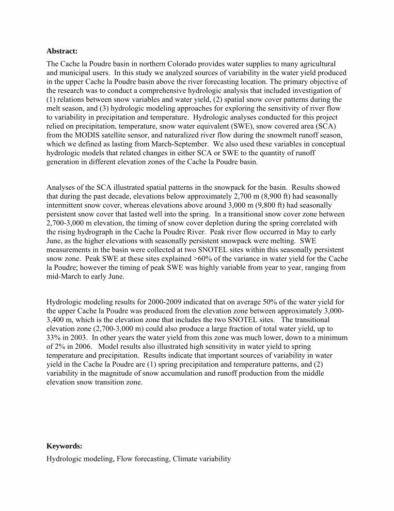
Abstract:
The Cache la Poudre basin in northern Colorado provides water supplies to many agricultural and municipal users. In this study we analyzed sources of variability in the water yield produced in the upper Cache la Poudre basin above the river forecasting location. The primary objective of the research was to conduct a comprehensive hydrologic analysis that included investigation of (1) relations between snow variables and water yield, (2) spatial snow cover patterns during the melt season, and (3) hydrologic modeling approaches for exploring the sensitivity of river flow to variability in precipitation and temperature. Hydrologic analyses conducted for this project relied on precipitation, temperature, snow water equivalent (SWE), snow covered area (SCA) from the MODIS satellite sensor, and naturalized river flow during the snowmelt runoff season, which we defined as lasting from March-September. We also used these variables in conceptual hydrologic models that related changes in either SCA or SWE to the quantity of runoff generation in different elevation zones of the Cache la Poudre basin.
Analyses of the SCA illustrated spatial patterns in the snowpack for the basin. Results showed that during the past decade, elevations below approximately 2,700 m (8,900 ft) had seasonally intermittent snow cover, whereas elevations above around 3,000 m (9,800 ft) had seasonally persistent snow cover that lasted well into the spring. In a transitional snow cover zone between 2,700-3,000 m elevation, the timing of snow cover depletion during the spring correlated with the rising hydrograph in the Cache la Poudre River. Peak river flow occurred in May to early June, as the higher elevations with seasonally persistent snowpack were melting. SWE measurements in the basin were collected at two SNOTEL sites within this seasonally persistent snow zone. Peak SWE at these sites explained >60% of the variance in water yield for the Cache la Poudre; however the timing of peak SWE was highly variable from year to year, ranging from mid-March to early June.
Hydrologic modeling results for 2000-2009 indicated that on average 50% of the water yield for the upper Cache la Poudre was produced from the elevation zone between approximately 3,000-3,400 m, which is the elevation zone that includes the two SNOTEL sites. The transitional elevation zone (2,700-3,000 m) could also produce a large fraction of total water yield, up to 33% in 2003. In other years the water yield from this zone was much lower, down to a minimum of 2% in 2006. Model results also illustrated high sensitivity in water yield to spring temperature and precipitation. Results indicate that important sources of variability in water yield in the Cache la Poudre are (1) spring precipitation and temperature patterns, and (2) variability in the magnitude of snow accumulation and runoff production from the middle elevation snow transition zone.
Keywords:
Hydrologic modeling, Flow forecasting, Climate variability


List of Figures
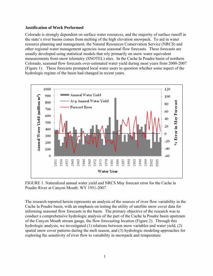
1. Naturalized annual water yield and NRCS May forecast error for the Cache la Poudre River at Canyon Mouth: WY 1951-2007.
2. Location map for the Cache la Poudre basin with SNOTEL, meteorological (COOP) station, and stream gauge measurement locations, including the forecasting location at the Canyon Mouth.
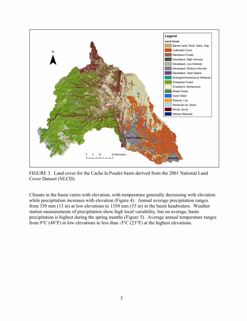
3. Land cover for the Cache la Poudre basin derived from the 2001 National Land Cover Dataset (NLCD).
4. Average annual precipitation for the Cache la Poudre basin derived from the PRISM climate model (www.prismclimate.org). Averages calculated over the years 1971-2000.
5. Average monthly precipitation and temperature for the Cache la Poudre basin, 1971-2000. Derived from PRISM, Oregon State University, www.prismclimate.org.
6. Observed and naturalized discharge (Q) for the Cache la Poudre River at Canyon Mouth, WY 2000.
7. Sub-basins and elevation zones used in analyses of SCA.
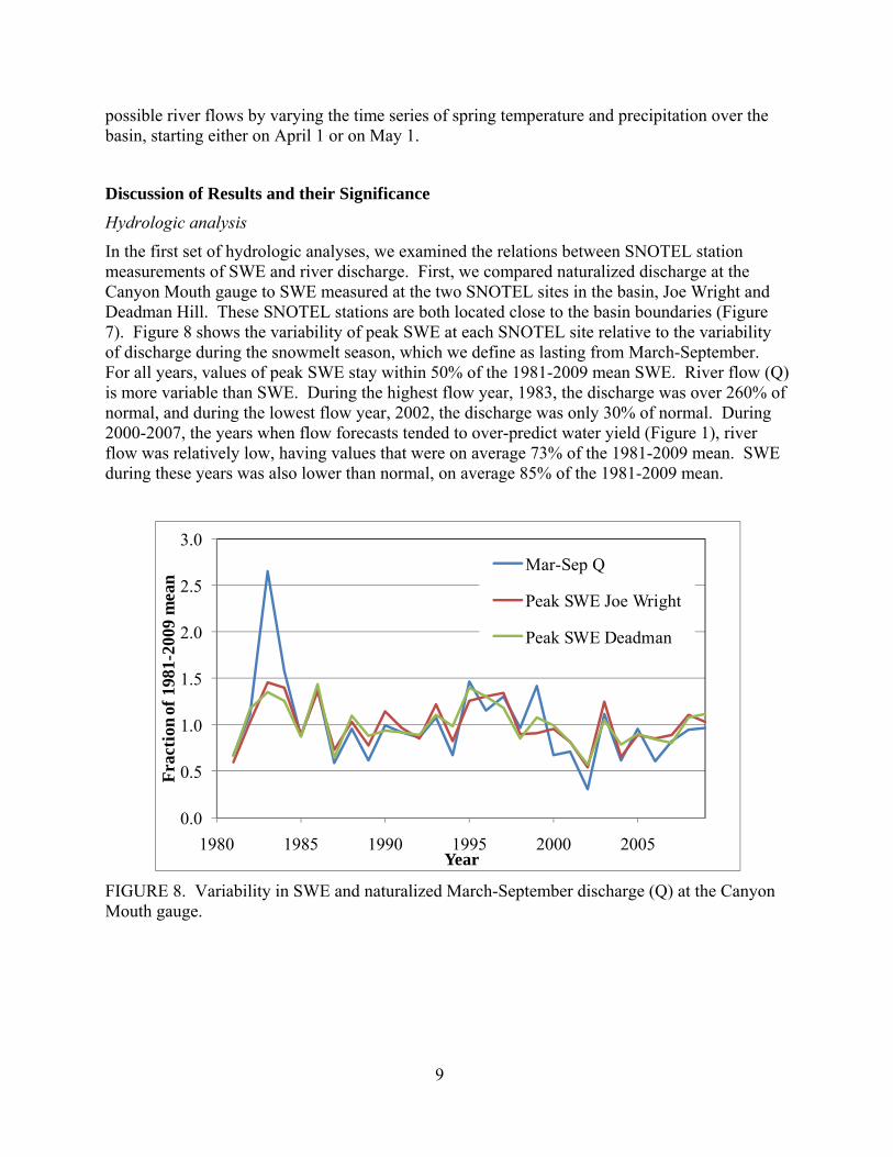
8. Variability in SWE and naturalized March-September discharge (Q) at the Canyon Mouth gauge.
9. March-September naturalized discharge at the Canyon Mouth gauge vs. (a) April 1 SWE, (b) May 1 SWE, and (c) Peak SWE.
10. Variability in (a) SWE at Joe Wright SNOTEL station (elevation 3085 m), (b) %SCA for the basin derived from MODIS, and (c) 7-day mean naturalized discharge at the Canyon Mouth gauge for 2000-2006.
11. Correlation strength (R2) of the SCA vs. Q relationship during the snowmelt seasons for the entire upper Cache la Poudre basin and for sub-basins, 2000-2006.
12. Correlation strength (R2) of the SCA vs. Q relationship during the snowmelt seasons for elevation zones above the Canyon Mouth gauge, 2000-2006.
13. Probability of snow time series for the upper Cache la Poudre basin derived from MODIS 8-day snow covered area images. For each date, probabilities are calculated using images from 2000-2006.
14. Naturalized March-September discharge at Canyon Mouth vs. April 1 SWE (left) and zone 4 SCA (right) during 2000-2009.

15. Observed naturalized discharge and simulated discharge at the Cache la Poudre Canyon
Mouth gauge for 2002 and 2003.
16. Average runoff production by elevation zone for the SCA model and SWE model during 2000-2009. For reference, the plot also shows the fraction of total basin area within each elevation zone.
17. SWE model ensemble simulations illustrating the sensitivity of 2001 discharge to spring precipitation and temperature. (1) Temperature varies in each simulation run starting on April 1; (2) Precipitation varies in each simulation starting on April 1; (3) Temperature varies in each simulation starting on May 1; (4) Precipitation varies in each simulation starting on May 1. For each set of scenarios, varying time series of temperature and precipitation are taken from observed records for 2000 (T0, P0) to 2009 (T9, P9).
18. Box and whisker plot of the bias distribution for each set of hydrograph ensembles in Figure 17. The bias is calculated as the fractional difference between the total flow volume of the simulation and the total flow volume observed in 2001.
List of Tables
1. Meteorological and SNOTEL stations within and near the upper Cache la Poudre basin.
2. Coefficient of determination (R2) between SWE at SNOTEL stations and naturalized March-Sept discharge at the Canyon Mouth Gauge.
3. Coefficient of determination (R2) between SWE at SNOTEL stations, SCA in elevation zone 4 (2680-3042 m), and naturalized March-Sept discharge at the Canyon Mouth Gauge. R2 values are derived from measurements during 2000-2009.
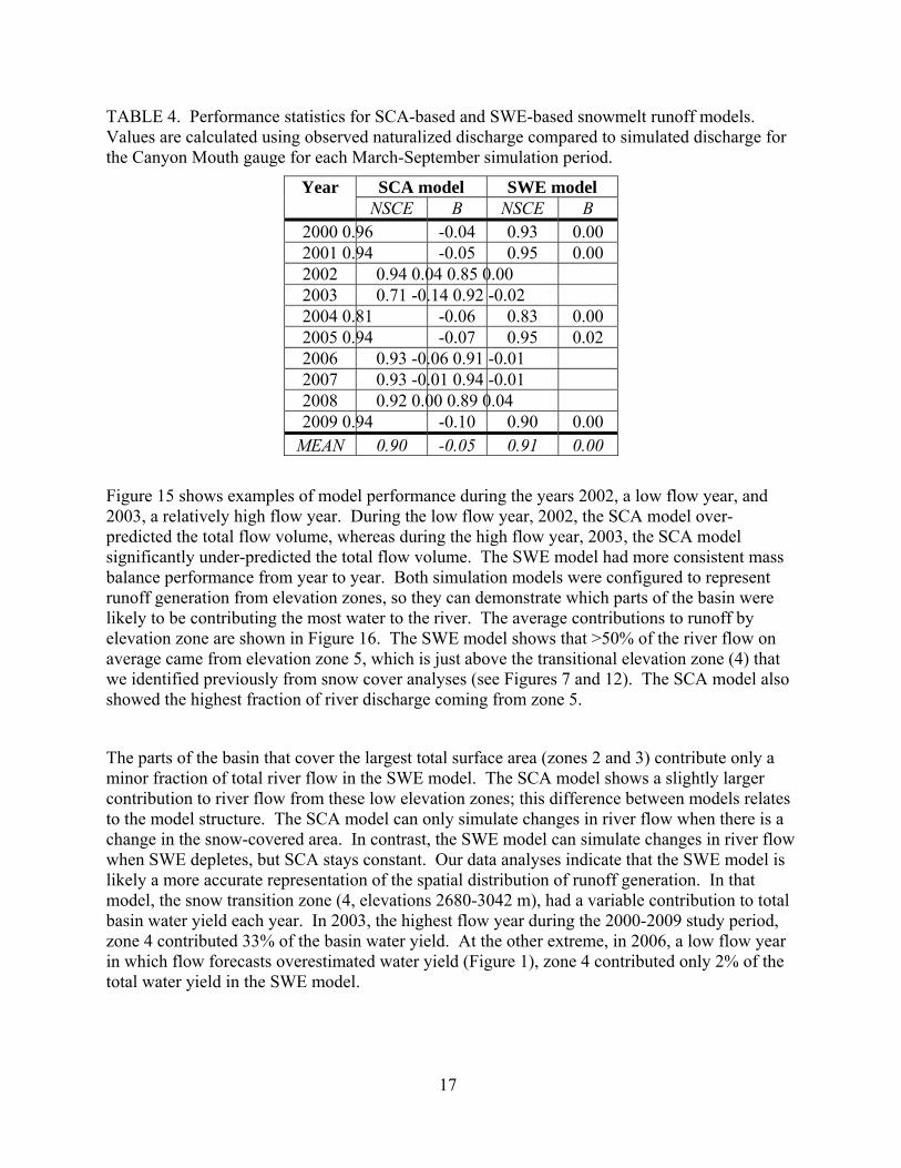
4. Performance statistics for SCA-based and SWE-based snowmelt runoff models. Values are calculated using observed naturalized discharge compared to simulated discharge for the Canyon Mouth gauge for each March-September simulation period.
Justifica
Coloradothe state’resource other regusually dmeasuremColorado(Figure 1hydrolog
FIGUREPoudre R
The reseaCache la informinconduct aof the Cahydrologspatial snexploring
ation of Wor
o is strongly ’s river basinplanning an
gional water developed usments from so, seasonal fl1). These fogic regime of
E 1. NaturalizRiver at Cany
arch reportedPoudre basig seasonal fla comprehenanyon Mouthgic analysis, now cover pag the sensitiv
rk Performe
dependent ons comes frond managememanagemen
sing statisticasnow telemelow forecastorecasts promf the basin ha
zed annual wyon Mouth:
d herein reprin, with an e
flow forecastnsive hydroloh stream gauwe investigaatterns durinvity of river
ed
on surface wom melting oent, the Natu
nt agencies isal models thetry (SNOTEts over-estimmpted local wad changed i
water yield aWY 1951-2
resents an anmphasis on ts in the basiogic analysi
uge, the flowated (1) relatng the melt sflow to vari
1
water resourcof the high elural Resourcssue seasona
hat rely primaEL) sites. Inmated water ywater users tin recent yea
and NRCS M007.
nalysis of thetesting the u
in. The prims of the part
w forecastingtions betweeeason, and (ability in sno
es, and the mlevation snoces Conservaal flow forecarily on snow
n the Cache lyield during to question wars.
May forecast
e sources of utility of satemary objectiv
of the Cachg location (Fien snow vari(3) hydrologowpack and
majority of swpack. To ation Servicecasts. These w water equla Poudre bamost years
whether som
error for the
f river flow vellite snow cve of the resehe la Poudre igure 2). Thiables and w
gic modelingd temperature
surface runofaid in water e (NRCS) anforecasts ar
uivalent asin of northefrom 2000-2
me aspect of t
e Cache la
variability incover data foearch was tobasin upstre
hrough this water yield, (2g approaches e.
ff in
nd re
ern 2007 the
n the or o eam
2) for
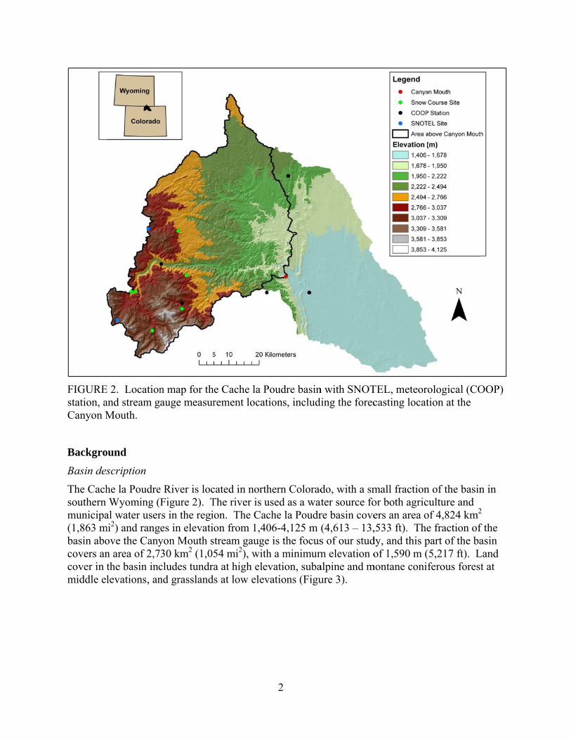
FIGUREstation, aCanyon M
Backgro
Basin des
The Cachsouthern municipa(1,863 mbasin abocovers ancover in tmiddle el
E 2. Locationand stream gMouth.
ound
scription
he la PoudreWyoming (
al water usermi2) and rangove the Canyn area of 2,7the basin inclevations, an
n map for thauge measur
e River is locFigure 2). Trs in the regies in elevatiyon Mouth s30 km2 (1,05cludes tundrand grassland
e Cache la Prement locat
cated in northThe river is uon. The Cacon from 1,40
stream gauge54 mi2), witha at high eles at low elev
2
Poudre basintions, includ
hern Coloradused as a wache la Poudr06-4,125 m e is the focush a minimum
evation, subavations (Figu
n with SNOTding the forec
do, with a smater source fore basin cove(4,613 – 13,s of our studm elevation oalpine and mure 3).
TEL, meteorcasting locat
mall fractionor both agricers an area o,533 ft). Thedy, and this pof 1,590 m (
montane coni
ological (COtion at the
n of the basinculture and of 4,824 km2
e fraction ofpart of the ba(5,217 ft). Lferous forest
OOP)
n in
2 f the asin
Land t at
FIGURECover Da
Climate iwhile prefrom 330station mprecipitatfrom 9°C
E 3. Land coataset (NLCD
in the basin vecipitation in0 mm (13 in)
measurementstion is highe
C (48°F) at lo
over for the CD).
varies with encreases with) at low elevs of precipitaest during theow elevation
Cache la Pou
elevation, wh elevation (ations to 135ation show he spring monns to less tha
3
udre basin de
ith temperat(Figure 4). A50 mm (53 ihigh local vanths (Figure
an -5°C (23°F
erived from
ture generallAnnual averin) in the basariability, bu 5). AveragF) at the hig
the 2001 Na
ly decreasingrage precipitasin headwateut on averagege annual temghest elevatio
ational Land
g with elevatation rangesers. Weathee, basin mperature ranons.
d
tion
er
nges

FIGUREclimate m
FIGURE2000. De
E 4. Averagemodel (www
E 5. Averageerived from
e annual precw.prismclima
e monthly prPRISM, Ore
cipitation forate.org). Ave
recipitation aegon State U
4
r the Cache erages calcu
and temperatUniversity, w
la Poudre baulated over th
ture for the Cwww.prismcl
asin derived he years 197
Cache la Poulimate.org.
from the PR71-2000.
udre basin, 1
RISM
1971-
5
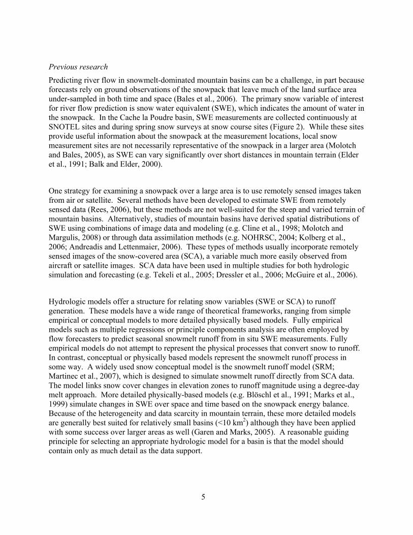
Previous research
Predicting river flow in snowmelt-dominated mountain basins can be a challenge, in part because forecasts rely on ground observations of the snowpack that leave much of the land surface area under-sampled in both time and space (Bales et al., 2006). The primary snow variable of interest for river flow prediction is snow water equivalent (SWE), which indicates the amount of water in the snowpack. In the Cache la Poudre basin, SWE measurements are collected continuously at SNOTEL sites and during spring snow surveys at snow course sites (Figure 2). While these sites provide useful information about the snowpack at the measurement locations, local snow measurement sites are not necessarily representative of the snowpack in a larger area (Molotch and Bales, 2005), as SWE can vary significantly over short distances in mountain terrain (Elder et al., 1991; Balk and Elder, 2000).
One strategy for examining a snowpack over a large area is to use remotely sensed images taken from air or satellite. Several methods have been developed to estimate SWE from remotely sensed data (Rees, 2006), but these methods are not well-suited for the steep and varied terrain of mountain basins. Alternatively, studies of mountain basins have derived spatial distributions of SWE using combinations of image data and modeling (e.g. Cline et al., 1998; Molotch and Margulis, 2008) or through data assimilation methods (e.g. NOHRSC, 2004; Kolberg et al., 2006; Andreadis and Lettenmaier, 2006). These types of methods usually incorporate remotely sensed images of the snow-covered area (SCA), a variable much more easily observed from aircraft or satellite images. SCA data have been used in multiple studies for both hydrologic simulation and forecasting (e.g. Tekeli et al., 2005; Dressler et al., 2006; McGuire et al., 2006).
Hydrologic models offer a structure for relating snow variables (SWE or SCA) to runoff generation. These models have a wide range of theoretical frameworks, ranging from simple empirical or conceptual models to more detailed physically based models. Fully empirical models such as multiple regressions or principle components analysis are often employed by flow forecasters to predict seasonal snowmelt runoff from in situ SWE measurements. Fully empirical models do not attempt to represent the physical processes that convert snow to runoff. In contrast, conceptual or physically based models represent the snowmelt runoff process in some way. A widely used snow conceptual model is the snowmelt runoff model (SRM; Martinec et al., 2007), which is designed to simulate snowmelt runoff directly from SCA data. The model links snow cover changes in elevation zones to runoff magnitude using a degree-day melt approach. More detailed physically-based models (e.g. Blöschl et al., 1991; Marks et al., 1999) simulate changes in SWE over space and time based on the snowpack energy balance. Because of the heterogeneity and data scarcity in mountain terrain, these more detailed models are generally best suited for relatively small basins (<10 km2) although they have been applied with some success over larger areas as well (Garen and Marks, 2005). A reasonable guiding principle for selecting an appropriate hydrologic model for a basin is that the model should contain only as much detail as the data support.

6
Review of Methods Used
Hydrologic analyses conducted for this project rely on precipitation, temperature, snowpack, and river flow measurements during the snowmelt runoff season, which we define as lasting from March-September. We focused most analyses on the years 2000-2009, as these are the years for which we had both SCA data and daily naturalized flow data.
Data sources
We compiled daily precipitation and temperature data for all COOP meteorological stations and SNOTEL stations within and near the boundaries of the upper Cache la Poudre basin (Figure 2, Table 1). We also compiled maps of annual average precipitation and temperature distributions from the PRISM climate model (Figure 4; www.prismclimate.org). To characterize snowpack properties, we compiled daily snow water equivalent (SWE) values for SNOTEL stations and used snow covered area (SCA) images from the Moderate Resolution Imaging Spectroradiometer (MODIS) sensor on the Terra satellite. We used the 8-day maximum SCA product downloaded from the National Snow and Ice Data Center (NSIDC: http://nsidc.org/data/modis/index.html).
TABLE 1. Meteorological and SNOTEL stations within and near the upper Cache la Poudre basin.
Name ID Type Elevation
(m) Fort Collins 53005 COOP 1525 Virginia Dale 58690 COOP 2138 Buckhorn Mountain 51060 COOP 2256 Rustic 57296 COOP 2347 Hourglass 54135 COOP 2902 Joe Wright 05J37S SNOTEL 3085 Deadman Hill 05J06S SNOTEL 3115
To analyze how precipitation, snowpack, and temperature relate to river flow, we require ‘naturalized’ flow values. When the Cache la Poudre River reaches the Canyon Mouth stream gauge, its flow has been modified by diversions into and out of the basin and by reservoir storage. Our analyses use naturalized flow values at the Canyon Mouth location calculated using a basic accounting method:
Naturalized flow = Observed flow + Diversions – Foreign water ± ∆Storage
where Diversions are any structures that remove water from the river or its upstream tributaries, Foreign water is any water that is imported from outside the basin boundaries into the Cache la Poudre or its upstream tributaries, and ∆Storage is any change in the quantity of water stored in reservoirs within the basin. This accounting method does not incorporate routing of flow within the stream network, which contributes some uncertainty to daily naturalized flow values. Calculations of naturalized flow also exclude some smaller diversions that are not monitored
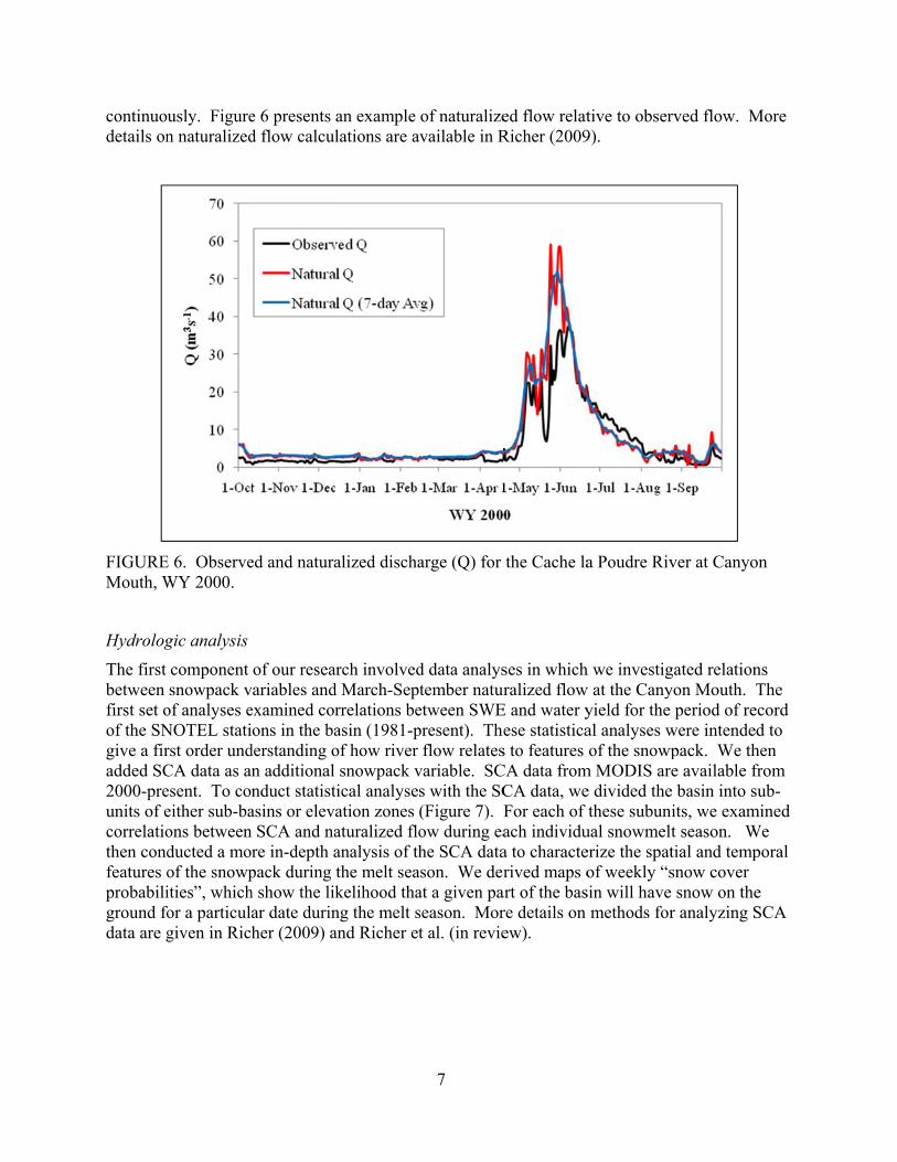
continuoudetails on
FIGUREMouth, W
Hydrolog
The first between first set oof the SNgive a firadded SC2000-preunits of ecorrelatiothen condfeatures oprobabiliground fodata are g
usly. Figuren naturalized
E 6. ObserveWY 2000.
gic analysis
component snowpack v
of analyses eNOTEL statirst order undCA data as anesent. To coneither sub-baons betweenducted a moof the snowpities”, whichor a particulagiven in Rich
e 6 presents d flow calcul
ed and natura
of our reseavariables andexamined corons in the ba
derstanding on additional nduct statist
asins or eleva SCA and nare in-depth apack during h show the likar date durinher (2009) a
an example lations are a
alized discha
arch involvedd March-Seprrelations beasin (1981-pof how river snowpack v
tical analysesation zones aturalized floanalysis of ththe melt seakelihood thang the melt sand Richer et
7
of naturalizevailable in R
arge (Q) for
d data analystember natur
etween SWEpresent). The
flow relatesvariable. SCs with the SC(Figure 7). Fow during eahe SCA data
ason. We derat a given paseason. Mort al. (in revie
ed flow relatRicher (2009
the Cache la
ses in whichuralized flowE and water yese statistica
s to features CA data fromCA data, weFor each of ach individua to characterived maps o
art of the basre details on ew).
tive to obser9).
a Poudre Riv
h we investigw at the Cany
yield for the al analyses wof the snowp
m MODIS aree divided thethese subun
ual snowmelterize the spatof weekly “ssin will have
methods for
rved flow. M
ver at Canyo
gated relationyon Mouth.
period of rewere intendepack. We the available f
e basin into sits, we examt season. Wtial and tempsnow cover snow on ther analyzing S
More
on
ns The
ecord ed to hen from sub-
mined We poral
e SCA

FIGUREused in h
Hydrolog
As a comsimulate SWE, anhydrologstructure simulatesoriginal vusing thecalibrated
We then SWE, ratstudy of tsimulatinKampf anunknown
E 7. Sub-bashydrologic si
gic modeling
mplement to triver flow a
nd SCA. Becgic model, w
of the Snows river flow aversion of SRe elevation zod parameters
developed ather than chathe SCA-dri
ng the observnd Richer (inn spring prec
ins and elevimulation mo
g
the data-bass a function cause the base used a low
wmelt Runofas a functionRM model toones shown s and with st
a new modelanges in SCAiven and SWved river flown preparation
cipitation and
vation zones odels.
ed hydrologof the climasin has a rela
w-parameter ff Model (SRn of changeso simulate flin Figure 7.
tandardized
structure thA as in the o
WE-driven mow in the basn). Using thd temperatur
8
used in anal
gic analyses, ate variables atively limitconceptual m
RM; Martines in SCA in eflow for the s
For each yeparameters,
hat simulates original SRModel structurin. These m
he SWE modre on river fl
lyses of SCA
we develop we analyzed
ted amount omodeling apec et al., 200elevation zonsnowmelt ruear, we ran tas described
river flow aM model. Wres to determ
methods are rdel, we then low predictio
A; elevation
ed conceptud: temperatu
of data to infpproach that 7). The SRMnes. Initially
unoff seasonsthe model wd in Richer (
as a functionWe conducted
mine which ireported in gexplore the on. We creat
zones are al
ual models thure, precipitaform a detailis similar to
M model y, we applies of 2000-20
with both (2009).
n of changes d a comparatis best suitedgreater detaileffects of te ensemble
so
hat ation, led the
ed the 006
in ive
d for l in
s of
9
possible river flows by varying the time series of spring temperature and precipitation over the basin, starting either on April 1 or on May 1.
Discussion of Results and their Significance
Hydrologic analysis
In the first set of hydrologic analyses, we examined the relations between SNOTEL station measurements of SWE and river discharge. First, we compared naturalized discharge at the Canyon Mouth gauge to SWE measured at the two SNOTEL sites in the basin, Joe Wright and Deadman Hill. These SNOTEL stations are both located close to the basin boundaries (Figure 7). Figure 8 shows the variability of peak SWE at each SNOTEL site relative to the variability of discharge during the snowmelt season, which we define as lasting from March-September. For all years, values of peak SWE stay within 50% of the 1981-2009 mean SWE. River flow (Q) is more variable than SWE. During the highest flow year, 1983, the discharge was over 260% of normal, and during the lowest flow year, 2002, the discharge was only 30% of normal. During 2000-2007, the years when flow forecasts tended to over-predict water yield (Figure 1), river flow was relatively low, having values that were on average 73% of the 1981-2009 mean. SWE during these years was also lower than normal, on average 85% of the 1981-2009 mean.
FIGURE 8. Variability in SWE and naturalized March-September discharge (Q) at the Canyon Mouth gauge.
0.0
0.5
1.0
1.5
2.0
2.5
3.0
1980 1985 1990 1995 2000 2005
Fra
ctio
n of
198
1-20
09 m
ean
Year
Mar-Sep Q
Peak SWE Joe Wright
Peak SWE Deadman
10
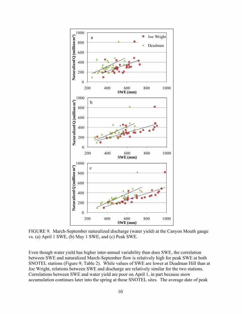
FIGURE 9. March-September naturalized discharge (water yield) at the Canyon Mouth gauge vs. (a) April 1 SWE, (b) May 1 SWE, and (c) Peak SWE.
Even though water yield has higher inter-annual variability than does SWE, the correlation between SWE and naturalized March-September flow is relatively high for peak SWE at both SNOTEL stations (Figure 9; Table 2). While values of SWE are lower at Deadman Hill than at Joe Wright, relations between SWE and discharge are relatively similar for the two stations. Correlations between SWE and water yield are poor on April 1, in part because snow accumulation continues later into the spring at these SNOTEL sites. The average date of peak
0
200
400
600
800
1000
200 400 600 800 1000
Nat
ural
ized
Q (m
illi
on m
3 )
SWE (mm)
Joe Wright
Deadman
0
200
400
600
800
1000
200 400 600 800 1000
Nat
ural
ized
Q (m
illi
on m
3 )
SWE (mm)
0
200
400
600
800
1000
200 400 600 800 1000
Nat
ural
ized
Q (m
illi
on m
3 )
SWE (mm)
a
b
c
11
SWE is May 2 at Joe Wright and May 4 at Deadman Hill. As a result, correlations between SWE and water yield improve substantially for May 1. However, the date of peak SWE at the two stations can vary from mid-March to early June, meaning that May 1 is not always an ideal date for water yield prediction. The SWE variable that has the highest correlation to March-September discharge is the peak SWE, which explains >60% of variance in discharge. If the outlying high flow year (1983) is excluded, the peak SWE explains >70% of variance in discharge (Table 2).
TABLE 2. Coefficient of determination (R2) between SWE at SNOTEL stations and naturalized March-Sept discharge at the Canyon Mouth Gauge.
Joe Wright Deadman Apr 1, all data 0.29 0.30 Apr 1, excluding 1983 0.28 0.27 May 1, all data 0.50 0.46 May 1, excluding 1983 0.57 0.53 Peak, all data 0.64 0.61 Peak, excluding 1983 0.72 0.73
The two SNOTEL stations are both located at the margins of the basin, Joe Wright at 3085 m elevation and Deadman at 3115 m elevation. An additional SNOTEL station was added at the Hourglass site (2902 m elevation) in 2008, but before then, there were no continuous measurements of SWE at lower elevations within the basin. The MODIS SCA data allow us to examine snow behavior in parts of the basin where in situ measurements are unavailable. Figure 10 shows examples of how SWE at Joe Wright and SCA for the basin as a whole compare to naturalized discharge during snowmelt. During many of the years shown, SWE at Joe Wright continued to accumulate until May. In contrast, SCA for the basin as a whole began to decrease in mid-March each year, well before the high elevation snowpack at Joe Wright had begun to melt. Discharge in the river generally stayed at baseflow levels until mid-April, when it began to rise gradually. River flow rose to peak flow levels in mid-May to early June, when the high elevation snowpack was melting.
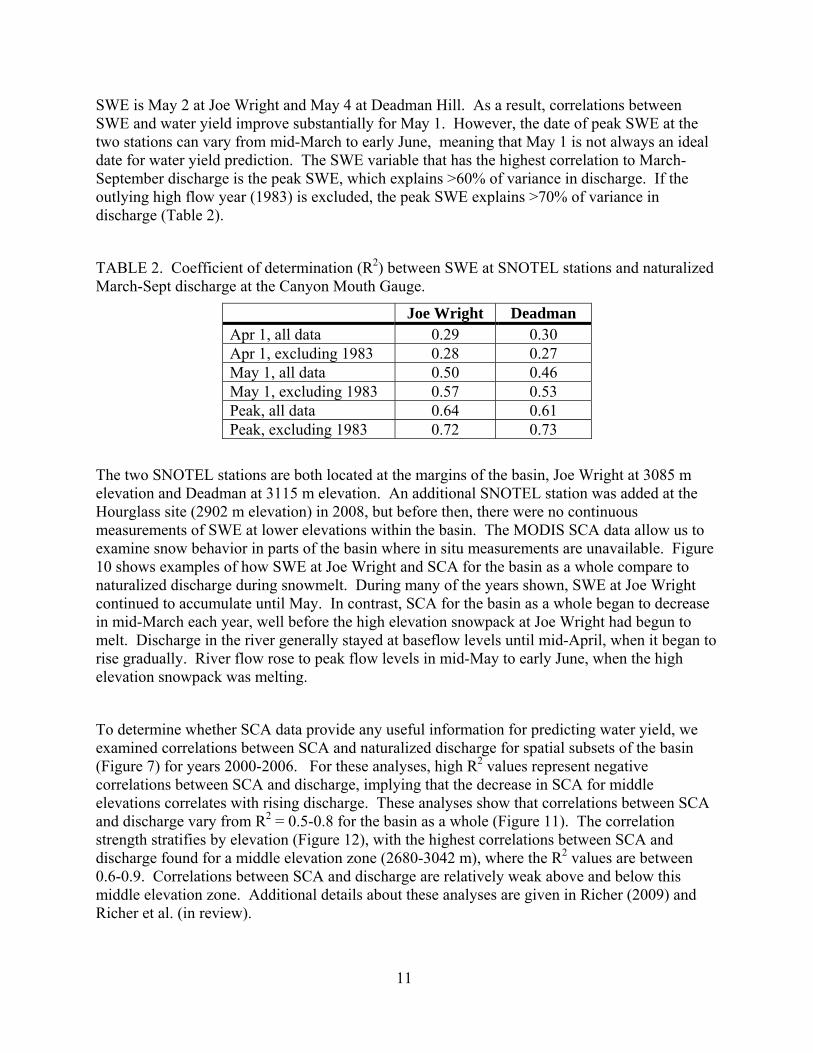
To determine whether SCA data provide any useful information for predicting water yield, we examined correlations between SCA and naturalized discharge for spatial subsets of the basin (Figure 7) for years 2000-2006. For these analyses, high R2 values represent negative correlations between SCA and discharge, implying that the decrease in SCA for middle elevations correlates with rising discharge. These analyses show that correlations between SCA and discharge vary from R2 = 0.5-0.8 for the basin as a whole (Figure 11). The correlation strength stratifies by elevation (Figure 12), with the highest correlations between SCA and discharge found for a middle elevation zone (2680-3042 m), where the R2 values are between 0.6-0.9. Correlations between SCA and discharge are relatively weak above and below this middle elevation zone. Additional details about these analyses are given in Richer (2009) and Richer et al. (in review).

FIGURE%SCA foCanyon M
E 10. Variabor the basin Mouth gauge
ility in (a) Sderived frome for 2000-2
SWE at Joe Wm MODIS, a2006.
12
Wright SNOTand (c) 7-day
TEL station y mean natur
(elevation 3ralized disch
3085 m), (b)harge at the
FIGUREseasons f
FIGUREseasons f
E 11. Correlafor the entire
E 12. Correlafor elevation
ation strengte upper Cach
ation strengtn zones abov
th (R2) of thehe la Poudre
th (R2) of theve the Canyo
13
e SCA vs. Qbasin and fo
e SCA vs. Qon Mouth gau
Q relationshipor sub-basin
Q relationshipuge, 2000-20
p during the ns, 2000-200
p during the 006.
snowmelt 6.
snowmelt

FIGUREMODIS images fr
E 13. Probab8-day snow rom 2000-20
bility of snowcovered area
006.
w time seriesa images. F
14
s for the uppor each date
per Cache la e, probabiliti
Poudre basies are calcul
in derived frolated using
om
15
To explore the spatial patterns of SCA in greater detail, we developed composite images that demonstrate the likelihood of snow cover for each pixel in the basin during the snowmelt season (Figure 13). As shown in Figure 13, the “Probability of Snow” for each pixel is calculated as the number of images with snow cover on the specified date divided by the total number of images in the period of analysis. Values of 1 indicate that all images on the specified date were snow-covered; values of 0 indicate that no images on the specified date were snow-covered. The probability of snow cover for the basin shows a gradual change with elevation during late March and early April. By mid-late April, however, the probability of snow images develop a sharp transition between low snow cover and high snow cover. This sharp transition zone develops just below approximately 3000 m elevation, in the range of the middle elevation zone (4) highlighted in Figure 12. The snow cover is intermittent below this transition zone, whereas snow cover persists well into the spring above the transition zone.
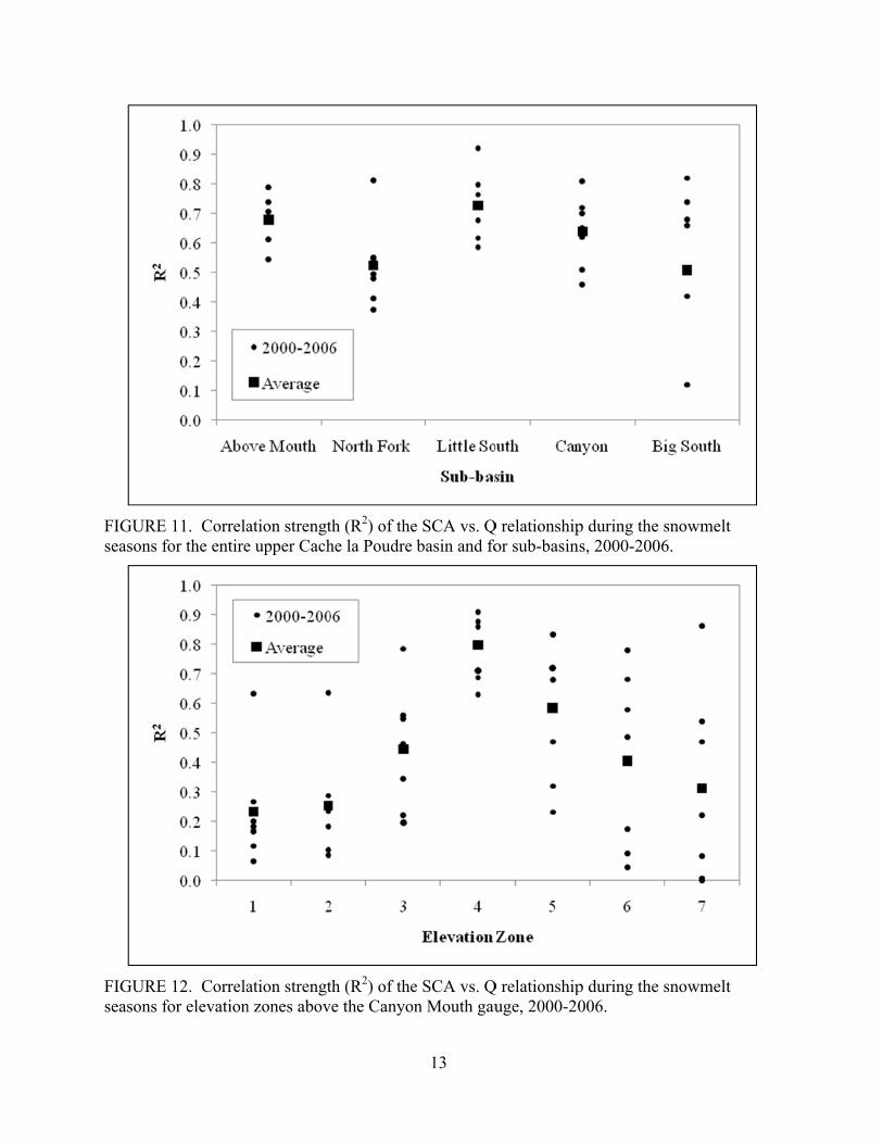
Our snow cover analyses showed that the snowed cover transition zone is a prominent feature of the basin snowpack. Snow cover changes only correlated consistently with runoff timing within this mid-elevation transition zone (Figure 12), which is located below the elevations of SNOTEL measurements of SWE. Information about the spatial extent of the seasonal snowpack in these lower elevations could potentially be helpful in predicting early season runoff. Our initial analyses comparing SCA in the transitional elevation zone to river flow during 2000-2006 suggested that SCA in early April could be a strong predictor of March-September water yield. However, subsequent analyses including additional years of data showed mixed results. Figure 14 and Table 3 compare predictions of March-September discharge using either April 1 SWE or SCA from March 29 or April 6 in the snow transition zone (4). The SCA dates correspond to the dates when 8-day maximum SCA images from MODIS were available. Of the variables tested in Figure 14, SCA on April 6 had the strongest correlation to water yield, but its R2 value was still only 0.59.
FIGURE 14. Naturalized March-September discharge at Canyon Mouth vs. April 1 SWE (left) and zone 4 SCA (right) during 2000-2009.
0
200
400
200 400 600 800 1000
Nat
ural
ized
Q (m
illi
on m
3 )
SWE (mm)
Joe Wright
Deadman
0
200
400
40 60 80 100
Nat
ural
ized
Q (m
illi
on m
3 )
SCA (%)
Mar 29 SCAApr 6 SCA

16
TABLE 3. Coefficient of determination (R2) between snow variables (SWE at SNOTEL stations or SCA in elevation zone 4) and naturalized March-Sept discharge at the Canyon Mouth Gauge. R2 values are derived from measurements during 2000-2009.
R2 Apr 1 SWE, Joe Wright 0.53 Apr 1 SWE, Deadman 0.44 Mar 29 SCA, zone 4 0.41 Apr 6 SCA, zone 4 0.59
After the first week of April, SWE always out-performed SCA as a predictor variable for water yield. In part this is because SCA only has potential benefit as a runoff predictor variable in areas like the snow transition zone, where snow cover depletion correlates with a river flow response. SCA has limited utility in representing runoff under conditions when snow is melting from an area that remains entirely snow covered. During 2007-2009, for example, SCA in the transitional elevation zone was at or near 100% on March 29 and April 6 (Figure 14), making it impossible to use SCA to distinguish between flow volumes for these years. Additional years of data are likely needed to determine whether and how SCA data can be a useful quantitative addition to statistical flow forecasts. Qualitatively, however, the SCA data do demonstrate how rapidly snow cover depletes from the basin and where the snowpack is seasonally persistent. Both of these types of information are useful for determining how much of the basin area is likely to contribute to river water yield.
Hydrologic modeling
Hydrologic simulation models enable us to explore mechanistic relationships between the snow variables we analyzed (SWE and SCA) and river flow. We developed two separate simulation models, one driven by changes in SWE and the other driven by changes in SCA. These models simulate discharge at the Canyon Mouth gauging location at a daily time step during March-September for 2000-2009, the years when SCA data were available for the basin. Models both have strong performance (Table 4), with average Nash-Sutcliffe Efficiency Coefficients (NSCE) of 0.90 for the SCA model and 0.91 for the SWE model. Mass balance performance is described by the Bias statistic (B), which indicates the fractional difference between measured and simulated total March-September discharge. The SWE model has a low mass balance error on average, whereas the SCA model tends to under-predict total discharge. Additional details on hydrologic model calibration and performance are given in Kampf and Richer (in preparation).
17
TABLE 4. Performance statistics for SCA-based and SWE-based snowmelt runoff models. Values are calculated using observed naturalized discharge compared to simulated discharge for the Canyon Mouth gauge for each March-September simulation period.
Year SCA model SWE model NSCE B NSCE B
2000 0.96 -0.04 0.93 0.00 2001 0.94 -0.05 0.95 0.00 2002 0.94 0.04 0.85 0.00 2003 0.71 -0.14 0.92 -0.02 2004 0.81 -0.06 0.83 0.00 2005 0.94 -0.07 0.95 0.02 2006 0.93 -0.06 0.91 -0.01 2007 0.93 -0.01 0.94 -0.01 2008 0.92 0.00 0.89 0.04 2009 0.94 -0.10 0.90 0.00
MEAN 0.90 -0.05 0.91 0.00
Figure 15 shows examples of model performance during the years 2002, a low flow year, and 2003, a relatively high flow year. During the low flow year, 2002, the SCA model over-predicted the total flow volume, whereas during the high flow year, 2003, the SCA model significantly under-predicted the total flow volume. The SWE model had more consistent mass balance performance from year to year. Both simulation models were configured to represent runoff generation from elevation zones, so they can demonstrate which parts of the basin were likely to be contributing the most water to the river. The average contributions to runoff by elevation zone are shown in Figure 16. The SWE model shows that >50% of the river flow on average came from elevation zone 5, which is just above the transitional elevation zone (4) that we identified previously from snow cover analyses (see Figures 7 and 12). The SCA model also showed the highest fraction of river discharge coming from zone 5.
The parts of the basin that cover the largest total surface area (zones 2 and 3) contribute only a minor fraction of total river flow in the SWE model. The SCA model shows a slightly larger contribution to river flow from these low elevation zones; this difference between models relates to the model structure. The SCA model can only simulate changes in river flow when there is a change in the snow-covered area. In contrast, the SWE model can simulate changes in river flow when SWE depletes, but SCA stays constant. Our data analyses indicate that the SWE model is likely a more accurate representation of the spatial distribution of runoff generation. In that model, the snow transition zone (4, elevations 2680-3042 m), had a variable contribution to total basin water yield each year. In 2003, the highest flow year during the 2000-2009 study period, zone 4 contributed 33% of the basin water yield. At the other extreme, in 2006, a low flow year in which flow forecasts overestimated water yield (Figure 1), zone 4 contributed only 2% of the total water yield in the SWE model.

18
FIGURE 15. Observed naturalized discharge and simulated discharge at the Cache la Poudre Canyon Mouth gauge for 2002 and 2003.
FIGURE 16. Average runoff production by elevation zone for the SCA model and SWE model during 2000-2009. For reference, the plot also shows the fraction of total basin area within each elevation zone.
80 100 120 140 160 180 200 220 2400
5
10
15
20
25
30
35
40
Day of Year
Dis
cha
rge
(cm
s)
ObservedSCA modelSWE model
80 100 120 140 160 180 200 220 2400
20
40
60
80
100
120
140
Day of Year
Dis
cha
rge
(cm
s)
ObservedSCA modelSWE model
1 2 3 4 5 6 70
0.1
0.2
0.3
0.4
0.5
0.6
Elevation Zone
Fra
ctio
n o
f tot
al d
isch
arg
e/a
rea
SCA modelSWE modelBasin area
2002
2003

19
After developing and testing the SWE model, we used this model to examine the sensitivity of river flow to spring precipitation and temperature. Because this basin receives high spring precipitation (Figure 5) and often does not experience peak SWE until after May 1, the behavior of the weather in the spring months could have a significant effect on the ability to forecast seasonal river flow. Here we illustrate an example sensitivity analysis for the year 2001. In this example, we assume that the SWE on March 1 is represented by an average lapse function that assigns low SWE to low elevation and higher SWE to high elevations. Each simulation run proceeds at a daily time step starting with this same March 1 SWE distribution and the input precipitation and temperature values from 2001 climate data. Test scenarios then assume (1) temperature is unknown for April 1 to September 30, (2) precipitation is unknown for April 1 to September 30, (3) temperature is unknown for May 1 to September 30, and (4) precipitation is unknown for May 1 to September 30. Each test scenario is run ten times, with the ten ensemble runs taken from the observed temperature or precipitation record for 2000-2009.
FIGURE 17. SWE model ensemble simulations illustrating the sensitivity of 2001 discharge to spring precipitation and temperature. (1) Temperature varies in each simulation run starting on April 1; (2) Precipitation varies in each simulation starting on April 1; (3) Temperature varies in each simulation starting on May 1; (4) Precipitation varies in each simulation starting on May 1. For each set of scenarios, varying time series of temperature and precipitation are taken from observed records for 2000 (T0, P0) to 2009 (T9, P9).
100 150 200 250
10
20
30
40
50
60
70
80
Day of Year
Dis
cha
rge
(cm
s)
ObservedT0T1T2T3T4T5T6T7T8T9
100 150 200 250
10
20
30
40
50
60
70
80
Day of Year
Dis
cha
rge
(cm
s)
ObservedP0P1P2P3P4P5P6P7P8P9
100 150 200 250
10
20
30
40
50
60
70
80
Day of Year
Dis
cha
rge
(cm
s)
ObservedT0T1T2T3T4T5T6T7T8T9
100 150 200 250
10
20
30
40
50
60
70
80
Day of Year
Dis
cha
rge
(cm
s)
ObservedP0P1P2P3P4P5P6P7P8P9
1: T unknown
Apr1-Sep30
2: P unknown
Apr1-Sep30
3: T unknown
May1-Sep30 4: P unknown
May1-Sep30

20
Figure 17 illustrates the results of these ensemble simulation tests. The first two scenarios are intended to represent river flow prediction starting on April 1. Scenario 1 assumes that precipitation is known, but temperature is unknown from April 1 – September 30. Varying the temperature in each of the ensemble runs creates a wide range of simulated hydrographs, which lead to total simulated flow volumes that range from 26% higher than observations to 24% lower than observed flow (Figure 18). Where the precipitation is unknown, but temperature is known (Scenario 2), the range of simulated hydrographs is slightly smaller, from 11% higher than observed flow to 31% lower than observations (Figure 18). Scenarios 1 and 2 demonstrate that without prior knowledge of precipitation and temperature for the melt season, it is difficult to predict accurate hydrographs. Ensemble scenarios are less variable where precipitation and temperature are unknown starting later in the spring (May 1 in Scenarios 3 and 4). For the May 1 scenarios, variable temperature creates a wider range of simulated hydrographs than variable precipitation (Figures 17, 18).
FIGURE 18. Box and whisker plot of the bias distribution for each set of hydrograph ensembles in Figure 17. The bias is calculated as the fractional difference between the total flow volume of the simulation and the total flow volume observed in 2001.
These model sensitivity tests highlight the importance of spring temperature in determining the magnitude and timing of river flow. In the model, temperature during the spring controls both the melting of the snowpack and whether spring precipitation falls as rain or as snow in different elevation zones. Temperature patterns that favor snow accumulation can end up resulting in more simulated runoff because runoff coefficients are higher in the model for snowmelt than they are for rainfall. Sensitivity to temperature in the simulations is also a result of the model structure for simulating the fraction of melt water that reaches the river. Early in the spring, the model assumes that most of the melt water infiltrates and is not available for runoff, whereas later in the melt season, the ground becomes saturated, and more of the melt water reaches the
-0.3
-0.2
-0.1
0
0.1
0.2
1 2 3 4Ensemble Scenario
Bia
s
21
river. Additional research could explore alternate model structures to examine whether different models predict similar sensitivities to spring temperature and precipitation.
Principle Findings, Conclusions, and Recommendations
Hydrologic analyses and modeling results from this study highlight several key features of the snowpack and runoff production in the upper Cache la Poudre basin:
1. Snow cover analyses show seasonally persistent snowpack above around 3,000 m (9,800 ft) elevation that lasts through the winter and early spring.. The snow cover is intermittent below around 2,700 m (8,900 ft) elevation.
2. Modeling results indicate that on average 50% of the total basin water yield comes from the elevation zone between about 3,000-3,400 m (SWE model, Figure 16).
3. The transitional elevation zone identified from snow cover analyses (2,700-3,000 m) has a variable contribution to runoff; in the highest flow year of our study period, 2003, model results indicated that this zone produced 33% of the total water yield, whereas in a lower flow year, 2006, this zone produced only 2% of the total water yield.
4. The timing of snow cover depletion in the transitional elevation zone correlates with the timing of the rising hydrograph, but peak runoff typically does not occur until the higher elevation snowpack begins to melt.
Our results also demonstrate several challenges in spring predictions of water yield in the Cache la Poudre:
1. April and May are the months with the highest average precipitation in the basin (Figure 5). Forecasting is difficult without a priori knowledge of the spring precipitation.
2. Peak snow water equivalent at the two high elevation sites has occurred as early as March 18 (2002 at Joe Wright) and as late as June 2 (1995 at Joe Wright). This variability in the timing of spring snow accumulation means that it is difficult to predict water yield on fixed dates. While peak snow water equivalent explains >60% of variance in water yield from 1981-2009, April 1 SWE and May 1 SWE predict only 30 and 50% of variance in water yield, respectively (Table 2).
3. March-September water yield in the Cache la Poudre River at the Canyon Mouth has greater variability than peak snow water equivalent at the two high elevation SNOTEL sites, Deadman Hill and Joe Wright (Figure 8). Our modeling results suggest two possible causes for variability in water yield that is inconsistent with variability in peak SWE:
a. The elevation zone with transitional snowpack (2700-3000 m) contributes a variable fraction of total water yield, meaning that in some years a high quantity of runoff is produced in this zone, whereas in other years the runoff production in

22
this zone is low. Additional measurements of SWE in these transitional elevations, for example the new SNOTEL site installed at Hourglass, should be helpful for water yield prediction.
b. The timing of spring warming may also affect the quantity of snow that becomes runoff. Model sensitivity tests show that even when spring precipitation is known, differences in spring temperature patterns can produce differences in water yield (Figures 17, 18).
Because we only examined existing measurements of hydrologic variables in this study, our results do not demonstrate the importance of other factors such as dust on snow, sublimation, soil moisture, or groundwater recharge on river discharge. Given the variables we analyzed, we conclude that the challenges in forecasting water yield in the Cache la Poudre relate primarily to (1) high variability in spring precipitation and temperature patterns, which cause the timing of peak snow accumulation to vary from mid-March to early June, and (2) high variability in the quantity of runoff production from the transitional 2,700-3,000 m (8,900-9,800 ft) elevation zone. Future work could incorporate additional hydrologic processes into simulation models and test the sensitivity of water yield to other factors not tested in this study.
23
References
Andreadis, K.M. and D.P. Lettenmaier. 2006. Assimilating remotely sensed snow observations into a macroscale hydrology model. Advances in Water Resources 29: 872-886.
Bales, R.C., N.P. Molotch, T.H. Painter, M.D. Dettinger, R. Rice, J. Dozier, 2006. Mountain hydrology of the western United States. Water Resources Research 42, W08432, doi:10.1029/2005WR004387.
Balk, B., K. Elder, 2000. Combining binary decision tree and geostatistical methods to estimate snow distribution in a mountain watershed. Water Resources Research 36(1), 13-26.
Blöschl, G., R. Kirnbauer, D. Gutknecht, 1991. Distributed snowmelt simulations in an alpine catchment, 1. Model evaluation on the basis of snow cover patterns. Water Resources Research 27(12), 3171-3179.
Cline, D., K. Elder, R. Bales, 1998. Scale effects in a distributed snow water equivalence and snowmelt model for mountain basins. Hydrological Processes 12, 1527-1536.
Dressler, K.A., G.H. Leavesley, R.C. Bales, and S.R. Fassnacht. 2006. Evaluation of gridded snow water equivalent and satellite snow cover products for mountain basins in a hydrologic model. Hydrological Processes 20: 673-688.
Elder, K., J. Dozier, J. Michaelsen, 1991. Snow accumulation and distribution in an alpine watershed. Water Resources Research 27(7), 1541-1552.
Garen, D.C., D. Marks, 2005. Spatially distributed energy balance snowmelt modelling in a mountainous river basin: estimation of meteorological inputs and verification of model results. Journal of Hydrology 315, 126-153.
Kampf, SK, Richer, E.E. (in preparation). Estimating source regions for snowmelt runoff in a Rocky Mountain watershed: comparison of conceptual runoff models driven by snow cover or snow water equivalent.
Kolberg, S., H. Rue, L. Gottschalk, 2006. A Bayesian spatial assimilation scheme for snow coverage observations in a gridded snow model. Hydrology and Earth System Sciences 10, 369-381.
Marks, D., J. Domingo, D. Susong, T. Link, D. Garen, 1999. A spatially distributed energy balance snowmelt model for application in mountain basins. Hydrological Processes 13, 1935-1959.
Martinec, J., A. Rango, and R. Roberts. 2007. Snowmelt Runoff Model User’s Manual, Updated Edition 2007, WinSRM Version 1.11. USDA Jornada Experimental Range, New Mexico State University, Las Cruces, NM 88003, U.S.A.
McGuire, M., A.W. Wood, A.F. Hamlet, D.P. Lettenmaier. 2006. Use of satellite data for streamflow and reservoir storage forecasts in the Snake River basin, Journal of Water Resources Planning and Management 132(2): 97-110.
Molotch, N.P., R.C. Bales, 2005. Scaling snow observations from the point to the grid element: implications for observation network design. Water Resources Research 41, W11421, doi:10.1029/2005WR004229.
Molotch, N.P., and S.A. Margulis. 2008. Estimating the distribution of snow water equivalent using remotely sensed snow cover data and a spatially distributed snowmelt model: A multi-resolution, multi-sensor comparison. Advances in Water Resources 31: 1503-1514.
National Operational Hydrologic Remote Sensing Center. 2004. Snow Data Assimilation System (SNODAS) Data Products at NSIDC. Boulder, Colorado USA: National Snow and Ice Data Center. Digital media.

24
Richer, E.E., 2009. Snowmelt runoff analysis and modeling for the Upper Cache la Poudre River Basin, Colorado. M.S. Thesis, Colorado State University, 117 pp.
Richer, E., Kampf, S., Fassnacht, S. (in review). Relationships between snow cover depletion patterns and snowmelt runoff in a Colorado Front Range watershed.
Tekeli, A.E., Z. Akyurek, A.A. Sorman, A. Sensoy, and A.U. Sorman. 2005. Using MODIS snow cover maps in modeling snowmelt runoff process in the eastern part of Turkey. Remote Sensing of Environment 97: 216-230.