hydrologic modeling for the watersheds 2000 project · appendix a memorandum from seth jelen, pe,...
TRANSCRIPT

Hydrologic Modeling for the Watersheds 2000 Project
Prepared by:
In conjunction with:
October 31, 2001
Revised November 22, 2002 Revised June 2, 2003


TABLE OF CONTENTS Page Introduction 1 Purpose 2 HEC-HMS 2 Meteorological Model 2 Basin Model 5 Control Specifications 18 Results 18 Tables Table 1 Total Rainfall Depths Used for Watersheds 2000 and Flood Insurance
Restudy Hydrology 3 Table 2 Stream Codes and Names 6 Table 3 GIS Zoning Coverage and Percent Impervious Per Category 11 Table 4 ‘N’ Values for Urban Streams 14 Table 5 ‘N’ Values for Large Rivers 15 Figures Figure 1 Study Area Boundaries Figure 2 Tualatin River Subbasins Figure 3 HMS Schematic for Nyberg Creek Model Figure 4 Calibration–20 February 1994–Upper Fanno Creek Figure 5 Calibration-20 February 1994-Lower Fanno Creek Figure 6 Calibration-15 February 1995-Upper Fanno Creek Figure 7 Calibration-15 February 1995-Lower Fanno Creek

Table of Contents (continued)
Figure 8 Calibraton-09 December 1995-Upper Fanno Creek Figure 9 Calibration-09 December 1995-Lower Fanno Creek Figure 10 Calibration-03 February 1996-Upper Fanno Creek Figure 11 Calibration-03 February 1996-Lower Fanno Creek Appendices Appendix A Memorandum from Seth Jelen, PE, PWR to Kendra Smith, CWS, April 2, 2002, PWR Recommends 24-Hour SCS1A Storm for Floodplain Remapping Appendix B MGS Engineering Consultants, Inc., July 9, 2001, Development of Design Storms for the Portland, Oregon Area Appendix C Memorandum from Stephen Blanton, PE, PWR to Kendra Smith, CWS, March 26, 2002, Tualatin River Tributaries Peak Flows
Appendix D Roger C. Sutherland, PE, Methodology for Estimating Lag Time of Natural, Partially Urbanized and Urban Watershed Based on Published U.S.G.S. Data for Watersheds Throughout the Metropolitan Areas of Portland and Salem, Oregon
Appendix E MGS Engineering Consultants, Inc., July 9, 2001, Applications of the Soil Moisture
Accounting Method in the HEC-HMS Model for the Watersheds 2000 Project Appendix F Kurahashi & Associates, Inc., 1997, Appendix A: Fanno Creek Hydrologic
and Hydraulic Analysis, page 10 Appendix G Comparison of Peak Flood Discharges for East, South and Central County

Hydrologic Modeling for the Watersheds 2000 Project
October 31, 2001
Revised November 22, 2002 Revised June 2, 2003
INTRODUCTION Watersheds 2000 is one aspect of the Healthy Streams Plan begun by Clean Water Services (CWS) in October 1999. The Healthy Streams Plan will develop watershed based strategies and master plans which integrate the requirements of both the Clean Water (CWA) and Endangered Species (ESA) Acts. The plan will identify and prioritize policies, programmatic changes and specific projects needed to improve water quality, manage flooding and floodplains and provide for aquatic species recovery in the Tualatin River Basin. Watersheds 2000 provides an inventory of consistent hydrology and hydraulic models to use as a basis for evaluating progress. Due to the scale of the undertaking, CWS contracted with three separate consulting firms to prepare the models. The basin was also subdivided into three regions, one for each of the consultants. (See Figure 1 – Study Area Boundaries.) Pacific Water Resources, Inc. (PWR) was the lead consultant and responsible for developing hydrologic and hydraulic models for the East Region. As lead consultant, PWR organized and led the standardization meetings to coordinate methodology, parameter selection, model schematization and other aspects for all consultants. Using the initial products from Watersheds 2000, PWR also developed the revised hydrology and hydraulics package for the Flood Insurance Restudy (FIR) submittal to FEMA. Philip Williams and Associates, Ltd. (PWA) prepared the hydrologic and hydraulic models for the south region. Tetra Tech, Inc. performed similar services for the central region. MGS Engineering Consultants (MGS), under contract with PWA, prepared HSPF models to assist in parameter selection and model calibration. They also developed two new storm distributions based on statistical analysis of Pacific Northwest rainfall gauges. The complete inventory includes: hydraulic models for over 30 miles of the main stem Tualatin River; flow estimates for the entire Tualatin River valley; existing, future and historic conditions hydrology models of over 460 square miles of tributary watersheds; approximately 169 miles of stream hydraulic models; and a flood insurance restudy for 175 stream miles. Detailed reports are available from CWS for

Hydrologic Modeling for the Watersheds 2000 Project Page 2 Revised June 2, 2003
the hydrology of the Tualatin River as well as historic and future flows for all the tributaries studied. This summary report, prepared by PWR with input from each of the other consultants, presents the basis for the existing and future conditions hydrologic models. These models are used for both the Watersheds 2000 inventory and the FIR submittal. PURPOSE The Clean Water Services' Watersheds 2000 project analyzed the watershed-scale hydrology of 27 drainages in Washington County, all tributaries of the Tualatin River. This technical memorandum, along with the attached reports from MGS and PWR, details the methodology used in developing the hydrologic models of these watersheds. The watersheds within the study area are: Ash, Beaverton, Bronson, Butternut, Cedar Mill, Cedar, Chicken, Council, Cross, Dairy, Dawson, Fanno, Gales, Glencoe, Gordon, Hedges, Johnson South, McKay, Nyberg, Rock, Saum, South Rock, Storey, Summer, Thatcher, Waible, and Willow (See Figure 2 – Tualatin Sub-Watersheds.). The hydrologic models were created using the Hydrologic Engineering Center-Hydrologic Modeling System (HEC-HMS). Modeling was based on winter precipitation events.
HEC-HMS The watershed-scale hydrologic analysis for each of the study areas was accomplished using HEC-HMS. HEC-HMS is a computational modeling system developed by the Hydrologic Engineering Center (HEC) of the U.S. Army Corps of Engineers (USACE) in Davis, California. As its development was paid for by the U.S. Federal Government, it is, therefore, a part of the public domain. HEC-HMS is designed to simulate the precipitation-runoff process of watershed systems. The physical watershed is represented using hydrologic elements including: subbasins, reaches, junctions, reservoirs, diversions, sources, and/or sinks. The hydrologic models are comprised of three parts: the meteorological model, the basin model, and control specifications. The meteorological model contains precipitation data, including snowmelt where applicable. The basin model contains the factors used to characterize the basins, runoff transformation parameters, precipitation loss and routing methodologies. The control specifications contain the simulation dates and the time interval used in the analysis. Meteorological Model Precipitation. Total rainfall depths for the modeled storm events vary across the study area. For this reason two sets of rainfall data were used: one set for the central regions (modeled by Tetra Tech), and one set for the east and south regions. In addition, two different storm distributions were used to accommodate the various end-uses of this study. The FIR utilizes a 24-hour SCS-1A distribution for estimating floodplains and flood mapping. (See the PWR memo dated April 30, 2002 from Seth Jelen, P.E. to Kendra Smith, Appendix A.) The basic Watersheds 2000 storm is a new 72-hour distribution developed as part of this study in recognition of the more typical Pacific Northwest wet season storm

Hydrologic Modeling for the Watersheds 2000 Project Page 3 Revised June 2, 2003
pattern. It is intended that this storm be used for the design or analysis of stormwater detention facilities where runoff volume is a primary consideration. (See “Development of Design Storms for the Portland, Oregon Area” by Bruce Barker of MGS in Appendix B.) Long duration storms primarily occur in late fall or winter seasons. These storms are characterized by low to moderate intensities and have durations varying from near 24 hours to over 72 hours. These storms are commonly intermittent in nature containing multiple periods of precipitation over several days. The long duration storms are associated with synoptic (continental) scale weather systems originating over the Pacific Ocean and precipitation commonly extends over very large areas. This type of storm typically produces floods with a sustained flood peak that is well supported by a large runoff volume. The long duration storm is usually the controlling storm type for design/analysis of stormwater detention facilities where runoff volume, in addition to flood peak discharge, is a primary consideration. Accordingly, the long duration storm type was the focus of the Watersheds 2000 modeling work. Rainfall depths for all but the 500-year storm were taken from the National Oceanic and Atmospheric Administration’s Precipitation-Frequency Atlas of the Western United States (NOAA, 1973). Rainfall for the 500-year event was extrapolated by extending the data set as a straight line on a log-probability plot. Table 1 summarizes the rainfall depths used.
Table 1 Total Rainfall Depths Used for Watersheds 2000 and
Flood Insurance Restudy Hydrology1
24-Hr Storms (SCS-1A) CWS Storm 2 (72-Hr)
Recurrence
Interval
Gales Creek
Remainder of Central
Area
East and South
Regions
Gales Creek
Remainder of Central
Area
East and South
Regions 2-yr 4.67 2.92 2.50 4.00 2.50 2.50 5-yr 5.26 3.62 3.10 4.50 2.70 3.10
10-yr 5.85 4.03 3.45 5.00 3.45 3.45 25-yr 6.43 5.72 3.90 13.34/9.142 8.46/6.482 3.90 50-yr 7.02 6.07 4.20 14.17/9.972 8.96/6.982 4.20
100-yr 7.95 6.42 4.50 15.49/11.292 9.45/7.472 4.50 500-yr 8.88 9.64 5.20 16.82/12.622 10.62/8.642 5.20
1. Central area storms include snowmelt volumes. See Snowmelt below. 2. Higher depth includes maximum snowmelt value. Lower depth used for elevations less than 1000 feet.
Precipitation information is entered into the model as a precipitation gauge. This gauge was created by referencing an external .DSS file (24-hr file titled SCS1A; 72-hr file titled USAStorms.dss). SCS1A is the standard SCS-1A distribution and was used for developing the floodplain models exclusively. The

Hydrologic Modeling for the Watersheds 2000 Project Page 4 Revised June 2, 2003
72-hour file was provided to all consultants to ensure uniformity throughout the basins studied. The USAStorms.dss file contains precipitation information for two design storms developed by MGS. Storm 1 is a two–peak storm containing a very high intensity first peak that emphasizes peak flow development. Storm 2 is also a two-peak storm but with a lower intensity second peak emphasizing volume. Storm 2 was used for this project. Base model runs (those without snowmelt) were titled according to the recurrence interval used and whether snowmelt was included. Future runs are preceded by “F” and ‘no-snow’ abbreviated to “ns.” For example, the base 25-year recurrence interval storm under future conditions is titled “F 25yr ns.” The meteorological files were named to reflect the precipitation gauge used, the interval and the presence of precipitation from snow. For example, the 25-year recurrence interval is called "CWS-25yr-Snow." Snowmelt. Snowmelt has the potential to add a significant volume of runoff to a hydrograph. Many flooding events in Oregon start with snow coverage on the ground at the beginning of a rainfall event as happened during the February 1996 storm. This additional volume is accounted for by assigning more precipitation to subbasins that experience snowmelt than those that do not. For this project, it was assumed that snowmelt would contribute runoff volume in areas with elevations above 1,000 feet. Analysis of topographic maps showed Gales Creek, Dairy Creek, and McKay Creek have areas with elevations above 1,000 feet. Therefore, the models for these three basins were run with a meteorological file that included snowmelt. How snow affects a storm hydrograph depends on the density of the snow pack, the temperature of the rainfall and air, the amount of snow pack and the altitude range within the basin. Because these parameters have wide ranges and little calibration information is available, a simplified method was used for modeling rain-on-snow events. The 72-hour storm events with snowmelt incorporate a methodology obtained from the Stormwater Management Manual for the Puget Sound Basin (Washington State Department of Ecology, June 1991). This method adds a volume attributable to snowmelt to the total amount of rainfall, based on the elevation of the subbasin. The equation from the manual is as follows:
Ms = 0.004 (Mean Basin Elevation – 1,000)
where,
Ms = The depth of precipitation added to the storm (in inches). Using this formula, combined rainfall and snowmelt depths were determined for each subbasin in which snowmelt was assumed. The subbasin with the highest elevation would have the most combined precipitation depth, and the subbasin at the lowest elevation would have the least. The highest subbasin was assigned a value of 1, and other snowmelt basins were assigned lower values based on the ratio of their combined precipitation depth to that of the highest subbasin. For example, if the total rainfall of the

Hydrologic Modeling for the Watersheds 2000 Project Page 5 Revised June 2, 2003
highest and next-highest basins were 8.35 and 7.03 inches, respectively, the assigned value for the second basin would be 0.84. Snowmelt contribution for each of these subbasins was then calculated using two inputs for rainfall at the calculated ratio. One input was the CWS Storm 2 simulation, the other, called “empty,” represented no rainfall. For the above example, the highest basin would have ratios of 1 and 0 for the CWS Storm 2 and empty inputs, respectively. The next highest basin would have a ratio of 0.84 and 0.16 for the CWS Storm 2 and empty inputs, respectively. A drawback of this method is that the added volume is distributed over the entire rainfall event, whereas snowmelt in fact is likely to affect only the early portion of the storm. The 24-hour storm events with snowmelt prepared by PWR assumed a rainfall depth of 1inch generated by the snowmelt. Assuming that about 10% of snow depth is water means that the 1inch of water equates to 10 inches of snowmelt during a 24-hour period. (See the PWR memo dated March 26, 2002, from Stephen Blanton to Kendra Smith found in Appendix C for additional details.) This value was based on a review of average snow depths for various gauges within and near the Tualatin River Basin. In addition, the “February 1996 Post Flood Report” (U.S. Army Corps of Engineers, September 1997) provided information on snowmelt during this major storm event. Basin Model
Schematic models of the watersheds are developed to represent the physical watershed. The schematic uses icons to represent each subbasin, reach, and junction. Flow from a subbasin is linked either to a reach or a junction. The combination of two or more flow contributors must use a junction to combine the estimated flow hydrographs. Figure 3 is the HMS schematic developed for the Nyberg Creek model. Table 2, below, explains the naming convention used for all subbasins, reaches, and junctions, which was developed to ensure consistency among the multiple hydrologic models.

Hydrologic Modeling for the Watersheds 2000 Project Page 6 Revised June 2, 2003
Table 2
Stream Codes and Names
Fanno Basin Rock Creek Basin Tualatin Tributaries Ash – AS Abbey – AB Butternut – BN Ball – BL Beaverton Lower – BC Gordon – GN Derry Dell – DD Beaverton Upper – BU Cross – CR Fanno Lower – FL Beaverton South Fork – BS Fanno Middle – FM Bethany Lake Trib – BT South County Fanno Upper – FU Bronson – BR Saum – SA Hiteon – HN Bannister – BA Nyberg – NG Krueger – KR Cedar Mill – CM South Rock – SR Pendelton – PN Dawson – DN Chicken – CN Red Rock – RR Golf – GF Cedar – CD Summer – SM Hall – HL Gales – GS Sylvan – SV Holcomb – HC Vermont – VT Johnson North – JN Central County Woods - WD Johnson South – JS Dairy – DY Reedville – RV Council – CL Rock Lower – RL McKay – MK Rock Middle – RM Glencoe Swale – GC Rock Upper – RU Helvetia - HV Turner – TR Storey – ST Willow – WL McKay Trib West – MW Willow South Fork - WS Wiable - WB
Each element used in the model schematic requires physical data. The subbasins require area and infiltration parameters, the reaches require pipe or channel geometry, and the junctions require connection to inflow and outflow reaches and subbasins. The following describes the methods used for basin delineation, loss rate, and calibration: Basin Delineation. Initial watershed delineations were provided by the Metro RLIS-Lite GIS database. Using the RLIS 10-foot contour information, the watershed boundaries were reviewed. If the locations of the watershed boundaries were not justified by the contours or by surface water infrastructure, locations were modified to better reflect actual conditions. The watershed basins were then further divided into subbasins. The final subbasin delineations were developed using many sources: RLIS, utility maps, as-builts, and observations taken on the ground.

Hydrologic Modeling for the Watersheds 2000 Project Page 7 Revised June 2, 2003
As with the watershed delineations, the RLIS database was used to provide the general topography of the existing subbasins. RLIS also provided the roadway and rail alignments. As part of several field reconnaissance visits, many of the major highways and railway areas were walked to determine the locations of drainage structures, culverts, and subbasin divides. Subbasins were also defined by using available storm sewer system maps and record drawings for commercial and residential development. In rural and agricultural areas, RLIS contours and professional judgement were used in the final delineation of subbasins. Watershed and subbasin delineations were then input into GIS in order to generate the hydrologic input parameters required for the HEC-HMS program. The subbasin delineations were not modified for the Future Conditions analysis. Each of the delineated subbasins requires parameters which enable the HMS program to simulate the precipitation-runoff process. Three basic components are required for each subbasin in the model: transform, baseflow and loss rate. Transform. Precipitation that is not infiltrated becomes surface runoff (excess precipitation). Runoff typically moves down gradient along the watershed surface. A transform method is used to compute the quantity of run-off generated from excess precipitation as it moves down the watershed or subbasin. The Soil Conservation Service (SCS) method was chosen for use in the study area. The SCS method is based on empirical data from small agricultural watersheds across the United States. Equations are used to calculate hydrograph peak and time base from the time lag. The SCS method, then, requires the single parameter of Lag Time for the transform calculations. Time lags for the south region were calculated by PWA using standard SCS methodology. That is, lag time is 0.6 times the Time of Concentration (Tc). Tc is described as the duration it takes a drop of water to travel from the hydraulically most distant point in a basin to the point of interest. In calculating Tc, the SCS method takes into account sheet flow, shallow concentrated flow, and channel flow. Sheet flow is flow over a plane surface. It usually occurs in the upper area of a watershed for flow lengths of no more than 300 feet, depending on land use and slope. Sheet flow is normally considered to be less than 0.1 foot and is impacted greatly by the surface roughness over which it flows. Therefore, a Manning’s ‘n’ (roughness) value is used in the sheet flow portion of the Tc calculation. The equation for estimating the travel time of sheet flow is shown below:
0.007(nL)0.8 T=
(P2 )0.5 s0.4
n = Manning’s no. (unitless) L = flow length (feet) P2 = 2-year, 24-hour rainfall (inches) s = slope (feet/feet)

Hydrologic Modeling for the Watersheds 2000 Project Page 8 Revised June 2, 2003
As noted above, sheet flow usually becomes shallow concentrated flow within 300 feet in undeveloped basins. In urban areas, this flow regime is frequently less than 25 feet since it quickly becomes concentrated in swales or collected in gutters. The travel time associated with shallow concentrated flow is estimated by assuming average flow velocity. The flow length is then divided by the velocity to obtain travel time. The equations for estimating the flow velocity for paved and unpaved surfaces are shown below: Paved Surfaces: V=20.3282(s0.5 ) Unpaved Surfaces: V=16.1345(s0.5 ) The third component of the Tc calculation is the channelized portion of flow (channel flow). Again, the velocity within the channel is estimated using Manning’s equation, nomographs or judgment. The channelized travel time, then is the channel length divided by the estimated velocity. The total basin time of concentration, or Tc, is the summation of the three estimated travel times. Lag time, then, is determined as 0.6 times Tc. A more detailed description of the Tc methodology can be found in Urban Hydrology for Small Watersheds, Technical Release 55 (U.S. Soil Conservation Service, 1986). Time lags for the east and central regions were estimated using the ‘Sutherland’ lag time equation. (See “Methodology for Estimating Lag Time of Natural, Partially Urbanized and Urban Watersheds Based on Published USGS Data for Watersheds Throughout the Metropolitan Areas of Portland and Salem, Oregon” in Appendix D.) This published method is based on work by Roger C. Sutherland, P.E. of PWR. It can be used to estimate basin lag time as a function of subbasin length, slope and effective impervious area (EIA). The method is applicable to basins with natural or man-made channel conveyance or even piped systems. If EIA is less than 30%, then natural channel conditions are assumed. If EIA is greater than 55%, then piped conveyance is assumed. For EIAs in between, linear interpolation is used based on the actual EIA. The final lag time is the calculated basin lag from the ‘Sutherland’ equation plus the estimated sheet flow time (described above). For the study area, the time of concentration Tc was calculated for each of the subbasins in all models under existing conditions. Individual maps were developed for each subbasin, including roads and any developed areas. Flow paths for the time of concentration calculations were determined based on known subbasin characteristics. For future conditions, exact details in each subbasin are unknown, so an alternative method was developed for Tc calculation. For both the existing and future conditions, the percent impervious of each subbasin was estimated (see Appendix E: "Application of the Soil Moisture Accounting Method in the HEC-HMS Model for the Watersheds 2000 Project," Barker, 2000.) If the percent impervious increased from existing to future conditions, it was determined the Tc should be reduced. This was done by assuming a greater proportion of piped area within the basin. The method used for adjusting the Tc is based on information found on

Hydrologic Modeling for the Watersheds 2000 Project Page 9 Revised June 2, 2003
Page 10 of “Appendix A: Fanno Creek Hydrologic and Hydraulic Analysis" (Kurahashi & Associates, Inc., 1997) attached in Appendix E. Because the lag time was calculated differently in the south region, an alternative approach was developed for future conditions adjustments. Using GIS, the basic physical characteristics were computed for each of the delineated subbasin areas. The percent impervious area for each subbasin in the study area was compared between existing and future conditions. In general, the percent impervious increased from the existing to the future conditions due to development. There were a few exceptions where areas were being reclaimed for restoration purposes, and the percent impervious decreased. When the Tc for a given subbasin was to be modified, the lag time was recalculated for the subbasins using the Anderson equations (referenced by Sutherland in Appendix D) for each condition. The percentage difference between the two Anderson Lags was then calculated. The calculated percent difference was then multiplied by the Tc estimated from the SCS method. The result is the estimated Tc for future conditions. Time lag is an important calibration parameter and was used where information was available. During this project many additional gauging stations were established so that better calibration can be achieved within a few years. GIS Applications. GIS techniques were heavily used for evaluating basin and subbasin characteristics. Mapped impervious area was defined using the regional land information system (RLIS, maintained and published by Metro) data and digital aerial photos, which provided general zoning which mapped the following six land use categories:
POS - Public open space RUR - Rural residential SFR – Single-family residential MFR - Multi-family residential COM - Commercial
IND - Industrial Zoning indicates the ‘highest and best’ use of an area and not its actual built condition. To account for areas built to a lower density than the underlying zoning, Metro’s vacant land inventory was combined with the coverage described above. Vacant lands were then labeled “VAC – Vacant”. The vacant land category was not used outside of the urban growth boundary (UGB) for the following reasons: (1) The vacant land inventory does not cover all of the study area. (2) The majority of the Chicken Creek and upper Cedar Creek watersheds are not mapped by RLIS. (3) Vacant land in the rural residential zones is mapped to include structure footprints.

Hydrologic Modeling for the Watersheds 2000 Project Page 10 Revised June 2, 2003
These seven categories (POS, RUR, SFR, MFR, COM, IND, and VAC) were verified against aerial photography. It was discovered that schools had been zoned as either industrial or single-family. Examination of several school sites in the study area revealed the percent impervious for a typical school to be approximately 50%. This impervious value is less than the industrial or single-family land uses, so a unique category, “SCH – Schools” was created. The RLIS database contains data voids for the right-of-way (ROW) associated with roads. No land use designation is assigned in the GIS format to roads, ranging from highways to surface streets. A land use category called, “RDS – Roads” was developed for these areas. The RDS land use category accounts for all designated roads within the GIS polygon. Some roads are also accounted for in the mapped impervious area for certain land use categories. The areas where this is most prevalent is with SFR where the street density is relatively high (~10%). In the calibration process, the redundancy in road imperviousness was identified and the effective impervious values modified. Comparison of aerial photography to the zoning maps also revealed buffer zones along streams. The RLIS data shows land use such as SFR, VAC, and IND ending at the stream bank with no designated buffer zone. Using RLIS vegetation data, four general categories were selected for the buffers:
FOR - Forest SCR - Scrub MED - Meadow WAT - Water
These categories superceded all RDS, VAC, SCH, and RUR areas. In selected areas, where large undeveloped areas along creeks were labeled as industrial or single-family residential, these vegetation categories also supercede SFR and IND categories as buffers. The resulting 13 categories and the corresponding assigned impervious values are shown below in Table 3.
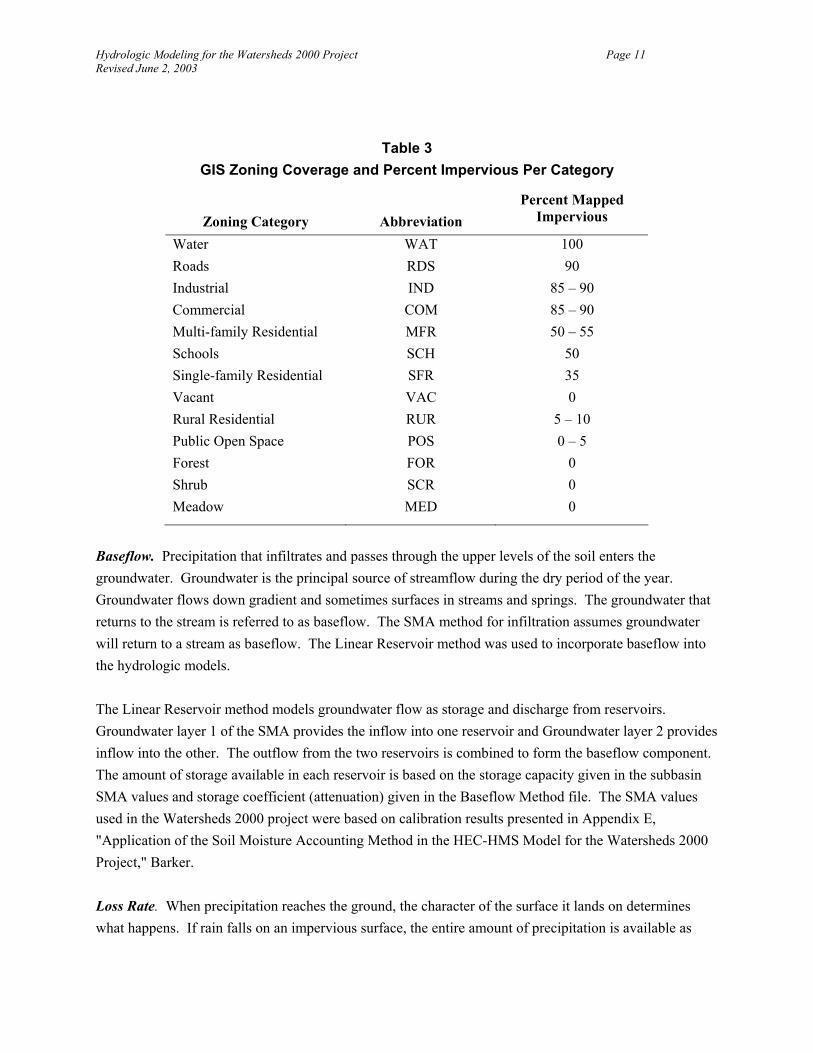
Hydrologic Modeling for the Watersheds 2000 Project Page 11 Revised June 2, 2003
Table 3 GIS Zoning Coverage and Percent Impervious Per Category
Zoning Category
Abbreviation
Percent Mapped Impervious
Water WAT 100 Roads RDS 90 Industrial IND 85 – 90 Commercial COM 85 – 90 Multi-family Residential MFR 50 – 55 Schools SCH 50 Single-family Residential SFR 35 Vacant VAC 0 Rural Residential RUR 5 – 10 Public Open Space POS 0 – 5 Forest FOR 0 Shrub SCR 0 Meadow MED 0
Baseflow. Precipitation that infiltrates and passes through the upper levels of the soil enters the groundwater. Groundwater is the principal source of streamflow during the dry period of the year. Groundwater flows down gradient and sometimes surfaces in streams and springs. The groundwater that returns to the stream is referred to as baseflow. The SMA method for infiltration assumes groundwater will return to a stream as baseflow. The Linear Reservoir method was used to incorporate baseflow into the hydrologic models. The Linear Reservoir method models groundwater flow as storage and discharge from reservoirs. Groundwater layer 1 of the SMA provides the inflow into one reservoir and Groundwater layer 2 provides inflow into the other. The outflow from the two reservoirs is combined to form the baseflow component. The amount of storage available in each reservoir is based on the storage capacity given in the subbasin SMA values and storage coefficient (attenuation) given in the Baseflow Method file. The SMA values used in the Watersheds 2000 project were based on calibration results presented in Appendix E, "Application of the Soil Moisture Accounting Method in the HEC-HMS Model for the Watersheds 2000 Project," Barker. Loss Rate. When precipitation reaches the ground, the character of the surface it lands on determines what happens. If rain falls on an impervious surface, the entire amount of precipitation is available as

Hydrologic Modeling for the Watersheds 2000 Project Page 12 Revised June 2, 2003
runoff. When precipitation falls on a pervious surface, the water is infiltrated into the soil. The soil will continue to infiltrate all the precipitation until the rate of rainfall is greater than the infiltration capacity of the soil, at which point runoff begins. The HMS program requires a loss rate method to effectively simulate the relationship between precipitation and infiltration. The loss rate used in this project is the Soil Moisture Accounting (SMA) method. The attached MGS report entitled, “Application of the Soil Moisture Accounting Method in the HEC-HMS Model for the Watersheds 2000 Project” (Appendix E), along with the section of this report titled ‘GIS Applications’, provides an overview of the SMA method and how the parameters were developed for this project. MGS provided SMA input parameters based on a calibration of two HSPF and HEC-HMS models to streamflow data for Bronson Creek and Fanno Creek. These parameter values were used as starting points or building blocks for an area-wide calibration that was based primarily on Fanno Creek flood flow data from 1994 through 1996. The Soil Moisture Accounting (SMA) module was used to account for the rainfall losses associated with infiltration and groundwater interaction. As described in the MGS report, the soil infiltration rate was calculated as the weighted average of all soil infiltration rates within each subbasin. All impervious area within the boundary was averaged using an infiltration rate of 0.0 in/hr. Using the average infiltration rates in the HMS model, the results were analyzed for runoff characteristics. It was discovered that in subbasins with infiltration rates above approximately 0.60 in/hr, the infiltration rate was always greater than the precipitation rate and therefore the subbasin never experienced surface run-off. This was true even for the 500-year storm event. In response to this issue, MGS conducted an investigation to determine when specific land use/ground cover types should start to produce surface run-off. “Development of Design Storms for the Portland Oregon Area” (Appendix B) contains a two-page analysis using calibrated HSPF models of Bronson and Fanno Creeks. The analysis determined that surface run-off for pasture ground cover begins during the 10-year storm event. Forest ground cover types should start to experience surface run-off during the 50-year storm event. Through the HMS analysis, it was discovered that in the southern region of the county, an infiltration rate of 0.45 in/hr would create surface run-off during the 10-year storm event and a rate of 0.50 in/hr would create surface run-off at the 50-year storm event. An infiltration rate of 0.55 in/hr would create run-off during the 100-year storm event. To ensure run-off was predicted correctly in subbasins for the larger storm events, subbasins with an infiltration rate above 0.45 in/hr, were reviewed for possible modifications. When the amount of pasture was greater than the amount of forest, the calculated infiltration rate was changed to 0.45 in/hr. When the amount of forest was greater than the amount of pasture, the infiltration rate was changed to either 0.50 or 0.55 in/hr. If the initial infiltration rate was above 1.0 in/hr, the infiltration rate was revised to 0.55 in/hr.

Hydrologic Modeling for the Watersheds 2000 Project Page 13 Revised June 2, 2003
If the initial infiltration rate was below 1.0 in/hr, the rate was revised to 0.50 in/hr. These revisions to the infiltration rates should provide for a more realistic run-off occurrence in underdeveloped subbasins. In the eastern portion of the county, MGS suggested a different set of parameter values based on whether the subbasin area was considered urban or rural. Using GIS, a “ruralness” ratio was calculated for each delineated subbasin area. The ruralness ratio is taken as forest area in the subbasin plus rural area in the subbasin divided by total subbasin area. If this “ruralness” is greater than 0.45, it was assumed to be a rural subbasin area. If this “ruralness” is less than or equal to 0.45, it was assumed to be an urban subbasin. The minimum infiltration rate for urban was adjusted downward to 0.05 in/hr from the MGS suggested 0.15 in/hr. The maximum remained at 0.20 in/hr as MGS suggested. The rural infiltration rate varied from 1.3 in/hr to 0.76 in/hr depending on specific soil conditions. When missing data was encountered, 0.75 in/hr was used. However, a unique weighting scheme was devised that computed an overall “raw” infiltration based on: the fraction of the subbasin that was rural, the fraction of the subbasin that was effectively impervious, and the fraction of the subbasin that was urban pervious. The final values of infiltration used for any given east region subbasin area was the result of the area-wide calibration using Fanno Creek data. A slope factor was introduced to reflect the fact that steeper areas will not be able to infiltrate as much water as the pure soil/cover characteristics may assume. This slope factor’s inclusion is instrumental in tracking the observed hydrographs during the early stages of an event. Reaches. Downstream routing of flow hydrographs through the watershed model is carried out using reaches. The reaches represent all forms of conveyance, including storm pipes, channels (ditches/streams), and reservoirs (ponds/lakes). For pipes and channels, the Muskingum-Cunge (MC) method was used to model the attenuation of the hydrograph because it is physically based. The MC method is based on the concepts of continuity and momentum and uses the reach channel geometry, slope, and Manning’s ‘n’ values to estimate water surface elevations and velocities in the channel. By dividing the channel into slices along the reach length, the MC method can account for storage volume within the channel and overbank area. The in-channel storage is capable of attenuating the flow hydrograph as the flow migrates downstream. The velocity calculated using the MC method is used to assist in determining the timing of combining hydrographs as new subbasins contribute flow to the reaches. This method requires data on channel slopes and cross-sections. Where survey data was unavailable, channel cross-sections were estimated from topographic maps and field reconnaissance. The channel slope was estimated using survey information or U.S. Geological Survey maps. The cross-section information is limited to the general shape of the cross-section and the roughness coefficient (Manning’s ‘n’ value).

Hydrologic Modeling for the Watersheds 2000 Project Page 14 Revised June 2, 2003
The roughness coefficient is affected by many characteristics of the channel. These include the material forming the channel, flow impediments within the channel such as vegetation and obstructions, irregularity of the channel in terms of size, shape, and cross section, and the amount of meandering in the channel. Determination of Manning’s ‘n’ for channel side slope and channel bottom must account for each of these variables. Tables 4 and 5 list Manning's ‘n’ used for urban streams and the Tualatin River.
Table 4 ‘N’ Values for Urban Streams
CHANNEL ‘n’ Values
Straight
Some Meandering
Extensive Meandering
Clean and lines .025 .03 .035 Clean bottom/light brush .05 .06 .07 Clean bottom and brush sides, full flow .07 .08 .09 Dense high weeds .08 .09 .10 Willows .10 .11 .12 OVERBANK ‘n’ Value Asphalt/concrete .02 Lawn/golf course .03 Pasture/field .035 Weedy .05 Heavy brush .07 Forest/trunks only .10 Forest/flooded branches .12 Willows .15 Landscaped yard .06 Fence/house (block w/higher ground)

Hydrologic Modeling for the Watersheds 2000 Project Page 15 Revised June 2, 2003
Table 5 ‘N’ Values for Large Rivers
CHANNEL (RIVER) ‘n’ Values
Straight
Some Meandering
Extensive Meandering
Clean, straight, full no rifts or deep pools 0.025 0.030 0.033 Same as above, but more stones and weeds 0.030 0.035 0.040 Clean, some pools and shoals 0.033 0.040 0.045 Same as above, but some weeds and stones 0.035 0.045 0.050 Same as above, but more stones 0.045 0.050 0.060 Sluggish reaches, weedy, deep pools 0.050 0.070 0.080 Very weedy reaches, deep pools, or floodways With heavy stands of timber and brush
0.075 0.100 0.150
OVERBANK (FLOODPLAIN) ‘n’ Value Pasture, no brush
1. Short grass 2. High grass
.030 .040
Cultivated areas 1. No crop 2. Mature row crops 3. Mature field crops
.030 .035 .040
Brush 1. Scattered brush, heavy weeds 2. Light brush and trees, in winter 3. Medium to dense brush, in winter
.050 .050 .070
Trees 1. Cleared land with tree stumps, no sprouts 2. Same as above, but heavy sprouts 3. Heavy stand of timber, a few down trees,
little undergrowth, flow below branches 4. Same as above, but with flow into branches 5. Dense willows
.040 .060 .100
.120 .150
Channel characteristics are best determined by a field visit and/or photographs. Both were performed for various locations along all of the study creeks. Roughness coefficients were calculated for channel side slopes and bottoms at all sample locations using methods from Open-Channel Hydraulics (Chow, 1959). Chow presents the following equation for calculating ‘n’:

Hydrologic Modeling for the Watersheds 2000 Project Page 16 Revised June 2, 2003
n = (n0+n1+n2+n3+n4)*m5
where,
no = a value based on the material forming the channel (values from 0.020 to 0.028)
n1 = a value based on the degree of irregularity of channel surface (values from 0.000 to 0.020)
n2 = a value based on the variation in channel cross section (values from 0.000 to 0.015)
n3 = a value based on flow obstructions (values from 0.000 to 0.060)
n4 = a value based on the presence of vegetation (values from 0.005 to 0.100)
m5 = a value based on the degree of meandering (values from 1.000 to 1.300)
Roughness coefficients calculated using this equation were compared to values previously established and documented in the Washington County Flood Insurance Study (FIS). The established data was limited, but numbers that were found compared favorably to those calculated by the above method. The photographs and field notes used in the Manning’s ‘n’ determination were also used to create eight-point cross sections. The coordinate orientation of the cross sections followed that of the project surveyors, meaning the X coordinate origin was the upper left-hand point of the channel and the Y coordinate origin was the left channel bottom, looking downstream. The channel geometry used to describe the reaches was taken from information gathered in the field. For each reach, the stream cross section geometry was noted as were the stream characteristics and vegetation growth. For inaccessible reaches, the RLIS topographic data as well as aerial photos were used to assist in estimating stream geometry. In most cases, stream cross sections were available from sections upstream and downstream of these sites and were used to develop a “best-fit” channel. In cases where a reach was a pipe, the pipe size was determined from field visits or by reviewing record drawings. Pipe slopes, if not given in the record drawings, were estimated from area topography. Reservoirs. Initially, the HMS models did not include any additional storage other than the in-channel storage volume calculated in the routing reaches using the Muskingum-Cunge method. During the development of the hydraulic models, areas of significant storage were discovered. At locations in the hydraulic models where there were large changes in water surface elevations across bridges or culverts, additional storage was entered into the HMS model. On the upstream side of the hydraulic structure, a stage versus area relationship was developed. From the hydraulic model, a rating curve was developed for the structure in question. The stage versus area

Hydrologic Modeling for the Watersheds 2000 Project Page 17 Revised June 2, 2003
relationship, along with the structure rating curve, were input into the HMS model as a reservoir. The HMS models were then rerun and new flows calculated. Calibration. Calibration data from multiple sources including NOAA-NWS, USGS, CWS/USA, and the Washington County Water Master were evaluated. In general, insufficient hourly rainfall and coincident hourly flow information was available to allow complete model calibration. Limited information was available for Fanno and Bronson Creeks and this was extrapolated throughout the basin. Typically, the models will require calibration and verification when good local data becomes available. The greatest flow event recorded for three stream gauges in the study area occurred on February 17, 1949. The event data is presented in “Statistical Summaries of Streamflow Data in Oregon” (USGS Report 84-454). The following is a summary of available data for the three gauges for that event:
• The Gales Creek stream gauge at Roderick Road (gauge 14204500) has the longest period of record of the three gauges and, with a tributary area of 66 square miles, accounts for the majority of the basin. The Washington County Flood Insurance Study (FIS) has the peak discharges at this location as 5,800 cubic feet per second (cfs); 8,150 cfs; 9,150 cfs; and 11,600 cfs for the 10-year, 50-year, 100-year and 500-year flood events, respectively. For the February 17, 1949 storm event, the measured peak flow at the Gales Creek gauge was 6,410 cfs. Hourly rainfall data for Gales Creek is available from the Glenwood 2 WNW rain gauge, located in the center of the Gales Creek basin.
• The stream gauge on the East Fork of Dairy Creek (gauge 14205500) is upstream of Highway 26 and has a tributary area of 43.0 square miles. Recorded peak flow at this gauge for the February 17, 1949 storm was 1,420 cfs. The East Fork of Diary Creek was not included in the detailed study area of the Washington County FIS. Rainfall data for this gauge is from the Buxton 5 E Meacham Ranch rain gauge, located in the center of the East Fork of Diary Creek basin.
• The stream gauge on McKay Creek (gauge 14206000) is upstream of Highway 26 and has a tributary area of 27.6 square miles. The peak flow at this location for the February 17, 1949 storm was 2,100 cfs. An evenly weighted rainfall curve was developed from the Buxton Meacham Ranch rain gauge and the Sauvie Island rain gauge.
The amount, type and level of detail in the available information does not allow for calibration of the models for Ash, Beaverton, Butternut, Cedar Mill, Cedar, Chicken, Council, Cross, Dairy, Dawson, Glencoe, Gordon, Hedges, Johnson South, Nyberg, Rock, Saum, South Rock, Storey, Summer, Thatcher, Waible, and Willow Creeks. Figures 4 through 11 present the final calibration graphs for four flood events recorded at two streamflow gauges on Fanno Creek. Each graph presents the observed streamflow data along with the simulated

Hydrologic Modeling for the Watersheds 2000 Project Page 18 Revised June 2, 2003
streamflow based on the new HEC-HMS model and the old HEC-1 model. It should be noted that several of the simulated peak flows were greater than those observed. This occurred because PWR simulated saturated soil conditions whereas those conditions did not exist when the actual flood event occurred. The most important aspect to glean from these calibrations is the timing of the observed versus the simulated peak flow. Most of the peaks match well in time. If a peak is simulated when one was not observed or the reverse, it is usually a problem with the single rainfall trace not being representative of what fell on the entire watershed. Overall the calibration was quite good. As part of the regional calibration based on the Fanno Creek data, all the raw subbasin lag times were increased by 40% throughout the entire East study area. Control Specifications
Data File Management. Separate basin models were developed for existing and future land use conditions for each basin in the study area. The models were named “existing” or “future.” The control specification defines the starting and ending date and time for the model to execute. It also specifies the time interval the model uses to evaluate the system. For all projects and models, the control specification used in this project was that of the precipitation information. The control specification was titled “Control 1.” Results The HEC-HMS models developed for the most of the study area are for watersheds with no available gauging information. Because of this, most of the hydrologic models presented, except where noted above, are not calibrated and are only estimates. Comparison analysis was conducted between the 72-hour storm used for this Watersheds 2000 project and the 24-hour SCS Type 1-A storm previously used for the Washington County Flood Insurance Study. This analysis was conducted on Fanno, Summer, Ash, Butternut, Rock, Dawson, Beaverton, Bronson, Willow, Cedar Mill, and Johnson Creeks. In the majority of cases, peak flows were significantly lower than the earlier modeling, with the exceptions of Beaverton, Dawson, and Rock Creek. (See PWR memorandum from Seth Jelen, P.E. to Kendra Smith dated April 30, 2002 found in Appendix A.) The implication associated with mostly lower peak flows is that flood elevations may decrease. However, because waterway roughness coefficients have dramatically increased over the last twenty years (i.e., FISs developed around 1980), flood elevations are liable to remain the same or slightly increase throughout the eastern study area. Another implication of these 72-hour flows is they probably should not be used for waterways whose drainage areas are less than a square mile. These small watersheds would obviously receive a much larger peak flow from a shorter duration early fall or summer type of an event.

Hydrologic Modeling for the Watersheds 2000 Project Page 19 Revised June 2, 2003
Estimated peak flow rates were generated for all of the subbasins within the study area for the existing and future conditions, respectively. In general, the difference between future and existing conditions is minimal. This is due to the fact that the study areas within the urban growth boundary are nearly completely developed and the areas outside the urban growth boundary are not expected to experience significant development. Appendix G details the estimated peak flow rates at the junctions (nodes) modeled in HEC-HMS for each watershed. The junctions represent locations within the watershed where flows from two or more sources (i.e., subbasins and reaches) are combined. The values are the results of adding the total hydrographs, not just the peaks. Peak flow rates for all the reaches in the study area were also modeled. The reaches represent conveyance of flow either for pipes, ditches, or streams. Since reaches represent streams, they have the ability to attenuate flow within the reach length. The attenuation occurs from available storage in overbank areas. Peak flows are calculated at the downstream end of the reach. The flow data resulting from the hydrologic analysis was used in the hydraulic analysis phase of the study. The flows were also used in separate capacity analyses for culverts throughout the watershed. A fish passage barrier analysis was conducted using data produced from this hydrologic analysis. This analysis is described in the companion to this paper "Hydraulic Modeling for the Watersheds 2000 Project," prepared by Clean Water Services. As noted previously, Clean Water Services is in the process of installing flow gauge stations throughout the Tualatin River watershed. Future data from the gauges will be used in the calibration and verification of the models prepared under this assignment. Suggested locations of gauge stations were provided to Clean Water Services from each of the regional consultants during the Watersheds 2000 project.

N
FIGURE 1Study Area Boundaries
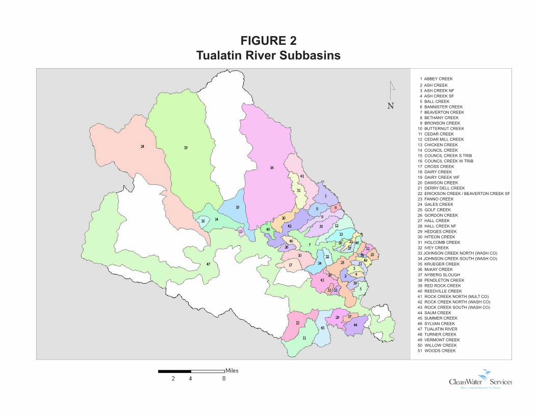
FIGURE 2Tualatin River Subbasins
1 ABBEY CREEK2 ASH CREEK3 ASH CREEK NF4 ASH CREEK SF5 BALL CREEK6 BANNISTER CREEK7 BEAVERTON CREEK8 BETHANY CREEK9 BRONSON CREEK
10 BUTTERNUT CREEK11 CEDAR CREEK12 CEDAR MILL CREEK13 CHICKEN CREEK14 COUNCIL CREEK15 COUNCIL CREEK S TRIB16 COUNCIL CREEK W TRIB17 CROSS CREEK18 DAIRY CREEK19 DAIRY CREEK WF20 DAWSON CREEK21 DERRY DELL CREEK22 ERICKSON CREEK / BEAVERTON CREEK SF23 FANNO CREEK24 GALES CREEK25 GOLF CREEK26 GORDON CREEK27 HALL CREEK28 HALL CREEK NF29 HEDGES CREEK30 HITEON CREEK31 HOLCOMB CREEK32 IVEY CREEK33 JOHNSON CREEK NORTH (WASH CO)34 JOHNSON CREEK SOUTH (WASH CO)35 KRUEGER CREEK36 McKAY CREEK37 NYBERG SLOUGH38 PENDLETON CREEK39 RED ROCK CREEK40 REEDVILLE CREEK41 ROCK CREEK NORTH (MULT CO)42 ROCK CREEK NORTH (WASH CO)43 ROCK CREEK SOUTH (WASH CO)44 SAUM CREEK45 SUMMER CREEK46 SYLVAN CREEK47 TUALATIN RIVER48 TURNER CREEK49 VERMONT CREEK50 WILLOW CREEK51 WOODS CREEK
N

FIGURE 3HMS Schematic for Nyberg Creek Model

Calibration - 20 February 1994 - Upper Fanno CreekFigure 4
0
50
100
150
200
250
300
60 65 70 75 80 85 90 95 100Hours into Event
Flow
(cfs
)
HMS at 56th AveObs at 56th AveHEC1 at 56th Ave

Calibration - 20 February 1994 - Lower Fanno CreekFigure 5
0
200
400
600
800
1000
1200
1400
60 70 80 90 100 110 120Hours into Event
Flow
(cfs
)
HMS at Durham RdObs at Durham RdHEC1 at Durham Rd

Calibration - 15 February 1995 - Upper Fanno CreekFigure 6
0
50
100
150
200
250
0 10 20 30 40 50 60 70Hours into Event
Flow
(cfs
)
HMS at 56th AveObs at 56th AveHEC1 at 56th Ave

Calibration - 15 February 1995 - Lower Fanno CreekFigure 7
0
200
400
600
800
1000
1200
0 10 20 30 40 50 60 70 80 90Hours into Event
Flow
(cfs
)
HMS at DurhamObs at Durham RdHEC1 at Durham Rd
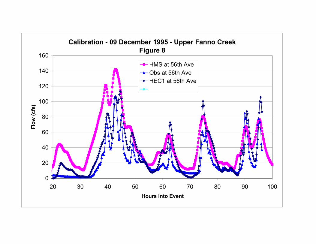
Calibration - 09 December 1995 - Upper Fanno CreekFigure 8
0
20
40
60
80
100
120
140
160
20 30 40 50 60 70 80 90 100Hours into Event
Flow
(cfs
)
HMS at 56th AveObs at 56th AveHEC1 at 56th Ave

Calibration - 09 December 1995 - Lower Fanno CreekFigure 9
0
100
200
300
400
500
600
700
800
900
0 20 40 60 80 100 120Hours into Event
Flow
(cfs
)
HMS at Durham RdObs at Durham RdHEC1 at Durham Rd

Calibration - 03 February 1996 - Upper Fanno CreekFigure 10
0
50
100
150
200
250
300
350
50 60 70 80 90 100 110 120 130 140 150Hours into Event
Flow
(cfs
)
HMS at 56th AveObs at 56th AveHEC1 at 56th Ave

Calibration - 03 February 1996 - Lower Fanno CreekFigure 11
0
200
400
600
800
1000
1200
1400
1600
1800
2000
50 60 70 80 90 100 110 120 130 140 150Hours into Event
Flow
(cfs
)
HMS at Durham RdObs at DurhamHEC1 at Durham

APPENDIX A
Memorandum from Seth Jelen, PE, PWR
to Kendra Smith, CWS April 2, 2002
PWR Recommends 24-Hour SCS1A Storm for Floodplain Remapping
We Think the World of Water
PACIFIC WATER RESOURCES, INC.
503.671.9709
fax: 503.671.0711 [email protected] www.pacificwr.com
4905 SW Griffith Drive, Suite 200, Beaverton, Oregon 97005
MEMORANDUM
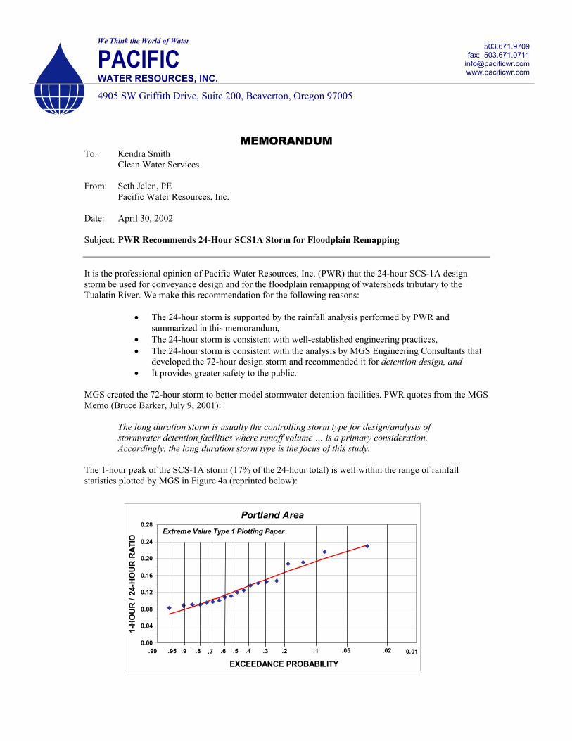
To: Kendra Smith Clean Water Services From: Seth Jelen, PE Pacific Water Resources, Inc. Date: April 30, 2002 Subject: PWR Recommends 24-Hour SCS1A Storm for Floodplain Remapping It is the professional opinion of Pacific Water Resources, Inc. (PWR) that the 24-hour SCS-1A design storm be used for conveyance design and for the floodplain remapping of watersheds tributary to the Tualatin River. We make this recommendation for the following reasons:
• The 24-hour storm is supported by the rainfall analysis performed by PWR and summarized in this memorandum,
• The 24-hour storm is consistent with well-established engineering practices, • The 24-hour storm is consistent with the analysis by MGS Engineering Consultants that
developed the 72-hour design storm and recommended it for detention design, and • It provides greater safety to the public.
MGS created the 72-hour storm to better model stormwater detention facilities. PWR quotes from the MGS Memo (Bruce Barker, July 9, 2001):
The long duration storm is usually the controlling storm type for design/analysis of stormwater detention facilities where runoff volume … is a primary consideration. Accordingly, the long duration storm type is the focus of this study.
The 1-hour peak of the SCS-1A storm (17% of the 24-hour total) is well within the range of rainfall statistics plotted by MGS in Figure 4a (reprinted below):
Portland Area
0.00
0.04
0.08
0.12
0.16
0.20
0.24
0.28
EXCEEDANCE PROBABILITY
1-HO
UR /
24-H
OUR
RAT
IO
.5 .05.3 .1 .02
Extreme Value Type 1 Plotting Paper
.4.6.8.9 .7.99 .95 0.01.2
Memorandum: PWR Recommends 24-Hour SCS1A Storm for Floodplain Remapping For reference, Appendix A (attached) compares in greater detail the three design storm distributions considered in this memorandum. The 24-hour SCS1A is most intense, while the two 72-hour distributions have increasing total volume with decreasing intensity. The ratios of 1-hour to 24-hour distributions are:
17% SCS-1A (24-hour) distribution (“storm”) 13% 72-hour (Summer) storm 12% 72-hour (Winter) storm – the “72-hour” storm modeled for Watersheds 2000
PWR concluded that large event depths can still have periods of intense rainfall – the intense peak within the SCS1A distribution is within the range of observed peak event intensities (as are both 72-hour distributions). We evaluated nearly 50 years of rainfall data from the Portland airport, grouped hourly rainfall into events and tabulated the peak rainfall for each over a range of durations ( (1, 2, 3, 4, 6, 12, 24, 36, 48, and 72 hours). We graphed points for the peak intensity in 72-hours versus that in 24-hours for each event, plus lines representing each of the three design storm distributions. We made similar graphs for 1-hour versus 6-hour, and for 1- and 6-hour versus 24-hour. The graphs are appended to this memorandum for reference as Appendix B. PWR concluded that the 24-hour SCS1A distribution better reflects shorter rainfall durations. We plotted observed rainfall event peaks versus those expected using the three distributions of established design depths. The plots show that the SCS1A storm matched the observed data while both 72-hour distributions were noticeably lower for durations less than 24 hours. For 72-hours, the smaller but more intense storm #1 (early peak) matched the observed rainfall much better than the larger storm #2. Note that by definition all three distributions are identical for the 24-hour duration. These graphs are attached as Appendix C. PWR concluded that the 24-hour SCS1A distribution is more consistent with the response times of the watersheds to large regional events. We found that these response times of the watersheds tributary to the Tualatin River were less than 24 hours. This time represents the difference in time between the peak of rainfall and the peak of runoff. Response time and peak flow both increase with increasing drainage area and length as one moves downstream in the watershed. These times were modeled along with the peak flows in the HMS models. Results are graphed in Appendix D. This is particularly important because watersheds tend to respond more strongly to rainfall of duration nearer their response time, much like a tuning fork resonates most strongly from sound near its own pitch. Because the probable rainfall intensity is higher as the duration is shorter, it is important that the design storm duration is kept comparable to the watershed response time. Otherwise, if the watershed responds much more slowly than the rainfall duration, the watershed will never have time to “fill up” before the rainfall stops. Or if the watershed responds more quickly, then the resulting flow would be too low. Finally, PWR concluded that the 24-hour SCS1A design storm distribution represents a safer, more conservative approach by Clean Water Services and cooperating jurisdictions for modeling flows for floodplain remapping and conveyance design. The 24-hour SCS1A design storm distribution is the one normally used and widely accepted in this region to design conveyance improvements and to model flows for flood insurance remapping. Moreover, there is a potential for liability if damage is sustained by the public that could have been reduced or avoided had the higher 24-hour peak flows been used. In summary:
• PWR recommends that the flows used in the Tualatin River itself be based on an analysis of observed peak flows at the USGS gaging stations along the river,
• PWR recommends that the 24-hour SCS1A design storm distribution (SCS1A) be used to model conveyance and FIS remapping flows for watersheds tributary to the Tualatin River,
• PWR recommends that the SCS1A be used for design of conveyance structures (culverts and bridges) within those tributary watersheds, and
• PWR recommends that the 72-hour storm # 2 be used for detention design, as its lower release rate and greater volume will better protect downstream areas from erosion and high flows.
April 30, 2002 Page 2 Pacific Water Resources, Inc.

APPENDIX B
MGS Engineering Consultants, Inc. July 9, 2001
Development of Design Storms for the Portland, Oregon Area

DEVELOPMENT OF DESIGN STORMS FOR THE PORTLAND OREGON AREA
7326 Boston Harbor Road NE Olympia, WA 98506 (360) 570-3450
July 9, 2001
1

DEVELOPMENT OF DESIGN STORMS FOR THE PORTLAND OREGON AREA
OVERVIEW Success in rainfall-runoff modeling using an event-based approach is dependent in-part upon utilizing a design storm that contains storm characteristics that are representative of the site of interest. In the Pacific Northwest, west of the Cascade Mountains, there are three distinctive categories of storm types. These storm types may be generally categorized as short duration, intermediate duration, and long duration storms11. Short duration storms are primarily warm season events. Periods of intense precipitation may last from 10-30 minutes with precipitation commonly occurring over a 1-6 hour period. These storms are limited in areal coverage but can produce high intensities over isolated areas. These storms are often termed thunderstorms as they are sometimes accompanied by thunder, lightning, and hail. They can produce very flashy flood hydrographs with a large flood peak, particularly in urban watersheds where much of the land surface is covered by imperious surfaces. The short duration storm is often the controlling storm type for sizing conveyance structures in urbanized areas. Intermediate durations storms can occur throughout the year but are most common in the fall to early-winter seasons. These storms often contain moderate to high intensities for a period of several hours, and precipitation commonly occurs over a 6-18 hour period. They can produce flood hydrographs that are flashy with a large peak discharge and a moderate runoff volume. Long duration storms are primarily late-fall and winter season events. These storms are characterized by low to moderate intensities and have durations varying from near 24-hours to over 72-hours. These storms are commonly intermittent in nature containing multiple periods of precipitation over several days. The long duration storms are associated with synoptic scale (continental scale) weather systems originating over the Pacific Ocean and precipitation commonly extends over very large areas. This type of storm typically produces floods with a sustained flood peak that is well supported by a large runoff volume. The long duration storm is usually the controlling storm type for design/analysis of stormwater detention facilities where runoff volume, in addition to flood peak discharge, is a primary consideration. Accordingly, the long duration storm type is the focus of this study. APPROACH TO STORM ANALYSIS The approach taken in this study is to develop design storms that incorporate those storm characteristics that can have a significant effect on the magnitude of the flood peak discharge and runoff volume, and can affect the shape of the flood hydrograph. Based on these considerations, storm characteristics of interest for long duration storms include11:
• shape of the hyetograph (macro storm pattern) • magnitude of incremental precipitation amounts within the storm • elapsed time to occurrence of the high intensity portion of the storm • sequencing of incremental precipitation amounts in the high intensity portion of storm • sequencing of incremental amounts in the period of maximum 24-hour precipitation
2

The analysis of each of these storm characteristics is presented in the sections that follow. DATABASE OF STORMS In analyzing storms, it is important to select storms from climatologically similar areas. Climatologic similarity refers to geographic areas that have similar physical and climatological characteristics and are subjected to similar meteorological conditions during storm events. The Portland Metropolitan area is bordered on the west by the Coast Mountains and to the east by the Cascade Mountains. Mean annual precipitation2,8 varies across Washington County, decreasing with elevation from the Coastal Mountains to a low near Hillsboro, and then increasing in magnitude progressing east from Portland into the foothills of the Cascade Mountains (Figure 1).
Figure 1 – Mean Annual Precipitation Map of the Watersheds 2000 Study Area (Oregon Climate Service8, Mean Annual Precipitation Map for Oregon,
PRISM Model, Corvallis Oregon, 1997)
For purposes of this study, climatologically similar areas were taken as the Willamette Valley, and lowland and foothill areas in the inter-mountain zone between the Coastal Mountains and Cascade Mountains in Oregon and Washington. This region is representative of lowlands areas with limited orographic influence. Seventy precipitation measurement stations ranging from near Longview, Washington to the north, to near Eugene, Oregon to the south were used in the analysis (Appendix A). The primary interest of this study is large (rare) storm events. Therefore, it was important to select a sample of storms that is most representative of the storm characteristics to be expected in the more severe storms. Prior experiences in the analyses of dimensionless depth-duration relationships for Pacific Northwest storms11,12 indicated that storms with large precipitation amounts at both the 24-hour and 72-hour durations should be examined. Therefore, separate analyses were conducted of characteristics associated with storms that were rare at the 24-hour and 72-hour durations. 3

The first step in assembling the catalog of storms was to set a threshold for selection of storms. If, the threshold is set too high, an insufficient number of storms will be available to provide a representative sample. Conversely, if the threshold is set too low, then common storms will be included that may not be representative of the more severe storm events. A threshold of a 10-year recurrence interval was chosen which represents a balance between these two considerations. The storm selection process proceeded by first assembling an annual maxima series of storm amounts and dates for each precipitation measurement station for both the 24-hour and 72-hour durations. A simple non-parametric plotting-position formula1,4 (Equation 1) was used to estimate the recurrence interval of each precipitation amount:
T = (N + 0.2) / ( i – θ ) (1) where: T is the recurrence interval in years; N is the record length of the annual maxima series; i the rank of the precipitation amount of interest for the annual maxima series data ranked in descending order; and θ is a fitting parameter that is typically taken to be 0.40 for distributions with moderate to high skewness, such as annual maxima precipitation data. Specifically, if a station had a record length of 40-years, then the four largest storms/dates would be selected as candidate storms for inclusion in the Storm Catalog. For extreme storm events, it was common that precipitation exceeded the 10-year recurrence interval threshold at multiple stations. In these cases, the hourly recording station where the storm was most rare was included in the Storm Catalog. These procedures resulted in a sample set of 19 storms at the 24-hour duration and 16 storms at the 72-hour duration. The list of stations, precipitation amounts, and associated dates of the storms used to develop the design storm temporal patterns are shown in Tables 1 and 2 for storms that were rare at the 24-hour and 72-hour durations, respectively.
Table 1 –Catalog of Storms that Exceeded the 10-Year Recurrence Interval at the 24-Hour Duration
Station ID
Station Name
Storm Date
24-Hour Precipitation Amount
(in) 35-6749 Portland River Forecast Center 12/26-28/1942 2.78 35-6751 Portland International Airport 11/17-18/1946 2.55 35-7127 Rex 1 S 02/09-10/1949 3.34 35-5213 Marcola 11/21-23/1953 4.86 35-2709 Eugene Mahlon Sweet Airfield 12/18-21/1955 4.82 35-2867 Fern Ridge Dam 11/23-24/1960 4.00 35-5213 Marcola 02/09-10/1961 5.21 35-2374 Dorena Dam 11/21-24/1961 5.75 45-4769 Longview 11/19-20/1962 5.41 35-0673 Bellfountain 01/12-16/1974 4.94 35-1222 Buxton 12/12-15/1977 4.40 35-8884 Vernonia 2 10/05-06/1981 4.00 35-2709 Eugene Mahlon Sweet Airfield 12/05-06/1981 5.15 35-5213 Marcola 02/11-13/1984 4.71 45-4769 Longview 02/21-23/1986 4.70 35-4238 Jefferson 12/01-03/1987 3.40 35-1643 Clatskanie 01/06-09/1990 4.30 35-6751 Portland International Airport 10/26-27/1994 4.44 35-6751 Portland International Airport 11/18-19/1996 3.98
4
Table 2 –Catalog of Storms that Exceeded the 10-Year Recurrence Interval at the 72-Hour Duration
Station ID
Station Name
Storm Date
72-Hour Precipitation Amount
(in) 35-7500 Salem WSO Airport 02/16-18/1949 5.22 35-2374 Dorena Dam 10/26-29/1950 9.25 35-2867 Fern Ridge Dam 11/15-17/1950 5.87 35-2709 Eugene Mahlon Sweet Airfield 12/18-21/1955 8.18 35-5213 Marcola 02/09-10/1961 7.74 35-2374 Dorena Dam 11/21-24/1961 8.83 35-5050 Lookout Point Dam 12/19-23/1964 9.00 35-4603 La Comb 1 WNW 01/27-29/1965 5.20 35-0673 Bellfountain 01/12-16/1974 8.49 35-2709 Eugene Mahlon Sweet Airfield 12/01-04/1980 8.29 35-7586 Scoggins Dam 2 12/14-17/1982 5.50 35-1643 Clatskanie 01/06-09/1990 6.90 35-1643 Clatskanie 04/03-05/1991 7.20 35-6751 Portland International Airport 10/26-27/1994 5.10 35-3047 Foster Dam 02/05-08/1996 6.30 35-6751 Portland International Airport 11/18-19/1996 4.56
It should be noted that the elapsed time of precipitation of historical storms, from initial onset of precipitation to the final cessation of precipitation, varied from near 24-hours to greater than 72-hours. The selections of the 24-hour and 72-hour durations are conventional choices for evaluation of storm amounts and temporal characteristics. References to 24-hour and 72-hour durations in the remainder of the report are always meant to indicate storms where the precipitation amounts are more rare than a 10-year event at those specific durations. ANALYSIS OF STORM TEMPORAL CHARACTERISTICS Shape of the Hyetograph (Storm Macro Pattern) The general shape of historical hyetographs was analyzed by categorization of the hyetographs into one of twelve generalized storm macro patterns11 (Figure 2). As with any generalized categorization system, latitude and judgment are required in assigning historical hyetographs to one of the generalized patterns. This analysis provided a crude measure of the more frequently occurring storm macro patterns. As an initial measure of hyetograph shape, the frequency of occurrence of continuous versus intermittent patterns was computed. It was found that the majority of storms had intermittent macro patterns, with 63% of the storms at the 24-hour duration, and 75% of the storms at the 72-hour duration exhibiting intermittent patterns. Therefore, it is more likely to experience a sequence of storm events and intervening dry periods rather than continuous precipitation during long duration storms. The frequency of occurrence of observed storm macro patterns for the 24-hour and 72-hour durations are shown in Tables 3a and 3b, respectively. The frequency of occurrence for the combined sample of storms is shown in Table 3c. It can be concluded that the shapes of hyetographs are highly variable with patterns I, VII, and XII being somewhat more common than other patterns. These results for the Portland area are consistent with findings throughout the Pacific Northwest9,11 that indicate hyetographs exhibit a wide variety of storm macro patterns.
5

Figure 2 – Categorization of Hyetographs into Twelve General Macro Patterns
6

Table 3a – Frequency of Occurrence of Storm Macro Patterns at the 24-Hour Duration
I II III IV V VI VII VIII IX X XI XII 26% 4% 4% 11% 26% 4% 4% 21%
Table 3b – Frequency of Occurrence of Storm Macro Patterns at the 72-Hour Duration
I II III IV V VI VII VIII IX X XI XII 13% 6% 13% 13% 25% 13% 6% 13%
Table 3c – Combined Frequency of Occurrence of Storm Macro Patterns
I II III IV V VI VII VIII IX X XI XII 21% 7% 11% 11% 25% 7% 4% 14%
Examples of historical hyetographs are depicted in Figures 3a,b,c and in Appendix B.
Figure 3a – Hyetograph for Storm of January 12-15, 1974 at Bellfountain Oregon
Figure 3b – Hyetograph for Storm of February 10-12, 1949 near Rex Oregon
HYETOGRAPH
0.00
0.05
0.10
0.15
0.20
0.25
0.30
0 12 24 36 48 60 72 84 96 108 120TIME (Hours)
PREC
IPIT
ATIO
N (in
)
Macro Pattern I
1.17 inches 6-Hours
3.51 inches 72-Hours3.34 inches 24-Hours
Macro Pattern VII
2.21 inches 6-Hour
8.49 inches 72-Hour4.94 inches 24-Hour
HYETOGRAPH
0.00
0.10
0.20
0.30
0.40
0.50
0.60
0 12 24 36 48 60 72 84 96 108 120TIME (Hours)
PREC
IPIT
ATIO
N (in
)
7

HYETOGRAPH
0.000.05
0.100.150.20
0.250.30
0.350.40
0 12 24 36 48 60 72 84 96 108 120TIME (Hours)
PREC
IPIT
ATIO
N (in
)
Macro Pattern XII
1.56 inches 6-Hours
7.74 inches 72-Hours
5.21 inches 24-Hours
Figure 3c – Hyetograph for Storm of February 10-12, 1961 at Marcola Oregon Magnitude of Incremental Precipitation Amounts within the Storm The magnitudes of the incremental precipitation amounts within storms are important characteristics of hyetographs and design storms. In particular, the magnitude of the maximum incremental amounts for the high-intensity portion of the storm is a critical factor in determining the magnitude of the flood peak discharge in small urbanized watersheds. Tables 4a and 4b list the sample statistics for various interdurations within the long duration storms. The sample statistics for the shortest interdurations include minor adjustments (Weiss19) to account for recording of data on fixed intervals. The statistics are expressed as dimensionless ratios of the maximum 24-hour precipitation to allow comparisons to be made between storms9,11,15. For example, the sample mean of 0.132 for the 1-hour interduration (Table 4a) indicates that the maximum 1-hour precipitation amount during a long duration storm is, on-average, 13.2% of the maximum 24-hour precipitation amount for that storm. Table 4a – Sample Statistics for Ratios of the Maximum 24-Hour Precipitation Amount for Interdurations for Storms More Rare than the 10-Year Event at the 24-Hour Duration (sample statistics for storms contained in Table 1)
1-hr 2-hr 3-hr 6-hr 9-hr 12-hr 18-hr 30-hr 36-hr 42-hr 48-hr 54-hr 60-hr 66-hr 72-hrMean 0.132 0.196 0.253 0.404 0.515 0.631 0.848 1.096 1.162 1.210 1.245 1.253 1.303 1.342 1.392 Std Dev 0.045 0.056 0.063 0.067 0.066 0.069 0.057 0.059 0.108 0.139 0.147 0.146 0.160 0.198 0.243 Skew 1.00 1.37 1.04 0.96 0.83 0.71 -0.11 0.67 0.22 0.36 0.37 0.36 -0.08 0.22 0.23 Table 4b – Sample Statistics for Ratios of the Maximum 24-Hour Precipitation Amount for Interdurations for Storms More Rare than the 10-Year Event at the 72-Hour Duration (sample statistics for storms contained in Table 2)
1-hr 2-hr 3-hr 6-hr 9-hr 12-hr 18-hr 30-hr 36-hr 42-hr 48-hr 54-hr 60-hr 66-hr 72-hrMean 0.116 0.178 0.239 0.397 0.513 0.634 0.841 1.114 1.210 1.321 1.410 1.456 1.520 1.595 1.663 Std Dev 0.023 0.030 0.038 0.062 0.074 0.086 0.069 0.071 0.123 0.184 0.216 0.240 0.236 0.257 0.316 Skew 0.22 -0.15 -0.08 0.67 0.76 0.59 -0.02 0.43 0.12 -0.23 -0.33 0.02 0.01 -0.15 0.36
8
A review of the sample statistics provides some insights into the behavior of storms that are rare at the 24-hour and 72-hour durations. Ratios at the 1-hour and 2-hour interdurations for storms that are rare at the 24-hour duration (Table 4a) are larger and more variable than corresponding 1-hour and 2-hour ratios for storms that are severe at the 72-hour duration (Table 4b). This

indicates that long duration storms that have unusually large precipitation amounts at the 72-hour duration tend to have smaller short-duration ratios relative to storms that are rare at the 24-hour duration. This behavior is graphically depicted in the probability-plots shown in Figures 4a and 4b for the 1-hour interduration ratio data. Selection of mean values of the interduration ratio values would be appropriate for developing design storms that are representative of typical conditions experienced in severe storms. If more conservative design storms were desired, it would be appropriate to use larger interduration ratio values that are representative of more unusual conditions. These would correspond to using a 1-hour interduration ratio of perhaps 0.165, which has an exceedance probability of 0.20 (Figure 4a), 1 chance in 5 of being exceeded during a severe storm. The interduration ratio characteristics shown in Tables 4a and 4b will be used later in the assembly of design storms.
Portland Area
0.00
0.04
0.08
0.12
0.16
0.20
0.24
0.28
EXCEEDANCE PROBABILITY
1-HO
UR /
24-H
OUR
RAT
IO
.5 .05.3 .1 .02
Extreme Value Type 1 Plotting Paper
.4.6.8.9 .7.99 .95 0.01.2
Figure 4a – Probability-Plot of 1-Hour Interduration Ratios for Storms that are Rare at the 24-Hour Duration
Portland Area
0.00
0.04
0.08
0.12
0.16
0.20
0.24
0.28
EXCEEDANCE PROBABILITY
1-HO
UR /
24-H
OUR
RAT
IO
.5 .05.3 .1 .02
Extreme Value Type 1 Plotting Paper
.4.6.8.9 .7.99 .95 0.01.2
Figure 4b – Probability-Plot of 1-Hour Interduration Ratios for Storms that are Rare at the 72-Hour Duration
9

Elapsed Time to Occurrence of the High Intensity Portion of the Storm The elapsed time to the occurrence of the high-intensity portion of the storm affects both the magnitude of the flood peak discharge and the shape of the flood hydrograph. When the highest-intensities occur near the end of the storm (back-loaded storm), surface infiltration rates are likely to be lower due to wetting of the soil from prior precipitation. All other factors being equal, this generally results in higher runoff rates and larger flood peak discharges. With regard to stormwater detention facilities, a back-loaded storm results in the flood peak arriving after the detention pond is partially filled from prior runoff. This situation generally results in more stringent conditions for storage and passage of floodwaters. Thus, the elapsed time to the high-intensity portion of the storm can be an important factor in assembly of design storms. No significant differences were found between the sample statistics for the elapsed time to peak intensity data for the 24-hour and 72-hour durations. Therefore, the data were combined and the combined data had a mean value of 34.0 hours and a standard deviation of 14.8 hours. A probability-plot of the combined data is shown in Figure 5 where it is seen that storms exhibited time to peak intensity values ranging from 12-hours to 66-hours. This is companion information to the results of the macro pattern analysis, which reinforces the conclusion that storms occur in widely varying temporal patterns. Portland Area
0
12
24
36
48
60
72
EXCEEDANCE PROBABILITY
ELAP
SED
TIM
ETO
PEA
K IN
TEN
SITY
(Hou
rs)
.5 .05.3 .1 .02
Extreme Value Type 1 Plotting Paper
.4.6.8.9 .7.99 .95 0.01.2
Figure 5 – Probability-Plot of Elapsed Time to Peak Intensity in Long Duration Storms in the Portland Area Sequencing of Incremental Precipitation Amounts in the High Intensity Portion of Storm The sequence order of the incremental precipitation amounts during the high intensity portion of the storm can affect the magnitude of the resultant flood peak discharge. Herein, the sequence numbers 1, 2 and 3 refer to the largest, 2nd largest and 3rd largest 1-hour incremental precipitation amounts during the largest 6-hour block of precipitation in the long duration storm. Six sequences are possible: 123; 132; 213; 312; 231; and 321. The results from the analysis of storms for both the 24-hour and 72-hour durations were similar and Table 5 lists the results from the analysis of the combined data. It is seen in Table 5 that sequences where the largest 1-hour amount is sandwiched between the 2nd and 3rd largest amounts represent nearly half (47%) of the possible sequences. Thus, pattern 213 would be considered the more representative sequence for assembly of design storms.
10

Table 5 – Frequencies of Various Sequences of Three Largest 1-Hour Precipitation Increments within the Largest 6-Hour Precipitation Increment for the Portland Area
Sequence 123 132 213 312 231 321 Frequency 25% 4% 29% 18% 4% 21%
Sequencing of Incremental Amounts in the Period of Maximum 24-Hour Precipitation The sequence order of the incremental precipitation amounts during the greatest 24-hour period of precipitation also affects the magnitude of the resultant flood peak discharge. Here, the sequence numbers 1, 2, 3 and 4 refer to the largest, 2nd largest. 3rd largest and 4th largest 6-hour incremental precipitation amounts during the greatest 24-hour block of precipitation in the 72-hour storm. Given the four sequence numbers, there are 24 possible sequences. However, there were insufficient data to estimate the frequencies of all 24 combinations. Therefore, four basic sequences were examined that emphasized the location of the largest 6-hour increment of precipitation (i.e. 1xxx , x1xx , xx1x , xxx1 ). Sequence 1 has the largest 6-hour block occurring first and sequence two has the largest 6-hour block occurring from the 7th to the 12th hour in the 24-hour sequence, etc. As before, results from analysis of the 24-hour and 72-hour durations are very similar and the data were combined. Table 6 lists the results of the analysis of the combined 24-hour and 72-hour duration data. Sequence xx1x is seen to be the most common sequence, where the largest 6-hour block of precipitation occurs somewhere in the 13th through 18th hour of the maximum 24-hour precipitation amount.
Table 6 – Frequencies for Location of Largest 6-Hour Precipitation Increments within the Largest 24-Hour Precipitation Increment for the Portland Area
Sequence 1xxx x1xx xx1x xxx1 Frequency 14% 14% 50% 22%
Seasonality of Storms The term seasonality of storms is intended to describe the frequency of occurrence of storms that have exceeded the 10-year recurrence interval threshold. It is common knowledge in the Portland area that long duration storms are late-fall and winter storm events. However, situations sometimes arise where flood analyses are needed very early, or very late in the winter storm season. Seasonality information is useful in these situations in determining how early or late in the winter storm season could a long duration severe storm be considered a plausible occurrence. Likewise, the seasonality information is helpful in selection of realistic antecedent soil moisture conditions for the flood analyses. In general, the 24-hour and 72-hour duration seasonality data are similar in the Pacific Northwest. Prior studies11,12,14 indicate that 24-hour seasonality data have a mean value about 2-weeks earlier in the winter storm season and have slightly higher variance relative to 72-hour duration seasonality data. Thus, storms that are rare at the 24-hour duration occur over a slightly wider range of months in the winter storm season than storms that are rare at the 72-hour duration. The seasonality analyses were conducted using the same approach that was used for assembly of the catalog of extreme storms (Tables 1 and 2). Annual maxima precipitation data series were
11
assembled for the 70 stations listed in Appendix A. All storm amounts that exceeded a 10-year event were identified and the dates of the events were recorded and duplicates removed. This provided 32 storms for the 24-hour duration and 19-storms for the 72-hour duration. Numeric storm dates were then computed in terms of decimal months based on the calendar date of occurrence. For example, September 1st corresponds to 9.00, December 31st equates to 12.97, and February 15th equates to 14.50. Sample statistics were computed for the numeric dates and are listed in Table 7. Figures 6a,b depict probability-plots of the seasonality data where the historical data are seen to be nearly Normally distributed and spans the range from early-October through early-April.
Table 7 – Sample Statistics for Seasonality of Storms that Exceed a 10-Year Event at the 24-Hour and 72-Hour Durations
Sample Statistic 24-Hour Duration Storms 72-Hour Duration Storms Mean 12.69 (late-December) 12.84 (late-December) Standard Deviation 1.47 months 1.37 months Coefficient of Skewness 0.3 0.6
Portland Study Area
9.0
10.0
11.0
12.0
13.0
14.0
15.0
16.0
17.0
18.0
NON-EXCEEDANCE PROBABILITY
NU
MER
ICAL
STO
RM
DAT
E
.5 .98.7 .9 .999.99.95
Normal Plotting Paper
.02 .05 .8.6.4.2.1 .3.001 .01
Storms Rare at the 24-Hour Duration
Figure 6a – Probability-Plot of Seasonality Data for 24-Hour Duration Storms
Normal Distribution
Normal Distribution
Portland Study Area
9.0
10.0
11.0
12.0
13.0
14.0
15.0
16.0
17.0
18.0
NON-EXCEEDANCE PROBABILITY
NU
MER
ICAL
STO
RM
DAT
E
.5 .98.7 .9 .999.99.95
Normal Plotting Paper
.02 .05 .8.6.4.2.1 .3.001 .01
Stroms Rare at the 72-Hour Duration
Figure 6b – Probability-Plot of Seasonality Data for 72-Hour Duration Storms
12

ASSEMBLY OF DESIGN STORM TEMPORAL PATTERNS In reviewing the prior sections, it should be apparent that historical storms exhibit a wide variety of temporal characteristics. Given the high degree of natural variability, it is not reasonable to expect that a single design storm could be developed that would be representative of “typical” conditions. In fact, given the high degree of natural variability (see Figures 3a,b,c and Appendix B), a hyetograph labeled as typical would be a misnomer. At the same time, it could be cumbersome for practicing engineers and the regulatory community if a large suite of design storms were to be utilized in the design/analysis of stormwater facilities. Given these competing considerations, two synthetic design storms were developed for the study area. Each of the two design storms were developed in a manner that reasonably reflects the temporal characteristics observed in historical storms from areas climatologically similar to the Portland Metropolitan area. This was accomplished by utilizing storm temporal characteristics that have been observed with reasonably high frequencies of occurrence in historical storms. Each of these two design storms has a total duration of 72-hours to account for precipitation that occurs prior to and posterior to the maximum 24-hour precipitation amount. Portland Design Storm 1 The first design storm (Figure 7) is labeled Portland Design Storm 1 (PDS1) and contains higher short-duration intensities and lower total volume than the second design storm. The temporal characteristics of this storm are based on the characteristics observed in the analysis of storms that were rare at the 24-hour duration. This storm is intended for use on watersheds where the flood peak discharge in a winter long-duration storm is anticipated to be the controlling design event. Such watersheds could be characterized as being highly urbanized with few stormwater ponds, lakes or wetlands. The temporal characteristics contained in this storm are listed in Table 8 and the dimensionless ordinate values are listed in Appendix C.
Portland Design Storm 1
0.00
0.01
0.02
0.03
0.04
0.05
0.06
0.07
0.08
0 6 12 18 24 30 36 42 48 54 60 66 72TIME (Hours)
RATI
O T
O 2
4-HO
UR A
MO
UNT 30-minute increments
Figure 7 – Portland Area Design Storm 1
13

Table 8 – Temporal Storm Characteristics used in Assembly of Portland Design Storm 1
TEMPORAL CHARACTERISTICS SELECTED VALUE Storm Macro Pattern Intermittent – front loaded Elapsed Time to Peak Intensity 27-hours Magnitude of Incremental Precipitation Amounts Mean Values (Table 4a) Sequence of Hourly Amounts for High Intensity Portion of Storm 213 Sequencing of 6-Hour Amounts in Maximum 24-Hour Period 4312
Portland Design Storm 2 The second design storm (Figure 8) is labeled Portland Design Storm 2 (PDS2) and has smaller peak intensity than PDS1, but has a larger total volume. The temporal characteristics of this storm are based on the characteristics observed in the analysis of storms that were rare at the 72-hour duration. This second storm would likely be the controlling storm for watersheds where the total runoff volume, in addition to peak discharge, is an important factor. Such watersheds could be characterized as having relatively large amounts of hydraulic storage and lesser amounts of impervious surfaces. PDS 2 is anticipated to be the controlling storm for the design/analysis of stormwater detention facilities. The temporal characteristics contained in this storm are listed in Table 9 and the dimensionless ordinate values are listed in Appendix C.
30
TI
Portland Design Storm 2
0.00
0.01
0.02
0.03
0.04
0.05
0.06
0.07
0.08
0 6 12 18 24 36 42 48 54 60 66 72ME (Hours)
RATI
O T
O 2
4-HO
UR A
MO
UNT 30-minute increments
Figure 8 – Portland Area Design Storm 2 Table 9 – Temporal Storm Characteristics used in Assembly of Portland Design Storm 2
TEMPORAL CHARACTERISTICS SELECTED VALUE Storm Macro Pattern Intermittent – back loaded Elapsed Time to Peak Intensity 54-hours Magnitude of Incremental Precipitation Amounts Mean Values (Table 4b) Sequence of Hourly Amounts for High Intensity Portion of Storm 213 Sequencing of 6-Hour Amounts in Maximum 24-Hour Period 4312
14

APPLICATION OF DESIGN STORMS Ordinate values of the design storms were developed as ratios to the 24-hour precipitation amount to allow scaling from commonly available sources of precipitation magnitude-frequency information such as NOAA Atlas 27. Use of the design storms in rainfall-runoff modeling is accomplished by multiplying each dimensionless ordinate value (Appendix C) by the 24-hour amount for the recurrence interval of interest. This yields a scaled hyetograph on a 30-minute time step. Figures 9a and 9b depict examples of design storms scaled by a 24-hour, 100-year precipitation amount. Comparison with Previous Design Storm used in the Portland Area The SCS Type 1A17,18 synthetic storm has been used by engineers for rainfall-runoff modeling for many years for sites along the west coast of the United States. Limited documentation exists on the methods used for derivation of this storm (circa 1960’s). Based on numerous discussions with US Department of Agricultural Engineers and National Weather Service personnel, it appears that the storm was developed from a limited sample of storms recorded along the west coast of the US. The procedure for storm assembly apparently incorporated ratio methods that were common practice in the 1950’s and 1960’s. In that approach, a 10-year storm would be created by incorporating precipitation amounts for durations ranging from 30-minutes to 24-hours where each precipitation amount for each duration corresponded to a 10-year recurrence interval. That procedure ignores the seasonalities of storm types, and lumps storm characteristics that arise from various storm types. Oftentimes, storms that are producing the unusual short duration intensities are occurring during seasons that are different from the storms that produce the precipitation for the longer durations. These past procedures are not appropriate where storm types, and associated durations have differing seasonalities, such as the case in the Pacific Northwest11. Since the SCS Type 1A synthetic storm has been a commonly used method in the Pacific Northwest, it is worthwhile to compare the SCS Type 1A storm with the two design storms that were developed based on the temporal characteristics in the Portland area. Figures 9a and 9b depict comparisons between the SCS Type 1A storm and Portland Design Storms 1 and 2. These comparisons were made for Hillsboro Oregon and all three storms have been scaled by the 100-year 24-hour precipitation amount that is estimated to be 4.00 inches at Hillsboro. Comparisons of precipitation amounts for various interdurations within the storms are listed in Table 10. It should be noted that the total 72-hour precipitation amount in these design storms is 139.1% of the 24-hour precipitation amount for Portland Design Storm 1 (PDS1), and 166.1% of the 24-hour amount for Portland Design Storm 2 (PDS2). Table 10 – Comparison of Interduration Precipitation Amounts for Design Storms Containing a 24-Hour Precipitation Amount of 4.00 Inches
Interduration
SCS Type 1A
Portland Design Storm 1
Portland Design Storm 2
15-min 0.26 in 0.15 in 0.13 in 30-min 0.46 in 0.30 in 0.26 in 1-hour 0.68 in 0.53 in 0.46 in 2-hour 1.00 in 0.78 in 0.71 in 6-hour 1.84 in 1.62 in 1.59 in
12-hour 2.72 in 2.52 in 2.54 in 24-hour 4.00 in 4.00 in 4.00 in 48-hour 4.00 in 4.98 in 5.64 in 72-hour 4.00 in 5.57 in 6.65 in
15

It is seen in Figures 9a and 9b that the maximum intensities in the new design storms are noticeably less than those in the SCS Type 1A storm. A review of the findings in Table 4a, 4b and the historical storms depicted in Figures 3a,b,c and Appendix B show these intensities are consistent with intensities in the large storm events applicable to the Portland area. Further review of hyetographs in Figures 3a,b,c and Appendix B demonstrates the high frequency of occurrence of multi-day storm events. In particular, storms that have large precipitation amounts at the 24-hour duration are very likely to be multi-day events where the maximum 24-hour precipitation total is embedded within a longer precipitation event.
Design Storms Containing 100-Year 24-Hour Precipitation
0.000.100.200.300.400.500.600.700.800.901.001.10
0 12 24 36 48 60 72TIME (Hours)
INTE
NSIT
Y (in
/hr)
Portland Design Storm 1
Hillsboro Oregon
Figure 9a – Comparison of SCS Type 1A Synthetic Storm with Long Duration Portland Design Storm 1 for Hillsboro Oregon
SCS Type IA
SCS Type IA
Design Storms Containing 100-Year 24-Hour Precipitation
0.000.100.200.300.400.500.600.700.800.901.001.10
0 12 24 36 48 60 72TIME (Hours)
INTE
NSIT
Y (in
/hr)
Portland Design Storm 2
Hillsboro Oregon
Figure 9b – Comparison of SCS Type 1A Synthetic Storm
with Long Duration Portland Design Storm 2 for Hillsboro Oregon
16

SUMMARY Two design storms have been developed for the Portland area based on the temporal characteristics of historical storms that have been recorded in areas climatologically similar to the Portland Metropolitan area. The first design storm labeled Portland Design Storm 1 (PDS1) was developed based on the storm temporal characteristics that have been observed to occur most frequently in storms that were rare at the 24-hour duration. Portland Design Storm 2 (PDS2) was developed based on the storm temporal characteristics that have been observed to occur most frequently in storms that were rare at the 72-hour duration. It is expected that Portland Design Storm 2, which contains a larger 72-hour precipitation total, will be the controlling storm type for design/analysis of stormwater detention facilities where runoff volume, in addition to flood peak discharge, is a primary consideration.
17

REFERENCES 1. Cunnane C, Unbiased Plotting Positions - A Review, Journal of Hydrology, 37, 205-222, 1978.
2. Daly C, PRISM, Parameter-Elevation Regression on Independent Slopes Model, Oregon State University, Oregon Climate Service, 1994.
3. Frederick RH , Miller JF, Richards, FP, and Schwerdt RW, Interduration Precipitation Relationships for Storms – Western United States, Technical Report NWS 27, U.S. Dept. of Commerce, NOAA, National Weather Service, Washington DC, 1981.
4. Gringorten II, A Plotting Rule for Extreme Probability Paper, Journal of Geophysical Research, 68(3), 813-814, 1963.
5. Hosking JRM, and Wallis JR, Regional Frequency Analysis - An Approach Based on L-Moments, Cambridge Press, 1997.
6. HydroSphere, Climate Data, HydroSphere Data Products, Boulder CO.
7. Miller JF, Frederick RH and Tracey RS, NOAA ATLAS 2, Precipitation-Frequency Atlas of the Western United States, U.S. Dept. of Commerce, NOAA, National Weather Service, Washington DC, 1973.
8. Oregon Climate Service, Mean Annual Precipitation Maps for Western United States, PRISM Model, Corvallis Oregon, 1997.
9. Parrett C, Characteristics of Extreme Storms in Montana and Methods for Constructing Synthetic Storm Hyetographs, USGS, Water Resources Investigations Report 98-4100, Helena Montana, July 1998.
10. Schaefer MG, Regional Analyses of Precipitation Annual Maxima in Washington State, Water Resources Research, Vol.26, No.1, pp119-132, January 1990.
11. Schaefer MG, Characteristics of Extreme Precipitation Events in Washington State, Washington State Dept. of Ecology, Report 89-51, October 1989.
12. Schaefer MG, Magnitude-Frequency Characteristics of Precipitation Annual Maxima in Southern British Columbia, MGS Engineering Consultants, Inc., prepared for BChydro Power Supply and Engineering, December 1997.
13. Schaefer, MG, Precipitation Magnitude-Frequency Characteristics for the American River Watershed, MGS Engineering Consultants, Inc., prepared for US Army Corps of Engineers Hydrologic Engineering Center, January 2000.
18

14. Schaefer, MG, Seasonality Analysis of Extreme Storms for the American River Watershed, MGS Engineering Consultants, Inc., prepared for US Army Corps of Engineers Hydrologic Engineering Center, November 1999.
15. Schaefer MG and Barker BL, Stochastic Modeling of Extreme Floods for Keechelus Dam,
MGS Engineering Consultants, September 1999. 16. Stedinger, JR, Vogel RM, and Foufoula-Georgiou, E, Frequency Analysis of Extreme
Events, Chapter 18, Handbook of Hydrology, McGraw Hill, 1992.
17. US Soil Conservation Service, Hydrology, National Engineering Handbook, Section 4, Washington DC, 1972.
18. US Soil Conservation Service, Urban Hydrology for Small Watersheds, Technical Release Number 55, US Department of Agriculture, January 1975.
19. Weiss LL, Ratio of True to Fixed Interval Maximum Rainfall, Journal of the Hydraulics Division, Proceedings ASCE, Vol 90, HY-1, pp77-82, January 1964.
19

APPENDIX C
Memorandum from Stephen Blanton, PE, PWR
to Kendra Smith, CWS March 26, 2002
Tualatin River Tributaries Peak Flows

MEMORANDUM TO: Kendra Smith, Clean Water Services FROM: Stephen Blanton, Pacific Water Resources, Inc. DATE: March 26, 2002 SUBJECT: Tualatin River Tributaries Peak Flows Purpose This memorandum is intended to provide some details of the methodologies used in the determination of peak flows for various Tualatin River tributaries using the Soil Conservation Service (SCS) Type 1A storm distribution. Existing and future conditions hydrologic models developed for the Watershed 2000 project are being modified to reflect these changes. The new estimated peak flows will be used in the Tualatin River Basin Floodplain Remapping Project. These new peak flows and their documentation will be submitted in a separate technical memorandum to FEMA. Background The hydrologic models to be used for this exercise were created as part of the Clean Water Services Watersheds 2000 project. The watersheds are tributaries located throughout the Tualatin River Basin. The original Watersheds 2000 project used a rainfall distribution based on a 72-hour storm event. The original storm was meant to represent a more realistic wintertime rainfall event experienced in the Pacific Northwest on a watershed scale. However, there have been concerns that the 72-hour storm distribution used in the Watersheds 2000 project were unable to give reasonable peaks flows on smaller watersheds especially those less than one square mile. A detailed analysis of the 52 years of records at the Portland International Airport concluded that the 24-hour, SCS Type 1A distribution produces reasonable flow peaks for the entire range of watershed areas encountered in the Watersheds 2000 project. The estimated peak flows for the watershed models are being recalculated using the revised SCS Type 1A distribution. Two of the original Watersheds 2000 streams are not being reassessed using the 24-hour storm: Fanno Creek and Saum Creek. Saum Creek is not being reanalyzed because the existing survey data within the study reach of the creek do not meet FEMA requirements for accuracy. The study reach of Saum Creek is a moderately confined channel with little development along its banks. The flood waters of the lower reach of creek, where the channel is less confined, is controlled by backwater from the Tualatin River. The flows in Fanno creek are not being re-evaluated because the floodplain remapping for this urbanized creek is not included in the scope of the Tualatin River Floodplain Remapping Project since these floodplains were recently remapped. Methodology The hydrologic models of the various watersheds were created using the Hydrologic Engineering Center-Hydrologic Modeling System (HEC-HMS). The HMS models use watershed characteristics such as soils type, ground cover, impervious area, land use, and rainfall amount to estimate the run-off generated from various storm events. A more

Memorandum, Tualatin River Tributaries Peak Flows March 26, 2002 Page 2 detailed description of the HMS modeling parameters and methodologies can be found in the report entitled “Hydrologic Modeling for the Watersheds 2000 Project,” October 31, 2001. Each of the existing hydrologic models were modified to use the SCS 24-hour Type 1A storm event. For the majority of the watershed models, this was accomplished by reassigning the HMS program to use the SCS storm instead of the 72-hour storm. HMS has the SCS storm distributions built into the program within the Meteorologic Model option. The total storm event rainfall amount used with the SCS rainfall distribution were the same total rainfall amounts as the previous Watersheds 2000 models. The only exceptions to this were the watersheds that included snowmelt in the total precipitation amount. The three watersheds to incorporate snowmelt into the HMS model are Gales, Dairy, and McKay Creeks. The original models computed the additional rainfall equivalent generated by snowmelt based on methodologies in the Stormwater Management Manual for the Puget Sound Basin, February 1992. The methodology bases snowmelt amount on the average elevation of the watershed and its subbasins above 1000 feet. As outlined in the manual, the snowmelt factor is applied to the 25-year and larger storm events. The existing HMS models have rainfall equivalent from snowmelt ranging from 1.6 inches in McKay Creek to 4.20 inches in Gales Creek. A general assumption is the water equivalent of snow depth is approximately 10%. Therefore 1.6 inches of rainfall equivalent would be generated from 16 inches of snowmelt. The original models also used snowmelt for all modeled storm events. Based on Puget Sound Manual, the revised models only used snowmelt for the 25-year and larger events. The snowmelt values used in the original models were for a 72-hour period. It was determined these values did not represent realistic amount of snowmelt for a 24-hour period. A quick re-evaluation of probable snowmelt to be used with the 24-hour storm involved the examination of recording weather station data for the region and the review of snowmelt reports for the February 1996 flood event. The weather stations used are shown in Table 1. The first three stations listed in Table 1 are all located either in or near the Tualatin Watershed. The Laurel Mountain station, located just west of the city of Dallas, Oregon in the Coast Range was chosen to represent higher altitudes within the region. Table 1. Peak Average Snow Depth at Neighboring Weather Stations Location Elevation Peak Average Snow Depth Cherry Grove ~780-ft. 2-inches Haskins Dam ~750-ft. 2-inches Timber ~1000-ft. 4-inches Laurel Mountain ~3600-ft. 9-inches The “February 1996 Post Flood Report,” U.S. Army Corps of Engineers, September 1997, contains daily observed snow depth at various location throughout the Willamette Basin. At Scotts Mill (elevation 2320 ft.), near the city of Silverton, 6 inches of snow was observed to melt over a 24-hour period. At Haskins Dam, 3 inches of snow was observed on February 5, the following day there was only 1 inch. Based on information from these two sources, a conservative value of 1.0 inch of rainfall generated from snowmelt was used with the Type 1A storm modeling. Assuming the 10% conversion from snow depth to equivalent rainfall, the 1-inch value is equal to 10 inches of melted snow during the 24-hour period. Summary The original 72-hour storm event used in the Watersheds 2000 project was underestimating peak flood flows in smaller watersheds especially those less than one square mile. A detailed analysis of historic rainfall data showed that the 24-hour, SCS Type 1A rainfall distribution is a reasonable distribution that can effectively estimate peak flood flows for the entire range of watershed area encountered throughout the Tualatin River tributaries. The Watersheds 2000 hydrologic models of the Tualatin tributaries were then reassessed using the SCS Type 1A storm distribution.

Memorandum, Tualatin River Tributaries Peak Flows March 26, 2002 Page 3 Each of the models used the HEC-HMS program to recalculate the estimated peak flow rates in the various basins. Two of the original Watersheds 2000 watersheds were not used in the re-evaluation, Saum Creek and Fanno Creek. Also modified from the original set of hydrologic models was the rainfall equivalent from snowmelt. A value of 1.0 inch rainfall equivalent was added to the three models expected to have snow during a winter storm event. The snowmelt was only added to rainfall amounts for the 25-year and larger storm events. The estimated SCS Type 1A peak flows from the hydrologic models will be used to estimate the flood water surface elevations along these various waterways using the hydraulic models developed in Watersheds 2000 and various other efforts. These hydraulic models will then be used to prepare FEMA floodplain maps and delineate the 100-year floodway boundaries for these tributaries.

APPENDIX D
Methodology for Estimating Lag Time of Natural, Partially Urbanized and Urban Watershed Based on Published U.S.G.S. Data for
Watersheds Throughout the Metropolitan Areas of Portland and Salem, Oregon
Roger C. Sutherland, PE


APPENDIX E
MGS Engineering Consultants July 9, 2001
Application of the Soil Moisture Accounting Method in the HEC-HMS Model for the Watersheds 2000 Project
Application of the Soil Moisture Accounting
Method in the HEC-HMS Model for the Watersheds 2000 Project
7326 Boston Harbor Road NE Olympia, WA 98506 (360) 570-3450
July 9, 2001

Application of the Soil Moisture Accounting Method in the HEC-HMS Model for the Watersheds 2000 Project
MGS Engineering Consultants, Inc. 7326 Boston Harbor Road NE Olympia, Washington 98506
(360) 570-3450 The engineering analyses and technical material presented in this report were prepared under the supervision and direction of the undersigned professional engineer. Bruce Barker, P.E.

ACKNOWLEDGEMENT The author would like to thank Dr. Roy Koch, Professor of Civil Engineering and Environmental Sciences, Portland State University, for reviewing this report and providing valuable commentary on the analyses and presentation of the results.
3

Introduction Stormwater runoff in the lowlands of western Oregon is dominated by subsurface flow (interflow) in undeveloped areas and a combination of surface and interflow in urban areas. Runoff estimation methods commonly used in the past treat all runoff as surface overland flow. This has led to an overestimation of flood peak flow, especially from small undeveloped watersheds. In larger watersheds, neglecting the interflow response can lead to an under estimation of flood peak because large watersheds respond to long duration, high-volume storms with moderate precipitation intensities. A large percentage of the precipitation form these long duration storms is infiltrated and reaches the receiving creek via subsurface flow. The Soil Moisture Accounting (SMA) method in the Army Corps of Engineers HEC-Hydrologic Modeling System (HMS)1 program computes runoff as surface, interflow, and groundwater. This method was applied to the Bronson and Fanno Creek watersheds to determine model parameters and a methodology for applying the model in stormwater applications. An automated spreadsheet-based program was developed to estimate subbasin infiltration rates and other model parameters using inputs from GIS, and store them in a data file compatible with the HMS program. Use of this spreadsheet program is described in Appendix A. Finally, a comparison of floods computed using the SMA method and the HEC-12 model is presented. Design storms with characteristics of winter storms in the Portland area developed for the Watersheds 2000 project3 were used as input to the SMA model for this comparison. Use of these storms with the HMS model is described in Appendix B. Soil Moisture Accounting Method Overview The rainfall intensities present in a storm greatly influence the runoff response from the basin. Short duration storms with high intensity precipitation that exceed the infiltration capacity of the soil produce relatively large peak runoff rates. Conversely, longer duration storms in the winter are less likely to have intensities that exceed the infiltration capacity of the soil. Thus, the majority of the precipitation and snowmelt is infiltrated into the soil column. The runoff is therefore dominated by shallow subsurface flow (interflow) in undeveloped areas and a combination of surface and interflow in urban areas. Interflow is a complex flow mechanism composed of both unsaturated and saturated flow through the soil4. The infiltrated precipitation first travels vertically through the unsaturated zone of the soil column to a layer of lower permeability, where a zone of saturation forms. Flow then moves laterally until it intersects a creek or reemerges as a seepage face on concave sloping hillsides5. The Soil Moisture Accounting (SMA) Method in the Corps of Engineers Hydrologic Modeling System (HMS) package simulates runoff as three components; surface, interflow (groundwater 1) and groundwater discharge (groundwater2). The SMA model is a conceptual model that represents the soil column as a series of storage reservoirs that include; canopy interception, surface depression, soil storage, and two groundwater storages. The volume of water present in each storage reservoir varies during the simulation in response to precipitation input. The model can be run in either continuous or event mode. In continuous mode, evaporation is included as an input and reduces the soil, surface
4

depression, and canopy interception storages between storms. In event mode, the initial storages are set prior to the storm and evaporation is not included. The rate at which moisture is transferred from the one storage reservoir to another is a function of the relative storage volume of the layer below. For example, the infiltration rate is a maximum when the soil storage is zero (fully dry) and decreases linearly to zero as the soil store reaches a maximum. The method currently does not include impervious surface as an input, which at first seems to be a major limitation for use in urban stormwater applications. A method of averaging the surface infiltration rate based on the percentage of impervious surface in the subbasin was developed that produces acceptable results for watershed scale flood modeling (discussed in the next section). The Corps of Engineers is now in the process of adding impervious surface as an input to the SMA method. An alternative to averaging the surface infiltration rate would be to divide the subbasin into smaller areas or Hydrologic Runoff Units (HRU) that represent the amount of impervious and pervious area in the subbasin. The infiltration rate for the impervious HRU would be set to zero and the infiltration rate of the remaining pervious area HRU(s) would be set to values representative of the soil/cover conditions present. The runoff response from each HRU would then be summed to obtain the total hydrograph for the subbasin. The SMA method currently is supported as a lumped parameter model. That is, parameters are defined for each subbasin (or group of subbasins). A fully distributed approach is also present in the model, but is currently not fully functional. With the distributed approach, the watershed is broken up into gridded areas and model parameters (as well as precipitation) are defined for each grid cell. The runoff is then computed for each grid cell then aggregated to the subbasin level. The advantage to this approach is that the spatial characteristics of the rainfall, land use, and soil characteristics are more accurately accounted for. Development of SMA Model Parameters The HMS model was applied to the Bronson and Fanno Creek watersheds to determine Soil Moisture Accounting (SMA) model parameters that can be used in ungaged watersheds of the Watersheds 2000 planning area. Existing HEC-1 input files6,7 were imported into the HEC HMS environment and the runoff loss method changed to the SMA method. Model parameters governing the infiltration and movement of moisture through the soil were adjusted until simulated and recorded flows were in close agreement. The resulting parameter sets produce a flood response that is composed of three runoff components; surface, interflow, and groundwater flow. Model parameter sets were developed for urban and rural watersheds. Development of the SMA model inputs is described in the following sections. Surface Infiltration The surface infiltration rate defines the threshold at which surface overland flow occurs. When the precipitation exceeds the infiltration rate, the amount of precipitation less the infiltration
5
becomes overland flow. Surface runoff is then lagged using standard unit hydrograph methods to obtain the surface response from the subbasin. Infiltrated precipitation moves through the soil column and may become interflow, groundwater discharge, or be lost to deep percolation. Surface infiltration rates were determined from GIS mapping of soil permeability8 averaged over the subbasin area. Table 1 shows a partial listing of soil permeability rates determined from SCS mapping of the Bronson Creek watershed. Soil permeability rates published by the SCS (now the National Resources Conservation Service, NRCS) are estimates of the saturated hydraulic conductivity of the soil. The soil infiltration rate decays as the soil moisture increases. The final constant infiltration rate is numerically equivalent to the saturated hydraulic conductivity of the soil9. Thus, the permeability values published by the NCRS may be taken as minimum infiltration rates associated with winter conditions when the soils are fully wetted. Land cover categories of Forest, Pasture, Urban Grass, and Impervious surface were used. The infiltration rates associated with each soil type and land cover were determined through calibration with observed flows. For pasture areas, the minimum SCS permeability rate was used. This approach recognizes that a reduction in the surface infiltration rate occurs with compaction of the surface soil layers. For forested areas, the average of the maximum and minimum permeability rate was used. The infiltration rate for impervious surface was set to zero and the urban grass was set to 0.20 inches per hour regardless of the soil type based on calibration with observed flows.
Table 1 – Partial Listing SCS Permeability Rates and Infiltration Rates Used in HMS Model
SCS (NRCS) Soil Information
Assigned Infiltration Rate in HMS (in/hr)
Soil No.
Soil Name
Hydrologic Soil Group
Soil Depth
(in)
Permeabilityof Surface
Layer (in/hr)
Rural
Pasture*
Rural
Forest**7D Cascade Silt Loam C >60 0.6-2.0 0.60 1.3 7E Cascade Silt Loam C >60 0.6-2.0 0.60 1.3 7F Cascade Silt Loam C >60 0.6-2.0 0.60 1.3 8B Chehalem Silty Clay Loam C >60 0.2-0.6 0.20 0.4 8C Chehalem Silty Clay Loam C >60 0.2-0.6 0.20 0.4 8D Chehalem Silty Clay Loam C >60 0.2-0.6 0.20 0.4 10 Chehalis Silt Loam B >60 0.6-2.0 0.60 1.3
* Infiltration for Pasture areas was taken as the minimum of the range of permeability for the surface soil layers ** Infiltration for Forest areas taken as the average of the range of permeability for the surface soil layers Land use coverages were overlaid on the SCS soil maps using GIS and the area of each soil type/land use combination computed for each subbasin. The land use was then converted to areas of effective impervious and pervious land based on the values in Table 2. Mapped impervious surface area was first converted to effective impervious surface. Effective impervious surface is that portion of the total impervious surface with a direct, hydraulic connection to the receiving creek or river. Relationships between mapped and effective impervious surface developed by Sutherland10 (Equation 1) were used. Mapped impervious
6

percentage values and parameters used in Equation 1 were adopted from a watershed analysis of Fanno Creek by Kurahashi and Associates11.
EIA=C(MIA)X…………….. (1) Where: EIA is the effective impervious area (%) MIA is mapped impervious area (%) C and X are parameters defined by the degree of hydraulic connectivity.
Table 2 – Mapped Impervious, Effective Impervious and
Assigned Pervious Cover for each Land Use Type
Land Use Mapped
Impervious %
C
X Effective
Impervious % Pervious Cover
Type Commercial 90% 0.10 1.5 85% Grass Industrial 90% 0.10 1.5 85% Grass Forest 0% 0.04 1.7 0% Forest Multi-Family Residential 50% 0.10 1.5 35% Grass Public Open Space 0% 0.04 1.7 0% Pasture Roads 90% 0.10 1.5 85% Grass Rural 10% 0.04 1.7 2% Pasture Single Family Residential 35% 0.10 1.5 21% Grass Vacant 0% 0.04 1.7 0% Pasture or Forest Water 100% 0.10 1.7 100% --
It was found during calibration of the model that in many of the more heavily urban subbasins of Fanno Creek, the subbasin averaged infiltration rate was too low and produced peak flows that were too high. Thus, a limit of 0.15 inches per hour was set on the lowest allowable subbasin average infiltration rate. SMA Moisture Storages and Transfer Rate Parameters A schematic of the SMA algorithm showing the five moisture storage reservoirs is shown in Figure 1. The volume of each of these reservoirs and parameters controlling the transfer of moisture were determined through calibration. Floods of interest for stormwater management in the Portland area occur in the winter when the soil is fully wet, evaporation rates are low, and the frequency of storms from the Pacific is the highest. Figure 2 shows the frequency of occurrence of 72-hour storms in excess of a 10-year event3. 72-Hour storms are associated with large scale frontal activity from the Pacific Ocean and are the critical storm duration for the design of many stormwater facilities. Figure 2 shows that the maximum likelihood of these storms is in winter when the soils are fully wet. The SMA parameters were developed for the Watersheds 2000 project assuming winter conditions. Thus, the canopy interception, surface depression, and soil storages were set to zero because these losses would have been satisfied early in the winter season. The model was run in single event mode and evaporation timeseries input were not included.
7

Figure 1 – Conceptual Diagram of the Soil Moisture Accounting Method Algorithm
8

PORTLAND - USA STUDY AREA
0.000.040.080.120.160.200.240.280.320.36
SEP OCT NOV DEC JAN FEB MAR APR MAY JUN JUL AUG
MONTH
FREQ
UENC
Y 3 or More Stations Registering Stormexceeding 10-year event
19 Storms 72 Hour Duration
Figure 2 – Month of Occurrence of 72-Hour Storms
Exceeding a 10-Year Recurrence Interval in the Portland Area
The parameters for Groundwater Layer 1 were configured to produce an interflow response and the parameters for Groundwater Layer 2 configured to produce a groundwater discharge or baseflow response. The deep percolation from Groundwater Layer 2 is the only loss from the soil column. A separate SMA parameter set was developed depending on whether the subbasin is rural or urban (Table 3). The rural parameters were developed using the Bronson Creek flow gage at Saltzman road. The tributary area to this gage is rural with two-percent effective impervious area. The urban parameters were developed using the two gages in the Fanno Creek watershed. The Fanno Creek watershed is relatively urban with 20 percent effective impervious surface at the upper gage and 35 percent at the lower. The parameter set to use for a particular model application can be determined based on the level of urbanization in the watershed and is up to the judgement of the design engineer. In general, the rural parameter set will produce lower peak flow rates and longer interflow and groundwater recessions than the urban parameter set.
9

Table 3a – Calibrated SMA Parameter Sets for Rural and Urban Subbasins Parameter Value
SMA Parameter Rural Subbasins Urban Subbasins Canopy Storage Capacity (in): 0 0 Surface Storage Capacity (in): 0 0 Soil Storage Capacity (in): 0 0 Soil Tension Storage Capacity (in): 0 0
Soil Maximum Infiltration Rate (in/hr): Computed from SCS
Soils Data, (But Not Less Than 0.15)
Computed from SCS Soils Data,
(But Not Less Than 0.15) Soil Maximum Percolation Rate (in/hr): 5 5 Groundwater 1 Storage Capacity (in): 3 3 Groundwater 1 Maximum Percolation Rate (in/hr): 0.5 0.5 Groundwater 1 Storage Coefficient: 8 4 Groundwater 2 Storage Capacity: 6 6 Groundwater 2 Maximum Percolation Rate (Maximum Deep Percolation Rate) (in/hr): 0.15 0.15
Groundwater 2 Storage Coefficient: 16 8 Use ET in Tension Zone: no no
Table 3b – Initial SMA Subbasin Storages (Urban and Rural)
Subbasin Parameter Initial Storage
(% of Capacity) Canopy 0 Surface 0 Soil 0 Groundwater Storage 1 0 Groundwater Storage 2 10
Table 3c – Subbasin Routing Parameters (Urban and Rural) Subbasin Parameter Value
Surface Unit Hydrograph Method Snyder or SCS Snyder Unit Hydrograph Peaking Coefficient 0.76 Base Flow Method Linear Reservoir Groundwater Storage 1, Storage Coefficient (hr) 0.1 Groundwater Storage 1, No of Storage Reservoirs 1 Groundwater Storage 2, Storage Coefficient (hr) 100 Groundwater Storage 2, No of Storage Reservoirs 1
10

SMA Model Calibration The Soil Moisture Accounting (SMA) model parameters presented in the previous section were developed by calibrating the model to observed flows in the Bronson and Fanno Creek watersheds. Local precipitation data was used as input to the model and the parameters adjusted until simulated and recorded flow rates matched as closely as possible.
Flow Data Flow data was available from the Oregon State Department of Water Resources (OSDW) at two sites each in the Bronson and Fanno Creek watersheds (Figures 3 and 4) at a two hour timestep. The quality of flow data collected at the Bronson Creek gages was poor during high flow periods. The stage-discharge rating curves for both of the Bronson gages have few high flow measurements. Extrapolation of the rating curve resulted in erroneous high flow values reported in the record. The extrapolated flows in the record were truncated at a discharge three times higher than the maximum flow used to establish the rating curve. In addition, the calibration period for Bronson Creek was chosen to minimize periods when the gage record was extrapolated. The flow records for the Fanno Creek gages appear to be of higher quality than Bronson Creek. There were no obvious erroneously high flows in either record and all flow values were used in the calibration (no truncation of high flows). In addition, the lower Fanno Creek gage at Durham Road (14206950) is operated cooperatively with the USGS. Hourly data for these gages was not available from OSDW and printed hydrographs of several large floods were digitized from the Kurahashi13 report.
Figure 3 – Bronson Creek Watershed Flow Gage Locations
11

Figure 4 – Fanno Creek Watershed Flow Gage Locations
It is recommended that the gage rating curves be refined using the hydraulic data being developed as part of the Watersheds 2000 project. Flow data measurements are obtained by recording the stage in the creek or river using a stage recorder. The stage values are then converted to a flow rate using a rating curve that relates the stage to a discharge rate. The hydraulic models being developed for the Watersheds 2000 project could be used to develop better stage-discharge rating curves for higher discharges at the gage locations to increase the confidence of the flow records. The revised gage record should then be used to refine the calibration of the SMA model parameters as necessary. Precipitation Data Precipitation data is available at 13 sites throughout the Watersheds 2000 planning area at a one hour timestep (Figure 5). The quality of record varied from site to site and from storm to storm within each gage record. The highest quality gage closest to the watershed was used as input for calibration purposes. Table 4 summarizes the gages and time periods used in calibrating the SMA model parameters.
12

Figure 5 – Precipitation Gages Operated by Unified Sewerage Agency
Table 4a – Storms used in Bronson Creek Calibration
Precipitation Gage
Calibration Period Max 24-Hour
Precipitation (in) Total Precipitation
for Period (in) CMR USA Ironwood Pump Station Jan 1 – Jan 31, 1999 1.49 7.00 CMR USA Ironwood Pump Station Feb 1 – Feb 28, 1999 1.16 7.66
Table 4b – Storms used in Fanno Creek Calibration
Precipitation Gage
Calibration Period(s)
Max 24-Hour Precipitation (in)
Total Precipitation for Period (in)
CMR USA Ironwood Pump Station Feb 21 – Feb 27, 1994 2.16 3.37 CMR USA Ironwood Pump Station Dec 8 – Dec 13, 1995 1.21 3.50 CHR Cedar Hills Fire Station 254 Feb 3 – Feb 9, 1996 2.49 6.09
13

The upper subbasins (Subbasins 1 and 2) of Bronson Creek are rural and the rural SMA parameters listed in Table 3a were used here. The urban subbasin parameters were used in the remainder of Bronson Creek and all of Fanno Creek. The land use tributary to the gage sites is summarized in Tables 5 and 6.
Table 5 – Land Use Summary at Flow Gage Locations, Bronson Creek Flow
Gage Location Percent
Impervious Percent Grass
Percent Pasture
Percent Forest
Total Tributary Area (sq mi)
Upper Bronson (Saltzman Rd) 2% 4% 46% 49% 1.00
Lower Bronson (Bronson Rd.) 13% 22% 36% 29% 3.73
Table 6 – Land Use Summary at Flow Gage Locations, Fanno Creek Flow
Gage Location Percent
Impervious Percent Grass
Percent Pasture
Percent Forest
Total Tributary Area (sq mi)
Upper Fanno (56Th Ave) 21% 66% 11% 2% 2.40
Lower Fanno (Durham Rd) 35% 49% 12% 5% 31.56
Calibration Results/Discussion Calibration plots of simulated and recorded flows for the Bronson Creek gages are shown in Figures 6 and 7. In general, the simulated hydrograph shape, peak and timing of peak compared well with the recorded flows at the Saltzman Road site. This gage was used to develop the SMA parameters for rural watersheds. Differences between the simulated and recorded flows at the Bronson Road gage were much higher than at the Saltzman gage. Much of the difference between the simulated and recorded flows may be attributable to poor quality gage data. During the period of January 1-20, 1999 the Bronson Road gage was non-operational. The magnitude of recorded flows on January 21 and 22, 1999 are inconsistent with the recorded flows at the Saltzman gage upstream. In addition, a storm was recorded on January 23rd that was nonexistent at the Saltzman Road site and in the precipitation record. Better agreement is seen between simulated and recorded in the first part of February 1999, however, the gaged base flow appears to be erroneously shifted upward between February 18th and the 25th. Calibration plots of simulated and recorded flows for the Fanno Creek gages are shown in Figures 8 and 9. In general, the hydrograph shape, peak and timing of peak compared well between simulated and recorded at the 56th Avenue Site with the exception of the peak flow for the February 1994 flood. The recorded peak is one of the largest in the record and likely well beyond the rating curve for the gage. There may be error in the gage record for this flood. At the Durham Road gage, the hydrograph shape and timing matched the gage record and the flood peaks were within acceptable tolerance.
14

05
1015202530354045
1 3 5 7 9 11 13 15 17 19 21 23 25 27 29 31
January 1999
Flow
(cfs
)
Recorded Simulated
Figure 6a – HMS Model Calibration Bronson Creek Watershed Saltzman Road, January 1999
020406080
100120140160180
1 3 5 7 9 11 13 15 17 19 21 23 25 27 29 31
January 1999
Flow
(cfs
)
Recorded Simulated
Figure 6b – HMS Model Calibration Bronson Creek Watershed Bronson Road, January 1999
15

0
5
10
15
20
25
30
35
1 3 5 7 9 11 13 15 17 19 21 23 25 27
February 1999
Flow
(cfs
)
Recorded Simulated
Figure 7a – HMS Model Calibration Bronson Creek Watershed Saltzman Road, February1999
020406080
100120140160180200
1 3 5 7 9 11 13 15 17 19 21 23 25 27
February 1999
Flow
(cfs
)
Recorded Simulated
Figure 7b – HMS Model Calibration Bronson Creek Watershed Bronson Road, February1999
16

0
50
100
150
200
250
21 22 23 24 25 26 27 28
February 1994
Flow
(cfs
)
Recorded Simulated
Figure 8a – HMS Model Calibration, Fanno Creek Watershed 56th Ave, February 1994
0
200
400
600
800
1000
1200
1400
21 22 23 24 25 26 27 28
February 1994
Flow
(cfs
)
Recorded Simulated
Figure 8b – HMS Model Calibration, Fanno Creek Watershed
Durham Road, February 1994
17

0
20
40
60
80
100
120
8 9 10 11 12 13 14
December 1995
Flow
(cfs
)
Recorded Simulated
Figure 9a – HMS Model Calibration, Fanno Creek Watershed 56th Ave, December 1995
0
100
200
300
400
500
600
700
8 9 10 11 12 13 14
December 1995
Flow
(cfs
)
Recorded Simulated
Figure 9b – HMS Model Calibration, Fanno Creek Watershed Durham Road, December 1995
0
50
100
150
200
250
3 4 5 6 7 8 9 10
February 1996
Flow
(cfs
)
Recorded Simulated
Figure 10 – HMS Model Calibration, Fanno Creek Watershed 56th Ave, February 1996
18

In summary, the HEC SMA method appears to be accurately simulating the runoff processes of the Fanno and Bronson watersheds and the current set of model parameters is adequate for simulating ungaged areas in the Watersheds 2000 planning area. There is some uncertainty with the gaged peak flows due to rating curve extrapolation. These higher gaged flows should be verified and adjusted as necessary using hydraulic information/models being developed as part of the Watersheds 2000 project. The SMA model calibration parameters should be modified as necessary with the benefit of the adjusted gage data. Flood Hydrographs Computed Using the SMA Approach and New USA Design Storms Flood hydrographs computed using the HMS model with the new USA design storms were compared with hydrographs computed using HEC-1 with the SCS Type-1A storm. Ten-year floods were computed for a hypothetical one square mile watershed for undeveloped and urban land uses. The design storm temporal patterns developed for the USA area were based on an analysis of historic winter storms3 in the area. Design storms 72-hours in length were chosen to better mimic the sequences of storms that occur in the winter months. Two storm patterns were developed, each 72-hours in length. Storm 1 has higher peak precipitation intensities and lower total volume, and Storm 2 has lower peak intensity but higher volume. The temporal pattern of each storm is shown in Figure 11 along with the SCS Type 1A distribution for comparison purposes. The volume corresponding to each of the storms used in the analysis are listed in Table 7.
10-Year Design Storms
0.000.100.200.300.400.500.600.700.800.90
0 12 24 36 48 60 72Time (Hours)
Prec
ip In
tens
ity (i
n/hr
)
USA Storm 1 (72-Hrs)USA Storm 2 (72-Hrs)
SCS Type IA
Figure 11 – Design Storm Temporal Patterns
19

Table 7 – 10-Year Design Storm Volume Storm Duration Storm Volume (in)
SCS Type 1A 24 Hours 3.45 USA Storm 1 72 Hours 4.80 USA Storm 2 72 Hours 5.73
Floods were computed using the HEC-HMS model with the Soil Moisture Accounting method and parameters developed as part of this study. For comparison purposes, floods were computed with the HEC-1 model using parameters common in stormwater facility design. Table 8 contains a listing of the relevant model parameters used in the analysis.
Table 8a – Partial Listing of HEC-HMS Parameters Used in Comparison Parameter Rural Urban
Loss Method SMA SMA Surface Infiltration Rate 1.3 in/hr 0.15 in/hr SCS Unit Hydrograph Lag 30 minutes 15 minutes
Table 8b – Partial Listing of HEC-1 Parameters Used in Comparison Parameter Rural Urban
Curve Number 76 86 Effective Impervious Percent 0% 25% SCS Unit Hydrograph Lag 30 minutes 15 minutes
Results of the simulations for the rural site are shown in Figure 12. HEC-1 is a “single runoff component” model meaning that all runoff is simulated as surface overland flow. In undeveloped watersheds in the Portland region, the storm intensities are such that the majority of precipitation is infiltrated into the ground and returns to the stream via interflow. Because of this, the HEC-1 model typically overestimates the peak flow from rural areas. This overestimation is compounded by the use of a design storm (SCS Type 1A) that has intensities that are much higher than seen in typical winter storms. The SMA method in the HEC-HMS model simulates runoff as surface, interflow, and groundwater. It more correctly simulates the hydrologic processes present in rural watersheds. The HMS hydrographs shown in Figure 12 are composed of interflow and groundwater only because the precipitation intensities are not sufficient to exceed the soil infiltration rate and produce a surface runoff response.
20

0102030405060708090
100110120
0 1 2 3Time (days)
Flow
(cfs
)
4
HMS With Storm 2
HMS With Storm 1
HEC-1 With SCS 1-A Storm
HEC-1 With SCS 1-A Storm
Figure 12 – Comparison of 10-Year Floods Computed using HEC-1 and HEC-HMS Rural Site
Results of the simulations for the urban site are shown in Figure 13. In an urban watershed, impervious surface and the compacted soil in the pervious areas results in a flood hydrograph composed of both surface overland flow and interflow. The HMS model simulates both of these components and results in a flood peak (surface runoff) “riding” on top of the interflow and groundwater response. The result is greater runoff volume than is typically simulated using the HEC-1 model. In addition, the longer duration of the USA storms also contributed to the larger runoff volume with the HEC-HMS model (Table 9). The flood peak flows are lower with the HEC-HMS model because the peak storm intensity is lower in the USA storms than the SCS Type 1A.
0255075
100125150175200225250275300325
0 1 2 3Time (days)
Flow
(cfs
)
4
HMS With Storm 2
HMS With Storm 1
Figure 13 – Comparison of 10-Year Floods Computed using HEC-1 and HEC-HMS
Urban Site 21

Table 9 – Comparison of Simulated Runoff Volume
Runoff Volume (inches) Runoff Method Rural Site Urban Site
HEC-1 With SCS Type 1A Storm 1.33 2.40 HEC-HMS With USA Storm 1 3.84 4.53 HEC-HMS With USA Storm 2 4.41 5.24
Effect of New Design Storms and HEC SMA Method on Stormwater Facility Design Use of the USA design storm temporal patterns and HEC SMA runoff estimation method will produce different stormwater facility designs than current design methods. The effect will vary depending on the type of facility under consideration and the watershed scale. Facility types may be classified as flood volume sensitive or flood peak sensitive. Each of these is discussed in relation to the new design storms and runoff estimation method in the following paragraphs.
Flood Volume Sensitive Applications Flood volume sensitive facilities include site development scale and regional stormwater detention ponds, and watersheds with large storage volume. Detention ponds are typically designed to control post-developed flow rates to pre-development levels. Field data and continuous flow modeling suggest that stormwater ponds designed using the SCS Type 1A storm distribution and SCS Curve number methods are not adequate at controlling developed runoff to pre-development levels11,12. The reason for this is two-fold. First, runoff from the undeveloped site is over-estimated because all runoff is treated as surface overland flow when in fact it is dominated by interflow. In addition, the intensities in the SCS Type 1A distribution are larger than observed in typical winter storms, which adds to the overestimation of runoff from undeveloped sites. Second, the 24-hour storm duration is not sufficient to account for the sequences of storms that occur in the winter months. These sequences of storms often result in the pond not fully draining between storms and the pond filling and overflowing more frequently than the intended design level.
Using the HEC-HMS model with the new design storms would help correct these shortcomings. The interflow response in the undeveloped condition is explicitly simulated resulting in a lower peak flow rate from undeveloped sites and a lower pond release rate. The 72-hour design storm better reflects the back to back storm sequences that occur in the winter months. The net result would be larger (more conservative) stormwater ponds that better mitigate urban runoff to predevelopment levels.
Flood Peak Sensitive Applications Storms with higher peak intensity (but lower volume) are critical for the design of conveyance structures in small watersheds. These storms commonly occur in the warm season when convective activity produces high precipitation intensity for a short period of time. The design storms developed for this study are based on winter storms and are not representative of these high intensity, warm season events. Thus, the USA winter
22

storms would likely result in the under design of conveyance structures in small watersheds. Existing methods, such as the rational equation with information from Intensity Duration Frequency (IDF) curves, should continue to be used in the design of conveyance structures in small, site-scale watersheds. In larger watersheds, the high volume winter storm controls the design of conveyance structures and is critical with respect to floodplain analysis. Floods from short duration, high intensity storms that control the design of conveyance structures in small watersheds are attenuated from routing and do not control the design in larger watersheds. Thus, the new design storms, which are based on winter storm data, are appropriate for use in watershed scale analyses.
Choice of Winter Storm for Analysis Each of the winter design storm patterns are based on historic storms and are representative of winter storm characteristics in the Portland area. The choice of which storm to use for a particular application can be determined by computing floods using each storm and the storm that produces the more conservative result used for design. In general, Storm 1 will control the design for flood analysis applications in smaller watersheds with little hydraulic storage. As the watershed size increases, Storm 2 will become the controlling storm because of the higher volume. For volume sensitive designs, such as stormwater detention ponds, Storm 2 will likely be the controlling storm pattern in both small and large watersheds.
23

REFERENCES 1. US Army Corps of Engineers, Hydrologic Modeling System HEC-HMS, Version 2.0.3,
August 2000. 2. U.S. Army Corps of engineers, HEC-1 Flood Hydrograph Package, Hydrologic Engineering
Center, Davis, California, 1990. 3. MGS Engineering Consultants, Inc, Design Storm Temporal Patterns for the Portland Area,
Unified Sewerage Agency, September, 2000. 4. Freeze, R. Allen and Cherry, John A., Ground Water, Prentice Hall, pp. 217-221, 1979 5. Wigmosta, Mark S., Modeling and Monitoring to Predict Spatial and Temporal
Characteristics in Small Catchments, Doctor of Philosophy Dissertation, University of Washington, 1991.
6. Kurahashi & Associates, Inc, Appendix A, Fanno Creek Hydrologic and Hydraulic Analysis,
Unified Sewerage Agency, May 1997. 7. KCM Inc, Bronson Creek Hydrologic Analysis, Unified Sewerage Agency, 1996. 8. US Department of Agriculture, Soil Conservation Service, Soil Survey of Washington
County Oregon, July 1982. 9. Freeze, R. Allen and Cherry, John A., Ground Water, Prentice Hall, pp. 211-215, 1979. 10. Sutherland, Roger, C., Methodology for Estimating the Effective Impervious Area of Urban
Watersheds, Technical Note 58, Watershed Protection Techniques, Vol 2, No 1, Fall 1995. 11. Barker, B., Wigmosta, M., Nelson, R., Performance of Detention Ponds Designed to Current
Standards, Puget Sound Research ’91, Conference Proceedings, January 1991. 12. Barker, B., Modifications to the Santa Barbara Urban Hydrograph Method to Improve
Detention Pond Performance, King county Surface Water Management, 1992.
24

APPENDIX A – Use of Spreadsheet Program to Compute SMA Model Parameters (SMASetup.xls)
This section describes the use of a spreadsheet program to compute Soil Moisture Accounting (SMA) model parameters for the Portland area. The spreadsheet is an Excel 97 workbook and contains a program to convert GIS polygon areas into SMA model input parameters. The SMA model parameters are written to a file that can be read directly into the HMS program. 1. Copy data developed from the GIS to the GISDAT tab in the spreadsheet. The area (in square feet) for each soil type and land use combination is entered for each subbasin. A portion of the input table on the GISDAT tab is shown in Figure A1.
Subbasin LAND_USE SOIL CODE AREA SQ FT1 RUR 7E 48.0361 RUR 7E 2143.9671 SFR 19B 7383.0371 SFR 19B 680.8871 SFR 19B 704.5501 FOR 19B 0.184
Figure A1 – GIS Land Use Data Entry Tab
2. Define the infiltration rate for each soil type and cover combination on the SOILS tab. Information regarding the soil properties is entered in columns C through I. The infiltration rates corresponding to each soil type and cover combination are defined in columns K, L, and M. The spreadsheet it coded such that the infiltration rate for pasture areas is taken as the minimum of the surface permeability and forest is computed as the average of the surface permeability. Urban grass is set at a constant value of 0.20 in/hr. Any of these values can be changed. The program uses data from columns C, K, L, and M only.
A-1

C D E F GSoil Properties
SCS Hyd Surf DeepSoil Number SCS Soil Name Soil Group Depth (in) Perm (in/hr) Perm (in/hr)
1 Aloha Silt Loam C >60 0.6-2.0 0.2-0.61A Aloha Silt Loam C >60 0.6-2.0 0.2-0.6
2 Amity Silt Loam C >60 0.6-2.0 0.6-2.03 Astoria Silt Loam B 50 0.6-2.0 0.6-2.0
H
K L MAssign Infiltration Rate for Each Soil Typeand Cover Combination
Infiltration Rate (in/hr)Rural Pasture Rural Forest Urban Grass
0.60 1.3 0.20.60 1.3 0.20.60 1.3 0.20.60 1.3 0.2
Figure A2 – Soil Type/Cover Infiltration Definition Tab
3. Define the Effective Impervious percentage and pervious cover type for each land use. The table defining each land use category is contained on the LUCategory Tab (Figure A3). Each land use is defined as a percentage of impervious surface and pervious covers of grass (GRS), forest (FOR), and pasture (PAS).
Land Use DefinitionsLand Percent Perv Use Effect Imperv Cover TypeCOM 85% GRSIND 85% GRSFOR 0% FORMFR 35% GRSPOS 0% PASRDS 85% GRSRUR 2% PASSFR 21% GRSVAC 0% PASWAT 100% GRS
Figure A3 – Land Use Definition Table
A-2

4. Define SMA output file name and SMA default parameters. The SMA file should be located in the same directory as the project of interest. If the file is stored with the same name as the project and a .smu extension, then the HEC-HMS model will read the file and load each Soil Moisture Accounting Unit into the model. A separate Soil Moisture Accounting Unit is defined for each subbasin with the same name as the subbasin. For example, subbasin FU4 would use Soil Moisture Accounting Unit FU4. The default Soil Moisture accounting unit parameters are listed on the LUCategory Tab. The maximum infiltration rate is computed by the program but will not be less than the Minimum Subbasin Average Infiltration Rate at the bottom of the table. The remaining parameters in the table were determined through calibration in the Bronson and Fanno Creek watersheds. SMA Soil Moisture Unit Output File: d:\hechms\Bronson\Bronson_SMANEW.smu
Rural UrbanSMA Default Parameters Subbasins Subbasins Canopy Storage Capacity: 0 0 Surface Storage Capacity: 0 0 Soil Storage Capacity: 0 0 Soil Tension Storage Capacity: 0 0 Soil Maximum Infiltration Rate: Computed Computed Soil Maximum Percolation Rate: 5 5 Groundwater Layer: 1 1 Groundwater Storage Capacity: 3 3 Groundwater Maximum Percolation Rate: 0.5 0.5 Groundwater Storage Coefficient: 8 4 Groundwater Layer: 2 2 Groundwater Storage Capacity: 6 6 Groundwater Maximum Percolation Rate: 0.15 0.15 Groundwater Storage Coefficient: 16 8 Use ET in Tension Zone: no no
Minimum Subbasin Average Infiltration Rate 0.15 0.15 (Minimum Value of Subbasin Areal Average Infiltration Rate)
Figure A4 – Output File Location and Default Model Parameters
A-3

5. Assign either Rural or Uban parameters to each subbasin. Each subbasin is assigned model parameters depending on the level of development in the subbasin. In general, the interflow response will be higher with a shorter recession with the urban parameters versus the rural parameters. Use the same subbasin naming convention used to define the land use on the GISDAT tab.
Assign Rural or Urban Parameter Set toEach Subbasin
Enter 1 for RuralSubbasin 2 for Urban
1 12 13 24 25 2
Figure A5 – Assignment of Rural or Urban Subbasin Parameters to Each Subbasin. 6. To start the program, click the “Compute Parameters” button on the LUCategory Tab. This executes a Visual Basic for Applications program that computes the average infiltration rate and writes the output to the output file and the InfiltSummary Tab. When all subbasins on the GISDAT table have been processed, the InfiltSummary Tab is made active.
Reads Land Area, Soil Type, and Areally AveragesInfiltration Rate. Output Written to InfiltSummary Taband to Output File in Format Supported by HMS (.smu file).
Compute Parameters
Figure A6 – Button to Start Macro to Compute SMA model parameters
A-4

APPENDIX B – Importing Dimensionless Design Storm Hyetographs into HMS Model
The 72-hour design storm hyetographs developed by MGS Engineering for the USA/Portland area and the SCS Type 1a storm distribution are contained in the file USAStorms.dss. These storms are dimensionless and must be scaled by the 24-hour precipitation amount for the recurrence interval of interest. This section describes how to import and scale these storms using the Corps of Engineers HMS program. 1. Copy USAStorms.dss file to a subdirectory on your computer. The HMS root directory is a good location so that the file can be accessed from multiple projects. 2. Open the project file you want to use the design storms with. 3. Open the Data menu on the main HMS screen. Select Edit, Add Gage. 4. On the New Precipitation Record screen, change the gage ID to something meaningful e.g. USA Storm 1. Check the External DSS Record option Button and then OK.
Figure B1 –Precipitation Data Set Definition in HEC-HMS
B-1
5. Enter the USAStorms.dss file name including the full path or click the browse button and find the file. Enter USA* in the “B” field and click the “Generate Catalog Button”. The data paths for the two storms will be displayed. Click on the storm you want to import. The data path for the storm selected will appear in the pathname box. Click OK to complete the import. Enter SCS* in the “B” field to locate the SCS Type 1a storm.
Figure B2 – Defining External Precipitation Data Set in HEC-HMS
6. The storm(s) are now added to your project. The storm can now be selected when defining a MET component for the project. The storms are stored with the dates January 1, 3000 hour 00:30 through January 3, 3000 hour 24:00 at a 30 minute timestep. 7. The storm distributions are dimensionless and must be scaled by the 24-hour precipitation amount for the recurrence interval of interest. The 24-hour amount is used for the 72-hour storms because these storms have been divided by the 24-hour amount to make them dimensionless. Open the basin model for the project. Under Simulate, define a run configuration that uses the desired dimensionless storm hyetograph. Under the Simulate menu, select Run Manager and highlight the run previously defined. Select Edit, Run Options (Figure B3). Enter the 24-hour precipitation total for the storm frequency of interest in the Ratio field. This will scale all precipitation values by this amount. For example, if the 24-hour
B-2

precipitation total is 4.5 inches, enter 4.5 in the Ratio field. Close the run configuration box and execute the simulation.
Figure B3 – Run Configuration Screen, Used to Scale
Dimensionless Precipitation Hyetograph Datasets
B-3

APPENDIX F
Appendix A: Fanno Creek Hydrologic and Hydraulic Analysis Page 10
Kurahashi & Associates, Inc. 1997


APPENDIX G
Comparison of Peak Flood Discharges for East, South and Central County

DrainageArea
Flooding Source and Location HEC-HMS ID (mi2) FIS Ext. Fut. FIS Ext. Fut. FIS Ext. Fut. FIS Ext. Fut. FIS Ext. Fut.
Beaverton CreekUpstream of Bronson Creek Confluence BC6 31.49 1,990 3,943 4,536 2,830 5,063 5,808 3,180 5,518 6,313 4,240 6,605 7,508 101 175 200At Cedar Hills Boulevard BU4 6.51 790 1,039 1,206 1,130 1,353 1,585 1,290 1,480 1,726 1,620 1,771 2,052 198 227 265
Bronson CreekAt Mouth BR 4.99 510 518 565 720 656 717 800 714 780 1,030 855 936 160 143 156At NW Kaiser Road BRF 3.16 520 351 397 740 443 506 820 482 552 1,060 577 665 260 153 175
Butternut CreekAt Mouth BN 5.03 620 682 846 780 865 1,069 870 941 1,163 1,050 1,116 1,376 173 187 231Downstream of SW 198th Avenue BN9 2.87 520 498 656 640 628 821 690 680 885 790 801 1,046 240 237 308At SW 185th Avenue BNB 1.76 300 302 422 370 302 422 400 412 566 460 484 661 227 234 322
Chicken Creek At Mouth CN 15.64 2,000 1,132 1,150 2,850 1,440 1,497 3,150 1,592 1,658 4,100 1,973 2,051 201 102 106
Upstream of Cedar Creek Confluence CDR1 8.88 1,100 744 749 1,550 863 867 1,700 909 916 2,200 1,028 1,039 191 102 103At Wilsonville Road CDRA 6.47 850 939 950 1,300 1,321 1,327 1,400 1,502 1,510 1,800 1,889 1,900 216 232 233
Cedar Mill CreekAt Mouth CM 8.35 880 1,050 1,086 1,450 1,289 1,336 1,560 1,384 1,435 2,010 1,588 1,665 187 166 172At NW Barnes CM9 3.04 600 466 511 850 584 639 900 632 675 1,160 699 732 296 208 222
Dawson CreekAt Mouth DN 4.28 470 601 913 630 755 1,196 720 819 1,317 940 976 1,602 168 192 308At SW Brookwood Avenue DN6 3.68 440 517 810 600 651 1,071 690 706 1,178 900 836 1,427 188 192 320
Johnson Creek (South)At Mouth JS 3.58 550 571 697 770 723 886 860 785 960 1,110 931 1,136 240 219 268
Rock Creek (near Hillsboro)At Mouth RL 75.95 4,100 6,765 7,282 5,850 8,682 9,357 6,550 9,492 10,205 8,750 11,432 12,222 86 125 134Downstream of Dawson Creek Confluence RL8 69.66 4,400 6,412 6,976 6,200 8,213 8,934 6,900 8,971 9,725 9,100 10,779 11,612 99 129 140Downstream of Beaverton Creek Confluence RLB 63.81 4,300 5,995 6,588 6,000 7,680 8,448 6,700 8,387 9,198 8,800 10,076 10,980 105 131 144Upstream of Beaverton Creek Confluence RM1 26.25 2,250 1,872 1,974 3,200 2,411 2,560 3,550 2,640 2,806 4,600 3,210 3,426 135 101 107At West Union Road RU1 19.15 1,800 1,470 1,595 2,500 1,904 2,075 2,800 2,085 2,279 3,600 2,530 2,785 146 109 119
Rock Creek (near Sherwood)At Mouth SRR1 6.15 650 520 622 900 660 787 1,000 718 849 1,350 873 992 163 117 138At Sherwood Road SRR7 3.54 500 409 411 700 545 549 750 625 631 1,000 809 821 212 177 178
Willow CreekAt Mouth WL 5.09 700 799 1,009 980 1,022 1,277 1,100 1,115 1,388 1,350 1,328 1,645 216 219 273At NW 173rd Avenue WL7 2.64 400 432 488 540 547 618 620 595 670 790 704 793 235 225 254
100-Year 500-Year24-Hour 24-Hour24-Hour 24-Hour 24-Hour
Unit Peak Flow (cfs/mi2)100-Year
Tualatin Basin Floodplain Remapping ProjectCOMPARISON OF PEAK FLOOD DISCHARGES FOR EAST AND SOUTH COUNTY
PUBLISHED FIS VS PROPOSED FIS USING 24-HOUR DESIGN STORM UNDER BOTH EXISTING AND FUTURE LAND USE CONDITIONS
Revised 2-Jun-0314-Oct-02
Peak Flood Discharges (cubic feet per second)10-Year 50-Year
Copy of Table - comparison of peak flood discharges_REV6_2_03.xls 6/4/2003

DrainageArea
Flooding Source and Location HEC-HMS ID (mi2) FIS Ext. Fut. FIS Ext. Fut. FIS Ext. Fut. FIS Ext. Fut. FIS Ext. Fut.
Council CreekAt Martin Road CL21& 5.878 700 757 1,000 1,229 1,100 1,314 1,450 2,098 187 224
Dairy CreekDownstream of McKay Creek Confluence See Note 1 296 11,700 19,493 17,500 31,227 20,200 33,269 28,800 53,631 68 112Upstream of McKay Creek Confluence DY2> 230.18 - 15,096 - 24,022 - 25,608 - 41,387
McKay CreekAt Mouth MK2> 66.241 5,260 4,397 7,760 7,205 8,870 7,661 12,350 12,244 134 116At Hornecker Road MK3> 61.882 5,000 4,167 7,310 6,681 8,400 7,136 11,570 11,708 136 115
West Fork Dairy CreekAt Banks Road DW6> 45.24 4,200 3,312 6,090 4,894 7,010 5,163 9,630 8,061 155 114
Note 1 - 24-hour peak flows shown are for DY2> plus MK2>.
Revised June 2, 2003
500-YearPeak Flood Discharges (cubic feet per second)
Tualatin Basin Floodplain Remapping ProjectCOMPARISON OF PEAK FLOOD DISCHARGES FOR CENTRAL (WEST) COUNTY
PUBLISHED FIS VS PROPOSED FIS USING 24-HOUR DESIGN STORM UNDER BOTH EXISTING AND FUTURE LAND USE CONDITIONS21-Nov-02
10-YearUnit Peak Flow (cfs/mi2)
24-Hour24-Hour 24-Hour 24-Hour 24-Hour100-Year50-Year 100-Year
Copy of Table - comparison of peak flood discharges - central2_REV_6_2_03.xls 6/4/2003