hydrological modeling for climate change impact …578765/fulltext01.pdfto a finer scale either...

Hydrological Modeling for Climate Change Impact Assessment

Transferring Large-Scale Information from Global Climate Models to the Catchment Scale

Claudia Teutschbein

Department of Physical Geographyand Quaternary Geology

Stockholm UniversityStockholm 2013

© 2013 Claudia TeutschbeinISSN: 1653-7211ISBN: 978-91-7447-622-4

Paper I © 2011 Springer Science and Business MediaPaper II © 2010 John Wiley and SonsPaper III © 2012 ElsevierPaper IV © 2012 Claudia Teutschbein

Layout: Claudia Teutschbein (except Papers I-III)

Cover: Downscaling scheme used to transfer large-scale climate information to the catchment scale including (1) global climate models, (2) regional climate models and (3) hydrological mo-dels (graphic designed by Claudia Teutschbein).

Printed by PrintCenter US-AB

Doctoral Dissertation 2013Claudia TeutschbeinDepartment of Physical Geography and Quaternary GeologyStockholm University

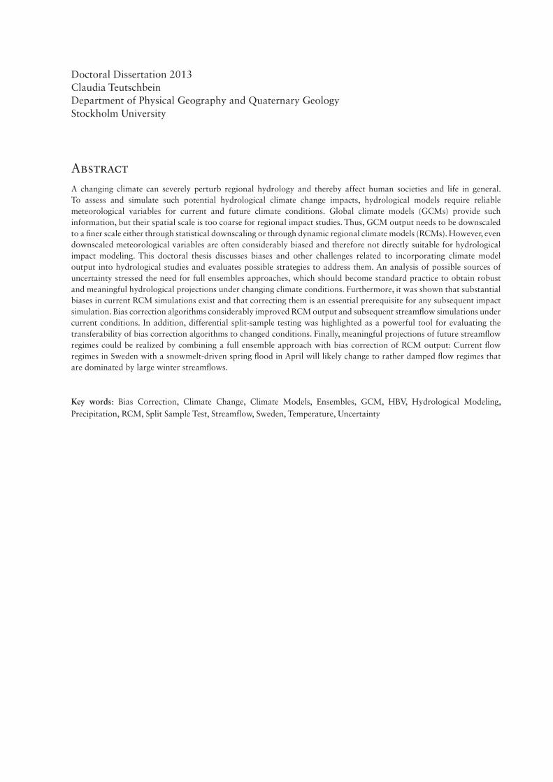
AbstractA changing climate can severely perturb regional hydrology and thereby affect human societies and life in general. To assess and simulate such potential hydrological climate change impacts, hydrological models require reliable meteorological variables for current and future climate conditions. Global climate models (GCMs) provide such information, but their spatial scale is too coarse for regional impact studies. Thus, GCM output needs to be downscaled to a finer scale either through statistical downscaling or through dynamic regional climate models (RCMs). However, even downscaled meteorological variables are often considerably biased and therefore not directly suitable for hydrological impact modeling. This doctoral thesis discusses biases and other challenges related to incorporating climate model output into hydrological studies and evaluates possible strategies to address them. An analysis of possible sources of uncertainty stressed the need for full ensembles approaches, which should become standard practice to obtain robust and meaningful hydrological projections under changing climate conditions. Furthermore, it was shown that substantial biases in current RCM simulations exist and that correcting them is an essential prerequisite for any subsequent impact simulation. Bias correction algorithms considerably improved RCM output and subsequent streamflow simulations under current conditions. In addition, differential split-sample testing was highlighted as a powerful tool for evaluating the transferability of bias correction algorithms to changed conditions. Finally, meaningful projections of future streamflow regimes could be realized by combining a full ensemble approach with bias correction of RCM output: Current flow regimes in Sweden with a snowmelt-driven spring flood in April will likely change to rather damped flow regimes that are dominated by large winter streamflows.

Key words: Bias Correction, Climate Change, Climate Models, Ensembles, GCM, HBV, Hydrological Modeling, Precipitation, RCM, Split Sample Test, Streamflow, Sweden, Temperature, Uncertainty

I saw the alchemy of perspective reduce my world, and all my other life, to grains in a cup.

I learned to watch, to put my trust in other hands than mine. And I learned to wander.

I learned what every dreaming child needs to know - that no horizon is so far that you

cannot get above it or beyond it.

These I learned at once.

But most things came harder.

Beryl Markham(the first women to fly solo across

the Atlantic from east to west)

“

“

List of Papers

This doctoral thesis consists of a summary and four papers. The papers are referred to as Papers I-IV in the summary text.

I. Teutschbein, C., Wetterhall, F. and Seibert, J. (2011). Evaluation of Different Downscaling Techniques for Hydrological Climate-Change Impact Studies at the Catchment Scale. Climate Dynamics, vol. 37(9-10), pages 2087-2105, doi:10.1007/s00382-010-0979-8.

Reprinted with kind permission from Springer Science and Business Media.

II. Teutschbein, C. and Seibert, J. (2010). Regional Climate Models for Hydrological Impact Studies at the Catchment Scale: A Review of Recent Modeling Strategies. Geography Compass, vol. 4(7), pages 834-860. doi: 10.1111/j.1749-8198.2010.00357.x.

Reprinted with kind permission from John Wiley and Sons.

III. Teutschbein, C. and Seibert, J. (2012). Bias correction of regional climate model simulations for hydrological climate-change impact studies: Review and evaluation of different methods, Journal of Hydrology, vol. 456–457, pages 12-29, doi:10.1016/j.jhydrol.2012.05.052.

Reprinted with kind permission from Elsevier.

IV. Teutschbein, C. and Seibert, J. (2012). Is bias correction of Regional Climate Model (RCM) simulations possible for non-stationary conditions? Hydrology and Earth System Sciences Discussions, vol. 9(11), pages 12765-12795, doi: 10.5194/hessd-9-12765-2012. In review.

Co-Authorship

I led the writing of all four papers, was responsible for setting up the hydrological model, carried out the streamflow simulations and interpreted the results.

For paper I, I produced the hydrological results presented in the paper. Fredrik Wetterhall provided climate model data and was responsible for the statistical downscaling of precipitation. Jan Seibert participated in the simulation series design and result interpretation. The final formulation of the paper is a result of collaboration between all authors.

For papers II, III and IV, I gathered relevant catchment information, mathematical information about different bias correction methods as well as climate model data. It was my responsibility to implement the required programming and apply the bias correction procedures. I performed all hydrological simulations. Jan Seibert contributed in the interpretation of the results and formulation of the papers.


Transferring Large-Scale Information from Global Climate Models to the Catchment Scale

Claudia Teutschbein

Contents

1 Introduction . . . . . . . . . . . . . . . . . . . . . . . . . . . . . . . . . . . . . . . . . . . . . . . . . . . . . . . 9

1.1 Climate Change and Hydrology ....................................................................................................9

1.2 Downscaling Climate Models from Global to Catchment Scale ...................................................9

1.2.1 Statistical Downscaling ...................................................................................................................... 9

1.2.2 Dynamical Downscaling .................................................................................................................. 10

1.3 Bias Correction of Downscaled Climate Model Data ..................................................................12

1.3.1 Background on Bias Correction ...................................................................................................... 12

1.3.2 Controversy about Bias Correction ................................................................................................. 12

1.4 Hydrological Modeling of Climate Change Impacts....................................................................12

1.5 Uncertainties in the Modeling Chain ...........................................................................................13

2 Thesis Objectives . . . . . . . . . . . . . . . . . . . . . . . . . . . . . . . . . . . . . . . . . . . . . . . . . . 14

2.1 Paper I ........................................................................................................................................14

2.2 Paper II .......................................................................................................................................14

2.3 Paper III ......................................................................................................................................14

2.4 Paper IV ......................................................................................................................................14

3 Methods . . . . . . . . . . . . . . . . . . . . . . . . . . . . . . . . . . . . . . . . . . . . . . . . . . . . . . . . . 15

3.1 Study Areas ................................................................................................................................15

3.1.1 Storbäcken/Ostträsket ...................................................................................................................... 15

3.1.2 Tännån/Tännfors/Tänndalen ............................................................................................................ 15

3.1.3 Vattholmaån/Fyrisån ........................................................................................................................ 16

3.1.4 Brusaån/Brusafors ............................................................................................................................ 16

3.1.5 Rönne Å ........................................................................................................................................... 16

3.2 Design of the Modeling Chain ....................................................................................................16

3.3 Observed Climate Data ...............................................................................................................17

3.4 Simulated Climate Data and Post-Processing ..............................................................................17

3.4.1 Paper I: Statistical Downscaling ...................................................................................................... 17

3.4.2 Paper II: Dynamical Downscaling .................................................................................................... 17

3.4.3 Paper III: Bias Correction ................................................................................................................ 18

3.4.4 Paper IV: Bias Correction and Differential Split-Sample Testing ....................................................... 18

3.5 Hydrological Model ....................................................................................................................21

3.6 Analysis of Results ......................................................................................................................21

4 Results . . . . . . . . . . . . . . . . . . . . . . . . . . . . . . . . . . . . . . . . . . . . . . . . . . . . . . . . . . 22

4.1 Paper I: Statistical Downscaling ..................................................................................................22

4.1.1 Current and Future Simulations of Precipitation .............................................................................. 22

4.1.2 Projections of Future Streamflow ..................................................................................................... 22

4.2 Paper II: Dynamical Downscaling ...............................................................................................23

4.2.1 Recent Modeling Strategies .............................................................................................................. 23

4.2.2 Streamflow Simulations with Uncorrected RCM Data for Current Climate Conditions ................... 24

4.3 Paper III: Bias Correction ............................................................................................................24

4.3.1 Bias Correction of Precipitation ....................................................................................................... 24

4.3.2 Bias Correction of Temperature ....................................................................................................... 25

4.3.3 Performance Ranking of Bias Correction Methods .......................................................................... 25

4.3.4 Streamflow Simulations with Bias-Corrected RCM Data ................................................................. 25

4.3.5 Impact of Different Variability Sources on Streamflow Characteristics ............................................. 27

4.3.6 Evaluation of Bias Correction Methods according to their Hydrological Performance .................... 28

4.4 Paper IV: Bias Correction and Differential Split-Sample Testing ..................................................30

4.4.1 Relative Errors of Annual Values ..................................................................................................... 30

4.4.2 Ability of Bias Correction Methods to Reproduce Statistical Properties during Validation Period .... 30

5 Discussion . . . . . . . . . . . . . . . . . . . . . . . . . . . . . . . . . . . . . . . . . . . . . . . . . . . . . . . . 33

5.1 Climate Change and Hydrology ..................................................................................................33

5.2 Downscaling Climate Models from Global to Catchment Scale ..................................................33

5.2.1 Choice of Downscaling Method ....................................................................................................... 33

5.2.2 Statistical Downscaling .................................................................................................................... 33

5.2.3 Dynamical Downscaling .................................................................................................................. 33

5.3 Bias Correction of Downscaled Climate Model Data ..................................................................34

5.4 Hydrological Modeling of Climate-Change Impacts ...................................................................36

5.5 Uncertainties in the Modeling Chain ...........................................................................................36

6 Conclusions . . . . . . . . . . . . . . . . . . . . . . . . . . . . . . . . . . . . . . . . . . . . . . . . . . . . . . 37

7 Future Research . . . . . . . . . . . . . . . . . . . . . . . . . . . . . . . . . . . . . . . . . . . . . . . . . . . 38

8 References . . . . . . . . . . . . . . . . . . . . . . . . . . . . . . . . . . . . . . . . . . . . . . . . . . . . . . . . 38

9 Acknowledgements . . . . . . . . . . . . . . . . . . . . . . . . . . . . . . . . . . . . . . . . . . . . . . . . . 44

10 Financial Support . . . . . . . . . . . . . . . . . . . . . . . . . . . . . . . . . . . . . . . . . . . . . . . . . . 44

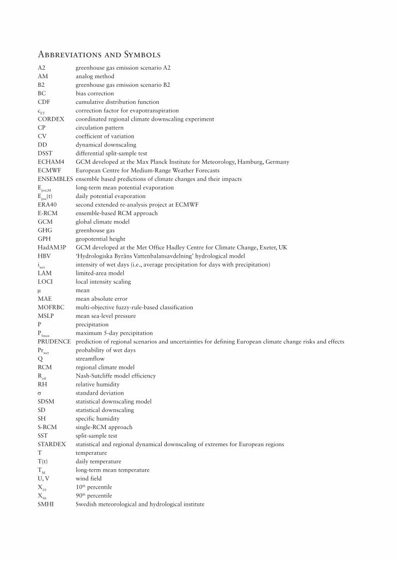
Abbreviations and SymbolsA2 greenhouse gas emission scenario A2AM analog method B2 greenhouse gas emission scenario B2 BC bias correctionCDF cumulative distribution function cET correction factor for evapotranspiration CORDEX coordinated regional climate downscaling experimentCP circulation patternCV coefficient of variation DD dynamical downscaling DSST differential split-sample test ECHAM4 GCM developed at the Max Planck Institute for Meteorology, Hamburg, Germany ECMWF European Centre for Medium-Range Weather ForecastsENSEMBLES ensemble based predictions of climate changes and their impacts Epot,M long-term mean potential evaporation Epot(t) daily potential evaporation ERA40 second extended re-analysis project at ECMWFE-RCM ensemble-based RCM approach GCM global climate model GHG greenhouse gas GPH geopotential heightHadAM3P GCM developed at the Met Office Hadley Centre for Climate Change, Exeter, UK HBV ‘Hydrologiska Byråns Vattenbalansavdelning’ hydrological modeliwet intensity of wet days (i.e., average precipitation for days with precipitation) LAM limited-area model LOCI local intensity scalingm mean MAE mean absolute error MOFRBC multi-objective fuzzy-rule-based classification MSLP mean sea-level pressureP precipitation P5max maximum 5-day percipitation PRUDENCE prediction of regional scenarios and uncertainties for defining European climate change risks and effectsPrwet probability of wet days Q streamflow RCM regional climate modelReff Nash-Sutcliffe model efficiencyRH relative humidity s standard deviation SDSM statistical downscaling model SD statistical downscaling SH specific humidityS-RCM single-RCM approach SST split-sample test STARDEX statistical and regional dynamical downscaling of extremes for European regionsT temperature T(t) daily temperature TM long-term mean temperature U, V wind fieldX10 10th percentile X90 90th percentile SMHI Swedish meteorological and hydrological institute


9

1 IntroductIon

1.1 Climate Change and Hydrology

Water is an essential resource for all forms of life on our planet. Substantial effects of a changing climate are mediated through changes in the water cycle, because water resources are very sensitive to changing climate conditions. Thus, hydrological impacts of changing climate conditions are a potential threat to human societies as they often have serious consequences for agriculture, people living near water bodies, hydropower production and ecosystems. Therefore, it is necessary to provide information on potential future changes in the hydrological cycle to enable decision makers to develop possible mitigation and adaptation strategies.

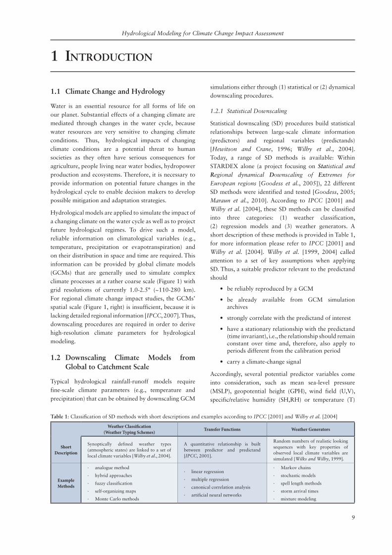
Hydrological models are applied to simulate the impact of a changing climate on the water cycle as well as to project future hydrological regimes. To drive such a model, reliable information on climatological variables (e.g., temperature, precipitation or evapotranspiration) and on their distribution in space and time are required. This information can be provided by global climate models (GCMs) that are generally used to simulate complex climate processes at a rather coarse scale (Figure 1) with grid resolutions of currently 1.0-2.5° (~110-280 km). For regional climate change impact studies, the GCMs’ spatial scale (Figure 1, right) is insufficient, because it is lacking detailed regional information [IPCC, 2007]. Thus, downscaling procedures are required in order to derive high-resolution climate parameters for hydrological modeling.

1.2 Downscaling Climate Models from Global to Catchment Scale

Typical hydrological rainfall-runoff models require fine-scale climate parameters (e.g., temperature and precipitation) that can be obtained by downscaling GCM

simulations either through (1) statistical or (2) dynamical downscaling procedures.

1.2.1 Statistical Downscaling

Statistical downscaling (SD) procedures build statistical relationships between large-scale climate information (predictors) and regional variables (predictands) [Hewitson and Crane, 1996; Wilby et al., 2004]. Today, a range of SD methods is available: Within STARDEX alone (a project focusing on Statistical and

Regional dynamical Downscaling of Extremes for

European regions [Goodess et al., 2005]), 22 different SD methods were identified and tested [Goodess, 2005; Maraun et al., 2010]. According to IPCC [2001] and Wilby et al. [2004], these SD methods can be classified into three categories: (1) weather classification, (2) regression models and (3) weather generators. A short description of these methods is provided in Table 1, for more information please refer to IPCC [2001] and Wilby et al. [2004]. Wilby et al. [1999, 2004] called attention to a set of key assumptions when applying SD. Thus, a suitable predictor relevant to the predictand should

• be reliably reproduced by a GCM

• be already available from GCM simulation archives

• strongly correlate with the predictand of interest

• have a stationary relationship with the predictand (time invariant), i.e., the relationship should remain constant over time and, therefore, also apply to periods different from the calibration period

• carry a climate-change signal

Accordingly, several potential predictor variables come into consideration, such as mean sea-level pressure (MSLP), geopotential height (GPH), wind field (U,V), specific/relative humidity (SH,RH) or temperature (T)

Weather Classification (Weather Typing Schemes) Transfer Functions Weather Generators

ShortDescription

Synoptically defined weather types (atmospheric states) are linked to a set of local climate variables [Wilby et al., 2004].

A quantitative relationship is built between predictor and predictand [IPCC, 2001].

Random numbers of realistic looking sequences with key properties of observed local climate variables are simulated [Wilks and Wilby, 1999].

ExampleMethods

∙ analogue method

∙ hybrid approaches

∙ fuzzy classification

∙ self-organizing maps

∙ Monte Carlo methods

∙ linear regression

∙ multiple regression

∙ canonical correlation analysis

∙ artificial neural networks

∙ Markov chains

∙ stochastic models

∙ spell length methods

∙ storm arrival times

∙ mixture modeling

Table 1: Classification of SD methods with short descriptions and examples according to IPCC [2001] and Wilby et al. [2004]

Claudia Teutschbein

10

[Wilby et al., 2004]. The choice of predictors and SD methods to downscale precipitation time series has a major impact on subsequent modeling procedures and needs to be carefully assessed [Wilby et al., 2002; Teutschbein et al., 2011].

Wilby et al. [2002] described SD as computationally cheap and flexible, which makes it attractive for climate impact studies [Goodess et al., 2012]. It facilitates uncertainty analyses, but the reliability of projections depends strongly on the quality of calibration data, the choice of predictor and the selected SD scheme. The main caveat of SD is the assumption that the derived relationships are also valid in a future perturbed climate.

1.2.2 Dynamical Downscaling

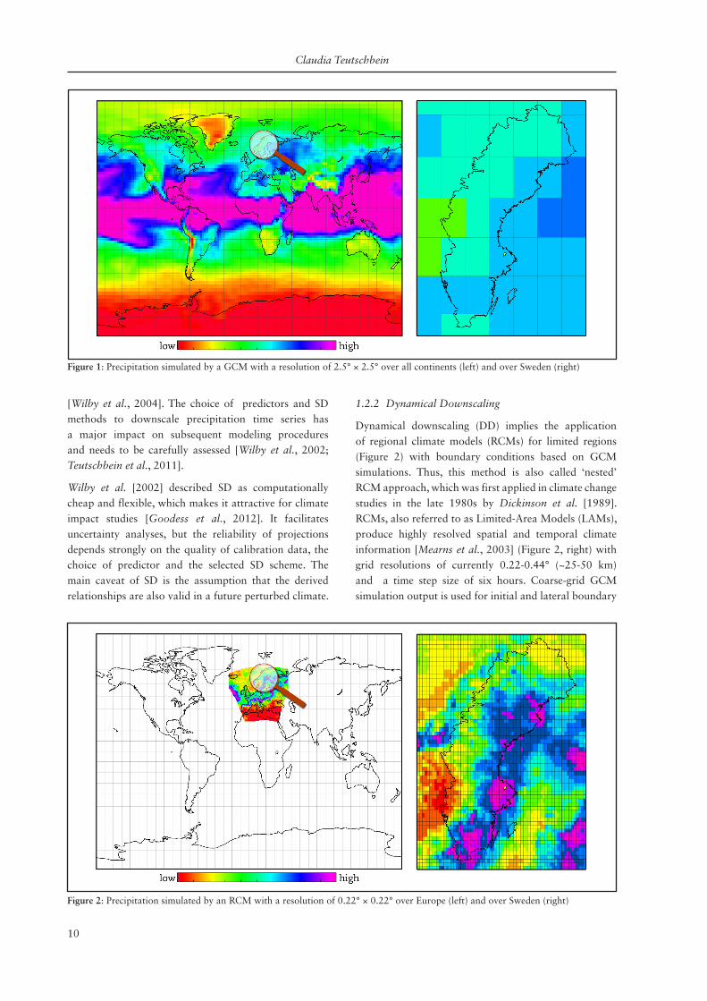
Dynamical downscaling (DD) implies the application of regional climate models (RCMs) for limited regions (Figure 2) with boundary conditions based on GCM simulations. Thus, this method is also called ‘nested’ RCM approach, which was first applied in climate change studies in the late 1980s by Dickinson et al. [1989]. RCMs, also referred to as Limited-Area Models (LAMs), produce highly resolved spatial and temporal climate information [Mearns et al., 2003] (Figure 2, right) with grid resolutions of currently 0.22-0.44° (~25-50 km) and a time step size of six hours. Coarse-grid GCM simulation output is used for initial and lateral boundary

Figure 1: Precipitation simulated by a GCM with a resolution of 2.5° × 2.5° over all continents (left) and over Sweden (right)

Figure 2: Precipitation simulated by an RCM with a resolution of 0.22° × 0.22° over Europe (left) and over Sweden (right)


11

conditions, which is called a ‘one-way nesting approach’ [Mearns et al., 2003]. Although the one-way mode (without feedback from RCM to GCM) is implemented in most RCM studies, two-way nesting with feedback from RCM simulations back to the GCM is a possible alternative [Lorenz and Jacob, 2005; Foley, 2010; Bowden et al., 2011; Chan et al., 2012].

DD is able to resolve atmospheric processes, guarantees consistency with the driving GCM and generates internally consistent output variables [Wilby et al., 2002]. The main drawbacks are the requirement of powerful computing capacities and the dependency on initial and boundary conditions. There is also still a lack of readily available climate scenario ensembles for most regions in the world, although the number of publically available ensemble archives from European projects on similar grid size is increasing, e.g., CORDEX [Evans, 2011], ENSEMBLES [Van der Linden and Mitchell, 2009] and PRUDENCE [Christensen et al., 2007].

Even though most RCM simulations also include certain hydrological components such as surface and subsurface runoff, these simulations do not often agree with streamflow observations (Figure 3) [Teutschbein and Seibert, 2010]. Thus, RCM-simulated hydrological variables might not be directly useful for hydrological impact studies at the catchment scale [Bergström et al., 2001; Graham et al., 2007a, 2007b]. Consequently, other RCM-simulated variables such as temperature and precipitation are most commonly used in an offline mode as input to hydrological models. However, even RCM simulations of temperature and precipitation are often considerably biased [Varis et al., 2004; Christensen et al., 2008; Teutschbein and Seibert, 2010] and should be handled with caution. Typical examples for such biases are the occurrence of too many wet days with low-intensity precipitation or the inaccurate estimation of extreme temperatures [Ines and Hansen, 2006]. Other even more problematic biases can include general under- and overestimation or incorrect simulations of seasonal precipitation pattern [Christensen et al., 2008; Terink et al., 2009; Teutschbein and Seibert, 2010]. The reasons for systematic biases include imperfect model conceptualization, discretization and spatial averaging within grid cells. This poses an obstacle for using RCM simulations as direct driving forces for hydrological impact studies. One possible approach to address this problem is the application of several RCMs [Giorgi, 2006; Déqué et al., 2007; Teutschbein and Seibert, 2010; Ehret et al., 2012] as this often leads to a wide spectrum of different simulation results, that are often referred to as ‘ensemble simulations’. Multi-model approaches (i.e., ensembles) have two advantages: (1) the spread

Figure 3: Long-term seasonal surface runoff (1961-1990) as simulated by a set of ERA40-driven RCMs (gray dashed lines) for the Vattholmaån catchment in southeastern Sweden. Observations (black circles) and the RCM-ensemble mean (gray continuous line) are displayed as well.

Figure 4: Monthly mean temperature and total monthly precipitation for the period 1961-1990 as simulated by individual RCMs (gray dashed lines) for the Vattholmaån catchment in southeastern Sweden. Observations (black circles) and the RCM-ensemble means (gray continuous line) are displayed as well.

Claudia Teutschbein

12

of individual ensemble members covers a more realistic range of uncertainty and (2) the ensemble median may fit observations better [Teutschbein and Seibert, 2010], which is especially true for temperature simulations (Figure 4, top). For precipitation simulations, however, even the ensemble median often deviates from observations and is not able to capture the variability in the observations (Figure 4, bottom). This demonstrates that the implementation of ensemble projections is not sufficient and that further measures, such as bias correction, are needed.

1.3 Bias Correction of Downscaled Climate Model Data

1.3.1 Background on Bias Correction

The term ‘bias correction’ describes the process of re-scaling climate model output to reduce the effects of systematic errors in the climate models [Teutschbein and Seibert, 2010]. Please note that ‘bias correction’ refers exclusively to post-processing RCM output in the context of this thesis and the attached papers.

The underlying idea of bias correction is the identification of possible biases between observed and simulated climate variables, which is the basis for correcting both control and scenario RCM runs with a transformation algorithm. In fact, most bias correction methods are by their nature a form of statistical downscaling which was originally designed to downscale GCM runs. Several bias correction approaches have been developed to downscale climate variables from climate models [Chen et al., 2011a, 2011b; Johnson and Sharma, 2011]. They can be classified according to their degree of complexity and include simple-to-apply methods such as scaling factors but also more sophisticated methods such as probability mapping. Although bias correction of RCM climate variables considerably improves hydrological simulations [Teutschbein and Seibert, 2012a], there is a major drawback: all bias correction methods follow the assumption of stationary model errors [Maraun, 2012; Teutschbein and Seibert, 2012b]. This implies that the correction algorithm and its parameterization for current climate conditions are assumed to also be valid under the conditions of a changed future climate.

1.3.2 Controversy about Bias Correction

Bias correction is a controversial subject that is caught in crossfire more and more often (e.g., Ehret et al. [2012]). Despite their advantageous ability to reduce biases in climate model output, the main concerns raised are that:

• physical causes of model biases are not taken into account and, thus, a proper physical foundation is missing [Teutschbein and Seibert, 2012a]

• spatiotemporal field consistency and relations between climate variables are modified [Ehret et al., 2012]

• conservation principles are not met [Ehret et al., 2012]

• feedback mechanisms are neglected [Ehret et al., 2012]

• the stationarity (time invariance) assumption is likely not met under changing climate conditions [Teutschbein and Seibert, 2012a]

• variability ranges might be reduced without physical justification [Ehret et al., 2012]

• the climate-change signal might be altered [Hagemann et al., 2011; Dosio et al., 2012]

• the choice of bias correction technique is an additional source of uncertainty [Chen et al., 2011b; Teutschbein et al., 2011; Teutschbein and Seibert, 2012a]

• the added value of bias correction is questionable in a complex modeling chain with other major sources of uncertainty [Muerth et al., 2012]

• impacts of bias corrections and related uncertainties are often not communicated to end-users [Ehret et al., 2012]

Therefore, bias correction methods are often criticized to diminish the advantages of climate models. As of the time of writing this thesis, however, no obvious method has been established to replace bias correction and solve all issues listed above. Potential suggestions include ensemble projections and improved climate models, e.g., enhanced process descriptions and increased spatial resolutions [Maraun et al., 2010; Teutschbein and Seibert, 2010, 2012a; Ehret et al., 2012].

1.4 Hydrological Modeling of Climate Change Impacts

Computer-based models to simulate hydrological regimes were relatively rare until the 1960’s. In the following years, however, the number of different conceptual, lumped and more physically-based distributed models that were developed and programmed on computers increased dramatically. Parallel to the development of computer technology, hydrological models improved continually. Nowadays, the application of complicated models at higher resolutions is possible in much shorter time than in the past. Aside from the technological development, hydrology as a scientific discipline has opened up throughout the years and has become more interdisciplinary. It is intrinsically tied to other scientific


13

areas such as climate change science. Today we know that changes in the climate, for instance caused by variations in the chemical composition of the atmosphere, have direct and indirect impacts on the hydrological cycle. Vice versa, modifications in the hydrological cycle can affect local [Lobell et al., 2009; Jarsjö et al., 2012] and global climate [Foley et al., 2003; Puma and Cook, 2010]. Despite the obvious connection, coupling hydrology and climate science together is a relatively young discipline. Due to an increasing awareness regarding climate change amongst the public and the research community, questions arose such as ’What will happen to our Earth’s water resources in the future?’. Thus, the demand for simulations of potential hydrological changes under future climate conditions has increased in recent years.

Researchers have studied climate change effects on runoff in general [Bergström et al., 2001], on flood frequencies [Cameron, 2006], on groundwater levels [Goderniaux et al., 2009], soil moisture [Mavromatis, 2012], water quality [Wilby et al., 2006] and evaporation [Kay and Davies, 2008]. However, most of the available hydrological studies focus either on climate change impacts at a relatively large spatial scale or on projections at a low temporal resolution (seasonal/annual changes etc.). In contrast, the number of studies on regional impacts or extreme events, such as flooding peaks and droughts, is limited.

The current lack of scientifically-approved standard procedures to post-process climate model outputs for subsequent (hydrological) impact analyses is a fundamental problem. Furthermore, the uncertainty in resulting hydrological simulations has yet not been fully evaluated also because limited computer power is partly impeding further investigations.

1.5 Uncertainties in the Modeling Chain

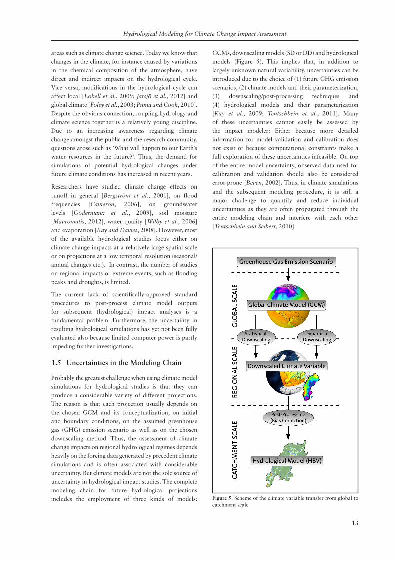
Probably the greatest challenge when using climate model simulations for hydrological studies is that they can produce a considerable variety of different projections. The reason is that each projection usually depends on the chosen GCM and its conceptualization, on initial and boundary conditions, on the assumed greenhouse gas (GHG) emission scenario as well as on the chosen downscaling method. Thus, the assessment of climate change impacts on regional hydrological regimes depends heavily on the forcing data generated by precedent climate simulations and is often associated with considerable uncertainty. But climate models are not the sole source of uncertainty in hydrological impact studies. The complete modeling chain for future hydrological projections includes the employment of three kinds of models:

GCMs, downscaling models (SD or DD) and hydrological models (Figure 5). This implies that, in addition to largely unknown natural variability, uncertainties can be introduced due to the choice of (1) future GHG emission scenarios, (2) climate models and their parameterization, (3) downscaling/post-processing techniques and (4) hydrological models and their parameterization [Kay et al., 2009; Teutschbein et al., 2011]. Many of these uncertainties cannot easily be assessed by the impact modeler: Either because more detailed information for model validation and calibration does not exist or because computational constraints make a full exploration of these uncertainties infeasible. On top of the entire model uncertainty, observed data used for calibration and validation should also be considered error-prone [Beven, 2002]. Thus, in climate simulations and the subsequent modeling procedure, it is still a major challenge to quantify and reduce individual uncertainties as they are often propagated through the entire modeling chain and interfere with each other [Teutschbein and Seibert, 2010].

Figure 5: Scheme of the climate variable transfer from global to catchment scale

Claudia Teutschbein

14

2 thesIs objectIves

Although both GCMs and RCMs have been frequently used in recent years to provide hydrologists with climate variables, linking climate model output to hydrological models is still a relatively new field of research. Coherent scientific standards have not yet been established and there is no ‘common practice’ in terms of how to best apply climate model simulations for impact studies. Furthermore, the quality of climate model output and potential post-processing methods is still a much debated subject amongst climate modelers. In particular the associated uncertainties continue to pose a challenge for impact analyses. Although researchers are now aware of uncertainties introduced in the modeling chain, it is still difficult to handle, decrease and interpret them in a proper way. Therefore, the focus of this thesis is on the assessment of climate change impacts on regional hydrology with special consideration of uncertainties and their propagation into hydrological simulations. The aim was to evaluate different modeling strategies, i.e., ways of transferring large-scale information from climate models to the catchment scale for hydrological climate change impact studies. This general aim served as guiding theme for the four publications included in this thesis that are shortly summarized hereafter.

2.1 Paper I

Teutschbein, C., Wetterhall, F. and Seibert, J. (2011). Evaluation of Different Downscaling Techniques for Hydrological Climate-Change Impact Studies at the Catchment Scale. Climate Dynamics, vol. 37(9-10), pages 2087-2105, doi:10.1007/s00382-010-0979-8.

This paper investigates the influence of different SD approaches on streamflow simulations. Three SD methods were tested to downscale precipitation from two GCMs. The obtained higher-resolution precipitation was then used to simulate streamflow for current (1961-1990) and future (2071-2100) climate conditions with the hydrological model HBV.

2.2 Paper II

Teutschbein, C. and Seibert, J. (2010). Regional Climate Models for Hydrological Impact Studies at the Catchment Scale: A Review of Recent Modeling Strategies. Geography Compass, vol. 4(7), pages 834-860. doi: 10.1111/j.1749-8198.2010.00357.x

This article presents a literature review of potential modeling strategies for applying RCM output in hydrological impact studies. Based on a case study using control-run simulations of 14 different RCMs, the biases of and the variability between different RCMs are highlighted. The paper further gives a short overview of possible bias-correction methods and shows that inter-RCM variability also has substantial consequences for hydrological impact studies in addition to other sources of uncertainties in the modeling chain.

2.3 Paper III

Teutschbein, C. and Seibert, J. (2012). Bias correction of regional climate model simulations for hydrological climate-change impact studies: Review and evaluation of different methods, Journal of Hydrology, vol. 456–457, pages 12-29, doi:10.1016/j.jhydrol.2012.05.052.

This paper provides a summary of available bias correction methods and demonstrates how they can be used to correct deviations in an ensemble of 11 different RCM-simulated temperature and precipitation series. The post-processed climate data was compared to observed climate data. Furthermore, the combined influence of bias-corrected RCM-simulated temperature and precipitation on hydrological simulations was analyzed under current (1961–1990) and future (2021-2050) climate conditions.

2.4 Paper IV

Teutschbein, C. and Seibert, J. (2012). Is bias correction of Regional Climate Model (RCM) simulations possible for non-stationary conditions? Hydrology and Earth System Sciences Discussions, vol. 9(11), pages 12765-12795, doi: 10.5194/hessd-9-12765-2012. In review.

The main concern of bias correction procedures is the underlying assumption that RCM biases are stationary and do not change over time. Accordingly, correction algorithms and parameters derived for current climate conditions are assumed to also apply to future climate conditions. As observations of future conditions are, by their nature, not available in present, it is impossible to verify this assumption. This study, however, demonstrates how differential split-sample testing can be used to evaluate the reliability of bias correction methods for systematically varying climate conditions.


15

3 Methods

3.1 Study Areas

Climate change impacts on regional hydrology were assessed for different climatic conditions and land-use types. Suitable catchments were required to be relatively small, predominantly unregulated and with a spatially rather uniform land-cover. Continuous temperature, precipitation and streamflow measurements needed to be available for the period 1961-1990. Papers II-IV are therefore based on five Swedish catchments with areas from 147 to 293 km2 (Figure 6), which are further described below. Please note that Paper I is based on one catchment, the Vattholmaån river basin (catchment 3, described below).

3.1.1 Storbäcken/Ostträsket

The catchment of river Storbäcken is located farthest north of all sites (station Ostträsket #50127: N64.9°, E21.1°). The climate in this area is continental subarctic with an annual mean temperature of 2.1°C and a total precipitation of 617 mm per year. The catchment has an area of 150 km2. It is dominated by forest (79%) with small portions of open land (9%) and lakes/wetlands (12%).

3.1.2 Tännån/Tännfors/Tänndalen

River Tännån is situated in a mountainous area in the western part of central Sweden (station Tänndalen #1223: N62.5°, E12.3°). The region has a continental

Figure 6: Map showing locations and land-use types of the Swedish study areas. The grid indicates the spatially interpolated 4×4 km national grid of observed precipitation and temperature. Catchments: (1) Tännfors, (2) Storbäcken, (3) Vattholmaån, (4) Brusaån and (5) Rönne Å.

Claudia Teutschbein

16

subarctic climate with a tendency towards polar tundra climate. The annual mean temperature is -0.5°C and total annual precipitation amounts to 775 mm. The catchment has a total area of 227 km2 and is characterized by large parts of alpine tundra. The main types of land-use are open land (60%), forest (32%) and lakes/wetlands (8%).

3.1.3 Vattholmaån/Fyrisån

The catchment of Vattholmaån in southeastern Sweden (station Vattholma #50110: N60.0°, E17.7°) is a subcatchment of river Fyrisån with streamflow records available as from 1916. It is located in a warm summer continental climate zone with an average annual temperature of 5.2°C and a total annual precipitation of 633 mm. It is the largest catchment in this study with an area of 293 km2, which consists of forest (81%), lakes/wetlands (10%), open land (7%) and residential areas (2%).

3.1.4 Brusaån/Brusafors

River Brusaån is located in southern Sweden (station Brusafors #1622: N57.6°, E15.6°) and has an area of 240 km2. The climate in this region is warm summer continental tending towards maritime temperate. The annual mean temperature is 5.7°C with a total precipitation of 632 mm per year. The catchment includes

a large fraction of forested areas (83%), some open land (12%), lakes/wetlands (3%) and residential areas (2%).

3.1.5 Rönne Å

The catchment of Rönne Å is situated farthest south (station Heåkra #2128: N55.8°, E13.6°). The region is characterized by a maritime temperate climate with an annual mean temperature of 7.3°C and a total annual precipitation of 786 mm. With a total area of 147 km2, this catchment is the smallest included in this study. It consists of open land (46%), lakes/wetlands (27%), forested areas (23%) and residential areas (4%).

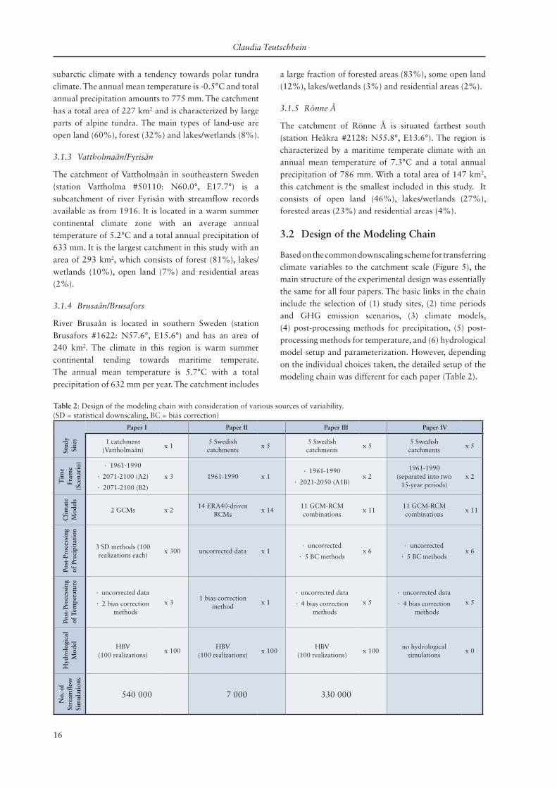
3.2 Design of the Modeling Chain

Based on the common downscaling scheme for transferring climate variables to the catchment scale (Figure 5), the main structure of the experimental design was essentially the same for all four papers. The basic links in the chain include the selection of (1) study sites, (2) time periods and GHG emission scenarios, (3) climate models, (4) post-processing methods for precipitation, (5) post-processing methods for temperature, and (6) hydrological model setup and parameterization. However, depending on the individual choices taken, the detailed setup of the modeling chain was different for each paper (Table 2).

Table 2: Design of the modeling chain with consideration of various sources of variability.(SD = statistical downscaling, BC = bias correction)

Paper I Paper II Paper III Paper IV

Stud

y Si

tes 1 catchment

(Vattholmaån)x 1

5 Swedish catchments

x 55 Swedish catchments

x 55 Swedish catchments

x 5

Tim

e Fr

ame

(Sce

nari

o) ∙ 1961-1990

∙ 2071-2100 (A2)

∙ 2071-2100 (B2)

x 3 1961-1990 x 1 ∙ 1961-1990

∙ 2021-2050 (A1B)x 2

1961-1990 (separated into two

15-year periods)x 2

Clim

ate

Mod

els

2 GCMs x 214 ERA40-driven

RCMsx 14

11 GCM-RCM combinations

x 1111 GCM-RCM combinations

x 11

Post

-Pro

cess

ing

of P

reci

pita

tion

3 SD methods (100 realizations each)

x 300 uncorrected data x 1 ∙ uncorrected

∙ 5 BC methodsx 6

∙ uncorrected

∙ 5 BC methodsx 6

Post

-Pro

cess

ing

of T

empe

ratu

re

∙ uncorrected data

∙ 2 bias correction methods

x 31 bias correction

methodx 1



x 5



x 5

Hyd

rolo

gica

l M

odel HBV

(100 realizations)x 100

HBV(100 realizations)

x 100HBV

(100 realizations)x 100

no hydrological simulations

x 0

No.

of

Stre

amfl

ow

Sim

ulat

ions

540 000 7 000 330 000


17

3.3 Observed Climate Data

Measured daily precipitation, temperature and streamflow series for the control period 1961–1990 were provided by the Swedish Meteorological and Hydrological Institute (SMHI). Observed precipitation and temperature values were obtained from a spatially interpolated 4 x 4 km national grid [Johansson, 2002] (Figure 6) by averaging all grid cells containing parts of the catchment.

3.4 Simulated Climate Data and Post-Processing

3.4.1 Paper I: Statistical Downscaling

The focus of Paper I was on statistical downscaling of precipitation simulated by two GCMs (HadAM3p and ECHAM4) for a control period (1961-1990) and for both GHG emission scenarios A2 and B2 (2071–2100). In order to provide precipitation series, three SD approaches were tested: (1) an analog sorting method (AM) [Lorenz, 1969; Zorita and von Storch, 1999; Obled et al., 2002; Wetterhall et al., 2005], (2) a multi-objective fuzzy-rule-based classification (MOFRBC) [Bardossy and Plate, 1992; Bardossy et al., 1995, 2005; Yang et al., 2010] and (3) a statistical-downscaling model (SDSM) [Wilby et al., 2002].

The AM is conceptually one of the simplest statistical downscaling methods [Zorita and Von Storch, 1999]. The basic assumption is that similar circulation patterns (CPs) should result in similar regional effects [Obled et al., 2002]. Thus, the AM uses historical observations to search for an analog that best resembles the CP (predictors) simulated by the GCM. The corresponding regional observations (predictands) are then linked to the GCM simulations.

MOFRBC is a semi-objective (i.e., fuzzy) CP classification method which can be considered a combination of subjective and objective classification procedures [Özelkan et al., 1998]. Subjective (i.e., manual) classification methods are based on meteorological experience [Bardossy et al., 2005], whereas objective (i.e., automated) approaches rely on mathematical techniques such as hierarchical and correlation methods [Bardossy et al., 1995]. MOFRBC attempts to preserve the positive aspects and eliminate the limitations of both approaches [Bardossy et al., 2005]. MOFRBC is accomplished in two steps: Firstly, fuzzy logic is used to classify large-scale CPs. According to Stehlík and Bardossy [2002], the advantages of this classification method are objectiveness, automation and consideration of precipitation behavior in a certain

region. Secondly, rainfall frequencies and thereafter rainfall amounts are modeled conditioned on the CPs [Bardossy et al., 2001; Wetterhall et al., 2009]. Earlier studies [Wetterhall et al., 2007, 2009] gave proof that MOFRBC can be implemented for Swedish catchments.

The SDSM is an ‘off-the-shelf’ software package that combines stochastic weather generators and regression-based methods [Wilby et al., 2002]: predictands (e.g., precipitation) are modeled linearly conditioned on CPs and atmospheric moisture variables, whereas the variance of downscaled precipitation is stochastically increased to better fit observations. The software runs under the Microsoft Windows operating system and automates all tasks necessary to statistically downscale climate variables: Wilby et al. [2002] summarized that it screens candidate predictor variables, calibrates the model, synthesizes current weather data, generates future climate scenarios and performs diagnostic testing as well as basic statistical analysis. The SDSM has been applied to a number of catchments in China [Wetterhall et al., 2006], Great Britain [Diaz-Nieto and Wilby, 2005; Prudhomme

and Davies, 2009a, 2009b], the United States [Wilby et al., 1999, 2000; Hay et al., 2000] and Sweden [Wetterhall et al., 2007].

In Paper I, 100 stochastically simulated realizations of precipitation were produced for each SD method, with each realization having equal probability. This allowed the assessment of the SD-realization variability in the resulting runoff simulations.

Temperature data was simulated by the same two GCMs (HadAM3P and ECHAM4) for the same periods (1961-1990 and 2071-2100) and the same GHG emission scenarios (A2 and B2). Three different methods of post-processing this temperature data were compared: (1) applying temperature directly as modeled by the GCMs, (2) using the delta-change approach and (3) applying linear scaling (see more details in Table 3).

3.4.2 Paper II: Dynamical Downscaling

The main topic of Paper II was dynamical downscaling: recent applications of RCM output for hydrological impact studies were reviewed. In the presented case study for five Swedish catchments, 14 ERA40-driven RCM simulations of temperature and precipitation for the control period 1961-1990 were obtained from the ENSEMBLES EU project [Van der Linden and Mitchell, 2009] and used as input to the hydrological HBV model. The ERA40 data set is a re-analysis of meteorological observations [Uppala et al., 2005] and resulted from the second extended re-analysis project at the European Centre for Medium-Range Weather Forecasts (ECMWF). Thus,

Claudia Teutschbein

18

all 14 RCMs were driven by the same global data and a direct RCM evaluation could be performed based on their ability to reproduce average and extreme values. Since the objective was to demonstrate the consequences of applying direct RCM output, no bias correction was applied. Initial tests, however, indicated substantial biases in the RCM temperature with profound effects on hydrological simulations. Therefore, a simple linear scaling of temperature was performed to eliminate this source of bias in the hydrological modeling and to allow an assessment of the RCM precipitation simulations.

3.4.3 Paper III: Bias Correction

This paper builds on the work published in Paper II and, thus, also deals with the application of RCM simulations. The aim of Paper III was to analyze how the combined uncertainties of different temperature- and precipitation-bias correction methods might influence subsequent seasonal streamflow and flood peak simulations.

Daily precipitation and temperature series for the periods 1961–1990 (control run) and 2021–2050 (scenario A1B) simulated by 11 RCMs driven by different GCMs (see Paper III) were obtained from the ENSEMBLES project [Van der Linden and Mitchell, 2009]. Due to their relatively small size, the areas of the study catchments were usually only covered by a single RCM grid cell. In Paper II it was found that values of one grid cell do not differ considerably from the average over nine grid cells (i.e., over one grid cell and its eight neighboring cells) for the locations of the five Swedish catchments which are also used in this study. Therefore, RCM precipitation and temperature values were taken from the grid cell with center coordinates closest to the center of the catchment.

In comparison to raw RCM output data (i.e., no correction) the following bias correction methods to adjust RCM simulations were analyzed: (1) linear scaling, (2) local intensity scaling, (3) power transformation, (4) variance scaling, (5) distribution mapping and (6) the delta-change approach. It was also considered to apply a precipitation threshold, which is often used to adjust the wet-day frequencies of precipitation time series. However, since this method does not correct the mean it was not counted as an adequate ‘stand-alone’ bias correction method in our review. Nevertheless, a precipitation threshold was used in combination with other correction approaches to avoid too many drizzle-days as described in more detail in Paper III. All possible combinations of the above mentioned temperature and precipitation correction methods were tested. A short description of all bias correction approaches is given in Table 3. More detailed descriptions were provided in Paper III as well as by Gudmundsson et al. [2012],

Johnson and Sharma [2011] and the original method publications listed in Table 3.

3.4.4 Paper IV: Bias Correction and Differential Split-Sample Testing

Paper IV continues the work published in Paper III with the purpose of testing different bias correction methods under varying climate conditions. The climate data used was the same ENSEMBLES data as in Paper III described above, but only for the period 1961-1990. Furthermore, the study was based on the same bias correction methods for precipitation and temperature as in Paper III. All of these bias correction methods rely on the questionable assumption of stationarity. This is, however, a major limitation which merely has to be made, because we are lacking appropriate methods to deal with changing climate conditions and possible changes in bias relationships. More importantly, it is virtually impossible to test whether the stationarity assumption is true or not. This, however, does not automatically imply that it is also impossible to provide any confidence that the correction algorithms applied to today’s climate are also valid for a future climate. In fact, there is a way to test how well bias correction methods can reproduce conditions different from those that they were calibrated to by using one of the operational testing methods presented by Klemeš [1986]. The hierarchical scheme outlined by Klemeš [1986] includes two approaches of interest for systematic testing of hydrological model transposability: split-sample testing (SST) for stationary conditions and differential split-sample testing (DSST) for non-stationary conditions. SST implies the splitting of an available data record into two (preferably equally sized) segments in order to use one as calibration and one as validation period. DSST on the other hand should, according to Klemeš [1986], be used under changing conditions. The first step of this test includes the identification of two periods with the climate variable of interest having different values, for instance a warm versus a cold or a wet versus a dry period. The model is then calibrated on the period with one condition and validated on the period with the other condition, which allows analyzing the model’s ability to perform under shifting conditions. SST can be equivalent to DSST, if the two segments are by nature characterized by substantially different conditions [Klemeš, 1986].

DSST was applied in this study to test the ability of different bias correction procedures to reliably work under changed climate conditions. Both SST and DSST have hardly been used to evaluate bias correction methods. For instance, Bennett et al. [ 2010] and Terink et al. [ 2010] evaluated bias correction


19

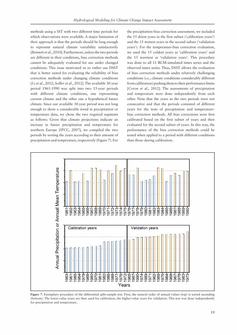
methods using a SST with two different time periods for which observations were available. A major limitation of their approach is that the periods should be long enough to represent natural climate variability satisfactorily [Bennett et al., 2010]. Furthermore, unless the two periods are different in their conditions, bias correction methods cannot be adequately evaluated for use under changed conditions. This issue motivated us to rather use DSST that is better suited for evaluating the reliability of bias correction methods under changing climate conditions [Li et al., 2012; Seiller et al., 2012]. The available 30-year period 1961-1990 was split into two 15-year periods with different climate conditions, one representing current climate and the other one a hypothetical future climate. Since our available 30-year period was not long enough to show a considerable trend in precipitation or temperature data, we chose the two required segments as follows: Given that climate projections indicate an increase in future precipitation and temperature for northern Europe [IPCC, 2007], we compiled the two periods by sorting the years according to their amount of precipitation and temperature, respectively (Figure 7). For

the precipitation-bias correction assessment, we included the 15 driest years in the first subset (’calibration years’) and the 15 wettest years in the second subset (’validation years’). For the temperature-bias correction evaluation, we used the 15 coldest years as ‘calibration years’ and the 15 warmest as ‘validation years’. This procedure was done to all 11 RCM-simulated times series and the observed times series. Thus, DSST allows the evaluation of bias correction methods under relatively challenging conditions (i.e., climate conditions considerably different from calibration) pushing them to their performance limits [Coron et al., 2012]. The assessments of precipitation and temperature were done independently from each other. Note that the years in the two periods were not consecutive and that the periods consisted of different years for the tests of precipitation and temperature-bias correction methods. All bias corrections were first calibrated based on the first subset of years and then evaluated for the second subset of years. In this way, the performance of the bias correction methods could be tested when applied to a period with different conditions than those during calibration.

Figure 7: Exemplary procedure of the differential split-sample test. First, the natural order of annual values (top) is sorted ascending (bottom). The lower-value years are then used for calibration, the higher-value years for validation. This test was done independently for precipitation and temperature.

Claudia Teutschbein

20

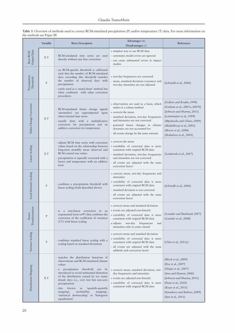
Table 3: Overview of methods used to correct RCM-simulated precipitation (P) and/or temperature (T) data. For more information on the methods see Paper III

Variable Short DescriptionAdvantages (+)

Disadvantages (-)References

Raw

RC

MO

utpu

t D

ata

P, T ∙ RCM-simulated time series are used directly without any bias correction

+ simplest way to use RCM data

- systematic model errors are ignored

- can cause substantial errors in impact studies

Prec

ipit

atio

nT

hres

hold

P

∙ an RCM-specific threshold is calibrated such that the number of RCM-simulated days exceeding this threshold matches the number of observed days with precipitation

∙ rarely used as a ‘stand-alone’ method but often combined with other correction procedures

+ wet-day frequencies are corrected

- mean, standard deviation (variance) and wet-day intensities are not adjusted

[Schmidli et al., 2006]

Del

ta-C

hang

e C

orre

ctio

n

P, T

∙ RCM-simulated future change signals (anomalies) are superimposed upon observational time series

∙ usually done with a multiplicative correction for precipitation and an additive correction for temperature

+ observations are used as a basis, which makes it a robust method

+ corrects the mean

- standard deviation, wet-day frequencies and intensities are not corrected

- potential future changes in climate dynamics are not accounted for

- all events change by the same amount

[Gellens and Roulin, 1998]

[Graham et al., 2007a, 2007b]

[Johnson and Sharma, 2011]

[Lettenmaier et al., 1999]

[Mpelasoka and Chiew, 2009]

[Middelkoop et al., 2001]

[Moore et al., 2008]

[Shabalova et al., 2003]

Lin

ear

Scal

ing

P, T

∙ adjusts RCM time series with correction values based on the relationship between long-term monthly mean observed and RCM control run values

∙ precipitation is typically corrected with a factor and temperature with an additive term

+ corrects the mean

+ variability of corrected data is more consistent with original RCM data

- standard deviation, wet-day frequencies and intensities are not corrected

- all events are adjusted with the same correction factor

[Lenderink et al., 2007]

Loc

al I

nten

sity

Sca

ling

P ∙ combines a precipitation threshold with linear scaling (both described above)

+ corrects mean, wet-day frequencies and intensities


- standard deviation is not corrected

- all events are adjusted with the same correction factor

[Schmidli et al., 2006]

Pow

er

Tra

nsfo

rmat

ion

P

∙ is a non-linear correction in an exponential form (a•Pb) that combines the correction of the coefficient of variation (CV) with linear scaling

+ corrects mean and standard deviation

+ events are adjusted non-linearly


± adjusts wet-day frequencies and intensities only to some extend

[Leander and Buishand, 2007]

[Leander et al., 2008]

Var

ianc

e Sc

alin

g

T ∙ combines standard linear scaling with a scaling based on standard deviations

+ corrects mean and standard deviation


- all events are adjusted with the same addends and correction factor

[Chen et al., 2011a]

Dis

trib

utio

n M

appi

ng

P, T

∙ matches the distribution functions of observations and RCM-simulated climate values

∙ a precipitation threshold can be introduced to avoid substantial distortion of the distribution caused by too many drizzle days (i.e., very low but non-zero precipitation)

∙ also known as ‘quantile-quantile mapping’, ‘probability mapping’, ‘statistical downscaling’ or ‘histogram equalization’

+ corrects mean, standard deviation, wet-day frequencies and intensities

+ events are adjusted non-linearly


[Block et al., 2009]

[Boe et al., 2007]

[Déqué et al., 2007]

[Ines and Hansen, 2006]

[Johnson and Sharma, 2011]

[Piani et al., 2010]

[Rojas et al., 2011]

[Sennikovs and Bethers, 2009]

[Sun et al., 2011]


21

3.5 Hydrological Model

The conceptual rainfall-runoff model HBV [Bergström, 1976] was used to simulate daily streamflow values in Papers I-III (please note that no hydrological simulations were conducted in Paper IV). It employs several different routines that have been implemented to simulate snow, soil moisture, evaporation, groundwater and channel routing, respectively. Further information about HBV can be found in papers on its model structure and parameter uncertainty [Bergström, 1976, 1992; Harlin and Kung, 1992; Lindström et al., 1997; Seibert, 1999]. The HBV model has been applied in various versions in the past. In this study the version HBV-light [Seibert, 2003] was used. HBV-light requires daily temperature, precipitation and potential evaporation values as driving variables. In order to analyze the full spectrum of responses in the modeling chain, several combinations of corrected and uncorrected driving variables were evaluated. Depending on the purpose of a simulation (see Papers I-III), daily temperature and precipitation series simulated by GCMs/RCMs were used either directly or after correction of possible biases (see description of climate data above). Daily potential evaporation Epot(t) (Equation 1) was estimated from long-term mean potential evaporation Epot,M in connection with the difference of daily and long-term mean temperature (T(t)-TM) scaled by a correction factor cET [Lindström et al., 1997].

Epot(t) = (1 + cET ∙ (T(t) - TM)) ∙ Epot,M (1)

with 0 ≤ Epot(t) ≤ 2 ∙ Epot,M

The HBV model was first calibrated to observed streamflow using observed temperature and precipitation series. To account for parameter uncertainty, the model was calibrated 100 times with a genetic algorithm which, due to its stochastic components, resulted in 100 different calibrated parameter sets [Seibert, 2000]. These parameter sets were then used to simulate streamflow using the uncorrected or post-processed GCM/RCM simulations as input.

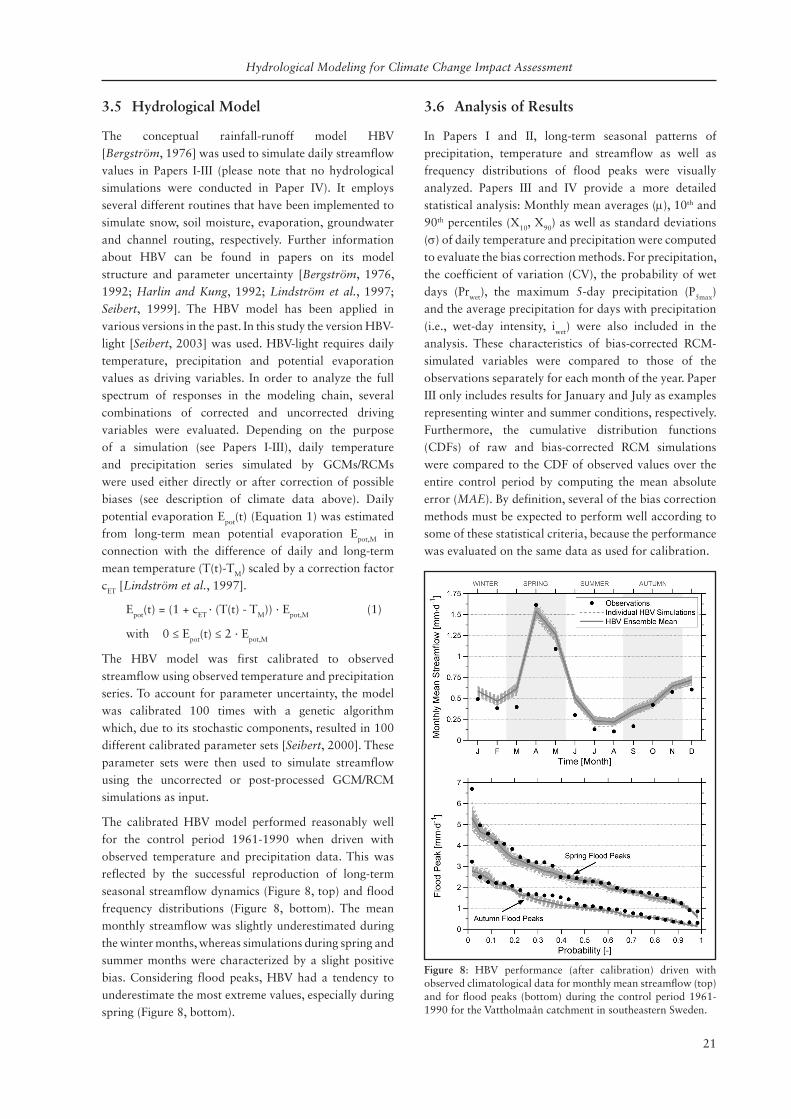
The calibrated HBV model performed reasonably well for the control period 1961-1990 when driven with observed temperature and precipitation data. This was reflected by the successful reproduction of long-term seasonal streamflow dynamics (Figure 8, top) and flood frequency distributions (Figure 8, bottom). The mean monthly streamflow was slightly underestimated during the winter months, whereas simulations during spring and summer months were characterized by a slight positive bias. Considering flood peaks, HBV had a tendency to underestimate the most extreme values, especially during spring (Figure 8, bottom).

3.6 Analysis of Results

In Papers I and II, long-term seasonal patterns of precipitation, temperature and streamflow as well as frequency distributions of flood peaks were visually analyzed. Papers III and IV provide a more detailed statistical analysis: Monthly mean averages (m), 10th and 90th percentiles (X10, X90) as well as standard deviations (s) of daily temperature and precipitation were computed to evaluate the bias correction methods. For precipitation, the coefficient of variation (CV), the probability of wet days (Prwet), the maximum 5-day precipitation (P5max) and the average precipitation for days with precipitation (i.e., wet-day intensity, iwet) were also included in the analysis. These characteristics of bias-corrected RCM-simulated variables were compared to those of the observations separately for each month of the year. Paper III only includes results for January and July as examples representing winter and summer conditions, respectively. Furthermore, the cumulative distribution functions (CDFs) of raw and bias-corrected RCM simulations were compared to the CDF of observed values over the entire control period by computing the mean absolute error (MAE). By definition, several of the bias correction methods must be expected to perform well according to some of these statistical criteria, because the performance was evaluated on the same data as used for calibration.

Figure 8: HBV performance (after calibration) driven with observed climatological data for monthly mean streamflow (top) and for flood peaks (bottom) during the control period 1961-1990 for the Vattholmaån catchment in southeastern Sweden.

Claudia Teutschbein

22

4 results

Detailed results of this doctoral study are presented in the four attached papers. A short summary is given hereafter.

4.1 Paper I: Statistical Downscaling

This paper investigated the influence of three different statistical downscaling (SD) approaches on streamflow simulations for current and future climate conditions.

4.1.1 Current and Future Simulations of Precipitation

Precipitation over the control period 1961-1990 was fairly well simulated with all SD methods in the studied Vattholmaån catchment (Figure 9). However, some variations occurred depending on the applied GCM and SD method: AM was good at capturing the inter-month variability, whereas MOFRBC was characterized by a time lag in monthly precipitation. AM was not able to reproduce the precipitation maximum in July/August, but captured all other months relatively well. MOFRBC and SDSM, on the other hand, were able to capture the magnitude of the precipitation maximum in July/August well, but did not perform as well as AM for all other months. This issue can be seen for downscaled precipitation of both GCMs (Figure 9, left and right). In direct comparison, the ensemble median of 14 uncorrected ERA40-driven RCM simulations had a much smaller inter-month variability and failed to adequately reproduce the annual precipitation maximum.

The variable performances during the control period also re-emerged as strong variability in projected future

precipitation for the period 2071-2100 (Figure 10, top). On average, precipitation was projected to decrease during late summer (July-September), whereas it will likely increase during all other seasons. But these projected changes were highly variable with different combinations of GHG emission scenarios, GCMs and SD methods. The most uncertain month was February with projected precipitation changes of -10.0% to +42.7%. SDSM generally projected a larger range of possible precipitation changes and, thus, was more sensitive to the GCM and scenario choices than AM and MOFRBC.

4.1.2 Projections of Future Streamflow

Simulations of future streamflow resulted in highly variable projections (Figure 10, bottom) that were caused by the choices made in the modeling chain. The choice of emission scenario had the least influence on streamflow simulations, followed by the choice of the GCM. One of the major sources of variability was the choice of SD method for precipitation. Already during the control period it became apparent that the ability of the hydrological model to reproduce observed streamflow was directly related to the skill of each SD method to reproduce observed precipitation. MOFRBC projected an increase of annual streamflow within the range of +2.2% to +11.6%, whereas AM and SDSM projected a decrease within the range of -0.1% to -11.7%.

The streamflow-change signal was projected to flatten out, with more streamflow in winter and less streamflow in spring/summer (Figure 10, bottom). During the colder

Figure 9: Precipitation time series (i.e., median of 100 realizations) downscaled with three statistical downscaling methods (AM, MOFRBC and SDSM) from the two GCMs HadAM3P (top) and ECHAM4 (bottom) during the control period 1961–1990 for the Vattholmaaån catchment. For comparison only, the median of precipitation simulated by 14 ERA40-driven RCMs (not corrected) for the same period is shown as well (gray line).


23

months (i.e., November to March), streamflow was projected to increase considerably up to 90%, whereas most simulations pointed towards a streamflow reduction of -20% to -60% during the warmer months (i.e., April to October). Thus, the current flow regime, which is clearly dominated by a snowmelt-driven spring flood in April (Figure 8, top), will likely change to a rather dampened flow regime with a dominating large winter streamflow.

The complete study was also performed for another nearby catchment of similar size. The results were essentially the same without any major differences.

4.2 Paper II: Dynamical Downscaling

In this article, a literature review of potential modeling strategies for applying RCM output in hydrological impact studies was compiled. Additionally, biases of and the variability between different RCMs were highlighted along with their effects on hydrological streamflow simulations.

4.2.1 Recent Modeling Strategies

To evaluate climate change impacts on hydrology with help of dynamical downscaling (i.e., RCMs), different modeling strategies can be found in the literature, ranging from rather simple systems with only one RCM

- so-called single-RCM investigations (S-RCM) - to more complex ensemble-based RCM studies (E-RCM). The S-RCM approach is often used for analyzing very large watersheds (e.g., Jha et al. [2004], Lee et al. [2004], Payne et al. [2004], Wood et al. [2004], Kleinn et al. [2005] or Kilsby et al. [2007]) or for developing and testing purposes (e.g., Wood et al. [2004], Kay et al. [2006a, 2006b], Bell et al. [2007a, 2007b], Leander and Buishand [2007] or Beldring et al. [2008]). Sometimes also limited computing power, especially in older studies, can be the reason for S-RCM investigations. However, to avoid biased modeling results and to account for inter-model variability, an E-RCM approach is usually more suitable as it relies on more than one RCM and often also on a range of GHG emission scenarios, GCMs and/or hydrological models (e.g., Horton et al. [2006], Bürger et al. [2007], Graham et al.

[2007a] or de Wit et al. [2007]). Studies applying the E-RCM approach are at the time of writing still outnumbered by studies using S-RCM approaches, but their number has continuously increased in recent years which can probably be at least partially related to the parallel enhancement of computing power. Due to the fact that the E-RCM approach accounts for uncertainties introduced at several points in the modeling chain, this approach usually results in the most realistic and trustworthy estimation of uncertainty ranges.

Figure 10: Changes in the annual cycles of precipitation (a) and streamflow (b) in percent as projected by two GCMs (HadAM3P and ECHAM4) downscaled with three different downscaling methods (AM, MOFRBC and SDSM) under the assumption of two GHG emissions scenarios (A2 and B2). Each bar represents the median of 10,000 simulations (100 HBV parameterizations multiplied by 100 downscaling realizations).

Claudia Teutschbein

24

Much of the available literature on dynamical downscaling for hydrological simulations concentrates on catchments in Europe or North-American catchments. Although the list of publications included in the review in Paper II is certainly not complete, this geographical imbalance emphasizes the need for hydrological impact studies based on RCM simulations in other parts of the world where climate change impacts might be different.

4.2.2 Streamflow Simulations with Uncorrected RCM Data for Current Climate Conditions

Uncorrected precipitation and linearly scaled temperature obtained from 14 RCM simulations driven by the same ERA40 re-analysis data were used to simulate streamflow with the HBV-light model for the control period 1961-1990 for five Swedish catchments. The RCMs were to a certain extent only able to provide sufficient data for the streamflow simulations. Although the simulated streamflow hydrograph fitted well with observations in terms of spring and autumn flood peak timing (Figure 11), the long-term mean of peak flows differed considerably (up to ±100%) from observations for several individual RCMs. In general, the ensemble

median fitted observations better than individual RCMs, but there were still large deviations especially for the two southeastern watersheds Vattholmaån and Brusafors.

4.3 Paper III: Bias Correction

This paper showed how bias correction methods could be used to correct deviations in RCM-simulated temperature and precipitation series. Moreover, the combined influence of these bias correction methods on hydrological simulations was analyzed in detail.

4.3.1 Bias Correction of Precipitation

Six approaches for using RCM-simulated precipitation as input for hydrological simulations were evaluated: (1) no correction, (2) linear scaling, (3) local intensity scaling (LOCI), (4) power transformation, (5) distribution mapping and (6) the delta-change approach. These methods are shortly described in Table 3, detailed explanations and mathematical expressions can be found in Paper III. According to the calculated statistical measures, all precipitation-bias corrections were able to improve the raw RCM simulations to some extent.

Figure 11: Long-term averaged (1961-1990) streamflow simulated with HBV forced by 14 different RCMs (gray dashed lines) and forced by observed meteorology (black line). The RCM ensemble median (gray continuous line) and observations (black circles) are shown as well. Note the different scale for the two northernmost catchments (upper row).


25

All methods successfully eliminated the bias in mean daily precipitation. Differences emerged with respect to standard deviation, coefficient of variation and the 90th percentiles of daily precipitation: especially linear scaling and LOCI showed larger variability ranges and still had similarly large biases as uncorrected precipitation series. However, the most substantial discrepancies were related to the occurrence probability of dry days and to the precipitation intensity on wet days. Apart from the delta-change approach, which corresponded to the observations by definition, only LOCI and distribution mapping appropriately adjusted these two statistical measures and reduced the variability between the different RCM simulations. All other methods only partly decreased the variability, but did not succeed in bringing the RCMs closer to observed values.

4.3.2 Bias Correction of Temperature

The following methods for post-processing RCM-simulated temperature were analyzed: (1) no correction, (2) linear scaling, (3) variance scaling, (4) distribution mapping and (5) the delta-change approach. A short description of these approaches can be found in Table 3, for detailed explanations and mathematical expressions please refer to Paper III. All temperature-bias corrections improved the raw RCM simulations according to the statistical performance measures. Unlike for raw RCM temperature, a bias in mean temperature could no longer be found with all correction methods. Based on the performance statistics, most bias correction methods performed equally well. Only the linear-scaling approach stood out as it partly failed to adjust the standard deviation and the 10th/90th percentiles. All other methods considerably improved the raw RCM temperature which also resulted in less variability in the statistical measures. It should be mentioned that the delta-change approach was not included in this statistical analysis, because it coincides with observed values for current conditions by definition, which means that both time series naturally have the same statistics.

4.3.3 Performance Ranking of Bias Correction Methods

Bias correction methods were ranked according to their performance in bringing the RCM median closer to observations (Table 4). Performances were quantified by the mean absolute error (MAE) based on the fit of their CDF with the CDF of observations. The distribution mapping performed best, followed by the power transformation (when applied to precipitation), variance scaling (when applied to temperature), LOCI and the linear-scaling approach (Table 4). The performance of the delta-change approach could not be assessed with

help of observations under current conditions, because it is by definition conditioned to exactly reproduce those observations.

4.3.4 Streamflow Simulations with Bias-Corrected RCM Data

The HBV-simulated streamflow characteristics such as monthly mean streamflow, flood peaks, total annual streamflow and annual low-flows were sensitive to the quality of driving input data. Simulations forced with raw RCM climate variables generally had large deviations (partly more than 100%) from observations and large variability ranges (Figure 12, left). On the other hand, simulations driven with bias-corrected RCM variables had more narrow variability bounds and fitted observed values better (Figure 12, right).

Despite the uncertainties found in this study, meaningful projections of future streamflow could be made based on the adopted ensemble approach, which combined several different RCM simulations, HBV parameterizations and bias correction methods. For most catchments, the HBV-simulated monthly mean streamflow driven with bias-corrected RCM variables fitted the observed streamflow characteristics well during the control period 1961-1990 (Figure 13). Near future projections (2021-2050) of monthly mean streamflow for all five study sites were generally in agreement in terms of their general pattern: Monthly mean streamflow is expected to increase during most months of the year, except during the months of spring flood peaks (Figure 13, gray bars). The streamflow regimes are, thus, projected to change from regimes characterized by snowmelt-driven spring floods in April/May to rather damped flow regimes with dominating winter streamflows. Yet, the amount of projected future change varied substantially from

Temperature Precipitation

Performance ranking

1 Distribution Mapping MAE=0.163

2 Variance Scaling MAE=0.163

3 Linear Scaling MAE=0.430

4 Raw RCM Data MAE=1.360

1 Distribution Mapping MAE=0.087

2 Power Transformation MAE=0.116

3 LOCI MAE=0.197

4 Linear Scaling MAE=0.220

5 Raw RCM Data MAE=0.346

Not included in ranking

Delta-Change Approach Delta-Change Approach

Table 4: Ranking of different bias correction procedures for temperature and precipitation based on their skill to reproduce the CDF of the respective observational climate data during the control period 1961-1990 (MAE = mean absolute error)

Claudia Teutschbein

26

Figure 12: Lineup of raw RCM-driven (left) and distribution-mapped RCM-driven (right) simulations of monthly mean streamflow for the Vattholmaån catchment for current climate conditions (1961-1990). The RCM-driven HBV simulations (gray squares with error bars) are compared to HBV simulations driven with observed climatological data (gray curve) and observed values (black circles).

Figure 13: Monthly mean streamflow simulated by HBV driven with differently bias-corrected RCM simulations. The simulations are shown in absolute values (mm·d-1) for current conditions 1961-1990 (gray squares with error bars) and in percentage change values for future conditions 2021-2050 (dark gray bars).


27

month to month and based on the catchment location. Featuring a north-south gradient, projected monthly changes ranged from approximately -30% to +300% in the northern catchments and from -20% to +40% in the southern catchments, indicating that the colder subarctic climate zones will be much more affected by future climate change. The southernmost catchment Rönne Å seems to be affected only to a small extent in the near future. The projections for all catchments were in agreement that autumn flood peaks will increase, reaching up to 80% more streamflow in the northern catchments and up to only 20% more streamflow in the southernmost catchment.

4.3.5 Impact of Different Variability Sources on Streamflow Characteristics

Streamflow simulations were split up into four different sources of variability: (1) precipitation-bias correction procedure, (2) temperature-bias correction procedure, (3) different RCMs and (4) different HBV parameterizations (Figure 14). The inter-RCM variability made up the largest portion (Figure 14, third column) followed by the variability induced by the different HBV-parameter sets (Figure 14, fourth column). In contrast, the variability related to the precipitation-bias correction methods (Figure 14, first column) and temperature-bias correction

Figure 14: Variability in simulated monthly mean streamflow (upper row), spring flood peaks (center row) and autumn flood peaks (bottom row) for the Vattholmaån catchment caused by different precipitation-bias corrections (first column), temperature-bias corrections (second column), RCMs (third column) and HBV parameterizations (fourth column). The variability was analyzed by varying the respective source and keeping the other three sources constant.

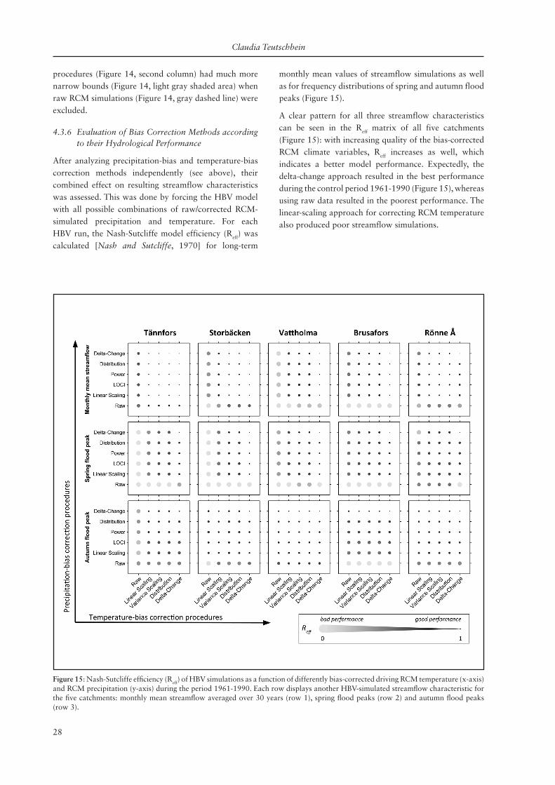
Claudia Teutschbein

28

procedures (Figure 14, second column) had much more narrow bounds (Figure 14, light gray shaded area) when raw RCM simulations (Figure 14, gray dashed line) were excluded.

4.3.6 Evaluation of Bias Correction Methods according to their Hydrological Performance

After analyzing precipitation-bias and temperature-bias correction methods independently (see above), their combined effect on resulting streamflow characteristics was assessed. This was done by forcing the HBV model with all possible combinations of raw/corrected RCM-simulated precipitation and temperature. For each HBV run, the Nash-Sutcliffe model efficiency (Reff) was calculated [Nash and Sutcliffe, 1970] for long-term

monthly mean values of streamflow simulations as well as for frequency distributions of spring and autumn flood peaks (Figure 15).

A clear pattern for all three streamflow characteristics can be seen in the Reff matrix of all five catchments (Figure 15): with increasing quality of the bias-corrected RCM climate variables, Reff increases as well, which indicates a better model performance. Expectedly, the delta-change approach resulted in the best performance during the control period 1961-1990 (Figure 15), whereas using raw data resulted in the poorest performance. The linear-scaling approach for correcting RCM temperature also produced poor streamflow simulations.

Figure 15: Nash-Sutcliffe efficiency (Reff) of HBV simulations as a function of differently bias-corrected driving RCM temperature (x-axis) and RCM precipitation (y-axis) during the period 1961-1990. Each row displays another HBV-simulated streamflow characteristic for the five catchments: monthly mean streamflow averaged over 30 years (row 1), spring flood peaks (row 2) and autumn flood peaks (row 3).


29

Figure 16: Performance of different precipitation-bias corrections (white shaded area) and their ensemble median (dark gray curve) for designed calibration (dry years, blue) and validation period (wet years, orange) compared to observations (black circles) on an annual basis in the Brusafors river basin (#4) in southern Sweden. After arranging the years in order of ascending precipitation and splitting them into calibration (drier years) and validation (wetter years) period, the precipitation residuals were computed as the relative difference between RCM-simulated and observed (representing 100%) annual precipitation values.

Figure 17: Performance of different temperature-bias corrections (white shaded area) and their ensemble median (dark gray curve) for designed calibration (cold years, blue) and validation period (warm years, orange) compared to observations (black circles) in the Storbäcken river basin (#2) in northern Sweden. After arranging the years in order of ascending temperature and splitting them into calibration (colder years) and validation (warmer years) period, the temperature residuals were computed as the difference between RCM-simulated and observed annual values. Please note the different scale of the upper left subplot (raw RCM simulations).

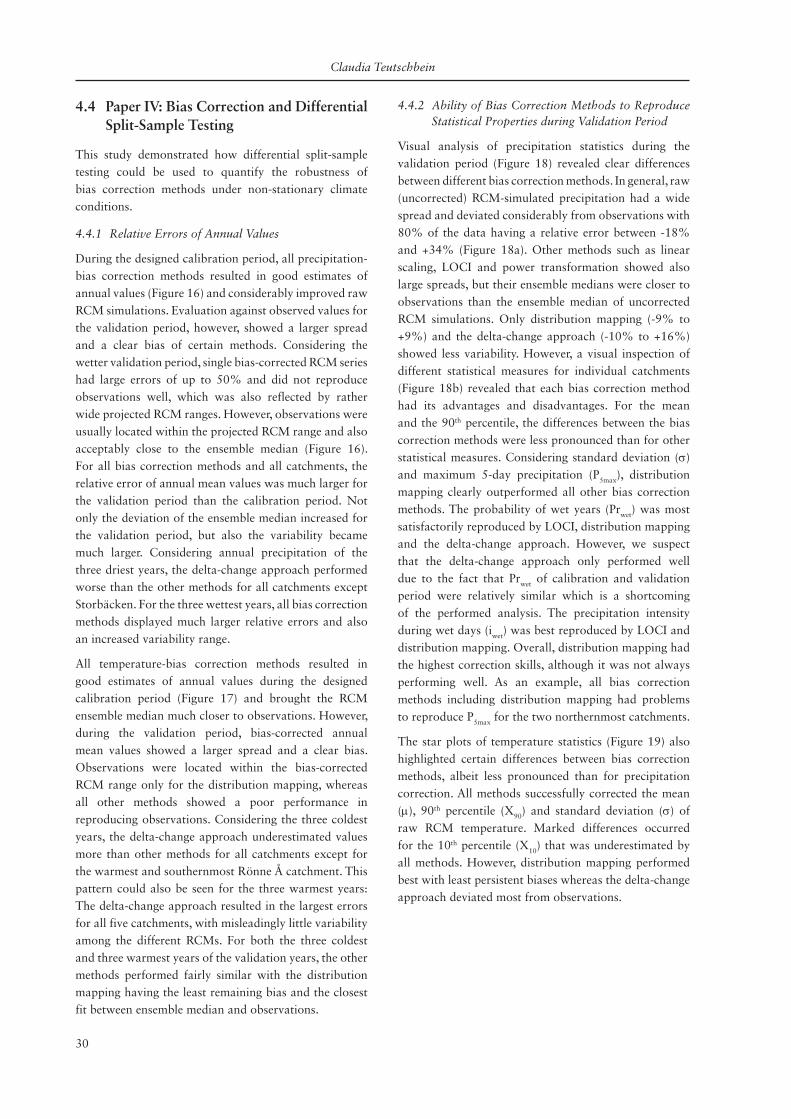
Claudia Teutschbein

30

4.4 Paper IV: Bias Correction and Differential Split-Sample Testing

This study demonstrated how differential split-sample testing could be used to quantify the robustness of bias correction methods under non-stationary climate conditions.

4.4.1 Relative Errors of Annual Values

During the designed calibration period, all precipitation-bias correction methods resulted in good estimates of annual values (Figure 16) and considerably improved raw RCM simulations. Evaluation against observed values for the validation period, however, showed a larger spread and a clear bias of certain methods. Considering the wetter validation period, single bias-corrected RCM series had large errors of up to 50% and did not reproduce observations well, which was also reflected by rather wide projected RCM ranges. However, observations were usually located within the projected RCM range and also acceptably close to the ensemble median (Figure 16). For all bias correction methods and all catchments, the relative error of annual mean values was much larger for the validation period than the calibration period. Not only the deviation of the ensemble median increased for the validation period, but also the variability became much larger. Considering annual precipitation of the three driest years, the delta-change approach performed worse than the other methods for all catchments except Storbäcken. For the three wettest years, all bias correction methods displayed much larger relative errors and also an increased variability range.

All temperature-bias correction methods resulted in good estimates of annual values during the designed calibration period (Figure 17) and brought the RCM ensemble median much closer to observations. However, during the validation period, bias-corrected annual mean values showed a larger spread and a clear bias. Observations were located within the bias-corrected RCM range only for the distribution mapping, whereas all other methods showed a poor performance in reproducing observations. Considering the three coldest years, the delta-change approach underestimated values more than other methods for all catchments except for the warmest and southernmost Rönne Å catchment. This pattern could also be seen for the three warmest years: The delta-change approach resulted in the largest errors for all five catchments, with misleadingly little variability among the different RCMs. For both the three coldest and three warmest years of the validation years, the other methods performed fairly similar with the distribution mapping having the least remaining bias and the closest fit between ensemble median and observations.

4.4.2 Ability of Bias Correction Methods to Reproduce Statistical Properties during Validation Period

Visual analysis of precipitation statistics during the validation period (Figure 18) revealed clear differences between different bias correction methods. In general, raw (uncorrected) RCM-simulated precipitation had a wide spread and deviated considerably from observations with 80% of the data having a relative error between -18% and +34% (Figure 18a). Other methods such as linear scaling, LOCI and power transformation showed also large spreads, but their ensemble medians were closer to observations than the ensemble median of uncorrected RCM simulations. Only distribution mapping (-9% to +9%) and the delta-change approach (-10% to +16%) showed less variability. However, a visual inspection of different statistical measures for individual catchments (Figure 18b) revealed that each bias correction method had its advantages and disadvantages. For the mean and the 90th percentile, the differences between the bias correction methods were less pronounced than for other statistical measures. Considering standard deviation (s) and maximum 5-day precipitation (P5max), distribution mapping clearly outperformed all other bias correction methods. The probability of wet years (Prwet) was most satisfactorily reproduced by LOCI, distribution mapping and the delta-change approach. However, we suspect that the delta-change approach only performed well due to the fact that Prwet of calibration and validation period were relatively similar which is a shortcoming of the performed analysis. The precipitation intensity during wet days (iwet) was best reproduced by LOCI and distribution mapping. Overall, distribution mapping had the highest correction skills, although it was not always performing well. As an example, all bias correction methods including distribution mapping had problems to reproduce P5max for the two northernmost catchments.

The star plots of temperature statistics (Figure 19) also highlighted certain differences between bias correction methods, albeit less pronounced than for precipitation correction. All methods successfully corrected the mean (m), 90th percentile (X90) and standard deviation (s) of raw RCM temperature. Marked differences occurred for the 10th percentile (X10) that was underestimated by all methods. However, distribution mapping performed best with least persistent biases whereas the delta-change approach deviated most from observations.


31

Figure 18: Statistical performance comparison of different bias correction methods (different axes of the star plots) for precipitation of the validation period (wetter years) as simulated by different RCMs (orange lines). The bias correction methods were parameterized based on the calibration period (drier years). The results were standardized based on observations (black circles) for the validation period. Subplot (a) summarizes all graphics of subplot (b) and gives an explanation on how to interpret the graphics. Subplot (b) breaks down subplot (a) into several catchment locations and statistical measures.

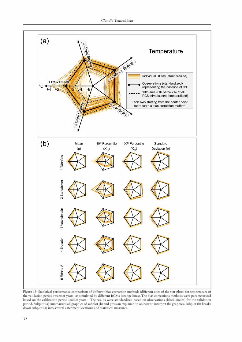
Claudia Teutschbein

32

Figure 19: Statistical performance comparison of different bias correction methods (different axes of the star plots) for temperature of the validation period (warmer years) as simulated by different RCMs (orange lines). The bias corrections methods were parameterized based on the calibration period (colder years). The results were standardized based on observations (black circles) for the validation period. Subplot (a) summarizes all graphics of subplot (b) and gives an explanation on how to interpret the graphics. Subplot (b) breaks down subplot (a) into several catchment locations and statistical measures.


33

5 dIscussIon

5.1 Climate Change and Hydrology

The coupling of climate model output and hydrological models is still challenging. Climate models have been frequently used in recent years to provide hydrologists with meteorological input data. Coherent scientific standards for adequate post-processing of climate model simulations have, however, not yet been established. This thesis discusses challenges related to using climate model output for regional hydrological impact studies as well as possible strategies to address them. Ultimately, this thesis will hopefully contribute towards the development of scientifically-approved standard procedures.

5.2 Downscaling Climate Models from Global to Catchment Scale

5.2.1 Choice of Downscaling Method

Choosing an appropriate downscaling method at the beginning of a new study still poses a major challenge for most hydrological impact modelers. Unfortunately, literature does not provide a clear answer on whether statistical (SD) or dynamical downscaling (DD) is to be preferred and under which conditions. Depending on the analyzed climate variable, statistical measure, season, region, temporal or spatial scale and many more, SD can outperform DD or vice versa [Murphy, 1999; Wilby et al., 2000; Wood et al., 2004; Díez et al., 2005; Spak et al., 2007; Prudhomme and Davies, 2009a]. A couple of influencing factors have to be considered. For example, a lot of time can be saved if RCM runs are already available from archives (e.g., PRUDENCE or ENSEMBLES) for the region of interest. Furthermore, the available computing power and time to conduct a study can be decisive factors for choosing between the computationally cheaper SD and the computationally more demanding DD. Other factors such as scales (temporal and spatial), available data (e.g., for calibration) or number of climate variables to be downscaled need to be considered as well.

5.2.2 Statistical Downscaling

The results of the downscaling study with multiple statistical downscaling approaches (Paper I) showed that the choice of downscaled precipitation time series had a major impact on the streamflow simulations. This was directly related to the ability of the downscaling approaches to reproduce observed precipitation. There

were considerable differences between different SD approaches, with AM having the largest spread in precipitation and SDSM having the smallest. SDSM turned out as the best downscaling method to reproduce observed precipitation series for winter and spring. Yet, SDSM was not necessarily the best approach for autumn precipitation, which points out the importance of a multi-model approach in climate impact studies.

5.2.3 Dynamical Downscaling

Although RCMs simulate surface runoff in addition to climate variables, they were unable to realistically simulate surface runoff, as demonstrated in Paper II using the example of five Swedish catchments. This is partly due to the fact that RCM runoff schemes are not necessarily designed to simulate discharge accurately but respond only to general tendencies in the water balance [Van den Hurk et al., 2005]. Thus, the hydrological output variables from current state-of-the-art RCMs cannot be used directly for hydrological impact studies without adequate post-processing.

The coupling of RCM climate output and hydrological modeling is also subject to considerable variability which cannot be appropriately represented by a single RCM. This was clearly demonstrated by the large inter-model variability of RCMs when applying a multi-RCM approach for streamflow simulations in meso-scale catchments in Sweden (Paper II). Thus, crucial information can potentially be lost by using only a single RCM (S-RCM). It is therefore remarkable that many current publications are still based on the S-RCM approach to make a projection of future climate change impacts. There are reasons for S-RCM approaches, such as limited computing power in older studies, very large catchment sizes or developing and testing of new methods, but in general it is difficult to justify the S-RCM approach. If the catchment extends over a couple of climate model grid cells, further scaling is, in most cases, not applied (e.g., Jha et al. [2004], Lee et al. [2004], Payne et al. [2004], Wood et al. [2004], Kleinn et al. [2005] or Kilsby et al. [2007]). This can be justified by the fact that deviations of RCM-simulated climate data from observations are mostly averaged out at larger spatial scales, leading to similar performances of the hydrological model [Dankers et al., 2007]. However, even in relatively large catchments, outcomes can vary from RCM to RCM (e.g., Graham et al. [2007b]). Using the S-RCM approach for developing or testing purposes

Claudia Teutschbein

34

(e.g., Wood et al. [2004], Kay et al. [2006a, 2006b], Bell et al. [2007a, 2007b], Leander and Buishand [2007] or Beldring et al. [2008]) can be useful to reduce the labor and computing power demand of ensemble simulations. For these purposes, such a simple modeling chain might be a suitable start. Nevertheless, these methods should also be tested on a modeling chain with additional RCMs. Kay et al. [2006b, p.171], for instance, remind the reader that their “results should not be treated as

predictions of what will happen […] in the future, as they

rely on a single run of a single RCM/GCM combination

for a single emission scenario”. They concluded that the mean of several RCM-ensemble members would give a better representation of current and future conditions. Thus, ensemble runs would reduce the risk of systematic errors and would allow a more accurate assessment of the variability in the projections. According to Weigel et al. [ 2009], multi-model ensembles widen the ensemble spread and entail an improved forecast reliability of the ensemble median. The S-RCM approach should thus be limited to pilot studies and should be strictly avoided in any climate change impact study.

Taking into account the uncertainties linked to any member of the modeling chain and neglecting the few aforementioned justified exceptions, only ensemble-based RCM (E-RCM) studies (e.g., Horton et al. [2006], Bürger et al. [2007], de Wit et al. [2007] or Graham et al. [2007a]) should be regarded as good scientific practice. Both previous studies [Horton et al., 2006; de Wit et al., 2007] and the case study presented in Paper II further demonstrated that the streamflow ensemble median fitted observations better than individual models. This indicates that E-RCM approaches lead to more robust and reliable projections than S-RCM approaches. It is, however, worthwhile noting that an ensemble projection is influenced by (1) the number of models, (2) the inter-model independency and (3) the occurrence of systematic biases [Weigel et al., 2009].

In an ensemble projection, individual RCMs are usually given equal weight. One could, however, also argue that models that perform better for current conditions should also be given more weight in the ensemble projection. In other words, the performance of an individual model (or model chain) for current conditions could serve as weighing factor (likelihood measure) when computing the ensemble statistics. Weighting of RCMs is a relatively new topic within the field of regional climate modeling. However, it has been shown that weighted ensembles do not necessarily perform better than unweighted ensembles due to a lack of sufficient inter-model independency [Fowler and Ekström, 2009]. Moreover,

there is usually no scientific basis for absolute rejection of a certain hypothesis [Spear and Hornberger, 1980], i.e., in this context the exclusion of a certain RCM. In fact, it is not clear whether the best-performing RCMs actually reproduce current conditions for the right reasons (i.e., better process representation) or just by chance.

Results from Paper II and previous studies [Varis et al., 2004; Christensen et al., 2008] also proved that RCM simulations are often biased. Thus, bias correction is recommended when using RCM output for hydrological modeling. However, one should be aware that additional bias correction in the modeling chain might add uncertainties in climate change impacts studies.

5.3 Bias Correction of Downscaled Climate Model Data

Uncorrected RCM simulations were identified in Paper III as potential source of systematic errors and large uncertainties when used as input to hydrological impact studies. The detected temperature and precipitation biases conform to findings in previous studies [Rummukainen et al., 2001; Kjellström et al., 2005, 2011; Graham et al., 2007b; Jacob et al., 2007; Teutschbein and Seibert, 2010]. A biased mean sea level pressure (MSLP) in the GCM data driving the RCMs can partially explain these biases [Jacob et al., 2007]. However, similarly distinct biases also occur even when the RCMs are forced with ‘almost perfect’ boundary conditions (i.e., with re-analysis products) instead of GCMs [Kotlarski et al., 2005; Jaeger et al., 2008; Teutschbein and Seibert, 2010]. This indicates that the dominant portion of the biases is likely introduced by the RCMs themselves. Therefore, there is a need for bias correction procedures to ensure that RCM biases do not hamper subsequent impact simulations. This doctoral thesis is neither an attempt to answer the “main question […], whether and when

the application of bias correction methods […] is

justified or not” [Ehret et al., 2012, p.3392] nor to discuss several problematic aspects related to bias correction [Ehret et al., 2012]. Rather, it is an attempt to fill the obvious gap formed by the great demand for hydrological projections and the current lack of viable alternatives to this way of post-processing RCM data. Although theoretical alternatives such as improved climate models with more detailed process simulations and increased spatial resolutions have been suggested [Teutschbein and Seibert, 2010, 2012a; Teutschbein et

al., 2011; Ehret et al., 2012; Muerth et al., 2012], it seems unlikely that these will be operational in the near future.


35

All applied bias correction approaches improved the raw RCM data to some extent. Nonetheless, the quality of adjusted RCM temperature and precipitation was strongly dependent on the choice of the correction algorithm, both for current and future climate conditions. The delta-change approach uses observations as a basis and, thus, is a stable and robust method that produces future time series with dynamics similar to current conditions. But its design also directly implies that the delta-change approach cannot account for potential future changes in climate dynamics, e.g., the number of dry vs. wet days does not change [Graham et al., 2007a]. Another shortcoming is the fact that major events (e.g., heavy precipitation or hot days) will change by the same amount as all other events (e.g., drizzle or cold days). To overcome these issues, more sophisticated versions of the delta-change approach have recently been developed [Chiew et al., 2009; Olsson et al., 2009; Anandhi et al., 2011; Bosshard et al., 2011]. These methods perform better based on an adjusted temporal scale, temporal resolution, mathematical formulation or number of change factors [Anandhi et al., 2011], but they are, as a matter of course, more difficult to apply for an impact modeler who seeks to quickly improve impact simulations. The linear-scaling approach adjusts monthly mean values and yields corrected data with a variability that is more consistent with the original RCM data [Graham et al., 2007a]. Similar to the delta-change approach, the downside is that all events are adjusted with the same correction factor. Furthermore, it is impossible to correct frequencies with the linear-scaling approach. Local Intensity Scaling (LOCI) is an improvement of the linear-scaling approach, because it combines the linear-scaling advantages with a correction of wet-day frequencies (precipitation threshold). Both power transformation and variance scaling adjust the variance and the mean of raw RCM data. These methods also perform much better than the previous approaches in terms of correcting several statistical characteristics and in terms of the variability range. Although the power transformation corrects percentiles and the coefficient of variation to some extent, it still does not give corrected RCM data with accurate probability of dry days and precipitation intensity. As a result, this nonlinear transformation may do less well for RCM simulations with a large bias in wet-day frequency [Leander and Buishand, 2007]. Distribution mapping was found to be the most reliable correction method in this study. It corrects most of the statistical characteristics and has the narrowest variability ranges, combined with the best fit of the ensemble median. The main drawback of this method is that it is - just like all other methods in this study - based on the stationarity assumption that the

same correction algorithm applies to both current and future climate conditions. A possible approach to solving this issue could be the consideration of a time-dependent bias [Buser et al., 2009], which would require an analysis of model bias behavior over a longer time period. However, such a method has not yet been fully developed and entails further assumptions for distinguishing bias changes from climate change [Buser et al., 2009]. Furthermore it should be noted that none of the applied correction methods takes the physical causes of the precipitation and temperature biases into account (e.g., temporal errors in major circulation systems or errors in the parameterization of cloud and precipitation processes). Since these biases are partly related to biases in driving GCM data, a more natural alternative could be to adjust existing biases before coupling GCMs and RCMs.

The assessment of different bias correction procedures in Paper III quantified their ability to improve raw RCM data for current climate conditions. In practice, however, it is often more interesting to know how bias correction procedures perform under changed conditions. While it is impossible to measure performances under future conditions, Paper IV illustrated the use of differential split-sample testing (DSST) to evaluate the transferability of bias correction approaches to different climate conditions. The transferability of a bias correction procedure can be described as its skill to reproduce climate characteristics of a period that differs considerably from the period used for calibrating the procedure. Low performance measures are thus indicators for poor transferability or inadequacy of the procedure. Although testing of the transferability of bias correction methods by calibrating them with the 15 coldest/driest years and validating them with the 15 warmest/wettest years might seem extreme, we argue that it allows a more reliable assessment of extreme years. This is also important for analyzing climate impacts on critical hydrological phenomena such as droughts or flood. It is worth noting that the way of splitting a 30-year period as done in Paper IV might still produce too little differences between calibration and validation period, which could potentially lead to an underestimated future climate change. However, even longer time series of consistent climate records to overcome this limitation are relatively rare.

The delta-change and the linear-scaling approach are the two most common transfer methods and have been widely used [Gellens and Roulin, 1998; Lettenmaier et al., 1999; Middelkoop et al., 2001; Shabalova et al., 2003; Fowler and Kilsby, 2007; Fowler et al., 2007; Graham et al., 2007a, 2007b; Walsh and Kilsby, 2007; Moore et al., 2008]. Both are

Claudia Teutschbein

36

appealing for impact modelers, because they are simple and rather straightforward to implement. Yet, these two methods performed particularly poor in the DSST conducted in Paper IV. When validated, both approaches resulted in larger, systematic deviations with too narrow E-RCM variability bounds that did not even include observational data. In other words, the delta-change and the linear scaling approaches were not only the least reliable for future projections but provided also wrong and overconfident uncertainty ranges. Although these findings remain to be confirmed for other catchments and geographic regions, the findings in Paper IV strongly suggest that the delta-change and the linear-scaling approach are inadequate or, at least, very questionable choices for bias-correcting RCM scenarios of future conditions.

In conclusion, the selection of one or several bias correction algorithms has a strong influence on the results of hydrological change assessments. While choosing an adequate algorithm for application under current conditions is a rather simple task, the selection of an appropriate bias correction procedure for future conditions is much more challenging. In this case, the transferability of different methods from current to changed conditions plays a fundamental role. The differential split-sample test proved to be a suitable tool for evaluating this transferability. It attested high-skill methods (e.g., distribution mapping) a much better transferability than simple methods (e.g., delta-change approach).

5.4 Hydrological Modeling of Climate-Change Impacts

Both downscaling and bias correction strongly affected hydrological simulations. Generally, correcting biases of RCM output for hydrological modeling under current conditions substantially improved streamflow simulations (Paper III). Hydrological simulations driven with the higher-skill (e.g., distribution mapping) bias-corrected RCM data performed generally better than corresponding simulations driven with lower-skill (e.g., linear scaling) bias-corrected RCM data. Of all tested methods, distribution mapping performed best in terms of transferability and robustness for projections of hydrological extremes. Furthermore, variability ranges produced by better-performing correction algorithms were also less wide than those of less well-performing algorithms. However, much of the variability in streamflow simulations occurred independently of the bias correction procedures and originated from inter-RCM variability and uncertain hydrological model parameters. Due to the long and complex modeling chain,

it was therefore challenging to reduce the remaining uncertainty in the hydrological projections.

Major future changes in annual temperature and precipitation cycles were projected for all studied catchments independently from the chosen downscaling method (SD versus DD). A considerable increase in temperature combined with changes in the precipitation pattern is expected to change current flow regimes in Sweden from snowmelt-driven (with peak flows in April) to rather damped regimes with considerable streamflow volumes discharging during winter. Spring flood events (freshets) are expected to occur earlier and to decrease considerably in intensity and volume. Autumn flood peaks, on the other hand, are projected to increase only slightly. These findings also agree with earlier studies over Scandinavia [Xu, 2000; Bergström et al., 2001; Beldring et al., 2008; Moore et al., 2008]. Flow pattern changes during the cold season can possibly be explained by a projected substantial temperature increase. Higher temperatures will likely limit the accumulation of large amounts of snow while simultaniously increasing the number of rainy days. Snowmelt will be initialized earlier, causing the spring flood peak to occur one to two months earlier and to be less pronounced. Changes in spring flood timing and magnitude might lead to lower summer base flow.

Although the overall trend of projected future changes was similar for all catchments, the amount of projected change depended largely on the geographic catchment location. Especially subarctic catchments, such as the two northernmost study sites, were highly sensitive to changing climate conditions. Catchments in this region will likely display the most pronounced decrease in spring flood peak and the largest increase in winter streamflow. Though less pronounced, projected changes for southern catchments are also substantial.

5.5 Uncertainties in the Modeling Chain

The range of variability in streamflow simulations was largely influenced by the design of the modeling chain. Considering statistical downscaling (Paper I), the choice of the precipitation downscaling method had a major impact: the performance of simulated seasonal streamflow was directly related to the ability of the respective downscaling method to reproduce seasonal precipitation patterns. With respect to annual precipitation patterns, the analog sorting method (AM) displayed the largest and the statistical-downscaling model (SDSM) the smallest variation, which was directly reflected in the associated hydrological simulations. Overall, SDSM was the most suitable method for downscaling precipitation. However,


37

using more than one method increases the probability of capturing future variability. The variability of projected streamflow caused by different choices of GHG emission scenarios and GCMs appeared small compared to the variability related to different downscaling methods. It should, however, be noted that even relatively small perturbations at the beginning of the modeling chain are not necessarily negligible: Nonlinear interactions between errors that are propagated through the modeling chain can amplify themselves and ultimately result in highly unlikely streamflow projections. It can be expected that the probability for such outliers to pass unrecognized is relatively high if only a single modeling chain is considered. Ensemble approaches should therefore be regarded as good scientific practice. The same applies for

dynamical downscaling (Paper III). Despite the relatively large variability in resulting streamflow simulations (primarily caused by the inter-RCM variability and different hydrological parameter sets), it was still possible to obtain meaningful hydrological projections by applying an ensemble approach (Paper III): The ensemble median of hydrological simulations driven with corrected RCM data matched well with hydrological simulations forced by observed climate variables. This fact enhanced the confidence in future hydrological ensemble projections. Thus, it is generally possible to project overall trends of future streamflow with help of a robust ensemble. As a consequence, an ensemble approach should be part of any scientific standard procedure for conducting impact studies.

6 conclusIons

This doctoral thesis evaluated strategies for incorporating climate model output into hydrological studies to produce meaningful projections that are also reliable under changing climate conditions. A strong focus was on the assessment of the combined effects of various sources of variability on projected streamflow seasonality and peaks. The main conclusions can be summarized as follows:

• Sources of Variability: In climate change impact studies, different sources of variability can affect the results. Especially the choice of (1) future GHG emission scenarios, (2) climate models and their parameterization, (3) downscaling/post-processing techniques and (4) hydrological models and their parameterization are considered to have the largest impact.

• Value of Ensemble Projections: Depending on the choices made in the modeling chain, resulting streamflow simulations are highly variable. For that reason, full ensembles of GHG emission scenarios, climate models, downscaling methods, post-processing techniques and hydrological models should be considered standard practice to obtain meaningful hydrological projections under changing climate conditions.

• Need for Bias Correction: Substantial biases in RCM simulations need to be corrected to ensure that subsequent impact simulations are not hampered.

• Benefit of Bias Correction: Bias correction procedures substantially improve RCM-simulated climate variables and subsequent streamflow simulations under current conditions.

• Evaluating Bias Correction under Non-Stationary Conditions: Bias correction procedures are assumed to not change over time, i.e., to be transferable to changed climate conditions. The differential split-sample test is a suitable tool for evaluating this transferability of bias correction algorithms.

• Performance of different Bias Correction Methods under Non-Stationary Conditions: The differential split-sample test attests high-skill methods a much better transferability than simple methods. Of all tested methods, distribution mapping performed best in terms of transferability and robustness for projections of hydrological extremes. The delta-change and the linear-scaling approach are not recommended for bias-correcting RCM scenarios of future conditions.

• Hydrological Projections: Current flow regimes in Sweden with a snowmelt-driven spring flood in April will likely change to rather damped flow regimes that are characterized by earlier and decreased spring floods as well as large winter streamflows.

Claudia Teutschbein

38

This thesis highlighted several challenges when using state-of-the-art climate model simulations for hydrological impact studies. Amongst others, one general challenge is the imperfect representation of atmospheric processes in climate models [Maraun, 2012]. For instance, climate models fail to resolve meso-scale and short-lived weather systems such as arctic fronts and polar lows [Kolstad

and Bracegirdle, 2008; Zahn and von Storch, 2010; Condron and Renfrew, 2012]. However, latest research results show that such systems can be of great importance for larger-scale circulations and climate projections [Condron and Renfrew, 2012]. Thus, a long-term goal lies in the enhancement of climate models to include more detailed relevant processes and to run at higher spatial resolutions [Teutschbein and Seibert, 2010, 2012a; Teutschbein et al., 2011; Ehret et al., 2012; Muerth et al., 2012]. In the meantime, however, there is a clear demand for developing more robust tools and assessment strategies that are capable of dealing with imperfect climate model output and producing reliable data for hydrological impact modelers.

My own plans for future research include the following two already ongoing projects. The first project is a continuation of the evaluation of bias correction methods. As mentioned earlier, the differential split-sample test does not allow performing hydrological simulations, because the split bias-corrected temperature and precipitation periods consist of different years and do not correspond to each other. To overcome this issue,

7 Future research

it is planned to shift this so-called univariate differential split-sample test to a bivariate test which would allow using the bias-corrected precipitation and temperature series as combined input for streamflow simulations. The bivariate differential-split sample could hypothetically also be extended to a multivariate test depending on the number of climate variables required for the hydrological simulations. With such a bi- or multivariate differential split-sample test it would be possible to demonstrate whether bias-correction methods are a feasible technique to deal with biases in RCM output for hydrological impact studies under non-stationary conditions or not.

The second project strikes out in a new direction: Potential evaporation is an important input variable when simulating streamflow and especially low-flow events. For climate change impact studies, however, it is often not clear how to best derive this variable from RCM simulations, i.e., directly (from RCMs) or through empirical or physically-based relationships to other climate variables. Preliminary results indicate that direct potential evaporation provided by climate model simulations is strongly biased and not suitable for direct use in hydrological models. Further investigations are thus needed to evaluate the performance and reliability of several potential evapotranspiration estimates ranging from simple empirical to data-intensive and rather sophisticated process-oriented methods in a climate change context.

8 reFerences

Anandhi, A., A. Frei, D. C. Pierson, E. M. Schneiderman, M. S. Zion, D. Lounsbury, and A. H. Matonse (2011), Examination of change factor methodologies for climate change impact assessment, Water Resour Res, 47(3), W03501, doi:10.1029/2010WR009104.

Bardossy, A., and E. J. Plate (1992), Space-time model for daily rainfall using atmospheric circulation patterns, Water Resour Res, 28(5), 1247–1259, doi:10.1029/91WR02589.

Bardossy, A., L. Duckstein, and I. Bogardi (1995), Fuzzy rule-based classification of atmospheric circulation patterns, Int J Climatol, 15(10), 1087–1097, doi:10.1002/joc.3370151003.

Bardossy, A., J. Stehlík, and H.-J. Caspary (2001), Generating of areal precipitation series in the upper Neckar catchment, Phys Chem Earth PT B, 26(9), 683–687, doi:10.1016/S1464-1909(01)00069-7.

Bardossy, A., I. Bogardi, and I. Matyasovszky (2005), Fuzzy rule-based downscaling of precipitation, Theor Appl Climatol, 82(1), 119–129, doi:10.1007/s00704-004-0121-0.

Beldring, S., T. Engen-Skaugen, E. J. Førland, and L. A. Roald (2008), Climate change impacts on hydrological processes in Norway based on two methods for transferring regional climate model results to meteorological station sites, Tellus A, 60(3), 439–450, doi:10.1111/j.1600-0870.2008.00306.x.

Bell, V. A., A. L. Kay, R. G. Jones, and R. J. Moore (2007a), Development of a high resolution grid-based river flow model for use with regional climate model output, Hydrol Earth Syst Sci, 11(1), 532–549, doi:10.5194/hess-11-532-2007.

Bell, V. A., A. L. Kay, R. G. Jones, and R. J. Moore (2007b), Use of a grid-based hydrological model and regional


39

climate model outputs to assess changing flood risk, Int J Climatol, 27(12), 1657–1671, doi:10.1002/joc.1539.

Bennett, J. C., F. L. N. Ling, B. Graham, M. R. Grose, S. P. Corney, C. J. White, G. K. Holz, D. A. Post, S. M. Gaynor, and N. L. Bindoff (2010), Climate Futures for Tasmania: Water and Catchments., Technical Report, Antarctic Climate & Ecosystems Cooperative Research Centre, Hobart, Tasmania.

Bergström, S. (1976), Development and application of a conceptual runoff model for Scandinavian catchments, Report RHO 7, SMHI, Norrköping, Sweden.

Bergström, S. (1992), The HBV model - its structure and applications, Hydrologi Report RH 4, SMHI, Norrköping, Sweden.

Bergström, S., B. Carlsson, M. Gardelin, G. Lindström, A. Pettersson, and M. Rummukainen (2001), Climate change impacts on runoff in Sweden – assessments by global climate models, dynamical downscaling and hydrological modelling, Clim Res, 16, 101–112, doi:10.3354/cr016101.

Beven, K. J. (2002), Rainfall - Runoff Modelling: The Primer, 1st ed., John Wiley & Sons, Chinchester, England.

Block, P. J., F. A. Souza Filho, L. Sun, and H. H. Kwon (2009), A Streamflow Forecasting Framework using Multiple Climate and Hydrological Models1, J Am Water Resour As, 45(4), 828–843, doi:10.1111 ⁄ j.1752-1688.2009.00327.x.

Boe, J., L. Terray, F. Habets, and E. Martin (2007), Statistical and dynamical downscaling of the Seine basin climate for hydro-meteorological studies, Int J Climatol, 27(12), 1643–1655, doi:10.1002/joc.1602.

Bosshard, T., S. Kotlarski, T. Ewen, and C. Schär (2011), Spectral representation of the annual cycle in the climate change signal, Hydrol Earth Syst Sci, 15, 2777–2788, doi:10.5194/hess-15-2777-2011.

Bowden, J. H., T. L. Otte, C. G. Nolte, and M. J. Otte (2011), Examining Interior Grid Nudging Techniques Using Two-Way Nesting in the WRF Model for Regional Climate Modeling, J Climate, 25(8), 2805–2823, doi:10.1175/JCLI-D-11-00167.1.

Buser, C. M., H. R. Künsch, D. Lüthi, M. Wild, and C. Schär (2009), Bayesian multi-model projection of climate: bias assumptions and interannual variability, Clim Dynam, 33(6), 849–868, doi:10.1007/s00382-009-0588-6.

Bürger, C., O. Kolditz, H. Fowler, and S. Blenkinsop (2007), Future climate scenarios and rainfall–runoff modelling in the Upper Gallego catchment (Spain), Environ Pollut, 148(3), 842–854, doi:10.1016/j.envpol.2007.02.002.

Cameron, D. (2006), An application of the UKCIP02 climate change scenarios to flood estimation by continuous simulation for a gauged catchment in the northeast of Scotland, UK (with uncertainty), J Hydrol, 328(1–2), 212–226, doi:10.1016/j.jhydrol.2005.12.024.

Chan, S., E. Kendon, H. Fowler, S. Blenkinsop, C. T. Ferro, and D. Stephenson (2012), Does increasing the spatial resolution of a regional climate model improve the simulated daily precipitation?, Clim Dyn, 1–21, doi:10.1007/s00382-012-1568-9.

Chen, J., F. P. Brissette, A. Poulin, and R. Leconte (2011a), Overall uncertainty study of the hydrological impacts of climate change for a Canadian watershed, Water Resour Res, 47(12), W12509, doi:10.1029/2011WR010602.

Chen, J., F. P. Brissette, and R. Leconte (2011b), Uncertainty of downscaling method in quantifying the impact of climate change on hydrology, J Hydrol, 401(3-4), 190–202,

doi:10.1016/j.jhydrol.2011.02.020.

Chiew, F. H. S., J. Teng, J. Vaze, D. A. Post, J. M. Perraud, D. G. C. Kirono, and N. R. Viney (2009), Estimating climate change impact on runoff across southeast Australia: Method, results, and implications of the modeling method, Water Resour Res, 45(10), W10414, doi:10.1029/2008WR007338.

Christensen, J., T. Carter, M. Rummukainen, and G. Amanatidis (2007), Evaluating the performance and utility of regional climate models: the PRUDENCE project, Climatic Change, 81, 1–6, doi:10.1007/s10584-006-9211-6.

Christensen, J. H., F. Boberg, O. B. Christensen, and P. Lucas-Picher (2008), On the need for bias correction of regional climate change projections of temperature and precipitation, Geophys Res Lett, 35(20), L20709, doi:10.1029/2008GL035694.

Condron, A., and I. A. Renfrew (2012), The impact of polar mesoscale storms on northeast Atlantic Ocean circulation, Nat Geosci, doi:10.1038/ngeo1661.

Coron, L., V. Andréassian, C. Perrin, J. Lerat, J. Vaze, M. Bourqui, and F. Hendrickx (2012), Crash testing hydrological models in contrasted climate conditions: An experiment on 216 Australian catchments, Water Resour Res, 48(5), W05552, doi:10.1029/2011WR011721.

Dankers, R., O. B. Christensen, L. Feyen, M. Kalas, and A. de Roo (2007), Evaluation of very high-resolution climate model data for simulating flood hazards in the Upper Danube Basin, J Hydrol, 347(3–4), 319–331, doi:10.1016/j.jhydrol.2007.09.055.

Déqué, M., D. P. Rowell, D. Lüthi, F. Giorgi, J. H. Christensen, B. Rockel, D. Jacob, E. Kjellström, M. De Castro, and B. van den Hurk (2007), An intercomparison of regional climate simulations for Europe: assessing uncertainties in model projections, Climatic Change, 81, 53–70, doi:10.1007/s10584-006-9228-x.

Diaz-Nieto, J., and R. L. Wilby (2005), A comparison of statistical downscaling and climate change factor methods: impacts on low flows in the River Thames, United Kingdom, Climatic Change, 69(2-3), 245–268, doi:10.1007/s10584-005-1157-6.

Dickinson, R. E., R. M. Errico, F. Giorgi, and G. T. Bates (1989), A regional climate model for the western United States, Climatic Change, 15(3), 383–422, doi:10.1007/BF00240465.

Díez, E., C. Primo, J. A. García-Moya, J. M. Gutiérrez, and B. Orfila (2005), Statistical and dynamical downscaling of precipitation over Spain from DEMETER seasonal forecasts., Tellus A, 57(3), 409–423, doi:10.1111/j.1600-0870.2005.00130.x.

Dosio, A., P. Paruolo, and R. Rojas (2012), Bias correction of the ENSEMBLES high resolution climate change projections for use by impact models: Analysis of the climate change signal, J Geophys Res, 117(D17), D17110, doi:10.1029/2012JD017968.

Ehret, U., E. Zehe, V. Wulfmeyer, K. Warrach-Sagi, and J. Liebert (2012), HESS Opinions “Should we apply bias correction to global and regional climate model data?”, Hydrol Earth Syst Sci, 16(9), 3391–3404, doi:10.5194/hess-16-3391-2012.

Evans, J. P. (2011), CORDEX – An international climate downscaling initiative, in MODSIM2011, 19th International Congress on Modelling and Simulation, edited by F. Chan, D. Marinova, and R. S. Anderssen, pp. 2705–2711, Modelling and Simulation Society of Australia and New Zealand, Perth, Australia. [online]

Claudia Teutschbein

40

Available from: http://www.mssanz.org.au/modsim2011/F5/evans.pdf (Accessed 21 December 2012)

Foley, A. M. (2010), Uncertainty in regional climate modelling: A review., Prog Phys Geog, 34(5), 647–670, doi:10.1177/0309133310375654.

Foley, J. A., M. H. Costa, C. Delire, N. Ramankutty, and P. Snyder (2003), Green surprise? How terrestrial ecosystems could affect earth’s climate, Front Ecol Environ, 1(1), 38–44, doi:10.1890/1540-9295(2003)001[0038:GSHTEC]2.0.CO;2.

Fowler, H., and C. Kilsby (2007), Using regional climate model data to simulate historical and future river flows in northwest England, Climatic Change, 80(3), 337–367, doi:10.1007/s10584-006-9117-3.

Fowler, H. J., and M. Ekström (2009), Multi-model ensemble estimates of climate change impacts on UK seasonal precipitation extremes, Int J Climatol, 29(3), 385–416, doi:10.1002/joc.1827.

Fowler, H. J., C. G. Kilsby, and J. Stunell (2007), Modelling the impacts of projected future climate change on water resources in north-west England, Hydrol Earth Syst Sci, 11(3), 1115–1126, doi:10.5194/hess-11-1115-2007.

Gellens, D., and E. Roulin (1998), Streamflow response of Belgian catchments to IPCC climate change scenarios, J Hydrol, 210(1-4), 242–258, doi:10.1016/S0022-1694(98)00192-9.

Giorgi, F. (2006), Regional climate modeling: Status and perspectives, J Phys IV, 139, 101–118, doi:10.1051/jp4:2006139008.

Goderniaux, P., S. Brouyère, H. J. Fowler, S. Blenkinsop, R. Therrien, P. Orban, and A. Dassargues (2009), Large scale surface–subsurface hydrological model to assess climate change impacts on groundwater reserves, J Hydrol, 373(1–2), 122–138, doi:10.1016/j.jhydrol.2009.04.017.

Goodess, C., C. Anagnostopoulou, A. Bárdossy, C. Frei, C. Harpham, M. Haylock, Y. Hundecha, P. Maheras, J. Ribalaygua, and J. Schmidli (2012), An intercomparison of statistical downscaling methods for Europe and European regions–assessing their performance with respect to extreme temperature and precipitation events, Climate Research Unit Research Publications: CRU RP11, University of East Anglia: UK. [online] Available from: http://www.cru.uea.ac.uk/cru/pubs/crurp/CRU_RP11.pdf (Accessed 21 December 2012)

Goodess, C. M. (2005), STARDEX: Downscaling Climate Extremes, Final Report. An EU Project funded under Framework Programme 5, European Commission DG Research. Contract number: EVK2-CT-2001-00115., Climate Research Unit, University of East Anglia: UK. [online] Available from: http://www.cru.uea.ac.uk/projects/stardex/reports/STARDEX_FINAL_REPORT.pdf (Accessed 21 December 2012)

Goodess, C. M. et al. (2005), STARDEX - Recommendations on the more robust statistical and dynamical downscaling methods for the construction of scenarios of extremes (Deliverable D16). [online] Available from: http://www.cru.uea.ac.uk/projects/stardex/deliverables/D16/D16_Summary.pdf (Accessed 21 December 2012)

Graham, L., J. Andréasson, and B. Carlsson (2007a), Assessing climate change impacts on hydrology from an ensemble of regional climate models, model scales and linking methods – a case study on the Lule River basin, Climatic Change, 81, 293–307, doi:10.1007/s10584-006-9215-2.

Graham, L., S. Hagemann, S. Jaun, and M. Beniston (2007b), On interpreting hydrological change from regional climate

models, Climatic Change, 81, 97–122, doi:10.1007/s10584-006-9217-0.

Gudmundsson, L., J. B. Bremnes, J. E. Haugen, and T. Engen-Skaugen (2012), Technical Note: Downscaling RCM precipitation to the station scale using statistical transformations - a comparison of methods, Hydrol Earth Syst Sci, 16(9), 3383–3390, doi:10.5194/hess-16-3383-2012.

Hagemann, S., C. Chen, J. O. Haerter, J. Heinke, D. Gerten, and C. Piani (2011), Impact of a Statistical Bias Correction on the Projected Hydrological Changes Obtained from Three GCMs and Two Hydrology Models, J Hydrometeorol, 12(4), 556–578, doi:10.1175/2011JHM1336.1.

Harlin, J., and C. Kung (1992), Parameter uncertainty and simulation of design floods in Sweden, J Hydrol, 137(1-4), 209–230, doi:10.1016/0022-1694(92)90057-3.

Hay, L. E., R. L. Wilby, and G. H. Leavesley (2000), A comparison of delta change and downscaled GCM scenarios for three mountainous basins in the United States, J Am Water Resour As, 36(2), 387–397, doi:10.1111/j.1752-1688.2000.tb04276.x.

Hewitson, B. C., and R. G. Crane (1996), Climate downscaling: techniques and application, Clim Res, 07(2), 85–95, doi:10.3354/cr0007085.

Horton, P., B. Schaefli, A. Mezghani, B. Hingray, and A. Musy (2006), Assessment of climate-change impacts on alpine discharge regimes with climate model uncertainty, Hydrol Process, 20(10), 2091–2109.

Van den Hurk, B., G. Lenderink, E. van Meijgaard, A. van Ulden, M. Hirschi, C. Schär, B. Rockel, S. Hagemann, P. Graham, and E. Kjellström (2005), Soil control on runoff response to climate change in regional climate model simulations, J Climate, 18(17), 3536–3551, doi:10.1175/JCLI3471.1.

Ines, A. V. M., and J. W. Hansen (2006), Bias correction of daily GCM rainfall for crop simulation studies, Agr Forest Meteorol, 138(1-4), 44–53, doi:10.1016/j.agrformet.2006.03.009.

IPCC (2001), Climate Change 2001: The Scientific Basis, Contribution of Working Group I to the Third Assessment Report of the Intergovernmental Panel on Climate Change, edited by J. T. Houghton, Y. Ding, D. J. Griggs, M. Noguer, P. J. van der Linden, X. Dai, K. Maskell, and C. Johnson, Cambridge University Press, Cambridge, UK and New York, USA.

IPCC (2007), Climate Change 2007: The Physical Science Basis, Contribution of Working Group I to the Fourth Assessment Report of the Intergovernmental Panel on Climate Change, edited by S. Solomon, D. Qin, M. Manning, Z. Chen, M. Marquis, K. B. Averyt, M. Tignor, and H. L. Miller, Cambridge University Press, Cambridge, UK, and New York, USA.

Jacob, D. et al. (2007), An inter-comparison of regional climate models for Europe: model performance in present-day climate, Climatic Change, 81, 31–52, doi:10.1007/s10584-006-9213-4.

Jaeger, E. B., I. Anders, D. Luthi, B. Rockel, C. Schar, and S. I. Seneviratne (2008), Analysis of ERA40-driven CLM simulations for Europe, Meteorol Z, 17(4), 349–367, doi:10.1127/0941-2948/2008/0301.

Jarsjö, J., S. M. Asokan, C. Prieto, A. Bring, and G. Destouni (2012), Hydrological responses to climate change conditioned by historic alterations of land-use and water-use, Hydrol Earth Syst Sci, 16(5), 1335–1347, doi:10.5194/hess-16-1335-2012.

Jha, M., Z. Pan, E. S. Takle, and R. Gu (2004), Impacts of climate


41

change on streamflow in the Upper Mississippi River Basin: A regional climate model perspective, J Geophys Res, 109, D09105, doi:10.1029/2003JD003686.

Johansson, B. (2002), Estimation of areal precipitation for hydrological modelling in Sweden. Dissertation, Earth Science Centre, Göteborg University, Report A76. Göteborg, Sweden.

Johnson, F., and A. Sharma (2011), Accounting for interannual variability: A comparison of options for water resources climate change impact assessments, Water Resour Res, 47(4), W04508, doi:10.1029/2010WR009272.

Kay, A. L., and H. N. Davies (2008), Calculating potential evaporation from climate model data: A source of uncertainty for hydrological climate change impacts, Journal of Hydrology, 358(3–4), 221–239, doi:10.1016/j.jhydrol.2008.06.005.

Kay, A. L., N. S. Reynard, and R. G. Jones (2006a), RCM rainfall for UK flood frequency estimation. I. Method and validation, J Hydrol, 318(1), 151–162, doi:10.1016/j.jhydrol.2005.06.012.

Kay, A. L., R. G. Jones, and N. S. Reynard (2006b), RCM rainfall for UK flood frequency estimation. II. Climate change results, J Hydrol, 318(1), 163–172, doi:10.1016/j.jhydrol.2005.06.013.

Kay, A. L., H. N. Davies, V. A. Bell, and R. G. Jones (2009), Comparison of uncertainty sources for climate change impacts: flood frequency in England, Climatic Change, 92(1), 41–63, doi:10.1007/s10584-008-9471-4.

Kilsby, C. G., S. S. Tellier, H. J. Fowler, and T. R. Howels (2007), Hydrological impacts of climate change on the Tejo and Guadiana Rivers, Hydrol Earth Syst Sci, 11(3), 1175–1189, doi:10.5194/hess-11-1175-2007.

Kjellström, E., L. Bärring, S. Gollvik, U. Hansson, C. Jones, P. Samuelsson, M. Rummukainen, A. Ullerstig, U. Willén, and K. Wyser (2005), A 140-year simulation of European climate with the new version of the Rossby Centre regional atmospheric climate model ( RCA3 ), Reports Meteorology and Climatology, SMHI, Norrköping, Sweden.

Kjellström, E., G. Nikulin, U. Hansson, G. Strandberg, and A. Ullerstig (2011), 21st century changes in the European climate: uncertainties derived from an ensemble of regional climate model simulations, Tellus A, 63(A), 24–40, doi:10.1111/j.1600-0870.2010.00475.x.

Kleinn, J., C. Frei, J. Gurtz, D. Lüthi, P. Vidale, and C. Schär (2005), Hydrologic simulations in the Rhine basin driven by a regional climate model, J Geophys Res, 110(D4), D04102, doi:10.1029/2004JD005143.

Klemeš, V. (1986), Operational testing of hydrological simulation models/Vérification, en conditions réelles, des modèles de simulation hydrologique, Hydrolog Sci J, 31(1), 13–24, doi:10.1080/02626668609491024.

Kolstad, E. W., and T. J. Bracegirdle (2008), Marine cold-air outbreaks in the future: an assessment of IPCC AR4 model results for the Northern Hemisphere, Clim Dyn, 30(7-8), 871–885, doi:10.1007/s00382-007-0331-0.

Kotlarski, S., A. Block, U. Bahm, D. Jacob, K. Keuler, R. Knoche, D. Rechid, and A. Walter (2005), Regional climate model simulations as input for hydrological applications: evaluation of uncertainties, Adv Geosci, 5, 119–125, doi:10.5194/adgeo-5-119-2005.

Leander, R., and T. A. Buishand (2007), Resampling of regional climate model output for the simulation of extreme river flows, J Hydrol, 332(3-4), 487–496, doi:10.1016/j.jhydrol.2006.08.006.

Leander, R., T. A. Buishand, B. J. J. M. van den Hurk, and M. J. M. de Wit (2008), Estimated changes in flood quantiles of the river Meuse from resampling of regional climate model output, J Hydrol, 351(3-4), 331–343, doi:10.1016/j.jhydrol.2007.12.020.

Lee, D. K., D. H. Cha, and H. S. Kang (2004), Regional climate simulation of the 1998 summer flood over East Asia, J Meteorol Soc Jpn, 82(6), 1735–1753, doi:10.2151/jmsj.82.1735.

Lenderink, G., A. Buishand, and W. Van Deursen (2007), Estimates of future discharges of the river Rhine using two scenario methodologies: direct versus delta approach, Hydrol Earth Syst Sci, 11(3), 1145–1159.

Lettenmaier, D. P., A. W. Wood, R. N. Palmer, E. F. Wood, and E. Z. Stakhiv (1999), Water Resources Implications of Global Warming: A U.S. Regional Perspective, Climatic Change, 43(3), 537–579, doi:10.1023/A:1005448007910.

Li, C. Z., L. Zhang, H. Wang, Y. Q. Zhang, F. L. Yu, and D. H. Yan (2012), The transferability of hydrological models under nonstationary climatic conditions, Hydrol Earth Syst Sci, 16(4), 1239–1254, doi:10.5194/hess-16-1239-2012.

Van der Linden, P., and J. F. B. Mitchell (2009), ENSEMBLES: Climate Change and its Impacts: Summary of research and results from the ENSEMBLES project, Met Office Hadley Centre, FitzRoy Road, Exeter EX1 3PB, UK. [online] Available from: http://ensembles-eu.metoffice.com/docs/Ensembles_final_report_Nov09.pdf (Accessed 21 December 2012)

Lindström, G., B. Johansson, M. Persson, M. Gardelin, and S. Bergström (1997), Development and test of the distributed HBV-96 hydrological model, J Hydrol, 201(1-4), 272–288, doi:10.1016/S0022-1694(97)00041-3.

Lobell, D., G. Bala, A. Mirin, T. Phillips, R. Maxwell, and D. Rotman (2009), Regional Differences in the Influence of Irrigation on Climate, J Climate, 22(8), 2248–2255, doi:10.1175/2008JCLI2703.1.

Lorenz, E. N. (1969), Atmospheric Predictability as Revealed by Naturally Occurring Analogues, J Atmos Sci, 26(4), 636–646, doi:10.1175/1520-0469(1969)26<636:APARBN>2.0.CO;2.

Lorenz, P., and D. Jacob (2005), Influence of regional scale information on the global circulation: A two-way nesting climate simulation, Geophys Res Lett, 32(18), L18706, doi:10.1029/2005GL023351.

Maraun, D. (2012), Nonstationarities of regional climate model biases in European seasonal mean temperature and precipitation sums, Geophys Res Lett, 39(6), L06706, doi:10.1029/2012GL051210.

Maraun, D. et al. (2010), Precipitation downscaling under climate change: Recent developments to bridge the gap between dynamical models and the end user, Rev Geophys, 48(3), RG3003, doi:10.1029/2009RG000314.

Mavromatis, T. (2012), Changes in exceptional hydrological and meteorological weekly event frequencies in Greece, Climatic Change, 110(1), 249–267, doi:10.1007/s10584-011-0095-8.

Mearns, L. O., F. Giorgi, P. Whetton, D. Pabon, M. Hulme, and M. Lal (2003), Guidelines for use of climate scenarios developed from regional climate model experiments, Data Distribution Centre of the Intergovernmental Panel on Climate Change. [online] Available from: http://www.ipcc-data.org/guidelines/dgm_no1_v1_10-2003.pdf (Accessed 21 December 2012)

Middelkoop, H., K. Daamen, D. Gellens, W. Grabs, J. C. J.

Claudia Teutschbein

42

Kwadijk, H. Lang, B. W. A. H. Parmet, B. Schädler, J. Schulla, and K. Wilke (2001), Impact of Climate Change on Hydrological Regimes and Water Resources Management in the Rhine Basin, Climatic Change, 49(1), 105–128, doi:10.1023/A:1010784727448.

Moore, K., D. Pierson, K. Pettersson, E. Schneiderman, and P. Samuelsson (2008), Effects of warmer world scenarios on hydrologic inputs to Lake Mälaren, Sweden and implications for nutrient loads, Hydrobiologia, 599(1), 191–199, doi:10.1007/s10750-007-9197-8.

Mpelasoka, F. S., and F. H. . Chiew (2009), Influence of rainfall scenario construction methods on runoff projections, J Hydrometeorol, 10(5), 1168–1183, doi:10.1175/2009JHM1045.1.

Muerth, M. J., B. Gauvin St-Denis, S. Ricard, J. A. Velázquez, J. Schmid, M. Minville, D. Caya, D. Chaumont, R. Ludwig, and R. Turcotte (2012), On the need for bias correction in regional climate scenarios to assess climate change impacts on river runoff, Hydrol Earth Syst Sci Discuss, 9(9), 10205–10243, doi:10.5194/hessd-9-10205-2012.

Murphy, J. (1999), An Evaluation of Statistical and Dynamical Techniques for Downscaling Local Climate, J Climate, 12(8), 2256–2284, doi:10.1175/1520-0442(1999)012<2256:AEOSAD>2.0.CO;2 UR.

Nash, J. E., and J. V. Sutcliffe (1970), River flow forecasting through conceptual models part I - A discussion of principles, J Hydrol, 10(3), 282–290, doi:10.1016/0022-1694(70)90255-6.

Obled, C., G. Bontron, and R. Garçon (2002), Quantitative precipitation forecasts: a statistical adaptation of model outputs through an analogues sorting approach, Atmos Res, 63(3-4), 303–324, doi:10.1016/S0169-8095(02)00038-8.

Olsson, J., K. Berggren, M. Olofsson, and M. Viklander (2009), Applying climate model precipitation scenarios for urban hydrological assessment: A case study in Kalmar City, Sweden, Atmos Res, 92(3), 364–375, doi:10.1016/j.atmosres.2009.01.015.

Payne, J. T., A. W. Wood, A. F. Hamlet, R. N. Palmer, and D. P. Lettenmaier (2004), Mitigating the effects of climate change on the water resources of the Columbia River basin, Climatic Change, 62(1), 233–256, doi:10.1023/B:CLIM.0000013694.18154.d6.

Piani, C., J. O. Haerter, and E. Coppola (2010), Statistical bias correction for daily precipitation in regional climate models over Europe, Theor Appl Climatol, 99(1), 187–192, doi:10.1007/s00704-009-0134-9.

Prudhomme, C., and H. Davies (2009a), Assessing uncertainties in climate change impact analyses on the river flow regimes in the UK. Part 1: baseline climate., Climatic Change, 93(1/2), 177–195, doi:10.1007/s10584-008-9464-3.

Prudhomme, C., and H. Davies (2009b), Assessing uncertainties in climate change impact analyses on the river flow regimes in the UK. Part 2: future climate., Climatic Change, 93(1/2), 197–222, doi:10.1007/s10584-008-9461-6.

Puma, M. J., and B. I. Cook (2010), Effects of irrigation on global climate during the 20th century, J Geophys Res, 115, D16120, doi:10.1029/2010JD014122.

Rojas, R., L. Feyen, A. Dosio, and D. Bavera (2011), Improving pan-european hydrological simulation of extreme events through statistical bias correction of RCM-driven climate simulations, Hydrol Earth Syst Sci, 15(8), 2599–2620, doi:10.5194/hess-15-2599-2011.

Rummukainen, M., J. Räisänen, B. Bringfelt, A. Ullerstig, A. Omstedt, U. Willén, U. Hansson, and C. Jones (2001), A regional climate model for northern Europe: model description and results from the downscaling of two GCM control simulations, Clim Dynam, 17(5-6), 339–359, doi:10.1007/s003820000109.

Schmidli, J., C. Frei, and P. L. Vidale (2006), Downscaling from GCM precipitation: a benchmark for dynamical and statistical downscaling methods, Int J Climatol, 26(5), 679–689, doi:10.1002/joc.1287.

Seibert, J. (1999), Regionalisation of parameters for a conceptual rainfall-runoff model, Agr Forest Meteorol, 98-99, 279–293, doi:10.1016/S0168-1923(99)00105-7.

Seibert, J. (2000), Multi-criteria calibration of a conceptual runoff model using a genetic algorithm, Hydrol Earth Syst Sci, 4(2), 215–224, doi:10.5194/hess-4-215-2000.

Seibert, J. (2003), Reliability of Model Predictions Outside Calibration Conditions, Nord Hydrol, 34(5), 477–492, doi:10.2166/nh.2003.028.

Seiller, G., F. Anctil, and C. Perrin (2012), Multimodel evaluation of twenty lumped hydrological models under contrasted climate conditions, Hydrol Earth Syst Sci, 16(4), 1171–1189, doi:10.5194/hess-16-1171-2012.

Sennikovs, J., and U. Bethers (2009), Statistical downscaling method of regional climate model results for hydrological modelling, in 18th World IMACS Congress and MODSIM09 International Congress on Modelling and Simulation, edited by R. S. Anderssen, R. D. Braddock, and L. T. H. Newham, pp. 3962–3968, Modelling and Simulation Society of Australia and New Zealand and International Association for Mathematics and Computers in Simulation, Cairns, Australia. [online] Available from: http://www.mssanz.org.au/modsim09/I13/sennikovs.pdf (Accessed 21 December 2012)

Shabalova, M. V., W. P. van Deursen, and T. A. Buishand (2003), Assessing future discharge of the river Rhine using regional climate model integrations and a hydrological model, Clim Res, 23(3), 233–246, doi:10.3354/cr023233.

Spak, S., T. Holloway, B. Lynn, and R. Goldberg (2007), A comparison of statistical and dynamical downscaling for surface temperature in North America, J Geophys Res, 112(D8), D08101, doi:10.1029/2005JD006712.

Spear, R. C., and G. M. Hornberger (1980), Eutrophication in peel inlet—II. Identification of critical uncertainties via generalized sensitivity analysis, Water Res, 14(1), 43–49, doi:10.1016/0043-1354(80)90040-8.

Stehlík, J., and A. Bardossy (2002), Multivariate stochastic downscaling model for generating daily precipitation series based on atmospheric circulation, J Hydrol, 256(1–2), 120–141, doi:10.1016/S0022-1694(01)00529-7.

Sun, F., M. L. Roderick, W. H. Lim, and G. D. Farquhar (2011), Hydroclimatic projections for the Murray-Darling Basin based on an ensemble derived from Intergovernmental Panel on Climate Change AR4 climate models, Water Resour Res, 47, W00G02, doi:10.1029/2010WR009829.

Terink, W., R. T. W. L. Hurkmans, P. J. J. F. Torfs, and R. Uijlenhoet (2009), Bias correction of temperature and precipitation data for regional climate model application to the Rhine basin, Hydrol Earth Syst Sci Discuss, 6(4), 5377–5413, doi:10.5194/hessd-6-5377-2009.

Terink, W., R. T. W. L. Hurkmans, P. J. J. F. Torfs, and R. Uijlenhoet (2010), Evaluation of a bias correction method applied to downscaled precipitation and temperature reanalysis data for the Rhine basin, Hydrol Earth Syst Sci, 14(4), 687–703, doi:10.5194/hess-14-687-2010.


43

Teutschbein, C., and J. Seibert (2010), Regional Climate Models for Hydrological Impact Studies at the Catchment Scale: A Review of Recent Modeling Strategies, Geography Compass, 4(7), 834–860, doi:10.1111/j.1749-8198.2010.00357.x.

Teutschbein, C., and J. Seibert (2012a), Bias correction of regional climate model simulations for hydrological climate-change impact studies: Review and evaluation of different methods, J Hydrol, 456–457, 12–29, doi:10.1016/j.jhydrol.2012.05.052.

Teutschbein, C., and J. Seibert (2012b), Is bias correction of Regional Climate Model (RCM) simulations possible for non-stationary conditions?, Hydrol Earth Syst Sci Discuss, 9(11), 12765–12795, doi:10.5194/hessd-9-12765-2012.

Teutschbein, C., F. Wetterhall, and J. Seibert (2011), Evaluation of different downscaling techniques for hydrological climate-change impact studies at the catchment scale, Clim Dynam, 37(9-10), 2087–2105, doi:10.1007/s00382-010-0979-8.

Uppala, S. M. et al. (2005), The ERA-40 re-analysis, Q J Roy Meteor Soc, 131(612), 2961–3012, doi:10.1256/qj.04.176.

Walsh, C. L., and C. G. Kilsby (2007), Implications of climate change on flow regime affecting Atlantic salmon, Hydrol Earth Syst Sci, 11(3), 1127–1143, doi:10.5194/hess-11-1127-2007.

Varis, O., T. Kajander, and R. Lemmelä (2004), Climate and water: from climate models to water resources management and vice versa, Climatic Change, 66(3), 321–344, doi:10.1023/B:CLIM.0000044622.42657.d4.

Weigel, A. P., M. A. Liniger, and C. Appenzeller (2009), Seasonal Ensemble Forecasts: Are Recalibrated Single Models Better than Multimodels?, Mon Weather Rev, 137(4), 1460–1479, doi:10.1175/2008MWR2773.1.

Wetterhall, F., S. Halldin, and C. Y. Xu (2005), Statistical precipitation downscaling in central Sweden with the analogue method, J Hydrol, 306(1-4), 174–190, doi:10.1016/j,jhydrol.2004.09.008.

Wetterhall, F., A. Bardossy, D. Chen, S. Halldin, and C. Y. Xu (2006), Daily precipitation-downscaling techniques in three Chinese regions, Water Resour Res, 42, doi:10.1029/2005WR004573.

Wetterhall, F., S. Halldin, and C. Y. Xu (2007), Seasonality properties of four statistical-downscaling methods in central Sweden, Theor Appl Climatol, 87(1-4), 123–137, doi:10.1007/s00704-005-0223-3.

Wetterhall, F., A. Bardossy, D. L. Chen, S. Halldin, and C. Y. Xu (2009), Statistical downscaling of daily precipitation over Sweden using GCM output, Theor Appl Climatol, 96(1-2), 95–103, doi:10.1007/s00704-008-0038-0.

Wilby, R. L., L. Hay, and G. Leavesley (1999), A comparison of downscaled and raw GCM output: implications for climate change scenarios in the San Juan River basin, Colorado, J Hydrol, 225(1-2), 67–91, doi:10.1016/S0022-1694(99)00136-5.

Wilby, R. L., L. E. Hay, W. J. Gutowski Jr., R. W. Arritt, E. S. Takle, Z. Pan, G. H. Leavesley, and M. P. Clark (2000), Hydrological responses to dynamically and statistically downscaled climate model output, Geophys Res Lett, 27(8), 1199–1202, doi:200010.1029/1999GL006078.

Wilby, R. L., C. W. Dawson, and E. M. Barrow (2002), SDSM - a decision support tool for the assessment of regional climate change impacts, Environ Modell Softw, 17(2), 145–157, doi:10.1016/S1364-8152(01)00060-3.

Wilby, R. L., S. P. Charles, E. Zorita, B. Timbal, P. Whetton, and L.

O. Mearns (2004), Guidelines for Use of Climate Scenarios Developed from Statistical Downscaling Methods, Supporting material to the Intergovernmental Panel on Climate Change 27. [online] Available from: http://unfccc.int/resource/cd_roms/na1/v_and_a/Resoursce_materials/Climate/StatisticalDownscalingGuidance.pdf (Accessed 21 December 2012)

Wilby, R. L., P. G. Whitehead, A. J. Wade, D. Butterfield, R. J. Davis, and G. Watts (2006), Integrated modelling of climate change impacts on water resources and quality in a lowland catchment: River Kennet, UK, J Hydrol, 330(1-2), 204–220, doi:10.1016/j.jhydrol.2006.04.033.

Wilks, D. S., and R. L. Wilby (1999), The weather generation game: a review of stochastic weather models, Prog Phys Geog, 23(3), 329–357, doi:10.1177/030913339902300302.

De Wit, M. J. M., B. van den Hurk, P. M. M. Warmerdam, P. J. J. F. Torfs, E. Roulin, and W. P. A. van Deursen (2007), Impact of climate change on low-flows in the river Meuse, Climatic Change, 82(3), 351–372, doi:10.1007/s10584-006-9195-2.

Wood, A. W., L. R. Leung, V. Sridhar, and D. P. Lettenmaier (2004), Hydrologic implications of dynamical and statistical approaches to downscaling climate model outputs, Climatic Change, 62(1), 189–216, doi:10.1023/B:CLIM.0000013685.99609.9e.

Xu, C. Y. (2000), Modelling the Effects of Climate Change on Water Resources in Central Sweden, Water Resour Manag, 14(3), 177–189, doi:10.1023/A:1026502114663.

Yang, W., A. Bardossy, and H. J. Caspary (2010), Downscaling daily precipitation time series using a combined circulation- and regression-based approach, Theor Appl Climatol, 102, 439–454, doi:10.1007/s00704-010-0272-0.

Zahn, M., and H. von Storch (2010), Decreased frequency of North Atlantic polar lows associated with future climate warming, Nature, 467(7313), 309–312, doi:10.1038/nature09388.

Zorita, E., and H. von Storch (1999), The Analog Method as a Simple Statistical Downscaling Technique: Comparison with More Complicated Methods., J Climate, 12(8), 2474, doi:10.1175/1520-0442(1999)012<2474:TAMAAS>2.0.CO;2.

Özelkan, E. C., Á. Galambosi, L. Duckstein, and A. Bárdossy (1998), A multi-objective fuzzy classification of large scale atmospheric circulation patterns for precipitation modeling, Appl Math Comput, 91(2–3), 127–142, doi:10.1016/S0096-3003(97)10002-9.

Claudia Teutschbein

44

This doctoral thesis could not have been written without my main supervisor Jan Seibert. Thank you very much for your patience and your guidance trough the thesis process. I am especially grateful for your creative ideas, research enthusiasm, comments and vivid discussions. You taught me to become a researcher and I am looking forward to a continued scientific collaboration in the future. I am glad I found good friends in you and your family and look forward to more get-togethers of our families in Uppsala, Örbyhus, Mumsarby, Harsa, Mora, Zurich or elsewhere. Unfortunately, you are still the faster cross-country skier and I had to bury my hopes to beat you in the Vasaloppet before finalizing this thesis. But don’t feel safe, the challenge is on!

Furthermore, I would like to thank my co-supervisors Fredrik Wetterhall, Wei Yang, Jerker Jarsjö and Keith Beven for their support. Special thanks to Fredrik and Wei who took the time to introduce me to their colleagues at the Swedish Meteorological and Hydrological Institute (SMHI) and who helped me get started with the topic of climate models. Many thanks to SMHI for providing observed meteorological data.

I wish to thank all members of the hydro-group and all other staff members as well as PhD students with whom I worked at the Department of Physical

9 acknowledgeMents

Geography and Quaternary Geology during my time at Stockholm University. Thanks for providing a great work environment and for stimulating scientific and private discussions. My special thanks go to Peter Jansson and Helle Skånes for the organizational support in finalizing this thesis as well as to Susanna Blåndman and Carina Henriksson for helping with all kinds of administrative issues throughout the years.

Friends and family have been important on this journey. I would like to thank all my friends from Stockholm, Uppsala and Germany who helped clearing my mind after work. Many thanks to my parents Doris and Gerald for their support in every life situation. Thanks to my sisters Janka and Kristina with their families for always believing in me and for their encouragement. And thanks to my grandparents for being the best (great)grandparents in the world.

Last but not least, thank you Thomas for always cheering me up and having so much patience with me. You give me so much strength, love and make my life complete! Our son Josef was born in the middle of the thesis process and our second child is already on the way. Little Josef showed me the true meaning of life and helped me find a better work-life balance. I have the best family I could have ever imagined!

10 FInancIal support

This study was financed by FORMAS, the Swedish Research Council for Environment, Agricultural Sciences and Spatial Planning. Additional financial support was obtained from the Margit Althin Scholarship Fund and the Hierta-Retzius Fund.

hydrological modeling for climate change impact …578765/fulltext01.pdfto a finer scale either...

Documents