hydrology - dot.state.pa.us · pdf filefor the purpose of this manual, hydrology will deal...
TRANSCRIPT

Chapter 7 - Hydrology Publication 584 2010 Edition
7 - 1
CHAPTER 7
HYDROLOGY 7.0 INTRODUCTION TO HYDROLOGY A. General - Hydrology. Hydrology is generally defined as a science dealing with the interrelationship between water on and under the earth and in the atmosphere. For the purpose of this manual, hydrology will deal with estimating flood magnitudes as the result of precipitation. In the design of highway drainage structures, floods usually are considered in terms of peak runoff or discharge in cubic feet or meters per second and hydrographs as discharge per time. Peak discharge is used to design facilities such as storm drain systems, culverts and bridges. For systems that are designed to control the volume of runoff, like detention storage facilities, or where flood routing through culverts is used, the entire discharge hydrograph will be of interest. The analysis of the peak rate of runoff, volume of runoff and time distribution of flow is fundamental to the design of drainage facilities. Errors in the estimates will result in structures that either are undersized and cause more drainage problems or oversized and cost more than necessary. On the other hand, one must realize that any hydrologic analysis is only an approximation. Although some hydrologic analysis is necessary for all highway drainage facilities, the extent of such studies should be commensurate with the hazards associated with the facilities and with other concerns, including economic, engineering, social, and environmental factors. Since hydrologic science is not exact, it is possible that different hydrologic methods developed for determining flood runoff may produce different results for a particular situation. Sound engineering judgment must be exercised to select the proper method or methods to be applied. In some instances, certain federal, state, or local agencies may require that specific hydrologic methods be used for computing the runoff. While performing the hydrologic analysis and hydraulic design of highway drainage facilities, the hydraulic engineer should recognize potential environmental problems that would impact the specific design of a structure. This area of concern should be evaluated early in the design process. Considerations for hydrologic analysis and several of the most widely used hydrologic methods are outlined in this chapter. The omission of other hydrologic methods from this manual does not preclude their use; however, the designer should ensure the method chosen is appropriate for local conditions and acceptable to PennDOT. B. Peak Discharge versus Frequency Relations. Highway drainage facilities are designed to convey specific predetermined discharges in order to avoid significant flood hazards. Provisions also are made to convey floods in excess of these discharges in a manner that minimizes the damage and hazard. These discharges are often referred to as peak discharges because they occur at the peak of the stream's flood hydrograph. These flood discharge magnitudes are a function of their expected frequency of occurrence, which in turn relates to the magnitude of the potential damage and hazard. The highway designer's chief interest in hydrology rests in estimating runoff and peak discharges for application in the design of highway drainage facilities. The highway drainage designer is particularly interested in the development of a flood magnitude versus frequency relationship. A flood frequency relation is a tabulation of peak discharges versus their probability of occurrence or exceedance. Peak discharges and probabilities of flooding will be discussed in this chapter. A typical flood frequency curve is illustrated in Figure 7.1. In this figure the discharge is plotted on the ordinate (y-axis) on a logarithmic scale and the probability of occurrence or exceedance is expressed in terms of return interval and plotted on a probability scale on the abscissa (x-axis). Also of interest is the performance of highway drainage facilities during the frequently occurring low flood flow periods. Because low flood flows do occur frequently, the potential exists for lesser amounts of flood damage to occur more frequently. It is entirely possible but not desirable to design a drainage facility to convey a large, infrequently occurring flood with an acceptable amount of flood plain damage only to find that the accumulation of damage from frequently occurring floods is intolerable.

Chapter 7 - Hydrology Publication 584 2010 Edition
7 - 2
Figure 7.1 Typical Flood Frequency Curve
C. Flood Hydrographs. Besides the peak discharges, the hydraulic engineer may be interested in the flood volume and time distribution of runoff. A flood hydrograph is a plot or tabulation of discharge with respect to time. Flood hydrographs can be used to route floods through culverts, flood storage structures, and other highway facilities. By accounting for the stored flood volume, the hydraulic engineer often can expect lower flood peak discharges and smaller required drainage facilities than would be expected without considering storage volume. Flood hydrographs are also useful for estimating design values of inundation times of flow over roadways as well as pollutant and sediment transport analysis. D. Unit Hydrograph. Sherman, Snyder, and Clark developed the theory of unit hydrographs as a tool to estimate a flood hydrograph for any rainfall event. A unit hydrograph represents the response of a watershed to a unit rainfall excess having a specific duration. Excess rainfall is defined as the total rainfall minus the hydrologic abstractions (losses) and is equal to the direct runoff. For PennDOT practice, the unit is 1 mm (1 in). That is, the volume associated with an excess rainfall of 1 mm (1 in) distributed over the entire contributing area. Therefore, a unit hydrograph is a hydrograph of the runoff resulting from a hypothetical storm that has a specified duration, e.g., 1 hr, and that produces a response runoff hydrograph, resulting from the unit depth of excess rainfall over the drainage area. For example, when a unit hydrograph is shown with units of cubic meters per second, it is implied that the ordinates are cubic meters per second per millimeter of direct runoff. The response of a watershed to rainfall is considered to be a linear process. This has two implications that are useful to the designer; the concepts of proportionality and superposition apply. For example, the runoff hydrograph resulting from a two-unit pulse of rainfall of specific duration would have ordinates that are twice as large as those resulting from one-unit pulse of rainfall of the same duration. Also, the hydrograph resulting from the sequence of two one-unit pulses or rainfall can be found by the superposition of two one-unit hydrographs. Thus, if a unit hydrograph for a watershed is known or can be determined, the flood hydrograph resulting from any measured or design rainfall can be determined using these two principles. Unit hydrograph applications are discussed later in this chapter.
Chapter 7 - Hydrology Publication 584 2010 Edition
7 - 3
E. Site Investigation. Every problem is unique, and reliance upon strict application of a standardized procedure is risky without due appreciation of the characteristics of the particular site. A field survey or site investigation always should be conducted except for the most preliminary analysis. The need for a field survey to collect and appraise site-specific physical characteristics, as well as hydrologic and hydraulic data, cannot be overstated. Most complaints relating to highway drainage facilities result from changes to existing hydrologic and hydraulic characteristics. In order to minimize the potential for valid complaints, complete data reflecting existing drainage characteristics should be gathered and considered during design. Typical data which should be collected during field surveys include the following:
• Highwater marks. • Performance assessments of existing and nearby drainage structures. • Assessment of stream stability and scour potential. • Location and nature of important physical and cultural features which could affect or be affected by the
proposed structure. • Significant differences in land use from those indicated on available topographic maps. • Other equally important and necessary items of information which could not be obtained from other
sources, such as man-made features that affect the hydrology and hydraulics. • Local residents, local landowners, and local or PennDOT highway maintenance personnel should be
consulted. The individual responsible for the drainage aspects of a field survey should have a general knowledge of drainage design. Field surveys should be well planned and a systematic approach should be employed to maximize efficiency and reduce wasted effort. Data collected should be well documented with written reports and photographs. F. Interagency Coordination. Since many levels of government plan, design, and construct highway and water resource projects and because these projects often affect each other, interagency coordination is desirable and necessary. In addition, agencies can share data and experiences within project areas to assist in the completion of accurate well-coordinated hydrologic analyses. 7.1 FACTORS AFFECTING FLOODS A. Rainfall versus Runoff Quantity/Volume. Runoff Quantity or Volume from a watershed is influenced by two main factors: precipitation and hydrologic abstractions (losses). A discussion of these factors follows.
1. Precipitation. Precipitation in Pennsylvania is represented by rainfall, snow, sleet, and hail. Rainfall occurring within a watershed can vary both temporally and spatially; however, for determinations using the Rational Method, EFH-2, and TR-55, rainfall rates are assumed spatially constant within the watershed.
2. Hydrologic Abstractions. Generally, the entire volume of rainfall occurring on a watershed does not appear as runoff. Losses, known as hydrologic abstractions, tend to reduce the volume of water entering into the stream system. Numerous losses have been accounted for in the runoff process. However, for the typical highway drainage problem, only six abstractions are commonly considered. They are:
a. Depression storage. The precipitation which is stored permanently in inescapable depressions within the watershed. It is a function of land use, ground cover and general topography.
b. Detention storage. The precipitation which is stored temporarily in the flow of streams, channels, and even reservoirs in the watershed. It is a function of the general drainage network of streams, channels, ponds, etc., in the watershed.
c. Interception. The precipitation which serves to first "wet" the physical features of the watershed (e.g., leaves, rooftops, pavements). It is mostly a function of watershed characteristics.

Chapter 7 - Hydrology Publication 584 2010 Edition
7 - 4
d. Evaporation. The precipitation which returns to the atmosphere as water vapor by the process of evaporation from water concentrations. It is mostly a function of climatological factors, but it is associated with exposed areas of water surfaces.
e. Transpiration. The precipitation which returns to the atmosphere as water vapor and which is generated by a natural process of vegetation foliage. It is a function of ground cover and vegetation.
f. Infiltration. Quantitatively, the most significant abstraction from rainfall before it becomes runoff is infiltration. The term infiltration has been used with diverse meanings, sometimes as a synonym of "percolation." However, for the purpose of highway hydrology, it may be termed as the phenomenon of water penetration from the surface of the ground into the subsurface soil. Actual infiltration (the passage of water through the soil surface into the soil) and percolation (the movement of water within the soil) are closely related, with the lesser of the two governing the abstraction of rainfall through infiltration.
Infiltration often begins at a high rate and decreases, often exponentially, to a much lower and more or less constant rate as the rain continues. The maximum rate at which a soil, in a given condition, can absorb water is called its "infiltration capacity." Relative minimum infiltration capacities for three broad soil groups are provided for illustration purposes only:
Soil Group Infiltration Capacity mm/hr (in/hr) Sandy, Open-Structured 13 (0.51) - 25 (0.98) Loam 2.5 (0.098) - 13 (0.51) Clay, Dense-Structured 0.25 (0.0098) - 2.5 (0.098)
By definition, the surface runoff produced by a given storm is equal to that portion of the rainfall which is not removed through depression storage, detention storage, interception, evaporation, transpiration and infiltration. For most practical rainfall situations, evaporation and transpiration are negligible and therefore are usually neglected. If an estimate (i.e., initial abstraction) can be made for the depression and detention storage and the interception, only the rainfall, infiltration and runoff need to be determined. If the rainfall intensity is greater than the infiltration capacity for the duration of the rainfall, then surface runoff can be computed. Infiltration capacity is influenced by many factors including soil type, moisture content, organic matter, vegetative cover, and the time of the year. Antecedent precipitation, such as high-intensity rains of short duration coming after a dry period, significantly affects soil infiltration capacity; the soil may be water repellent and, therefore, produce more runoff. It is noteworthy that for most soils, the infiltration capacity curve ultimately reaches a substantially constant infiltration capacity rate after a relatively short period, ordinarily 30-45 minutes. Methods and procedures to estimate infiltration can be grouped into two categories: (1) when coincident data for rainfall and streamflow are available for the watershed of interest, and (2) where no data for streamflows are available for the watershed of interest. A detailed description given for the first case includes "the Phi-Index Method," "Horton's Equation," "Green and Ampt Equation," and other infiltration capacity formulae such as Kostiakov's formula, Philip's corresponding formulae and Holtan's formula. For the second case, the U.S. National Resource Conservation Service (NRCS) Method is cited exclusively. At times it may be necessary to actually measure the infiltration capacity of the soil(s) in the field. Basically, two major types of infiltrometers are used: "Flooding-Type Infiltrometers" and "Rainfall Simulation Infiltrometers." The infiltration concept frequently has been used in mathematical models for predicting flood runoff from a relatively small drainage area, especially in a developed watershed. The specific consideration of each of these abstractions is not usually explicit in the many hydrologic methods that are available. Usually, consideration of some or all of them is implicit in the methods. B. Drainage Area. A drainage basin commonly is surrounded by a readily discernible topographic divide, which is a line of separation that divides the precipitation that falls on two adjoining basins so that the ensuing runoff is directed into one or the other channel system. The size or area of the drainage basin is considered to be the area that

Chapter 7 - Hydrology Publication 584 2010 Edition
7 - 5
contributes to the surface runoff and is bounded by all or portions of the topographic divide. The size of a drainage basin is an important parameter with respect to the response of the basin to rainfall. Determining the size of the drainage area that contributes to flow at the drainage structure site is a basic step in a hydrologic analysis. The drainage area, usually expressed in hectares, or km2, (acres or square miles) is determined from field surveys, topographic maps, aerial photographs, digital elevation maps, or a combination of these items. Topographic maps are valuable aids in obtaining the size of drainage areas. The most commonly used topographic maps are those of the U.S. Geological Survey (USGS), www.usgs.gov. Information concerning these can be obtained from the Earth Science Information Center, USGS, 507 National Center, Reston, Virginia 20192. Field inspection of the drainage area, especially for small basins, is very desirable since topographic maps are not always current. Although the contour maps may show many areas as contributing to the runoff, a field inspection may show natural or man-made depressions such as gravel pits, or natural sinks which may intercept a portion of the runoff from the drainage area. There also may be subtle topographic features that divert runoff from one watershed into another or indistinct divides not apparent on topographic maps. Once the boundaries of the contributing areas have been established, they should be delineated on a base map and the areas determined. For urban areas, a local agency's sewer and storm water maps may be a valuable source of drainage boundary information. Diversions and area changes due to urbanization and other development inevitably occur. The designer should try to identify or otherwise anticipate such circumstances. This is often difficult but the effort should be made. Watershed area information often can be found in the following resources:
• Topographic maps. • County and other local maps. • Drainage boundary surveys. • Reference to prior plans. • Master drainage plans. • Local drainage district plans. • Plans for surrounding development.
C. Shape Factor. The shape, or outline form, of a drainage basin affects the rate at which water is supplied to the main stream as it proceeds along its course from the runoff source to the site of interest. Long, narrow watersheds generally have lower peaks than fan- or pear-shaped watersheds, other characteristics being equal. It has been observed that while long, narrow watersheds may have lower runoff rates when storm direction is across the watershed, rates would be higher if a storm moves longitudinally down the basin axis. Some hydrologic methods either explicitly or implicitly accommodate watershed shape; others may not. If a drainage area is unusually bulbous in shape or extremely narrow, the designer should consider using a hydrologic method that explicitly accommodates watershed shape. The Snyder synthetic unit hydrograph initially was developed to account for shape. D. Slope. The slope of a drainage basin has an important but rather complex relation to infiltration, surface runoff, soil moisture, and groundwater contribution to stream flow. It is one of the major factors controlling the time of overland flow and concentration of rainfall in stream channels. It is of direct importance in relation to flood magnitude. Basin slopes usually are estimated from contours on topographic maps or may be determined by a field survey. This parameter is important in that steeper basins yield a quicker response time, whereas flat basins reflect a slower response time. Long response time will lower flood peaks, while a short response time will increase the peak discharges. E. Land Use. Since human activities can change basin runoff characteristics, land use studies are necessary to define present and future conditions, particularly with regard to the degree of urbanization or other changes that might affect runoff that may take place within the drainage basin during the expected service life of a project. Information concerning land use trends may be obtained from local, state and federal agencies and planning studies. There are several interrelated but separable effects of land use changes on the hydrology of an area. Among these are changes in peak discharge characteristics, changes in volume of runoff, changes in quality of water, and changes in other hydrologic characteristics. Of land use changes affecting the hydrology of an area, urbanization appears to be a dominant factor.

Chapter 7 - Hydrology Publication 584 2010 Edition
7 - 6
The effect of urbanization on peak discharges depends upon such factors as the amount of the area made impervious, the changes made in the drainage pattern through the installation of storm drains, the modification of surface channels, and, with frequently occurring storms, depression storage. Alteration of the land use of a watershed changes its response to precipitation. The most common effects are reduced infiltration and decreased travel time, which can result in higher peak discharges. Infiltration and depression effects normally are most apparent on the more frequent storms – up to the 15- to 20-year recurrence interval. Above this threshold the amount of infiltration is generally small compared to the total amount of precipitation. The volume of runoff is likewise increased primarily by reduced infiltration. Although urbanization tends to increase peak discharges and volume of runoff, there are some instances where these may be reduced by the application of storm water management techniques such as the installation of impoundment facilities. However, such techniques, applied at various sites within a watershed, may not achieve the intended reduction in runoff without a coordinated basin-wide management plan. The potential and actual effects of storm water management must be considered. Urbanization and rural watershed practices have a significant effect on the hydrology of small watersheds, but they generally do not have a great effect on large watersheds because the percentage of the total watershed that is changed is likely to be small; this is particularly important in showing that the relative effect of highways is likely to be small. To obtain a true picture of the relative effects of urbanization at a particular location, the peak discharge should be calculated and compared for the drainage area in its natural state and after urbanization has taken place. Such measurements are seldom practical and require several years of investigation. It often becomes necessary to estimate the magnitude and frequency of peak discharges through modeling of runoff using measurable watershed characteristics. Factors subject to change with general variations in land use include:
• Permeable and impermeable areas. • Vegetation. • Minor topographic features. • Drainage systems.
All of these factors usually are influential to the rate and volume of runoff which may be expected from a watershed. Therefore, current land use and future potential land use should be considered carefully in the development of the parameters of any runoff hydrograph. F. Soil and Geology. Soil type generally has an important effect on flood runoff, principally in its effect on infiltration. The effect of soil type often varies with the magnitude and intensity of rainfall. As with effects of urbanization, the effect of soil type decreases as flood recurrence interval increases. The condition of soil at the time of precipitation can change the amount of runoff, especially the flood peaks. If the ground is frozen or saturated with moisture, most of the precipitation will result in runoff. The basic make-up of underlying rock formations and other geophysical factors such as glacial and river deposits, faults, limestone sinks, and playa lakes can be quite significant in affecting runoff in some areas. Stream flow records are an integrated effect of many factors and the study of such records often indicates the effect of surface soils and geology of the area on floods. Regions underlain by soluble rock formations, especially limestone, often have characteristics of "karst" topography, which produce little surface runoff. In these areas, the runoff usually enters the ground through sinkholes and pursues its course to an outlet through a system of underground passages. In determining the runoff from basins containing karst topography, it may be appropriate to exclude all karst areas, for they may not contribute toward flood runoff. Another approach to reduce the runoff in karst topography would be to apply a reduction factor such as the procedure outlined in PSU-IV. The Natural Resource Conservation Service (NRCS) is an excellent repository for information about soils in the state of Pennsylvania. Information for the NRCS is available at www.nrcs.usda.gov. Several hydrologic procedures described herein may require specific data concerning the soil type.

Chapter 7 - Hydrology Publication 584 2010 Edition
7 - 7
G. Storage Area – Volume. Storage within a drainage basin may be interception storage, which is the rainfall intercepted by vegetation that consequently never becomes runoff; depression storage, which is the rainfall lost in filling small depressions in the ground surface; storage in transit in overland or channel flow; or storage in ponds, lakes, or swamps. Storage may also occur in flood-control or other reservoirs, and in surface mining areas. The effect of storage on the quantity and rate of flood runoff can be quite significant in some instances. In some areas, interception and depression storage may not be important in highway engineering and may conservatively be ignored in rural design. However, depression storage can be important in urban drainage design. Because of the complex parameters involved in the determination of the storage for overland or channel flow and its limited applicability, this type of storage usually is not considered as a reduction factor in the flood runoff computations relative to highway drainage structures unless its impact would significantly affect the magnitude of the design flow. It is more commonly considered in the design of urban storm drains. The effect of flood-control reservoirs in changing downstream conditions should be considered in evaluating flood peaks and river stages for design of highway structures. Often, helpful data can be obtained from the operator or the owner of the reservoir project. H. Slope and Orientation of the Basin. Although slope affects the rainfall-runoff relationship principally because of an increase in the velocity of overland flow, thereby shortening the period of infiltration and producing a greater concentration of surface runoff in the stream channels, a secondary influence resulting from the general direction of the resultant slope, or orientation of basin, should be recognized. This factor affects the transpiration and evaporation losses because of its influence on the amount of heat received from the sun. Also, the direction of the resultant slope to the north or the south affects the time of melting of accumulated snows. If the general slope is to the south, each successive snowfall may soon melt and either infiltrate into the ground or produce surface runoff. On the other hand, if the slope is to the north, these snows may accumulate throughout the winter and remain on the ground until late spring when they may be removed by a heavy rain, thus producing a potential for a high flood peak. The amount of flood runoff can be affected by the orientation of the basin with respect to the direction of storm movement. A storm traversing a drainage basin in the direction of stream flow would produce a higher flood peak and a shorter period of surface runoff than would otherwise occur. On the other hand, a storm traversing the outlet first and traveling upstream would have the opposite effect. I. Influence of Channel and Floodplain Geometry. Surface and subsurface runoff are collected and conveyed by stream channels. The natural or altered condition of these channels and floodplains can materially affect the volume and rate of runoff; therefore, these conditions sometimes are considered in the hydrologic analysis. Some streams have well-defined channels; others have relatively small, low flow channels and wide floodplains. Some streams have numerous tributaries, while others have one main watercourse receiving runoff from overland flow. The sinuosity of channels affects channel storage and the progression of peak discharges. The effect of the stream network often varies with flood magnitude. Channel cross section can affect flood discharges. Channel storage, especially in channels with extremely wide vegetated floodplains, can be very significant and can reduce discharges considerably. This effect is an integral although transparent component in some flood forecasting methods that have a statistical base such as the various practices of the USGS. Where floodplain storage is not integral with a flood forecasting method, it would be necessary to use a flood routing model such as the U.S. Army Corps of Engineers' HEC-1 Flood Hydrograph Package and HEC-RAS (River Analysis System) Computer Programs. The flood would be predicted at a point where floodplain storage was not significant, and then routed to the point of interest. J. Stream and Drainage Densities. The stream density or stream frequency of a drainage basin may be expressed by relating the number of streams to the area drained. The stream density may be expressed as the number of streams per unit area of the drainage area. The inverse form, namely the area per stream, might also be used as a measure of stream density. In some cases, the stream density does not provide a true measure of drainage efficiency. However, it usually does reflect the potential of the magnitude of flood runoff. Generally, the larger the value of the stream density, the higher the peak and total volume of runoff will be.

Chapter 7 - Hydrology Publication 584 2010 Edition
7 - 8
Drainage density is expressed as the length of stream per unit of the drainage area. Drainage density varies inversely as the length of overland flow and therefore provides at least an indication of the drainage efficiency of the basin, which in turn affects the quantity of flood runoff. K. Site-Specific Characteristics. Site-specific characteristics include both natural and artificial controls which determine the relation of stage to discharge and regulate the flow. Natural control of stream flow may occur due to channel constrictions, gravel bars, rock outcrops, aggradation and degradation, and ice and debris jams. Tidal fluctuation also determines the relation of stage to discharge. Sometimes channel roughness is a control. Artificial controls include dams, floodwater retarding structures, diversion dams, grade-control structures, irrigation distribution systems, and recreational and water-use facilities. Channel modification may also affect the stage-discharge relationship. Usually information concerning these structures or facilities can be obtained from the agency responsible for their operation and maintenance. The hydrologic analysis should determine the degree or effect of such controls upon flood flow. L. Aggradation and Degradation. The water surface profile of a stream or river will be affected through a reach where deposition or erosion (aggradation or degradation) occurs. This also affects the validity of using historical highwater marks to define present conditions. Aggradation (the deposition of sediment) may lessen the channel capacity, increase flood heights, and cause overflow at a lower discharge, while degradation (the erosion of stream bed material) may increase channel capacity, thereby reducing the effect of floodplain attenuation and resulting in a higher flood peak downstream. Although difficult to determine quantitatively, the effect of present and future aggradation or degradation may be assessed when designing a highway at or near a stream, so that a design can be provided to accommodate these phenomena. Although channel aggradation or degradation may occur naturally in the river system, this phenomenon happens frequently as a result of man-made activities. Activities which will induce the aggradation or degradation may include, for example, water diversions from the river system, water diversions to the river system, construction of reservoirs, flood control works, cutoffs, levees, channelization, navigation works, the mining of sand and gravel, and changes in land use. M. Ice and Debris. The quantity and size of ice and debris carried by a stream should be considered in the design of drainage structures. The times of occurrence of ice or debris in relation to the occurrence of flood peaks should be determined. The effect of backwater from ice or debris jams on recorded flood heights should be considered in using streamflow records. The location of the constriction or other obstacle-causing jams, whether at the site of the structure under study or downstream, should be investigated and the feasibility of correcting the problem considered. Ice or debris jams may form below the control, backing up the water, shifting the control, and completely or partially destroying the stage-discharge relationship. Ice also may form at the control, entirely changing the relationship between gage height and discharge. A false measurement may be obtained in these cases for rating a highwater mark to estimate a historical flood discharge. N. Seasonal and Progressive Changes in Vegetation. A realistic evaluation of the conveyance or carrying capacity of a floodplain requires consideration of both seasonal and progressive changes in vegetation. A reach of floodplain may have an appreciably lower stage for a given discharge in late winter or early spring than for the same discharge during the height of a growing season. The difference between a row crop such as corn being planted normal or parallel with the flood flow direction can, during the later part of the growing season, cause a nearly 50% difference in the floodplain conveyance. Such differences must be considered in selecting the friction or roughness factor in the conveyance equation. Aside from a marked effect on conveyance, summer vegetation including weeds, leaves on trees and crops increases temporary floodplain storage and infiltration, which tends to change the basin response time, and, as a result, alter the quantity of flood runoff. References for estimating friction or roughness factors are Open Channel Hydraulics (Chow, 1970), Roughness Characteristics of Natural Channels (Barnes, 1967), and Guide for Selecting Manning's Roughness Coefficients for Natural Channels and Flood Plains (Arcement & Schneider, 1989). O. Channel Modifications. Channel modifications may range from small alterations, such as localized dredging or minor channel-straightening, to large-scale channel improvements or major installation of flood control levees.
Chapter 7 - Hydrology Publication 584 2010 Edition
7 - 9
Channel improvements include any type of work designed to improve the carrying capacity of the stream, for example: changes in alignment, dredging, cutoffs, overbank clearing, and removal of obstructions. By lowering the stage corresponding to a given flow, channel improvements will modify the storage relationship downward in the reach adjacent to and upstream from the improvements. This reduces the natural attenuation and thus increases flood peaks downstream. Likewise, one effect of a levee system is to impede normal attenuation and thus make flood peaks downstream from the levee system higher than they were before its construction. It is to be noted that short channel modifications such as those commonly caused by highway constrictions usually are not considered to affect flood flows. Storm drainage systems generally reduce infiltration and decrease travel time, which results in significantly higher peak rates of runoff. P. Future Conditions. Changes in watershed characteristics directly affect runoff. A reasonable service life of a designed facility is expected. Therefore, the estimate of design flooding should be based upon runoff influences within the time of the anticipated service life of the facility. In general, estimates for future land use and watershed characteristics within some future range should be considered. It is difficult to predict the future but the designer should try to make an effort at such a prediction, especially with regard to watershed characteristics. Information on potential future characteristics of the watershed can often be provided by the following groups:
• Land owners. • Developers. • Realtors. • Local, state, and federal officials. • Planners.
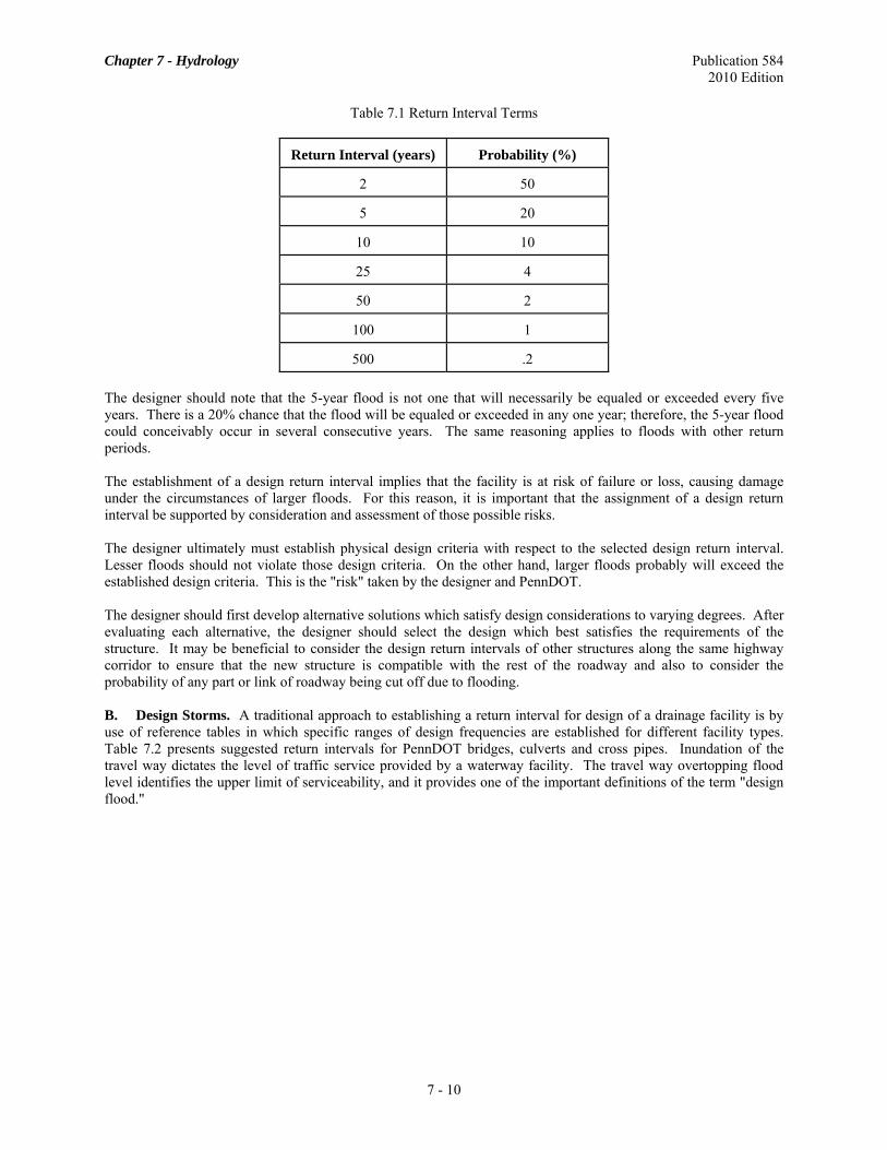
The designer should consider items such as changes in vegetative cover, surface permeability, and constructed drainage systems in estimating future characteristics of the watershed. Q. Climate. Climate changes usually occur over extremely long periods of time such that it is not usually reasonable to consider potential climatic changes during the anticipated life span of the facility. 7.2 DESIGN FREQUENCY A. The Concept of Frequency. As with other natural phenomena, occurrence of flooding is governed by chance. Chance of flooding is described by a statistical analysis of flooding history in the particular watershed of interest. Since it is not economically feasible to design a structure for the maximum possible runoff from a watershed, the designer must choose a return interval appropriate for the structure. The expected return interval for a given flood is defined as the reciprocal of the probability or chance that the flood will be equaled or exceeded in a given year. For example, if a flood has a 20% chance of being equaled or exceeded each year, over a long period of time, the flood will be equaled or exceeded on an average of once every five years. This is called the return period or recurrence interval (RI). Thus exceedance probability equals 100/RI. Table 7.1 lists the probability of occurrence for the standard design return.
Chapter 7 - Hydrology Publication 584 2010 Edition
7 - 10
Table 7.1 Return Interval Terms
Return Interval (years) Probability (%)
2 50
5 20
10 10
25 4
50 2
100 1
500 .2 The designer should note that the 5-year flood is not one that will necessarily be equaled or exceeded every five years. There is a 20% chance that the flood will be equaled or exceeded in any one year; therefore, the 5-year flood could conceivably occur in several consecutive years. The same reasoning applies to floods with other return periods. The establishment of a design return interval implies that the facility is at risk of failure or loss, causing damage under the circumstances of larger floods. For this reason, it is important that the assignment of a design return interval be supported by consideration and assessment of those possible risks. The designer ultimately must establish physical design criteria with respect to the selected design return interval. Lesser floods should not violate those design criteria. On the other hand, larger floods probably will exceed the established design criteria. This is the "risk" taken by the designer and PennDOT. The designer should first develop alternative solutions which satisfy design considerations to varying degrees. After evaluating each alternative, the designer should select the design which best satisfies the requirements of the structure. It may be beneficial to consider the design return intervals of other structures along the same highway corridor to ensure that the new structure is compatible with the rest of the roadway and also to consider the probability of any part or link of roadway being cut off due to flooding. B. Design Storms. A traditional approach to establishing a return interval for design of a drainage facility is by use of reference tables in which specific ranges of design frequencies are established for different facility types. Table 7.2 presents suggested return intervals for PennDOT bridges, culverts and cross pipes. Inundation of the travel way dictates the level of traffic service provided by a waterway facility. The travel way overtopping flood level identifies the upper limit of serviceability, and it provides one of the important definitions of the term "design flood."

Chapter 7 - Hydrology Publication 584 2010 Edition
7 - 11
Table 7.2 Suggested Design Return Intervals (years)
Design Flood Selection Guidelines
Functional Classification Maximum
Exceedance Probability (%)
Minimum Return Period
(years)
Interstate and Limited Access Highways 2 50
Principal Arterial System 2 50
Minor Arterial System 4 25
Rural Collector System, Major 4 25
Other Collector System 10 10
Local Road and Street 10 10 Use of a return period smaller than listed in Table 7.2 must be justified in the hydraulic design analysis for the project and kept with the project's files. Such justification must be based on Consideration of the following kinds of factors:
• Comparison to adjacent roadway sections. • Class of the highway. • Potential flood hazard to property. • Magnitude of damage and risk associated with larger flood events. • Considerations involving right-of-way limitations and constraints imposed by adjacent land use or
development. • Limitations based on the project's scope and budget. • Existing and future level of service. • Future development.
The design flood is assumed to result from the storm with the same return period; therefore, the terms "design flood" and "design storm" have the same meaning. For most highway design projects, it is important to extend the hydrologic and hydraulic analysis to include consideration of floods of magnitudes other than the design floods listed in Table 7.2. These additional floods are referred to collectively as "check floods" and they may include the following kinds of floods:
• The regulatory environmental design flood as specified in 25 PA Code §105.161 (c), §105.191, §105.201, and elsewhere.
• Storms and floods which may be required according to Stormwater Management Plans adopted according to 1978 Act 167 (the Stormwater Management Act).
• The 100-year flood for evaluation of impacts on FEMA's floodplain mapping. • The overtopping flood or greatest flood which must be passed, as discussed in the Federal Aid Policy
Guide, Subchapter G, 23 CFR Parts 650.115 and 650.117. • The specific superflood discussed in Publication 15M, Design Manual, Part 4, Structures, PP Section
7.2.3 for evaluation of the potential effects of scour and evaluation of foundation stability. • The Probable Maximum Precipitation, Probable Maximum Storm, or the Probable Maximum Flood for
projects involving a high risk factor resulting from such considerations as the volume of the impounded water and potential risk of life.
In establishing a design frequency for a drainage facility, the designer (and the Department) takes a risk. The risk is that a flood may occur which is too large for the structure to accommodate. The risk results from the fact that only limited public funding is available for the drainage facility. If funds were unlimited, no risk would be necessary. Use of Table 7.2 only implies but does not quantify the level of risk. For many projects, the potential risks

Chapter 7 - Hydrology Publication 584 2010 Edition
7 - 12
associated with design by frequency selection may be determined to be small such that no further appraisal of risk is necessary. However, if deviation from the suggested design frequencies is contemplated or the potential risks could be significant, the designer should perform a risk assessment. The extent of the assessment should be consistent with the value and importance of the facility (e.g., the consequences). HEC-17, The Design of Encroachments on Flood Plains Using Risk Analysis (FHWA, 1980) and Hydraulic Design of Bridges with Risk Analysis (FHWA, 1980) are suggested references. C. Design by Cost Optimization Using Risk Assessment. The objective of cost optimization is to choose a design return interval which results in a facility that satisfies all the design requirements with the lowest total cost. Structures with lower design return intervals generally have lower construction costs but higher maintenance, repair and replacement costs. A large structure with a high design return interval may have a much larger construction cost yet require less maintenance or repair than a smaller low design return interval structure. The larger structure may last through several lifetimes of the smaller structure. In addition, potential costs of interruption to traffic and other damage may be higher for the smaller structure. The optimal design is one that balances capital costs with operational costs and claims to produce the lowest total cost. Capital costs are those associated with the direct construction of a facility and can be readily estimated. Generally, the higher the design return interval, the higher the capital cost. Operational costs are those associated with maintenance and repair to the facility and costs of any damage incurred by the facility. For the hydraulic design of drainage structures, the primary concern is the potential for flood damage. Risk is defined as the consequences associated with the probability of flooding. For low return interval designs, the probability of flood-related damages and losses may be higher than that associated with higher return interval designs. A risk assessment involves qualitatively evaluating the levels of risk for selected design alternatives. The publication, HEC-17, Design of Encroachments on Flood Plains Using Risk Analysis (FHWA, 1980), provides more extensive detail on this subject. The fact that the example included in HEC-17 refers to a bridge does not imply that risk analysis should be limited to bridges; the same approach is valid for the design of most drainage facilities. Design by cost optimization using risk analysis can be largely subjective and data requirements often are much more extensive than design by return interval selection. The following list provides some examples of situations in which cost optimization may be appropriate:
• Off-system bridge replacements where the existing facility has lower capacity than the suggested design return interval for given hydrologic conditions. Usually, off-system bridges are replaced for reasons other than hydraulic. A risk analysis would help to justify whether a structure larger than the existing structure is needed.
• Where there is a need to determine whether cost of exceeding the 50-year design return interval for a flood plain crossing is justifiable. This may be particularly relevant if 100-year FEMA mapping is involved.
• Justify any design which does fall within the design frequencies suggested in Table 7.2. • Drainage facility for a type that is not addressed in Table 7.2. • Roadway improvements required; existing drainage facilities in good condition but do not meet suggested
design frequency. • Any situation in which the potential risks of damage are high or questionable.
D. Check-Flood Frequencies. Most flood events are of smaller magnitude than the design flood while a few are of greater magnitude. From the standpoint of facility utilization, the designer should strive toward a facility which will operate efficiently for lesser floods, adequately for the design flood, and acceptably for greater floods. For these reasons, it often is important to consider floods of other magnitudes. To define the peak flows for frequencies other than the design frequency, the designer can use the approach of developing a general flood-return interval relation for the subject site. For some drainage facilities, including storm drain systems, the impact of the 100-year flood event should be evaluated depending upon the risk. In some cases, the designer should evaluate a flood event larger than the 100-year flood (super-flood) to ensure the safety of the drainage structure and downstream development. A 500-year flood analysis is required for checking the design of bridge foundations against potential scour failure.
Chapter 7 - Hydrology Publication 584 2010 Edition
7 - 13
There may be instances when the potential for loss of life, disruption of essential services, or excessive economic damages justify a design discharge equal to the Probable Maximum Flood (PMF). The development of the PMF is based upon these steps of estimation:
1. Probable Maximum Precipitation (PMP) from National Weather Service data and generalized charts.
2. Probable Maximum Storm based upon a spatial distribution of the PMP as governed by the following: • Shape. • Orientation. • Movement. • Storm area. • A temporal distribution of precipitation during the storm.
3. PMF based upon hydrograph methods - FHWA Federal Aid Policy 23 CFR 650.
E. Frequencies of Coincidental Occurrence. Where the outfall of a system enters as a tributary of a larger drainage basin, the stage-discharge characteristics of the outfall may depend on the state of the main drainage basin and the probability of flooding events in the two systems may be independent. This is especially common in storm drain systems. For example, a small storm drain system designed for a 5-year return interval discharge may outfall into a major channel associated with a much larger watershed. The two independent events affecting the design are the storm occurring on the small storm drain system and the storm contributing to discharge in the larger watershed. The simultaneous occurrence of two independent events is defined as the product of the probability of the occurrence of each of the individual events. In other words, if the events are independent, the probability of 5-year events occurring on the storm drain and the larger watershed simultaneously is 0.2 * 2 = 0.04 or 4%. This is equivalent to a 25-year frequency. In ordinary hydrologic circumstances, particularly with adjacent watersheds, flood events are not entirely independent. Table 7.3 presents suggested return interval combinations for coincidental occurrence. Each design contains two combinations of frequencies; for instance, a 5-year design with watersheds of one square kilometer (1,000,000 m2), or 0.386 square miles (10,800,000 ft2) and one hectare (10,000 m2, i.e., 100:1), or 2.47 acres (1580 ft2, i.e., 100:1) can employ either of the following:
• A 2-year design on the main stream and a 5-year design on the tributary. • A 5-year design on the main stream and a 2-year design on the tributary.
A structure required that satisfies both return interval combinations is assumed to meet the 5-year design objective. Example:
Determine the 25-year design discharge to be used for a bridge located immediately downstream of the confluence of two streams. Stream A has a contributing drainage area of 100 acres. Stream B has a drainage area of 1,000 acres. The discharges are as follows: Return Period Stream A Stream B
10 yr 300 cfs 2700 cfs 25 yr 450 cfs 3600 cfs
Using the drainage area ratio of 10:1, the table indicates that the 10-, and 25-year event should be combined to determine the combination that governs. 10 yr (A) + 25 yr (B) = 3,900 cfs when routed to structure 10 yr (B) + 25 yr (A) = 3,150 cfs when routed to structure Use the greater of the two calculated numbers to satisfy the design. Note that this number is smaller than that predicted if 25 yr (A) + 25 yr (B) = 4,050 cfs.

Chapter 7 - Hydrology Publication 584 2010 Edition
7 - 14
F. Rainfall versus Flood Frequency. Drainage structures are designed based on some flood frequency. However, certain hydrologic procedures use rainfall and rainfall return interval as the basic input, with the basic assumption that the flood return interval and the rainfall return interval are the same. Depending on antecedent soil moisture conditions and other hydrologic parameters, this may or may not be true. However, for the design of hydraulic structures this is a reasonable assumption.
Table 7.3 Frequencies for Coincidental Occurrence
Area Ratio 2-year design 5-year design
main stream tributary main stream tributary
10,000:1 1 2 1 5 2 1 5 1
1,000:1 1 2 2 5 2 1 5 2
100:1 2 2 2 5 2 2 5 2
10:1 2 2 5 5 2 2 5 5
1:1 2 2 5 5 2 2 5 5
10-year design 25-year design
main stream tributary main stream tributary
10,000:1 1 10 2 25
10 1 25 2
1,000:1 2 10 5 25
10 2 25 5
100:1 5 10 10 25
10 5 25 10
10:1 10 10 10 25 10 10 25 10
1:1 10 10 25 25 10 10 25 25
50-year design 100-year design
main stream tributary main stream tributary
10,000:1 2 50 2 100
50 2 100 2
1,000:1 5 50 10 100
50 5 100 10
100:1 10 50 25 100 50 10 100 25
10:1 25 50 50 100 50 25 100 50
1:1 50 50 100 100 50 50 100 100

Chapter 7 - Hydrology Publication 584 2010 Edition
7 - 15
7.3 HYDROLOGIC METHOD SELECTION A. Overview of Hydrologic Method Selection. Estimating peak discharges of various intervals is one of the most common engineering challenges faced by facility designers. The problem can be divided into two general categories:
• Gaged sites - Limitations on the use of gaged sites is discussed in Section 7.10.C. • Ungaged sites - The site is not near a gaging station and no stream flow record is available. This situation
is very common. This chapter addresses hydrologic procedures that can be used for both categories. This section provides some guidance on selection of hydrologic methods. In general, results from several methods should be compared. The designer should use the discharge that appears to best reflect local project conditions. Averaging of results of several methods is not suggested. In addition, the designer should document reasons supporting the selection of the results. B. Peak Flow Rates versus Hydrographs. Generally, the estimation of peak discharge is adequate for design of conveyance capacity of systems such as storm drains, open channels, culverts and bridges. However, if the design necessitates flood routing (e.g., through storage basins, complex conveyance networks, and pump stations), a flood hydrograph is required. C. Hydrologic Procedures. Countless hydrologic methods are available for estimating peak discharges and runoff hydrographs. The following sections list selected hydrologic methodologies. These methodologies, when properly selected and applied in engineering analyses, will be acceptable to PennDOT, and are preferable over equivalent alternative methodologies. It is not PennDOT's intention to replace the use of sound engineering judgment when any unlisted methodology is determined to be superior; however, use of unlisted methodologies should be coordinated carefully with PennDOT at the earliest possible opportunity during the project development process. The level of accuracy required for a specific hydrologic analysis is a matter of engineering judgment that generally depends on the specific characteristics of each individual project. Factors that tend to control the final accuracy of hydrologic studies include the selection of analytical methods or models and the level of effort invested in data collection and in the application of the method or model. Such factors generally are determined during the early phases of a highway project. With respect to selection of methods or models, this document offers general guidelines regarding selection criteria; however, final decisions regarding the suitability of a particular method for a particular project must be determined by engineering judgment on a case-by-case basis. D. Site Flood History. Discrepancies between any numerical methodology such as HEC-1, TR-55, the rational formula, or a regression method, and the site history should be considered very carefully and explained very thoroughly. Site information such as the performance of an existing structure or the local history of flooding provide important data for corroborating the results of the numerical models used in the hydrologic study, especially if one or more peak water-surface elevations can be determined. When the return periods for a high-water event can be estimated, that event can be used to perform a partial calibration of the hydrologic model. When known events are smaller than the design event, considerable care is required because the estimate of the design peak flow is an extrapolation from the observed historical data. If the watershed has undergone development, construction of flood control structures, reforestation, or other changes since the observed historical events, or if future changes are anticipated, care must be taken to ensure that these factors are accounted for appropriately in the hydrologic study. E. FEMA Studies. If a project site lies within a Federal Emergency Management Agency (FEMA) study area, review the flood discharges reported in the FEMA study and incorporate into the hydrologic analysis. Verify FEMA's flood discharges by an appropriate hydrologic methodology when hydrologic conditions in the basin differ from the conditions described in the FEMA study.

Chapter 7 - Hydrology Publication 584 2010 Edition
7 - 16
For more information about FEMA, contact their web site at www.fema.gov/about/. If FEMA studies are to be used for sizing the waterway structure, then care should be taken to avoid misuse of the information. It should be remembered that the underlying purpose of a FEMA study is very different from a study to design an opening for a waterway structure; therefore, different levels of detail and different methodologies may be appropriate for these two types of studies. Often the FEMA study can be used as a relative comparison, comparing the present condition with the proposed. The hydrologic methods or models used in FEMA studies must be evaluated according to current design guidance and current modeling practices for sizing highway waterway structures. For example, the peak flows in a number of Pennsylvania FEMA studies were based on PSU-III. Use of these peak flows would not be acceptable to the Department because PSU-III was superceded by PSU-IV in 1981. In this case, the results of the FEMA study shall be included in the engineering analysis for comparative purposes. Discrepancies between the results of the FEMA study and the methods selected for the project design shall be carefully analyzed and documented. In all cases, when the site lies within a Federal Insurance Rate Map (FIRM) detailed study area, use of a 100-year discharge that differs from FEMA's for design of a waterway structure requires careful, documented justification that fulfills the review criteria of both the Pennsylvania Department of Environmental Protection (PA DEP) and FEMA. F. 1978 Act 167 Stormwater Management Studies. If the subject drainage basin is part of a Storm Water Management Plan pursuant to 1978 Act 167, review the flood discharges reported in the plan and incorporate into the hydrologic analysis. Verify the flood discharges reported in a storm water management plan by an independent source or methodology if actual conditions in the basin or if map data have changed so that the two studies are based on different hydrologic information. Explain thoroughly the use of flood discharges for design of a waterway structure that differ significantly from the Act 167 discharges. PA DEP's Erosion and Sediment Control Manual, the model Storm Water Management Ordinances for the 1978 Act 167 program, and guidance associated with 25 PA CODE § 102 and § 105 may contain specific limits to the upper limit of applicability of various runoff models. The reader should check the regulations and regulatory guidance for more restrictive requirements. For more information concerning the PA DEP contact their web site at www.depweb.state.pa.us. It should be remembered that the underlying purpose of an Act 167 study is very different from a study to design an opening for a waterway structure; therefore, different levels of detail and different methodologies may be appropriate for these two types of studies. G. Hydrologic Methods and Models. Hydrologic methods are used to determine the various flow rates for waterway structures: design flood, overtopping flood, Q100, Q500, flood-of-record, probable maximum flood, etc. The hydrologic methods and models included in the PennDOT standard H&H toolbox are listed below. Brief statements on the use of the methods are included, as well as information on when the methods should not be used. If a design project does not meet the criteria for using a specific listed method and the method is selected anyway, then justification must be provided for making that selection. For methods that require rainfall depths, such as the rational formula, TR-55, HEC-1, and HEC-HMS, the values should be obtained from Appendix 7A, Field Manual for Pennsylvania Design Rainfall Intensity Charts from NOAA Atlas 14 Version 3 Data. Generally, it may be assumed that rainfall of a given return period produces a flood of the same return period. See Section 7.2.B for specific guidance on selecting magnitudes of design storms. PA DEP has specific limitations to the various hydrologic methods and models that can be used within the state. Also, guidance on the use and limitations of many of the listed methods and models is found in various sections of HDS-2, Highway Hydrology (FHWA, 1996), The Model Drainage Manual (AASHTO, 2005), and the Highway Drainage Guidelines (AASHTO, 2003). H. Analysis of Stream Gage Records. If a design flow rate is being computed for a location on the same "main stem" of a stream within 0.5 to 1.5 times the gage's basin area, stream gage records shall be used to compute design or flood discharges. The hydrologic analysis for the gage should follow the suggestions of Bulletin 17B, Guidelines for Determining Flood Frequency (U.S. Water Resources Council, 1982). The statistical analysis described in Bulletin 17B often is referred to simply as the "WRC" method. Generally, a WRC analysis of a gage record takes precedence over all other hydrologic methods. When a gage record is of short duration, or poor quality, or the

Chapter 7 - Hydrology Publication 584 2010 Edition
7 - 17
results are judged to be inconsistent with field observations or sound engineering judgment, then the analysis of the gage record should be supplemented with other methods. The validity of a gage record should be demonstrated following procedures outlined in Bulletin 17B. Gage records should contain at least 10 years of consecutive peak flow data and they should span at least one wet year and one dry year. If the runoff characteristics of a watershed are changing due to urbanization, for example, then a portion of the record will not be valid. If an invalid portion of a record is used, the results will be biased. The USGS's computer program PEAKFQ performs a standard WRC analysis. The PEAKFQ program and instructions for its use are available from the USGS. The peak flow values computed from a gage record can be
transposed from one location to another if 0.5≤Watershed
g
AA ≤1.5 by scaling the discharge by a ratio of the drainage
areas raised to an exponent. The Peak flow values can be transposed with the following equation: (Equation 7.1)
b
gg AA
⎟⎟⎠
⎞⎜⎜⎝
⎛=
where:
Q = peak discharge, m3/s (cfs) A = basin area above project, ha (ac) Qg = WRC peak discharge at gage, m3/s (cfs) Ag = area of gaged basin, ha (ac) b = drainage area characteristic coefficient from Table 3 in the SIR 2008-
5102 report, Regression Equations for Estimating Flood Flows at Selected Recurrence Intervals for Ungaged Streams in Pennsylvania, (USGS, 2008), for the basin's Flood Flow Region and recurrence interval.
I. Rational Method. The rational method (rational formula) is the suggested hydrologic method for estimating peak flows for drainage areas up to 80 hectares (200 acres) in size. Use of the rational formula on larger drainage areas above this limit requires the use of sound engineering judgment to ensure that reasonable results are obtained. The rational method may be used with caution up to 100 hectares (250 acres) with specific approval by qualified District personnel (typically the District H&H Coordinator). The hydrologic assumptions underlying the rational formula include constant and uniform rainfall over the entire basin with a duration equal to the time of concentration (tc). If a basin has more than one main drainage channel, if the basin is divided so that hydrologic properties are significantly different in one section versus another, if tc > 60 minutes, or if storage is an important factor, then the rational method is not appropriate. For typical roadway drainage problems where all of the conditions discussed in the preceding paragraph are met, the rational method should be applied. When replacing pipes less than 750 mm (30 in) in diameter, the time of concentration (tc) may be reduced to 5 minutes to compute the design discharge. J. Regression Methods. Regional regression equations provide estimates of peak flows at ungaged sites. They are comparatively easy-to-use and they provide relatively reliable and consistent findings when applied by different hydraulic engineers. The three methods listed below, USGS SIR 08-5102, USGS WRIR 00-4189, and PSU-IV, are statistical methods that quantify general regional relationships between peak flows, or other runoff variables, and a watershed's physiographic, hydrologic and meteorologic characteristics. PSU-IV is suggested only as a comparison method unless detailed site history justifies the flows developed using PSU-IV. USGS WRIR 00-4189 has been replaced by the USGS SIR 08-5102 method, but in a few specific scenarios, the USGS WRIR 00-4189 method may be considered as an acceptable method as further discussed in Section 7.3.J.4. The regression processes used to derive the equations in USGS SIR 08-5102, USGS WRIR 00-4189, and PSU-IV tend to smooth the effects of the independent variables on computed peak flow estimates. For basins with atypical hydrologic characteristics, this smoothing effect can be a problem. Atypical characteristics may include steep slopes in the watershed, watersheds with higher length to width ratios, etc. To ensure quality in these hydrologic estimates,

Chapter 7 - Hydrology Publication 584 2010 Edition
7 - 18
it may be prudent to consider comparing the results of USGS SIR 08-5102, USGS WRIR 00-4189, and PSU-IV with the site's history of flooding and/or the results of physically based hydrologic models such as HEC-1. By analyzing and explaining any differences in result from the various methods included in the study, the confidence in the final peak flow estimates can be improved.
1. USGS SIR 08-5102. Regression Equations for Estimating Flood Flows at Selected Recurrence Intervals for Ungaged Streams in Pennsylvania, Scientific Investigations Report (SIR) 08-5102 (USGS, 2008a) is a regression analysis of streamflow data for Pennsylvania drainage basins ranging in size from approximately 259 ha (1.0 mi2) up to approximately 5200 km2
(2000 mi2). USGS SIR 08-5102 was first incorporated into the USGS's National Stream Statistics (NSS) program Version 4.0.b (USGS, 2008b). The program includes regression equations for estimating a typical flood hydrograph for a given recurrence interval as well as other stream low flow statistics. Although the NSS computer program has been incorporated into the Environmental Modeling Research Laboratory's (EMRL) Watershed Modeling System (WMS), WMS 8.1, 8.2 and 8.3 contain NSS version 4.0, which uses the USGS WRIR 00-4189 regression equations. If you are using WMS version 8.3 or older, the hydrologic data must be exported from WMS to use in either a standalone NSS program Version 4.0.b or newer or use the equations from the USGS SIR 08-5102 publication.
2. USGS WRIR 00-4189. Techniques for Estimating Magnitude and Frequency of Peak Flows for Pennsylvania Streams, Water-Resources Investigations Report 00-4189, (USGS, 2000) is a regression analysis of stream flow data for Pennsylvania drainage basins ranging in size from approximately 390 hectares (1.5 mi2) up to approximately 5,200 km2 (2,000 mi2). USGS WRIR 00-4189 rarely is used for basins larger than 650 km2 (250 mi2) because a gaging station normally is available within 0.5 to 1.5 times the basin area.
The equations presented for Region B should not be used if the stream drains a basin with more than 5% urban development. The USGS WRIR 00-4189 regressions equations should not be used for areas less than 390 hectares (1.5 mi2), for streams that drain extensively mined areas or for stream reaches immediately below flood-control reservoirs.
USGS WRIR 00-4189 has been incorporated into the National Flood Frequency (NFF) computer program and the USGS urban regression equations have been included to accommodate developed areas. NFF is available from the USGS's web site for surface water software. NFF has been superseded with the National Stream Statistics (NSS) program which includes the USGS SIR 08-5102 equations as described above.
3. PSU-IV. PSU-IV is a Pennsylvania regional regression method that is based on the Log Pearson III equation. Generally, the PSU-IV regression equations are considered valid for basins from 390 hectares (1.5 mi2) to 390 km2 (150 mi2). PSU-IV is considered to produce good estimates for peak flows in this range; however the PSU-IV model requires caution when being applied to urbanized areas. In urbanized areas in Region 1, the default urban adjustment factor should NOT be applied.
The use of PSU-IV analyses in all urban areas should be based on sound engineering judgment. Urbanized watersheds larger than 39 km2 (15 mi2) require consideration of Stankowski's Urbanization factors in lieu of the default urbanization method in the PSU-IV program or USGS Urban Regression Equation.
Since USGS WRIR 00-4189 is based on data through 1997 and USGS SIR 08-5102 is based on data through 2006, PSU-IV is considered only as a comparison method. PSU-IV can be used to compare estimates from other methods, but should not be used as the final hydrologic method for flow selection unless there is site flooding history that justifies its use. PSU-IV may be used as a comparative method only. 4. Summary of Regression Performance. The two most recent USGS methods (USGS WRIR 00-4189 and USGS SIR 08-5102) were evaluated by PennDOT. In general the USGS SIR 08-5102 method will be the most applicable regression method, but there are some areas of the state that one of the older regression methods may be considered. When compared to observed values (i.e., stream gage analyses), severe under- and over-predictions occur using both USGS methods, and there is no real physiographic or basin characteristic pattern to the results. The USGS regression flows for watersheds with smaller drainage areas (<13 km2 (<5 mi2)) also have inconsistent results. The watersheds where USGS SIR 08-5102 highly over- or under-predicted the gage value are listed in Table 7.4 and shown in Figures 7.2 and 7.3. The observed values were calculated using a Log Pearson III analysis with a weighted skew coefficient, while the weighted values were calculated to minimize period of record bias by computing a predicted flood frequency discharge weighted average of the

Chapter 7 - Hydrology Publication 584 2010 Edition
7 - 19
observed, as well as the USGS SIR 08-5102 computed, using the period of record of the station and the equivalent period of record for the regression equation (USGS, 2008a).
The following procedure is recommended to determine the most appropriate design flows if regression methods are applicable.
5. Recommended Methodology for use of Regression Equations. The USGS SIR 08-5102 regression equations generally perform adequately in predicting flows; however, there are instances where flows may be unrepresentatively high or low in comparison to what one would expect from a stream gage analysis. Therefore, the following set of guidelines should be followed when watershed characteristics are within the limitations of the USGS SIR 08-5102 regression equations.
a. Determine the watershed in which the site is located. b. Determine if the site may be substantially affected by upstream regulation, using USGS SIR 08-5102, Appendix 3 as a guide. c. Determine if the site is in a watershed where USGS SIR 08-5102 may significantly over or under-predict the design event calculated from gage data by referring to Table 7.4 and Figures 7.2 and 7.3. d. Perform calculations using the USGS SIR 08-5102 method to estimate flows. Evaluate the predicted flows in the hydraulic model and compare to local flood history and engineering judgment. e. When the project site is located in one of the two precaution areas mentioned below and the results from USGS SIR 08-5102 are not consistent with the local flood history, it may be necessary to consider other hydrologic methods including the USGS WRIR 00-4189 method or regional gage comparison. Note for the gages/watersheds listed in Table 7.4 and shown in Figures 7.2 and 7.3, consideration should also be given to the number of years of record and quality of data at the gaging station for which the regression flows are being compared.
Precautions for use of the USGS SIR 08-5102 method as a result of PennDOT's evaluation include:
a. USGS SIR 08-5102 results in the watersheds identified in Table 7.4 and Figures 7.2 and 7.3 were particularly different from the gage data and should be closely evaluated for applicability. Some of these watersheds have shown to severely under-predict flows as compared to gage data within the watershed. b. Sites with drainage areas less than <13 km2 (<5 mi2) for both the USGS SIR 08-5102 and USGS WRIR 00-4189 methods.

Chapter 7 - Hydrology Publication 584 2010 Edition
7 - 20
Table 7.4 Gages with the Highest Over- or Under-Predicted USGS SIR 08-5102 Values and Their Watershed Characteristics
Percent Difference from the Weighted
Values
Percent Difference from the Observed
Values
USGS Streamflow
Station Number Station Name
Drainage Area (mi2)
Last Year of Record
Years of Record*
Mean Elevation
Percent Carbonate
Percent Storage
Percent Urban Region
Highest Over-predictions
89 167 1449360 Pohopohco Creek Kresgeville. 49.9 2006 40 1060 0 1.93 7.3 1
35 155 1480800 E. Br. Brandywine Ck. at Downingtown, PA 81.6 1968 11 531 6.72 2.03 9.03 2
81 130 1441000 McMichael Creek near Stroudsburg, PA 65.3 1955 28 952 0.23 3.34 3.17 1
68 118 1447680 Tunkhannock Creek near Long Pond, Pa. 20 2006 40 1,880 0 21.24 0.74 1
68 112 1438300 Vandermark Creek at Milford, Pa. 5.09 2006 45 1,060 0 0.75 5.31 1
Lowest Under-predictions
-61 -71 03008000 Newell Creek near Port Allegany, Pa. 7.79 1978 19 1840 0 0 0.1 3
-64 -70 03049800 Little Pine Creek near Etna, Pa. 5.78 2005 42 1100 0 0 26 4
-57 -68 01638900 White Run near Gettysburg, Pa. 12.5 1980 20 553 0 2.31 8.64 4
-55 -68 01473100 Zacharias Creek near SkipPack, Pa. 7.29 1980 21 322 0 0.06 9.65 2
-53 -67 01479820 Red Clay Creek near Kennett Square, Pa. 28.33 2005 18 371 11.1 1.24 17.6 2
-55 -65 03021410 West Branch French Creek near Lowville, Pa. 52.3 1994 20 1470 0 5.25 1.12 3
-57 -64 01564512 Aughwick Creek near Shirleysburg, Pa. 296 2005 16 1,170 7.03 0.47 0.71 3
-49 -63 01578400 Bowery Run near Quarryville, Pa. 5.98 1981 19 655 25.4 0.98 0.02 2
-50 -63 01553600 EB Chillisquaque Creek near Washingtonville, Pa. 51.5 2005 26 735 6.65 1.14 0.23 1
-45 -62 03100000 Shenango River near Turnersville, Pa. 152 1922 11 1090 0 22.61 5.56 3
-48 -58 01473120 Skippack Creek near Collegeville, Pa. 53.7 1994 29 289 0 0.16 24.7 2
-40 -55 01429500 Dyberry Creek near Honesdale, Pa. 64.6 2005 16 1470 0 3.57 0.21 1
-50 -55 01567500 Bixler Run near Loysville, Pa. 15 2005 52 907 0 0.91 0.23 3
-38 -54 03029000 Clarion River at Ridgway, Pa. 303 2004 12 1910 0 0.93 2.71 3
-44 -54 01516350 Tioga River near Mansfield, Pa. 153 2005 34 1870 0 0.24 1.45 1
-42 -53 01546000 North Bald Eagle Creek at Milesburg, Pa. 119 1934 18 1400 7.47 0.32 0.72 3
-45 -53 01428750 West Branch Lackawaxen River near Aldenville, Pa. 40.6 2006 32 1750 0 1.95 0.28 1
-38 -53 01475530 Cobbs Cr at U.S. Hghwy No. 1 at Philadelphia, Pa. 4.78 2005 18 319 0 0.42 87.7 2
-48 -53 01447500 Lehigh River at Stoddartsville, Pa. 91.7 2006 65 1830 0 14.04 7.47 1
-35 -51 03104760 Harthegig Run near Greenfield, Pa. 2.26 1980 12 1260 0 4.12 2.08 3
-46 -51 03026500 Sevenmile Run near Rasselas, Pa. 7.84 2005 54 2070 0 0 0.16 3
* Years of record used in the USGS SIR 08-5102 analysis primarily consists of systematic period of record and may include historic peak year.

Chapter 7 - Hydrology Publication 584 2010 Edition
7 - 21
Figure 7.2. Watersheds and Gage Numbers with the Highest Over-Prediction from the Observed and Weighted Gage Flows.

Chapter 7 - Hydrology Publication 584 2010 Edition
7 - 22
Figure 7.3. Watersheds and Gage Numbers with the Highest Under-Prediction from the Observed and Weighted Gage Flows.
Chapter 7 - Hydrology Publication 584 2010 Edition
7 - 23
K. HEC-1 & HEC-HMS. HEC-1 & HEC-HMS are generalized hydrologic simulation models that can be used with basins of almost any size and complexity. Use of the Engineering Computing Graphics Laboratory's (ECGL's) Watershed Modeling System (WMS) as an interface to HEC-1 is suggested since it systematizes the computation of the physiographic and hydrologic parameters required by HEC-1. When WMS is used for its graphical user interface to HEC-1, a practical upper limit in the vicinity of 300 to 400 km2 (100 to 150 mi2) is suggested. HEC-1 assumes that the rainfall is spatially uniform over each sub-basin modeled. Soil Conservation Service (SCS) rainfall time distributions, loss methods, dimensionless unit hydrographs, and the lag equations often are used; however, careful consideration must be given to the assumptions and limitations underlying these methods. The SCS developed the curve number method (i.e. the SCS lag equation) for basin sizes less than 800 hectares (2000 acres, 3.1 mi2; NRCS, 1985). The upper limit on basin area for the SCS Loss Method (i.e., Runoff Curve Number) is not well established; however, ~5160 hectares or 52 km2 (1290 acres, 20 mi2) has been suggested. These limitations may be overcome by subdivision of the watershed and appropriate routing. WMS uses USGS Digital Elevation Modules (DEMs) to compute basin geometric parameters. Relatively large data sets are required for, and produced by, WMS for basins spanning more than 8 or 10 DEMs. This may result in a serious degradation of computer performance and may require "overnight" computer runs. The use of HEC-1 by itself may be prudent in these cases. When using WMS in urban areas, care must be taken to ensure that storm water management facilities are incorporated correctly into the model. This will require additional careful modeling and routing. L. WinTR-55 and TR-55. Technical Release 55 (TR-55), Urban Hydrology for Small Watersheds (NRCS, 1986) provides a graphical method for computing peak discharges of drainage basins with areas ranging from 4.0 hectares (10 acres) up to 800 hectares (2000 acres, 3.1 mi2). TR-55 is a segmental method (i.e., flow time is computed by adding the times for the overland, shallow concentrated, and channel segments). TR-55 considers hydrologic parameters such as slope, roughness, losses, rainfall intensity, soil type, land use, and time. Although TR-55 has fewer assumptions than the rational formula, it also assumes that rainfall is uniform over the entire basin. Some hydrologists have stated that TR-55 tends to produce conservatively high estimates of peak flows. TR-55 should be used with caution when structure sizing is highly sensitive to the computed peak flow values. This method must meet the following conditions:
• Basin drained by a single main channel or by multiple channels with times of concentration (tc) within 10% of each other.
• tc between 0.1 and 10 hours. • Storage in the drainage area is ≤ 5% of the basin area and does not affect the time of concentration (i.e.,
storage in the drainage area is not on the main channel in which the tc is being computed and is less than or equal to 5% of the drainage area).
• The watershed can be accurately represented by a single composite curve number. The "Graphical Method" module in the TR-55 computer program and the TR-55 model in WMS are equivalent to the manual graphical method described in the TR-55 report. TR-55 includes a procedure for computing a "rough" synthetic hydrograph, which can be used to size small ponds; however, TR-55 should not be used for flood routing, which would include both channel routing and storage routing. Refer to the TR-55 report for a complete discussion of limitations and assumptions of this methodology. M. EFH-2. EFH-2 determines peak discharge by procedures discussed in Engineering Field Handbook, Chapter 2 (NRCS, 1985). EFH-2 is available online at www.wsi.nrcs.usda.gov/products/W2Q/H&H/Tools_Models/efh2.html. This method is applicable to rural watershed between 0.4047 and 809.4 hectares (1 and 2000 acres), and must meet the following conditions:
• Hydraulic length is between 60.0 and 7,900.8 meters (200 and 26,000 feet).

Chapter 7 - Hydrology Publication 584 2010 Edition
7 - 24
• Average slope is between 0.5 and 64%. • Valley or reservoir routing is not required. • Watershed can be represented accurately by a single composite curve number between 40 and 98. • Urban land uses comprise no more than 10% of the basin.
Refer to the EFH-2 Manual for complete discussion of the methodology and its limitations. 7.4 TIME OF CONCENTRATION A. Overview of Time of Concentration. Several common hydrologic methods require an estimation of the time of concentration. This section provides guidance on ways to estimate time of concentration for use in procedures such as the Rational Method and the SCS runoff curve number methods. The time of concentration (tc) is the time at which all of the watershed begins to contribute to runoff; this is calculated as the time taken for runoff to flow from the most hydraulically remote point of the drainage area to the point under investigation. Various methods can be used to estimate the time of concentration of a watershed. When selecting a method to use in design, it is important to select a method that is appropriate for the flow path. Some methods were developed as lumped parameter methods in that they characterize the time for the entire watershed: the SCS lag equation (Equation 7.2) is an example. Other methods are intended for one segment of the principal flow path and produce a flow velocity that can be used with the length of the segment to compute a travel time (L/V = time). With this method, the time of concentration equals the sum of the travel times on each segment of the principal flow path. Generally, it is reasonable to consider three components of flow which can characterize the progression of runoff along a travel path: sheet flow (overland flow), shallow concentrated flow, and concentrated channel flow or conduit flow. Sheet flow, which is defined mathematically in Section 7.4.C., occurs in the upper reaches of the watershed. Such flow occurs over short distances and at shallow depths prior to the point where topography and surface characteristics cause the flow to concentrate in rills (small depressions that flow intermittently, only when it rains) and swales. Equation 7.3 typically is used to compute the time for this portion of the overland flow. Concentrated flow is runoff that occurs in rills and swales and has depths on the order of 40 to 100 mm (1.58 to 3.94 in). Velocities in open channels usually are determined using the Manning equation to solve for the velocity. There may be a number of possible paths to consider in determining the longest travel time. The designer should identify the flow path along which the longest travel time is likely to occur. This can be a trial-and-error process B. Overland Flow. One way to estimate the overland flow time is to use Publication 13M, Design Manual, Part 2, Highway Design, Chapter 10, Table 10.2.2 to estimate overland flow velocity for a chosen path length. The path length divided by the velocity yields a travel time. A second method is to use the SCS time of concentration equation developed by Mockus in 1961. Equation 7.2 is intended to be the total travel time for the watershed and is considered a lumped parameter equation.
(Equation 7.2) ( ) ( )
5.0
7.08.0 9100067.1KS
CNLtc−
=
where: tc = time of concentration, hr
L = longest hydraulic length from the point of interest to the top of the ridge, m (ft)
CN = SCS runoff curve number, as described in Section 7.4.A K = 2949 (metric), 1900 (U.S. Customary) S = average slope of the watershed in percent

Chapter 7 - Hydrology Publication 584 2010 Edition
Figure 7.4 Velocities for Upland Method of Estimating Time of Concentration, tc (Adapted from National Engineering Handbook, Volume 4 (NEH4), Figure 15.2)
C. Segmental Method.
1. Sheet-flow travel time is a shallow mass of runoff on a plane surface with the depth uniform across the sloping surface. Such flow occurs over relatively short distances, rarely more than ~46 meters (150 feet) (FHWA, 2002). Sheet flow rates are commonly estimated using a version of the kinematic wave equation.
(Equation 7.3) 6.0
4.0 ⎟⎠
⎞⎜⎝
⎛=s
nLiKtt
where: tt = sheet flow travel time, min
K = 6.92 for Metric units or 0.933 for U.S. Customary Units i = rainfall intensity, mm/hr (in/hr) s = surface slope of the flow path, m/m, (ft/ft) n = Manning's n-value (see Table 7.5 for example Manning's n-values) L = longest hydraulic length, m (ft)
Since i depends on Tc and Tc is not initially know, the computation of Tc is an iterative process. An initial estimate of Tc is assumed and used to obtain i from the PDT-IDF curve for the site. The Tc is then computed from Equation 7.3 and used to check the initial value of Tc. If they are not the same, the process is repeated until two successive Tc estimates are the same. Sheet flow can also be determined using Manning's kinematic solution specified in TR-55. 2. The velocity method can be used to estimate travel times for sheet flow, pipe flow, or channel flow. It is based on the travel time for a flow segment as a function of the length and the velocity.
7 - 25

Chapter 7 - Hydrology Publication 584 2010 Edition
7 - 26
(Equation 7.4)
VLTt 60
=
where, L and V have units of meters (feet) and meters/second (feet/second), respectively.
The time of concentration is then equal to the sum of the travel times.
(Equation 7.5)
∑∑==
⎟⎟⎠
⎞⎜⎜⎝
⎛==
k
i i
ik
itic V
LTt11 60
For design conditions that do not involve complex drainage conditions, the designer may use Publication 13M, Design Manual, Part 2, Highway Design, Chapter 10, Table 10.2.2 to estimate the velocities for the various segments. For shallow concentrated flows - After short distances, sheet flow tends to concentrate in rills and gullies of increasing proportions. Such flow usually is referred to as a shallow concentrated flow. The velocity can be estimated with the figures described in this section, or using the relationship between velocity and slope as given below:
(Equation 7.6) V = αkSp
0.5
where: V = velocity, m/s (ft/s) α = 1.0 (metric), 3.28 (U.S. Customary) k = intercept coefficient (see Table 7.6) Sp = slope in percent of the channel or flow
D. Conduit Flow and Open Channel Flow. Pipe or open channel flow time can be estimated from the hydraulic properties of the conduit or channel. Generally it is reasonable to assume uniform flow and employ Manning's Equation with the following considerations. When assuming uniform flow conditions the engineer is assuming that the geometry and slope of the conduit and channel do not vary significantly and that the depth of flow does not vary within the conveyance system (conduit or open channel). If this is not the case, then the methods discussed in the Chapter 8, Open Channels and Chapter 9, Culverts should be used. For open channel flow, consider the uniform flow velocity based on bank full flow conditions. That is, the main channel is flowing full without flow in the overbanks. This assumption avoids the significant iteration associated with other methods which employ rainfall intensity or discharges (since rainfall intensity and discharge are dependent on time of concentration). For conduit flow, in a proposed storm drain system, compute the velocity at uniform depth based on the computed discharge at the upstream stream run. Otherwise, if the conduit is in existence, determine full capacity flow in the conduit and determine the velocity at capacity flow. It may be necessary to compare this velocity later with the velocity calculated during conduit analysis. If there is a significant difference and the conduit is a relatively large component of the total travel path, re-compute the time of concentration using the latter velocity estimate. The coefficients listed are specified on the basis of engineering judgment and do not necessarily reflect the views of research institutions, manufacturers or other governmental agencies.

Chapter 7 - Hydrology Publication 584 2010 Edition
7 - 27
Table 7.5 Roughness Coefficients n-values for Manning's Equation (Pipes and Pavements)
Description Manning's n-value Polyvinyl Chloride (PVC) with smooth Inner Walls 0.010 Corrugated High-Density Polyethylene (HDPE) with Smooth Inner Walls 0.012 Corrugated High-Density Polyethylene (HDPE) with Corrugated Inner Walls 0.015 Concrete Pipe 0.012 Smooth-lined Corrugated Metal Pipe 0.012 Corrugated Plastic Pipe 0.024 Annular Corrugated Steel And Aluminum Alloy Pipe (Plain or polymer coated)
68 mm × 13 mm (2 2/3 in × 1/2 in) Corrugations 75 mm × 25 mm (3 in × 1 in) Corrugations 125 mm × 25 mm (5 in × 1 in) Corrugations 150 mm × 50 mm (6 in × 2 in) Corrugations
0.024 0.027 0.025 0.033
Helically Corrugated Steel And Aluminum Alloy Pipe (Plain or polymer coated) 75 mm × 25 mm (3 in × 1 in), 125 mm × 25 mm (5 in × 1 in),
or 150 mm × 50 mm (6 in × 2 in) Corrugations
0.024 Helically Corrugated Steel And Aluminum Alloy Pipe (Plain or polymer coated) 68 mm × 13 mm (2 2/3 in × 1/2 in) Corrugations
a. Lower Coefficients* 450 mm (18 in) Diameter 600 mm (24 in) Diameter 900 mm (36 in) Diameter 1200 mm (48 in) Diameter 1500 mm (60 in) Diameter or larger b. Higher Coefficients**
0.014 0.016 0.019 0.020 0.021 0.024
Annular or Helically Corrugated Steel or Aluminum Alloy Pipe Arches or Other Non-Circular Metal Conduit (Plain or Polymer coated)
0.024
Vitrified Clay Pipe 0.012 Ductile Iron Pipe 0.013 Asphalt Pavement 0.015 Concrete Pavement 0.014 Grass Medians 0.050 Grass – Residential 0.030 Earth 0.020 Gravel 0.030 Rock 0.035 Cultivated Areas 0.030 - 0.050 Dense Brush 0.070 - 0.140 Heavy Timber (Little undergrowth) 0.100 - 0.150 Heavy Timber (with underbrush) 0.40 Streams: a. Some Grass And Weeds (Little or no brush) b. Dense Growth of Weeds c. Some Weeds (Heavy brush on banks)
0.030 - 0.035 0.035 - 0.050 0.050 - 0.070
Notes:
* Use the lower coefficient if any one of the following conditions apply: a. A storm pipe longer than 20 diameters, which directly or indirectly connects to an inlet or manhole,
located in swales adjacent to shoulders in cut areas, shoulders in cut areas or depressed medians. b. A storm pipe which is specially designed to perform under pressure.
** Use the higher coefficient if any one of the following conditions apply:
a. A storm pipe which directly or indirectly connects to an inlet or manhole located in highway pavement sections or adjacent to curb or concrete median barrier.
b. A storm pipe which is shorter than 20 diameters long. c. A storm pipe which is partly lined helically corrugated metal pipe.

Chapter 7 - Hydrology Publication 584 2010 Edition
In considering each factor more critical, judgment is necessary if it is kept in mind that any condition that causes turbulence and retards flow results in a greater Manning's n-value. Outlet velocity for bituminous paved invert shall be determined based on a 25% reduction in Manning's roughness coefficient, Manning's n-value.
Table 7.6 Intercept Coefficients for Velocity versus Slope Relationship
Land cover (flow regime) k
Forest with heavy ground litter; hay meadow (overland flow) 0.076
Trash fallow or minimum tillage cultivation; contour or strip cropped; woodland (overland flow) 0.152
Short grass pasture (overland flow) 0.213
Cultivated straight row (overland flow) 0.274
Nearly bare and untilled (overland flow) 0.305
Grassed waterway (shallow concentrated flow) 0.457
Unpaved (shallow concentrated flow) 0.491
Paved area; small upland gullies (shallow concentrated flow) 0.619 E. Other Methods for Estimating Travel Time. Other published methods may be used at the designer's discretion subject to the documented limitations of the methods. F. Procedure to Estimate Time of Concentration
1. Divide the flow path into reach lengths along which flow conditions remain reasonably consistent. For natural drainage areas, the upper reaches usually will experience overland or sheet flow which transitions into shallow concentrated flow. If the area is large enough, the lower reaches will experience concentrated flow in swales, ditches, creeks and rivers.
2. For each identified reach length, make an estimate of the travel time and add the individual times to determine the total time. Use a method of estimating time that is appropriate for the flow conditions (see above). If the method results in a velocity, compute the time for component using Equation 7.7.
(Equation 7.7)
n
nn v
Lt60
=
where: tn = travel time over nth reach, min
Ln = length of nth reach along flow path, m (ft) vn = estimated flow velocity for nth reach, m/s (ft/s)
The total time is:
(Equation 7.8)
∑=
=m
nntT
1
where: T = total time along flow path, min
m = number of reaches in flow path n = reach number
7 - 28

Chapter 7 - Hydrology Publication 584 2010 Edition
7 - 29
3. Choose an alternate flow path and repeat steps (1) and (2) as necessary.
4. Select the path which results in the longest time. This is the time of concentration (tc), i.e., tc = T (max).
In some cases, runoff from a portion of the drainage area which is highly impervious may result in a greater peak discharge than would occur if the entire area was considered. In these cases, adjustments can be made to the drainage area and time of concentration by disregarding those areas where flow time is too long to add to the peak discharge. Sometimes it is necessary to estimate several different contributing areas and associated times of concentration to determine the design flow that is critical for a particular application. When designing a drainage system, the overland flow path is not necessarily perpendicular to the contours shown on available mapping. The land may be graded so that swales and streets will intercept the flow and change the time of concentration. Care should be exercised in selecting overland flow paths. 7.5 PEAK DISCHARGE USING THE RATIONAL METHOD A. Introduction to the Rational Method. The Rational Method was first introduced in 1889. Though it often is considered simplistic, it still is deemed to be an appropriate method for estimating peak discharges for small drainage areas of up to 80 hectare (200 acres) in which there is no significant flood storage. B. Assumptions and Applicability of the Rational Method. The Rational Method incorporates the following assumptions:
• The rate of runoff resulting from any constant rainfall intensity is at a maximum when the duration of rainfall is as long as or longer than the time of concentration. That is, if the rainfall intensity is constant, the entire drainage area contributes to the peak discharge when the time of concentration has elapsed. This assumption becomes less valid as the drainage area increases. For large drainage areas, the time of concentration can be so large that constant rainfall intensities for such long periods do not occur and shorter, more intense rainfalls can produce larger peak flows. Additionally, rainfall intensities usually vary during a storm. In semi-arid and arid regions, storm cells are relatively small with extreme intensity variations.
• The frequency of peak discharge is the same as the frequency of the rainfall intensity for the given time of concentration. Frequencies of peak discharges depend on rainfall frequencies, antecedent moisture conditions in the watershed, and the response characteristics of the drainage system. For small, mostly impervious areas, rainfall frequency is the dominant factor. For larger drainage basins, the response characteristics control. For drainage areas with few impervious surfaces (less urban development), antecedent moisture conditions usually govern, especially for rainfall events with a return period of 10 years or less.
• The rainfall intensity is uniformly distributed over the entire drainage area. In reality, rainfall intensity
varies spatially and temporally during a storm. For small areas, the assumption of uniform distribution is reasonable. However, as the drainage area increases, it becomes more likely that the rainfall intensity will vary significantly both in space and time.
• The fraction of rainfall that becomes runoff (C) is independent of rainfall intensity or volume. The assumption is reasonable for impervious areas, such as streets, rooftops, and parking lots. For pervious areas, the fraction of runoff varies with rainfall intensity, accumulated volume of rainfall and antecedent moisture conditions. Thus, the consideration necessary for application of the Rational Method involves the selection of a coefficient that is appropriate for the storm magnitude, soil type, and land use conditions.
By limiting the application of the Rational Method to 80 hectares (200 acres), these assumptions are more likely to be reasonable.

Chapter 7 - Hydrology Publication 584 2010 Edition
Modern drainage practice often includes detention of urban storm runoff to reduce the peak rate of runoff downstream and to improve quality of the storm water runoff. The Rational Method severely limits the evaluation of design alternatives available in urban (and in some instances, rural) drainage design because of its inability to accommodate the presence of storage in the drainage area. When accommodation of any appreciable storage features in the drainage basin is required, runoff hydrograph methods should be employed. C. The Rational Method Equation. The Rational formula estimates the peak rate of runoff at any location in a watershed as a function of the drainage area, runoff coefficient, and mean rainfall intensity for a duration equal to the time of concentration (the time required for water to flow from the most remote point of the basin to the location being analyzed). The rational formula is expressed as Equation 7.9.
(Equation 7.9)
KIACC
Q f=
where: Q = maximum rate of runoff, m3/s (cfs)
C = runoff coefficient as outlined in Section 7.5.E. Cf = runoff coefficient adjustment factor due to return interval I = average rainfall intensity, mm/hr (in/hr) as outlined in Section 7.5.D. A = drainage area, ha (ac) K = 360 (metric), 1 (U.S. Customary)
D. Rainfall Intensity. The rainfall intensity (I) is the average rainfall rate in centimeters per hour (cm/hr) or inches per hour (in/hr) for a specific rainfall duration and a selected frequency. The duration is assumed to be equal to the time of concentration. For drainage areas in Pennsylvania, the rainfall intensity may be determined from the appropriate PDT-Intensity-Duration-Frequency, PDT-IDF, relationships found in Appendix 7A, Field Manual for Pennsylvania Design Rainfall Intensity Charts From NOAA Atlas 14 Version 3 Data. In the Appendix are maps of the different regions depending on the average recurrence interval (ARI) and storm duration. It was found that shorter duration storms had completely different orographic patterns than the longer duration storms, therefore the use of several maps. Rainfall IDF curves for each of the regions are also shown in Appendix 7A, Field Manual for Pennsylvania Design Rainfall Intensity Charts From NOAA Atlas 14 Version 3 Data. As rainfall duration tends towards zero, the rainfall intensity increases. Since the rainfall intensity-duration relationship is calculated by assuming that the duration is equal to the time of concentration, small areas with exceedingly short times of concentration could result in design rainfall intensities that are unrealistically high. To minimize the likelihood that this will occur, the designer should use a minimum time of concentration of 5 minutes. As the duration tends to infinity, the design rainfall tends toward zero. Usually, the area limitation of 80 hectares (200 acres) should result in design rainfall intensities that are not unrealistically low. However, if the estimated time of concentration is extremely long, such as may occur in extremely flat areas, it may be necessary to consider an upper threshold of time (i.e., tc� < 60 minutes) or use a different hydrologic method. There may be instances in which alternate methods of determining rainfall intensity are desired, especially for coordination with other agencies. The designer should take care to ensure that any alternate methods are applicable. E. Runoff Coefficient. The selection of the runoff coefficient (C) tends to be somewhat subjective and varies with the topography, land use, vegetative cover, soil type, and moisture content of the soil at the time the rainfall-producing runoff occurs. In selecting the runoff coefficient, consideration should be given to the future characteristics of the watershed. If land use varies within a watershed, watershed segments must be considered individually and a weighted runoff coefficient, Cw, value can be calculated. Table 7.7 lists suggested ranges of C values for various categories of ground cover. This table is typical of design guides found in civil engineering texts dealing with hydrology. The designer assigns a C value based on what is seen in the watershed with reference to the table. An alternate, systematic approach for developing the runoff coefficient is shown in Table 7.7(a). In this table, which is applicable to rural watersheds only, the watershed is addressed as a series of aspects. For each of four aspects, a
7 - 30

Chapter 7 - Hydrology Publication 584 2010 Edition
7 - 31
systematic assignment of a runoff coefficient "component" is made. Using Equation 7.10, the four assigned components are then added together to form an overall runoff coefficient for the specific watershed segment.
(Equation 7.10) C = Cr + Ci + Cv + Cs
Runoff coefficients, listed in Table 7.7 and Table 7.7(a), and others are applicable for storms of 2-year, 5-year, and 10-year return periods. Higher frequency storms will require modifying the runoff coefficient because infiltration and other abstractions have a proportionally smaller effect on runoff. The designer should adjust the runoff coefficient by the factor Cf as indicated in Table 7.8. Generally, the product of C and Cf should not exceed 1.0.
Table 7.7 Runoff Factors for the Rational Equation
TYPE OF DRAINAGE AREA OR SURFACE RUNOFF FACTOR "C" MINIMUM MAXIMUM
Pavement, concrete or bituminous concrete 0.75 0.95 Pavement, bituminous macadam or surface-treated gravel 0.65 0.80 Pavement, gravel, macadam, etc. 0.25 0.60 Sandy soil, cultivated or light growth 0.15 0.30 Sandy soil, woods or heavy brush 0.15 0.30 Gravel, bare or light growth 0.20 0.40 Gravel, woods or heavy brush 0.15 0.35 Clay soil, bare or light growth 0.35 0.75 Clay soil, woods or heavy growth 0.25 0.60 City business sections 0.60 0.80 Dense residential sections 0.50 0.70 Suburban, normal residential areas 0.35 0.60 Rural areas, parks, golf courses 0.15 0.30
NOTES
1. Higher values are applicable to denser soils and steep slopes. 2. Consideration should be given to future land use changes in the drainage area in selecting the "C" factor.
3. For drainage area containing several different types of ground cover, a weighted value of "C" factor shall be used.
4. In special situations where sinkholes, stripped abandoned mines, etc. exist, careful evaluation shall be given to the selection of a suitable runoff factor with consideration given to possible reclamation of the land in the future.

Chapter 7 - Hydrology Publication 584 2010 Edition
Table 7.7(a) Runoff Coefficient for Rural Watersheds
Slope
extreme high normal low
Relief (Cr)
0.28-0.35 steep, rugged terrain with average slopes above 30%
0.20-0.28 hilly, with average slopes of 10-30%
0.14-0.20 rolling, with average slopes of 5-10%
0.08-0.14 relatively flat land, with average slopes of 0-5%
Soil Infiltration (Ci)
0.12-0.16 no effective soil cover either rock or thin soil mangle of negligible infiltration capacity
0.08-0.12 slow to take up water, clay or shallow loam soils of low infiltration capacity or poorly drained
0.06-0.08 normal; well drained light or medium textured soils, sandy loams
0.04-0.06 deep sand or other soil that takes up water readily, very light well drained soils
Vegetative Cover (Cv)
0.12-0.16 no effective plant cover, bare or very sparse cover
0.08-0.12 poor to fair; clean cultivation, crops or poor natural cover, less than 20% of drainage area over good cover
0.06-0.08 fair to good; about 50% of area in good grassland or woodland, not more than 50% of area in cultivated crops
0.04-0.06 good to excellent; about 90% of drainage area in good grassland, woodland, or equivalent cover
Surface (Cs)
0.10-0.12 negligible; surface depression few and shallow; drainageways steep and small, no marshes
0.08-0.10 well defined system of small drainageways; no ponds or marshes
0.06-0.08 normal; considerable surface depression storage lakes and ponds and marshes
0.04-0.06 much surface storage, drainage system not sharply defined; large flood plain storage or large number of ponds or marshes
The total runoff coefficient based on the four runoff components is: C = Cr + Ci + Cv + Cs
Table 7.8 Runoff Coefficient Adjustment Factors for Rational Method
Recurrence Interval (years) Cf
25 50
100
1.1 1.2
1.25 From The Model Drainage Manual (AASHTO, 2005)
The rational formula now becomes Equation 7.11:
(Equation 7.11)
KIACC
Q f=
F. Procedure for Rational Method. The general procedure for estimating the peak discharge for a watershed using the Rational Method is as follows:
7 - 32

Chapter 7 - Hydrology Publication 584 2010 Edition
1. Determine the watershed area in hectares (acres).
2. With consideration for future characteristics of the watershed, determine the time of concentration as defined in Section 7.4.
3. Assure consistency with the assumptions and limitations for application of the Rational Method.
4. According to the locality in Pennsylvania and the design frequency, extract the rainfall intensity from the appropriate IDF curve.
5. With consideration for future characteristics of the watershed, select or develop appropriate runoff coefficients for the watershed. Where the watershed comprises more than one characteristic, C values for each area segment must be estimated individually. A weighted C value then may be estimated using Equation 7.12.
(Equation 7.12)
CC A
A
n nn
m
nn
m= =
=
∑
∑1
1
where: C = weighted runoff coefficient n = nth sub-area m = number of sub-areas Cn = runoff coefficient for nth sub-area An = nth sub-area size, ha (ac)
The runoff coefficient is dimensionless.
6. Using Equation 7.11, calculate the peak discharge for the watershed for the desired frequency. For frequencies of 2, 5, and 10 years, use Cf = 1. For frequencies 25-year and greater, use Cf from Table 7.8.
G. Example Problem - Rational Method.
1. Problem Statement. The following is an example problem which illustrates the application of the Rational Method to estimate peak discharges. Preliminary estimates of the maximum rate of runoff are needed at the inlet to a culvert for a 10-year and 100-year return period. 2. Site Data. From a topographic map and field survey, the area of the drainage basin upstream from the point in question is found to be 35 hectares (86.5 ac). In addition, the following data were measured:
• Length of sheet flow = 45 m (147.6 ft) • Length of main basin channel = 700 m (2296 ft) • Slope of channel = 0.018 m/m (ft/ft) = 1.8% • Hydraulic radius = 0.6 m (1.97 ft) • Average overland slope = 2.0% • Estimated Roughness • coeff. (n) of channel = 0.090
No shallow-concentrated flow. 3. Determine Runoff Coefficients and n-values From existing land use maps, land use for the drainage basin was estimated to be:
7 - 33

Chapter 7 - Hydrology Publication 584 2010 Edition
• Suburban (average conditions) 80% • Rural, slope 2% 20%
For the residential single-family area:
• Using Table 7.7, the runoff coefficient was estimated for suburban land use: C = 0.45
• Using Table 7.5, the Manning's n-value for grass was estimated n = 0.30
For the rural area:
• Using Table 7.7(a), the runoff coefficient for average conditions was estimated assuming a slope of 0.5%:
C = 0.225 • Using Table 7.5, the Manning's n-value was estimated for woods with light underbrush:
n = 0.400
1 2 3
Land Use Percent of Total
Land Area Runoff Coefficient Product (Area *
Runoff Coefficient) Residential single-family 80 0.45 36.0 Undeveloped 20 0.225 4.5 Total 100 40.5 Weight Runoff Coefficient 0.405
4. Determine Time-of-Concentration (Tc)
Sheet flow - Sheet flow occurs at the head of the basin for the first 150 feet in the residential single-family area.
Note: In the following computations, the i value in the kinematic wave equation is adjusted to the depth of water available as runoff (i.e. C times Cf times the intensity from the PDT-IDF curves). Since i depends on Tc and Tc is not initially know, the computation of Tc is an iterative process. An initial estimate of Tc is assumed and used to obtain i from the PDT-IDF curve for the site. The Tc is then computed from equation 7.3 and used to check the initial value of Tc. If they are not the same, the process is repeated until two successive Tc estimates are the same. For the purpose of this example, the first assumption will be assumed to be the correct one and the iterative process will not be performed.
10-year storm
minutes4.4302.0
45*30.0)22.0*0.1*2.43(
92.692.6 6.0
4.0
6.0
4.0 =⎥⎦
⎤⎢⎣
⎡=⎥⎦
⎤⎢⎣
⎡=S
nLi
Tc
100-year storm
minutes1.3902.0
45*30.0)22.0*25.1*5.71(
92.692.6 6.0
4.0
6.0
4.0 =⎥⎦
⎤⎢⎣
⎡=⎥⎦
⎤⎢⎣
⎡=S
nLi
Tc
Channel Flow
Velocity
mps06.1018.06.0090.011 2/13/22/13/2 === SR
nV
Travel time
7 - 34

Chapter 7 - Hydrology Publication 584 2010 Edition
7 - 35
minutes0.1106.1
70060*
===V
LTch
Total Time of Concentration (Ts + Tch)
10-year: 43.4 + 11.0 = 63.3 minutes (use 63) 100-year: 39.1 + 11.0 = 50.1 minutes (use 50)
5. Determine the rainfall region map. From Appendix 7A, Table 7A.1, determine what the appropriate Rainfall Region Map to be used based on Storm Duration and Frequency.
10-year: 63.3 minutes (use 63) - Map A 100-year: 50.1 minutes (use 50) - Map C
6. Determine the rainfall region. Locate the area of interest on the Pennsylvania Map on the Map that was determined in step 1 (Appendix 7A, Map A – Figure 7A.1, Map C – Figure 7A.3)
10-year: 43.4 + 11.0 = 63.3 minutes (use 63) - Map A – Region 3 100-year: 39.1 + 11.0 = 50.1 minutes (use 50) - Map C – Region 3
7. Determine Intensity (i) A. From the PDT-IDF Curves, determine the Rainfall Intensity in Metric for Region 3 (Appendix 7A, Figure 7A.11(a)).
10 - year = Duration = 63 mins. Region 3 – i = 4.45 cm/hr = 44.5 mm/hr 100- year = Duration = 50 mins. Region 3 – i = 7.37 cm/hr = 73.7 mm/hr
B. From the PDT-IDF Curves, determine the Rainfall Intensity in U.S. Customary (Appendix 7A, Figure 7.11(b)).
10 - year = Duration = 63 mins. Region 3 – i = 1.75 in/hr 100 - year = Duration = 50 mins. Region 3 – i = 2.9 in/hr
8. Determine the Peak Runoff (Q)
A. Determine Peak Runoff in Metric.
10-year
i(63 minutes) = 44.5 mm / hr
smCiAQ
3
25.1360
35*5.44*29.0360
===
100-year
i(50 minutes) = 73.7 mm / h
smCiAC
Q f3
60.2360
35*7.73*29.0*25.1360
===
B. Determine Peak Runoff in U.S. Customary.
10-year
i (63 minutes) = 1.75 in / h cfsacreshrinCiAQ 09.43)(5.86*)/(75.1*29.0 ===
100-year
i (50 minutes) = 2.9 in / h cfsacreshrinCiACQ f 93.90)(5.86*)/(9.2*29.0*25.1 ===
Chapter 7 - Hydrology Publication 584 2010 Edition
7.6 NRCS RUNOFF CURVE NUMBER METHODS A. Introduction to NRCS Methods. The Department uses several runoff determination techniques. A graphical peak discharge method and the dimensionless unit hydrograph method were developed by the U.S. Department of Agriculture, Natural Resource Conservation Service (NRCS), formerly known as the Soil Conservation Service (SCS). TR-55 and EFH-2 also are used by the Department. The graphical peak discharge method and the dimensionless unit hydrograph method will be discussed here. The techniques require basic data similar to that used in the Rational Method. However, the NRCS approach is more sophisticated in that it considers the time distribution of rainfall, initial rainfall losses to interception and depression storage, and an infiltration rate that decreases during the course of a storm. The NRCS methods produce the direct runoff for a storm, either real or fabricated, by subtracting infiltration and other losses from the total rainfall using a method sometimes termed the Runoff Curve Number Method. The primary input variables for the NRCS methods are:
• Drainage area size (A) in square kilometers (square miles). • Time of concentration (tc) in hours. • Weighted runoff curve number (RCN). • Rainfall distribution PDT-IDF Curves. • Total design rainfall (P) in millimeters (in).
The procedures presented here are derived from the National Engineering Handbook, Section 4 (NRCS, 1985) and TR-55, Urban Hydrology for Small Watersheds (NRCS, 1986). B. NRCS Rainfall-Runoff Equation. Equation 7.13 represents a relationship between accumulated rainfall and accumulated runoff. This was derived by the NRCS from experimental plots for numerous soils and vegetative cover conditions. Data for land treatment measures, such as contouring and terracing, from experimental watersheds were included.
(Equation 7.13) ( )( ) SIP
IPR
a
a
+−−
=2
where: R = accumulated direct runoff, mm (in)
P = accumulated rainfall (potential maximum runoff), mm (in) Ia = initial abstraction including surface storage, interception, and infiltration
prior to runoff, mm (in) S = potential maximum retention, mm (in)
The potential maximum retention (S) may be computed as the following:
(Equation 7.14) Metric: U.S. Customary:
25425400−=
RCNS 101000
−=RCN
S
where: RCN = Runoff Curve Number as described in Section 7.6.F.
Equation 7.14 is valid if S < (P - R). Equation 7.14 was developed mainly for small watersheds from recorded storm data that included total rainfall amount in a calendar day, but not its distribution with respect to time. Therefore, this method is appropriate for estimating direct runoff from 24-hour or 1-day storm rainfall. Generally, Ia may be estimated as the following:
(Equation 7.15) Ia = 0.2S
7 - 36

Chapter 7 - Hydrology Publication 584 2010 Edition
which, when substituted in Equation 7.14, gives (Equation 7.16)
( )( )SP
SPR8.0
2.0 2
+−
=
C. Accumulated Rainfall (P). For PennDOT highway drainage design purposes, the accumulated rainfall may be developed from the PDT-IDF Curves for the various regions in the State. D. Rainfall Distribution. The NRCS Type II Rainfall Distribution is commonly used for design studies (TR-55). E. Soil Groups. Soil properties influence the relationship between rainfall and runoff by affecting the rate of infiltration. The NRCS divides soils into four hydrologic soil groups based on infiltration rates: Groups A, B, C, and D.
1. Group A - Soils having a low runoff potential due to high infiltration rates even when saturated, 8.6 to 11.4 mm/hr (0.34 to 0.45 in/hr). These soils consist primarily of deep sands, deep loess, and aggregated silts. 2. Group B - Soils having a moderately low runoff potential due to moderate infiltration rates when saturated, 3.8 mm/hr to 8.6 mm/hr (0.15 to 0.34 in/hr). These soils consist primarily of moderately deep to deep moderately well to well drained soils with moderately fine to moderately coarse textures (shallow loess, sandy loam). 3. Group C - Soils having a moderately high runoff potential due to slow infiltration rates, 1.3 mm/hr to 3.8 mm/hr (0.052 to 0.15 in/hr if saturated). These soils consist primarily of soils in which a layer near the surface impedes the downward movement of water or soils with moderately fine to fine texture (clay loams, shallow sandy loams, soils low in organic content, and soils usually high in clay). 4. Group D - Soils having a high runoff potential due to very slow infiltration rates 1.3 mm/hr (0.052 in/hr). These soils consist primarily of clays with the following characteristics:
• High swelling potential. • Soils with permanently high water tables. • Soils with a claypan or clay layer at or near the surface. • Shallow soils over nearly impervious parent material (soils that swell significantly when wet, heavy
plastic clay, and certain saline soils). Consideration should be given to the effects of urbanization on the natural hydrologic soil group. If heavy equipment can be expected to compact the soil during construction or if grading will mix the surface and subsurface soils, appropriate changes should be made in the soil group selected. F. Runoff Curve Number (RCN). Rainfall infiltration losses primarily are dependent on soil characteristics and land use (surface cover). The NRCS method uses a combination of soil conditions and land use to assign runoff factors known as runoff curve numbers. These represent the runoff potential of an area when the soil is not frozen. The higher the RCN, the higher the runoff potential. Tables 7.9 through 7.12 provide an extensive list of suggested Runoff Curve Numbers. The RCN values assume medial antecedent moisture condition.
(Equation 7.17)
( ) ( )( )IIRCN
IIRCNIRCN058.010
2.4−
=
(Equation 7.18)
)(13.010)(23)(
IIRCNIIRCNIIIRCN
+=
If necessary, the designer should adjust the RCN for wet or dry antecedent moisture conditions. A 5-day period is used as the minimum for estimating antecedent moisture conditions. Antecedent soil moisture conditions also vary during a storm; heavy rain falling on a dry soil can change the soil moisture condition from dry to average to wet during the storm period. Equation 7.17 adjusts values for expected dry soil conditions (antecedent moisture
7 - 37

Chapter 7 - Hydrology Publication 584 2010 Edition
7 - 38
condition I). Use Equation 7.18 to accommodate wet soils (antecedent moisture condition III). Table 7.13 assists the determination of which moisture condition applies.
Table 7.9 Runoff Curve Numbers for Urban Areas
Cover type and hydrologic condition
Average percent
impervious area A B C D
Fully developed urban areas (vegetation established) open space (lawns, parks, golf courses, cemeteries,etc.) Poor condition (grass cover <50%) 68 79 86 89
Fair condition (grass cover 50% to 75%) 49 69 79 84 Good condition (grass cover 50% to 75%) 39 61 74 80
Impervious areas: Paved parking lots, roofs, driveways, etc. (excluding right-of-way) 98 98 98 98
Streets and roads: Paved; curbs and storm drains (excluding right-of-way) 98 98 98 98
Paved; open ditches (including right-of-way) 83 89 92 93 Gravel (including right of way) 76 85 89 91 Dirt (including right of way) 72 82 87 89 Western desert urban areas: Natural desert landscaping (pervious areas only) 63 77 85 88
Artificial desert landscaping (impervious weed barrier, desert shrub with 1- to 2-inch sand or gravel mulch and basin borders)
96 96 96 96
Urban districts: Commercial and business Industrial
85 72
89 81
92 88
94 91
95 93
Residential districts by average lot size: 1/8 acre or less (town houses) 1/4 acre 1/3 acre 1/2 acre 1 acre 2 acres
65 38 30 25 20 12
77 61 57 54 51 46
85 75 72 70 68 65
90 83 81 80 79 77
92 87 86 85 84 82
Developing urban areas Newly graded areas (pervious areas only, no vegetation)
77
86
91
94 • Values in table are for average runoff condition and Ia = 0.2S. • The average percent impervious area shown was used to develop the composite RCN's. Other
assumptions are: (1) impervious areas are directly connected to the drainage system, (2) impervious areas have a RCN of 98, and (3) pervious areas are considered equivalent to open space in good hydrologic condition.

Chapter 7 - Hydrology Publication 584 2010 Edition
7 - 39
Table 7.10 Runoff Curve Numbers for Cultivated Agricultural Land
Cover type Treatment Hydrologic condition A B C D
Fallow Row Crops
Bare soil Crop residue cover (CR) Straight row (SR) SR + CR Contoured (C) C + CR Contoured & terraced (C&T) C&T + CR Small grain SR SR + CR C C + CR C&T C&T + CR Close-seeded SR or broadcast Legumes or C Rotation Meadow C&T
-- Poor Good Poor Good Poor Good Poor Good Poor Good Poor Good Poor Good Poor Good Poor Good Poor Good Poor Good Poor Good Poor Good Poor Good Poor Good Poor Good
77 76 74 72 67 71 64 70 65 69 64 66 62 65 61 65 63 64 60 63 61 62 60 61 59 60 58 66 58 64 55 63 51
86 85 83 81 78 80 75 79 75 78 74 74 71 73 70 76 75 75 72 74 73 73 72 72 70 71 69 77 72 75 69 73 67
91 90 88 88 85 87 82 84 82 83 81 80 78 79 77 84 83 83 80 82 81 81 80 79 78 78 77 85 81 83 78 80 76
94 93 90 91 89 90 85 88 86 87 85 82 81 81 80 88 87 86 84 85 84 84 83 82 81 81 80 89 85 85 83 83 80
• Values in table are for average runoff condition and Ia = 0.2S. • Crop residue cover applies only if residue is on at least 5% of the surface throughout the year. • Hydrologic condition is based on a combination of factors that affect infiltration and runoff, including (1)
density and canopy of vegetative areas, (2) amount of year-round cover, (3) amount of grass or closed-seeded legumes in rotation, (4) percent of residue cover on land surface (good > 20%), and (5) degree of roughness.
• Poor: Factors impair infiltration and tend to increase runoff. • Good: Factors encourage average and better-than-average infiltration and tend to decrease runoff.

Chapter 7 - Hydrology Publication 584 2010 Edition
7 - 40
Table 7.11 Runoff Curve Numbers for Other Agricultural Lands
Cover type Hydrologic condition A B C D
Pasture, grassland, or range-continuous forage for grazing Meadow -- continuous grass, protected from grazing and generally mowed for hay Brush -- brush-weed-grass mixture, with brush the major element Woods -- grass combinations (orchard or tree farm) Woods Farmsteads -- buildings, lanes, driveways, and surrounding lots
Poor Fair Good -- Poor Fair Good Poor Fair Good Poor Fair Good --
68 49 39 30 48 35 30 57 43 32 45 36 30 59
79 69 61 58 67 56 48 73 65 58 66 60 55 74
86 79 74 71 77 70 65 82 76 72 77 73 70 82
89 84 80 78 83 77 73 86 82 79 83 79 77 86
• Values in table are for average runoff condition and Ia = 0.2S. • Pasture: Poor: < 50% ground cover or heavily grazed with no mulch
Fair: 50 to 75% ground cover and not heavily grazed Good: > 75% ground cover and lightly or only occasionally grazed
• Meadow: Poor: < 50% ground cover Fair: 50 to 75% ground cover Good: >75% ground cover
• Woods/grass: RCNs shown were computed for areas with 50% grass (pasture cover). Other combinations of conditions may be computed from RCNs for woods and pasture.
• Woods: Poor: Forest litter, small trees, and brush are destroyed by heavy grazing or regular burning Fair: Woods grazed but not burned, and some forest litter covers the soil Good: Woods protected from grazing, litter and brush adequately cover soil

Chapter 7 - Hydrology Publication 584 2010 Edition
7 - 41
Table 7.12 Runoff Curve Numbers for Arid and Semi-Arid Rangelands
Cover type Hydrologic condition A B C D
Herbaceous -- mixture of grass, weeds, and low-growing brush, with brush the minor element Oak-aspen -- mountain brush mixture of oak brush, aspen, mountain mahogany, bitter brush, maple and other brush Pinyon-juniper -- pinyon, juniper, or both; grass understory Sagebrush with grass understory Desert shrub -- major plants include saltbush, greasewood, creosote-bush, blackbrush, brusage, palo verde, mesquite, and cactus
Poor Fair Good Poor Fair Good Poor Fair Good Poor Fair Good Poor Fair Good
63 55 49
80 71 62 66 48 30 75 58 41 67 51 35 77 72 68
87 81 74 74 57 41 85 73 61 80 63 47 85 81 79
93 89 85 79 63 48 89 80 71 85 70 55 88 86 84
• Values in table are for average runoff condition and Ia = 0.2S. • Hydrologic Condition: Poor: < 30% ground cover (litter, grass, and brush overstory)
Fair: 30% to 70% ground cover Good: > 70% ground cover
• Curve numbers for group A have been developed only for desert shrub
Table 7.13 Rainfall Groups for Antecedent Soil Moisture Conditions During Growing and Dormant Seasons
Antecedent Condition Conditions Description
Growing Season five-day Antecedent Rainfall
Dormant Season five-day Antecedent Rainfall
Dry AMC I An optimum condition of watershed soils, where soils are dry but not to the wilting point, and when satisfactory plowing or cultivation takes place.
Less than 1.39 in (35 mm)
Less than 0.48 in (12 mm)
Average AMC II The average case for annual floods 1.39 to 2.18 in (35 to 55 mm)
0.48 to 1.11 in (12 to 28 mm)
Wet AMC III When a heavy rainfall, or light rainfall and low temperatures, have occurred during the five-days previous to a given storm
Over 2.18 in (55 mm)
Over 1.11 in (28 mm)

Chapter 7 - Hydrology Publication 584 2010 Edition
G. Procedure for NRCS Graphical Peak Discharge (TR-55). This method of peak discharge determination can be used for relatively homogeneous watersheds with a maximum time of concentration of 10 hours (600 minutes). In a similar fashion to the Rational Method, if soils and land use vary, the watershed should be subdivided. Precipitation amounts and distribution can be taken from the PDT-IDF curves for the appropriate regions. The method should not be used for runoff amounts of less than 38 mm (1.50 in) and runoff curve numbers of less than 60. Additionally, the range of curve numbers should be small (say 20%) to reasonably conform with the assumption of homogeneity. The following steps outline the method.
1. Determine the drainage area (A).
2. Determine the soil classification based on runoff potential (Type A, B, C, or D) as described in Section 7.5.E. One approach for a general classification is to determine the soil name and type from NRCS soil maps or reports.
3. Determine the antecedent soil moisture conditions (AMC) as discussed in Section 7.5.F.
4. Classify the hydrologic condition of the soil cover (good, fair or poor). Refer to the footnotes on Tables 7.9 through 7.12.
5. Use Tables 7.9 through 7.13 to determine the Runoff Curve Number (RCN) for the particular soil classification for an AMC II. If appropriate, adjust for AMC I or AMC III using Equations 7.17 and 7.18, respectively. If necessary, determine a weighted value by dividing the sum of the products of the sub-area sizes and RCNs by the total area. This process is similar to the weighting of runoff coefficients in the Rational Method. However, the runoff factors are not directly related.
6. Estimate the watershed time of concentration in hours (tc).
7. Determine the potential maximum storage (S) using Equation 7.14.
8. Determine the initial abstraction (Ia) using Equation 7.15. These are the losses that occur before runoff begins and include depression storage, interception and infiltration. If Ia is greater than P, it is possible that the rainfall event would not produce runoff (which would be unusual for design frequencies). The abstraction equation may need modification or an alternate means of estimating this value may be necessary, although no specific research has been performed to determine such adjustments.
9. Based on the design frequency and a 24-hour duration storm, determine the total rainfall (P) for the location of the watershed.
10. Determine the accumulated direct runoff (R) using Equation 7.16. This value, when multiplied by the watershed area, will indicate the total volume of the rainfall that appears as runoff.
11. Refer to Equation 7.19 and Table 7.15 with the relevant distribution type from Step 9 to determine the unit peak discharge (qu) using time of concentration (tc) and the ratio Ia/P.
(Equation 7.19) ( ) ( )cTCC
cC
u tq log36609.3 21010 +− ×=
where: qu = unit peak discharge, m3/s/km2/mm (cfs/mi2/in) tc = time of concentration, hr
210 ,, CCC = coefficients determined from Table 7.14
7 - 42

Chapter 7 - Hydrology Publication 584 2010 Edition
Table 7.14 Coefficients for Equation 7.19
Rainfall Type Ia/P C0 C1 C2 II 0.1 2.5532 -0.6151 -0.164
0.3 2.4653 -0.6226 -0.1166 0.35 2.419 -0.6159 -0.0882 0.4 2.3641 -0.5986 -0.0562
0.45 2.2924 -0.5701 -0.0228 0.5 2.2028 -0.516 -0.0126
III 0.1 2.4732 -0.5185 -0.1708 0.3 2.3963 -0.512 -0.1325
0.35 2.3548 -0.4974 -0.1199 0.4 2.3073 -0.4654 -0.1109
0.45 2.2488 -0.4131 -0.1151 0.5 2.1777 -0.368 -0.0953
12. With reference to Table 7.15, determine the pond adjustment factor (F). This adjustment is to account for pond or swamp areas within the watershed which do not interfere with the time of concentration flow path.
NOTE: This factor is not intended to replace a hydrograph routing technique where considerable detention storage is present (typically, with surface area of ponding in excess of 5% of the watershed area).
13. Compute the peak discharge (Q) from Equation 7.20.
(Equation 7.20) ARFqQ u=
where: Q = peak discharge, m3/s (cfs)
qu = unit peak discharge, m3/s/km2/mm (cfs/mi2/in) from Step 11 A = drainage area, km2 (mi2) from Step 1 R = runoff volume, mm (in) from Step 10 F = ponding factor from Step 12
Table 7.15 Ponding Adjustment Factor
% Ponded/swamp area Factor (F) 0 1
0.2 0.97 1 0.87 3 0.75 5 0.72
14. Repeat Steps 10 through 13 for other desired frequencies. A detailed description of this method appears in Urban Hydrology for Small Watersheds (NRCS, 1986). H. NRCS (SCS) Dimensionless Unit Hydrograph. In many instances, for highway drainage design, peak discharge methods will suffice for runoff estimation. However, the estimation of runoff hydrographs may be necessary for situations such as detention pond design, reservoir routing, or channel routing, especially for larger areas and those in which watershed conditions cannot be considered homogeneous. Many hydrograph methods are
7 - 43

Chapter 7 - Hydrology Publication 584 2010 Edition
7 - 44
available and not specifically excluded for use by the Department. However, the NRCS Dimensionless Hydrograph Method is incorporated here due to its relative ease of use as well as the relative ease with which variables can be determined. A unit hydrograph represents the time distribution of flow resulting from one millimeter of direct runoff occurring over the watershed in a specified time. The NRCS dimensionless unit hydrograph is plotted in terms of the ratio of time over time to peak. A curvilinear dimensionless unit hydrograph is shown in Figure 7.5. For hand computations, a triangular hydrograph is considered reasonable, as shown in Figure 7.6. The triangular hydrograph is a practical representation of excess runoff with only one rise, one peak, and one recession. Its geometric makeup can be easily described mathematically, which makes it very useful in the processes of estimating discharge rates. The NRCS developed Equation 7.21 to estimate the peak rate of discharge for an increment of runoff.
Figure 7.5 NRCS Dimensionless Curvilinear Unit Hydrograph
q = DISCHARGE AT TIME tqp = PEAK DISCHARGEQa = ACCUMULATED VOLUME
AT TIME t
Tp = TIME FROM BEGINNING OF RISE TO THE PEAK
Q = TOTAL VOLUME
t = A SELECTED TIME
0 1 2 3 40
.1
.2
.3
.4
.5
.6
.7
.8
.9
1.0
5
t / Tp
q/q p
orQ
a/Q
MAS
SC
UR
VE

Chapter 7 - Hydrology Publication 584 2010 Edition
Figure 7.6 Triangular Unit Hydrograph
(Equation 7.21)
pp T
KAqq =
where: qp = peak rate of discharge, m3/s (cfs)
A = area, km2 (mi2) q = depth of storm runoff during time interval = 1 mm (1 in) for unit
hydrograph Tp = time to peak runoff (hours), which is estimated using Equations 7.22 and 7.23 K = 0.208 for metric units and 484 for U.S. Customary Units
7 - 45

Chapter 7 - Hydrology Publication 584 2010 Edition
(Equation 7.22) clag TT 6.0=
(Equation 7.23)
lagp TdT +=2
where: tc = time of concentration, hr
d = duration of unit excess rainfall, hr Equation 7.24 provides an estimate of the duration of unit excess rainfall (d).
(Equation 7.24) d = 0.133 tc
Equation 7.21 can be used to estimate the peak discharge for the unit hydrograph. The shape of the unit hydrograph then can be derived with reference to Figure 7.5. The constant 0.208, or peak rate factor, is valid for the NRCS dimensionless unit hydrograph. Any change in the dimensionless unit hydrograph reflecting a change in the percent of volume under the rising side would cause a corresponding change in the shape factor associated with the triangular hydrograph and therefore a change in the constant 0.208. More detail on the NRCS dimensionless hydrograph method is provided in the National Engineering Handbook, Volume 4 (NRCS, 1985). Dimensionless unit hydrograph characteristics vary with the size, shape, and slope of the tributary drainage area. The most significant characteristics affecting the dimensionless hydrograph shape are the basin lag and the peak discharge (qp) for a given rainfall (see Figure 7.6). Basin lag is the time from the center of mass of rainfall excess to the hydrograph peak. Steep slopes and compact shapes tend to make lag time short and peaks high. Flat slopes and elongated shapes tend to make lag time long and peaks low. I. Procedure for Determining Flood Hydrographs Using the NRCS Dimensionless Unit Hydrograph. The following outline is for design discharges and assumes the area or sub-area is reasonably homogeneous (i.e., the unit hydrograph parameters, hydrologic abstractions, and the rainfall do not vary spatially and are considered constant). That is, the designer has subdivided the watershed into homogeneous areas where these values can be assumed constant. The procedure results in a hydrograph from the direct uncontrolled area. If the watershed has been subdivided, it might be necessary to perform hydrograph channel routing, storage routing, and hydrograph superposition to determine the hydrograph at the outlet of the watershed. Storage routing and channel routing procedures are presented in Sections 7.8 and 7.9.
1. Determine the following parameters:
a. Drainage area or sub-area size, A (km2 or mi2)
b. Time of concentration, tc (hrs) as discussed in Section 7.5.F.
c. Weighted runoff curve number (RCN) as discussed in Section 7.5.F.
d. Total rainfall, P (mm or in), for design and check flood frequencies. Use the 24-hour precipitation.
2. Determine the unit hydrograph variables.
a. Duration of excess rainfall (runoff), d, using Equation 7.23. For convenience, d may be rounded such that the actual duration of precipitation is a whole number times d. For example, if d calculates to be 0.332 hours, for 24-hour precipitation, then 24/0.332 = 72.29; use 72 in which case, d = 24/72 = 0.333 hours (20 mins).
7 - 46

Chapter 7 - Hydrology Publication 584 2010 Edition
b. Time to peak of unit hydrograph (UH), Tp, using Equation 7.22.
c. Compute the peak runoff ordinate, qp, for the UH, using Equation 7.21 and q = 1 mm or 1 in.
d. Using the dimensionless hydrograph (curvilinear, as appears in Figure 7.5, or triangular, as appears in Figure 7.6), develop a table of the unit hydrograph ordinates using time step increments d. That is, at each time n x d, where n is the time step, determine the time ratio (t/Tp).
(Equation 7.25)
pp Tnd
Tt
=⎟⎟⎠
⎞⎜⎜⎝
⎛
e. Find the discharge ratio (q/Qp) at this time ratio and calculate the discharge at this time step as the following equation:
(Equation 7.26)
⎟⎟⎠
⎞⎜⎜⎝
⎛=
pp Q
qqq
f. Use the following to check the area under the resulting hydrograph:
(Equation 7.27) ( )
Aordinateshydrographd ∑×6.3
where A = area of the watershed, km2 (mi2)
The result should be 1.0, reflecting the 1 mm (1 in) of runoff from the entire drainage area. Rounding of the unit duration, d, and the likelihood that Tp will not be an integer multiple of d will often result in an area slightly higher or lower than 1. If so, adjust all the ordinates proportionally until the resulting area is 1.
3. Develop a runoff (excess rainfall) table.
a. Develop a table of accumulated rainfall, P, for the appropriate distribution type and using a time increment of d hours: for each time step (n x d hours), determine the fraction of total rainfall and multiply it by the 24-hour precipitation. (A plot of the resulting values represents a rainfall hyetograph.)
b. On the same table, calculate the accumulated runoff, R, using the estimated RCN and Equations 7.22 and 7.24. If, for any time interval, P - 0.2S < 0, then R = 0.
c. Calculate the increased runoff for each time step as the difference between the current accumulated runoff and the accumulated runoff from the previous time step.
4. Compute the hydrographs resulting from each increment of runoff by multiplying the ordinates of the unit hydrograph by the increment of runoff using the same time step, d. This will result in as many hydrographs as there are increments of runoff, each of which should be displaced by the duration time (d) from the previous hydrograph.
5. At each time step, sum all the runoff values to yield the composite runoff hydrograph. This process step is often termed convolution. This is the resulting hydrograph for the watershed or sub-area. It may serve as an inflow hydrograph for channel or storage routing procedures.
Other superimposition or tabular methods may be used for the convolution process. However, it is expected that computer spreadsheets or programs will be used for large computations and the basic theory remains the same.
7 - 47

Chapter 7 - Hydrology Publication 584 2010 Edition
7 - 48
For complex watersheds, it often is necessary to subdivide the area, develop runoff hydrographs for each sub-area, and perform combinations of flood routing and channel routing. If the appraisal of the effect of storage is required, such as for detention pond design, the resulting hydrographs may be applied to flood-routing techniques such as appear in Section 7.8. Channel routing is discussed in Section 7.9.
7.7 DESIGN RAINFALL HYETOGRAPH METHODS A. Use of the Rainfall Hyetograph. A rainfall hyetograph is a graphical representation of the variation of rainfall depth or intensity with time. Rainfall-runoff hydrograph methods require a description of this variation. It is possible to use actual rain gauge data in rainfall-runoff models if the data are recorded using a small enough time period (such as 15-minute increments). Oftentimes, such data are not readily available. For design, the use of a single measured rainfall event without consideration of other events is not practical since storms vary considerably from event to event and no probability of occurrence would have been established. Two methods discussed here, the NRCS 24-hour Rainfall Distributions and the Balanced Storm Method, are statistically based and appropriate for design. B. NRCS 24-Hour Rainfall Distributions. The NRCS 24-hour distributions are suggested for the design of highway stream crossings (culverts and bridges) where the designer considers it appropriate to employ runoff hydrograph methods. The distributions (Types II and III for Pennsylvania) are presented in Sections 7.8.D. and 7.8.C., respectively. A tabular representation of Types II and III appears in Table 7.16. Table 7.16 represents the cumulative fraction of rainfall with respect to time. The following steps outline the procedure to develop the rainfall hyetograph from the cumulative fraction data.
1. Determine the 24-hour rainfall (P24) for the desired frequency.
2. Establish a time increment (it is useful to use the same time increment as that to be used for hydrograph generation).
3. Establish a table of time and the fraction of rainfall to total 24-hour rainfall by interpolation of Table 7.16 or Figure 7.7 for the appropriate distribution type.
4. Multiply the cumulative fractions by the total 24-hour rainfall to get the cumulative rainfall.
5. Determine the incremental rainfall for each time period by subtracting the cumulative rainfall at the previous time step from the current time step.
A plot of the resulting incremental rainfall versus times represents the rainfall hyetograph.

Chapter 7 - Hydrology Publication 584 2010 Edition
7 - 49
Table 7.16 NRCS 24-Hour Rainfall Distributions
Time (t) hours Fraction of 24-hour rainfall Type II Type III
0 0.000 0.000 2 0.022 0.020 4 0.048 0.043 6 0.080 0.072 7 0.098 0.089 8 0.120 0.115
8.5 0.133 0.130 9 0.147 0.148
9.5 0.163 0.167 9.75 0.172 0.178 10 0.181 0.189
10.5 0.204 0.216 11 0.235 0.250
11.5 0.283 0.298 11.75 0.357 0.339
12 0.663 0.500 12.5 0.735 0.702 13 0.772 0.751
13.5 0.799 0.785 14 0.820 0.811 16 0.880 0.886 20 0.952 0.957 24 1.000 1.000
C. Example of Hyetograph Developed from NRCS 24-Hour Rainfall Distributions (Metric Units). The following is an example of a rainfall hyetograph for a 25-year, 24-hour storm, a 1-hour time increment is used. Total precipitation = 244 mm Distribution type = Type III Table 7.17 presents the calculations. Figure 7.7 shows the resulting hyetograph.
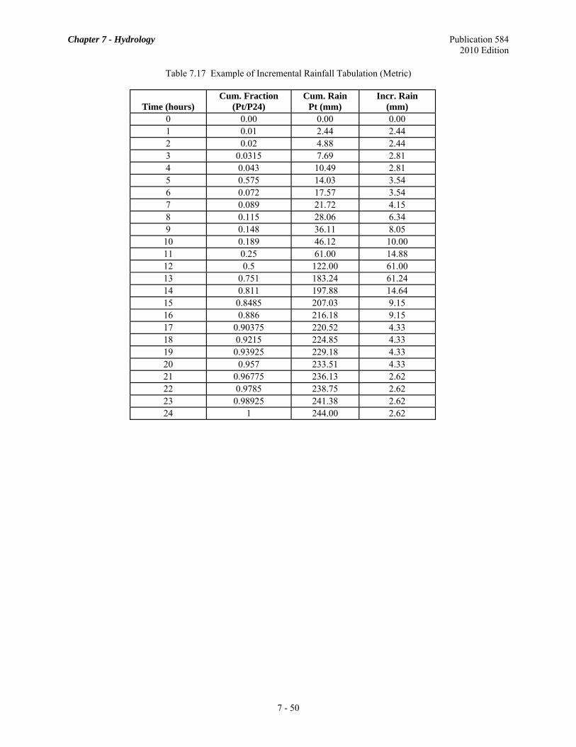
Chapter 7 - Hydrology Publication 584 2010 Edition
7 - 50
Table 7.17 Example of Incremental Rainfall Tabulation (Metric)
Time (hours) Cum. Fraction
(Pt/P24) Cum. Rain
Pt (mm) Incr. Rain
(mm) 0 0.00 0.00 0.00 1 0.01 2.44 2.44 2 0.02 4.88 2.44 3 0.0315 7.69 2.81 4 0.043 10.49 2.81 5 0.575 14.03 3.54 6 0.072 17.57 3.54 7 0.089 21.72 4.15 8 0.115 28.06 6.34 9 0.148 36.11 8.05
10 0.189 46.12 10.00 11 0.25 61.00 14.88 12 0.5 122.00 61.00 13 0.751 183.24 61.24 14 0.811 197.88 14.64 15 0.8485 207.03 9.15 16 0.886 216.18 9.15 17 0.90375 220.52 4.33 18 0.9215 224.85 4.33 19 0.93925 229.18 4.33 20 0.957 233.51 4.33 21 0.96775 236.13 2.62 22 0.9785 238.75 2.62 23 0.98925 241.38 2.62 24 1 244.00 2.62

Chapter 7 - Hydrology Publication 584 2010 Edition
Figure 7.7 Example of Rainfall Hyetograph (Metric)
00 21 3 4 5 6 7 8 9 10 12
Time in hours
Rai
nfal
l Int
ensi
ty in
mm
/hr
11 13 14 15 16 17 18 19 20 2221 23 24
10
20
30
40
50
60
70
For time = 1 hour,
• The cumulative fraction is determined by interpolation of Table 7.16: P1/P24 = 0 + (1 - 0)/(2 - 0) x (0.02 - 0) = 0.01.
• The cumulative rainfall is the product of the cumulative fraction and the total 24-hour rainfall: P1 = 0.01 x 244 = 2.44 mm.
• The incremental rainfall is the difference between the current and preceding cumulative rainfall values: 2.44 - 0 = 2.44 mm.
Repeating the procedure for each time period yields the complete hyetograph ordinates.
7 - 51
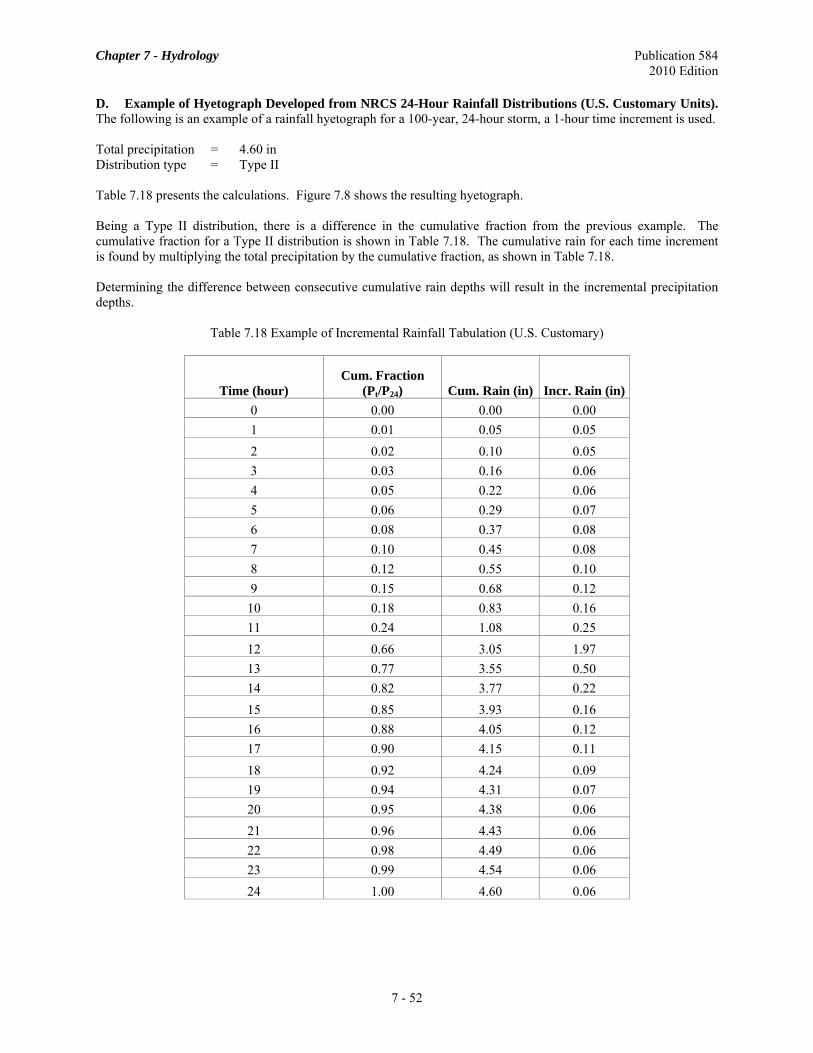
Chapter 7 - Hydrology Publication 584 2010 Edition
7 - 52
D. Example of Hyetograph Developed from NRCS 24-Hour Rainfall Distributions (U.S. Customary Units). The following is an example of a rainfall hyetograph for a 100-year, 24-hour storm, a 1-hour time increment is used. Total precipitation = 4.60 in Distribution type = Type II Table 7.18 presents the calculations. Figure 7.8 shows the resulting hyetograph. Being a Type II distribution, there is a difference in the cumulative fraction from the previous example. The cumulative fraction for a Type II distribution is shown in Table 7.18. The cumulative rain for each time increment is found by multiplying the total precipitation by the cumulative fraction, as shown in Table 7.18. Determining the difference between consecutive cumulative rain depths will result in the incremental precipitation depths.
Table 7.18 Example of Incremental Rainfall Tabulation (U.S. Customary)
Time (hour) Cum. Fraction
(Pt/P24) Cum. Rain (in) Incr. Rain (in) 0 0.00 0.00 0.00 1 0.01 0.05 0.05 2 0.02 0.10 0.05 3 0.03 0.16 0.06 4 0.05 0.22 0.06 5 0.06 0.29 0.07 6 0.08 0.37 0.08 7 0.10 0.45 0.08 8 0.12 0.55 0.10 9 0.15 0.68 0.12
10 0.18 0.83 0.16 11 0.24 1.08 0.25 12 0.66 3.05 1.97 13 0.77 3.55 0.50 14 0.82 3.77 0.22 15 0.85 3.93 0.16 16 0.88 4.05 0.12 17 0.90 4.15 0.11 18 0.92 4.24 0.09 19 0.94 4.31 0.07 20 0.95 4.38 0.06 21 0.96 4.43 0.06 22 0.98 4.49 0.06 23 0.99 4.54 0.06 24 1.00 4.60 0.06

Chapter 7 - Hydrology Publication 584 2010 Edition
Figure 7.8 Example of Rainfall Hyetograph (U.S. Customary)
7 - 53
0.00
0.20
0.40
0.60
0.80
1.00
1.20
1.40
1.60
1.80
2.00
0 1 2 3 4 5 6 7 8 9 10 11 12 13 14 15 16 17 18 19 20 21 22 23 24
Rai
nfal
l Int
ensi
ty (i
n/hr
)
Time (hours)
7.8 STORAGE ROUTING OF FLOOD HYDROGRAPHS A. Flood Routing. Most design situations for Department drainage facilities are accomplished under the general category of steady flow. Steady flow implies no change of discharge with respect to time. As a flood hydrograph approaches and passes through a reservoir or detention facility, the characteristics of unsteady flow become significant. An accounting of inflow and outflow rates per flood time and water storage characteristics must be made. This accounting is accomplished by routing a flood hydrograph through the storage facility. Reservoir or detention pond storage routing is applicable when outflow depends only upon the volume of flood storage. Storage routing techniques are used to do the following:
• Determine peak discharges from watersheds containing reservoirs, flood water detention basins and other flow retardation structures.
• Determine overtopping flood magnitudes. • Evaluate the duration of traffic interruption due to roadway overtopping.
B. Hydrograph Routing Methods. There are several analytical and graphical methods for routing flood hydrographs through reservoirs or other detention facilities. All of the methods require reliable descriptions of three items:
• An inflow runoff hydrograph for the subject flood. • The storage capacity versus water elevation within the retention facility or reservoir. • The performance characteristics of outlet facilities associated with the operation of the reservoir.
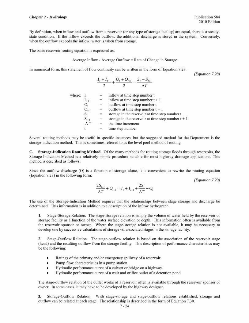
Chapter 7 - Hydrology Publication 584 2010 Edition
By definition, when inflow and outflow from a reservoir (or any type of storage facility) are equal, there is a steady-state condition. If the inflow exceeds the outflow, the additional discharge is stored in the system. Conversely, when the outflow exceeds the inflow, water is taken from storage. The basic reservoir routing equation is expressed as:
Average Inflow - Average Outflow = Rate of Change in Storage In numerical form, this statement of flow continuity can be written in the form of Equation 7.28.
(Equation 7.28)
TSSOOII tttttt
Δ−
=+
++ +++ 111
22
where: It = inflow at time step number t
It+1 = inflow at time step number t + 1 Ot = outflow at time step number t Ot+1 = outflow at time step number t + 1 St = storage in the reservoir at time step number t St+1 = storage in the reservoir at time step number t + 1 Δ T = the time increment t = time step number
Several routing methods may be useful in specific instances, but the suggested method for the Department is the storage-indication method. This is sometimes referred to as the level pool method of routing. C. Storage-Indication Routing Method. Of the many methods for routing storage floods through reservoirs, the Storage-Indication Method is a relatively simple procedure suitable for most highway drainage applications. This method is described as follows. Since the outflow discharge (O) is a function of storage alone, it is convenient to rewrite the routing equation (Equation 7.28) in the following form:
(Equation 7.29)
tt
tttt O
TS
IIOT
S−
Δ++=+
Δ +++ 22
111
The use of the Storage-Indication Method requires that the relationships between stage storage and discharge be determined. This information is in addition to a description of the inflow hydrograph.
1. Stage-Storage Relation. The stage-storage relation is simply the volume of water held by the reservoir or storage facility as a function of the water surface elevation or depth. This information often is available from the reservoir sponsor or owner. Where the stage-storage relation is not available, it may be necessary to develop one by successive calculations of storage vs. associated stages in the storage facility. 2. Stage-Outflow Relation. The stage-outflow relation is based on the association of the reservoir stage (head) and the resulting outflow from the storage facility. This description of performance characteristics may be the following:
• Ratings of the primary and/or emergency spillway of a reservoir. • Pump flow characteristics in a pump station. • Hydraulic performance curve of a culvert or bridge on a highway. • Hydraulic performance curve of a weir and orifice outlet of a detention pond.
The stage-outflow relation of the outlet works of a reservoir often is available through the reservoir sponsor or owner. In some cases, it may have to be developed by the highway designer.
7 - 54
3. Storage-Outflow Relation. With stage-storage and stage-outflow relations established, storage and outflow can be related at each stage. The relationship is described in the form of Equation 7.30.

Chapter 7 - Hydrology Publication 584 2010 Edition
(Equation 7.30)
OTSvsO +⎟⎠⎞
⎜⎝⎛Δ2
This relation can be plotted over the range of anticipated stages. Figure 7.9 illustrates a sample relationship. The form of Equation 7.29 is especially useful because the terms on the left side of the equation are known. With the relation between the outflow and storage determined (Figure 7.9), the ordinates on the outflow hydrograph can be determined directly.
Figure 7.9 Storage-Outflow Relation
Storage Outflow
0
1
2
3
4
5
6
7
0 2.1675 4 .4854 6.9083 9.4199 12.0107 14.6745 17 .4066 20 .2034 25.98 31.9864
2S/T + O
Ou
tflo
w
D. Procedure for Storage-Indication Method. The following steps are used to route an inflow flood runoff hydrograph through a storage system such as a reservoir or detention pond.
1. Acquire or develop a design flood runoff hydrograph.
2. Acquire or develop a stage-storage relation.
3. Acquire or develop a stage-outflow relationship.
4. Develop a storage-outflow relation curve (O vs. 2S/Δ T + O).
5. At time step one (t = 1), assume an initial value for Ot as equal to It. Usually, at time step one, inflow equals zero, so outflow will be zero and 2S1�/T - O1 = 0. Note that to start, t + 1 in the next step is 2.
6. Compute 2St+1/T + Ot+1 using Equation 7.29.
7. From the storage-outflow relation, interpolate to find the value of outflow (Ot+1) at (2St+1)/(T) + Ot+1 from Step 6.
7 - 55

Chapter 7 - Hydrology Publication 584 2010 Edition
8. Determine the value of (2St+1)/(T) - Ot+1 using the relation (2St+1)/(T) -Ot+1 = (2St+1)/(T) + Ot+1 - 2Ot+1.
9. Assign the next time step to the value of t, e.g., for the first run through set t = 2.
10. Repeat Steps 6 through 9 until the outflow value (Ot+1) approaches zero.
11. Plot the inflow and outflow hydrographs. The peak outflow value should always coincide with a point on the receding limb of the inflow hydrograph.
12. Check conservation of mass to help identify success of the process by comparing the inflow volume to the sum of retained and outflow volumes using Equation 7.31.
(Equation 7.31)
∑∑ ×Δ+=×Δ trt OTSIT
where: Sr = volume of runoff completely retained, m3 (ft3) Σ It = sum of inflow hydrograph ordinates, m3 (ft3) ΣOt = sum of outflow hydrograph ordinates, m3 (ft3)
There will be no retention volume if the outflow structure is at the flow line of the pond. A degree of imbalance can be expected due to the discretization process. If the difference is large yet the calculations are correct, reduce the time increment (T), determine the inflow hydrograph values for the new time steps, and repeat the routing process. E. Example of Storage-Indication Method. Table 7.20 presents stage-storage and stage-outflow relations and the computed storage-outflow relation for a detention pond that was designed to reduce peak flows. The following is a sample calculation of the storage-outflow relation (2S/T+O) using a time increment of 15 minutes in Metric Units. At stage = 0.1, S = 904.5 and O = 0.157. Then:
2S/ T + O = (2)(904.5)/(15 x 60) + 0.157 = 2.167 m3/s Δ Table 7.19 presents an inflow hydrograph and routing computations through the detention pond. The following presents sample calculations. When t = 1, I1 = 0, I2 = 0.5, and 2S1/ T-O1 = O. Then: Δ
2S2/ T + O2 = I1 + I2 + 2S1/Δ Δ T - O1 = 0 + 0.5 + 0 = 0.5 m3/s By interpolation (using Table 7.19),
O2 = 0 + (0.5 - 0)(0.1575 - 0) / (2.1675 - 0) = 0.363 m3/s
2S2/ T - O2 = 2S2/Δ Δ T + O2 - 2O2 = 0.5 - (2)(0.0363) = 0.427 m3/s For brevity, the complete outflow ordinates are not shown in Table 7.20. Similarly, in U.S. Customary Units, using Table 7.19: Stage = 0.3 ft, S = 31938 ft3 and O = 5.56 cfs
( )( )O
TS 53.7656.5
60153193822
=+×
=+Δ
cfs
and sample calculations using Table 7.20 are: when t = 1, I1 = 0, I2 = 17.66, and 2S1/Δ T1 - O1 = 0, then:
7 - 56

Chapter 7 - Hydrology Publication 584 2010 Edition
7 - 57
( )
( ) cfsOTSand
cfsOand
cfsOTSIIO
TS
09.15283.1266.172
283.153.76
56.5066.170
66.17066.17022
22
2
11
2122
=−=−Δ
=⎟⎠⎞
⎜⎝⎛−+=
=++=−Δ
++=+Δ
A plot of the resulting outflow hydrograph from the reservoir is superimposed on a plot of the inflow hydrograph (Figure 7.10). It is apparent in this example that the peak flow is attenuated from 141.24 cfs (4.00 m3/s) to 121.75 cfs (3.45 m3/s) by the effects of the available storage in the detention system.
Table 7.19 Stage-Storage-Outflow and Computed Storage-Outflow Relation
Stage Storage Outflow 2S/Δ T+O ft m ft3 m3 cfs m3/s cfs m3/s
0.3 0.1 31938 905 5.56 0.16 76.53 2.17 0.7 0.2 64194 1818 15.73 0.45 158.38 4.49 1.0 0.3 96767 2741 28.89 0.82 243.93 6.91 1.3 0.4 129658 3672 44.49 1.26 332.62 9.42 1.6 0.5 162867 4613 62.17 1.76 424.10 12.01 2.0 0.6 196394 5562 81.72 2.31 518.16 14.67 2.3 0.7 230239 6521 102.99 2.92 614.63 17.41 2.6 0.8 264401 7488 125.82 3.56 713.38 20.20 3.3 1 333680 9450 175.84 4.98 917.35 25.98 3.9 1.2 404229 11448 231.15 6.55 1129.44 31.99

Chapter 7 - Hydrology Publication 584 2010 Edition
Table 7.20 Storage Routing Calculations 1 2 3 4 5 6 7 8
Time step (t)
Time (min)
Inflow I1 + I2 2S/Δ T-O 2S/Δ T+O Outflow (O) Stage
cfs m3/s cfs m3/s cfs m3/s cfs m3/s cfs m3/s ft m 1 0 0.00 0.00 0.00 0.00 0.00 0.00 0.00 0.00 0.00 0.00 2 15 17.66 0.50 17.66 0.50 15.09 0.43 17.66 0.50 1.28 0.04 0.15 0.05 3 30 35.31 1.00 52.97 1.50 58.17 1.65 68.05 1.93 4.94 0.14 0.58 0.18 4 45 52.97 1.50 88.28 2.50 117.95 3.34 146.44 4.15 14.24 0.40 0.89 0.27 5 60 70.62 2.00 123.59 3.50 184.48 5.22 241.53 6.84 28.53 0.81 1.29 0.39 6 75 88.28 2.50 158.90 4.50 250.25 7.09 343.38 9.72 46.57 1.32 1.39 0.42 7 90 105.93 3.00 194.21 5.50 311.65 8.83 444.45 12.59 66.40 1.88 1.78 0.54 8 105 123.59 3.50 229.52 6.50 367.57 10.41 435.23 12.33 86.80 2.46 2.13 0.65 9 120 141.24 4.00 264.83 7.50 418.21 11.84 632.40 17.91 107.10 3.03 2.41 0.74
10 135 129.48 3.67 270.72 7.67 448.59 12.70 688.92 19.51 120.17 3.40 2.79 0.85 11 150 117.69 3.33 247.17 7.00 452.26 12.81 695.76 19.70 121.75 3.45 2.83 0.86 12 165 105.93 3.00 223.62 6.33 441.58 12.51 675.89 19.14 117.16 3.32 2.70 0.82 13 180 94.17 2.67 200.10 5.67 423.19 11.99 641.67 18.17 109.24 3.09 2.48 0.76 14 195 82.38 2.33 176.55 5.00 400.33 11.34 599.74 16.99 99.70 2.82 2.52 0.77 15 210 70.62 2.00 153.00 4.33 374.38 10.60 553.34 15.67 89.48 2.53 2.21 0.67 16 225 58.86 1.67 129.48 3.67 346.35 9.81 503.86 14.27 78.75 2.23 2.20 0.67 17 240 47.07 1.33 105.93 3.00 316.22 8.96 452.28 12.81 68.03 1.93 1.84 0.56 18 255 35.31 1.00 82.38 2.33 284.13 8.05 398.61 11.29 57.24 1.62 1.78 0.54 19 270 23.55 0.67 58.86 1.67 250.00 7.08 342.98 9.71 46.49 1.32 1.39 0.42 20 285 11.76 0.33 35.31 1.00 212.97 6.03 285.31 8.08 36.17 1.02 1.29 0.39 21 300 0.00 0.00 11.76 0.33 172.86 4.90 224.74 6.36 25.94 0.73 1.16 0.36 22 315 0.00 0.00 0.00 0.00 136.95 3.88 172.86 4.90 17.96 0.51 0.77 0.23 23 330 0.00 0.00 0.00 0.00 110.82 3.14 136.95 3.88 13.06 0.37 0.81 0.25 24 345 0.00 0.00 0.00 0.00 91.18 2.58 110.82 3.14 9.82 0.28 0.60 0.18 25 360 0.00 0.00 0.00 0.00 76.42 2.16 91.18 2.58 7.38 0.21 0.45 0.14 26 375 0.00 0.00 0.00 0.00 65.31 1.85 76.42 2.16 5.55 0.16 0.66 0.20 27 390 0.00 0.00 0.00 0.00 55.82 1.58 65.31 1.85 4.75 0.13 0.56 0.17 28 405 0.00 0.00 0.00 0.00 47.71 1.35 55.82 1.58 4.06 0.11 0.48 0.15
7 - 58

Chapter 7 - Hydrology Publication 584 2010 Edition
Figure 7.10 Plot of Inflow and Outflow Hydrographs
7.9 CHANNEL ROUTING OF FLOOD HYDROGRAPHS A. Introduction to Channel Routing. Routing of flood hydrographs by means of channel routing procedures is useful in instances where known hydrographic data are located at a point other than the point of interest. This also is true in those instances where the channel profile or plan is changed in such a way as to alter the natural velocity or channel storage characteristics. Routing analysis estimates the change from the outflow hydrograph to the inflow hydrograph or through a reach. This section describes the Muskingum Method and the Muskingum-Cunge Method, which are lumped flow routing techniques that approximate storage effects in the form of a prism and wedge component (Chow, Maidment, and Mays, 1988). Routing analysis is used to predict the magnitudes, volumes, and temporal patterns of the flow (often a flood wave) as it translates down a channel. The discussion in this section is limited to one-dimensional routing. Thus, at a given instant in time, variation in flow properties is computed from upstream to downstream, but not in the vertical or transverse dimensions of the channel. Almost all flow in river channels is to some extent unsteady; that is, depth, velocity, and flow change with time. The extent of flow variation with time and distance may be such that steady flow computations may be are inappropriate. Some of the applications of unsteady flow analysis include:
• Runoff from precipitation. • Transient flows released from reservoirs during operations for flood control, hydropower generation,
recreation, etc. • Irrigation flows affected by gates, pumps, diversions, etc. • Ocean or lake waves.
7 - 59

Chapter 7 - Hydrology Publication 584 2010 Edition
• Tidal effects in rivers or estuaries. Unsteady flow models based on the complete St. Venant equations, or some simplified form thereof, provide a means for analyzing the flow for engineering applications. The equations are generally written: Continuity Equation:
(Equation 7.32)
0=−∂∂
+∂∂ q
tA
xQ
Moment Equation:
(Equation 7.33)
fo SStV
gxV
gV
xy
−=∂∂
+∂∂
+∂∂ 1
where: Q = discharge, m3/s (cfs) x = distance, m A = cross sectional area, m2 (ft2) t = time, sec q = lateral inflow or outflow, m2/s (ft2/s) Sf = friction slope, m/m (ft/ft) So = channel bed slope, m/m (ft/ft) g = gravitational acceleration, m/s2 (ft/s2)
Routing methods are classified into two categories: hydrologic and hydraulic routing. Both methods attempt to account for volumetric changes in storage as water moves downstream. As such, both of these methods use some form of the continuity equation (Equation 7.32). B. Hydrologic Routing. Hydrologic routing methods combine the continuity equation with some relationship between storage, outflow, and possibly inflow. These relationships can be assumed, empirical, or analytical in nature. An example of such a relationship might be a stage-storage rating, combined with a stage-discharge function such as Manning's equation:
(Equation 7.34) 2
13
21fSAR
nQ =
where R = hydraulic radius, Sf = friction slope, and n = Manning's roughness coefficient, or a simple exponential relationship such as:
(Equation 7.35) Q = aSn
1. Hydraulic Routing. In hydraulic routing analysis, it is intended that the dynamics of the water or flood wave movement be more accurately described than in hydrologic routing. Therefore, hydraulic routing methods combine the continuity equation with a mathematical relationship describing the actual physics of the movement of the water. The momentum equation (Equation 7.34) is the common relationship employed. Open Channel Flow (Henderson, 1966) expressed the momentum equation as:
(Equation 7.36)
tv
gxv
gv
xySS of ∂
∂−
∂∂
−∂∂
−=1
where Sf = the friction slope, So = the bed slope, y = depth, v = velocity, and x = distance longitudinally along the channel. Equations 7.33 and 7.36 are considered to be the full dynamic wave equations or the St. Venant equations. The solution of the full dynamic wave equations requires numerical analysis since no closed form solution of the equations exists.
7 - 60

Chapter 7 - Hydrology Publication 584 2010 Edition
The most common technique used in applying the St. Venant equations is to ignore those terms in the momentum equation which are thought to be negligible, thereby producing simplified hydraulic models. These simplified models are illustrated below: Unsteady non-uniform flow (full momentum equation):
(Equation 7.37)
tv
gxv
gv
xySS of ∂
∂−
∂∂
−∂∂
−=1
Steady non-uniform (quasi-steady model – eliminate time differential):
(Equation 7.38)
xv
gv
xySS of ∂
∂−
∂∂
−=
Diffusion or non-inertial model (eliminate inertial terms):
(Equation 7.39)
xySS of ∂∂
−=
Kinematic model:
(Equation 7.40) of SS =
The following sections are devoted to providing a working knowledge of two of the more popular methods: the Muskingum and the Muskingum-Cunge.
C. Muskingum Method. The Muskingum Method combines a prism component of storage, KO, and a wedge component, KX(I-O), to describe the total storage in the reach as the following equation:
(Equation 7.41) ( )[ ]OXXIKS −+= 1
where: S = total storage, m3 (ft3)
K = a proportionality constant representing the time of travel of a flood wave to traverse the reach(es). Oftentimes, this is set to the average travel time through the reach.
X = a weighting factor describing the backwater storage effects approximated as a wedge
I = inflow, m3/s (cfs) O = outflow, m3/s (cfs)
The value of X depends on the amount of wedge storage; when X = 0 there is no backwater (reservoir type storage) and when X = 0.5 the storage is described as a full wedge. The weighting factor, X, ranges from 0.2 to 0.3 in natural streams. A value of 0.25 is typical. The method is very good when there is not a lot of channel storage and the routing distance is less than 2 km (1.24 miles). Equation 7.42 represents the time rate of change of storage as the following:
(Equation 7.42) ( )[ ] ( )[ ]{ }
TOXXIOxXIK
TSS tttttt
Δ−+−−+
=Δ− +++ 11 111
where: T = time interval usually ranging from 0.3•K to K Δ
t = time step number
7 - 61

Chapter 7 - Hydrology Publication 584 2010 Edition
7 - 62
Applying continuity to Equation 7.42 produces the Muskingum flow routing equation as follows: (Equation 7.43)
tttt OCICICO ⋅+⋅+⋅= ++ 32111 where:
(Equations 7.44 – 7.46)
( )
( )
( )( )1212
122
122
3
2
1
Δ+−Δ−−
=
Δ+−+Δ
=
Δ+−−Δ
=
TXKTXK
C
TXKKXT
C
TXKKXT
C
By definition, the sum of C1, C2 and C3 should be 1. If measured inflow and outflow hydrographs are available, the designer may approximate K and X using Equation 7.47. One calculates X by plotting the numerator on the vertical axis and the denominator on the horizontal axis, and adjusting X until the loop collapses into a single line. The slope of the line equals K.
(Equation 7.47) ( ) ( )[ ]
( ) ( )( )tttt
tttt
OPXIIXOOIIT
K−−+−+−+Δ
=++
++
11
11
15.0
The designer may also approximate K and X using the Muskingum-Cunge Method described in Chow, 1988, or Fread, 1993. D. Example of Muskingum Method. The example shown in Table 7.21 shows a triangular hydrograph routed through three 3280 feet (1000 meter) reaches of channel. The outflow hydrograph for each reach is used as the inflow for the next. The channel has a 'K' of 0.278 hours (1000 seconds) and an X of 0.2.

Chapter 7 - Hydrology Publication 584 2010 Edition
Table 7.21 Channel Routing Using the Muskingum Method
Time Step
Time (s)
Inflow cfs (m3/s)
Outflow cfs (m3/s) Reach 1 Reach 2 Reach 3
1 0 0 (0) 0 (0) 0 0 2 1000 7062 (200) 1629.57 (46.15) 376.05 (10.65) 86.86 (2.46) 3 2000 14124 (400) 7438.05 (210.65) 2680.74 (75.92) 841.08 (23.82) 4 3000 10593 (300) 11766.35 (333.23) 7339.18 (207.85) 3331.15 (94.34) 5 4000 7062 (200) 10048.87 (284.59) 10348.30 (293.07) 7108.61 (201.32) 6 5000 3531 (100) 6936.30 (196.44) 9399.88 (266.21) 9381.87 (265.70) 7 6000 0 (0) 3502.05(99.18) 6712.43 (190.10) 8775.24 (248.52) 8 7000 0 (0) 808.25 (22.89) 3621.04 (102.55) 6475.15 (183.38) 9 8000 0 (0) 186.44(5.28) 1313.89 (37.21) 3747.45 (106.13)
10 9000 0 (0) 43.08 (1.22) 413.48 (11.71) 1667.69 (47.23) 11 10000 0 (0) 9.89 (0.28) 120.76 (3.42) 635.58 (18.00) 12 11000 0 (0) 2.12 (0.06) 33.90 (0.96) 219.63 (6.22) 13 12000 0 (0) 0.35 (0.01) 9.18 (0.26) 70.97 (2.01) 14 13000 0 (0) 0.00 2.47 (0.07) 21.89 (0.62) 15 14000 0 (0) 0.00 0.71 (0.02) 6.36 (0.18) 16 15000 0 (0) 0.00 0.00 1.77 (0.05) 17 16000 0 (0) 0.00 0.00 0.71 (0.02) 18 17000 0 (0) 0.00 0.00 0.00
Using Equations 7.44, 7.45, and 7.46 with a time increment of 1000 s:
( )( )( )( )
( )( )( )( )
( )( )( )( ) 23077.0
10002.011000210002.0110002
53846.010002.0110002
2.0100021000
23077.010002.0110002
2.0100021000
3
2
1
=+−−−
=
=+−
+=
=+−
−=
C
C
C
Check:
C1 + C2 + C3 = 0.23077 + 0.23077 + 0.53846 = 1 For time step two, (t = 2), first reach:
O2 = (0.23077)(7062) + (0.53846)(0) + (0.23077)(0) = 1629.70 cfs O2 = (0.23077)(200) + (0.53846)(0) + (0.23077)(0) = 46.15 m3/s
For time step three, (t = 3):
O3 = (0.23077)(14124) + (0.53846)(7062) + (0.23077)(1630) = 7438.16 cfs O3 = (0.23077)(400) + (0.53846)(200) + (0.23077)(46.15) = 210.65 m3/s
Repeat the process until the outflow hydrograph is complete. The outflow hydrograph from reach 1 becomes the inflow hydrograph for reach 2 and the process is repeated for reaches 2 and 3. Since the outflow hydrograph represents a displacement in distance as well as time, the peak outflow does not coincide with the receding limb of the inflow hydrograph.
7 - 63

Chapter 7 - Hydrology Publication 584 2010 Edition
E. Muskingum-Cunge Method.
1. Description of Method. "On the Subject of a Flood Propagation Computation Method (Muskingum Method)" (Cunge, 1969) states that the Muskingum method is essentially a finite difference form of the St. Venant equations after neglecting the inertia terms. This neglecting of the inertia terms implies the Muskingum method is of a kinematic nature. "On the Subject of a Flood Propagation Computation Method (Muskingum Method)" (Cunge, 1969) introduced alternative methods for calculating the routing coefficients in the Muskingum method, which effectively produces results based on diffusion analogy, rather than the kinematic nature of the basic Muskingum method. This method is known as the Muskingum-Cunge routing method. The Muskingum-Cunge routing method produces good results for many applications without the computational problems associated with fully dynamic routing models. The method is non-linear in that routing coefficients, as a function of flow properties, are recalculated with each time step. The method requires input values of representative channel cross section, slope and roughness for the routing reach. 2. Assumptions. Use of the method requires the assumption that backwater effects are negligible and that channel geometry, slope and roughness data are adequate to characterize the hydraulics over the reach represented by a given cross section. 3. Limitations. The Muskingum-Cunge method combines the continuity equation and the diffusion form of the momentum equation. As such it accounts for flood wave attenuation, but not for reverse flow or backwater effects. The Muskingum-Cunge technique is not well suited for fast rising hydrographs such as those encountered in dam break situations. 4. Data Requirements. Muskingum-Cunge routing requires representative cross section geometry, slope and roughness for each reach simulated. 5. Development of Equations. The Muskingum-Cunge formulation is similar to the Muskingum formulation. The Muskingum-Cunge derivation begins with the continuity equation and includes the diffusion form of the momentum equation. These equations are combined and linearized, producing the following convective diffusion equation (Miller and Cunge, 1975).
(Equation 7.48)
xcqxQd
xQc
tQ
+∂
=∂∂
+∂∂
2
2
μ
where: Q = discharge, m3/s (cfs)
t = time, sec x = distance along channel, m (ft) qx = lateral inflow, m2/s (ft2/s) c = wave celerity, m/s (ft/s) μ = hydraulic diffusivity, m2/s (ft2/s)
The wave celerity is defined as follows:
(Equation 7.49)
dAdQc =
and the hydraulic diffusivity is defined:
(Equation 7.50)
oBSQ
2=μ
where S0 is the bed slope and B is the top width of the flow area.
7 - 64

Chapter 7 - Hydrology Publication 584 2010 Edition
The solution of the Muskingum-Cunge procedure is accomplished by discretizing the equations on an x-t plane. The equation applied to the discretized plane, allowing for lateral inflow, is as follows:
(Equation 7.51)
Lnj
nj
nj
nj QCQCQCQCQ 413
121
11 +++= +
+++
where the coefficients are defined to be:
(Equations 7.52 - 7.55)
( )
( )
( )
( )
( )12
2
12
12
12
2
12
2
4
3
2
1
−+Δ
⎟⎠⎞
⎜⎝⎛
=
−+Δ
Δ−−
=
−+Δ
−Δ
=
−+Δ
+Δ
=
XK
tKBt
C
XK
tK
tXC
XK
t
XK
t
C
XK
t
XK
t
C
6. Use and Estimation of Parameters. In the Muskingum-Cunge method, the travel time parameter, K, is calculated using the reach length, x, and the wave celerity, c, as:
(Equation 7.56)
cxK Δ
=
and the parameter X is calculated as a function of the flow properties:
(Equation 7.57)
⎟⎟⎠
⎞⎜⎜⎝
⎛Δ
−=xcBS
QXo
121
The parameters required to apply Muskingum-Cunge routing are channel cross section geometry (either as a regular trapezoid or rectangle, or as an eight-point cross section), channel slope, roughness, and the length of the channel element represented by these parameters. One must take particular care when choosing the computation interval, since the computation interval must not be longer than the time it takes for the wave to travel the reach distance. If the wave travels faster than the time step, the computation will not indicate the proper storage.
7 - 65
Chapter 7 - Hydrology Publication 584 2010 Edition
7.10 STATISTICAL ANALYSIS OF STREAM GAGE DATA A. Introduction to Statistical Analysis of Stream Gage Data. The estimation of peak discharges of various recurrence intervals is one of the most common problems faced by engineers when designing for highway drainage structures. The problem can be divided into three categories:
1. If the site is at a gaging station, and the streamflow record is fairly complete (no missing data) and of sufficient length then flood frequency analysis using the log-Pearson Type III distribution will be used to determine the peak flows for the various return periods desired.
2. If there is no gage at the site, but there is a gage on the same stream that can be transposed (the gage's
data can be transposed if 0.5≤Watershed
g
AA
≤1.5), then the gaged data will be transposed to the site using an area
relationship given in Section 7.3.H. or based on the method outlined in USGS SIR 08-5102. 3. If there is no gage on the stream and the watershed characteristics are within the bounds of the USGS SIR 08-5102 and/or USGS WRIR 00-4189 procedure, then USGS SIR 08-5102 and/or USGS WRIR 00-4189 will be applied to determine the peak flows for the various return periods desired based on the regression procedure discussed in Section 7.3.J.5. If USGS SIR 08-5102 and/or USGS WRIR 00-4189 is not appropriate for the specific site then a hydrograph model such as HEC-1 should be used to determine the peak discharges.
Bulletin 17B, Guidelines for Determining Flood Flow Frequency (U.S. Water Resources Council, 1982) is a guide that describes the data and procedures for computing flood flow frequency curves where stream gaging records of sufficient length are available. The Bulletin was intended for use for analyzing records of annual flood peak discharges, including both systematic records and historic data. There are numerous statistical distribution methods for establishing peak discharge versus frequency relations. The log Pearson Type III statistical distribution method has gained the most widespread acceptance and is suggested by Bulletin 17B. An outline of this method follows; however, the designer is not limited to using only this method, especially if the resulting discharge frequency relation does not seem to fit the data adequately (e.g. other methods have a smaller standard of error). B. Sources of Stream Gage Records. Generally, for Department application, the designer will need to acquire a record of the annual peak flows for the appropriate gaging station. The following sources provide stream gage records:
• U.S. Geological Survey Water Resources Data - Pennsylvania, Surface Water. These are prepared annually and contain records for one water year per publication.
• International Boundary and Water Commission Water Bulletins. • USGS database WATSTORE. • INTERNET file transfer protocol (ftp) sites. • Compact Disk Read Only Memory (various vendors).
The designer should ensure acquisition of the most recent published records. C. Applicability and Limitations. For highway drainage purposes, a statistical analysis of stream gage data is applied only in those instances where there is adequate data from stream gaging stations. Bulletin 17B states that stream gage records must contain a minimum of 10 years of data to warrant a statistical analysis (see also Section 7.3.H). Water-Quality Conditions During Low Flow in the Lower Youghiogheny River Basin, Pennsylvania, October 5-7, 1998 (USGS, 1998) contains a procedure for computing weighted peak flows and equivalent periods of record for stream gages. This procedure can be used to extend short gage records that meet the minimum requirement for number of years. In some cases, a site needing a design peak discharge will be located on the same stream and near to the location of an active or discontinued stream gaging station with an adequate length of record. A list of all the active and discontinued gaging stations in the state can be obtained from the USGS in Harrisburg, PA. Having determined that a suitable stream gage record exists, it is necessary to determine if any structures or organization may be affecting the peak discharges at the design site. The period of record for the gaging station's 7 - 66

Chapter 7 - Hydrology Publication 584 2010 Edition
annual-peak discharges should represent the same or similar basin conditions as that of the design state. A time series analysis may be required to determine if there is an impact caused by the upstream structure. Therefore, any gaged peak discharges not representing the basin conditions for the design site should be excluded from the analysis. The most typical factors affecting peak discharges are urbanization and regulation by reservoirs. Densities of impervious cover less than 10% of the watershed area generally do not affect peak discharges. The existence in the watershed of a major reservoir or many small reservoirs or flood control structures can greatly affect the runoff characteristics. The length of record should be adjusted to include only those records that have been collected subsequent to the impoundment of water by reservoirs and subsequent to any major urbanization. If the resulting records then become too short as defined above, do not use the method outlined in Section 7.10.D. D. Log-Pearson Type III Distribution. The log-Pearson Type III method for the statistical analysis of gaged flood data is applicable to just about any series of natural floods. Three statistical moments are involved in the analysis:
• The mean is approximately equal to the logarithm of the 2-year peak discharge. • The standard deviation, which is the second moment of the logarithm of the discharges, can be compared
to the slope of the plotted curve. (Although, with the consideration of the third moment, skew, there is no single slope to the curve.)
• The skew (the third moment of the logarithm of the peak discharges) represents the form of curvature to the plotted curve.
On log-probability paper, a negative skew of the flood-frequency curve is concave downward and for a positive skew, the curve is concave upward. If the skew is zero, the plotted relation forms a straight line, the distribution is defined as normal, and the standard deviation becomes the slope of that straight line. Because of these tendencies, the significance of the skew becomes especially important in the estimation of floods based upon extrapolated curves (i.e., for a large positive skew with limited years of record, the 100-year return period flood peak may be over predicted). Because flooding is often erratic in Pennsylvania, a series of observed floods may include annual peak discharge rates which do not seem to belong to the population of the series. The values may be extremely large or extremely small with respect to the rest of the series of observations. Such values may be "outliers" which possibly should be excluded from the set of data to be analyzed. Additionally, adjustment can be made to incorporate historical data. Caution should be exercised when dealing with high outliers and if at all possible the record should be extended by incorporating historical data (see Bulletin 17B). To make the analysis of the Log-Pearson Type III method easier, the computer program PEAKFQ is available from the USGS. Section 7.10.E. outlines the procedure for the Log-Pearson Type III method for understanding and reference only. E. Log-Pearson Type III Analysis Procedure.
1. Acquire and assess annual peak discharge record. There are instances when the annual peak discharge data may be suspect. For projects containing stream gage data affected by outliers, coordination with the USGS is suggested to obtain the final design peak flows. The record should comprise only one discharge (maximum) per year. Note that the USGS water year is October through September.
2. Calculate the logarithm of the base 10 for each discharge value.
3. Calculate the statistics using Equations 7.58, 7.59, and 7.60.
(Equation 7.58)
NX
QL∑=
(Equation 7.59)
7 - 67

Chapter 7 - Hydrology Publication 584 2010 Edition
( ) 21
2
1
2
⎪⎭
⎪⎬⎫
⎪⎩
⎪⎨⎧
−
∑−= ∑
NX
S N
x
L
(Equation 7.60) ( ) ( )( ) ( )
( )( ) 3
3232
2123
LS SNNN
XXXNXNG
−−
+−= ∑∑∑∑
where: LQ = mean of the logarithms of the annual peak discharges, m3/s (cfs)
N = number of observations X = logarithm of the annual peak discharge, m3/s (cfs) SL = standard deviation of the logarithms of the annual peak discharge, m3/s
(cfs) GS = coefficient of skew of log values (station skew)
4. For each frequency (typically 2 through 100 year), calculate the logarithm of the discharge using Equation 7.61.
(Equation 7.61) LL KSQQ +=log
where: Q = flood magnitude, m3/s (cfs)
K = a frequency factor for a particular return period and coefficient of skew
5. Plot discharge versus frequency on standard log probability paper.
6. Consider adjusting the calculations to accommodate a weighted skew and outliers as discussed in Sections 7.10.F. and 7.10.G., respectively.
F. Skew. There are three methods for determining the value of the skew coefficient for the log Pearson Type III curve fit.
1. The station skew is calculated directly from the gage data using Equation 7.60. This value may not represent the skew of the parent population accurately if the period of record is short or if there are extreme events in the period of record.
2. Figure 7.11 shows the value of generalized skew coefficients across Pennsylvania. The designer may use the generalized skew coefficient identified by the map based upon the project location.
3. The designer may compute a weighted skew. Refer to Bulletin 17B for the method. (Note: The mean square error for the generalized skew is 0.35 which replaces the value of 0.55 presented in Bulletin 17B.)
It is preferable to use a weighted skew as described in Bulletin 17B for all flood peak estimates. The weighted value and can also be obtained from the USGS in Harrisburg, PA. G. Accommodating Outliers in the Data. The distribution of all the annual and historical peak discharges determines the shape of the frequency curve, and thus the design-peak discharges. For a Log-Pearson Type III analysis, the distribution of the high peak discharges affects the shape of the curve and the value of the low peak discharges. In most peak-stream flow frequency analyses, the larger recurrence-interval peaks are needed more often than those for the lower recurrence intervals. Most design peaks, for example, are based on 10-year, 25-year, 50-year, or 100-year recurrence intervals rather than 2-year or 5-year intervals. Therefore, it would be more desirable for the shape of the frequency curve to be based on the distribution of the larger peaks.
7 - 68
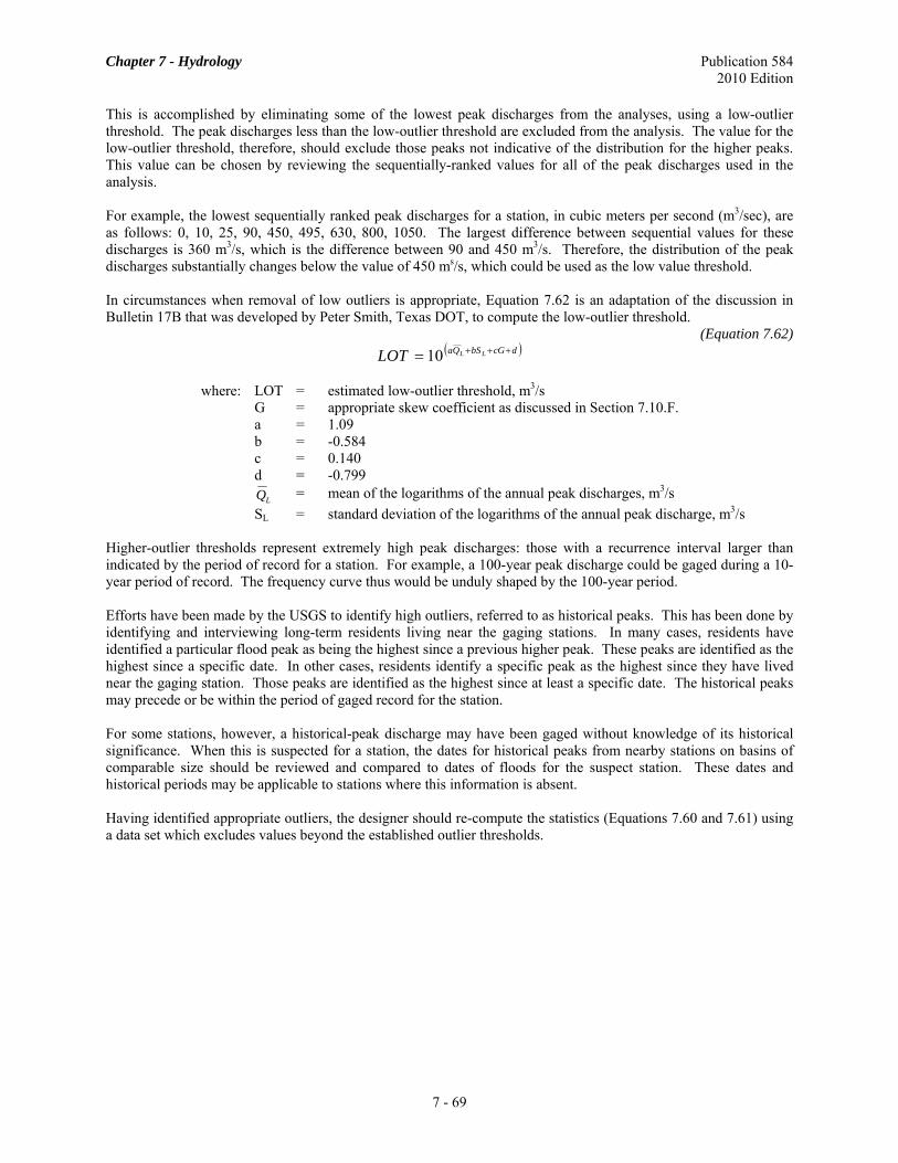
Chapter 7 - Hydrology Publication 584 2010 Edition
This is accomplished by eliminating some of the lowest peak discharges from the analyses, using a low-outlier threshold. The peak discharges less than the low-outlier threshold are excluded from the analysis. The value for the low-outlier threshold, therefore, should exclude those peaks not indicative of the distribution for the higher peaks. This value can be chosen by reviewing the sequentially-ranked values for all of the peak discharges used in the analysis. For example, the lowest sequentially ranked peak discharges for a station, in cubic meters per second (m3/sec), are as follows: 0, 10, 25, 90, 450, 495, 630, 800, 1050. The largest difference between sequential values for these discharges is 360 m3/s, which is the difference between 90 and 450 m3/s. Therefore, the distribution of the peak discharges substantially changes below the value of 450 ms/s, which could be used as the low value threshold. In circumstances when removal of low outliers is appropriate, Equation 7.62 is an adaptation of the discussion in Bulletin 17B that was developed by Peter Smith, Texas DOT, to compute the low-outlier threshold.
(Equation 7.62) ( )dcGbSQa LLLOT +++= 10
where: LOT = estimated low-outlier threshold, m3/s
G = appropriate skew coefficient as discussed in Section 7.10.F. a = 1.09 b = -0.584 c = 0.140 d = -0.799
LQ = mean of the logarithms of the annual peak discharges, m3/s SL = standard deviation of the logarithms of the annual peak discharge, m3/s
Higher-outlier thresholds represent extremely high peak discharges: those with a recurrence interval larger than indicated by the period of record for a station. For example, a 100-year peak discharge could be gaged during a 10-year period of record. The frequency curve thus would be unduly shaped by the 100-year period. Efforts have been made by the USGS to identify high outliers, referred to as historical peaks. This has been done by identifying and interviewing long-term residents living near the gaging stations. In many cases, residents have identified a particular flood peak as being the highest since a previous higher peak. These peaks are identified as the highest since a specific date. In other cases, residents identify a specific peak as the highest since they have lived near the gaging station. Those peaks are identified as the highest since at least a specific date. The historical peaks may precede or be within the period of gaged record for the station. For some stations, however, a historical-peak discharge may have been gaged without knowledge of its historical significance. When this is suspected for a station, the dates for historical peaks from nearby stations on basins of comparable size should be reviewed and compared to dates of floods for the suspect station. These dates and historical periods may be applicable to stations where this information is absent. Having identified appropriate outliers, the designer should re-compute the statistics (Equations 7.60 and 7.61) using a data set which excludes values beyond the established outlier thresholds.
7 - 69

Chapter 7 - Hydrology Publication 584 2010 Edition
7 - 70
Figure 7.11 Pennsylvania Generalized Skew Coefficients of Logarithms of Annual Maximum Streamflow (G)

Chapter 7 - Hydrology Publication 584 2010 Edition
7.11 CHAPTER 7 NOMENCLATURE
Symbol Definition Units
A Drainage area ha or ac A Channel cross-sectional area in Manning's Equation m2 of ft2 An Nth sub-area size ha or ac Ag Area of gaged basin ha or ac α 1.0 (metric), 3.28 (U.S. Customary) m/s or ft/s C Weighted runoff coefficient dimensionless c Wave celerity for use in Muskingum-Cunge Method m/s or ft/s Cf Runoff coefficient adjustment factor due to return interval dimensionless Cn Runoff coefficient for nth sub-area dimensionless C0, C1, C2 Coefficients for Unit Peak Discharge Equation dimensionless C1, C2, C3 Coefficients for Muskingum and Muskingum-Cunge Routing dimensionless d Duration of unit excess rainfall hr F Pond adjustment factor dimensionless G Skew coefficient for Log Pearson Type III curve fit dimensionless GS Coefficient of skew of log values, station skew dimensionless g Gravitational acceleration m/s2 or ft/s2 I Average rainfall intensity in the Rational Method Equation mm/hr or in/hr I Inflow to reach in the Muskingum Method m3/s or cfs Ia Initial abstraction mm or in It Inflow at time step number t for Hydrograph Routing m3/s or cfs It+1 Inflow at time step number t + 1 for Hydrograph Routing m3/s or cfs i Rainfall intensity in the Overland Flow Segmental Method mm/hr or in/hr K A frequency factor for Log Pearson Type III Analysis dimensionless K Coefficient for use in Sheet Flow Kinematic Wave Equation 6.92 Metric/0.933 US K Coefficient for use in the Rational Method Equation 360 Metric/1 US K Coefficient for use in the Triangular Hydrograph Method 0.208 Metric/484 US K Coefficient for Overland Flow Equation 2949 Metric/1900 US K Proportionality constant representing the time of travel of a
flood wave through the reach in the Muskingum method hr k Intercept coefficient for Shallow Concentrated Flow Equation dimensionless L Longest hydraulic length m or ft Ln Length of nth reach along flow path m or ft LOT Estimated low-outlier threshold for use in Bulletin 17B
Statistical Frequency Analysis m3/s μ Hydraulic diffusivity for use in Muskingum-Cunge Method m2/s or ft2/s N Number of observations dimensionless n Manning's n-value dimensionless O Outflow from reach in the Muskingum Method m3/s or cfs Ot Outflow at time step number t for Hydrograph Routing m3/s or cfs Ot+1 Outflow at time step number t + 1 for Hydrograph Routing m3/s or cfs P Accumulated rainfall (potential maximum runoff) for NRCS
Rainfall-Runoff Equation mm or in Q Discharge m3/s or cfs Q Maximum rate of runoff in the Rational Method Equation m3/s or cfs Q Flood magnitude m3/s or cfs
LQ Mean of the logarithms of the annual peak discharges in Log Pearson Type III Analysis m3/s or cfs
Qg WRC peak discharge at gage m3/s or cfs qx Lateral inflow or outflow in Muskingum-Cunge Method m2/s or ft2/s q Depth of storm runoff during time interval for Hydrograph
Methods mm or in qp Peak rate of discharge m3/s or cfs qu Unit peak discharge m3/s/km2/mm or cfs/mi2/in
7 - 71

Chapter 7 - Hydrology Publication 584 2010 Edition
R Runoff volume for NRCS Graphical Peak Discharge Method mm or in R Hydraulic radius in Manning's Equation m or ft RCN or CN Runoff Curve Number dimensionless S Average slope of the watershed in percent % S Potential max retention for NRCS Rainfall-Runoff Equation mm or in S Total Storage in the Muskingum Method m3 or ft3 Sf Friction slope m/m or ft/ft SL Standard deviation of logarithms of annual peak discharge m3/s or cfs So Channel bed slope m/m or ft/ft Sp Channel or flow slope in percent % Sr Volume of runoff completely retained for Storage-Indication
Method m3 or ft3 St Storage in the reservoir at time step number t for Hydrograph
Routing m3 or ft3 St+1 Storage in the reservoir at time step number t + 1 for
Hydrograph Routing m3 or ft3 s Surface slope of the flow path m/m or ft/ft T Total time along flow path in Time of Concentration
Calculation min Tlag SCS Lag time hr Tp Time to peak runoff in Hydrograph Methods hr t Time general Tc or tc Time of concentration hr tn Travel time over nth reach min tt Sheet flow travel time min V Velocity m/s or ft/s vn Estimated flow velocity for nth reach m/s or ft/s x Distance general X Backwater storage effects weighting factor in the
Muskingum method dimensionless X Logarithm of the annual peak discharge in Log Pearson
Type III Analysis m3/s or cfs Δ T Time increment general Σ It Sum of inflow hydrograph ordinates for Storage-Indication
Method m3 or ft3 ΣOt Sum of outflow hydrograph ordinates for Storage-Indication
Method m3 or ft3 7.12 REFERENCES AASHTO (2003). Highway Drainage Guidelines, Washington, DC: American Association of State Highway and Transportation Officials. AASHTO (2005). Model Drainage Manual, Washington, DC: American Association of State Highways and Transportation Officials. American Society of Civil Engineers (1949). Hydrology Handbook, Manuals of Engineering Practice, No. 28, prepared by the Hydrology Committee of the Hydraulics Division. Anderson, D. G. (1970). "Effects of Urban Development on Floods in Northern Virginia," U.S. Geological Survey Water Supply Paper 2001 C, Washington, DC: U.S. Government Printing Office. Arcement, G.J. Jr. and Schneider, V.R. (1989). Guide for Selecting Manning's Roughness Coefficients for Natural Channels and Flood Plains. U.S. Geological Survey Water-supply Paper 2339. Washington, DC: U.S. Government Printing Office.
7 - 72
Aron, G., and Kibler, D. F. (1981). Procedure PSU IV for Estimating Design Flood Peaks on Ungaged Pennsylvania Watersheds. University Park, PA: The Pennsylvania State University.

Chapter 7 - Hydrology Publication 584 2010 Edition
7 - 73
Baker, V. R., et al. (1979, December). "Long Term Flood Frequency Analysis Using Geological Data." Proceeding of the Canberra Symposium, IAHS AISH Publication No. 128. Baker, V. R. (1983). Paleoflood Hydrologic Techniques for the Extension of Streamflow Records. Transportation Research Board Record No. 922. Barnes, H. H., Jr. (1967). Roughness Characteristics of Natural Channels. U.S. Geological Survey Water Supply Paper 1849. Washington, DC: U.S. Government Printing Office. Benson, M. A. (1962). Evolution of Methods for Evaluating the Occurrence of Floods. U.S. Geological Survey Water Supply Page, 1580 A. Benson, M. A. (1964). Factors Affecting the Occurrence of Floods in the Southwest. U.S. Geological Survey Water Supply Paper 1580 D. Washington, DC: U.S. Government Printing Office. Benson, M. A., and Dalrymple, T. (1968). "General Field and Office Procedures for Indirect Discharge Measurement." U.S. Geological Survey, Techniques of Water Resources Investigations, Book 3, Chapter A1. Washington, DC: U.S. Government Printing Office. Bodhaine, G. L. (1968). "Measurement of Peak Discharge at Culverts by Indirect Methods," U.S. Geological Survey, Techniques of Water Supply Resources Investigations, Book 3, Chapter A3. Washington, DC: U.S. Government Printing Office. Bruce, S. A., et al. (1988, December). Flood Flow Characteristics of Wyoming Streams A Complication of Previous Investigations. Joint USGS and Wyoming Highway Department Report. Buchanan, T. J., and Somers, W. P. (1968). "Stage Measurements of Gaging Stations," U.S. Geological Survey, Techniques of Water Resources Investigations, Book 3, Chapter A7. Washington, DC: U.S. Government Print Office. Buchanan, T. J., and Somers, W. P. (1969). "Discharge Measurements at Gaging Stations," U.S. Geological Survey, Techniques of Water Resources Investigations, Book 3, Chapter AB. Washington, DC: U.S. Government Printing Office. Buchberger, S. G. (1981). Flood Frequency Analysis for Regulated Rivers. Transportation Research Board Record No. 832. Carter, R. W. (1961). Magnitude and Frequency of Floods in Suburban Areas. U.S. Geological Survey Professional Paper 424 B. Washington, DC: U.S. Government Printing Office. Carter, R. W., and Davidian, J. (1965). "Discharge Ratings at Gaging Station," U.S. Geological Survey, Surface Water Techniques, Book 1, Chapter 12. Washington, DC: U.S. Government Printing Office. Carter, R. W., and Davidian, J. (1968). "A General Procedure for Gaging Streams," U.S. Geological Survey, Techniques of Water Resources Investigations, Book 3, Chapter A6. Washington, DC: U.S. Government Printing Office. Chow, V. T. (1964). Handbook of Applied Hydrology. McGraw-Hill Book Company, New York. Chow, V. T. (1970). Open Channel Hydraulics. McGraw-Hill Book Company, New York. Chow, V. T., D. Maidment, and L. Mays (1988). Applied Hydrology. McGraw-Hill Book Company, New York. Craig, G., and Rankl, J. (1978). Analysis of Runoff from Small Drainage Basins in Wyoming. USGS Water Supply Paper 2056.

Chapter 7 - Hydrology Publication 584 2010 Edition
7 - 74
Cunge, J. A. (1969). "On the Subject of a Flood Propagation Computation Method (Muskingum Method)," Journal of Hydraulic Research, Vol 7, No. 2 pp 205-230. Dalrymple, T. (1960). Flood Frequency Analysis. U.S. Geological Survey Water Supply Paper 1543 A. Washington, DC: U.S. Government Printing Office. Dalrymple, T., and Benson, M. A. (1967). "Measurement of Peak Discharge by the Slope Area Method," U.S. Geological Survey, Techniques of Water Resources Investigations, Book 3, Chapter A2. Washington, DC: U.S. Government Printing Office. DeBarry, P.A. (2004). Watersheds: Processes Assessment and Management. Hoboken, NJ. John Wiley and Sons. Federal Aviation Agency. (1970). Airport Drainage. Department of Transportation, Advisory Circular, A1C 150 5320 5B. Washington, DC: U.S. Government Printing Office. Federal Highway Administration. (1980, March). Hydraulic Design of Bridges with Risk Analysis, FHWA-TS-80-226, 142p, National Technical Information Service PB81-104259. Federal Highway Administration. (1980, July). The Design of Encroachments on Flood Plains Using Risk Analysis. Hydraulic Engineering Circular No. 17. Federal Highway Administration. (1984, March). Drainage of Highway Pavements. Hydraulic Engineering Circular No. 12. Federal Highway Administration. (1984, October). Hydrology. Hydraulic Engineering Circular No. 19. Federal Highway Administration. (2002). Highway Hydrology. Hydraulic Design Series No.2, Second Edition. Fletcher, J. E., Huber, A. L., Haws, F. W., and Clyde, C. G. (1977). Runoff Estimates for Small Rural Watersheds and Development of a Sound Design Method. Research Report Prepared for the Federal Highway Administration by Utah State University. Fletcher, J. E., and Reynolds, G. W. (1972). Snowmelt Peak Flows and Antecedent Precipitation from Watersheds in Transition. American Water Resources Assoc. and Colorado State University. Fricke, T. J., Kennedy, M. R., and Wellington, N. B. (1983). "The Use of Rainfall Correlation in Determining Design Storms for Waterways on a Long Railway Line." Proceedings of the Hydrology and Water Resources Symposium, Hobart, Australia, November 8-10. Harley, B. M. (1978). Research on the Effects of Urbanization and Small Stream Flow Quantity. Report No. FHWA RD 78 88. Prepared for the Federal Highway Administration. Hedman, E. R., and Osterkamp, W. K. (1982). Streamflow Characteristics Related to Channel Geometry of Streams in Western United States. U.S. Geological Water Supply Paper 2193. Henderson, F.M. (1966). Open Channel Flow, MacMillan Publishing Co., New York, pp 265-267. Hiemstra, L. A. V. (1969). Joint Probabilities in the Rainfall - Runoff Relation. Transportation Research Board Record No. 261. Hiemstra, L. A. V., and Reich, B. M. (1967). Engineering Judgment and Small Area Flood Peak. Colorado State University Hydrology Paper No. 19, Ft. Collins, CO. Horner, W. E. (1910). "Modern Procedure in District Sewer Design," Engineering News, Vol. 64, p. 326. Horner, W. W., and Flynt, F. L. (1936). "Relation Between Rainfall and Runoff from Small Urban Areas," Trans. ASCE, Vol. 101.

Chapter 7 - Hydrology Publication 584 2010 Edition
7 - 75
Jarrett, R. (1986). Mixed Population Flood Frequency Analysis in Colorado. Transportation Research Board Record No. 1073. Jens, S. W. (1979). Design of Urban Highway Drainage, the State-of-the-Art. Prepared for the Federal Highway Administration. Jens, S. W., and McPherson, M. B. (1942). "Hydrology of Urban Areas," in Handbook of Applied Hydrology, Section 20. New York, NY: McGraw Hill Book Co., Inc. Leopold, L. B. (1968). Hydrology for Urban Land Planning - A Guidebook on the Hydrologic Effects of Urban Land Use. U.S. Geological Survey Circular 554. Washington, DC: U.S. Geological Survey. Linsley, R. K., Jr., Kohler, M. A., and Paulhus, J. L. H. (1975). Hydrology for Engineers, 2nd edition. McGraw Hill Book Company. Matthai, H. F. (1968). "Measurement of Peak Discharge at Width Contractions by Indirect Methods," U.S. Geological Survey, Techniques of Water Resources Investigations, Book 3, Chapter A5. Washington, DC: U.S. Government Printing Office. McCain, J. F., and Jarrett, R. D. (1976). Manual for Estimating Flood Characteristics of Natural Flow Streams in Colorado. USGS and Colorado Water Conservation Board. McCuen, R. H., and Miller, N. (1983). Conceptual and Empirical Comparison of Methods for Predicting Peak Runoff Rates. Transportation Research Board Record No. 922. Meinzer, O. E., ed. (1942). Hydrology. New York, NY: McGraw Hill Book Company, Inc. Miller, W. A., and Cunge, J. A. 1975. “Simplified Equations of Unsteady Flow,” Unsteady Flow in Open Channels, Vol I, K. Mahmood and V. Yevjevich, ed., pp 183-249. Mitci, C. (1974, January). "Determine Runoff by Simple Way," Water and Wastes Engineering, Vol. II, No. 1. National Resource Conservation Service (1985, March). National Engineering Handbook, Section 4, "Hydrology." Washington, DC: U.S. Government Printing Office. National Resource Conservation Service (1986, June). Urban Hydrology for Small Watersheds, 2nd ed. Technical Release No. 55. National Water Council, Department of Environment. (1981, September). Design and Analysis of Urban Storm Drainage - The Wallingford Procedure. Standing Technical Committee Reports, Volume 1 to 5. London, Great Britain. Newton, D. W., and Herrin, J. C. (1982). Assessment of Commonly Used Flood Frequency Methods. Transportation Research Board Record No. 896. Lowham, H. W. (1976). Techniques for Estimating Flow Characteristics of Wyoming Streams. U.S. Geological Survey Water Resources Investigations 76 112. Ragan, R. M. (1971, December). A Nomograph Based on Kinematic Wave Theory for Determining Time of Concentration for Overland Flow. Civil Engineering Research Report No. 44. College Park, MD: University of Maryland. Reich, B., and Aron, G. (1976, October). "Magnitude and Frequency of Flood," CRC Critical Reviews in Environmental Control, Vol. 6, Number 4, pp. 297 348. Reich, B. M., and Jackson, D. R. (1971). Flood Prediction Methods for Pennsylvania Highway Crossings. Research Report prepared by the Pennsylvania State University for the Pennsylvania Department of Transportation.

Chapter 7 - Hydrology Publication 584 2010 Edition
7 - 76
Rhodes, D. D., and William, G. (1979). Adjustments of the Fluvial System. Reference Section on Slack Water Deposits: A Geomorphic Technique for the Interpretation of Fluvial Paleohydrology by Peter C. Patton, Victor R. Baker, and R. Craig Kochel. Iowa: Kendall Hunt Publishing Co. Ribeny, F. M. J. (1971). "On the Chance of Culvert Washouts on a Long Railway Line." Hydrology Papers, Institution of Engineers, Australia. Riggs, H. C. (1968). "Frequency Curves," U.S. Geological Survey, Techniques of Water Resources Investigations, Book 4, Chapter A2. Washington, DC: U.S. Government Printing Office. Sanders, T. G. (1980, January). Hydrology for Transportation Engineers. Prepared by Colorado State University for the Federal Highway Administration. Sauer, V. B., Thomas, W. O., Jr., Stricker, V. A., and Wilson, K. V. (1983). Flood Characteristics of Urban Watersheds in the United States. Prepared in cooperation with the Federal Highway Administration, U.S. Geological Survey Water Supply Paper 2207. Schaake, J. C., Jr., Geyer, J. C., and Knapp, J. W. (1967). "Experimental Examination of the Rational Method," Proc. ASCE, Hydraulics Division Journal HY6 Paper 5607. Sherman, L. K. (1932). "Stream Flow from Rainfall by the Unit Graph Method," Eng. News Record, Vol. 108. Snyder, F. F. (1938). "Synthetic Unit graphs," Trans. Am. Geophys. Union, Vol. 19. Stockton, C. W., and Boggess, W. R. (1983). Tree Ring Data: Valuable Tool for Reconstructing Annual and Seasonal Streamflow and Determining Long Term Trends. Transportation Research Board Record No. 922. Stuckey, Marla H., and Reed, Lloyd A., 2000, Techniques for Estimating Magnitude and Frequency of Peak Flows for Pennsylvania Streams, U.S. Geologic Survey, Water-Resources Investigations Report 00-4189. Subcommittee on Hydrology, Inter Agency Committee on Water Resources (1966). "Methods of Flow Frequency Analysis," Notes on Hydrologic Activities, Bulletin No. 13. Washington, DC: U.S. Government Printing Office. Thomas, D. A., and Benson, M. A. (1970). Generalization of Stream Flow Characteristics from Drainage Basin Characteristics. U.S. Geological Survey Water Supply Paper No. 1975. Tice, R. H. (1958). Delaware River Basin Flood Frequency. U.S. Geological Survey open file report, Trenton, N.J. U.S. Bureau of Public Roads (1965). Design of Roadside Drainage Channels. Hydraulic Design Series No. 4. U.S. Department of the Interior, Bureau of Reclamation (1973). Design of Small Dams, 2nd ed. U.S. Federal Council for Science and Technology, Ad Hoc Panel on Hydrology. (1962, June). Scientific Hydrology. Washington, DC. U.S. Geological Survey (1998). Users Manual for Program PEAKFQ, Annual Flood Frequency Analysis Using Bulletin 17B Guidelines. U.S. Geological Survey (1998). Water-Quality Conditions During Low Flow in the Lower Youghiogheny River Basin, Pennsylvania, October 5-7, 1998. Water-Resources Investigations Report 01-4189. U.S. Geological Survey (2002). The National Flood Frequency Program, Version 3, Water-Resources Investigations Report 02-4168. U.S. Geological Survey (2008a). Regression Equations for Estimating Flood Flows at Selected Recurrence Intervals for Ungaged Streams in Pennsylvania, Scientific Investigations Report 2008-5102, USGS, Reston, VA 2008.

Chapter 7 - Hydrology Publication 584 2010 Edition
7 - 77
U.S. Geological Survey (2008b), Ries III, Kernell G., Guthrie, John G., Rea, Alan H., Steeves, Peter A., and Stewart, David W., StreamStats: A Water Resources Web Application, USGS Fact Sheet FS 2008-3067, USGS, Reston, VA 2008. U.S. Water Resources Council (1982, March). Guidelines for Determining Flood Flow Frequency. Bulletin 17B. Wacker, A. M. (1974, June). Highway Impact on a Mountain Stream. M.S. Thesis, Colorado State University. Wahl, K. L. (1983). Determining Streamflow Characteristics Based on Channel Cross Section Properties. Transportation Research Board Record No. No. 922. Wilson, K. V. (1967). A Preliminary Study of the Effect of Urbanization on Floods in Jackson, Mississippi. U.S. Geological Survey Professional Paper 575 D. Washington, DC: U.S. Government Printing Office. Wisler, C. O., and Brater, E. F. (1959). Hydrology, 2nd ed. New York, NY: John Wiley and Sons, Inc.

Chapter 7 - Hydrology Publication 584 2010 Edition
7 - 78
BLANK PAGE