hydrology, hydrodynamics and juvenile salmon...

Hydrology, Hydrodynamics and Juvenile Salmon entrainment rate estimates:implications for a proposed notch

in the Fremont Weir

Aaron Blake, Paul Stumpner, and Jon Burau USGS California Water Science Center

Delta Science Panel Review Dry Run - July 31, 2017

Jon Burau

Introductory Remarks

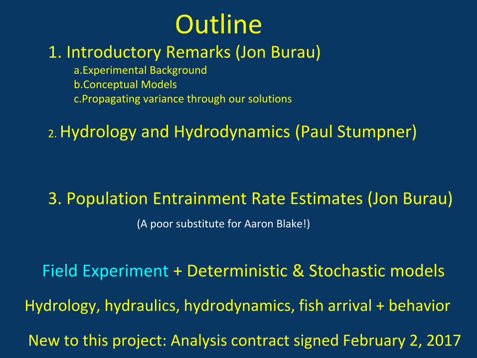
Outline1. Introductory Remarks (Jon Burau)

a.Experimental Backgroundb.Conceptual Modelsc.Propagating variance through our solutions

2. Hydrology and Hydrodynamics (Paul Stumpner)

3. Population Entrainment Rate Estimates (Jon Burau)(A poor substitute for Aaron Blake!)

Field Experiment + Deterministic & Stochastic models

Hydrology, hydraulics, hydrodynamics, fish arrival + behavior

New to this project: Analysis contract signed February 2, 2017

Began 2D telemetry studies in 20064 Years of studies at Georgiana Slough

~ 11K tagged fish

The tools developed in these studies were applied to Fremont Weir Project

Funding provided by DWRProject managers: Jacob McQuirk and Ryan Reeves

DWR. (2012). 2011 Georgiana Slough Non-Physical Barrier Performance Evaluation Project Report. Bay-Delta Office, Sacramento, California.http://bayDeltaoffice.water.ca.gov/sdb/GS/docs/GSNPB_2011_Final_Report+Append_090512.pdf

DWR (2015). 2012 Georgiana Slough Non-Physical Barrier Performance Evaluation Project Report. Bay-Delta Office, Sacramento, California.http://bayDeltaoffice.water.ca.gov/sdb/GS/docs/Final%20GSNPB%202012%20Report_Review%20Certified.pdf

DWR (2016). 2014 Georgiana Slough Floating Fish Guidance Structure Performance Evaluation Project Report. Bay-Delta Office, Sacramento, California.http://bayDeltaoffice.water.ca.gov/sdb/GS/docs/Final%20Report%20October%202016%20Edition%20103116-signed.pdf

Working on contract with DWR to in peer reviewed Literature

http://baydeltaoffice.water.ca.gov/sdb/GS/docs/Final%20Report%20October%202016%20Edition%20103116-signed.pdf

2D tracking of tagged fish in the Sac River adjacent to the fremont Weir 2015

(stage too low - not used in the present analysis) Cooperators (COE, USBR, DWR)

Funding USBR

Ref: Anna Steele - Supplemental Docs

USGS Tracking AlgorithmSpatial Aggregation Software

Spatial Aggregation from 2015 data

Steele used Kernel densities forSpatial aggregation = residence time

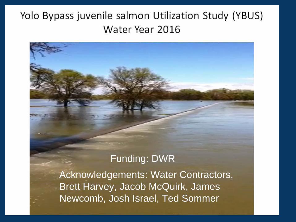
Acknowledgements: Water Contractors, Brett Harvey, Jacob McQuirk, James Newcomb, Josh Israel, Ted Sommer

Funding: DWR

Our Field Teams are awesome!Chris Vallee and Co.:Deployment and recovery of telemetry gear

Marty (Theresa) Liedke and Co.: Fish handling/release

In 2016: Smolts were huge.. ~165mm

Fry (~ 35-55mm) are likely to get the biggest benefit from Yolo Bypass

Conceptual Models

(1)Critical Streakline

(2) Secondary Circulation

Critical Streakline

Entrainment rate = f(co-occurrence of Streakline position

and fish distribution)

Fish don’t “go the flow” (discharge)!

In most cases fish “go with” their local velocity (advection >> fish swimming performance)

Still….behavior is observable in our data sets

Perry, Russell W.; Buchanan, Rebecca A.; Brandes, Patricia L.; Burau, Jon R.; & Israel, Joshua A.(2016). Anadromous Salmonids in the Delta: New Science 2006–2016. San Francisco Estuary and Watershed Science, 14(2). jmie_sfews_31668. Retrieved from: http://escholarship.org/uc/item/27f0s5kh

PERRY R.W., J. G. ROMINE, N. S. ADAMS , A. R. BLAKE , J. R. BURAU , S. V. JOHNSTON and T. L. LIEDTKE (2012) USING A NON-PHYSICAL BEHAVIOURAL BARRIER TO ALTER MIGRATION ROUTING OF JUVENILE CHINOOK SALMON IN THE SACRAMENTO–SAN JOAQUIN RIVER DELTA RIVER RESEARCH AND APPLICATIONS River Res. Applic. (2012) DOI: 10.1002/rra.2628

Needs behavior to work!

Spatial Aggregation from 2015 data

Entrainment depends on the covariance of:

(1) Backwater - affects stages, discharges and the details of the hydrodynamics near the notch, including the location of critical streakline and secondary circulation.

(2) Stage can change VERY rapidly (0.25 ft/hr ~ max 0.5 ft/hr), often when the endangered runs (episodic) are moving through the system

(3) Arrival time distribution - function of run, upper watershed hydrologic response.

(4) Individual fish behavior

Propagating Variance through our solutions

Variance in Backwater in Sacramento River(from Feather River and Sutter Bypass)

10-12,000 CFS

Sutter Bypass and Feather River are often flowing pretty good at the notch activation stages

Green Line = 2016 Index Velocity dataRed Line = Data from Regression (1989-2017)

90-th percentile lines

Notch in Play

Rating tighter

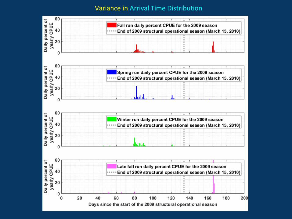
Variance in Arrival Time Distribution

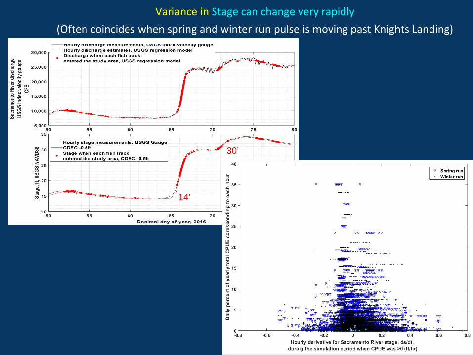
Variance in Stage can change very rapidly(Often coincides when spring and winter run pulse is moving past Knights Landing)

14’

30’

Variance in Individual Fish Behavior

All Tracks

Barrier OFF

Barrier ON

Questions?

The rest of our talks are about what we did, how we handled variance in our covariates, and what we learned.

Hydrology and Hydrodynamics on the Sacramento River near the Fremont

Weir: Implications for Juvenile Salmon Entrainment Estimates

Paul Stumpner, Aaron Blake, and Jon Burau USGS California Water Science Center

Delta Science Panel Review Dry Run - July 31, 2017

Paul Stumpner

PRESENTATION OUTLINE

1. Variance in the Stage-Discharge Relationship● Estimating the degree of backwater

2. Application of Conceptual Models used in our Analysis ● Secondary Circulation in Bends ● Critical Streakline; Entrainment Zone

3. Accounting for Variance in the Stage-Discharge Relationship● 3D Interpolant - to account for unmeasured conditions for

entrainment simulations● Estimate the variance in the location of the critical streakline

4. Summary and Key Findings

2016 YBUS STUDY AREA

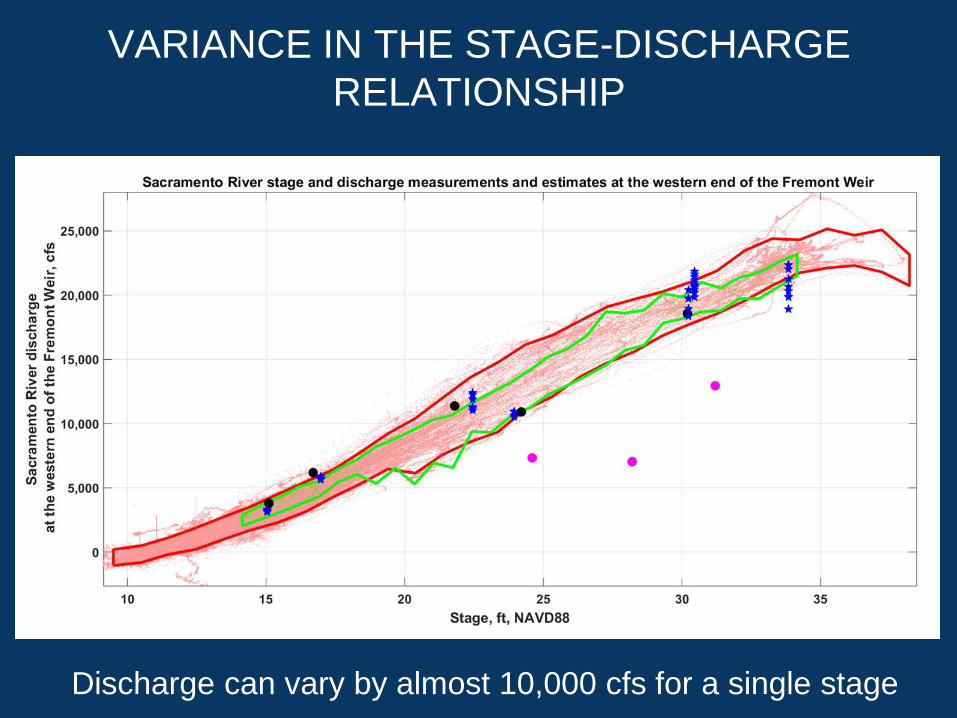
VARIANCE IN THE STAGE-DISCHARGE RELATIONSHIP

Discharge can vary by almost 10,000 cfs for a single stage

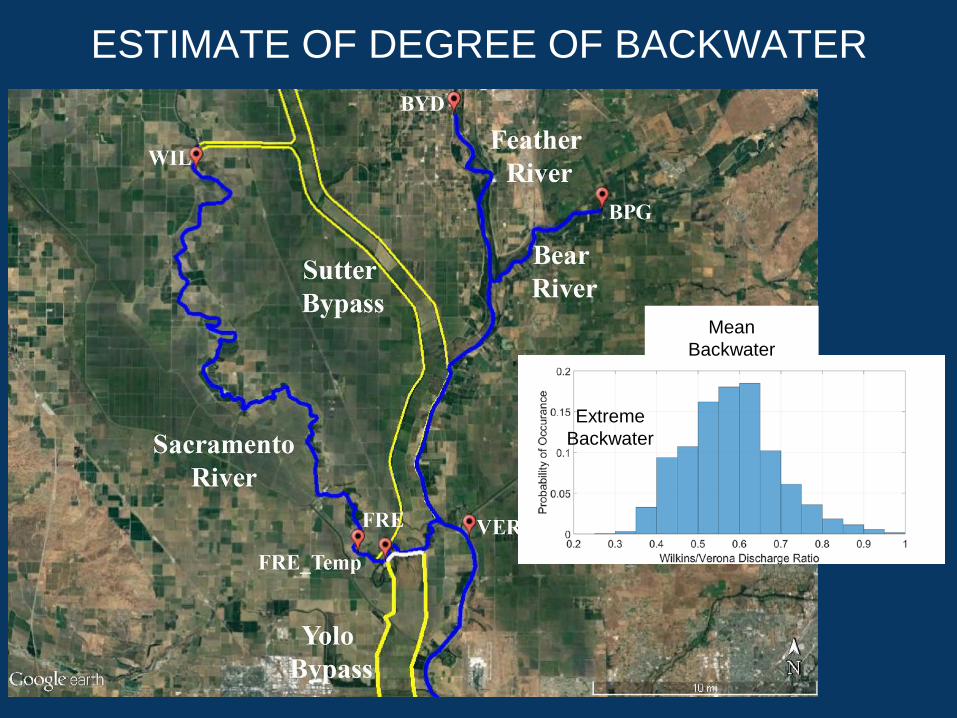
ESTIMATE OF DEGREE OF BACKWATER

Mean Backwater

Extreme Backwater

Conditions Measured

Stage NAVD88(ft)

Discharge(cfs)

15.1 8,790

16.7 11,200

21.8 16,380

24.2 15,920

24.6 12,340

28.2 12,030

30.2 23,590

31.2 17,950

BACKWATERED

CROSS-SECTION LOCATIONS OF VELOCITY TRANSECTS

Flow Direction

VELOCITY TRANSECTS TO DOCUMENT SECONDARY CIRCULATION

32.3’ - Height of Weir

29’ - Height where river overbanks

channel

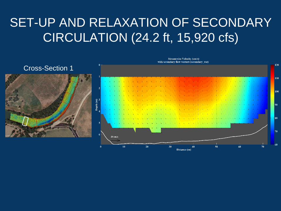
Cross-Section 1

SET-UP AND RELAXATION OF SECONDARY CIRCULATION (24.2 ft, 15,920 cfs)

Cross-Section 4


Cross-Section 7


HYDRAULIC ENTRAINMENT ZONE ESTIMATE USING THE CRITICAL STREAKLINE METHOD

ESTIMATING ENTRAINMENT BY COMPARING WATER AND FISH CDF FUNCTIONS

Integrate along the cross section

Estimated cross section PDFs Estimated cross section CDFs

Meters from right bank (diversion)

Not Entrained Entrained

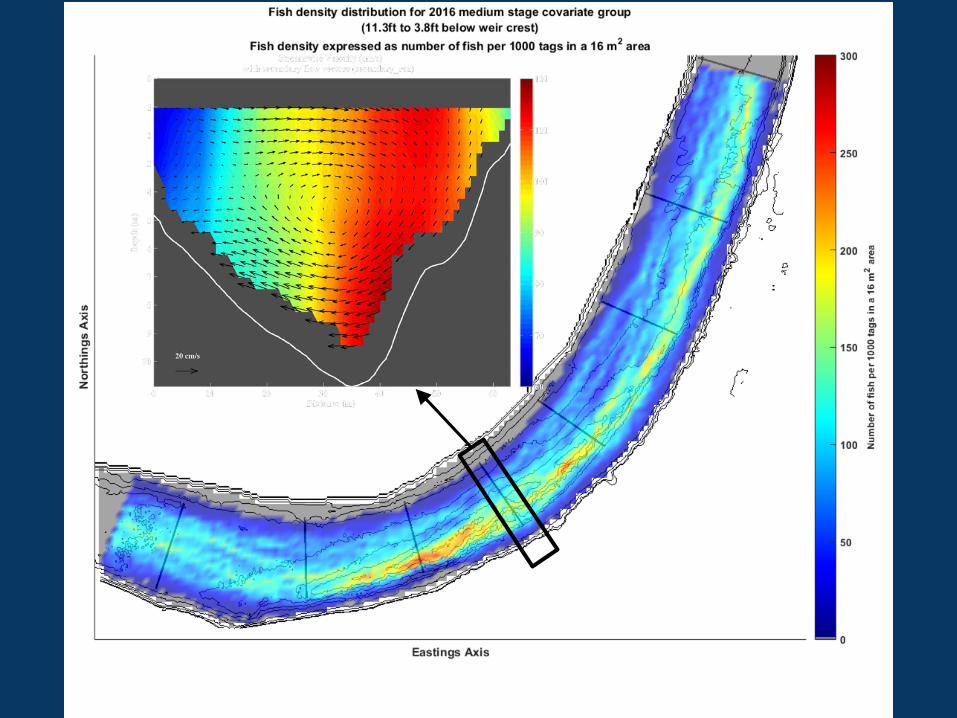
COMBINING FISH DENSITY AND FLOW DENSITY

Velocity: 24ft, 17,800 cfsFish: 21ft, 14,800 cfs

28.5ft, 22,400 cfsNotch: 8.7%, 1,547 cfs

Velocity: 24ft, 17,800 cfsFish : 21ft, 14,800 cfs

28.5ft, 22,400 cfsNotch : 8.7%, 1,547 cfs

COMBINING FISH DENSITY AND FLOW DENSITY

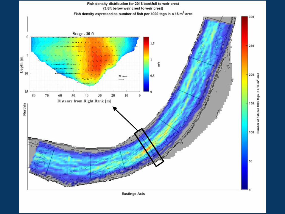
Fish Spatial Distribution High Stage 28.5 ft. - 32.3 ft.Shaded Grey - Wetted Area

More flow towards INSIDE of bend

More flow towards OUTSIDE of bend

IN ORDER TO MAKE ACCURATE HYDRAULIC ENTRAINMENT ZONE ESTIMATES

1. Account for limited range of measured conditions; 8 different conditions (5 during mean backwater, 3 during extreme backwater).● 5 Discharge CDFs are interpolated in the along stream

direction and with stage to generate a 3D interpolant● Best notch location varies as a function of stage and

discharge ratio

2. Estimate the variance in the location of the critical streakline due to variance in the stage-discharge relationship.

● Note that discharge can vary by ~ 10,000 cfs for a given stage

● We have two sets of similar stage conditions with different discharge

24.2 ft, 15,920 cfs and 24.6 ft, 12,340 cfs30.2 ft, 23,590 cfs and 31.2 ft, 17,950 cfs

● The maximum difference in the critical streakline between these two set of conditions is 5.4 m.

ESTIMATE OF VARIANCE IN THE LOCATION OF THE CRITICAL STREAKLINE

● Represent variance stochastically with a random effects model since we lack the data to explicitly define the variance for a set of conditions.

● Wilkins/Verona discharge ratio can be approximated by a normal distribution and largest difference is 5.4 m with a 0.305% chance of occurrence.

● We set the variance in critical streakline as a normal distribution with a mean of 0 and a standard deviation of 1.97 m that produces an difference of 5.4 m that occurs 0.305 % of the time

● Additional sources of error (bank estimate and velocity extrapolation) produce difference in the critical streakline < 1m.

● Since additional sources of error are smaller in magnitude than the magnitude of variance in the random effect model, we only use the random effect model


CONCLUSIONS

● Generally, Secondary circulation redistributes water mass and fish mass towards outside of the bend

● Fish entrainment likely will be maximal near the river bend

● Critical Streakline method has been a good predictor of fish entrainment at junctions in past studies, and will likely work well at this location

● Fish and water mass distribution can change after river overbanking and with stronger backwater conditions

● Variance in the stage-discharge relationship produces the greatest source of variance in the critical streakline and ultimately fish entrainment estimates

• Fish Data - Aaron Blake, Anna Steel, University of California, Davis / ERDC, US Army Corps of Engineers

• Cartoon (Conceptual) Design - Jon Burau

• Data Collection – USGS Field Crews: Chris Vallee, Jim DeRose, Trevor Violette, Matt Sholtis, Nick Swyers

• Funding - Department of Water Resources

• Other collaborators Army Corps of Engineers, USBR and UC Davis

AKNOWLEDGEMENTS

Questions?

Aaron Blake, Paul Stumpner, and Jon Burau, USGS California Water Science Center

USGS Entrainment Analysis

Review panel summary of USGS draft entrainment analysis, 9/7/17


USGS entrainment analysis: Purpose and scopeThe USGS Analysis was confined toevaluating alternatives on the western end of the Fremont Weir.

The only data we have (2016).


USGS entrainment analysis: Purpose and scope

Within this region our analysis was focused on answering the following questions:

1. To what extend does the location of each alternative within the study area affect the entrainment?

2. Which location(s) result in the highest entrainment for each alternative?

3. To what extend does outmigration timing and seasonal variance in hydrology affect the location that produces maximum entrainment for each alternative?

4. What general strategiesmight we use to increase entrainment through a notch in the Fremont Weir?


USGS entrainment analysis: 2016 fish track data collection● The study fish were 165 mm late fall run Chinook salmon smolts from the Coleman National Fish

Hatchery.

● Fish were tracked using VEMCO HRR receiversdeployed in the Sacramento River in the vicinity of the western end of the Fremont Weir.

VEMCO provided the USGS with time-synchronized detections and the USGS used the GenticFish algorithm to produce an independent set of tracks. The USGS tracks were used for the entrainment evaluation.

A small number of tracks were removed from the analysis pool due to poor tracking performance or predator-like movement patterns (swimming up stream).

The remaining 633 tracks were extrapolated and interpolated prior to the entrainment analysisusing an along-channel, cross-channel curve linear coordinate system.


USGS entrainment analysis: fish tracking array


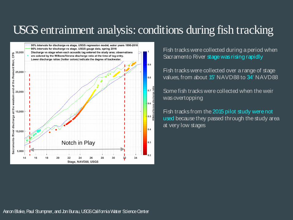
USGS entrainment analysis: conditions during fish trackingFish tracks were collected during a period when Sacramento River stage was rising rapidly

Fish tracks were collected over a range of stage values, from about 15’ NAVD88 to 34’ NAVD88

Some fish tracks were collected when the weir was overtopping

Fish tracks from the 2015 pilot study were not used because they passed through the study area at very low stages

Notch in Play


USGS entrainment analysis: why we chose a simulation approach

Evaluating the entrainment potential of an alternative at any location requires an analytical approach that accounts for the joint probability

distribution of (1) each run migrating through the study area under any pair of Sacramento River (2) stage and (3) discharge values.

Entrainment Potential = joint probability distribution of: (run timing, stage, discharge).


USGS entrainment analysis: Overview of simulation method

We used a Monte Carlo bootstrap simulation to evaluate entrainment for each alternative at 63 possible notch locations within the study area.

● We used historic Sacramento River stage and discharge, and Knights Landing screw trap data from water years 1996-2010 to provide the empirical joint probability of run timing as a function of discharge and stage.

● We used the fish tracks and hydrodynamic data collected during the 2016 study to estimate entrainmentgiven the Sacramento River stage and discharge conditions that occurred at each timestep.


USGS entrainment analysis: Overview of simulation methodThis process was repeated at every time step, for every run, for each scenario, at each notch evaluation location

This drawing is only a conceptual cartoon!


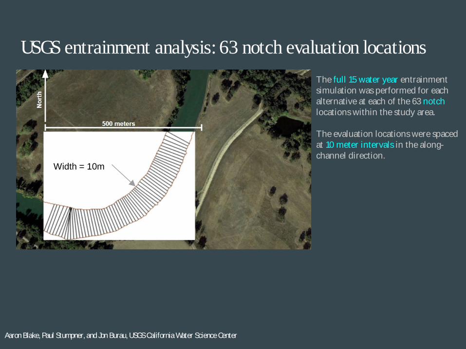
USGS entrainment analysis: 63 notch evaluation locationsThe full 15 water year entrainment simulation was performed for each alternative at each of the 63 notchlocations within the study area.

The evaluation locations were spaced at 10 meter intervals in the along-channel direction.

Width = 10m


USGS entrainment analysis: historic abundance data● We used Knights Landing catch data from water years 1996-2011 to estimate the historic abundance of:

○ Juvenile fall run Chinook salmon○ Juvenile spring run Chinook salmon○ Juvenile winter run Chinook salmon○ Juvenile late fall run Chinook salmon

● Catch data was expressed in terms of daily percent of yearly catch per unit effort - this means that each year was weighted equally within the simulation.

● The daily catch data was equally distributed between 4 hour time steps - this created a uniform probability with respect to catch as a function of hour within a day.

● The number of bootstrap samplesused at each timestep was determined by the normalized catch data for each run.

● We used bivariate weighted random sampling based on stage and discharge to draw the bootstrap sample from the pool of all 2016 fish tracks for each time step.

Variance in run timing = (# of bootstrap samples)Covariance in stage and discharge = (bivariate weighted random sampling)


USGS entrainment analysis: scenarios● Scenario 1: alternative 3 notch design, single notch alternative, flow ramps up at ~ 19ft, max notch flow

~6,100 cfs @ 31ft

● Scenario 2: alternative 4 notch design, single notch alternative, flow ramps up at ~ 19ft, max notch flow ~ 3,200 cfs @ 27ft

● Scenario 3: alternative 6 notch design, single notch alternative, flow ramps up at ~ 20 ft, max notch flow ~12,000 cfs @ 30 ft

● Scenario 4: analytical scenario based on the alternative 4 notch design but with the invert lowered 4 feet. Single notch alternative, flow ramps up at ~ 15ft, max notch flow ~ 3,200 cfs @ 23ft

● Scenario 5: alternative 5 notch design, multiple notch alternative, flow ramps up at ~ 16.3ft, complex combined rating curve, notch flow between ~3,000 cfs and ~3,500 cfs from 26.3ft to 32ft.

● Scenario 6: analytical scenario based on the alternative 5 notch design but with the invert lowered 1.6 feet. Multiple notch alternative, flow ramps up at ~ 15ft, complex combined rating curve, notch flow between ~3,000 cfs and ~3,500 cfs from 25ft to 32ft.


USGS entrainment analysis: adding analytical alternativesStage, discharge, and notch discharge ratio were highly correlated between all of the alternatives evaluated in the simulation.

The correlation between covariates made it hard to understand the mechanisms underlying notch performance because the effects of each covariate could not be evaluated independently.

We added two “analytical alternatives” to provide a means of evaluating the effects of discharge ratio and stage independently.

These analytical alternatives represented “deeper” (lower the invert) versions of Alternative 4 and Alternative 5 with their invert elevations lowered to begin taking water at 15’.


USGS entrainment analysis: scenario rating curves

Multi-gate

Single-gateAnalytical

Analytical


USGS entrainment analysis: summary of results Average percent of yearly population entrained (90% CI)

Run Scenario 1(alternative 3)Single Gate

Scenario 2(alternative 4)Single Gate

Scenario 3(alternative 6)Single Gate

Scenario 4(alternative 4

analytical)Single Gate

Scenario 5(alternative 5)

Multi Gate

Scenario 6(alternative 5

analytical)Multi Gate

Peak notch flow

6,100 cfs 3,200 cfs 12,000 cfs 3,200 cfs 3,400 cfs 3,400 cfs

Peak notch DR 0.26 0.17 0.57 0.23 0.17 0.19

Fall Run 12% (6%-21%) 9% (2%-21%) 28% (12%-43%) 15% (3%-28%) 6% (2%-12%) 7% (1%-15%)

Spring Run 9% (4%-15%) 7% (4%-14%) 22% (6%-42%) 16% (9%-20%) 5% (2%-11%) 6% (3%-13%)

Winter Run 5% (0%-12%) 4% (0%-11%) 11% (0%-38%) 9% (1%-20%) 2% (0%-10%) 3% (0%-11%)

Late Fall Run 9% (2%-17%) 7% (2%-15%) 23% (4%-42%) 15% (8%-23%) 5% (1%-11%) 6% (2%-12%)

Maximum entrainment

Location

38 38 30 38 15 15


USGS entrainment analysis: location and entrainment

Scour Hole Scour Hole


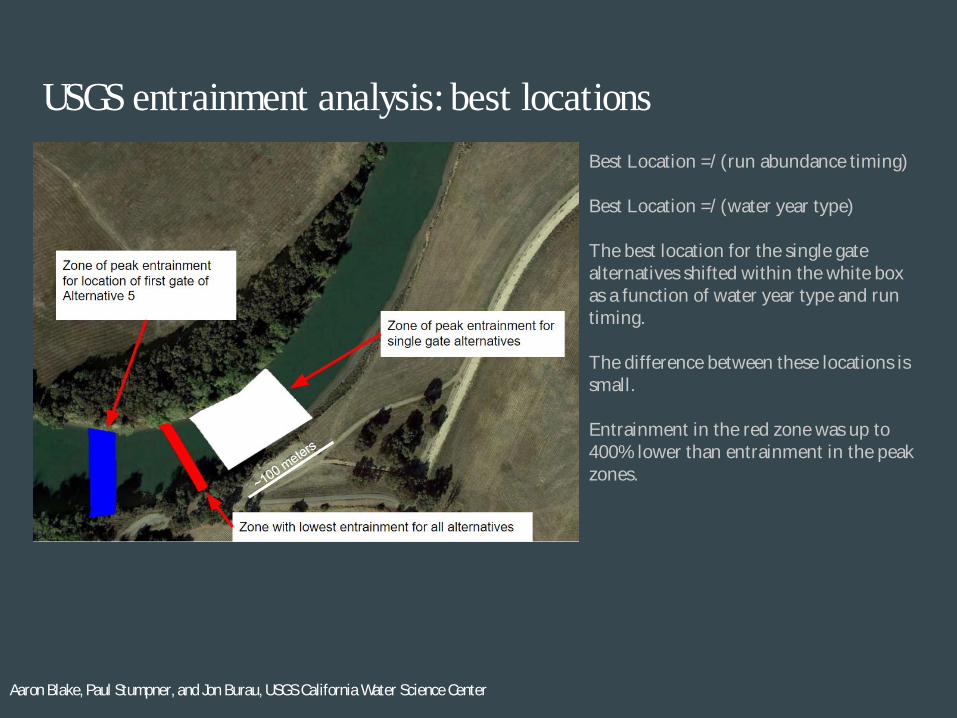
USGS entrainment analysis: best locationsBest Location =/ (run abundance timing)

Best Location =/ (water year type)

The best location for the single gate alternatives shifted within the white box as a function of water year type and run timing.

The difference between these locations is small.

Entrainment in the red zone was up to 400% lower than entrainment in the peak zones.


USGS entrainment analysis: the worst location

There is a scour hole in the river right bank of the Sacramento River in the region with lowest entrainment (red zone on prior slide).

Water velocities were very high near the bank at this location.

Scour Hole


USGS entrainment analysis: the worst location

Fish density was very low near the bank at scour hole

It is likely that fish were responding to turbulence and avoided the near-bank area near the scour hole.


USGS entrainment analysis: summary of key findings1. For each scenario notch location had a large impact on notch performance.

2. There was a ~100m long zone that resulted in near-maximum entrainment for all single notch alternativesadjacent to the western terminus of the Fremont Weir.

3. Maximum entrainment for multigate scenarios occurred when the first gate was located about 150 meters upstream of the single gate “peak zone”.

4. These locations were consistently the best across a diverse range of run abundance timing and seasonal hydrology.

5. Deepening (lowering invert) alternative 4 produced a significant increase in the number of spring run, winter run, and late fall run entrained under scenario 4.

6. Entrainment efficiency declined when the Sacramento River was above bankfull.(Centralization of downwelling zone)

7. Bathymetry upstream of a notch can strongly affect entrainment.


USGS entrainment analysis: primary sources of uncertainty

1. The use of large (~164mm fl) hatchery late fall run smoltsas surrogates for naturally migrating juvenile salmonids.

2. The limited range of conditions during experiment (Both backwater conditions and other covariates).

3. The limited range of backwater conditions represented within the water velocity measurements. (We tried to account for this stochastically).

4. The potential for notch modifications to alter the hydrodynamics in the study area (Primarily a concern for scenario 3).

5. The potential for upstream gate flows to alter fish tracks (multigate scenarios).


Questions?


~25% of spring run yearly CPUE was caught when Sacramento River stage was between 19’ and 22’


~25% of spring run and winter run yearly CPUE was caught when Sacramento River stage was between 19’ and 22’


USGS entrainment analysis: entrainment efficiency

Entrainment efficiency = fraction of fish entrained / fraction of water entrained

Entrainment efficiency > 1 ; more fish than water

Entrainment efficiency = 1 ; equal water and fish

Entrainment efficiency < 1 ; more water than fish


USGS entrainment analysis: entrainment efficiencyKey findings from entrainment efficiency analysis:

1. Single gate alternatives reached peak entrainment efficiency around 24’-25’, multi gate alternatives reached peak entrainment efficiency around 27’

1. Entrainment efficiency for all alternatives declined at bankfull (28.5’)

1. Entrainment efficiency for single gate alternatives declined below 1 for stages above bankfull, except for scenario 3 which maintained an efficiency of ~1 for stages above bankfull

1. Entrainment efficiency for multigate alternatives were higher than single gate alternatives (except scenario 3) for above bankfull conditions


USGS entrainment analysis: summary of key findings1. For each scenario notch location had a large impact on notch performance.

1. There was a ~100m long zone that resulted in near-maximum entrainment for all single notch alternatives adjacent to the western terminus of the Fremont Weir.

1. Maximum entrainment for multigate scenarios occurred when the first gate was located about 150 meters upstream of the single gate “peak zone”.

1. These locations were consistently the best across a diverse range of run abundance timing and seasonal hydrology.

1. Deepening alternative 4 produced a significant increase in the number of spring run, winter run, and late fall run entrained under scenario 4.

1. Entrainment efficiency declined when the Sacramento River was above bankfull.

1. Local bathymetry upstream of a notch could adversely affect entrainment.


USGS entrainment analysis: next steps

1. Possible final simulation runs to “tidy up” some details and respond to reviewer comments.

1. Possible addition of constant discharge ratio analytical alternatives to better understand peaks in entrainment efficiency.


USGS entrainment analysis: Entrainment Rate


Questions?


24.6 ft, 15,930 cfs 0.47 Wilkins/VeronaMean backwater condition

24.2 ft, 12,260 cfs0.37 Wilkins/VeronaBackwater condition

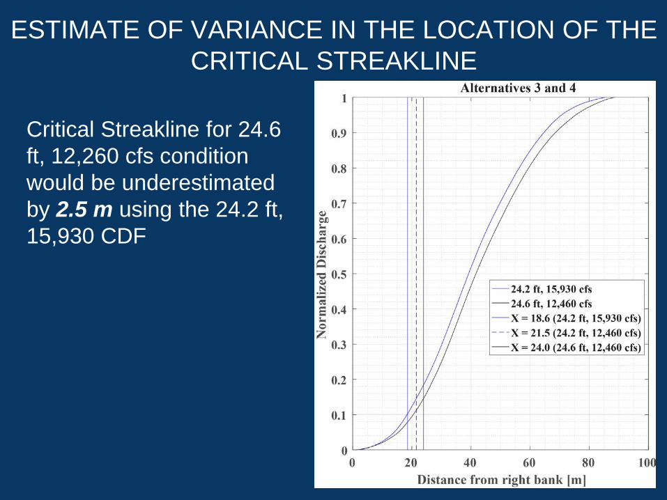
Critical Streakline for 24.6 ft, 12,260 cfs condition would be underestimated by 2.5 m using the 24.2 ft, 15,930 CDF


3D CDF INTERPOLANT MEAN BACKWATER CONDITION

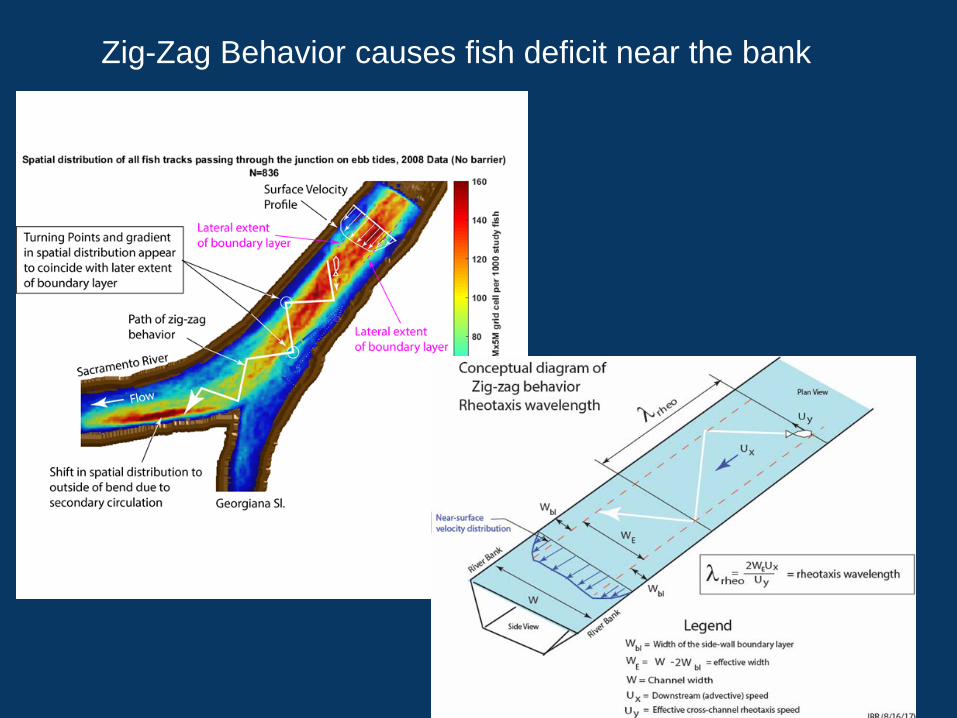
Zig-Zag Behavior causes fish deficit near the bank

JSAT Discussion

Smolts were huge.. ~165mm 2016 - Fry are likely to get the biggest benefit from Yolo BypassFry ~ 35-55mm

New tag 0.22g which will allow us to tag a fish down to 4.5 g >5% body burden.which gets us in the 55-100mm range, but.. we can select non-smolted fish (At least Parr).

Fry are 35-55mm fish and weigh 0.4-1.4 g.

hydrology, hydrodynamics and juvenile salmon...

Documents