Hydromulching in Tidally Influenced Wetlands:

Testing methods to alleviate seed wash-away and revegetate native plant communities

by

Allie A. Denzler

A Thesis

Submitted in partial fulfillment

of the requirements for the degree

Master of Environmental Studies

The Evergreen State College

May 2017

©2017 by Allie A. Denzler. All rights reserved.

This Thesis for the Master of Environmental Studies Degree

by

Allie A. Denzler

has been approved for

The Evergreen State College

by

________________________

Kevin Francis Ph. D.

Member of the Faculty

________________________

Date

ABSTRACT

Hydromulching in Tidally Influenced Wetlands:

Testing methods to alleviate seed wash-away and revegetate native plant communities

Allie A. Denzler

Estuaries are one of the most productive, and degraded, ecosystems on earth. Functioning

estuaries provide habitat for 75% of the U.S. commercial fish catch, yet large-scale

conversion of these wetlands to agricultural uses has resulted in estuarine habitat loss of

up to 60% in some areas. With the advent of the National Estuary Program in 1987, local

programs were developed to restore lost habitat functionality. Restored or created tidal

wetland projects often include a revegetation facet to kick-start productivity and habitat

development. Direct-seeding methods of revegetation have been the most cost-efficient,

however seed wash-away has been a problem in establishing planned native plant

communities in tidally influenced wetlands. This thesis tests a direct-seeding method

augmented by the addition of a layer of hydromulch (a water and wood mulch slurry) in a

set of recently created tidal channels on the Bayshore Preserve, in Shelton, Washington,

U.S.A. We compared first season recruitment densities of one native salt-tolerant forb

and four graminoid species under five different treatment conditions—broadcast seeded,

two seeded treatments augmented by burlap or hydromulch, and two controls. The forb

species, A. patula, was found to have statistically significant (p<.0007) higher stem

densities in treatments which implemented a burlap fabric and hydromulch layer over the

broadcast seed. The four graminoid species (C. lyngbyei, C. obnupta, E. palustris, & S.

americanus) did not germinate in this experiment. While seeding A. patula into created

tidal channels using this method shows promise, further research is needed to determine

if it is feasible for other species and whether survivability in subsequent seasons

compares with other wetland revegetation methods.

iv

Table of Contents

List of Figures…………………………………………………………………………….v

List of Tables ..................................................................................................................... v

Acknowledgements .......................................................................................................... vi

Introduction ....................................................................................................................... 1

Chapter 1: Bayshore Preserve Site History & Restoration Significance ..................... 5

1.1 Site use history................................................................................................................ 5

1.2 Capitol Land Trust Restoration Plan........................................................................... 7

1.3 Biodiversity of the Oakland Bay Area ............................................................................... 8

Chapter 2: Literature Review ........................................................................................ 11

2.1 Tidal Wetland Restoration ................................................................................................ 11

2.2 Tidal Marsh Revegetation Methods ................................................................................. 14

2.3 Hydromulching in Restoration Projects .......................................................................... 17

2.4 Species Selection ................................................................................................................. 19

2.5 Implications ........................................................................................................................ 22

Chapter 3: Methods and Materials ............................................................................... 24

3.1 Seed Preparation ................................................................................................................ 24

3.2 Experimental Plot Design & Installation ......................................................................... 26

3.3 Treatment Applications ..................................................................................................... 29

3.4 Plot Elevations .................................................................................................................... 34

3.5 Soil Sampling ...................................................................................................................... 36

3.6 Vegetation Establishment Monitoring ............................................................................. 38

3.7 Germination Testing .......................................................................................................... 39

3.7 Data Analysis ...................................................................................................................... 41

Chapter 4: Results........................................................................................................... 42

4.1 Planted Species Germination and Establishment to Maturity ...................................... 42

4.2 Naturally Occurring Diversity in Tidal Channels .......................................................... 44

4.3 Atriplex patula Treatment Responses .............................................................................. 45

4.4 Natural Recruitment in Experimental Plots and Treatment Effects ............................ 57

4.5 Soil Salinity ......................................................................................................................... 60

4.6 Germination Test Results .................................................................................................. 62

Chapter 5: Discussion ..................................................................................................... 63

5.1 Hydromulching onto Broadcast Seed—Success with Atriplex patula .......................... 63

5.2 Atriplex spp. Treatment Responses .................................................................................. 66

5.3 Recommendations .............................................................................................................. 68

Conclusion ....................................................................................................................... 70

List of Appendices ........................................................................................................... 77

v

List of Figures

Figure 1.1 – Bayshore Preserve…………………………………………………………5

Figure 2.1 – Experimental Plot Locations.....................................................................28

Figure 3.1 – Plot Preparation………………………………………………………......29

Figure 4.1 – Plot & Treatment Layout in Tidal Channel A………………………….30

Figure 4.2 – Plot & Treatment Layout in Tidal Channel B……………………….…30

Figure 4.3 – Plot & Treatment Layout in Tidal Channel C……………………...…..31

Figure 5.1 – Hydromulching………………………………………………………...…33

Figure 5.2 – Plots with Completed Treatment Application……………………...…..33

Figure 5.3 – 24 Hours After Treatment Application……………………………..…..34

Figure 6.1 – Example of Sampling Frame…………………………………………….39

Figure 7.1 – Occurrence of Planted Species within Experimental Plots………….....43

Figure 7.2 – Occurrence of Non-Planted Species within Experimental Plots…..…..44

Figure 8.1 – Unknown Species 1…………………………………………………….…45

Figure 8.2 – Unknown Species 2…………………………………………………….…45

Figure 9.1 – Overview of Atriplex Species Densities by Treatment……………...…..47

Figure 10.1 – Live Stem Densities of Atriplex spp. on April 8, 2016…………………48

Figure 10.2 – Live Stem Densities of Atriplex spp. on May 5, 2016……………….....50

Figure 10.3 – Live Stem Densities of Atriplex patula on June 1, 2016…………….....51

Figure 10.4 – Live Stem Densities of Atriplex patula on June 21, 2016……………...53

Figure 10.5 – Live Stem Densities of Atriplex patula on July 23, 2016………………54

Figure 10.6 – Live Stem Densities of Atriplex patula on August 16, 2016…………...55

Figure 10.7 – Live Stem Densities of Atriplex patula on September 24, 2016……….56

Figure 10.8 – Live Stem Densities of Atriplex patula on October 20, 2016……….....57

Figure 11.1 – Salicornia virginiana & Spergularia canadensis Densities…………....58

Figure 12.1 – Species Richness by Elevation………………………………………….59

Figure 13.1 – Soil Salinities………………………………………………………...…..61

v

List of Tables

Table 1.1 – Salinity Tolerance Ranges of Experimental Species…………………….22

Table 2.1 – Experimental Seed Mixture………………………………………………26

Table 3.1 – Treatment Type Applied to Each Plot in Channel A…………………....30

Table 3.2 – Treatment Type Applied to Each Plot in Channel B……………………30

Table 3.3 – Treatment Type Applied to Each Plot in Channel C………………........31

vi

Acknowledgements

There are so many people who supported this project, I don’t have room to thank them

all! First off, I’d like to thank my thesis reader Kevin Francis for his great help

throughout experimental design, statistics troubleshooting, writing and editing. I also

want to thank Erin Martin for the lab meetings, and her support through tough grad

school times. Without the incredibly supportive folks at Capitol Land Trust this project

wouldn’t have happened—Thanks especially to Tom Terry, Daron Williams, and Caitlin

Guthrie. My former employer Sustainability in Prisons Project deserves a big shout out

for their flexibility as I worked through this thesis. Invaluable field assistance came from

Brendan Duffy and Joshua Carter. Most of all, I could not have done this without the

support and encouragement from my best friends and family. Thank you Karen, Mandy,

Paula, and Rosalyn for always listening. Thanks Dad & Annie for all the tacos, I love

youse! Finally, my three favorite people who kept me going when I thought I couldn’t:

Grandma Lorraine, you just understand; Conrad, you knew better than I that finishing this

would make our lives easier and much more fun, I love you; and Songo, you’re the best

dog!

vii

This thesis is dedicated to my Mom, Peggy Ann Young. Without her pushing me, I

wouldn’t be writing this thesis, learning how to do science, or moving toward my

botanical dream.

1

Introduction

Estuaries—where the river meets the sea—have historically been viewed as

wastelands, fertile ground for agricultural activities, or convenient locations for the

logging industry to store and barge logs (Sedell, Leone, & Duval, 1991). They were

essentially ignored as important habitats until the 1980s, when public awareness in the

U.S. rose and the National Estuary Program was created by Congress in 1987.

Representing the lowest altitudinal point of a watershed, estuaries provide highly

productive habitat for anadromous fish, shellfish, seabirds, and more. These ecosystems

improve water quality by storing nutrients and pollutants that would otherwise

immediately enter surface or groundwater (Wetzel, 1993). Finally, estuaries provide

ecosystem services that benefit society—fisheries maintenance, coastal protection,

erosion control, and water filtration (Barbier, et al., 2011). Estuary restoration aims to

bring functionality back to these dynamic and important ecosystems.

The Bayshore Preserve, on Oakland Bay in Shelton, Washington, is an example

of an ambitious restoration project in the midst of a region where much of the Puget

Sound shoreline is industrially and privately developed, and therefore degraded.

Bayshore, a golf course from 1930 to 2013, was purchased with grant money by Capitol

Land Trust (CLT) in 2014. CLT recognized this property’s potential for ecological

restoration, removed a dike that was installed in 1947, and restored tidal influence to a

portion of the property that hadn’t been touched by saltwater for over 60 years.

The tidal flats—considered high quality habitat—were once prime shellfishing

beds for the Squaxin Island Tribe, and are still used by people today. The shellfishing

industry produces 40% of the nation’s Manila clams in Oakland Bay (Mason

2

Conservation District, 2004). Johns Creek, which runs through the property, hosts one of

the largest summer chum salmon runs in Washington State (WDFW, 2017) and provides

habitat for chinook, coho, bull trout, steelhead, and cutthroat salmon (Mason

Conservation District, 2004). Even as a golf course, Bayshore provided excellent habitat

for salmon, oysters, and clams. CLT is leading restoration efforts to further increase

habitat quality and create a publicly open space for learning—promoting cultivation of

sense of place—and provide access to nature near the city.

Estuarine habitat restoration is commonly approached from an experimental

perspective, with many approaches being tested for viability in many types of estuarine

environments (Zedler, 2001). When it comes to habitat creation, restoration sites are

commonly evaluated on performance standards such as vegetation development and plant

community make-up. Revegetation, when performed, has been applied using methods

such as planting seedlings, cuttings, and sod plugs with high survivorship in the first

growing season (Gilbert & Anderson, 1998; Sullivan, 2001). While planting propagules

tends so result in higher initial survivorship overall (Keammerer, 2011; Mazer, Booth, &

Ewing, 2001; Sullivan, 2001; Tiner, 2013), direct seeding is the simplest and least

expensive method available to revegetate tidal marshes and wetlands (Hanslin & Eggin,

2005; Wright, 1992; Zedler, 2001).

Although direct seeding into tidal marshes is simple and inexpensive, it tends to

result in low germination and plant establishment. Developing a method that keeps

direct-sowing in tidal wetlands cost-effective and results in high rates of plant

establishment would be beneficial for organizations, maximizing project budgets and

restoration impacts.

3

While limited success has been observed from surface sowing methods (Broome,

Seneca, & Woodhouse Jr., 1988; Sullivan, 2001), significantly higher germination of

annual plants has been achieved when seeds were mixed into a mud/organic matter slurry

and applied to the marsh surface (Sullivan, 2001). While this method seems promising,

some seed is still washed away and, therefore, wasted. We think that a method of

broadcasting dry seed onto the marsh substrate, then covering it with a “cap” of

hydromulch will result in higher seed germination and plant establishment over the first

growing season by providing a stabilizing effect against seed migration caused by tidal

flow.

This thesis is focused on testing this novel method of revegetation in the created

tidal channels. Hydroseeding, or hydraulic mulch seeding, is a planting method that uses

a slurry of paper or wood mulch and seed. In this case, hydromulch will be used to

augment prior broadcast seeded native salt-tolerant forb and graminoid establishment on

the channel surfaces. Seeds will be sown onto the substrate, and a layer of hydromulch

applied onto the pre-seeded soil. Influx and outflow of tides in the created channels at

Bayshore Preserve is generally gentle and slow-moving, which should provide ample

time for the mulch mixture to set before the first tidal inundation. As this method is

monitored throughout the season for planted species’ germination and establishment

success, conclusions can be drawn about whether larger-scale applications of the method

are ecologically and financially feasible for wetland restoration projects.

The following chapters provide background on the Bayshore Preserve, the current

science and trends in estuarine restoration, and the variables present in this experiment. In

subsequent chapters, methods and materials for the experiment are outlined, results are

4

summarized and potential causal factors discussed, and conclusions and

recommendations are shared.

5

Chapter 1: Bayshore Preserve Site History & Restoration Significance

1.1 Site use history

The Bayshore Preserve was traditionally Squaxin land until the ratification of the

Medicine Creek Treaty in 1856. Specifically, the Bayshore Peninsula was territory of the

Sa-He-Wa-Mish of Big Skookum Inlet (now Hammersly Inlet). The Treaty’s ratification

resulted in the tribes losing thousands of acres of land to the Federal government,

including this area. Coast Salish Tribal members’ lives were—and still are—oriented

toward the Puget Sound’s inlets, which provided transportation, sources of fish, shellfish,

and other marine resources. Puget Sound uplands provided plants and animals for food

and materials. Watersheds were relied upon to support flourishing salmon runs that

occurred each spring, summer, and fall. The Squaxin Tribe (People of the Water or

Figure 1.1 Location of Bayshore Preserve (formerly Bayshore Golf Course) northeast of Shelton,

WA.

6

Saltwater People), depended primarily on the Puget Sound for their ways of life

(Jolivette, Huber, Van Galder, Foster, & Henry, 2014).

Oakland Bay was home to the Squaxin, and there were several occupied

longhouses present on the Bayshore Peninsula until they were demolished in 1867 (Hunn,

1993; Howard, 1949), after which time Native Americans used the area as a camp when

hiking to and from Hood Canal. Undoubtedly, the peninsula was home to productive

shellfish beds, and pre-contact shell midden was documented running 200 yards along the

edge of the peninsula (Howard, 1949).

Historically, the land of Bayshore Preserve has been used by the Squaxin Island

Tribe as a temporary living location during shellfish harvest times. It is notable that the

largest Squaxin longhouse was present on the site—near the mouth of Johns Creek—next

to one of the most productive natural oyster beds in the area. The Squaxin people are

reliant on the waters of the Puget Sound for much of their food sources, and way of life.

To American Indians, the land is not merely a resource to be used. It is a living entity

with which every person has a living relationship. The cultural importance of restoring

habitat to a high-quality state is immense—functional nearshore ecosystems provide all

people food, and opportunity for deeper understanding of reasons to hold reverence for

nature and its gifts.

The Willey family settled the land in 1866, and, with the logging of the entire

Bayshore Peninsula, opened the Willey Mill in 1871 at the mouth of John’s Creek. The

mill was powered by water channeled from a dam built on John’s Creek. By 1903 the

mill had been abandoned (Deegan, 1959) and the Willeys developed the land into a 9-

hole golf course and resort, completed in 1931 (Jolivette et al, 2014). The mill was

7

completely dismantled in 1947 when the new Shelton-Bayshore Golf and Country Club

was built (Sideliner, 1947a). A soil dike was built along the entire southwest border of

the property to prevent saltwater damage to the course (Sideliner, 1947b). The golf

course was closed and abandoned in 2013, then purchased in 2014 by Capitol Land Trust

(CLT) in response to the Oakland Bay Action Plan (Kenny, 2007).

Since purchasing the land, CLT has worked in partnership with the Squaxin

Island Tribe, Taylor Shellfish, and Mason Conservation District to support the restoration

and protection of these 325 acres of Oakland Bay nearshore habitat. To aid in reaching

the long-term ecological goal for the property—maintaining ecological integrity of the

shorelines, tidal wetlands, and riparian corridors of Johns Creek—CLT has removed the

tidal dike to reconnect tidal processes to the land; removed most of the golf course

infrastructure; installed a riparian buffer of native plants along Johns Creek; revegetated

portions of the uplands; and removed all invasive plant populations from the property.

Bayshore Preserve property is protected by a State of Washington deed of right to use the

property for salmon recovery and conservation purposes in perpetuity. The U.S. Fish &

Wildlife Service and Washington Department of Ecology hold a Restrictive Covenant for

the property that additionally ensures its permanent dedication to conservation (Guthrie,

2014).

1.2 Capitol Land Trust Restoration Plan

Beside the major landscape alteration of dike removal and reconnection of tidal

wetland function, CLT has focused on removing invasive species from the Bayshore

Preserve property, and planting the golf course area with native forest and prairie species.

8

To improve water quality in Johns Creek, banks and buffer areas have been planted with

native riparian tree and shrub species, and all groundwater usage from wells on the

property has ceased (Capitol Land Trust, 2014).

During initial archeological surveying, evidence of fire was observed in soil

horizons on-site. This implies that perhaps the area represents remnant prairie habitat—

Native Americans traditionally managed prairies for control of unwanted species by

burning. Because of this evidence, a 5-10 acre dry upland area of the Preserve will be

revegetated and managed as prairie habitat. Native prairie plants will be introduced with a

long-term goal of establishing viable populations of species including Quercus garryana

(Garry oak) and the state endangered Castilleja levisecta (golden paintbrush). It is worth

noting that although evidence of historical fire was detected on-site, active burning will

not take place in the future—an initial application of herbicide will be used to prepare the

area for revegetation (Capitol Land Trust, 2014).

1.3 Biodiversity of the Oakland Bay Area

Oakland Bay hosts a variety of fish, including five salmonid species: chinook

salmon and steelhead trout (both federally listed as threatened), coho salmon (federal

species of concern), chum salmon, and cutthroat trout. Hammersley Inlet hosts a stock of

chum salmon (Oncorhynchus keta) that depends on the lower reaches of Johns Creek for

its spawning grounds. Other documented fish species found in the bay include herring,

sole, starry flounder, speckled sanddab and Pacific staghorn sculpin (Jolivette, Huber,

Van Galder, Foster, & Henry, 2014).

The intertidal wetland habitat in and around the mouth of Johns Creek includes

areas of continuously diluted saltwater and emergent vegetation that provide this critical

9

habitat for juvenile anadromous fishes. Intertidal salt marshes and mudflats provide high-

quality habitat for salmonids, and nearby unconsolidated shorelines and sandy beaches

provide currently functional habitat for a variety of shellfish (Guthrie, 2014; Capitol Land

Trust, 2014). Beside industrially important shellfish species like manila clams, Pacific,

and Kumamoto oysters, Oakland Bay supports populations of butter clams, native

littleneck clams, horse clams, cockles, mussels, and other gastropods (Jolivette, Huber,

Van Galder, Foster, & Henry, 2014).

Marine mammals are commonly observed, including harbor seals, sea lions, and

elephant seals. The Southern Resident orca whale population occasionally visits Oakland

Bay, and the city of Shelton has designated the bay as critical habitat for the species’

recovery (Jolivette, Huber, Van Galder, Foster, & Henry, 2014). The dynamic estuary,

home to these myriad species, also provides excellent habitat for hundreds of bird

species. At least 70 species of birds use nearshore environments like Oakland Bay,

including geese and swans, ducks and mergansers, loons, grebes, petrels, cormorants and

more (Buchanan, 2006).

Oakland Bay is located within the western hemlock (Tsuga heterophylla)

vegetation zone typical of the Puget Sound Basin. This zone is characterized by dense,

tall evergreen forests with long-living trees that historically commanded shoreline

landscapes. Dominant tree species in this zone include western hemlock, western red

cedar (Thuja plicata), and Douglas’ fir (Pseudotsuga menziesii). The understory

generally consists of woody shrub species such as salal (Gaultheria shallon), Oregon

grape (Mahonia spp.), salmonberry (Rubus spectablilis), huckleberry (Vaccinium spp.),

and ferns such as sword fern and bracken fern (Pteridium spp.) (Kruckeberg, 1991).

10

Bayshore Preserve’s intact marsh communities support halophytic (salt tolerant)

plant species such as gumweed (Grindelia integrifolia), saltweed (Atriplex spp.),

pickleweed (Salicornia virginica), saltgrass (Distichlis spicata) and others (Brennan,

2007). Much of the former golf course area is primarily vegetated with exotic grass

species, with a few relic domestic fruit trees from the Willey homesteading days

(Jolivette, Huber, Van Galder, Foster, & Henry, 2014).

CLT’s restoration of the Preserve’s riparian and upland habitats aim to enhance

existing functionality with an ultimate goal of plantings becoming self-sustaining (i.e.

requiring no maintenance interventions). This thesis study focuses on revegetating

excavated tidal channels with those goals in mind. CLT did not plan to systematically

seed the channels, but did have a high marsh seed mixture they intended to sow in tidal

basins and near basin edges. This mix included the following species: meadow barley

(Hordeum brachyantherum), tufted hairgrass (Deschampsia caespitosa), saltgrass

(Distichlis spicata), slough sedge (Carex obnupta), Douglas aster (Symphyotrichum

subspicatum), Pacific silverweed (Argentina egedii ssp. egedii), and spear saltbush

(Atriplex patula). While this project included only one of these species, it provided

opportunity to compare methods for maximizing seed germination potential by

attempting to create favorable seedbed conditions. If this experiment is successful, CLT

will have a reproducible method and can continue to study efficiency of native seed

application in wetlands, ultimately saving money and time while restoring critical salmon

habitat.

11

Chapter 2: Literature Review

2.1 Tidal Wetland Restoration

Estuaries and connected tidal marshes are some of the most productive

environments in the world (Tiner, 2013). Intact marshes undertake net primary

production at rates between 2 to 4 kg above-ground dry matter per m2 every year—

vascular plants producing this matter contribute to the food web and provide energy for a

wide range of organisms (Keefe, 1972). Salt marshes provide important ecological

functions including shoreline erosion protection, wave and storm surge dampening,

trapping water-borne sediments, nutrient cycling, and acting as nutrient sinks (Matthews

& Minello, 1994). All of this contributes to health of the greater environment, and all

organisms which rely upon it. This literature review will detail the importance and

benefits of tidal saltmarsh restoration and review methods that have proved promising.

2.1.1 The Importance of Tidal Saltmarsh Restoration

Most restorations are undertaken because human intervention with the original

environment caused degradation—whether this is urban development, dredging, draining

and diking for agricultural uses, diversion of natural waterways and installation of dams

or tidal gates to prevent flooding. Other impacts to estuarine systems can stem from

pollutant discharge, agricultural run-off or accidental oil or gas spills. Effects can include

alteration to soil and water chemistry, sedimentation rates, and changes in salinity levels

(Broome, Seneca, & Woodhouse Jr., 1988). These effects combined alter the primary

production in an estuary, which affects the quality of the food web upon which wildlife

depend (NOAA, 2008).

12

The goal of estuarine restoration is to create a self-sustaining ecosystem that

mimics the original habitat’s structure and function. While it is impossible to totally

recreate what was originally lost, restoration can aim to provide conditions that allow the

site to become like the natural system through succession of flora and fauna (Broome,

1990; Gallego Fernandez & Novo, 2007) The foundation of tidal marsh restoration rests

on restoring hydrologic connectivity to the site by simply removing barriers. This step—

reintroducing natural tidal flow—allows natural flora and fauna to restore itself (Broome

& Craft, 2000; Peck, et al., 1994). Seeding or transplanting dominant vegetation types

into the restoration site can accelerate these processes (Sullivan, 2001; Zedler, 1992).

2.1.2 Estuarine Wetland Restoration and Salmon

Salmonids depend on estuarine habitats during key developmental stages of their

life cycles. Chinook (Oncorynchus tshawytsha) and chum salmon (Oncorynchus keta)

spawn in freshwater streams, depositing their eggs in gravelly eddies. Many juvenile

salmon species use brackish waters of the estuary and nearshore environments to

acclimatize to increased water salinity levels before migrating out to sea (Fresh, 2006).

The ever-changing nature of estuaries provides an environment where species evolve and

adapt to variable and extreme conditions.

Restoring estuarine wetlands is clearly beneficial for salmonid and other fish

species in the Puget Sound. Reconnecting hydrology through tidal channels promotes fish

and other marine organism usage of the wetland—increasing sediment, nutrient, and

organic matter exchange between the marsh and the larger estuary (Minello, Zimmerman,

& Medina, 1994).

13

Young restored estuaries support high numbers of juvenile salmon. Increased

primary production in early stages of recovery supports larger invertebrate populations,

and in turn support higher populations of juvenile chinook salmon (Gray et al. 2002).

Assessments at the Nisqually River Delta show newly restored habitat compares well

with undisturbed reference sites, providing juvenile chinook salmon similar foraging

opportunities and potential for growth. With maturation of the restored sites, juvenile

chinook salmon densities increased and diet composition displayed a trajectory toward

reference conditions (David, et al., 2014).

Researchers have studied the effects of revegetation versus natural development

of tidal wetland sites, and how these methods affect juvenile fish populations. Grey et al.

were able to study structural and functional development of recovering marsh sites of

different ages compared to adjacent relatively undisturbed, undiked reference sites. This

gave researchers the opportunity to evaluate biotic and physical development of estuarine

wetlands at different stages of recovery (establishing a trajectory toward reference

conditions), and determine how and when dike removal timing impacts recovering

juvenile salmon habitat. They found that the ecological functioning juvenile fish rely on

does not necessarily result from the rapidly established vegetation, macrofaunal, and

sedimentary structural attributes that occur in many restorations—it can be gained from

simply allowing the restoration site to develop naturally after saltwater reintroduction.

Planting vegetation to simulate later successional stages doesn’t provide every structural

attribute that would increase juvenile fish populations in an estuary (Cornu & Sadro

2002; Moy & Levin 1991), but does provide buffer benefits that can create healthier

salmon habitat years down the road. For example, planting native vegetation in a newly

14

restored site can prevent invasion by aggressive exotic or native species that could

negatively impact habitat (Broome & Craft, 2000). While revegetation provides quickly

available habitat for fish, hydromorphic structural development and other factors impact

fish recruitment as well. Tidal wetland revegetation in a restoration context is not fully

understood, and it is worthy of deeper study from the perspective of proactively and

adaptively creating self-sustaining salmon habitat.

From a human-centered perspective, functional estuaries provide ecosystem

services beyond maintenance of fisheries. Porous soils of estuaries absorb water readily,

providing a natural buffer against floods and storm surges. Marsh grass populations on

tidal flats catch sediment and nutrients such as nitrogens from agricultural fertilizers,

filtering water as it flows to the bay. Microorganisms that live in estuarine soils digest

nutrients that enter through the greater watershed, buffering coastal waters against

eutrophication. The many unseen processes occurring in an estuary build the foundation

for a habitat that has become increasingly appreciated for its benefits to humankind.

Whether it be for birding, salmon watching, shellfishing, or pure beauty, healthy estuaries

are a lively environment to enjoy. Restoration of these dynamic ecological processes are

critical to wildlife, humans, the Puget Sound, and the environment at large.

2.2 Tidal Marsh Revegetation Methods

2.2.1 Halophytic plants

Halophytic (salt-tolerant) plants are the logical choice when revegetating tidally

influenced wetlands. Estuary soil salinities are naturally variable—salinities change

depending upon soil characteristics, precipitation and seasonal variation, and where in the

15

wetland measurements are taken. Soil salinities can range from a few parts per thousand

(ppt) to twice the concentration of seawater (35 ppt). Seeds and seedlings are generally

more intolerant to salinity than mature plants (Broome, Seneca, & Woodhouse Jr., 1988),

so plants are often grown in a greenhouse or harvested from other estuarine sites and

transplanted (Zedler J. B., 2001).

Because elevation of marsh surfaces determines tidal inundation time, it is

important to choose plant species with appropriate elevation requirements and salinity

tolerances (Broome & Craft, 2000). Revegetation can be undertaken systematically by

imitating climax plant communities of a similar reference site, or by experimentally

planting species broadly across elevation zones of the wetland (Broome, Seneca, &

Woodhouse Jr., 1988). This second method estimates species establishment ranges by

observing plantings’ survival at different elevations, and may be effective if no access to

a reference site is available and organizations are willing to undertake experimentation.

2.2.2 Transplanting

Tidal wetlands are commonly revegetated by transplanting or plugging

greenhouse grown stock in appropriate microhabitats to maximize plant community

diversity and cover. To avoid more aggressive species dominating the restoration site, it

is recommended to plant less aggressive or rarer species densely in their preferred

microhabitat and less densely in other areas throughout their full elevation range. Leaving

open spaces for natural recruitment of desirable species can be successful if the

surrounding area supports plant communities which spread propagules, and soil does not

become excessively saline (Sullivan, 2001).

16

2.2.3 Direct-seeding

Direct-seeding presents timing challenges. Many species need lowered salinity to

exhibit optimal germination rates (Boyd, 1981; Dawe & White, 1986; Disraeli & Fonda,

1979; Ewing, 1982; Hutchinson, 1982; Hutchinson, 1988; Jefferson, 1976; Karafatzides,

1987; Macdonald, 1984; Mall, 1969; Moody 1978; Palmisano, 1971; Smith, Mudd, &

Messmer, 1976; Smythe, 1987; Thom, 1981; Westley, 1962), so timing sowing after

periods of rainfall or freshwater flooding provides lower soil salinity conditions favorable

for germination (Kuhn & Zedler, 1997; Zedler, Nordby, & Kus, 1992). Seasonal low-

salinity gaps exist in some regions during early spring months with higher precipitation

rates, giving plants greater opportunity to successfully germinate and establish (Zedler,

Nordby, & Kus, 1992) since seeds are usually more salt sensitive than mature plants

(Broome, Seneca, & Woodhouse Jr., 1988).

Tidal influx and outflow present additional challenges when direct seeding a

restoration site (Sullivan, 2001), however if there is protection from wave action seeding

is more feasible (Broome & Craft, 2000). Storm-free periods are also of great help when

attempting to establish marsh plant communities from seed (Broome, Seneca, &

Woodhouse Jr., 1988). Since broadcast seeding alone often results in seed migration,

several different methods have been used in attempts to keep seeds in place.

Atriplex patula has been tested to determine if broadcast or shallowly covering

seeds with about one centimeter of soil would result in higher germination. The

researchers found that sowing seeds onto compact soil and covering with soil resulted in

the highest plant densities (Young, et al., 2011) Mulching mats have been anchored over

17

seeded areas (Zedler J. B., 2000), but details from this specific restoration are unknown.

Similar to hydroseeding, one method mixes seeds with mud and organic matter to create

a slurry which is “dropped” onto the marsh surface—this resulted in higher germination

in annual species only, but most of the seed did remain within the mixture rather than

being washed away (Sullivan, 2001). In the context of this project, the only drawback of

hydroseeding is that since seeds are evenly mixed throughout the mulch slurry, much of it

does not actually come into direct contact with the soil after application (NRCS, 2005).

2.2.4 Fertilization

Many restorations provide fertilization for new plantings—and while doing so can

provide a “boost” to young plant communities, it is short lived. Especially in nutrient-

poor sites, supplementing nitrogen and sometimes phosphorus through fertilization can

determine whether restored plant communities are initially successful (Broome & Craft,

2000; Sullivan, 2001). Long-term, additions of N have not shown to increase

aboveground vascular plant growth (Boyer & Zedler, 1998), and have actually been

found to shift plant community dynamics in favor of nitrogen-competitive species (Boyer

& Zedler, 1999). Sullivan (2001) recommends applying fertilizers conservatively only

before transplanting and at the initial plant establishment period. This seems wise,

especially when considering the sensitivity of estuaries to eutrophication.

2.3 Hydromulching in Restoration Projects

Hydromulching (a.k.a. hydroseeding—the application of seed in or with a water

and mulch slurry) has been utilized in aspects of tidal wetland projects in Washington

State. As part of project plans, hydroseeding has been used as a seeding method for

18

temporary slope stabilization during construction of setback dikes and storage pond side

slopes. Grass seed mixes used in these projects were applied to provide soil stabilization

and vegetated buffer between farm fields and created tidal channels, not directly onto

restored estuary areas (Shannon & Wilson, Inc., 2014; Houghton & Ehlig, 2003).

Because projects were focused on creating or restoring estuarine habitat, it appears

hydroseeded dike and buffer areas were not monitored, therefore effects of these seeding

applications are unclear.

In another study of storm-water biofiltration swales, hydroseeding showed mixed

success in establishment of six species of Pacific Northwest native grasses, but

illuminated challenges faced when seeding in hydrologically dynamic environments. All

seeded bioswales except two served as drainage for stormwater retention ponds, and one

bioswale had a significantly steeper slope than the others. Due to storm-induced erosion,

one swale was reseeded one week after initial seeding and another was hand reseeded due

to poor establishment. These two swales showed little success in establishing native grass

cover by hydroseeding because of persistent inundation and high flows which caused

seed migration. One bioswale exhibited a strong germination response within two weeks,

and continued to support multiple grass species one year after seeding with 98% mean

vegetative cover (Mazer, Booth, & Ewing, 2001).

Hydroseeding was determined to be equally as effective, but no better than

traditional broadcast seeding of Fremont cottonwood in a Colorado River Basin test

restoration site. However, the researchers suggested hydroseeding might be preferred,

when site location makes it feasible, because it requires less seed preparation (Grabau,

Milczarek, Kapiscak, Raulston, Garnett, & Bunting, 2011).

19

The planting method has popularly been used for erosion control and bank

stabilization, and has potential for terrestrial revegetation in areas where non-native

invasive plants are a concern (e.g. wildfire sites, roadside construction). In Hawaii, where

non-native invasions are of special concern, a native sedge (Frimbristylis cymosa, or

Mau`u aki `aki) was tested in nursery beds for density and survival. Results indicated

highest success with hydroseeded and handsowing combined with hydromulch cap

methods. Researchers consequently concluded the both methods would be suitable for

large-scale establishment of the species (DeFrank & Baldos, 2007).

The Natural Resource Conservation Service has suggested that a best method for

using hydromulch in restoration projects is to apply seed first, and then perform

hydromulching over the seed in a second operation. This gives the highest seed to soil

contact ratio (NRCS, 2005). This information, however, is offered for restoration of

terrestrial environments. As of this writing, literature has not been identified that

explicitly deals with hydroseeding or hydromulching of wetland environments for the

purpose of restoration with native species.

2.4 Species Selection

Species tested in this experiment are Atriplex patula, Carex lyngbyei, Carex

obnupta, Eleocharis palustris, and Schoenoplectus americanus. The species are chosen

because they can tolerate a range of soil salinities, periodic inundation, and are known to

inhabit brackish marsh environments in the south Puget Sound region. Because soil

salinity is expected to increase as excavated tidal channels are subjected to tidal

influence, these species should be adaptable as soil salinity conditions change. See Table

20

1.1 for salinity tolerance ranges of each species. Following are descriptions of each

species:

• Atriplex patula, commonly called spear saltbush or orache, is a fleshy, branched

and leafy annual that grows up to 100 cm tall. It is often covered with a whitish,

mealy substance which dissipates with age (Pojar & MacKinnon, 1994). A

“morphologically variable” annual, it commonly occurs in saline intertidal

marshes and less frequently in brackish marshes, occupying a wide range of

elevations, substrates, and salinity conditions (Hutchinson, 1988).

• Carex lyngbyei, or Lyngbye’s sedge, is a singly growing to clumping sedge that

spreads by rhizomes and stolons, growing from 20-100 cm tall. It is very common

along the Washington coastline, colonizing tidal marshes and flats (Pojar &

MacKinnon, 1994), and is a dominant plant of brackish marshes (Knudson &

Woodhouse, 1982). Freshwater flushing is required to promote germination

(Hutchinson & Smythe, 1986; Smythe, 1987), and though mature plants can

tolerate a broad salinity range (Gordon, 1981) this species is absent in marshes

where persistent soil salinities above 20 ppt exist for most of the growing season

(Knudson & Woodhouse, 1982).

• Carex obnupta, or slough sedge, is a rhizomatous sedge typically common to

freshwater marshes, swamps, bogs and stream-banks (Pojar & MacKinnon, 1994),

but has also been found in “high salt/brackish marsh” habitats (Boule, Brunner,

Malek, Weinmann, & Yoshino, n.d.). C. obnupta does not normally occur in the

same habitats as C. lyngbyei, with the occasional exception of brackish sloughs

and upper parts of tidal marshes (Pojar & MacKinnon, 1994).

21

• Eleocharis palustris, also called common spike-rush, is a rhizomatous perennial

that grows singly or in clusters, from 10-100 cm tall. It thrives in wet ditches,

brackish tidal marsh and shoreline habitats, and can tolerate constant inundation

in shallow water (Pojar & MacKinnon, 1994). This species may have a wide

range of salt tolerances that comprise several distinct populations, due to its

taxonomical complexity (Hutchinson, 1988).

• Schoenoplectus americanus (synonym Scirpus americanus), commonly named

three-square bulrush, is a rhizomatous perennial that grows singly or in small

groups, with strongly triangular stems and stalkless, clustered flowers. It grows in

brackish marshes and on shorelines, but prefers substrates that receive more

freshwater influence than the generally finer, more saline substrate that dominates

tidal marshes (Pojar & MacKinnon, 1994). It can be a dominant littoral species in

low elevation and low salinity brackish marshes (Hutchinson, 1988), thriving in

salinities between 5-10 ppt (Palmisano, 1971).

22

Species

Salinity tolerance range Hutchinson (1988)

Salinity Tolerance

Rating—Max.

Salinity in Field

A. patula 1-30 ppt (Boyd, 1981; Dawe & White, 1986;

Hutchinson, 1982; Mall, 1969; Smith, Mudd, &

Messmer, 1976; Westley, 1962; Hutchinson,

1988)

Very Tolerant—0-45

ppt

C. lyngbyei 0-27 ppt (Boyd, 1981; Dawe & White, 1982;

Dawe & White, 1986; Disraeli & Fonda, 1979;

Ewing, 1982; Hutchinson, 1982; Jefferson, 1976;

Macdonald, 1984; Smith et al., 1976; Smythe,

1987; Thom, 1981; Westley, 1962)

Tolerant—0-20 ppt

C. obnupta 4-13 ppt (Macdonald, 1984) Sensitive (estimate)—

N/A

E. palustris 0-12 ppt (Dawe & White, 1982; Disraeli &

Fonda, 1979; Ewing, 1982; Macdonald, 1984)

Moderately

Tolerant—0-12 ppt

S.

americanus

0-17 ppt (Boyd, 1981; Disraeli & Fonda, 1979;

Hutchinson, 1982; Karafatzides, 1987;

Macdonald, 1984; Moody 1978; Smith et al.,

1976; Westley, 1962)

Moderately

Tolerant—0-15 ppt

2.5 Implications

Section 2.1 illustrates the importance of estuarine marsh restoration in the Puget

Sound and how revegetation can act as a catalyst to providing new and available

productive fish habitat. When revegetation is desired by restoration organizations, simple

direct seeding has largely been abandoned in favor of planting plugs of halophytic

species. While survivability is better when already established plugs are transplanted, this

method is labor and cost-intensive. Additionally, often replanting of plugs is necessary to

meet vegetation performance standards. Broadcast seeding and hydromulching as the

initial seeding regime for an estuarine wetland may provide a cost-effective method to

Table 1.1 Salinity (in parts per thousand) tolerance ranges of species chosen for this experiment.

23

revegetating a site, and can be augmented by planting plugs when needed. This study

examines the viability of this seeding-hydromulch method using five halophytic plant

species that naturally occur in tidal wetland environments.

24

Chapter 3: Methods and Materials

To prepare any site for restoration requires clear planning. Because every site is

different, methods can be adapted to the site locality while adhering to the general

principles of ecological restoration. In this experiment, we used recommended methods

to calculate seed planting densities, prepare the seeding areas, measure elevations, collect

and analyze soil samples, and test seeds for viability. We were not aware of an existing

methodology for application of hydromulch in a wetland or estuarine environment at the

time of this experiment’s planning, so we used creative freedom and tested our own

method of sowing.

This section will go over methods of seed preparation and experimental design,

followed by sampling methods. Methods for a germination test that was performed to test

seed viability are explained. Finally, the types of data analysis performed are introduced

before results are reported.

3.1 Seed Preparation

Species for revegetation were chosen based on tolerance to saline conditions,

inundation, and their classification as wetland plants. Calculations were made to

determine a sowing rate of seeds per square foot, for each species, based on the

literature’s recommended rates of seeding densities per acre (Bishop & Bunter, 1999).

We encountered variables such as unknown percentages of pure live seed (PLS),

unknown chaff volume present with seed (purity), and unknown amount of tidal wash-

away that would occur. Because of this, recommended seeding rates were inflated to

25

compensate for any losses these variables could potentiate. Additionally, we simply had

enough seed to apply at higher rates than recommended by the literature.

Total area to be seeded was 387.5 ft2 (36 m2). Eighteen plots were to be seeded,

each measuring approximately 21.53 ft2 (2 m2). To find the amount of seed needed for

each individual plot, the total allocated weight of seed per species was divided by 18.

Grams of seed needed per plot for each species were combined to make a seed mixture

for each plot. Each identical seed mixture was pre-mixed with a 12oz scoop of sand

before broadcast seeding. Table 2.1 shows seed weights allocated and sowing rates.

Weight ratios of each species within the seed mixture were determined based on

what was known about each species performance in a brackish wetland environment, and

the size of seeds. For example, S. americanus has large seeds and makes up over 40% of

the seed mixture by weight, but the sowing rate is lower for this species.

26

Species Avg. seeds

per gram

Total

grams

allocated

Grams

per plot

Seeds per

ft2 sowing

rate

% of seed

mixture by

weight

Atriplex patula 339

(Bishop &

Bunter,

1999)

31.11 1.72 27.25 11.4

Carex lyngbyei 1,814

(Buenning,

2011)

60.76 3.37 311.45 22.3

Carex obnupta 1,203

(AOSA,

2007)

30.48 1.69 142.76 11.2

Eleocharis

palustris

1,986

(Bishop &

Bunter,

1999)

31.45 1.74 97.64 11.6

Schoenoplectus

americanus

476

(Harwell,

2014)

118.1 6.55 109.51 43.4

3.2 Experimental Plot Design & Installation

Six sets of five side-by-side plots, measuring one meter high by two meters wide,

were installed in three different tidal channels—two sets in each channel. The two sets

were positioned as directly across from each other as possible, one on each side of the

channel. Sets of plots were placed so each plot in a set was situated along an elevation

gradient on the channel’s side wall, with no part of any plot on the channel floor. The

tops of plots were positioned at the visible average high tide line (based on deposited

debris).

Table 2.1 Experimental seed mixture species makeup and sowing rates per species. Note seed

mixture percentage does not add up to 100.0% due to rounding.

27

A one by two (1x2) meter PVC frame was built to act as a guide when installing

plots. The inside edges to corners of the frame measured one meter high by two meters

wide. Holes were drilled one half meter in from both corners of the long (2 m) section of

PVC—this served as a location to run twine through, which easily delineated the sample

plot for monitoring.

For each set of plots, a piece of rebar was sunk into the ground at the location of

the upper left corner of the plots, at the observed average high tide line. A meter tape was

run ten meters from this corner, parallel to the high tide line, and rebar was sunk into the

upper right corner of the plots. Making sure the meter tape was taut, rebar was sunk every

two meters between the outer corners to mark the upper corners of each plot. The PVC

frame was then laid over the top-edge corners and rebar was sunk into the lower corners

to complete installation of each plot.. This installation method was used to create six sets

of five side-by-side 1x2 meter plots—one set on each side of three separate channels.

28

3.2.1 Plot Preparation

To prepare for seeding treatments, each plot in every block was scarified to a

depth of three inches using a bow-style metal garden rake. Any tidal deposited detritus in

plots was measured for depth and area, and removed before treatments were applied.

Nursery staples were used to secure polyethylene sheeting over control plots and plots

adjacent to active treatment plots, to avoid contamination during seeding.

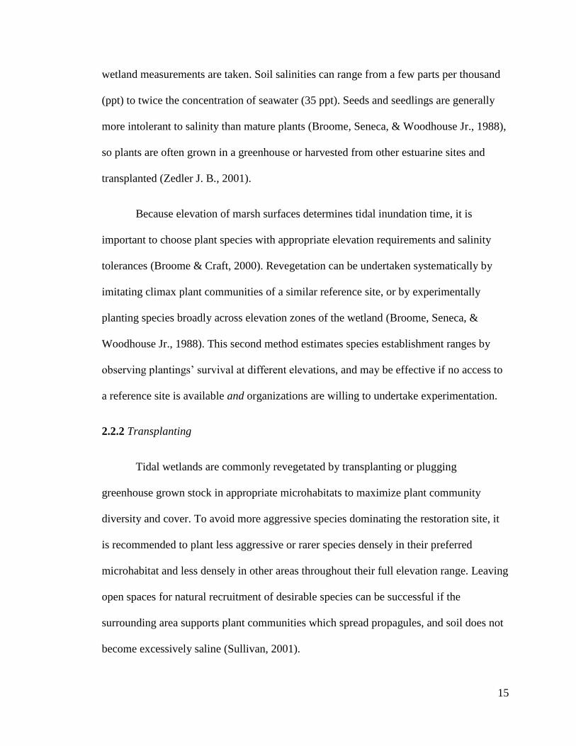
Figure 2.1 Aerial photo of Bayshore Preserve showing channels and

locations for each set of experimental plots.

29

3.3 Treatment Applications

Five different sowing treatments were applied:

• Unseeded control: no treatment

• Hydromulch only control: no seed

• Broadcast seeded + hydromulch (hereafter referred to as “seed +

hydromulch”)

• Broadcast seeded with burlap cover

• Broadcast seeded only

Figures 4.1 through 4.3 show layout of experimental plots in each channel, and

Tables 3.1 to 3.3 show associated treatments. Plots 1.1 and 2.1 were positioned across

from each other in every channel, closest to the channel terminus. Plots 1.5 and 2.5 are

closest to the bay in every channel.

Figure 3.1 Affixing polyethylene sheeting to plots during seeding preparation.

30

Plot Treatment

A1.1

Hydromulch

only control

A1.2

Seed +

hydromulch

A1.3 Burlap

A1.4 Seed only

A1.5

Unseeded

control

A2.1 Seed only

A2.2

Seed +

hydromulch

A2.3

Hydromulch

only control

A2.4

Unseeded

control

A2.5 Burlap

Plot Treatment

B1.1

Seed +

hydromulch

B1.2 Burlap

B1.3

Hydromulch

only control

B1.4 Seed only

B1.5

Unseeded

control

B2.1

Seed +

hydromulch

B2.2

Hydromulch

only control

B2.3 Seed only

B2.4

Unseeded

control

B2.5 Burlap

Figure 4.1 Plot layout in Channel A.

Figure 4.2 Plot layout in Channel B.

Table 3.1 Treatments

applied to each plot in

Channel A.

Table 3.2 Treatments

applied to each plot in

Channel B.

31

3.3.1 Unseeded control treatment

There was one unseeded control plot in each set of plots. This control treatment

was covered with polyethylene sheeting during the treatment application process.

3.3.2 Hydromulch only control treatment

One plot in each set received a hydromulch only control treatment. Adjacent plots

to this treatment were covered securely by polyethylene sheeting to avoid contamination.

Hydromulch was applied, by a contractor (Hoyt’s Hydroseeding, Tahuya, WA), two

inches deep to each hydromulch only treatment plot. The hydromulch product used was

Rainier Fiber™ Premium Wood Fiber Mulch For Hydroseeding and Erosion Control. See

Appendix A for details on hydromulch specifications and mixing instructions.

Plot Treatment

C1.1 Burlap

C1.2

Hydromulch

only control

C1.3 Seed only

C1.4

Seed +

hydromulch

C1.5

Unseeded

control

C2.1 Burlap

C2.2

Unseeded

control

C2.3

Hydromulch

only control

C2.4 Seed only

C2.5

Seed +

hydromulch

Figure 4.3 Plot layout in Channel C. Table 3.3 Treatments

applied to each plot in

Channel C.

32

3.3.3 Broadcast seed plus hydromulch treatment

One plot in each set received a broadcast seeding plus hydromulch cap treatment.

Plots adjacent to the area to be treated were covered using polyethylene sheeting and

nursery staples. The treated plot was broadcast seeded using the prepared seed mixture,

then covered by two inches (2”) of hydromulch by the contractor.

3.3.4 Broadcast seed plus burlap cover treatment

One plot in each set received a broadcast seeding plus burlap cover treatment.

Adjacent plots were covered to avoid contamination. Prepared seed mixture was

broadcast onto the treatment plot, and a 1x2 meter piece of burlap was tacked overtop the

plot.

3.3.5 Broadcast seed only treatment

One plot in each set received a broadcast seeding treatment. Again, adjacent plots

were covered to avoid contamination. Prepared seed mixture was broadcast onto the plot.

No covering or mulch of any kind was used to secure seeds in this treatment, nor were

seeds raked into the soil after application.

After all five treatments were applied, remaining polyethylene sheeting was

removed, and treatments were checked 24 hours later.

33

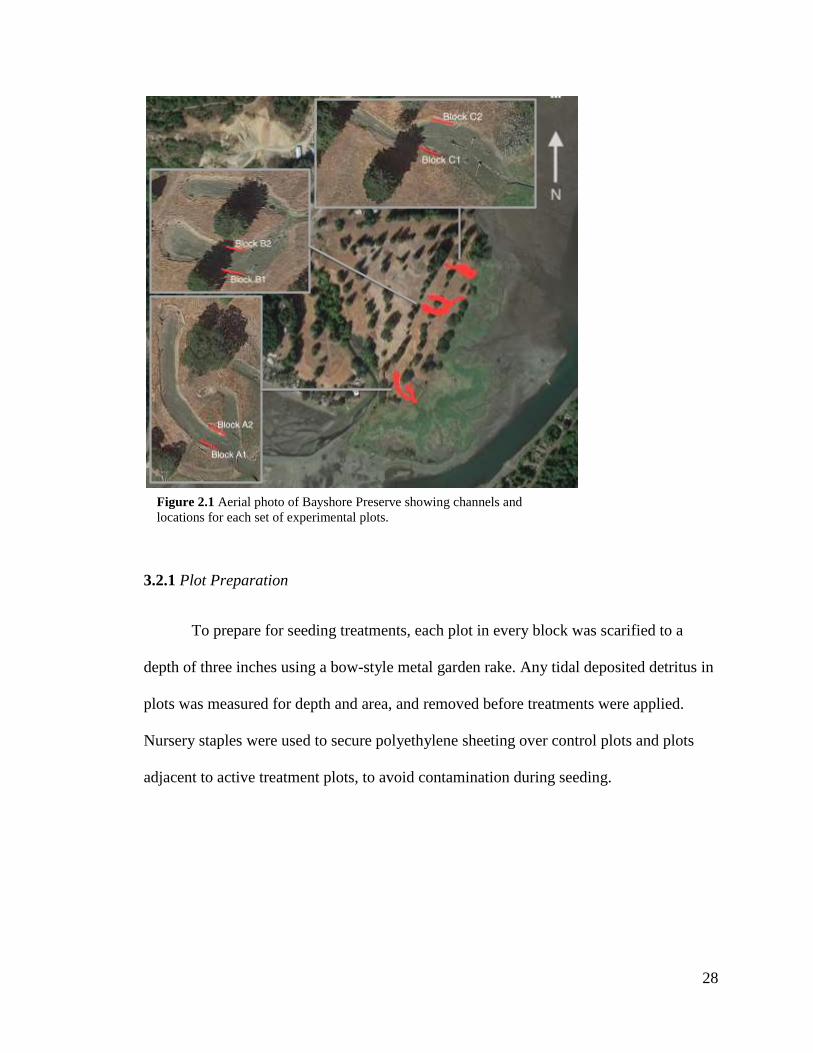
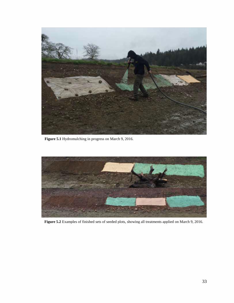
Figure 5.1 Hydromulching in progress on March 9, 2016.

Figure 5.2 Examples of finished sets of seeded plots, showing all treatments applied on March 9, 2016.

34

3.4 Plot Elevations

Elevations were measured at the midpoints of the top and bottom edges of each

plot using the standard method of differential leveling. To prepare, several benchmark

points near experimental channel edges were located using Google Maps and coordinates

were recorded. These benchmark point coordinates were input into the USGS Elevation

Point Query Service (NAD83) to retrieve point elevations in meters. A horizontal laser

level on a tripod was used to measure vertical differences in elevation of each plot’s top

and bottom edge, relative to the elevation of the benchmark point used.

The laser level was affixed to the tripod and set up so its height was just above

eye level, in a location where the line of sight allowed me to see the backsight and the

foresights. The instrument was leveled, making sure the bubble was within the circle on

Figure 5.3 Plots 24 hours after seeding on March 10, 2016. Note migration of hydromulch, especially

in plot at left. Hand broadcast sowing and hydromulching was performed on March 9, with hydromulch

applied between 9:00am and 10:00am (seed was applied prior, the same morning). Low tide occurred at

1:11pm at 2.58 feet (MLLW), and the next high tide occurred 6:22pm at 14.35 feet.

35

the tripod, and that the bubble was between the two lines on the laser level. The

instrument was moved 90 degrees to both sides to check leveling.

Using a handheld GPS device with benchmark coordinates input, we navigated to

and marked the benchmark elevation point. A reading was taken at the benchmark point

to determine elevation difference between the height of the instrument and the known

elevation—this is known as the backsight. The backsight rod reading value (BS) was

added to the known elevation value at the benchmark point—this gave us the height of

the instrument (HI) relative to the benchmark’s known elevation. From this point, we

took rod readings at the midpoint of each top and bottom edge of each plot—these were

the foresights (FS). To calculate elevation of each point, we subtracted the foresight

reading from the height of the instrument (i.e. HI-FS=elev). To end the survey, we

returned to the same benchmark point and took another reading to confirm the instrument

height had not deviated outside an acceptable margin of error (0.03m) (University of

Colorado Boulder, n.d.).

3.4.1 Calculating tidal inundation

To calculate how many tides completely inundated all experimental plots,

converting elevations from the horizontal datum (NAD83), in which original data was

collected using the USGS elevation benchmark points, into a vertical datum (NAVD88)

was required. Vertical datums are used to measure heights of various points relative to a

set zero elevation, and tides are often measured using Mean Lower Low Water (MLLW).

MLLW is the average elevation of the daily lower low tide over a 19-year recording

36

period (also known as the National Tidal Datum Epoch), relative to a primary benchmark

at the tidal station (NOAA, 2017).

Tide information was calculated based on the MLLW datum predictions for

Barron Point, Little Skookum Inlet Entrance (NOAA Subordinate Station ID 9446742)

located in Shelton, WA. Little Skookum station is referenced to Seattle (Station ID

9447130), so plot elevations were adjusted using NAVD88 referred to MLLW at this

Seattle location to calculate the total number of high tides that submerged the plots

between soil sample collection dates. See appendix Table A1 for a chart showing original

elevations collected in NAD83 and converted elevations to relative datums.

3.5 Soil Sampling

3.5.1 Collection

Soil samples were collected on March 4, 2016 from each plot to test for soil

salinity. In each plot, five six-inch deep scoops were collected from random locations and

mixed together in a clean bucket to create a composite sample. This composite sample

was screened through a large screen into a new clean bucket to remove rocks and debris.

The rocks and debris were discarded back into the tidal channel, below and not in the plot

the sample was taken from. Approximately one quarter pound of this soil was reserved

and placed into a new, labeled 1-quart ziplock bag. Any remaining soil was returned to

the sample holes in the plot. Before moving on to the next plot, buckets and the sieve

were wiped with a towel until clean, rinsed with distilled water, and dried with a separate

clean towel.

37

A second round of soil samples was collected on February 13-14, 2017 to

measure salinity changes across control plots’ elevation gradients. Composite samples

were collected from three locations along the elevation gradient in the unseeded control

plot in each block, 0.1, 0.5, and 0.9 meters from the top of each control plot. Three six-

inch deep scoops were collected from each elevation within the plot, mixed together, and

processed as above.

3.5.2 Drying

All first-round samples were air dried at room temperature by leaving ziplock

bags open and periodically shaking the samples to redistribute the soil until completely

dry. Second-round soil samples were dried in a drying oven, stirring periodically, at 90F

for 24-48 hours (or until completely dry) in paper bags.

3.5.3 Electrical conductivity testing for salinity

Each sample was subjected to soil electrical conductivity testing for soluble salts,

using a Hanna HI 9813-6 Portable pH/EC/TDS/C Meter. The meter was calibrated

before each testing session and after every tenth sample to a known electrical

conductivity standard using Hanna aqueous electrolyte calibration solution (HI 70031;

1413 S/cm) and temperature. Before testing began, each sample was sieved again

through a 2mm (U.S. #10) soil sieve and mixed well. A 1:5 extraction method was

used—20 grams of soil were measured and mixed with 100mL of distilled water in a

glass beaker. The solution was mixed well with a stainless steel lab spoon spatula for 30

seconds every five minutes, for 30 minutes. After the 30-minute mixing period, the

solution was allowed to rest for 30 minutes so fine sediment could settle. This solution

was strained through VWR Scientific 28213 Grade 617 (Fast) Qualitative filter paper into

38

a separate clean, dry beaker. The electrical conductivity in mS/cm (millisiemens per

centimeter) of this filtrate was read with the Hanna meter and recorded. Each sample was

retested in duplicate to determine sample variability.

3.6 Vegetation Establishment Monitoring

Experimental plots were monitored for vegetative germination and plant

establishment at low tide, once per month beginning one month after seeding. Monitoring

was conducted on the following dates: April 8, May 5, June 1, June 21, July 23, August

16, September 20-24, and October 20, 2016.

Qualitative observations were made at each visit regarding changes, patterns and

effects of tide on each type of plot; thickness of new litter and debris deposits; estimated

percent of hydromulch washed away; and development of plant communities in greater

tidal channel areas. Quantitative measurements taken included first germination dates of

observed species, density of each planted and naturally occurring species, and total

vegetative cover in each plot.

3.6.1 Sampling for density & percent cover

Using the PVC frame constructed for plot installation, 1 m2 sample areas were

delineated by running twine through pre-drilled holes and laying the frame over the rebar

plot corners. Species densities were measured by counting each live stem that occurred

within the 1m2 sample area—as a rule, stems were counted if they fell underneath the top

edge of the frame or right-side twine, and omitted if they fell underneath the bottom edge

of the frame or left-side twine. When estimating percent total vegetative cover, any and

39

all vegetative plant parts that fell within the sample area were counted, even if a plant’s

stem was itself outside of the sample area.

3.7 Germination Testing

Germination testing was performed on Atriplex patula to determine viability of

seed. A first germination test failed due to equipment malfunction, so a second test was

Figure 6.1 PVC frame and twine delineating 1m2 sample area. Top: Plot A2.5 Bottom: Plot A2.1.

40

performed to gain usable results. Due to time constraints, testing of A. patula seed was

prioritized based on occurrence of two Atriplex species in the experimental plots (see

Chapters 4 & 5).

Testing was performed in a controlled environment, under non-saline conditions.

Fresh (deionized) water was used to maximize the likelihood of germination—based on

measurements of environmental conditions on-site at the time of sowing, field conditions

in which sowing took place revealed close to freshwater soil salinity concentrations.

Before germination testing occurred, A. patula seeds underwent a period of cold-

moist stratification for 30 days (Baskin & Baskin, 2001). 100 seeds of A. patula were

wrapped in cotton gauze, moistened with distilled water, and wrapped in a paper towel

moistened with distilled water. This seed packet was put into a plastic bag and twist-tied

shut. Seeds were stratified in a dedicated refrigerator at a temperature of 38F.

Once the stratification period was complete, 100 A. patula seeds were separated

into five sterilized petri dishes (20 seeds per dish) lined with one piece of filter paper

(Double Rings 90mm) and 3mL of distilled water was added. Petri dishes were placed

into the germination chamber (SG30 Controlled Environment Chamber), and started on

the 12-hour dark cycle. Although Baskin & Baskin (2002) tested A. patula at a 5/25 °C

alternating temperature cycle, this test used a 5/20 °C setting with 12 hours of dark at 5°C

and 12 hours of grow lights (40 μmol photons m-2 s-1 PPFD) at 20°C. The decision to

lower the upper temperature resulted from a desire to test multiple species at once in the

interest of time.

41

During the germination testing period, each set of seeds was monitored for

germination (emergence of a radicle—the embryonic root). As seeds sprouted, successful

germinants were recorded for the day, and removed from the petri dish before returning

samples to the germination chamber. Seeds were monitored every other day for a period

of 35 days.

3.7 Data Analysis

Data was analyzed using JMP software. A one-way analysis of variance

(ANOVA) was performed on vegetative recruitment data to compare treatment effects on

planted species against two controls (unseeded control and unseeded hydromulch only

control). A two-tailed t-test was run to compare the treatment means to each other in

significant datasets.

Linear regression analysis was performed to reveal correlations between elevation

and species recruitment and richness on select dates. Continuous variables were plotted

against each other, and appropriateness of fit was checked by plotting residuals.

42

Chapter 4: Results

This chapter contains the vegetative survey analysis results, along with results of

soil salinity and germination testing. First, section 4.1 introduces Atriplex patula as the

sole successful species in this experiment and addresses reasons for plant identification

confusion that occurred in this experiment. Section 4.2 highlights overall species

occurrence in the tidal channels and discusses natural vegetative recruitment. In section

4.3, results showing A. patula recruiting with higher success in burlap and hydromulch

treatments are explained in detail by delving into results from each monitoring date.

Section 4.4 shows that naturally recruiting species did not show significant density

differences between treatment types, but did show an unusual relationship between

species richness and elevation. Increasing soil salinity and tidal inundation time are then

discussed in section 4.5. Finally, section 4.6 reveals germination test results showed that

four species tested were indeed viable, indicating their potential for germination in the

field.

Graphs in this section reflect results analyzed from six replicates of each

treatment. Oneway ANOVA graphs are set up as follows: x-axes are labeled with

manipulative treatment types, and y-axes represent the mean live stem densities recorded

for each treatment type. Linear regression graphs show species richness plotted against

elevation per plot in which data was collected on the date of highest richness.

4.1 Planted Species Germination and Establishment to Maturity

Of five planted species, one was positively identified to have reached maturity

within the experimental plots: Atriplex patula (Figure 7.1). This species was not

43

positively identified until June 2016—at the first two monitoring visits it was confused

with a naturally occurring species, Atriplex prostrata. Both species were counted

together—they were thought to be the same—and this is reflected in the data for the April

through May 2016 monitoring period. By June, distinctive differences in leaf shape

between the observed specimens prompted an in-depth identification effort, revealing that

two species were present in the experimental plots. Beginning in June, both distinct

Atriplex species are reflected in the data.1

1 Since completion of the experiment, a potential misidentification of the naturally occurring species

Atriplex prostrata has come to light. Based upon observations by Capitol Land Trust (CLT) ecologists, the

plant referred to in this study may in fact be Chenopodium album—which is difficult to distinguish from A.

prostrata to the naked eye. The plant in question was keyed to species A. prostrata in summer 2016,

however specimens were beginning to senesce and few intact flowers remained. This presents a problem of

ambiguous identification. Therefore, in the following sections, all mentions of A. prostrata could

potentially be referring to C. album—final identification of which species is present on-site will be

determined by CLT in 2017 when flowering specimens are present. This potential misidentification in no

way affects the data analysis or results, as only the planted Atriplex patula was analyzed for treatment

effects.

Figure 7.1 Recorded observations of each of five planted species within experimental plots.

44

4.2 Naturally Occurring Diversity in Tidal Channels

Several naturally recruited native species colonized the experimental plots (Figure

7.2) and the tidal channel areas that were not part of the experimental plots. All tidal

channel floors were abundantly vegetated by Salicornia virginica and Spergularia

canadensis, while Atriplex prostrata was commonly observed. In tidal Channel A,

Jaumea carnosa was less commonly observed, and Atriplex patula was rarely observed

on the channel floor in addition to species mentioned above. All tidal channel walls

supported A. prostrata (commonly observed), A. patula (common to less common), S.

virginica and Spergularia canadensis (both common to less common).

Channel A also supported the greatest species diversity on channel walls, with

common observations of A. prostrata, less common occurrences of A. patula (becoming

more common approaching experimental plots), Grindelia integrifolia, S. virginica

Figure 7.2 Recorded observations of naturally recruited (non-planted) species within experimental

plots.

45

(generally present on lower channel walls), and Spergularia canadensis, and rare

occurrence of J. carnosa. Two unidentified species occurred on tidal channel walls. One

appeared to be in the Cyperaceae or Poaceae families (species in these families exhibit

very similar structure at young growth stages), and occupied upper elevation areas in

some experimental plots (hereafter referred to as UNKN1; Figure 8.1). The other

(UNKN2; Figure 8.2) occurred near channel edges (one specimen each in Channel A &

B), having thick, fleshy leaves to eight inches long.

4.3 Atriplex patula Treatment Responses

Results seem to indicate a pattern showing higher A. patula stem densities in

treatments that were manipulated by adding seed. Beginning on June 1, 2016, we clearly

see higher recruitment rates in the seed + hydromulch and burlap treatment groups than

the control treatments. Plots which were dry broadcast seeded also exhibit a pattern of

higher plant establishment than controls, but less so than more intensely manipulated

plots.

Figure 8.1 (Left) Species UNKN1 occurred in experimental plots. Figure 8.2 (Right) Species

UNKN2 occurred outside of experimental plots on the edge of tidal channel.

46

Overall, the pattern seems to indicate that hydromulching or otherwise providing

a stabilizing fabric over this species after broadcast seeding onto the soil results in higher

rates of plant establishment. Higher numbers of planted A. patula in the first season after

saltwater reintroduction adds value by providing more aboveground biomass to the

system, increasing the ability of the channels to trap sediment, and a faster rate of habitat

development benefitting benthic macroinvertebrates and other species.

Figure 9.1 shows an overview of mean live stem densities of A. patula on each

sampling date for each treatment type. Results from each individual monitoring date are

discussed in more detail below.

47

4.3.1 April 8, 2016

On April 8, germinants of Atriplex spp. were observed in each treatment plot.

Because germinants were so young—most had cotyledons, some had developed one set

of true leaves—it was impossible to identify to species. Significant differences (p=.0045)

in germination were observed between treatment groups on this date.

Figure 9.1 Mean Atriplex species densities shown for each monitoring date. Graphs in red show data

gathered before A. patula was differentiated from A. prostrata, and therefore simply reflect mean

densities of Atriplex spp. Note that over time, stem densities are clearly higher in plots that received

the hydromulch-over-seed and burlap treatments.

48

A two-tailed t-test showed that Atriplex spp. germinated in significantly greater

numbers in the seed + HM plot. The seed + HM group had a sample mean (x̄) of 7.33

germinants, significantly higher (p=.0019) than the unseeded control (x̄=.873). The

hydromulch only control group (hereafter referred to as “HM”) exhibited a sample mean

of 4.33 germinants per plot. The burlap and seed only treatment groups had much lower

germinant counts, and were both significantly lower (p=.0030 and .0012, respectively)

than the seed + HM group on this date. The burlap treatment resulted in x̄=1.67

germinants. The seed only treatment resulted in x̄=.50 germinants. No significant

differences were observed between the unseeded control and either the burlap (p=.8604)

or the seed only (p=.8604) treatment groups.

Figure 10.1 4/8/16 Establishment of Atriplex spp. in seed +

hydromulch, burlap, and seed only treatment plots—compared with

unseeded control and unseeded hydromulched control treatments.

49

4.3.2 May 5, 2016

By this date, highly significant differences (p<.0001) are seen between treatment

groups for Atriplex spp. At this point, Atriplex spp. were at a young stage of maturation,

with most plants showing several sets of true leaves and no flowers. While noticeable

differences in leaf shapes of Atriplex plants were observed, they weren’t distinct enough

to prompt investigation into the possible presence of two “varieties.” Therefore, at this

date, all Atriplex spp. were again counted and analyzed together.

When performing a two-tailed t-test, the sample means of all seeded treatments

reflected significantly greater numbers of Atriplex spp. germination and establishment

compared with the two controls. The sample mean of the burlap treatment (x̄=15.00) is

significantly higher than the unseeded (p=.0001, x̄=5.17) and HM (p=.0002, x̄=5.67)

control groups. The seed + HM treatment also exhibited significantly higher germination

and establishment of Atriplex spp. (x̄=14.00) compared with the unseeded (p=.0004) and

HM (p=.0007) controls. The seed only treatment exhibited a sample mean (x̄=10.83)

significantly higher than the unseeded (p=.0143) and HM (p=.0241) controls. There were

no significant differences detected between the seed only and burlap (p=.0641) or seed +

HM (p=.1534) groups. No significant differences were observed between the unseeded

and HM control groups (p=.8181).

50

4.3.3 June 1, 2016

This is the first date in which data reflects positive identification of Atriplex

patula and Atriplex prostrata as two separate species, both occurring in the experimental

plots. For the first two data collection dates, this distinction was not confirmed and all

Atriplex species within the sample area were counted together. On this date, a oneway

analysis of variance (ANOVA) showed significant differences (p<.0001) in A. patula live

stem densities between treatment groups.

A two-tailed t-test showed significantly higher live stem counts in all seeded

treatments. The seed + HM group had a significantly higher number of established plants

Figure 10.2 5/5/16 Establishment of A. patula in seed + hydromulch,

burlap, and seed only treatment plots—compared with unseeded control

and unseeded hydromulched control treatments.

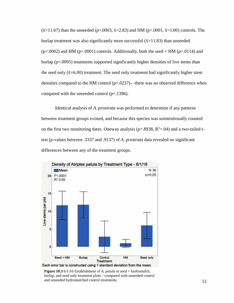
51

(x̄=11.67) than the unseeded (p=.0003, x̄=2.83) and HM (p<.0001, x̄=1.00) controls. The

burlap treatment was also significantly more successful (x̄=11.83) than unseeded

(p=.0002) and HM (p<.0001) controls. Additionally, both the seed + HM (p=.0114) and

burlap (p=.0095) treatments supported significantly higher densities of live stems than

the seed only (x̄=6.00) treatment. The seed only treatment had significantly higher stem

densities compared to the HM control (p=.0237)—there was no observed difference when

compared with the unseeded control (p=.1396).

Identical analysis of A. prostrata was performed to determine if any patterns

between treatment groups existed, and because this species was unintentionally counted

on the first two monitoring dates. Oneway analysis (p=.8938, R2=.04) and a two-tailed t-

test (p-values between .3337 and .9137) of A. prostrata data revealed no significant

differences between any of the treatment groups.

Figure 10.3 6/1/16 Establishment of A. patula in seed + hydromulch,

burlap, and seed only treatment plots—compared with unseeded control

and unseeded hydromulched control treatments.

52

4.3.4 June 21, 2016

Oneway analysis revealed significant differences (p<.0001) between stem

densities of A. patula across treatment groups. Two-tailed t-tests showed significant

differences between the seed + HM treatment (x̄=11.67) compared with unseeded

(p=.0003, x̄=2.83) and HM (p<.0001, x̄=1.00) controls. The burlap treatment recruited

significantly higher live stem densities (x̄=12.33) than unseeded (p=.0001) and HM

(p<.0001) controls. The seed only treatment group exhibited higher stem densities

(x̄=6.67) than only the HM (p=.0133) control group—when compared with unseeded

controls no significant difference was detected (p=.0834). The seed only treatment

densities were additionally significantly lower than seed + HM (p=.0268) and burlap

(p=.0133) treatments.

A. prostrata showed no significant differences between treatment groups

(p=.8490, R2=.05).

53

4.3.5 July 23 and August 16, 2016

On July 23 and August 16, 2016 monitoring dates, A. patula continues to show

significant differences between treatments (p<.0001). On respective dates, the seed + HM

treatments show significantly higher stem densities (x̄=10.67 on both dates) than

unseeded (p=.0002 on 7/23/16, p=.0017 on 8/16/16) and HM (p=.0002 on 7/23/16,

p=.0002 on 8/16/16) controls. Burlap treatments show significantly higher stem densities

(x̄=12.33 on 7/23/16, x̄=12.83 on 8/16/16) than unseeded (p=.0002 on 7/23/16, p=.0001

on 8/16/16) and HM (p<.0001 on both dates) controls. Seed only treatment densities

Figure 10.4 6/21/16 Establishment of A. patula in seed + hydromulch,

burlap, and seed only treatment plots—compared with unseeded control

and unseeded hydromulched control treatments.

54

(x̄=6.50 on both dates) continue to only be significantly higher than HM controls

(p=.0185 on 7/23/16, p=.0205 on 8/16/16).

A. prostrata continues to show no significant differences between treatment

groups (p=.8761, R2=.05 on 7/23/16 and p=.8591, R2=.05 on 8/16/16).

Figure 10.5 7/23/16 Establishment of A. patula in seed + hydromulch,

burlap, and seed only treatment plots—compared with unseeded control

and unseeded hydromulched control treatments.

55

4.3.6 September 24, 2016

Again, ANOVA reveals significant differences in live stem densities of A. patula

(p=.0001) between treatment groups. Two-tailed t-tests show greater seed + HM

treatment stem densities (x̄=12.67) than unseeded (p=.0017, x̄=3.00) and HM (p=.0003,

x̄=1.00) controls. Burlap treatments also achieved significantly higher stem densities

(x̄=14.50) than unseeded (p=.0003) and HM (p<.0001) controls. Seed only plots continue

to show lower stem densities (x̄=6.83) than the previous two treatments (p=.0437 and

.0099, respectively). Seed only treatments again are only higher than HM controls

(p=.0437).

Figure 10.6 8/16/16 Establishment of A. patula in seed + hydromulch,

burlap, and seed only treatment plots—compared with unseeded control

and unseeded hydromulched control treatments.

56

ANOVA reveals no significant differences in A. prostrata stem densities between

treatments (p=.8832, R2=.04).

4.3.7 October 20, 2016

On this date most plants were almost fully senesced (dying, or entering

dormancy). Plants were counted if they exhibited signs of life—dry, dead specimens were

ignored. ANOVA showed significant differences between treatments (p=.0007). The

burlap treatment contained significantly higher live stem densities (x̄=5.33) than all other

treatment types on this date. Two-tailed t-tests confirmed this when compared with

unseeded controls (p=.0003, x̄=.83), HM controls (p<.0001, x̄=.33), seed + HM (p=.0187,

x̄=2.67), and seed only (p=.0131, x̄=2.50) treatments. The seed + HM treatment still

Figure 10.7 9/24/16 Establishment of A. patula in seed +

hydromulch, burlap, and seed only treatment plots—compared with

unseeded control and unseeded hydromulched control treatments.

57

exhibited higher live stem densities than HM controls (p=.0372), but was not

significantly different from the unseeded controls (p=.0962) on this date.

A. prostrata again shows no significant differences between treatments (p=.7359,

R2=.07).

4.4 Natural Recruitment in Experimental Plots and Treatment Effects

4.4.1 Stem densities across treatments

Naturally recruited species colonized the experimental plots, and live stem counts

were performed during data collection. Two species (Salicornia virginica and

Figure 10.8 10/20/16 Establishment of A. patula in seed + hydromulch,

burlap, and seed only treatment plots—compared with unseeded control and

unseeded hydromulched control treatments. Lower densities reflect end of

season plant senescence and die-off.

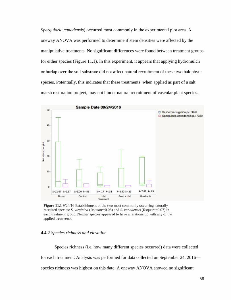
58

Spergularia canadensis) occurred most commonly in the experimental plot area. A

oneway ANOVA was performed to determine if stem densities were affected by the

manipulative treatments. No significant differences were found between treatment groups

for either species (Figure 11.1). In this experiment, it appears that applying hydromulch

or burlap over the soil substrate did not affect natural recruitment of these two halophyte

species. Potentially, this indicates that these treatments, when applied as part of a salt

marsh restoration project, may not hinder natural recruitment of vascular plant species.

4.4.2 Species richness and elevation

Species richness (i.e. how many different species occurred) data were collected

for each treatment. Analysis was performed for data collected on September 24, 2016—

species richness was highest on this date. A oneway ANOVA showed no significant

Figure 11.1 9/24/16 Establishment of the two most commonly occurring naturally

recruited species: S. virginica (Rsquare=0.08) and S. canadensis (Rsquare=0.07) in

each treatment group. Neither species appeared to have a relationship with any of the

applied treatments.

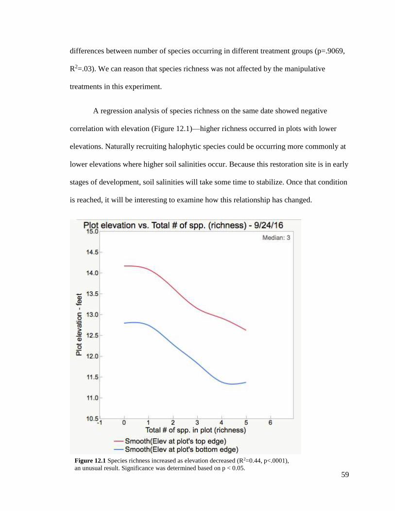
59

differences between number of species occurring in different treatment groups (p=.9069,

R2=.03). We can reason that species richness was not affected by the manipulative

treatments in this experiment.

A regression analysis of species richness on the same date showed negative

correlation with elevation (Figure 12.1)—higher richness occurred in plots with lower

elevations. Naturally recruiting halophytic species could be occurring more commonly at

lower elevations where higher soil salinities occur. Because this restoration site is in early

stages of development, soil salinities will take some time to stabilize. Once that condition

is reached, it will be interesting to examine how this relationship has changed.

Figure 12.1 Species richness increased as elevation decreased (R2=0.44, p<.0001),

an unusual result. Significance was determined based on p < 0.05.

60

4.5 Soil Salinity

Soil salinity in all experimental plots was sampled on March 4, 2016 and fell

within the freshwater range, below 0.5 ppt. In fact, all soil samples except for one—plot

C1.3—tested below 0.1 ppt. A second sample was taken on February 14, 2017. These

results showed an increase in soil salinity in the unseeded control plots—all samples fell

between 0.5 and 0.75 ppt. See chart below (Figure 13.1) comparing soil salinity levels on

the two sample dates.

Salt content is expressed in parts per thousand (ppt).

o 0.0 to 0.5 ppt = fresh water

o 0.6 to 30 ppt = brackish water

o >30 to 50 ppt = saline

o Seawater = 35 ppt

o Drinking water supply generally restricted to <0.5 ppt.

o Irrigation water must be less than 2 ppt or it will kill most crop plants.

61

4.5.1 Elevation and tidal inundation

After conversion to the Mean Lower Low Water (MLLW) datum, all plots fell

between 8.48 and 12.12 feet in elevation. Using NOAA Tide Predictions charts from

2016 and 2017, each high tide above 12.1 feet was counted for Barron Point, Little

Skookum Inlet Entrance tide station (Station ID 9446742) between the dates of 3/9/2016

and 2/14/2017. Between these two dates it was estimated that 530 high tide events

completely submerged all experimental plots. As the new tidal channels were exposed to

these tides, allowing seawater to absorb into the substrate, soil salinities rose (Figure

13.1). Soil salinities should be expected to continue rising over time until they stabilize.

As soil becomes more saline, plant community compositions should shift toward

vegetation types reflected in mature salt marshes.

Figure 13.1 Soil salinity levels measured by electrical conductivity in

parts per thousand (ppt). Samples in green were collected from the

unseeded control plots.

62

4.6 Germination Test Results

A germination test of A. patula resulted in 83% of the seeds germinating quite

rapidly—at 20°C germination began within 24 hours, peaked at four days, and ceased

altogether after 11 days in the chamber. After 11 days, the temperature was raised to

25°C because A. patula germination was assumed to be nearly complete. At the

conclusion of the germination test on 5/17/17, Carex lyngbyei and Carex obnupta showed

low germination rates in freshwater conditions (3% and 8%, respectively), while

Schoenoplectus americanus germinated at 41%.

63

Chapter 5: Discussion

5.1 Hydromulching onto Broadcast Seed—Success with Atriplex patula

Data from this experiment show a pattern potentially indicating a relationship

between Atriplex patula plant establishment and the hydromulch treatment applied over

broadcast seed. The oneway ANOVA for this species showed statistically significant

differences of means between the six hydromulched samples and six unseeded control

samples, for all monitoring dates. This may be promising for future restorations of tidal

wetlands in which direct seeding of this species is desired. This species could be

broadcast seeded mechanically or by hand during an ebb tide, and hydromulch applied

directly after. The other four species did not yield results in this study. This could be due

to several factors, which will be discussed in subsequent sections.

5.1.1 Identification difficulties of Cyperaceae species

The four species for which no data was collected were all in the Cyperaceae

family. Species in this family are quite challenging to identify when very young, and can

easily be confused with germinating grasses (Poaceae family). When graminoids present

as germinants, it is very difficult to distinguish between key vegetative identification

features such as stem shape and whether leaf sheaths are open or closed (Chase, Clark, &

Pohl, 1996; Carex Working Group, 2014)—and of course floral features are lacking.

Germinants were observed on several monitoring dates that may have been species

belonging to either the Cyperaceae or Poaceae families. Because of their young age,

identification to family was not determined.

64

While these plants in question appear on the first two monitoring dates, they had

disappeared by June 2016, and did not reappear in experimental plots until August. It is

speculated that unusually hot weather could have caused spring die-off of these

germinants, drying and heating the soil beyond what the tender seedlings could handle.

Perhaps a second, late emergence of germinants occurred that would account for the

period with no observations. Temperatures reached the mid to high-eighties (°F) during a

four-day period in mid-April, and in the first week of May temperatures rose to a record

high of 97°F by 5/5/16. Germinants were noted on that date, but subsequently were

absent until observed again starting on 8/16/16. Temperatures between May and August

ranged generally between 60°F and 89°F, with three temperature events above 90°F for

two or more days in a row during this time. Historical weather observations are based on

readings from Sanderson Field in Shelton, WA (Weather History for KSHN, 2016).

5.1.2 Seed limitations

Quality of seeds and sourcing locations are critically important in restoration.

Ideally, seed should be sourced as closely as geographically possible to the restoration

site. This maintains local genetic diversity and is critical in avoiding propagation of

genetic bottlenecks across the region. Seeds for this experiment were sourced from Inside

Passage Seeds, a specialty native seed company focused on providing seeds from the

Salish Sea bioregion and coastal areas ranging north and south. A. patula, C. lyngbyei,

and C. obnupta were all collected within Jefferson County, Washington. Eleocharis

palustris and Schoenoplectus americanus were collected in Benton and Lane Counties,

Oregon, respectively.

65

Beyond seed quality, age and storage conditions can affect viability. Seed for this

experiment were used within a month of receipt from Inside Passage Seeds, however seed

used for the germination test had been stored for a year in cool, dark and dry conditions.

Many species lose the ability to germinate as time passes or if exposed to high

temperatures, but not all. Because four out of the five planted species were not observed

during the first growing season at Bayshore Preserve, seeds were tested for viability in a

germination chamber under controlled conditions. E. palustris was excluded from testing

because it required temperatures above 27°C (Bartow, 2007) to germinate in a reasonable

amount of time. A. patula seeds tested were from a more recently collected (2016) lot

than seed used in the hydromulching experiment (collected 2015), and both lots were

collected from the same location (Shomer, 2016).

5.1.3 Controlled versus natural environments and seed germination

While germination testing can show whether seeds are viable or not, it is

important to note that the controlled environment of a germination chamber eliminates

several factors present in natural environments. During this test, seeds received

consistently adequate moisture throughout their germination phase and a non-variable

light and temperature regime. Seeds were not subject to potential stressors like pests,

pathogens, variable temperature and moisture inputs, tidal movement, or soil salinity

fluctuations. All of these factors can impede germination in the field, and this test merely

shows whether seeds of each species had the potential to germinate in the tidal channels.

The high rate (83%) of germination achieved for A. patula in controlled

conditions reflects results in which Baskin & Baskin achieved rapid germination of the

66

species (2001). The seed lot used in our germination test was collected in 2016. The

remaining lots of other species were collected in 2015. S. americanus achieved a 41%

germination rate, while C. lyngbyei germinated at 3% and C. obnupta germinated at 8%.

Because these three species were stored one year longer than A. patula, their viability

could have been reduced. Additionally, factors such as heat exposure during transport

may have reduced viability. Germination tests were conducted 12 months after the field

experiment was installed, introducing a potential decrease in viability over this time.

While seed viability is generally expected to decrease over time, these seeds

showed at least low levels of germination. These seeds were exposed to salinity stress—

even though within their expected tolerance ranges—and other environmental factors

immediately upon planting. As discussed, natural conditions make successful

germination a gamble, and it seems the conditions on-site were less than perfect for all

but A. patula seeds.

5.2 Atriplex spp. Treatment Responses

Though A. patula and A. prostrata were recorded as one species in early data

collection2, this mishap does begin to illuminate some interesting trends. The first

monitoring date shows two plots supporting high numbers of Atriplex germinants: seed +

hydromulch and the hydromulch only control groups. All the other treatments show very

little germination on the first date (4/8/16). The second monitoring date (5/5/16) shows

the hydromulch only control group supporting about the same amount of Atriplex spp.

plants, but the numbers rise significantly for all the other treatments. On 6/1/16, when A.

patula was positively identified and recorded separately from A. prostrata, we see the A.

2 See footnote 1, section 4.1 for information regarding ambiguous identification of A. prostrata.

67

patula density in the seed + hydromulch and burlap treatments decrease somewhat, along

with a notable decrease in the two control and seed only treatments. This general pattern

persists throughout the data collection period for A. patula. Since we see the density

numbers drop so drastically after A. prostrata was omitted, one could assume that the

hydromulch only control plot supported more of this naturally recruiting species at the

beginning of the season. Perhaps the hydromulch offered a more hospitable environment

for seeds already present in the seed bank to germinate—potentially by retaining soil

moisture during low tides (NRCS, 2003).

The A. patula density pattern reflected across the monitoring period shows the

highest recruitment in the burlap rather than the seed + hydromulch treatment. Although

the burlap treatment group did not show much germination at all on the first monitoring

date, from May on it supported a higher density of plants than any other treatment. It is

possible that the burlap itself may have slowed germination of Atriplex, blocking out

light. It is likely, however, that small germinants were simply not observed in April

because they were still underneath the fabric, and had emerged through by May. Overall,

there was not a significant difference in the densities of A. patula that were supported

between the burlap and seed + hydromulch treatments. Either way, both of the treatments

did a good job of increasing the ability of Atriplex patula to establish, compared with the

seed only treatments in the tidal channels. The USDA Natural Resource Conservation

Service recommends mulch usage when seeding for most types of restoration projects,

stating that they “reduce seed movement, mortality and predation, retain soil moisture

and fertilizers, and reduce erosion (2003).” From the results attained in this experiment, it

seems both types of “mulch” did a good job and it would be worth repeating the

68

experiment with other species, while calculating costs per square foot to determine the

most cost-effective method.

5.3 Recommendations

Repeating this experiment with A. patula and other species is recommended. At

Bayshore Preserve, second season (and beyond) data collection should determine

survivability of A. patula past the first growing season to determine if this planting

method augments longer-term development of the tidal wetland restoration—data should

be compared with reference plots in areas of the tidal channels that did not receive these

experimental treatments. An additional recommendation is identification of nursery

grown stock of Inside Passage’s A. patula seed to positively ensure that data collected

was indeed from planted seed (specimens are being grown at the time of this writing). In

the future, if possible, it may be desirable to grow seed stock to maturation prior to

experimentation to ensure positive species identification.

With future research of this method, it will be interesting to more closely study

influential factors (precipitation, extreme tides, elevation, aspect, etc.) on hydromulch

treatments more closely. For example, stratifying samples at different micro-elevations

could provide finer resolution data regarding species recruitment and secondary effects of

the hydromulch treatment on the soil substrate. It also seems wise to analyze chemical

and physical effects of hydromulch on seawater to determine any potentially detrimental

changes to water quality caused by this method. Monitoring soil development, benthic

invertebrates, and performing fish counts in treated areas compared to reference sites

would provide additional information related to functional development of revegetated

69

tidal wetlands, and aid in determining whether the methods are cost-effective into the

future of the restoration site.

70

Conclusion

Estuaries are an essential part of earth’s biosphere, providing unique habitat that

once sustained fisheries, ecosystem services for humans such as flood mitigation, and

critical habitat for wildlife. Estuary restoration efforts have increased since the

establishment of the National Estuary Program, authorized by the Clean Water Act in

1987. The science of estuary restoration has evolved over the years, with many

techniques developed and adaptively managed as scientists learn more about this

dynamic ecosystem.

Revegetation techniques such as direct seeding have often produced less than

ideal results, and producing plugs in a nursery and planting out can be costly. This thesis

researched a novel method to amend direct seeding techniques—hydromulching on top of

seeded areas to provide stabilization and buffer seed migration from tidal influence, with

hopes to gain higher revegetation establishment than with direct seeding alone. Our

hypothesis that hydromulch “seed anchoring” would increase germination and

establishment for five native saltmarsh species was not fully substantiated. Only one of

the planted species, Atriplex patula, was observed to have significantly greater

establishment in this experiment. None of the planted Cyperaceae family species were

positively identified as germinants or established plants during the course of this

experiment.

Natural recruitment of several native saltmarsh species did occur in the first year

post-dike removal time period in which this experiment took place. Prior estuary

restoration researchers have often recommended allowing natural vegetation regeneration

to occur instead of manipulating restoration sites, and long-term studies have shown

71

return of healthy ecosystem functioning without extra effort. However, if restoration

biologists or organizations desire specific plant communities and have the resources to do

some experimentation, this method could be worthy of continued research study. If found

to be successful with certain plant species, hydromulching could provide a quick and easy

revegetation method and allow organizations to stretch their project dollars to be as

effective as possible.

72

Works Cited

AOSA. (2007, April). Suggested purity and/or germination testing methods for species

without AOSA Rules testing procedures. Washington, DC: Association of

Official Seed Analysts. Retrieved from Association of Official Seed Analysts.

Barbier, E. B., Hacker, S. D., Kennedy, C., Koch, E. W., Stier, A. C., & Silliman, B. R.

(2011). The value of estuarine and coastal ecosystem services. Ecological

Monographs, 81(2), 169-193.

Bartow, A. (2007). Propagation protocol for production of Propagules (seeds, cuttings,

poles, etc.) Eleocharis palustris Roemer & J.A. Schultes seeds . Retrieved from

Native Plant Network Propagation Protocol Database: Protocol Information:

https://npn.rngr.net/renderNPNProtocolDetails?selectedProtocolIds=cyperaceae-

eleocharis-3454

Baskin, C. C. (2003). Native Plant Network. Retrieved November 10, 2015, from

nativeplantnetwork.org

Baskin, C. C., & Baskin, J. M. (2001). Seeds: Ecology, Biogeography, and Evolution of

Dormancy and Germination. San Diego: Academic Press.

Baskin, J. M., & Baskin, C. C. (2002). Propagation protocol for production of Container

(plug) Atriplex patula L. plants. Retrieved November 10, 2015, from Native Plant

Network: http://www.nativeplantnetwork.org

Bishop, G., & Bunter, W. (1999, June). PM Technical Note No. 5 (Rev. 2): BASIC

SEED DATA SUPPORTING NRCS VEGETATIVE GUIDES . CA: Natural

Resources Conservation Service, U.S. Department of Agriculture.

Boyer, K. B., & Zedler, J. B. (1998). Effects of nitrogen additions on the verical structure

of a constructed cordgrass marsh. Ecological Applications, 8, 692-705.

Boyer, K. B., & Zedler, J. B. (1999). Nitrogen addition could shift plant community

composition in a restored California salt marsh. Restoration Ecology, 7, 74-85.

Brennan, J. S. (2007). Marine riparian vegetation communities of Puget Sound.

Washington Sea Grant. Retrieved from

http://www.pugetsoundnearshore.org/technical_papers/riparian.pdf

Britz, R. H., & Eubel, C. A. (2003, December 15). People of the Water: A Curriculum on

the History and Culture of the Squaxin Island Tribe (Master's Thesis). Olympia,

Washington, United States: The Evergreen State College.

Broome, S. W. (1990). Creation and restoration of tidal wetlands in the southeastern

United States. In J. E. Kusler, & M. E. Kentula (Eds.), Wetland creation and

restoration: the status of the science (pp. 37-72). Washington, D.C.: Island Press.

Broome, S. W., & Craft, C. B. (2000). Tidal salt marsh restoration, creation, and

mitigation. In R. I. Barnhisel, W. L. Daniels, & R. G. Darmody (Eds.),

Reclamation of drastically disturbed lands (pp. 939-959). Madison: American

Society of Agronomy.

Broome, S. W., Seneca, E. D., & Woodhouse Jr., W. H. (1988). Tidal salt marsh

restoration. Aquatic Botany, 32, 1-22.

Buchanan, J. B. (2006). Nearshore birds in Puget Sound. Seattle: U.S. Army Corps of

Engineers.

73

Buenning, J. (2011, April 20). Plant Propagation Protocol for Carex lyngbyei. Retrieved

from Propagation Protocols for Pacific Northwest Plants:

https://courses.washington.edu/esrm412/protocols/protocols.htm

Capitol Land Trust. (2014, January 10). Bayshore Preserve Management Plan. Olympia,

WA, United States.

Capitol Land Trust. (2014, May 30). Capitol Land Trust Newsroom. Retrieved November

10, 2015, from Capitol Land Trust:

http://www.capitollandtrust.org/documents/CapitolLandTrustConservesHighestPr

iorityOaklandBayProperty.pdf

David, A. T., Ellings, C. S., Woo, I., Simenstad, C. A., Takekawa, J. Y., Turner, K. L., . .

. Takekawa, J. E. (2014). Foraging and growth potential of juvenile chinook

salmon after tidal restoration of a large river delta. Transactions of the American

Fisheries Society, 143, 1515-1529.

Deegan, D. (1959, October 8). Dr. Deegan's History of Mason County, Chapter 4.

Retrieved February 28, 2017, from Newspaper Archive of Shelton Mason County

Journal:

http://smc.stparchive.com/Archive/SMC/SMC10081959P15.php?tags=dr.|deegan

%27s

DeFrank, J., & Baldos, O. (2007). Assessing three hydroplanting techniques for

establishing Fimbristylis cymosa R.Br., a native Hawaiian Sedge. University of

Hawaii, Department of Tropical Plant and Soil Science. Hoolehua: USDA Natural

Resource Conservation Service.

Frenkel, R. E., Boss, T., & Schuller, S. R. (1978). Transition zone vegetation between

intertidal marsh and upland in Oregon and Washington. U.S. E.P.A. Report

(Grant No. R804963-01).

Fresh, K. L. (2006). Juvenile Pacific Salmon in Puget Sound. Puget Sound Nearshore

Partnership Report No. 2006-06. Seattle: Seattle District, U.S. Army Corps of

Engineers.

Gallego Fernandez, J. B., & Novo, F. G. (2007). High-intensity versus low-intensity

restoration alternatives of a tidal marsh in Guadalquivir estuary, Spain. Ecologcial

Engingeering(30), 112-121.

Gilbert, O. L., & Anderson, P. (1998). Habitat creation and repair. New York: Oxford

University Press.

Gill, S. J. (1983). Ethnobotany of the Makah and Ozette People, Olympic Peninsula,

Washington (USA). (Ph.D. Thesis). Washington State University.

Grabau, M. R., Milczarek, M. A., Kapiscak, M. M., Raulston, B. E., Garnett, G. N., &

Bunting, D. P. (2011). Direct seeding for riparian tree re-vegetation: Small-scale

field study of seeding methods and irrigation techniques. Ecological Engineering,

37, 864-872.

Gunther, E. (1973). Ethnobotany of western washington: the knowledge and use of

indigenous plants by native americans. Seattle, WA, United States: University of

Washington Press.

Guthrie, C. (2014, January 10). Bayshore Preserve Management Plan. Capitol Land

Trust. Olympia: Capitol Land Trust.

74

Hanslin, H. M., & Eggin, T. (2005, March). Salinity tolerance during germination of

seashore halophytes and salt-tolerant grass cultivars. Seed Science Research,

15(1), 43-50.

Harwell, A. (2014, May 15). Plant Propagation Protocol for Schoenoplectus pungens

(Vahl) Palla. Retrieved from Propagation Protocols for Pacific Northwest Plants:

https://courses.washington.edu/esrm412/protocols/protocols.htm

Houghton, J. P., & Ehlig, L. (2003). 2003 Georgia Basin/Puget Sound Research

Conference. A Tidal Habitat Restoration Success Story—The Union Slough

Restoration Project (p. 15). Edmonds: Pentec Environmental.

Howard, F. (1949). An Archaeological Site Survey of Southern Puget Sound. University

of Washington, Department of Anthropology. Seattle: Department of

Archaeology and Historic Preservations WISAARD database.

Jolivette, S. A., Huber, E. K., Van Galder, S. J., Foster, R., & Henry, M. (2014). Cultural

Resources Survey for the Capitol Land Trust Oakland Bay Estuary Conservation

Project, Phase III, Bayshore, Mason County, Washington. Capitol Land Trust.

Lacey: Statistical Research, Inc.

Keammerer, H. B. (2011, March). Community structure, plant interactions, seedling

performance and seed bank composition of salt marshes along an estuarine

gradient in Coos Bay, Oregon (Dissertation). Eugene, OR, United States:

University of Oregon.

Keefe, C. W. (1972, March). Marsh production: a summary of the literature. Science, 16,

163-181.

Kenny, S. (2007, August 16). Oakland Bay Action Plan. Retrieved February 27, 2017,

from Mason County Public Health:

https://www.co.mason.wa.us/forms/Env_Health/oakland_bay_plan.pdf

Knudson, P., & Woodhouse, J. W. (1982). Pacific Coastal Marshes. In R. R. Lewis (Ed.),

Creation and Restoration of Coastal Plant Communities (pp. 111-130). Boca

Raton, Florida: CRC Press.

Kruckeberg, A. R. (1991). The natural history of Puget sound country. Seattle:

University of Washington Press.

Kuhn, N., & Zedler, J. B. (1997). Differential effects of salinity and soil saturation on

native and exotic plants of a coustal salt marsh. Estuaries, 20, 391-403.

Mason Conservation District. (2004). Salmon habitat protection and restoration plan for

Water Resource Inventory Area 14, Kennedy-Goldsborough. Shelton: Mason

Conservation District.

Matthews, G. A., & Minello, T. J. (1994). Technology and success in restoration,

creation, and enhancement of Spartina alterniflora marshes in the United States.

Silver Spring: NOAA coastal Ocean Office.

Mazer, G., Booth, D., & Ewing, K. (2001). Limitations to vegetation establishment and

growth in biofiltration swales. Ecological Engineering, 17, 429-443.

Minello, T. J., Zimmerman, R. J., & Medina, R. (1994). The importance of edge for

natant macrofauna in a created salt marsh. Wetlands, 14, 184-198.

NOAA. (2008, March 25). Monitoring Estuaries. Retrieved from Estuaries:

http://oceanservice.noaa.gov/education/kits/estuaries/estuaries10_monitoring.html

NOAA. (2017, March 16). Vertical Datums. Retrieved from National Geodetic Survey:

https://www.ngs.noaa.gov/datums/vertical/

75

NRCS. (2005). TECHNICAL NOTES: Plant Materials - 6. Natural Resource

Conservation Service. Spokane: U.S. Department of Agriculture.

Peck, M. A., Fell, P. E., Allen, E. A., Gieg, C. R., Guthke, C. R., & Newkirk, M. O.

(1994). Evaluation of tidal marsh restoration: comparison of selected

macroinvertebrate populations on a restored impounded marsh valley and an

unimponded valley marsh within the same salt marsh system in Connecticut,

USA. Environmental Management, 18, 183-293.

Pojar, J., & MacKinnon, A. (1994). Plants of the Pacific Northwest Coast: Washington,

Oregon, British Columbia & Alaska. Vancouver, British Columbia, Canada: Lone

Pine Publishing.

Puget Sound Institute. (2015). Puget Sound Science Review. Retrieved February 27,

2017, from Encyclopedia of Puget Sound - Puget Sound Institute - University of

Washington: https://www.eopugetsound.org/science-review/puget-sound-science-

review

Sedell, J. R., Leone, F. N., & Duval, W. S. (1991). Water Transportation and Storage of

Logs. Influences of Forest and Rangeland Management on Salmonid Fishes and

Their Habitats, 19, 325-368. American Fisheries Society Special Publication.

Shannon & Wilson, Inc. (2014). Fir Island Farm Estuary Restoration Final Design and

Permitting Draft 90 Percent Design Report Skagit County, Washington. Seattle.

Sideliner, T. (1947a, October 23). Playable Golf Course Assured by Summer; Golf

Progress Good. Retrieved February 28, 2017, from Newspaper Archive of

Shelton Mason County Journal:

http://smc.stparchive.com/Archive/SMC/SMC10231947P02.php?tags=playable|g

olf|course

Skinner, D. M. (2006). Native Plant Network. Retrieved November 10, 2015, from

nativeplantnetwork.org

Sullivan, G. (2001). Establishing vegetation in restored and created coastal wetlands. In J.

B. Zedler (Ed.), Handbook for restoring tidal wetlands (pp. 119-155). Boca

Raton: CRC Press.

Tear, L. (1995, November 1). Estimating species abundance in estuarine wetland plant

assemblages: an examination of sampling methods and designs (Master's Thesis).

Seattle, WA, United States: University of Washington.

The Sonoran Institute. (2012). Hydroseeding Native Tree Species. Final Report, Tuscon.

Tiner, R. W. (2013). Tidal wetlands primer: an introduction to their ecology, natural

history, status, and conservation. Amherst: University of Massachusetts Press.

University of Colorado Boulder. (n.d.). GEOG 2043 ENVIRONMENTAL FIELD

TECHNIQUES Lab Assignment 3. Retrieved from

http://www.colorado.edu/geography/courses/geog_2043_f01/lab01_4.html

WDFW. (2017). Puget Sound Chum Salmon: Information and Data Bases. Retrieved

from Fishing & Shellfishing:

http://wdfw.wa.gov/fishing/salmon/chum/pugetsound/data.html

Winslow, S. R. (2006). Native Plant Network. Retrieved November 10, 2015, from

nativeplantnetwork.org

Wright, S. J. (1992). Wetland revegetation projects in Alaska using adapted species

having commercially available seed. Palmer: Alaska Plant Materials Center.

76

Young, B. (2001). Native Plant Network. Retrieved November 10, 2015, from

http://www.nativeplantnetwork.org

Young, M. A., Rancier, D. G., Roy, J. L., Lunn, S. R., Armstrong, S. A., & Headley, J. V.

(2011). TECHNICAL NOTE: SEEDING CONDITIONS OF THE HALOPHYTE

ATRIPLEX PATULA FOR OPTIMAL GROWTH ON A SALT IMPACTED

SITE. International Journal of Phytoremediation,, 13, 674–680.

Zedler, J. B. (1992). Restoring cordgrass marshes in Southern California. In G. W.

Thayer (Ed.), Restoring the nations marine resources (pp. 7-51). College Park,

MD: University of Maryland.

Zedler, J. B. (2000). Progress in wetland restoration ecology. TREE, 15(10), 402-407.

Zedler, J. B. (Ed.). (2001). Handbook for Restoring Tidal Wetlands. Boca Raton, FL,

United States: CRC Press.

Zedler, J. B., Nordby, C. S., & Kus, B. E. (1992). The ecology of Tijuana Estuary,

California: a National watershed. NOAA Office of Coastal Resource

Management, Sanctuaries and Reserves Division. Washington, D.C.: National

Oceanic and Atmospheric Administration.

Zwick, T. T., & Miller, K. W. (1996). A comparison of integrated outdoor education

activities and traditional science learning with American Indian students. Journal

of American Indian Education, 35(2), 1-9.

77

List of Appendices

Table A 1: Differential leveling plot elevation data ......................................................... 78

Table A 2: Soil salinity electrical conductivity data for samples collected 3/4/16 ........... 79

Table A 3: Soil salinity electrical conductivity data for samples collected 2/14/17. ........ 80

Table A 4: Comparison of soil salinities in unseeded control plots on two dates. ........... 81

Figure A 1: Graphical comparison of soil salinities……………………………………..81

Appendix A: Burlap fabric & hydromulch specifications……………………………….82

Appendix B: Organization Contact Information………………………………………....83

78

Table A 1: Differential leveling plot elevation data. Adjusted elevations to local tidal datum (MLLW) in

right-most column.

Station (STA)

Backsight

(BS)

meters

Height of

Instrument

(HI) meters

Foresight

(FS)

meters

Elevation

in meters

Elev in

feet Remarks

Benchmark

(BM) long,

lat used in

GPS

BM long, lat

used in GPS

USGS National

Map - Elevation

Point Query

Service coords

Adjusted

BM

elevation in

NAVD88 (ft) Difference

Adjusted

elev -

NAVD88

(ft)

Adjusted

elev in

MLLW

(ft)

A 0.22 2.06 6.76

USGS BM CHA2

begin

47.24473,

-123.04085

N47.24473,

W123.04085 13.31 6.5514696

2.28

1/3 arc-second

dataset

47.24774,

-123.03905

2.28 0.39 1.89 6.20 A1.1 TOP A1.1 TOP 12.75 10.41

2.28 0.8 1.48 4.86 A1.1 BOTTOM A1.1 BOTTOM 11.41 9.07

2.28 0.48 1.8 5.91 A1.2 T A1.2 T 12.46 10.12

2.28 0.9 1.38 4.53 A1.2 B A1.2 B 11.08 8.74

2.28 0.55 1.73 5.68 A1.3 T A1.3 T 12.23 9.89

2.28 0.94 1.34 4.40 A1.3 B A1.3 B 10.95 8.61

2.28 0.57 1.71 5.61 A1.4 T A1.4 T 12.16 9.82

2.28 0.97 1.31 4.30 A1.4 B A1.4 B 10.85 8.51

2.28 0.52 1.76 5.77 A1.5 T A1.5 T 12.33 9.99

2.28 0.98 1.3 4.27 A1.5 B A1.5 B 10.82 8.48

2.28 0.35 1.93 6.33 A2.1 TOP A2.1 TOP 12.88 10.54

2.28 0.83 1.45 4.76 A2.1 BOTTOM A2.1 BOTTOM 11.31 8.97

2.28 0.45 1.83 6.00 A2.2 T A2.2 T 12.56 10.22

2.28 0.84 1.44 4.72 A2.2 B A2.2 B 11.28 8.94

2.28 0.36 1.92 6.30 A2.3 T A2.3 T 12.85 10.51

2.28 0.82 1.46 4.79 A2.3 B A2.3 B 11.34 9.00

2.28 0.39 1.89 6.20 A2.4 T A2.4 T 12.75 10.41

2.28 0.81 1.47 4.82 A2.4 B A2.4 B 11.37 9.03

2.28 0.36 1.92 6.30 A2.5 T A2.5 T 12.85 10.51

2.28 0.85 1.43 4.69 A2.5 B A2.5 B 11.24 8.90

0.25 2.03 6.66

USGS BM CHA2

end

B 0.11 2.7 8.86

USGS BM CHB2

begin

47.24687,

-123.03963

N47.24687,

W123.03963

2.81

2.81 0.7 2.11 6.92 B1.1 TOP B1.1 TOP 13.47 11.13

2.81 1.24 1.57 5.15 B1.1 BOTTOM B1.1 BOTTOM 11.70 9.36

2.81 0.76 2.05 6.73 B1.2 T B1.2 T 13.28 10.94

2.81 1.18 1.63 5.35 B1.2 B B1.2 B 11.90 9.56

2.81 0.75 2.06 6.76 B1.3 T B1.3 T 13.31 10.97

2.81 1.15 1.66 5.45 B1.3 B B1.3 B 12.00 9.66

2.81 0.7 2.11 6.92 B1.4 T B1.4 T 13.47 11.13

2.81 1.14 1.67 5.48 B1.4 B B1.4 B 12.03 9.69

2.81 0.73 2.08 6.82 B1.5 T B1.5 T 13.38 11.04

2.81 1.14 1.67 5.48 B1.5 B B1.5 B 12.03 9.69

2.81 0.48 2.33 7.64 B2.1 TOP B2.1 TOP 14.20 11.86

2.81 0.98 1.83 6.00 B2.1 BOTTOM B2.1 BOTTOM 12.56 10.22

2.81 0.58 2.23 7.32 B2.2 T B2.2 T 13.87 11.53

2.81 1.02 1.79 5.87 B2.2 B B2.2 B 12.42 10.08

2.81 0.56 2.25 7.38 B2.3 T B2.3 T 13.93 11.59

2.81 1.01 1.8 5.91 B2.3 B B2.3 B 12.46 10.12

2.81 0.5 2.31 7.58 B2.4 T B2.4 T 14.13 11.79

2.81 0.92 1.89 6.20 B2.4 B B2.4 B 12.75 10.41

2.81 0.49 2.32 7.61 B2.5 T B2.5 T 14.16 11.82

2.81 0.94 1.87 6.14 B2.5 B B2.5 B 12.69 10.35

0.17 2.64 8.66

USGS BM CHB2

end

C 0.17 2.62 8.60

USGS BM CHC1

begin

47.24774,

-123.03905

N47.24774,

W123.03905

2.79

2.79 0.72 2.07 6.79 C1.1 TOP C1.1 TOP 13.34 11.00

2.79 1.03 1.76 5.77 C1.1 BOTTOM C1.1 BOTTOM 12.33 9.99

2.79 0.95 1.84 6.04 C1.2 TOP C1.2 TOP 12.59 10.25

2.79 1.24 1.55 5.09 C1.2 B C1.2 B 11.64 9.30

2.79 1.04 1.75 5.74 C1.3 T C1.3 T 12.29 9.95

2.79 1.25 1.54 5.05 C1.3 B C1.3 B 11.60 9.26

2.79 0.89 1.9 6.23 C1.4 T C1.4 T 12.79 10.45

2.79 1.19 1.6 5.25 C1.4 B C1.4 B 11.80 9.46

2.79 0.83 1.96 6.43 C1.5 T C1.5 T 12.98 10.64

2.79 1.16 1.63 5.35 C1.5 B C1.5 B 11.90 9.56

2.79 0.59 2.2 7.22 C2.1 TOP C2.1 TOP 13.77 11.43

2.79 0.96 1.83 6.00 C2.1 BOTTOM C2.1 BOTTOM 12.56 10.22

2.79 0.53 2.26 7.41 C2.2 T C2.2 T 13.97 11.63

2.79 0.95 1.84 6.04 C2.2 B C2.2 B 12.59 10.25

2.79 0.51 2.28 7.48 C2.3 T C2.3 T 14.03 11.69

2.79 0.95 1.84 6.04 C2.3 B C2.3 B 12.59 10.25

2.79 0.38 2.41 7.91 C2.4 T C2.4 T 14.46 12.12

2.79 0.81 1.98 6.50 C2.4 B C2.4 B 13.05 10.71

2.79 0.5 2.29 7.51 C2.5 T C2.5 T 14.06 11.72

2.79 0.86 1.93 6.33 C2.5 B C2.5 B 12.88 10.54

0.16 2.63 8.63

USGS BM CHC1

end

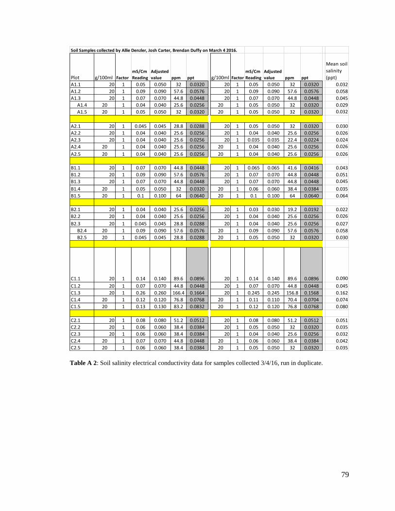
79

Table A 2: Soil salinity electrical conductivity data for samples collected 3/4/16, run in duplicate.

Soil Samples collected by Allie Denzler, Josh Carter, Brendan Duffy on March 4 2016.

Plot g/100ml Factor

mS/Cm

Reading

Adjusted

value ppm ppt g/100ml Factor

mS/Cm

Reading

Adjusted

value ppm ppt

Mean soil

salinity

(ppt)

A1.1 20 1 0.05 0.050 32 0.0320 20 1 0.05 0.050 32 0.0320 0.032

A1.2 20 1 0.09 0.090 57.6 0.0576 20 1 0.09 0.090 57.6 0.0576 0.058

A1.3 20 1 0.07 0.070 44.8 0.0448 20 1 0.07 0.070 44.8 0.0448 0.045

A1.4 20 1 0.04 0.040 25.6 0.0256 20 1 0.05 0.050 32 0.0320 0.029

A1.5 20 1 0.05 0.050 32 0.0320 20 1 0.05 0.050 32 0.0320 0.032

A2.1 20 1 0.045 0.045 28.8 0.0288 20 1 0.05 0.050 32 0.0320 0.030

A2.2 20 1 0.04 0.040 25.6 0.0256 20 1 0.04 0.040 25.6 0.0256 0.026

A2.3 20 1 0.04 0.040 25.6 0.0256 20 1 0.035 0.035 22.4 0.0224 0.024

A2.4 20 1 0.04 0.040 25.6 0.0256 20 1 0.04 0.040 25.6 0.0256 0.026

A2.5 20 1 0.04 0.040 25.6 0.0256 20 1 0.04 0.040 25.6 0.0256 0.026

B1.1 20 1 0.07 0.070 44.8 0.0448 20 1 0.065 0.065 41.6 0.0416 0.043

B1.2 20 1 0.09 0.090 57.6 0.0576 20 1 0.07 0.070 44.8 0.0448 0.051

B1.3 20 1 0.07 0.070 44.8 0.0448 20 1 0.07 0.070 44.8 0.0448 0.045

B1.4 20 1 0.05 0.050 32 0.0320 20 1 0.06 0.060 38.4 0.0384 0.035

B1.5 20 1 0.1 0.100 64 0.0640 20 1 0.1 0.100 64 0.0640 0.064

B2.1 20 1 0.04 0.040 25.6 0.0256 20 1 0.03 0.030 19.2 0.0192 0.022

B2.2 20 1 0.04 0.040 25.6 0.0256 20 1 0.04 0.040 25.6 0.0256 0.026

B2.3 20 1 0.045 0.045 28.8 0.0288 20 1 0.04 0.040 25.6 0.0256 0.027

B2.4 20 1 0.09 0.090 57.6 0.0576 20 1 0.09 0.090 57.6 0.0576 0.058

B2.5 20 1 0.045 0.045 28.8 0.0288 20 1 0.05 0.050 32 0.0320 0.030

C1.1 20 1 0.14 0.140 89.6 0.0896 20 1 0.14 0.140 89.6 0.0896 0.090

C1.2 20 1 0.07 0.070 44.8 0.0448 20 1 0.07 0.070 44.8 0.0448 0.045

C1.3 20 1 0.26 0.260 166.4 0.1664 20 1 0.245 0.245 156.8 0.1568 0.162

C1.4 20 1 0.12 0.120 76.8 0.0768 20 1 0.11 0.110 70.4 0.0704 0.074

C1.5 20 1 0.13 0.130 83.2 0.0832 20 1 0.12 0.120 76.8 0.0768 0.080

C2.1 20 1 0.08 0.080 51.2 0.0512 20 1 0.08 0.080 51.2 0.0512 0.051

C2.2 20 1 0.06 0.060 38.4 0.0384 20 1 0.05 0.050 32 0.0320 0.035

C2.3 20 1 0.06 0.060 38.4 0.0384 20 1 0.04 0.040 25.6 0.0256 0.032

C2.4 20 1 0.07 0.070 44.8 0.0448 20 1 0.06 0.060 38.4 0.0384 0.042

C2.5 20 1 0.06 0.060 38.4 0.0384 20 1 0.05 0.050 32 0.0320 0.035

80

Table A 3: Soil salinity electrical conductivity data for samples collected 2/14/17.

Samples collected by Allie and Conrad on Feb 13-14, 2017

Plot g/100ml Factor

mS/Cm

Reading

Adjusted

value ppm ppt

Avg ppt for

entire plot

A1.5 U 20 1 0.75 0.750 480 0.4800

A1.5 M 20 1 0.97 0.970 620.8 0.6208 0.5589

A1.5 L 20 1 0.9 0.900 576 0.5760

A2.4 U 20 1 1.24 1.240 793.6 0.7936

A2.4 M 20 1 1.35 1.350 864 0.8640 0.7019

A2.4 L 20 1 0.7 0.700 448 0.4480

B1.5 U 20 1 0.77 0.770 492.8 0.4928

B1.5 M 20 1 1.25 1.250 800 0.8000 0.7125

B1.5 L 20 1 1.32 1.320 844.8 0.8448

B2.4 U 20 1 0.88 0.880 563.2 0.5632

B2.4 M 20 1 0.82 0.820 524.8 0.5248 0.5632

B2.4 L 20 1 0.94 0.940 601.6 0.6016

C1.5 U 20 1 1.31 1.310 838.4 0.8384

C1.5 M 20 1 1.16 1.160 742.4 0.7424 0.7360

C1.5 L 20 1 0.98 0.980 627.2 0.6272

C2.2 U 20 1 0.89 0.890 569.6 0.5696

C2.2 M 20 1 1.06 1.060 678.4 0.6784 0.6379

C2.2 L 20 1 1.04 1.040 665.6 0.6656

81

Table A 4: Comparison of soil salinities in unseeded control plots on two dates.

Figure A 1: Graphical comparison of soil salinities in unseeded control plots on two dates.

Control Plot

Mean soil

salinity ppt -

03/04/2016

Mean soil

salinity ppt -

02/14/2017

A1.4 0.03 0.56

A2.4 0.03 0.70

B1.5 0.06 0.71

B2.4 0.06 0.56

C1.5 0.08 0.74

C2.2 0.04 0.64

0.00

0.10

0.20

0.30

0.40

0.50

0.60

0.70

0.80

A1.4 A2.4 B1.5 B2.4 C1.5 C2.2

Mean soil salinityppt - 03/04/2016

Mean soil salinityppt - 02/14/2017

82

Appendix A

Materials

Easy Gardener brand 100% natural burlap fabric. Address: easy gardener products,

inc., p.o. box 21025, Waco, tx 76702-1025

Rainier Fiber™ Premium Wood Fiber Mulch For Hydroseeding and Erosion Control.

Net Wt. 50 lbs/22.7 kg. Manufactured by: Rainier Veneer Inc. P.O. Bos 1250 Graham,

Wash. 98338. 253-846-0242. Date stamp on bag: 07/21-15 15:37.

SPECIFICATION TEST METHOD TEST RESULTS

Moisture content ASTM D 644 12% ± 3%

Organic matter (minimum) ASTM D 586 98%

Ash content (maximum) ASTM D 586 2%

Water holding capacity (minimum) ASTM D 7367 1300%

pH @ 3% fiber concentration SW846 9045 4.5 ± 0.5

Color Observed Green

Mixing instructions

All Rainier products are smooth loading wood fiber mulches with load rates up to 25

bags per 3000 gallons of water or 50 lbs per 120 gallons of water. Loading rates may vary

depending on the type of machine and its working capability.

Mixing instructions:

1) Mechanically agitated hydroseeders:

A. Fill tank with water to bottom of agitator shaft.

B. Start agitation

C. Keep water running while adding fiber until proper amount is reached.

D. Mix slurry approximately 5 minutes for Rainier Fiber. Mix for minimum of 8

minutes for +Tac, BFM, SMM and Supreme to fully activate the additives.

2) Before spraying:

Slow agitator speed down to approximately ¼ speed—just fast enough to keep the

slurry in an active rolling mix. Do not run agitators fast or they will bear air in the

slurry. Slowing down the agitators will help avoid cavitation problems.

83

Appendix B

Contact Information

• Bayshore Preserve

3800 WA-3

Shelton, WA 98584

• Capitol Land Trust

4405 7th Ave SE, Suite 306

Lacey, WA 98503

(360) 943-3012

info@capitollandtrust.org

• Inside Passage Seeds

P.O. Box 639

Port Townsend, WA 98368

1-800-361-9657

(360) 385-6114

forest@insidepassageseeds.com

• Hoyt’s Hydroseeding

Tahuya, WA

360-204-3053

steve@hoytshydroseeding.com

• Mason Conservation District

450 W. Business Park Rd.

Shelton, WA 98584

(360) 427-9436

https://www.masoncd.org/