HYDROSTATIC CURVES

From day to day a ship may be loaded to different drafts and different

trims. Therefore, underwater hull form characteristics over a range of

loading conditions need to be calculated. This is done by calculating

each characteristic at each loading condition (different waterlines).

The results of these calculations are plotted on closely spaced grid

paper. These curves are called hydrostatic curves or curves of form. The

following figure shows such a set. Vertical scale shows the ship’s draft.

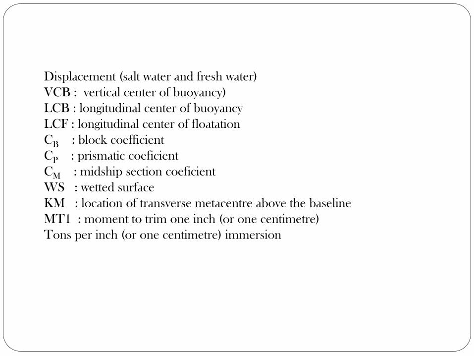
Displacement (salt water and fresh water)

VCB : vertical center of buoyancy)

LCB : longitudinal center of buoyancy

LCF : longitudinal center of floatation

CB : block coefficient

CP : prismatic coeficient

CM : midship section coeficient

WS : wetted surface

KM : location of transverse metacentre above the baseline

MT1 : moment to trim one inch (or one centimetre)

Tons per inch (or one centimetre) immersion

Sample hydrostatic curves

For the convenience of the deck officers , much of the numerical

information shown on the hydrostatic curves is repeated in the form of

tables., which most people find easier to use. In cargo ships this

information is incorporated in the capacity plan, which also shows the

volume of each hold and tank and its centre of gravity. With that

information at hand, the officers can predict the ship’s drafts, fore and

aft and stability characteristics for any proposed condition of loading.

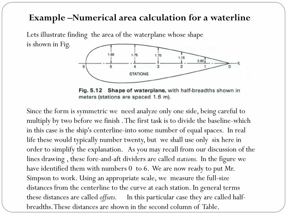
Lets illustrate finding the area of the waterplane whose shape

is shown in Fig.

Since the form is symmetric we need analyze only one side, being careful to

multiply by two before we finish . The first task is to divide the baseline-which

in this case is the ship's centerline-into some number of equal spaces. In real

life these would typically number twenty, but we shall use only six here in

order to simplify the explanation. As you may recall from our discussion of the

lines drawing , these fore-and-aft dividers are called stations. In the figure we

have identified them with numbers 0 to 6. We are now ready to put Mr.

Simpson to work. Using an appropriate scale, we measure the full-size

distances from the centerline to the curve at each station. In general terms

these distances are called offsets. In this particular case they are called half-

breadths.These distances are shown in the second column of Table.

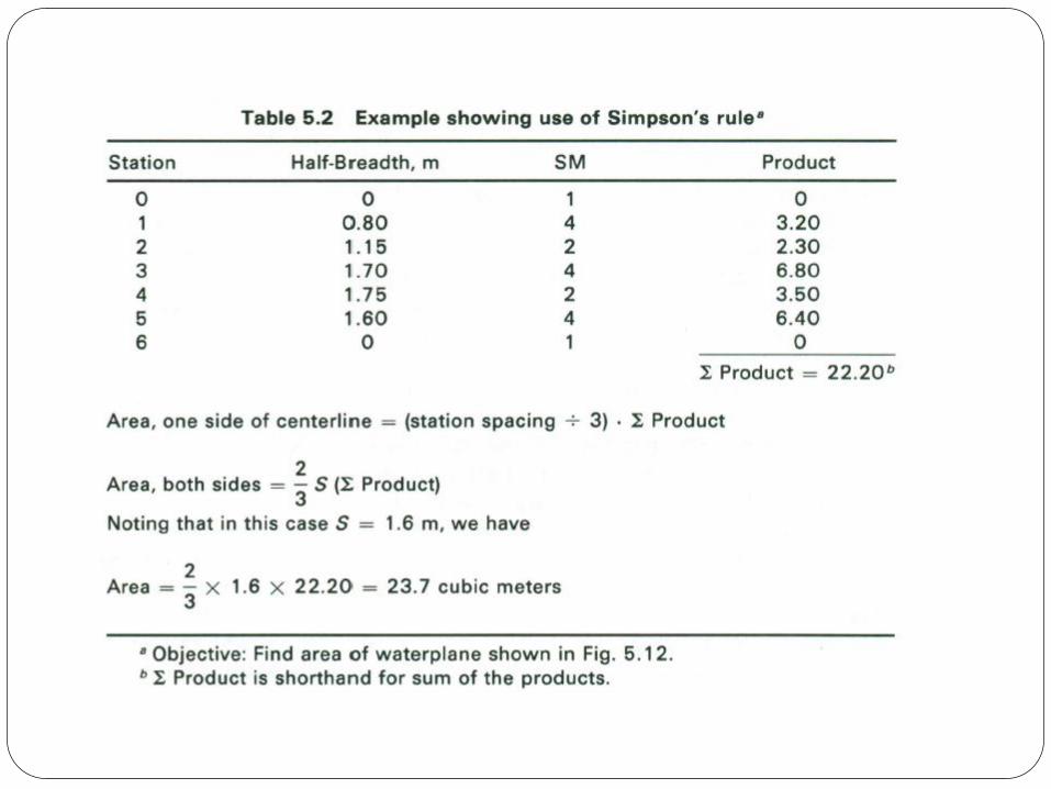
Example –Numerical area calculation for a waterline

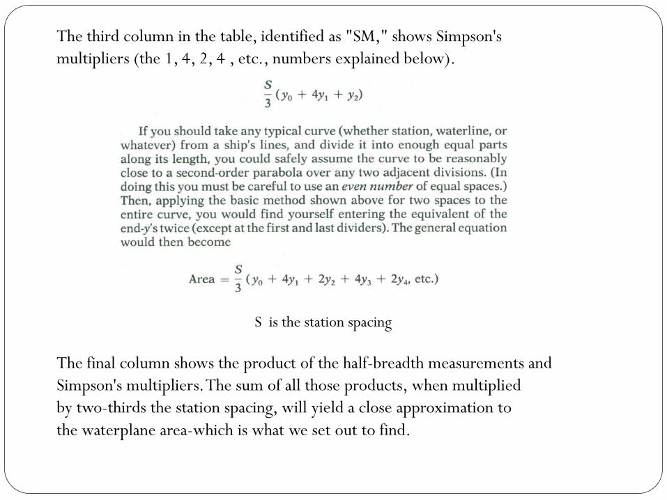
The third column in the table, identified as "SM," shows Simpson's

multipliers (the 1, 4, 2, 4 , etc., numbers explained below).

S is the station spacing

The final column shows the product of the half-breadth measurements and

Simpson's multipliers. The sum of all those products, when multiplied

by two-thirds the station spacing, will yield a close approximation to

the waterplane area-which is what we set out to find.

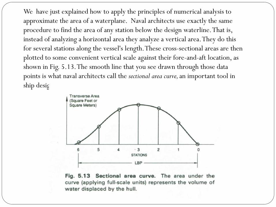
We have just explained how to apply the principles of numerical analysis to

approximate the area of a waterplane. Naval architects use exactly the same

procedure to find the area of any station below the design waterline. That is,

instead of analyzing a horizontal area they analyze a vertical area. They do this

for several stations along the vessel's length. These cross-sectional areas are then

plotted to some convenient vertical scale against their fore-and-aft location, as

shown in Fig. 5.13. The smooth line that you see drawn through those data

points is what naval architects call the sectional area curve, an important tool in

ship design.

In this case we have derived a sectional area curve from a set of lines. If we

now apply Simpson's rule to that curve's offsets, I can derive the ship's volume

of displacement and its longitudinal center of buoyancy. In actual practice, naval

architects often work in the opposite direction.That is, they start by drawing

what they know to be a good sectional area curve and use that to develop the

individual stations, and then fair up the complete lines drawing.This brings up

the question of what is meant by "a good sectional area curve"?

It is one that will provide the required displacement with a longitudinal center

of buoyancy that will lead to minimum wavemaking resistance.

It will also result in acceptable trim fore and aft when the ship is in full-load

condition. In this lesson we have given you an introduction to numerical

analysis in naval architecture.