hydrostatic tensile fracture of a polyurethane elastomer · hydrostatic tensile fracture of a...
TRANSCRIPT

ARL 6-00-UU m I \ I
Aerospace Research Laboratories
HYDROSTATIC TENSILE FRACTURE OF APOLYURETHANE ELASTOMER
GERALD H. LINDSEY
CALIFORNIA INSTITUTE OF TECHNOLOGY
PASADENA, CALIFORNIA
46
CLEAP IM!' 1FOR FEDERAL .I' N. IFIC AND
TEOH~l IT ?." NORATIONTEMI:NIC.&--L i-N, -.,5,•TO
m4.oo -- AL,)L);, --
Distribution of this document is unlimited , "J !
v -
OICOFAEROSPACE RESEARCH "SUnited States Air Force00"
pcý
NOTICES
When overnment drawings, specifications, or other data are used for any purpose other than inconnection with a definitely related Government procurement operation, the United States Governmentthereby incurs no responsibility nor any obligation whatsoever; and the fact that the Government mayhave formulated, furnished, or in any way supplied the said drawings, specifications, or other data, isnot to be regarded by implication or otherwise as in any manner licensing the holder or any otherperson or corporation, or conveying any rights or permission to manufacture, use, or sell any patentedinvention that may in any way be related thereto.
Qualified requesters may obtain copies of this report from the Defense Documentation Center, (DDC),Cameron Station, Alexandria, Virginia.
Distribution of this document is unlimited.
Copies of ARL Technical Documentary Reports should not be returned to Aerospace ResearchLaboratories unless return is required by security considerations, contractual obligations or notices ona specified document.
300 - June 1966 - 773-47-1032
- - -ut.-t ~ -
ARL 66-0029
HYDROSTATIC TENSILE FRACTURE OF APOLYURETHANE ELASTOMER
GERALD H. LINDSEY
CALIFORNIA INSTITUTE OF TECHNOLOGYPASADENA, CALIFORNIA
-i i
FEBRUARY 1966
Contract AF 33(615)-2217Project 7063
AEROSPACE RESEARCH LABORATORIESOFFICE OF AEROSPACE RESEARCH
UNITED STATES AIR FORCEWRIGHT-PATTERSON AIR FORCE BASE, OHIO
S~ii
This is a final report prepared by the Graduate Aeronautical
Laboratories of the California Institute of Technology (GALCIT) for
Aerospace Research Laboratories, Office of Aerospace Research,
t United States Air Force. The work was performed under Contract
No. AF 33(615)-2217, Task 706302-N-3 of Project No. 7063. This
report includes both analytical and experimental results obtained
between 15 October 1964, and 15 November 1965, under the cog-
nizance of the late Mr. Charles A. Davies, ARL Project Scientist.
It is appropriate to acknowledge the help of Mr. William Rae,
lab technician and Marvin Jessey, electronics lab supervisor, for
help in design, preparation and conduction of laboratory experiments.
f• Furthermore, it is a pleasure to express appreciation to Mrs. Sally
Richards and Mrs. Elizabeth Fox, who typed the manuscripts.
The notes and data for this report are recorded in GALCIT
File No. SM 65-25. This report is distributed to the Chemical
Propulsion Mailing List of 1965.
77 >±n-T - 7717
-iii-
ABSTRACT
The investigation of fracture of polymeric materials in
hydrostatic tensile fields constitutes an avenue of approach to the
study of fracture in more general three-dimensional environments.
The advantages created by the symmetry of the stress field are
considerable and, in one of the cases studied, facilitates a theo-
retical treatment that includes large deformations, which are
characteristic of this class of materials.
The analysis is developed through the concept of fracture
originating from a flaw, which in this instance is taken to be a
spherical cavity. Through the application of energy principles,
a theoretical prediction of ultimate strength is made for hydro-
-static tensile fields.
Experiments were conducted to. demonstrate the existence
of such flaws and to evaluate the theory. Results of the tests on
specimens containing both residual flaws and artificially inserted
ones indicate a fundamental difference in behavior as contrasted
with cracks. I
An explanation is given linking experimental results and
theoretical predictions. It is based on the concept that a flaw
"I grows" in the material under load using the cavity as a nucleating
point. Upon this hypothesis is built a theory of rupture in which
planar cracks grow radially from the center of the cavity in the _
Aform of Saturn-ring cracks.
7 "'7 7 7777 Mc
PRIPF-- ~.

S ~-iv-
TABLE OF CONTENTS
PART TITLE PAGE
I INTRODUCTION 1
PROMINENCE OF HYDROSTATIC FIELDS 1
Hydrostatic Tension in Liquids 6
Hydrostatic Tension in Metals 7
Hydrostatic Tension in lrblymers 9
t Related Work 10
Previous Work in Hydrostatic Tension 11
METHOD OF APPROACH 15
Ii THEORETICAL ANALYSIS OF THE POKER- 18CHIP SPECIMEN
4RELATED SOLUTIONS 18
APPFOXIMATE SOLUTION 23
Simplification of the Stress Expression 27
Displacement Expression 31
Limit-Check of the Solution 33
Apparent Modulus 33
End Effect Parameter 34
The Effect of Corner Stress Singularities 36
COMPARISON OF RESULTS WITH OTHER 39SOLUTIONS
Finite Difference 39
Potential Energy Analysis 41
POKER-CHIP SPECIMEN SUBJECTED TO 43COMBINED TRIAXIAL LOADS
Torsion of a Circular Cylinder 44
-'7-
TABLE OF CONTENTS (Cont'd)
PART TITLE PAGE
Stress Analysis of Combined Torsion and 45Extension
Principal Stresses 47
Observations 48
SUMMARY 54
III EXPERIMENTAL ANALYSIS IN HYDROSTATIC 56TENSION
MATERIAL DESCRIPTION 56
Prepolymer Formation 56
Chain Extension 57
Curing or Crosslinking 58
MATERIAL FABRICATION 59
MATERIAL CHARACTERIZATION 63
Bulk Properties 68
Finite Strain Characterization 68
EXPERIMENTAL APPARATUS FOR THE 73POKER-CHIP TEST
Bonding Procedure 75
Ontics 77
Strain Measurements 78
EXPERIMENTAL RESULTS 79 t
Stress-Axis Theorem 82
Description of Fracture 84
Fracture Surface 87
Fracture Propagation 90
-vi-
TABLE OF CONTENTS (Cont'd)
PART TITLE PAGE
"IV FLAW ANALYSIS 93
FLAW DESCRIPTION 93
ENERGY CRITERIA FOR ELASTIC FRACTURE 97
Conservation of Energy 97
Differential Form 98
ENERGY FUNCTIONALS 99
Extended Complementary Energy 100
STABITLITY 101
Buckling Analogy 102
ENERGY FRACTURE ANALYSIS - 104
INFINITESIMAL THEORY
Critical Pressure 105
Flaw Size Dependency 106
Mode of Propagation 107
ENERGY FRACTURE ANALYSIS - EFFECT 107OF FINITE DEFORMATION
Finite Strain Effects 107
CRITICAL FRACTURE POINT 112
Strain Energy 113
Potential of Surface Forces 114
-- Surface Energy 114
CRITICALITY EQUATION 115
Comparative Results 116
V ARTIFICIAL FLAWS 120
OBSERVATIONS 122
9 - 7
I -vii-
TABLE OF CONTENTS (Cont'd)
PART TITLE PAGE
SATURN-RING CRACK 123
Strain Energy Function 125
Criticality Condition 130
Physical Interpretation 132
Limit Cases 136
Numerical Correlation 138
RELATED GEOMETRIES 141
Experimental Results 142
Character of c* 145
SUMMARY 146
VI CONCLUSION 147
REFERENCES 150
1 5
77 I____I
I)
t•
r
CHAPTER I
INTRODUCTION
PROMINENCE OF HYDROSTATIC FIELDS
Hydrostatic tension (HT) and hydrostatic compression (HC)
constitute stress states of a very special class, possessing unique
characteristics of symmetry. Probably the greatest amount of
effort, and certainly the greatest number of results, have come
from investigations with HC, as opposed to HT, where the outstand-
ing work of Bridgman (1.2) has received wide attention. Although
his work has certainly gone well beyond simple HC, he has done
considerable testing directly with it.
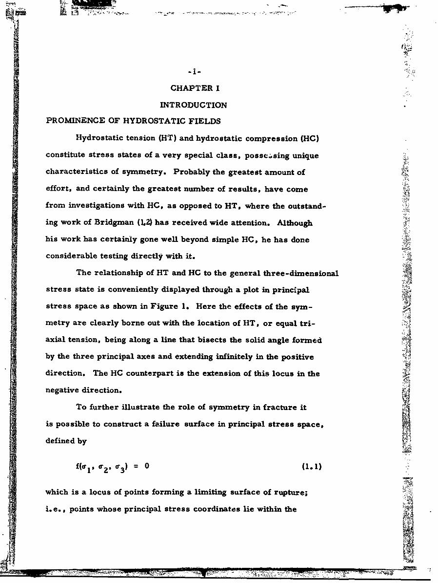
The relationship of HT and HC to the general three-dimensional
stress state is conveniently displayed through a plot in principal
stress space as shown in Figure 1. Here the effects of the sym-
metry are clearly borne out with the location of HT, or equal tri-
axial tension, being along a line that bisects the solid angle formed
by the three principal axes and extending infinitely in the positive
direction. The HC counterpart is the extension of this locus in the
negative direction.
To further illustrate the role of symmetry in fracture it
is possible to construct a failure surface in principal stress space,
defined by
f(cr 1 , o 2 , '3 ) 0 (1.1)
which is a locus of points forming a limiting surface of rupture;
i.e., points whose principal stress coordinates lie within the
77nr

E ---
1'-IV
LI HYDROSTATIC
• ~+0-2
HYDROSTATIC- COMPRESSION
S~+0-1
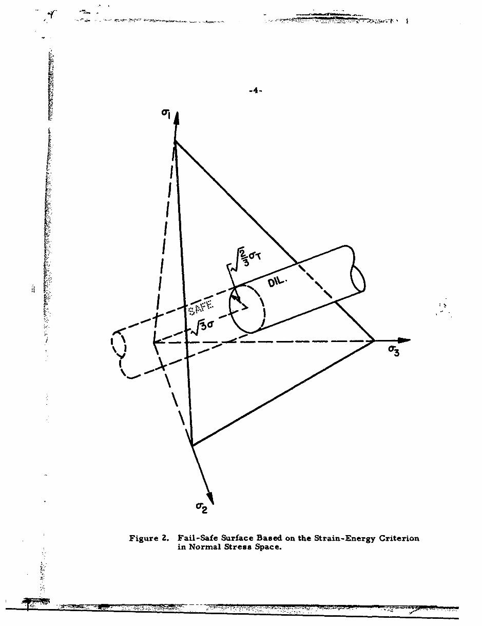
Figure 1. Locus of Hydrostatic Tension and HydrostaticCompression in Principal Stress Space.
I7

-3-
surface will not fail and those lying on or above the surface will
produce failure. Blatz (3) has shown that in general failure, either
from actual rupture or excessive deformation, can be broken down
into a dilatational contribution and a distortional contribution. He
has plotted the pure failure modes of dilatation and distortion in
principal stress space in Figure 2. The stress quality in all octants
may be denoted as follows:
Number ofOctant 0I 02 a3 Positive Stresses
I + + + 3
I + + - 23
m + - + 2
IV+--1
V - + - 2
VI- +-1vlI - - + 1 0•
VII - - - 0
By virtue of equivalence of the three principal axes, it is noted
that there are only four categories of octants characterized by the
number of stresses of the same sign. Thus octants II, MI and V
are similar, and octants IV, VI, and VU are similar. This means
that, for an isotropic material, only four octants need to be tested.
It also means that since the axes of principal stress must be invariant
-4-
ONo
\
I
S~Figure 2. Fail-Safe Surface Based on the Strain-Energy CriterionS~in Normal Stress Space.
r5-1
to the group of rotations in the body, the hydrostatic line becomes an
axis of symmetry and consequently fracture in HT and HC become ex-
tremums; i.e., they are limit points on the failure surface.
Now although there are many obvious similarities between
HT and HC, there is a great deal of difference in the manner in which
materials respond to these two environments fracturewise. The
theory cannot demonstrate that there will be a difference in the actual
configuration of the failure surface; however it has been found
through experiment that there are significant differences. Bridgman
(1) has shown that in combined stress states involving high levels of
hydrostatic pressure, none of the standard failure criteria of maxi-
mum principal stress, maximum principal strain, etc. postulated
from tensile results are accurate. He has investigated many stress
states that cover several of the octants in principal stress space -:
and has found large alterations in the levels of ultimate strains and
ultimate stresses in these other octants when compared to the +++
octant. lie has also discussed (2) the fact that it is necessary before U
rupture can occur to have what he terms an energy release mechanism,
or more simply, a place for the material to go so that energy can be
used to create new surface. Reflection upon this point leads to the k
conclusion that in pure hydrostatic compression fracture could never
occur and the ultimate strength would be infinite. However, slight
perturbations from this field would provide enough anti-symmetry
to allow fracture to occur at realistic levels. Therefore in hydro- IT
static compression the failure surface possesses a cusp at infinity,
which would be in strong contrast to the same situation in tension
woo N Uv~_~~7,, -7 74A~>-7-7 -.--
N -6-
where there is an energy release mechanism, and fracture can occur
at finite values. It then follows that HT and HC produce quite a dif-
ferent effect upon materials, and the resulting behavior in each case
is not the inverse of the other.
One additional point that needs further emphasis is the mathe-
-matical simplicity that arises as a consequence of the symmetry in
the problem. The number of existing solutions to three-dimensional
elasticity problems is limited, but in this instance the theoretical
analysis accompanying the experiment is not only possible but reason-
ably simple, even in the case of finite deformation theory. (4) It makes
a solution possible where it otherwise may be intractable. All of
these factors combine to make HT and HC fields of considerable
interest, as well as of considerable value.
Hydrostatic Tension in Liquids
Although HC lends itself well to experimentation, states of HT
are not so readily generated in the laboratory. One exception to this
is in the case of liquids where HT can readily be created, and as a
consequence, fracture of several liquids has been investigated. (5)
Studies of this type not only contribute to the fundamental knowledge
of physics, but are )f considerable engineering interest as they relate
to the phenomena of cavitation. Fisher (6) has applied an energy
balance to the growth of a spherical cavity in a liquid, and from this
has been able to derive an expression defining the critical pressure
at which the bubble will grow.
-7-iI P - z_ Pv(1.2)
c r P"
where Pc = critical pressure
i y = surface tension
r = radius of cavity
Pv = vapor pressure (usually neglected)
Irwin (7) has extended the analysis of Fisher and favorably compared
his theory with data on the fracture of liquids obtained from several
other investigators. A large number of experimental uncertainties,
very difficult to control, made the correlation somewhat fortuitous,
and thus led Irwin to conclude that the theoretical strength calcula-
tions for pure liquids were of doubtful practical utility. Nevertheless,
as he states, the degree of completeness permitted in the theoretical
considerations, primarily due to the symmetry involved, make the
pure liquid tensile strength analysis of importance. Furthermore,
it can act as a limit case for the more general viscoelastic material,
which we will refer to in a later chapter.
Hydrostatic Tension in Metals
Fracture studies for general combined stress states have been
pursued for metals quite arduously. (8) With complex testing equip-
ment capable of applying fluid pressure as well as tensile shear and
bending loads, it has been possible to study metallic fracture under
a wide range of loading conditions, but not HT. Nadai (9) has traced
some of the attempts to create HT in metals. Two of the methods
employed, which are of a similar nature, are thermal stresses and

S~-8-
"grain transformations. Here attempts are made to produce a state
Sin the body such that one portion pulls on another portion , putting it
in HT,. either by thermal gradient or by volume change due to phase
transformation. Although some success has been realized in pro-
j2 ducing the desired condition, it has never been possible to obtain
any quantitative measurements from such tests. Another popular
method has been the use of a circumferential notch on a circular
cylindrical bar. It was believed that the stress state at the base of
a sharp hyperbolic notch was hydrostatic when the bar was under
axiad tension. However, Neuber (10) in his treatise on notch stresses
demonstrated that this was not the case and that near the surface of
the notch the stress ratios were actually 1:1:3, with the largest being
in the axial direction. Unfortunately the test has not been useful for
other combined tensile stress states in the +++ octant due to the
large gradients of stress in the neighborhood of the notch, which is
the region of interest. Still another attemrpt was made by Lehrer
and Schwalzbart (11) as they bonded a thin sheet of brass between
two plates of steel and pulled the plates in tension perpendicular to
the large, flat face. This test has promise but primarily for mater-
ials that are nearly incompressible. This will be demonstrated in
a later analysis.
So in metals it still remains to find a good hydrostatic tensile
test; although almost any other combination of stress can be imposed.
It is interesting that in spite of this missing piece of information
McAdam, (12) from other experiments, postulated that HT would be
an extremum point on a convex fracture surface; i.e., this stress
. .4

state would represent the maximum in ultimate strength that could be
enjoyed by a brittle metal in tension. It is also interesting to note
that this has subsequently turned out to be the case in other engineer-
ing materials, such as polymers, where it is possible to produce HT
in the laboratory.
Hydrostatic Tension in Polymers
Polymeric materials are fundamentally different in their basic
structure and in their behavior. (13,14,15) Their difference is so
pronounced that special methods of stress analysis, upon which frac-
ture analysis is built, have had to be developed. The state of this
art has recently been reviewed by Williams. (16) Differenceri in the
basic structure produce differences in their fracture behavior, which
has been reviewed first by Bueche and Berry, (17) and subsequently
by Williams. (18) Widespread interest in the fracture properties of
these materials has arisen through a vastly expanding usage of poly-
mers in engineering applications where structural integrity is an
item of concern. One primary example, which attracts the interest
of Aeronautical Engineers, is the structural integrity of solid pro-
pellant rocket grains. (19) In this instance, the solid propellant fuel
constitutes an integral part of the structure; thereby requiring analy-
sis of its material integrity like any other structural component.
However, the constitution of these materials is very complex. It
consists of a binder material, which is an amorphous elastomer,
impregnated with a high volume percentage of solid oxidizer parti-
cles such as ammonium perchlorate. This system is neither
71_ !4
- - -
-10-
homogeneous nor isotropic, and it is innately very complicated in its
mecl~anical behavior. It therefore is reasonable to seek a simplified
approach to the problem with the aim of discovering some of the
fundamentals of the behavior of the separate components; i.e., to
investigate the fracture properties of the amorphous rubber binder
as a first approach to an investigation of the filled system. An
examination of fracture in amorphous rubber also has its own in-
herent interest as it would apply to other engineering applications
where there is no filler involved; thus the incentive for the investiga-
tion of fracture is two-fold: (i) the attempt to study failure in solid
propellant materials for their own sake, and (ii) to discover general
principles that can be applied directly to the fracture analysis of
engineering components where the amorphous polymer alone is the
structural material.
Related Work. In order to place the HT work in proper
perspective, reference will be made to related work in other stress
states. Most of the effort expended on unfilled elastomers has thus
far been applied to the case of uniaxial tension. Certainly this is the
logical starting point, for it keeps complication to a minimum, so
that experimental results are uot obscured by extraneous influences.
However, even in this simple case much work has been required to
uncover and define basic behavior in terms of mechanical properties.
A comprehensive review of the uniaxial work has currently been
given by Landel and Fedors, (20) which devotes some attention to
the elusive problem of fracture properties under general loading
~ _ 5r. ,12

] ~-11 -
conditions. This is the area in which there is still much to be done
even in the uniaxial state, for the concepts of fatigue and cumulative
damage are not only unsettled, but investigations are still in their
infancy even though preliminary information is now coming forth as
evidenced by the work of Knauss and Betz. (21)
Concurrently there has been a similar, but smaller, corps 4:
of investigators working with multiaxial polymer fracture. Two
biaxial tests have been used, one referred to as the strip biaxial
which has probably received the most attention is shown in Figure 3
and the other is that of the equal biaxial test, which can be conducted
by inflating a membrane (Figure 4) or in some instances special
fixtures have been successful. (See Ko (22).) These tests are quite
tedious. Furthermore it is difficult to force fracture to occur away
from the grips, and they require considerable care in the prepara-
tion of the specimen to yield a cross-section that will produce the
desired stress. field; consequently a limited amount of results is
available for these geometries. One extensive work using several
stress fields in uniaxial, biaxial, and triaxial tension to construct
IIfailure surfaces has been completed by Ko. (22)
Previous Work in Hydrostatic Tension. There has been even
less work done in the area of triaxial fracture. One of the first
efforts in this direction was made by Gent and Lindley, (23,24) who
performed tests in HT and HC. They were attracted to an unusual
test by which they produced these fields following work reported by
Yerzley (25) on the bond integrity between rubbery materials. Ina,.
IN
*1 -
1 -12-
I:
Fiue3 ti-BailTnin
................................... -

PSOLITHANE 113 ("
0 77
SOLITHANE 113SHEET- (INFLATED)
Figure 4. Equal Biaxial Membrane Test.
'-7 - ~'-'- ---~ - - - - '.-~ --- 4---"goo

-14-
Yerzley's search for an ASTM standard, he glued a single thin rec-
tangular block of rubber between two similar metal blocks and pulled
them apart to test the strength of the interface bonds. In the course
of the experiments, he noted a rather peculiar type of fracture in the
rubbery specimen and discussed it briefly. Twenty years later Gent
and Lindley pursued this test by manufacturing some small circular
disks from a carbon black filled, natural rubber and pulled them by
means of two, rigid, steel plates. With the thin disk of soft specimen
material glued and sandwiched between the stiffer grips, it will be
restrained from contracting laterally as the entire assembly is ex-
tended along its axis perpendicular to the face of the disk. This
creates the triaxial stress field. The amount of restraint is a func-
tion of the aspect ratio (diameter to thickness) of the specimen, but
an elementary analysis can be made by assuming the disk to be
infinitely thin such that the external radius is sufficiently far from
the center to assume that the only non-zero displacement, w, is in
the x 3 direction. With this configuration the boundary conditions
become u v = 0 from which Er = FE = 0. The stress field then
becomes
or a •e0= -z (1.3)
where use has been made of the axial strain
az- (1-2v)(l+v)'=1 - v) (1.4)
so that the apparent axial modulus becomes
so $V
* ~ Y.sq~ .~- -~ *. -
-AE .5
S(.1-5V
where it may be noted that for rubbery materials which are charac-
teristically incompressible, i.e., v = 1/2, the triaxial tensile stress
state approaches hydrostatic with the consequent infinite apparent
axial stiffness. Gent and Lindley's initial experimental work demon-
"strated an internal fracture in the rubber which varied with thickness,
modulus and tensile strength, and they devoted their attention to
documenting and explaining this variation. After completing a pre-
liminary probe into this interesting mode of fracture, they extended
their work to compression using carbon black filled rubber specimens.
Emphasis was placed on defining the load-deflection relation and
obtaining a definition of the stress field in the specimen.
METHOD OF APPROACH
The work of Gent and Lindley will be used as a point of de-
parture for the work to be reported. The first item to receive
attention will be a detailed stress analysis of the test specimen to
provide a means of local examination of the experimental results.
This will be coupled with experimental work made on a modified test
apparatus, which permits a more detailed study of the fracture pro-
cess. Interpretation of these results and analytical extensions
thereof will then be made on the basis of a flaw hypothesis. A word
of justification for this assumption is in order.
Many analytical and experimental techniques currently
applied to polymers were carried over from metal fracture.
lg
*
-- -6
Although several have been found to apply directly, as yet no univer-
sal approach has been discovered. However, in specific instances,
particular approaches have been fruitful. For instance, through
laboratory experience it has been found that many polymers are very
notch sensitive; i.e., their properties are strongly controlled by
imperfections on the surface as well as in the interior of the body.
Such behavior suggests that an investigation'of the fracture phenom-
enon in these materiala may appropriately be made by means of a
flaw hypothesis. This method can be employed on either the molecu-
lar or the continuum level. Physical chemists have studied the
effects of flaws in the chain structure itself, and worked up by
statistical means, through groups of chains, to the continuous
specimen, where correlations can be made between specimen load
and localized stress at the molecular flaw. A consideration of the
bond energies then leads to a prediction of fracture. Early ideas
of this type we-e put forth by Houwink (26) and later expanded by
investigators such as Flory, (27) who was an advocate of molecular
flaws due to dangling chain ends. Currently this approach is yield-
ing results due to improved mathematical techniques, including the
recent work of Blatz (28) and Knauss (29).
An alternate approach is to consider the material initially
as a continuum and then represent the flaws as discontinuities in
that continuum. Through an analysis of a typical flaw, which in one
instance is a spherical cavity taken to be independent of all other
flaws in the material, the local conditions of stress, strain, and
energy, can be computed and fracture predicted through the
application of an energy criterion. (30) This will be done for two
different modes of propagation of the fracture surface, and subse-
quentl) a comparison of the two leads to new insight into the behavior
of holes and cavities. One further point should be noted before pro-
ceeding. Amorphous elastomers characteristically are viscoelastic
(31) and exhibit large deformations in fracture. (32) These charac-
teristics complicate the analysis considerably, especially as the
theory of finite viscoelasticity has not yet progressed to the point
that it is a practical tool for analysis. For this reason the work
referred to hereinas well as this entire effortis predominantly
performed with the classical tools of infinitesimal elasticity (and
in some cases infinitesimal viscoelasticity) and should be inter-
preted as an exploration of the broad concepts of polymeric fracture
in HT rather than a final definitive treatise of the subject.
*f
Schapery (33) has just completed a report that promises to helprectify this situation and make finite viscoelasticity a bit moremanageable for engineering analysis.
-V
-18-
CHAPTER II
THEORETICAL ANALYSIS OF THE POKER-CHIP SPECIMEN
The mathematical model of the poker-chip configuration,
shown in Figure 5, leads to a mixed boundary value problem that
is almost analytically intractable from the standpoint of classical
elastic theory. Like many elastic problems involving finite bodies
with discontinuous boundary conditions, the poker-chip configuration
presents many mathematit al difficulties if an exact, closed-form
solution is sought. However, for such problems series solutions
are possible and several have been used.
$1 RELATED SOLUTIONS
One of the first theoretical analyses relating to this problem
was published by Pickett. (34) In his analysis of cylirders, he
* employed a Fourier series expansion, which resulted in the final
solution being expressed in terms of a doubly infinite series.
This form is awkward for our purpose, where the results are in-
volved in a subsequent analysis of fracture, especially where
convergence of the solution is slow. This is emphasized near the
corners, where it should be noted that the problem of convergence
is basic due to the peculiar geometrical effects present there.
There is a discontinuity in material, as wel as discontinuities
from stress to displacement boundary conditions, and this may
lead to mathematically infinite stresses. (35) When the stress
singularity does occur, and such singular behavior has not been
explicitly built into the form of the formal representation of the

-19-W
~ PPLIED LOAD
r. u
Figure 5. Tria~da1 "Poker-Chip" Test and the CoordinateSystem Used in the Stress Analysis.
4 1 I I -- -
-20-
"solution, convergence and rate of convergence difficulties are to be
expected.
Gent and Lindley (23) began by solving an analogous problem
of an infinite slab, using intuitive assumptions based on incompres-
sible material behavior and proposed a stress analysis, which can
be shown equivalent to minimizing the potential energy. They then
extended this line of reasoning to the circular disk, and the apparent
modulus deduced from this analysis was compared to a large amount
of experimental data. Qualitatively there was good agreement, al-
though quantitative predictions with the theory were good only for a
very small range of aspect ratios. Furthermore, since the apparent
'S modulus is essentially an average property, the corresponding
internal stresses needed for failure analysis could be significantly
different than the average value.
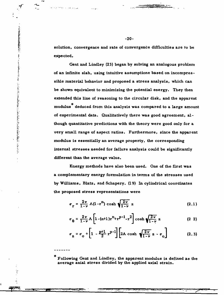
Energy methods have also been used. One of the first was
a complementary energy formulation in terms of the stresses used
by Williams, Blatz, and Schapery. (19) In cylindrical coordinates
the proposed stress representations were
a-=2v A(I-r n) cosh J2 v
r= z (2.1)
a' =!A [1-(n+l)rn+rP-l-r2] cosh -I~z (2 2)
W fo+[1 21!-rP-1][2Acosh .Z- o] (2.3)
Following Gent and Lindley, the apparent modulus is defined as the
average axial stress divided by the applied axial strain.
-21-
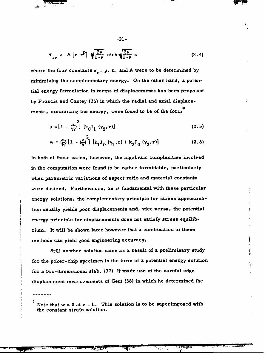
"rz= -A [r-rp] •i sinh 1 - z (2.4)
where the four constants o0, p, n, and A were to be determined by
minimizing the complementary energy. On the other hand, a poten-
tial energy formulation in terms of displacements has been proposed
by Francis and Cantey (36) in which the radial and axial displace-
ments, minimizing the energy, were found to be of the form*
2u - (I) ] [koJ 1 (J 2 ,r)] (2.5)
2w =()[I - () I [kJJ0 (Ylr) + Jo(Y2 .r)] (2.6)
In both of these cases, however, the algebraic complexities involved
in the computation were found to be rather formidable, particularly
when parametric variations of aspect ratio and material constants
were desired. Furthermore, as is fundamental with these particular
energy solutions, the complementary principle for stress approxima-
tion usually yields poor displacements and, vice versa, the potential
energy principle for displacements does not satisfy stress equilib-
rium. It will be shown later however that a combination of these
methods can yield good engineering accuracy.
Still another solution came as a result of a preliminary study
for the poker-chip specimen in the form of a potential energy solution
for a two-dimensional slab. (37) It made use of the careful edge
displacement measu-ements of Gent (38) in which he determined the
Note that w = 0 at z = h. This solution is to be superimposed withthe constant strain solution.
-- /I 1

49)
transverse displacements to be mainly parabolic functions of thep longitudinal (axial) coordinate. Results of the slab analysis furnished
an increased understanding of the complete stress distribution,
including the extent of the boundary influence on the internal stresses
and the fact that the axial displacement of the slab was virtually
constant throughout. Building upon this foundation it was possible
to compute two approximate solutions for the disk. The first in-
volves a technique of averaging the stresses through the thickness
of the specimen and satisfying the equilibrium equations on an
average basis. The other employs the variational approach for
the minimization of the potential energy. Both use assumed func-
tional forms for the displacements, which are guided by the slab
analysisi and the two methods bear a strong similarity throughout.
This will be demonstrated in detail later as both solutions are dis-
cussed.
Finally, numerical solutions to the problem have been
obtained by Messner, (39) and Brisbane. (40) In Messner's solu-
tion, for instance, a finite difference technique has been used,
and the grid size has been progressively reduced until two sub-
sequent sizes produce no appreciable change in the stress state.
The calculated stress distribution wili be presented graphically
later to act on a basis of comparison for the accuracy of the ap-
proximate analytical solution. The convergence at the corners
has been found to be extremely slow, and this is again due to the
presence of stress singularities at these points. This type of
computer program offers great practical advantages, since a
R 4i I •_ T 71•
-23-
solution can be obtained to any desired accuracy in a short time.
However it has the disadvantage that in order to perform a para-
metric study, a separate calculation has to be performed for each
configuration.
APPROXIMATE SOLUTION
This section describes an approximate method for analyzing
a thin, circular disk developed by Lindsey, Schapery, Williams
and Zak. (41) As mentioned previously it uses an extension of the
solution fnr a slab in plane strain. (37) One of the primary advan-
tages of this solution is that the incompressibility assumption
made by Gent and Lindley (23) does not have to be invoked so that
the resulting solution is applicable over a range of material prop-
erties. Figure 5 shows a circular disk of radius a with its axis
in the z-direction, and the faces z = 11 bonded to rigid plates. We
assume that the disk is loaded by increasing the thickness by 2E
and proceed to select two displacement functions, which satisfy
the boundary conditions on that part of the boundary where dis-
placements are prescribed. Note that the third (circumferential'
displacement, v, is identically zero by reasons of symmetry.
Such functions would also be admissible functions for use in the
Theorem of Minimum Potential Energy, although it should be
recalled that the resultant minimization yields a result, in this
case it will turn out to be the function g(r), such that the equations
of equilibrium are not satisfied unless the solution is actually
exact. The radial displacement function is known to be ezaentially
4 -24-
parabolic from the edge measuiements by Gent. (38) The longitudinal
displacement was found by Schapery and Williams (37) to be directly
proportional to its distance from the horizontal plane of symmetry
over most of the disk. Consequently the displacement functions take
the form
U -(l-z 2 )g(r) (2.7a)
w =6 z (2.7b)
in the radial and thickness directions respectively. Note that the dis-
placement boundary conditions are satisfied at the surfaces z = A1,
and that g(r) is presently an unprescribed function of the radius. The
strains corresponding to these displacements are easily found to be
=r aur g'(1-z2) (2.8a)
= .1- -= (I-z 2 (2.8b)e r r8w
Fz = aw =_ E(2.8c)
8u &"Wrz z r (2.8d)
from which the z-averaged stresses are found as
1
72'd ( 9 1& (2. 9a)-1
1
0 To" (3 r- (Z. 9b)
-1
-1
ft- 9• + •I~ ( •2 . _c

-25-
'Trz = Zgz (2.9d)
where g' dg/dr.
The function g is found from the condition that the z-integrated
equilibrium equation for the radial direction is to vanish, i. e.,
.Z OT rz + dz = 0 (2. l Oa)
or
r + T + 0 (2. 1Ob)dr rz z=1l r
Also, note that because of symmetry the integrated equilibrium equa-
tion for the z-direction is satisfied identically,
10r0- 1~~~~ rzJ zO(.1ýrz + -Wz +-r dz = 0 .ll
-1
Substitution of stresses (2. 9) into equation (2. 10) yields the
differential equation for g, thus
g,,~ +g _;L + M)g= 0 .l)
where M is a constant made up of a composite of material properties.
= 3 0-Z0 (2.13)X+211 i 717-V7
Equation (2, 13) is a form of Bessel's Equation and yields modified
Bessel functions as solutions.
-26-
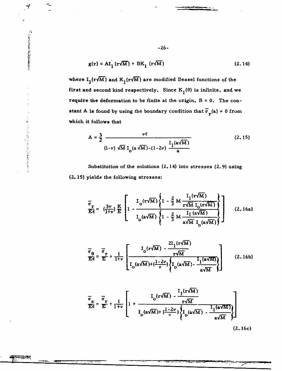
g(r) = AII (rN"') + BK1 (rvr") (2.14)
whereI Il(r-A=1) and Kl(r4M$) are modified Bessel functions of the
first and second kind respectively. Since KI(0) is infinite, and we
require the deformation to be finite at the origin, B = 0. The con-
stant A is found by using the boundary condition that r (a) = 0 from
which it follows that
I1 (a1 =)12.15):_ ~I1 (a4-M"
(l-v) I'M Ioav')-ll-Zv) a
Substitution of the solutions (2. 14) into stresses (2.9) using
(2. 15) yields the following stresses:
Io(r -IM) I - -M r- or
fr 3v K [ { 3 rV ?Ioir7¶Mj (2.16a)"(OY "- { 11(,[-[ I°(aV"M') ~1 -4- M ae oarMM
L 3 -1 (r -K - 1)
•'r 1 0 ( r rM -) 2 1 i (r4 M(
. b
TO r ÷+ [ II) (Z. 16b)
M -oI (a - )+ (I -) I O(a,) - af'M
(2. 16c)
-- .1 0 (r 4M- -
z r +m + • • M •• •
(r--3v), v'i ___ z (2. 16d)
<lM I~aM
which, it may be found, approaches a state of triaxial, hydrostatic
tension at the center in the case of an incompressible material. We
expect the stresses (2. 16) to be good approximations for 0 •< v •< 1/2
except for the singular stresses near the free-edge r =a.
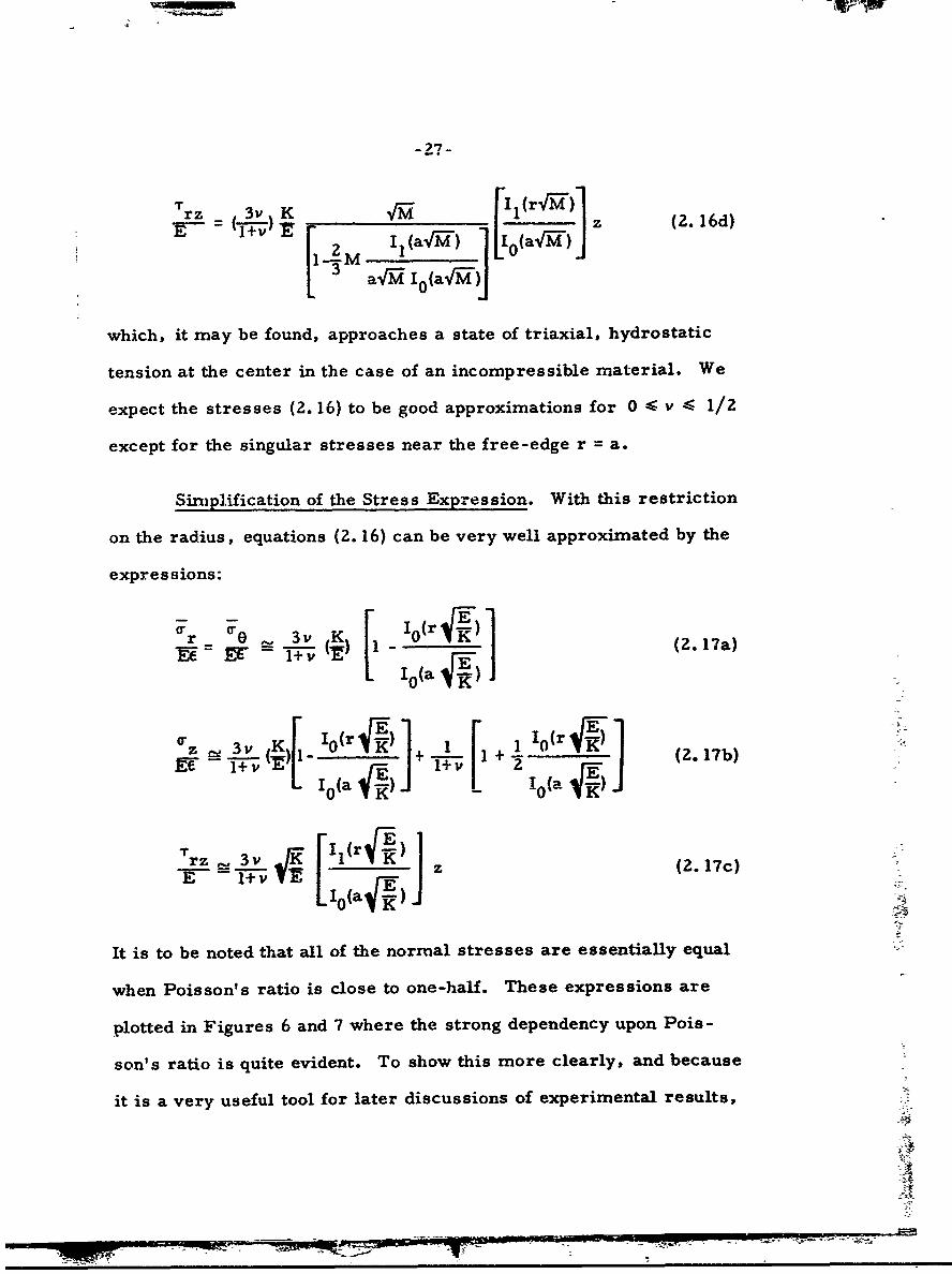
Simlplification of the Stress Expression. With this restriction
on the radius, equations (2. 16) can be very well approximated by the
expre ssions:
O]9=%,' 3 K • --(4•) (2. 17a)
loI~(a-
. _= , z (2. lic) '
lola ) ,
It is to be noted that all of the normal stresses are essentially equal
when Poisson's ratio is close to one-half. These expressions are
plotted in Figures 6 and 7 where the strong dependency upon Pois -
son's ratio is quite evident. To show this more clearly, and because
it is a very useful tool for later discussions of experimental results, ,

120
100V-0.49995
E6 60-
40-
20
-): 0.4737
0.11
0 0.2 0.4 0.6 0.8 1.0a
Figure 6. s-Nortnal Stress in Disk vs6rl/2 20-ZO
12
10
V= 0.49995
8F
V -0.4995
Ee
=0.4975
2= 0.4737
\7=0.4118
0 0.2 0.4 0.6 0.8 1.0
ra
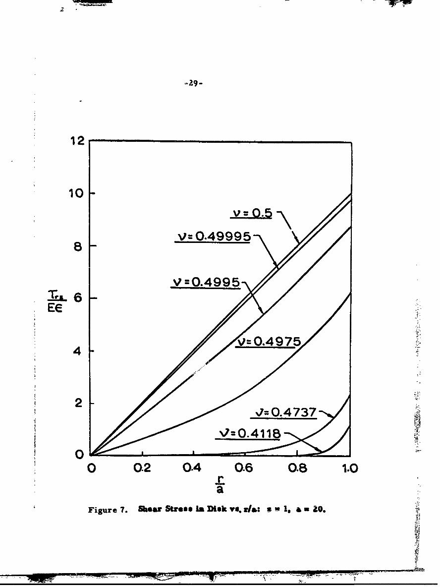
Figure 7. Shear Stiess ln Disk Va. cla: n 1. 0. .41
-'-~-~--.--~--~-'-' V
-30-
t 100
80
~J~60
40
200.4960 0.4980 0.5000
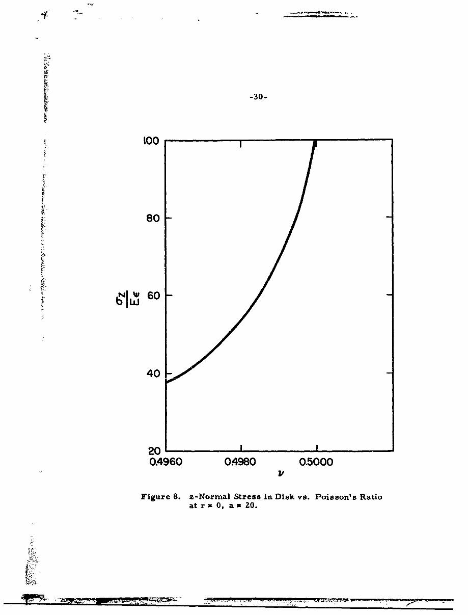
Figure 8. z-Normal Stress in Disk vs. Poisson's Ratioat r x 0, a x 20.
+R
-3'-
a cross-plot of Figure 6 is given in Figure 8, where the relationship
of local stress to applied strain is shown for r = 0.
Strictly speaking the only point of true HT is at the midplane
z = 0; however as seen in Figure 7 the shear stress at the rigid
boundary, which is the region of maximum shear, is only a small
percentage of the normal stresses. Consequently for all practical
purposes the stress field can be considered HT as far out as r = 0. 5a
with very little error. Furthermore for materials with Poisson's
Ratio down to 0. 4975 or below, there is an appreciable central region
of virtually constant hydrostatic stress, which contributes to the ease
and accuracy with which data can be reduced. Large stress gra-
dients make it difficult to know with precision what the local fracture
levels actually are.
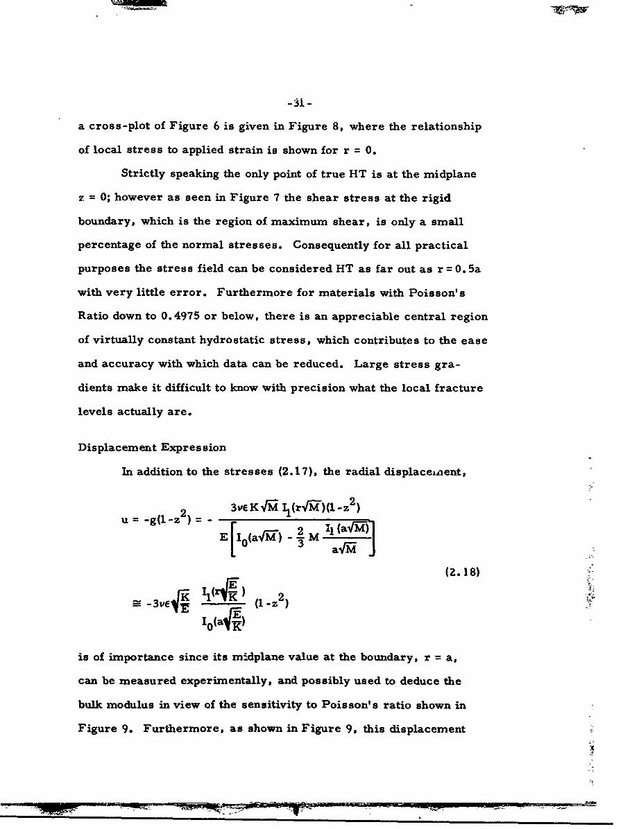
Displacement Expression
In addition to the stresses (2.17), the radial displaceinent,
2 3ve K -IM-I(rVri?)(1-z2 )
u -g(1-Z , a I
(Z.18)
--v r (1-Z 2
-I(a E~
is of importance since its midplane value at the boundary, r = a,
can be measured experimentally, and possibly used to deduce the
bulk modulus in view of the sensitivity to Poisson's ratio shown in
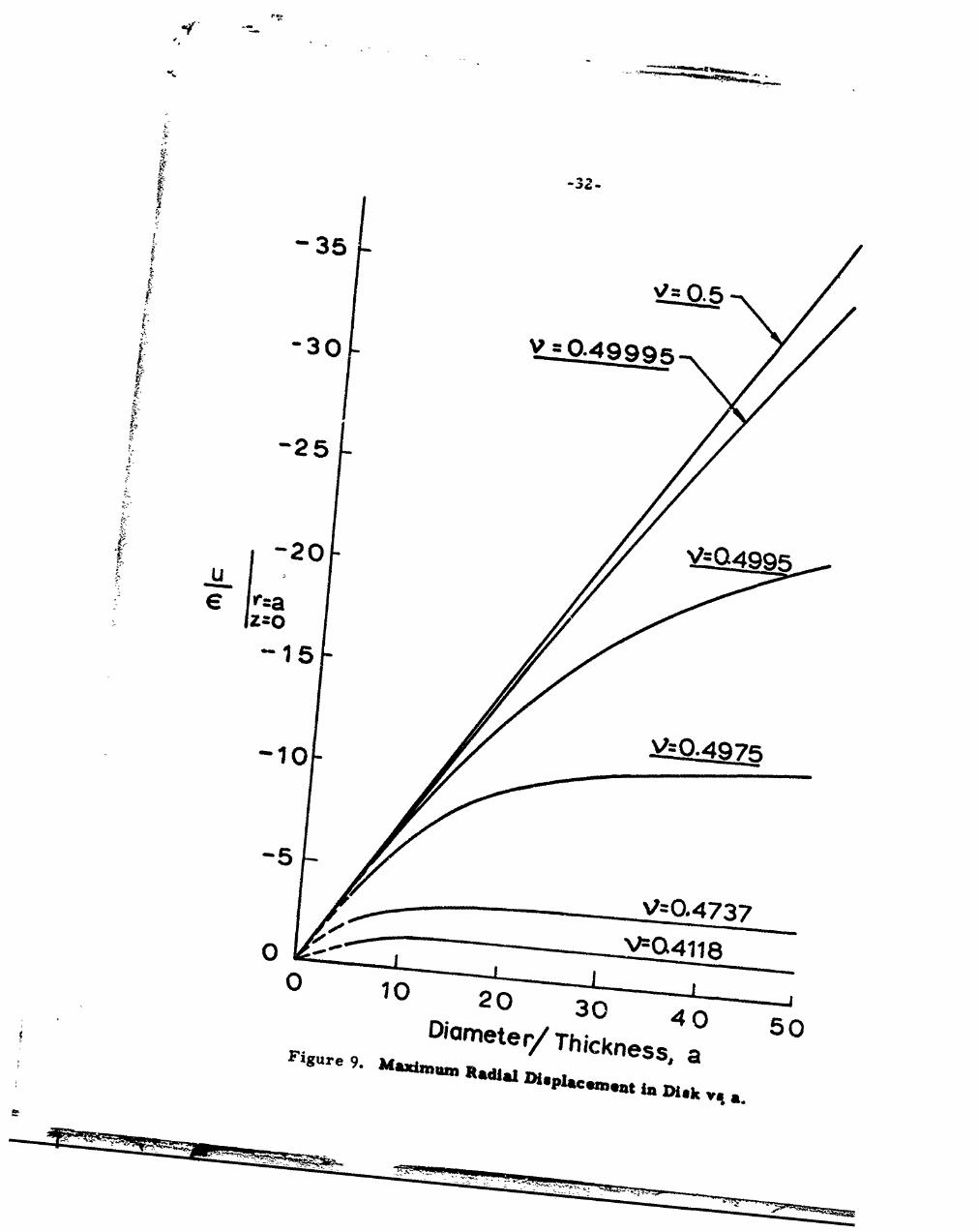
Figure 9. Furthermore, as shown in Figure 9, this displacement"A'
•a ' WNmm m
IC
4.35
"-30 V0.49995
M25
10
Figure Dimeer ThiCknesS. aRadial JDisplaComen iA Disk v t a.
-33-
may be very large for nearly incompressible materials, even when
the nominal strain, e, is small. In the neighborhood of the radii for
which the radial displacement is not small relative to the disk thick-
nesses, some error due to large strains will be introduced in the
results of the present linear analysis.
Limit-Check of the Solution
In the incompressible limit case (v = 1/2) solutions are
readily found from equations (2.16) and (2.18) to be
yr. =9 1 2r = (a2_-r 2 (2.1 9a)
- 1 (a2-r2) + 2 (2.19b)
rz rz (2.19c)
where it may be noted that for a large aspect ratio, the condition
(r = 0) of triaxial hydrostatic tension is achieved. Further,
3 2uu - Err ( ) (2.19d)
Apparent Modulus
Another quantity of experimental interest is the apparent
i uniaxial modulus EA, defined as the ratio of the average stress
over the bonded surface ca- required to produce the axial dis-
placement w, to the nominal axial strain 6, viz.
ZA 24 ar-azrdrE = = 0 2 (2.20)
AA ra
7;T
-34-
Upon substitution of a-, equation (2.16c), into (2.20) we find
E 2J 2(alfi)A~ 3v K _ _ _ _
- v ) "aa i 0 (a -lM-)
(2.21)"-I, (a-'rM
++� 2 k (aVM) 1 +12._. 0 (i" ]S" aV Io (aVM
This apparent modulus can be conveniently employed for
determining the bulk modulus of nearly incompressible materials.
Namely, given an aspect ratio a, and experimentally measured
modulus EA# the modulus ratio E/K can be deduced from a graph
of equation (2.21), such as shown in Figure 10. It is observed
that EA/Ea 2 depends on only the parameter a"'E-IK for a ' 30.
The accuracy of expression (2.21) is expected to be good, even
for small aspect ratios. This follows from the fact that the appar-
ent modulus is an average property, and therefore should not be
sensitive to error in stress near the periphery. Furthermore,
EA has the correct limiting value of E for a = 0.
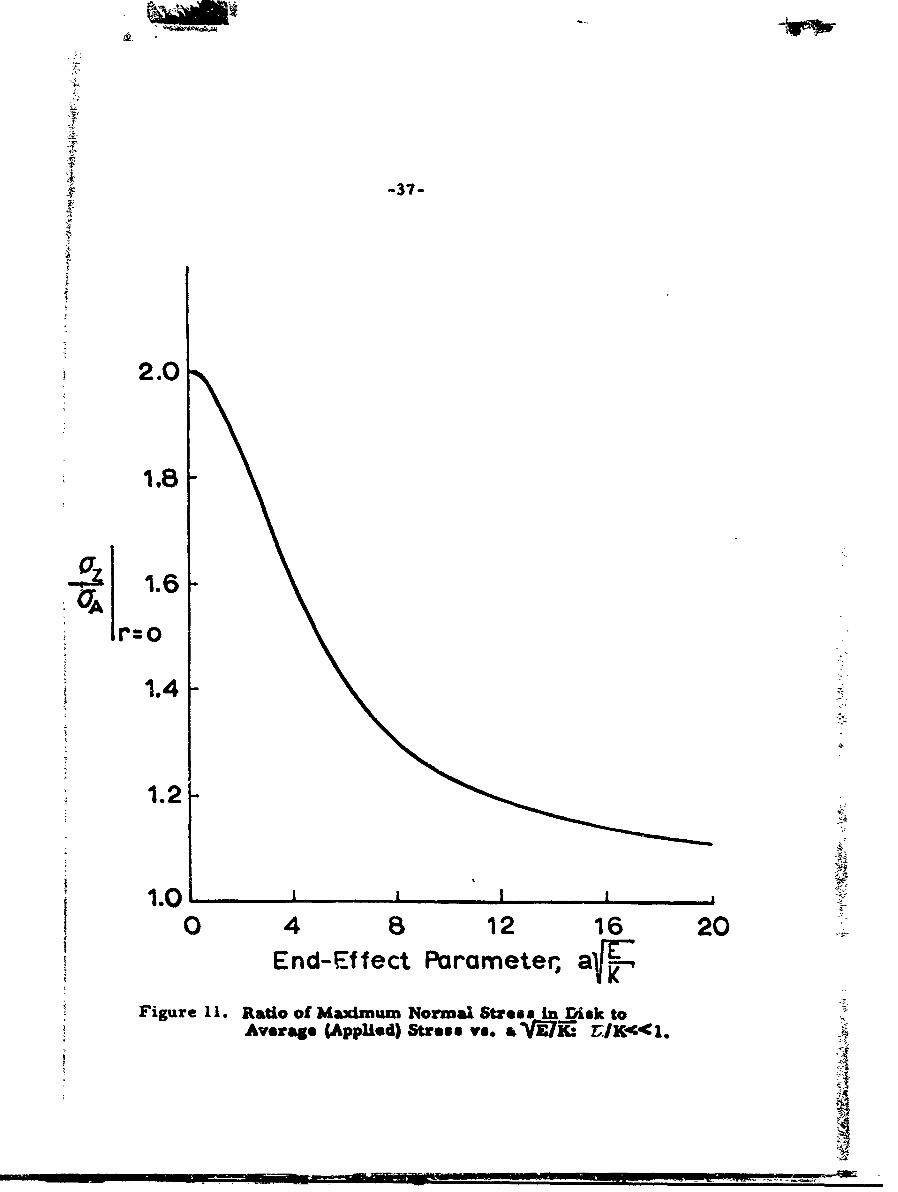
End Effect Parameter
By forming a ratio of expression (2.21) and (2.17b) a measure
of the multiplicity of the local hydrostatic stress over the average
applied stress can be obtained.
z AE 0 (2.22)
- _---r--/-r-

-35-
(1>
0 0ID) C~j
tf-)
CL6f) A,
N V
OD W~ V0M0 OD 0
4o"4
-36-
By evaluating this quantity at a given location in the specimen, the
effect of aspect ratio can be plotted versus material parameters.
Figur-: i is the result for the center of the poker-chip and is quite
usefui as an aid for acquiring an intuitive feel of the geometrical
effects. The abscissa is plotted for values of a greater than or
equal to about fifteen. In other words the limit conditions for
aN'7K- -0 would represent an incompressible material, not a
uniaxial tensile specimen. For most elastomers the ratio of max-
imum normal stress to the average applied stress will be in the
range of 1.8 to 2.0.
The Effect of Corner Stress Singularities
The methods of solution just presented or the stresses in
the poker-chip are not able to predict the co.i.ditions at the bound-
aries where the character of the boundary conditions change, the
reason being the presence of stress singularities, which give rise
to large gradients of stress that become averaged out by the global
methods used. Therefore this region has to be investigated by a
different method capable of describing the local character of the
field variables. Such a methrAd was employed by Williams (42,43)
in studies of plates with angular corners, and then extended by him
'o include bimaterial systems. (44) Zak (45) showed that when the
met'iods employed by Williams are extended to bodies of revolution
the same i :sults are obtained as in the case of plane strain. There-
fcre Lindsey and Zak (46) obtained the solution to the poker-chip
problem through thc use of the plane strain configuration of Figure 1Z.
-37-
2.0
1.8
S 1.6UA
r=o
1.4-
1.2
1.00 4 8 12 16 20
End-Effect Parameter,
Figure 11. Ratio of Maximum Normal Stress in Disk toAverage (Applied) Stress vs. a&""K: IK<K:1.
S. . . . . . . . . . . . _,. • , .. • • :""•"•• , • : .. . , I--.. .. ="'4
-38-
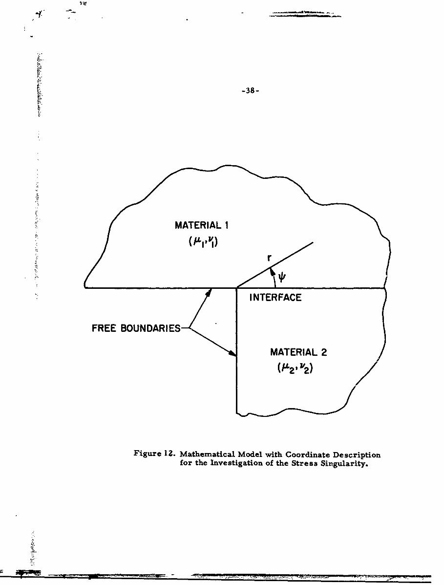
1
MATERIAL 1
S~INTERFACE
FREE BOUNDARIES- /
MATERIAL 2
Figure 1Z. mathematical Model with Coordinate Descriptionfor the Investigation of the Stress Sin1gularity.
317
-39-
i This represents the condition existing at the junction of the free
and rigid boundaries, as shown in Figure 5. Material 1 represents
the grips to which the poker-chip specimen is bonded and Material
Z represents a portion of the specimen near the edge. Material 1
0 0extends over 180 and Material 2 over 90°. This situation cor-
Sresponds to the case where the grips have a larger diameter than
the specimen. A complete analysis of the eigenvalues that produce
Sthe stress singularities is given in Reference (41), including a
matching of the localized singular stresses to the field stresses
obtained by the approximate solution.
COMPARISCN OF RESULTS WITH OTHER SOLUTIONS
Finite Difference
It has been interesting to see how closely the stress distri-
butions obtained from the approximate solution of this section have
been verified by the numerical results subsequently obtained in
Reference (39). Using equations (2. 17) the three average normal
stresses and the shear stress have been computed for the case
a = 10 and v = 0.4 and 0.5, which are configurations analyzed in
Refex -nce (39). The results of this calculation for the axial stress
T are shown in Figure 13, where the stresses obtained from the
two methods of solution are compared. It can be seen fron. these
results that, although the analytical method predicts only the aver-
age normal stress z , the two methods agree very c .,s •ly except
at the edge of the poker chip. At the edges both methods are not
accurate because of the presence of the singularity. The agreement
A
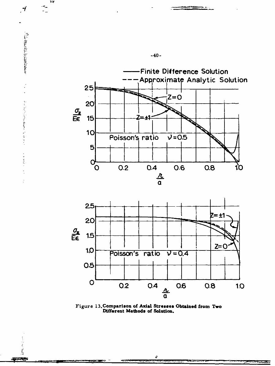
, -40-
Finite Difference Solution--- Ap roximate Analytic Solution
SZo,
2 5 - --
100
10 Poisson's ratio '• 0.5
h510 0.2 0.4 0.6 0.8 ?0
a
2.5---
2.0- -
EX 1.5-
--0 oisson's rati7Vo 4- -0
0.2 0.4A 0.6 0.8 1.0a
Figure 13.Comparison of Axial Stresses Obtained from TwoDifferent Methods of Solution.
t 7 M

for the other three stresses is equally good.
Potential Energy Analysis
In a previous section, an analysis was presented which satis-
fied the displacement boundary conditions, and the z-averaged
equilibrium equations and stress boundary conditions. As such the
solution was expected to be a judicious compromise between a best
deformation (minimum potential energy) and best stress (minimum
complementary energy) approximation. It is informative to inquire
at this point what type solution would result if the potential energy
were minimized, particularly as the deformation functions chosen
earlier, i.e. (2.7), are admissible functions for application of this
theorem. It will be convenient for later purposes to use the dimen-
sionless forms, viz.
u(r,z) = - [1 - (z/hv)2 ] g(r) (2.23a)
w(z) = (wo/hv)z (2. 23b)
where h is the half-thickness of the specimen.V
In the absence of body forces and with zero applied stress
on the stress prescribed boundary r = a, the Minimum Potential
Energy Theorem (47) requires that the potential energy
a h J2
V =S S {Er +Ez] +4+[E +E +62+ dzrdrr.2- (2.24)
v
be a minimum with respect to the variation of functionals involved
in the double integral. Using the expressions for strains (2.8) in
-42-
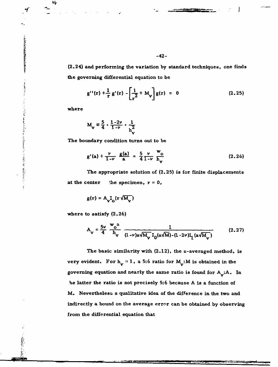
(2.24) and performing the variation by standard techniques, one finds
the governing differential equation to be
g"(r)l+lg'l(r)- + g(r) = 0 (2.25)
"where
M 5 1-2v 1
h•." V
The boundary condition turns out to be
1 g(a g• a W9a a V V a (2.26)
•; v
The appropriate solution of (2.25) is for finite displacements
at the center the specimen, r 0,
g(r) = AvIo(r VW-)
where to satisfy (2.26)
A v w0a (2.27)5v 0w
The basic similarity with (2.12), the z-averaged method, is
very evident. For hv= 1, a 5:6 ratio for M :M is obtained in the
governing equation and nearly the same ratio is found for A :A. Inv
he latter the ratio is not precisely 5:6 because A is a function of
M. Nevertheles& a qualitative idea of the difference in the two and
indirectly a bound on the average error can be obtained by observing
from the differential equation that
-43-
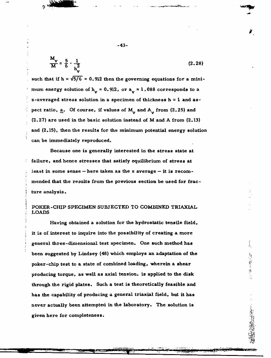
MMj -6-7 (2.28)
such that if h = 4 = 0. 912 then the governing equations for a mini-
mum energy solution of hv 0.912, or a =1.088 corresponds to a
z-averaged stress solution in a specimen of thickness h = 1 and as-
"pect ratio, a. Of course, if values of M and A from (2.25) andSV V
(2.27) are used in the basic solution instead of M and A from (2.13)
and (2.15), then the results for the minimum potential energy solution
can be immediately reproduced.
Because one is generally interested in the stress state at
failure, and hence stresses that satisfy equilibrium of stress at
least in some sense - here taken as the z average - it is recom-
mended that the results from the previous section be used for frac-
ture analysis.
POKER-CHIP SPECIMEN SUBJECTED TO COMBINED TRIAXIAL
LOADS
Having obtained a solution for the hydrostatic tensile field,
" it is of interest to inquire into the possibility of creating a more
general three-dimensional test specimen. One such method has
been suggested by Lindsey (48) which employs an adaptation of the
poker-chip test to a state of combined loading, wherein a shear
producing torque, as well as axial tension, is applied to the disk
through the rigid plates. Such a test is theoretically feasible and
has the capability of producing a general triaxial field, but it has
never actually been attempted in the laboratory. The solution is
given here for completeness.
- --0-0

-44-
The idea is to superpose upon the axial extension of the poker-
chip a torque about its longitudinal axis that will produce a shift in
the magnitude and direction of the principal stresses. The result
will be a general triaxial stress state with which failure surfaces
can be more definitely described and with which the actual failure
mechanisms can be studied. With this modification of the poker-
chip test, a wide range of stress fields can be obtained by varying
&-he ratio of angle of twist to axial extension. Consequently, a study
can be made of the change, or constancy, in the appearance, loca-
tion, orientation and initiation level of the initial fracture point.
Torsion of a Circular Cylinder (49)
The definition of the stress field results from combining
the stress fields of pure extension and that of torsion of a circular
cylinder. It will be recalled from classical theory of elasticity
that for a circular cylinder (and only a circular cylinder) a solution
to the torsion problem can be obtained which leaves the lateral
surfaces free of stress and does not warp the cross-section. The
amount of rotation of a point in a cross-section depends upon its
distance from a base of reference which we will take to be z = +1
from Fig. 5.
e = CL (z-1) (2.29)
where a is the twist per unit length. For a pure torque, the only
displacement is
v 0 = rO = ra (z-l) (2.30)
"-i
-45-
The resulting strains are
zra c r =c=yr=y =0 (2.31)
The corresponding system of stresses is
TOz = Gra 0r=O = Gz = TrO = Trz = 0 (2.32)
This solution will now be used in conjunction with the approximate
analytical solution for the poker chip in extension.
Stress Analysis of Combined Torsion and Extension
Following a procedure very similar to the one used previously
on the regular poker chip, the displacement functions are assumed
to be,
2U = -(l-z )g(r) (2.33a)r
v = rci(z-l) (2. 33b)
w = Ez (2. 33c)
In (2• 33) the displacement boundary conditions are satisfied
at surfaces z = ±1 and g(r) is presently an unprescribed function of
the radius. The strains corresponding to these displacements are
found to beOUr 2
-ra = -(l -z )g' (r) (2. 34a)Ur = rr
r -(l-z 2 ) (2. 34b)
E -= E (2. 34c)
MEMO"---

-46-
ve =o (2. 34d)
Yrr
ave (2. 34e)Ye z z c
OuYrz = = zzg(r) (2. 34f)
from which the z averaged normal stresses are found as
a-$• rrdz X(c -g'(r) - r) 4Gg (r) (Z. 35a)
T0 = $ rdz = ( -4g'(r) - ) - . G (2. 35b)
a ' =d z = g - (g'r ) -+ ( 2 . 3 5 c )
-1
As will be seen from the equilibrium equation, it is not necessary
to average the shear stresses from the equilibrium equation,
" r0 = 0 (2.35d)
" rz = ZGg(r)z (Z. 35e)
" Oz = Gru (2. 35f)
The radial equilibrium equation is satisfied on the average as before
with the tangential expression becoming,
1 a 8Oy z 1d1 (2.36)d=[ 8 ] = 0(. 6
-l -
However, "'Oz = Gra and is not dependent upon z. The third equi-
librium equation is satisfied identically due to the symmetry of the

specimen and applied load about the midplane, z 0. Thus the dif-
ferential equation for g(r) remains unchanged
g"(r + gI'(r) (--2 + M) g(r) = 0r
rwhere (2. 37)
3G 3 (1-ZZv)X+Z = G 2 (I-i'
Now it can be seen that the v 0 displacement arising from the torsion
portion of the load produces no effect upon any of the field quantities
from the approximate solution for the regular poker-chip. Therefore
the two loads are superposable just as they would be for exact solu-
tion of infinitesimal theory. The normal stresses for the combined
loading, valid everywhere except near the edges, become the same
as before for a regular poker-chip, equation (2. 17), and the shear
stresses become,
lz 3v E 1 z (2. 38a)
[1I0(a 4Z) Jo"z r P=2 (2. 38b)EC Z(l+v) C
Principal Stres ses
By seeking for an orientation of stress such that the surface
traction is perpendicular to the surface and no shearing stress exists,
one obtains an equation of the form,
where a, represents the principal stresses. Expanding the determi-
inant
3-( -) 2 22 Z_•a, 3 (a- + W + Wa- ) +- a-rr- +a +Z - -T 2- 2-T z)0-1r 0 z r r zO rO Toz rz
2- 2
Simplifying to the situation at hand and nondi_,ýensionalizing the
• :• principal stresses S =
S3 (27a i)S+[ +2ir z(TO2 2 S
r2• z -T? rz z ITZ r• (E = o z. C)
-r(To 7-+ Tr ) =0 (.1
Substituting equations (Z. 17) and (2.38) into this expression and
solving the cubic equation for S, we obtain the plots of Figs. 14
to 18.
Observations
There are several things to be noted from this solution, one
of which is the fact that for angles of twist that can be classified P.s
being in the range of infinitesimal displacements, the hydrostatic
condition can be altered considerably. For example a typical mater-
al with E = 500 psi subjected to r = .005 and a = 0.1 rad, S1 =10
psi, S2 = 92 psi, S3 = 177 psi at r = 10. Thus a large variety of
stress fields can be readily obtained; however, for failure studies
Fig. 16 shows that P > 2 must be used in order to obtain stresses
larger than the hydrostatic field in the center. In other words, if
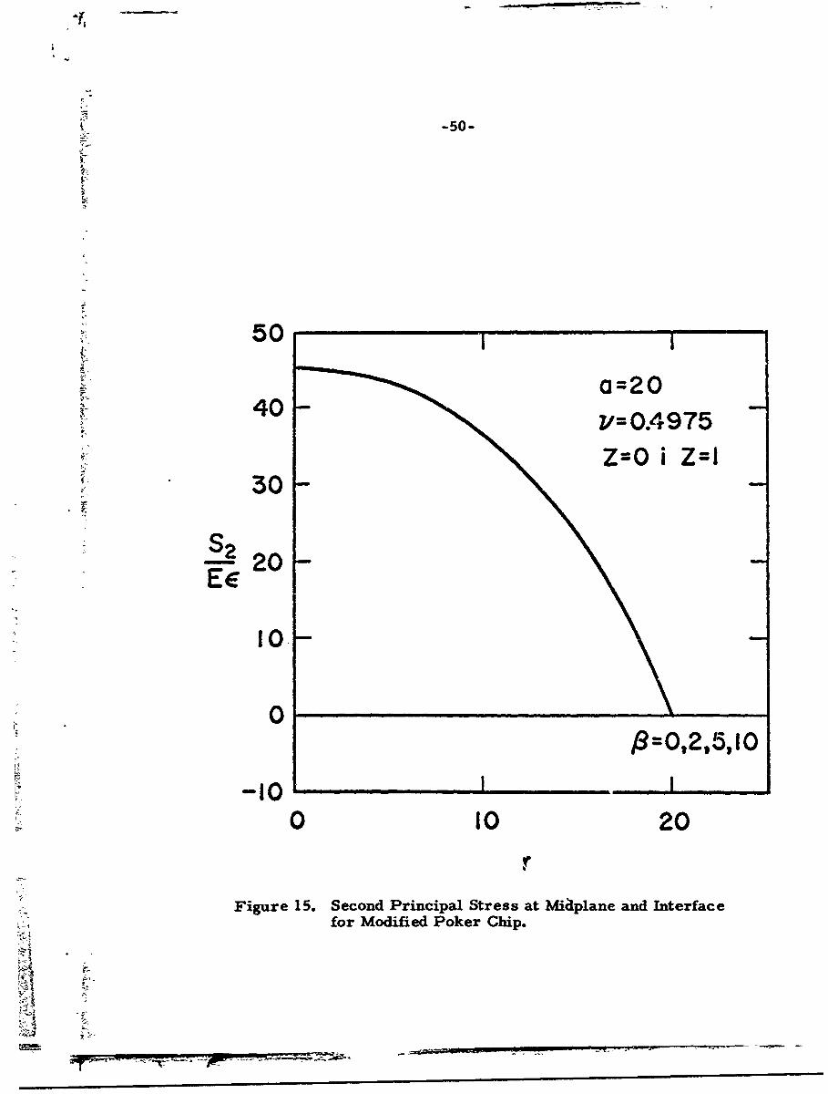
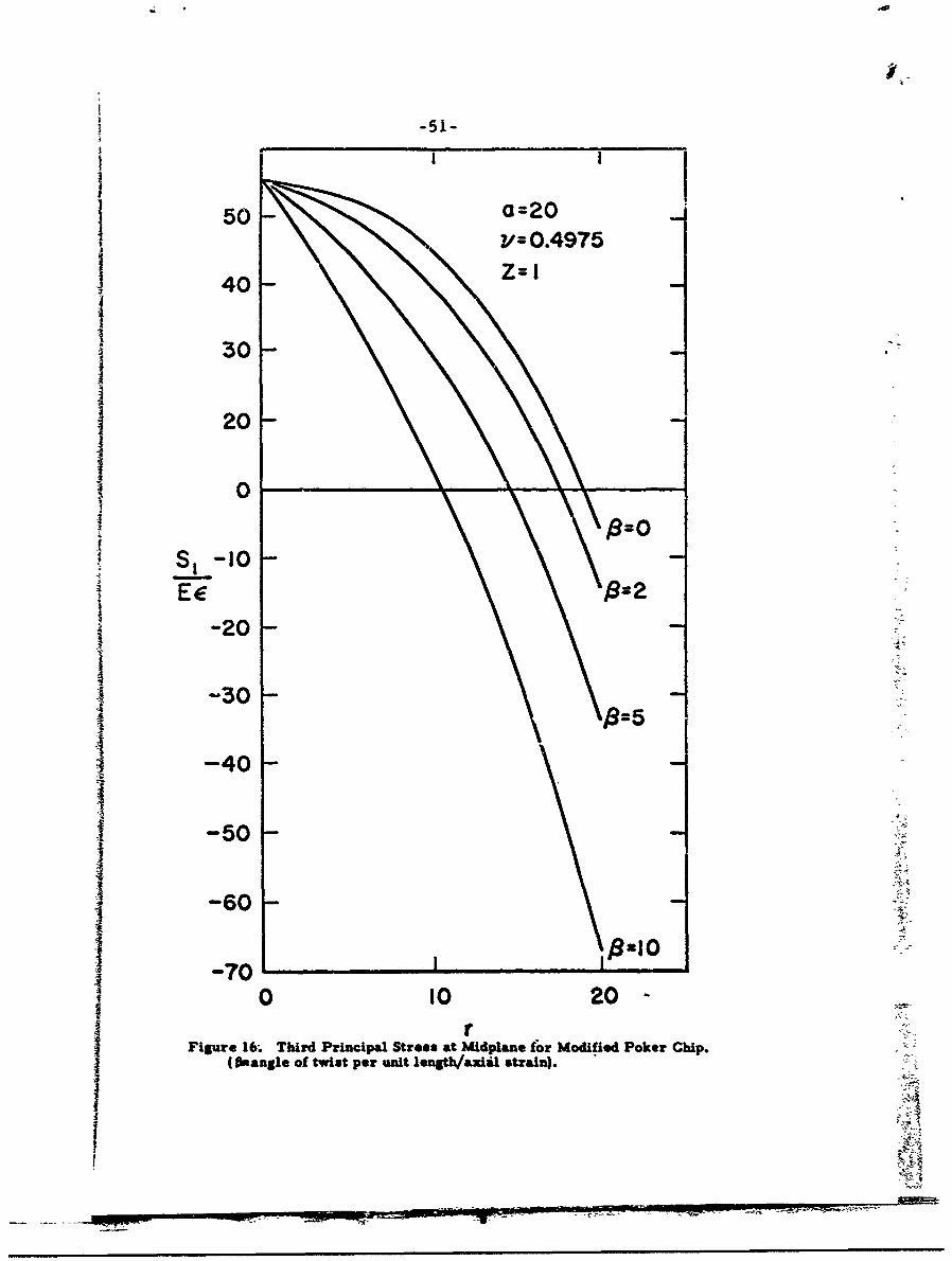
-49-
50
40 1Y=0.4975
30 Z=0 (mid plane)
20
100
0
-20
-30
-40
-50
-60 31
-700 10 20
Figure 14. First Principal Stress at Midplane for Modified Poker Chip.f ~(Ouangle of twist per unit length/aial strain).
! 3A
~ ~ r - -: -7 -
-50-
50
0=2040- 7/= 0975
z=0 i Z=I30
S2
Ec 2 0 -
10-
0
o .. .0.. .5,10
0 10 20
Figure 15. Second Principal Stress at Miaplane and Interfacefor Modified Poker Chip.
tam,
-5'-
50 -t| 0=20
z/=0.4975
4 0 -i30I-
20-
0\820
Ee 48:2
.20
8=54-40
-50
-60
-701 ,!,00 10 20-
rFigure 16-. Third Principal Stress at Midplane for Modified Poker Chip.
(PInangle of twist per unit length/axial strain).
IlI['"-.----

-5-
4so
70k..
60
50
S3 40
30
a=20
20 2/=0.4975
10.8=
0-0 10 20
r
Figure 17. First Principal Stress at Interface for Modified Poker Chip.(Pa'angle of twist per unit length/axial strain).
-77 -7 7
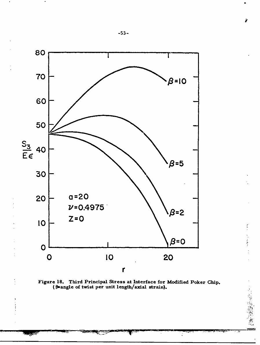
80
70 - .8=10
60
50-
S3E4 0 -
30-
l'=0.4975*
10 z=0
0 /=
0 10 20r
Figure 18. Third Principal Stress at Interface for Modified Poker Chip.(Omangle of twist per unit length/axial strain).
S~-54
< < 2 the largest stresses occur at the center of the specimen where
there is always hydrostatic tension, so in order to produce fractures
t under other conditions 1 must be greater than 2.
As can be seen from Fig. 17, one compo_ýent of ihe triaxial
field can be made compressive. This will provide for failure studies
in the + + - quadrant of the failure surface. Little, if any, work has
been done in this quadrant because of experimental difficulties, but
now barring unforeseen laboratory difficulties this failure surface
can be constructed.
One last observation is made from comparing Figs. 15 and
17 and Figs. 1 4 and 18. For 3> 2 the stress distribution at the mid-
plane is identical to that at the interface of the specimen and the
lucite grips. The stress field is virtually constant through the thick-
ness in the central regions a thickness distance in from the edge.
SUMMARY
In summary it may be stated that these analyses have served
to demonstrate the feasibility of pedducing a state of hydrostatic
tension in soft nearly incompressible materials. They have also
opened the possibility of creatiag a rather general state of three-
dimensional tensile stress, useful in the study of failure surfaces.
Furthermore a detailed definition of the field variables has been
obtained, suitable for use in the reduction and evaluation of exper-
imental data. As a side benefit, a means for measuring bulk
properties in tension has been developed. This i-! not only a con-
venient method of obtaining such informatior but correlation can
-55-
now be made with compressive values, obtained from the more
classical tests, for better definition of material behavior.
T -AXT
-56-
CHAPTER M
EXPERIMENTAL ANALYSIS IN HYDROSTATIC TENSION
MATERIAL DESCRIPTION
The selection, procurement and characterization of an
appropriate material areprerequisite to experimental investigation.
This always involves a compromise as one tries to find typical
materials that are readily available and yet still possessing mater-
ial properties that are.amenable to standard laboratory testing.
There is currently in progress a program (50) to find one or more
rubber materials suitable as standards for all interested investi-
gators to use as a basis for interchange of information. One of
the candidates under study is a polyurethane elastomer of a type
employed as propellant binders. It is commercially produced by
the Thiokol Chemical Corporation under the trade name of Solithane
113 (S-113). Chemically, urethane polymers are the product of a
reaction between an isocyanate and a hydroxyl radical. Normally
the process consists of three steps: prepolymer formation,
chain extension, and curing. Although the specific formulation
of S-113 is company proprietary, some general statements can
be made about it. Quoting extensively from "Polyurethanes:
Chemistry and Technology," (51) with occasional annotations, we
will discuss the three steps.
Prepolymer Formation
The reaction of a diisocyanate with a hydroxyl-terminated polyester, polyester amide, or polyetherto form an isocyanate-terminated prepolymer canbe represented schematically as follows:
-7-

7-57-
"OCN-R-NCO + HO--OH -
diisocyanate polyester or polyether
0 0
OCN-R-NH- L-O-0NH-R-NC0
prepolymer
For S-113 the diisocyanate radical R was Tolilene, TDI. After the
b asic links are formed, they are used as building blocks to form
Iextended chains.
Chain Extension
Chain extension of the prepolymer with active hydrogen-containing compounds, usually difunctional, such as water,glycols, diamines, or aminoalcohols, proceeds to give ahigher molecular weight, soluble polymer. Chain extensionwith glycols takes place with the formation of urethanegroups as shown below:
0 0
ZOCN-R-NH- --C0 C--NH-R--NCO + HO-R'--OH -glycol
i urethane
OI -- R
OCN-R-NH- .w.......0- H-R NH-
For S-113 the extension agent R' is Polypropylene glycol, PPG.
Thus far chain extension has been shown wherein anexcess of isocyanate was used, giving an NCO-terminatedpolymer. These polymers are actually high molecularweight polyisocyanates, and as such are reactive withmany chemicals, hence are not indefinitely stable. Solu-ble polymers of better stability may be prepared, ifdesired, by using a slight excess of the active hydrogen N4
-~ - rw ~ 7 ->MP

-58-
comp ýnent, rather than an excess of isocyanate. Forexample, an excess of glycol would lead to a polyure-thane terminating in hydroxyl groups, and would hencebe much more stable.
2 OCN-R-NHCOO--OCONH-R-NCO + 3 HO-R 1-OH -.
HO-fR '-OCONH-R-NHCOO--.•OCONH-R-NHCO RIR-OH
Other active hydrogen compounds could be used similarly,but hydroxyl compounds usually serve as the best chainterminators, free from other complicating side reactions.
Curing or Crosslinking
The curing or crosslinking of the elastomer may beaccomplished by reacting an added curing agent withthe intermediate molecular weight elastomer, or byformulating the elastomer so that it contains free iso-cyanate groups and curing by heating.
A convenient means of introducing crosslinking inthe urethane polymer chain is the use of triols, eitherin forin of monomeric polyols such as trimetholylpro-pane or by employing poly(oxypropylene) glycol deriva-tives of triols such as trimethylolpropane, glycerol,and others. In this case, crosslinking occurs throughthe formation of urethane links as shown below:
0 0 OH
OCN-R-NTHI-OýO NH-R-NCO + HOLOHtriol
-- O NH--R-i-NH-0ýOI urethane crosslink
-R-NH-Li-oX"NH-R-
The catalytic triol used in S-113 was Thiokol catalyst C113-300 and
curing was prescribed at 1500C.
S-113 can be made with widely different mechanical proper-
ties by varying the relative amounts of the prepolymer and catalyst.
VIM= , -
-59-
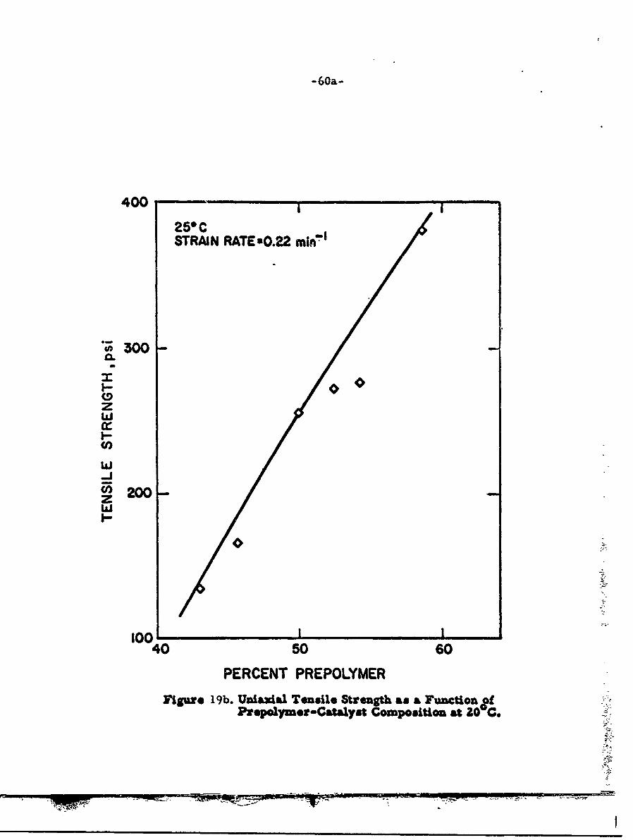
A study by Knauss (50) shows the degree of sensitivity, which is
graphically displayed in Figure 19. The ratio used in this program
was one to one by volume, which was found by testing other pro-
portions to be the most suitable for this investigation.
MATERIAL FABRICATION
A very detailed account of material fabrication along with
descriptive photographs and schematics of the equipment has been
given by Zak. (51) Briefly the process may be described by stating
that the two separate components, prepolymer and catalyst, were
preheated to 600 C while they were in an inert atmosphere of nitro-
gen. They were then carefully measured by volume and mixed
together, still under nitrogen, and raised to 1000C. The mix was
degassed for five minutes, which acted to reduce virtually to zero
the number of visible bubbles produced in the casting, and further-
more it tended to make the finished product more nearly colorless.
A mold of polished aluminum was preheated in the oven to 125°C,
and it should be emphasized that no mold release was ever used in
the fabrication process. It was found impossible to remove com-
pletely the residue left by the release regardless of the solvent
used, and the contamination of the surface prevented the formation
of a good bond. A polished mold face was found very acceptable
for releasing the specimen. Polished brass, steel and aluminum
as well as Pyrex glass, and Micarta were used, but polished alumi-
num was found to be the most desirable when all of the factors of
cost, weight, etc. were considered. The surface quality of the
S :: :a : - -- -

-60-
300 I
3Go
200
100
60-
40 - G" -
20-40[
40 50 60
PERCENT OF PREPOLYMER
Figure 19a.Complex Modulus at ZO0C as a Function of]Psepolymer-Catalyst Composition.
T
-60a-
400,,I
25°CSTRAIN RATE ,0.22 mmr'a
"5 300
zwI-v(09
w-Jr 200-z
fr- O
100 I
40 50 60
PERCENT PREPOLYMER
Figure 19b. Uni&hdal Tensile Strength as a Function ofPrepolymr-Catulyst Comnpositioa at 30 C.
7 7'
-yr
/
:S
j -61-
cast sheet is directly related to the surface quality of the mold, buL
as will be discussed later when the material is bonded to the lucite
grips, the wetting properties of the bonding agent eradicate surface
imperfections in the cast sheet. Therefore the mold surface need
be polished only to the degree necessary to allow the rubber to be
removed from the mold.
With the mix up to temperature and degassed, the molds
were filled through tubular arrangements while they were in the
oven, so that the material was never exposed to the atmosphere.
The reason for the great care was tD prevent side reactions that can
be produced by water.
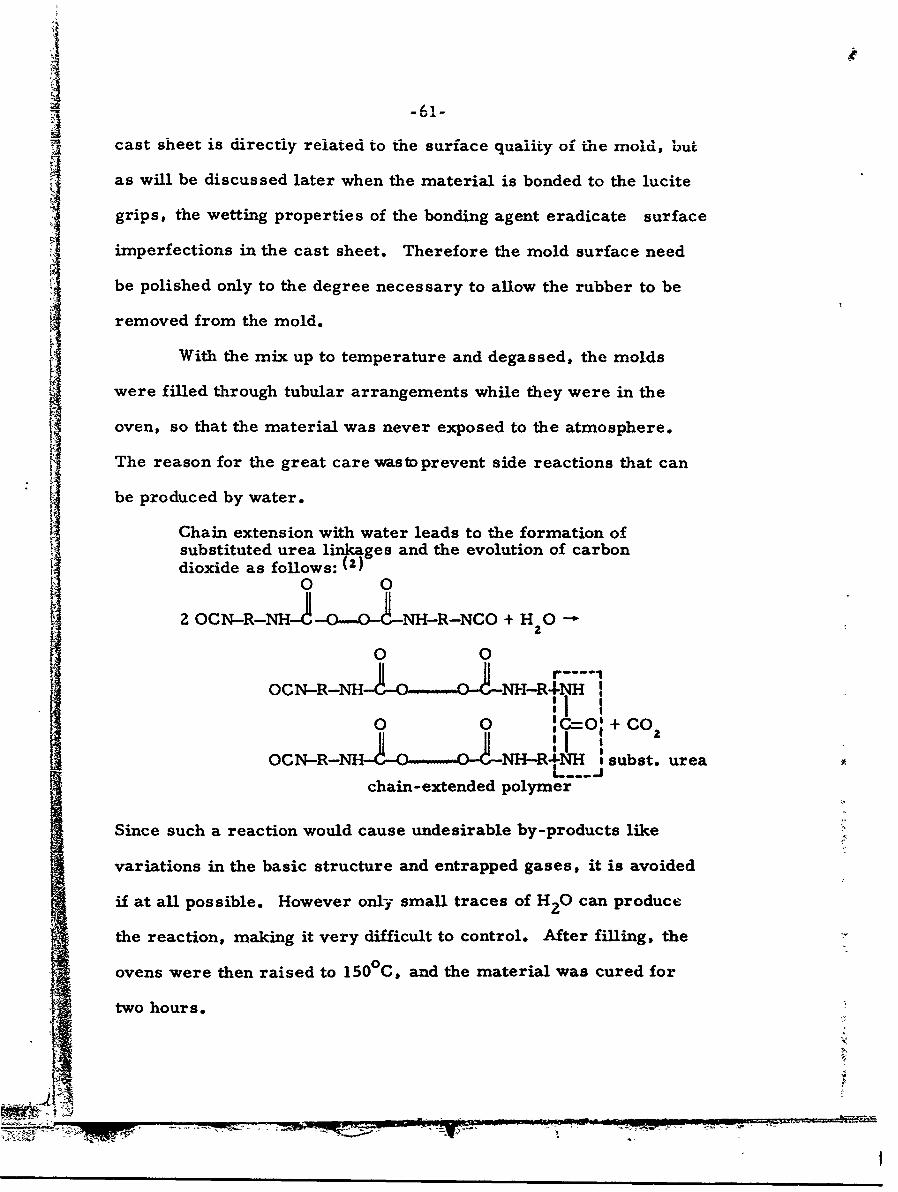
Chain extension with water leads to the formation ofsubstituted urea linkages and the evolution of carbondioxide as follows: (2)
0 0
2 OCN-R-NHJ -01NH-R-NCO + H 0-
0 0
OCN-R--NH-C. NH-R4NH
0 0 1C=O' + CO2
OCN-R--NH-%-O.-....--!-NH-R1NH subst. ureachain-extended polymer
Since such a reaction would cause undesirable by-products like
variations in the basic structure and entrapped gases, it is avoided
if at all possible. However only small traces of H2 0 can produce
the reaction, making it very difficult to control. After filling, the
ovens were then raised to 150 0 C, and the material was cured for
two hours.
00 . . .. . . =- *••-•=-•--
-62-
Every effort was made to closely control each step of the
process; however due to the fact that several very complex chemical
reactions are taking place simultaneously, it is difficult to produce
polyurethane with low batch to batch variability. This problem has
been alleviated somewhat with a correlation between modulus and
percentage of prepolymer in the mix. (See Figure 19.) By cutting
a test strip from each casting, the material can be quickly evaluated
by means of its modulus. Thus a uniform set of specimens can be
gathered and variations due to slight modifications in the basic mix
can be quickly detected. Scatter ranges are discussed under Mater-
ial Characterization.
After curing was complete,the material was removed from
the mold and placed in a dry box for two weeks or until used. The
final product was a large round sheet 13 inches in diameter and
0. 10" thick. When ready the smaller poker-chips were then cut
into disks of approximately 2-1/z" in diameter. The resulting
material specimen was virtually clear, which is one of the primary
reasons for selection of S-113. It allows the possibility of either
viewing directly, or photographing, the internal fracture process
as it happens. This is a great advantage, for it is normally very
difficult to surmise accurately what has happened during fracture
solely from looking at the surface after the fact. Furthermore the
material is optically very sensitive, and ideally suited for bire-
fringence work. This property has been characterized and is alluded
to in the discussion of material characterization.
-63-
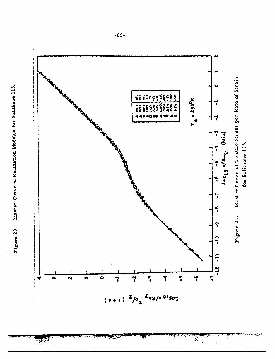
MATERIAL CHARACTERIZATION
The characterization of S- 113 has received the attention of
several investigators including Williams, Ferguson, and Arenz (52)
as well as Knauss, (53) and Zak. (54) These include various me-
chanical property definitions under infinitesimal strains, including
a rather complete description of viscoelastic properties which even
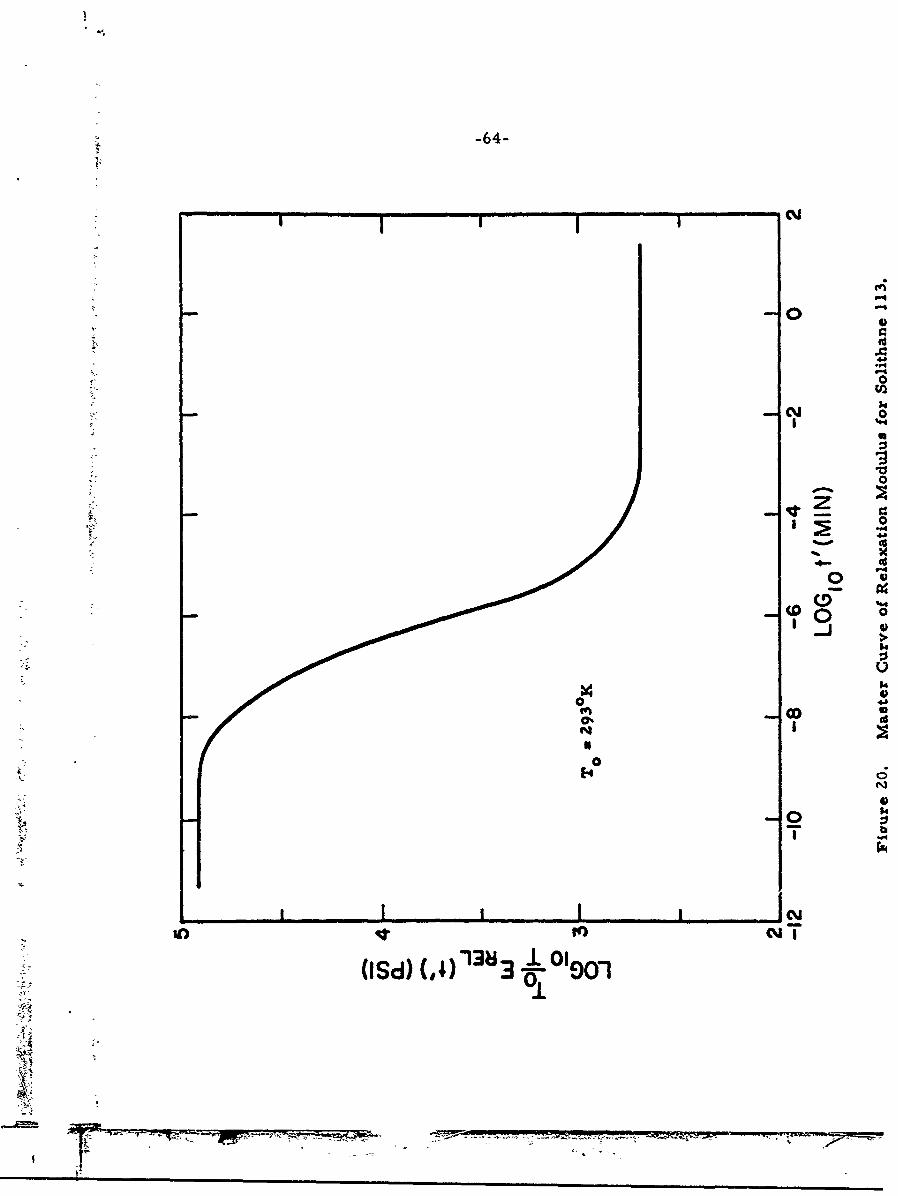
encompasses the optical properties of birefringence. Figures 20
to 22 give information relating to the constitutive properties of
S-1 13 in the form of the Relaxation Modulus, the Master Stress-
Strain curve and the accompanying shift factor for them. The data
was obtained using standard techniques primarily based on the
constant strain rate test. The relationship between the constant
strain rate response and the relaxation modulus is straightforward
and can be derived as follows. For a linear viscoelastic material
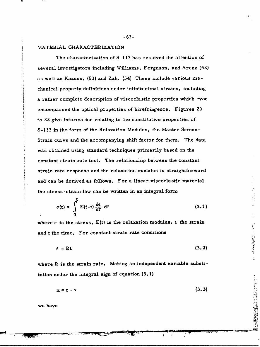
the stress-strain law can be written in an integral form
t
Olt) = C E(t-T)) dT (3.1
0
where T is the stress, E(t) is the relaxation modulus, e the strain
and t the time. For constant strain rate conditions
= Rt (3.2)
where R is the strain rate. Making an independent variable substiX
tution under the integral sign of equation (3. 1)
x= t T (3.3)
we have
-64-
004
o pV
0
14
I '.4
coS
00
$4.
CDj
1384
(I Sd)310100
-65-
U))
0
04
0 r0
'lo
P4K
o $4
opR4h4
44
Ix b 0
c'Jn
-,4.
ap00
w o ctoo-2z 0
0 5 0
00 w
f~$4
ID 01 90-

-67 -
talt) = -R Y E(x) dx (3.4)
0
From equation (3.4) it follows that
1 d t) E(t) (3.5)
Equation 3.5 shows that the relaxation modulus for a linear visco-
elastic material is equal to the time rate of change of stress divided
by the strain rate in a constant strain rate test. This relationship
is used to evaluate the relaxation modulus from the data of the con-
* stant strain rate tests. The tests were performed for a wide range
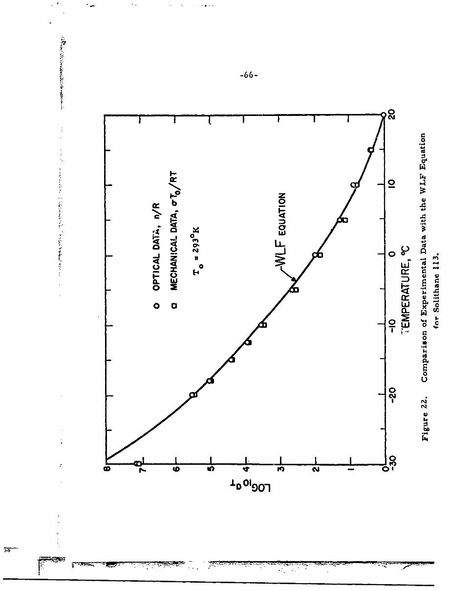
S"2 of rates and temperatures and then shifted (55) by the aT factor de-
.4 scribed in Figure 22 to give the composite master curves of FiguresV'
0 20 and 21. The mechanics of data representation, interconversion,
04 etc. is involved, but now reduced to standard practice as described
0* in detail by Arenz, Ferguson, Kunio, Williams. (56) The curves14-
indicate something of the nature of the material; however, the par-P4
o ticular quantity to be noted at this time is the rubbery modulus of
I approximately 500 psi, which will be used in data reduction for the
elastic analysis. Zak, (54) using an experimental technique sug-
gested by Smith, (57) demonstrated that constant-strain rate tests
i at 0.02 in/min. and T = 25 0 C, were in the rubbery regions for S-113.
This is the test condition used in the experiments to be described
subsequently; consequently E = 500 psi is the pertinent materialp
S parameter.
I -68-
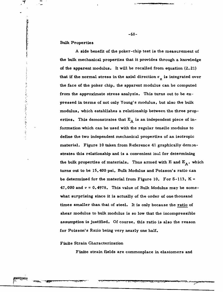
Bulk Properties
A side benefit of the poker-chip test is the measurement of
the bulk mechanical properties that it provides through a knowledge
of the apparent modulus. It will be recalled from equation (2.21)
that if the normal stress in the axial direction a is integrated over
the face of the poker chip, the apparent modulus can be computed
from the approximate stress analysis. This turns out to be ex-
pressed in terms of not only Young's modulus, but also the bulk
modulus, which establishes a relationship between the three prop-
erties. This demonstrates that EA is an independent piece of in-
formation which can be used with the regular tensile modulus to
define the two independent mechanical properties of an isotropic
material_- Figure 10 taken from Reference 41 graphically demon-
strates this relationship and is a convenient tool for determining
the bulk properties of materials. Thus armed with E and EA, which
turns out to be 15,400 psi, Bulk Modulus and Poisson's ratio can
be determined for the material from Figure 10. For S-113, K =
47,000 and v = 0. 4978. This value of Bulk Modulus may be some-
what surprising since it is actually of the order of one thousand
times smaller than that of steel. It is only because the ratio of
shear modulus to bulk modulus is so low that the incompressible
assumption is justified. Of course, this ratio is also the reason
for Poisson's Ratio being very nearly one hall.
Finite Strain Characterization
Finite strain fields are commonplace in elastomers and
-'- . -, - ,

-69-
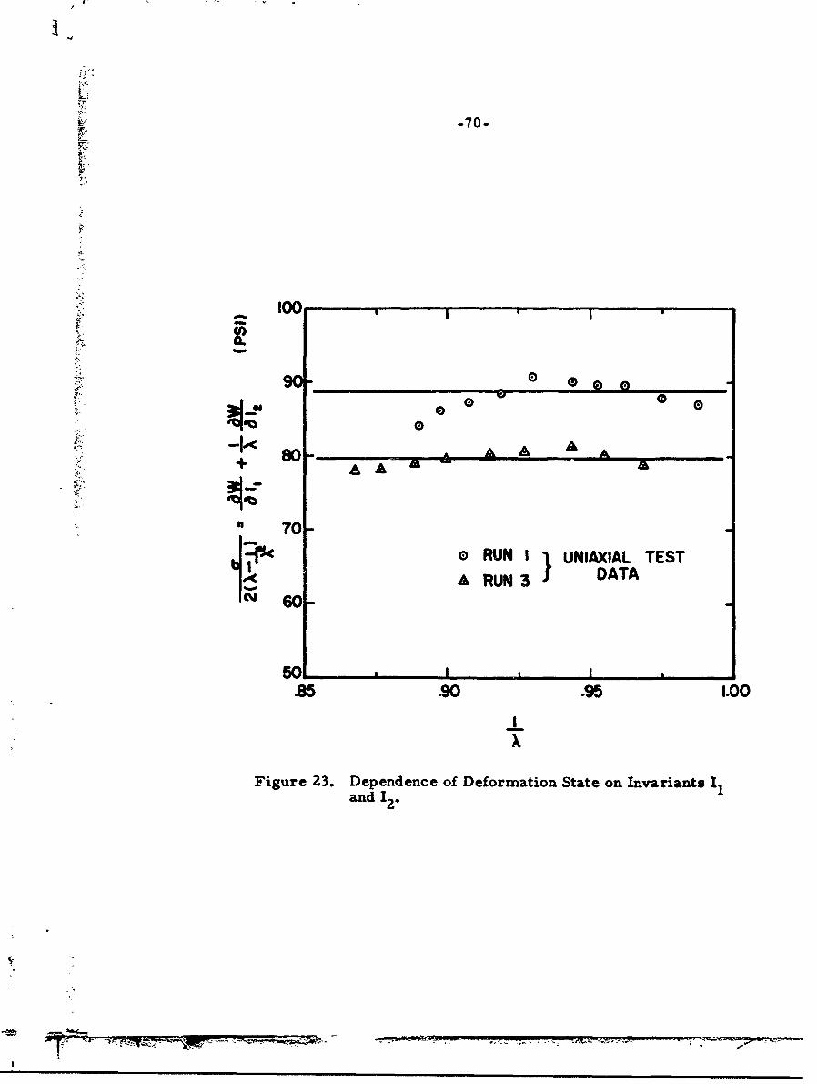
require a special characterization for the material subjected to
them. (4) Both uniaxial and biaxial tests have been conducted by
Beckwith and Lindsey (58) to determine the form of the strain
energy function, W. It is customary to express W as a function
of the three strain invariants
II =2 2 (3.6a)
1 22+ 2 2 2 2 (3 6b)12 = + YIX3 + X2X3
13 2 222 (3. 60
where k's are stretch ratios. When the material is incompressible
13 i, and
W = W(I , 12 )
For the case of uniaxial tension A X and X2 =)3 = -1/2
and the corresponding tensile stress is (4)
= 2(k_X- 2 ) (aw + I OW (3.7)
By dividing out the first factor and plotting it versus 1/X and using
experimental data from a uniaxial strip, we obtain Figure 23. (The
two sets of data points demonstrate maximum batch to batch varia-
bility.) From the trend of the data it can be inferred that the inter-
cept, OW/IiO, is constant and the slope, 8W/8I2 J is zero. The
strain energy function m•_ust then be of the form
W = Ci(1,-3) (3.8)
- -I
-70-
___ 100,I
S900
0 0:: -k 80-.
+ AA& A A A
"70
0RUN I 1UN IAXIAL TESTA RUN 3 DATA
501.85 .90 .95 1.00
Figure 23. Dependence of Deformation State on Invariants Iand 12.

-71-
state; i.e., X. = 1. This classifies the finite strain behavior of1
S-113 as Neo-Hookean, which is the simplest representation and
a naark in its favor. Simplicity in analysis is a big asset in large
deformation problems.
Now to see exactly how close S-1lI 3 folows Neo-Hookean
behavior in uniaxial tension, Figure 24 has been plotted. Only in
the larger values of stretch ratio near fracture is there any per-
ceptible deviation. Also the value of the material constants agree
well with the infinitesimal limit case, which defines C1 = E/6.
Corroboration of the Neo-Hookean result based on uniaxial
test was made from equal biaxial tests on the test rig pictured in
Figure 4. In this case A, = X2 = X and X3 = )-2 from the incom-
pressibility condition. The corresponding in-plane stress turns
out to be (4)
W R=2 -)-6 + X w(3.9)
where p = internal applied pressure
R = radius of curvatur6
t = sheet thickness
Proceeding upon the assumption that S-11 3 is Neo-Hookean, equa-
tion (3.9) becomes
'= C 1 1 -U 6) (3.10)
Assuming a circular arc deflection curve, the radius of curvature
for a sheet of original radius a and pole height h (see Figure 4) is
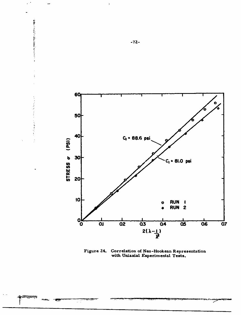
I7
6 e00
50-
40 C, 88.6 ps
0.
"b 30- C,8•,.0 psi
20O
10 * RUN I.RUN 2
01L0 oj 02 G3 04 05 06 (7
Figure 24. Correlation of Neo-Hookean Representationwith Uniaxial Experimental Tests.
-73-
R h (3.11)-2h
Giving
pa2 +h2 -6Bht C1 (1-4-6 (3.12)
By measuring p, h and X it was possible to construct Figure 25 for
an initial sheet radius of five inches. The plot indicates a linear
relation except in the initial stages of deformation. It was definitely
established that the nonlinearity was due to slippage of the sheet
underneath the clamping ring making the measured value of h too
large. The ring is not fastened down too tightly since premature
fracture at the grip will ruin the test. After the initial slippage the
curve then becomes linear to establish Neo-Hookean behavior.
EXPERIMENTAL APPARATUS FOR THE POKER-CHIP TEST
As the equations and figures of Chapter H demonstrate, the
poker-chip test constitutes a vehicle by which a hydrostatic tensile
field can be applied to a local region of a body whose actual dimen-
sion is dictated by experimental practicality. The theoretical
analysis shows that an aspect ratio of fifteen to one is the lower
limit required to produce this stress field and twenty to one is
more desirable. A two-inch diameter with 0.10 inch thickness
was selected to be a reasonable compromise between what could
be effectively bonded and pulled and what was desired in the way
of observation. Although Gent and Lindley originally performed
the poker-chip test by pulling or squeezing rubber blocks between
A> - - -mpg
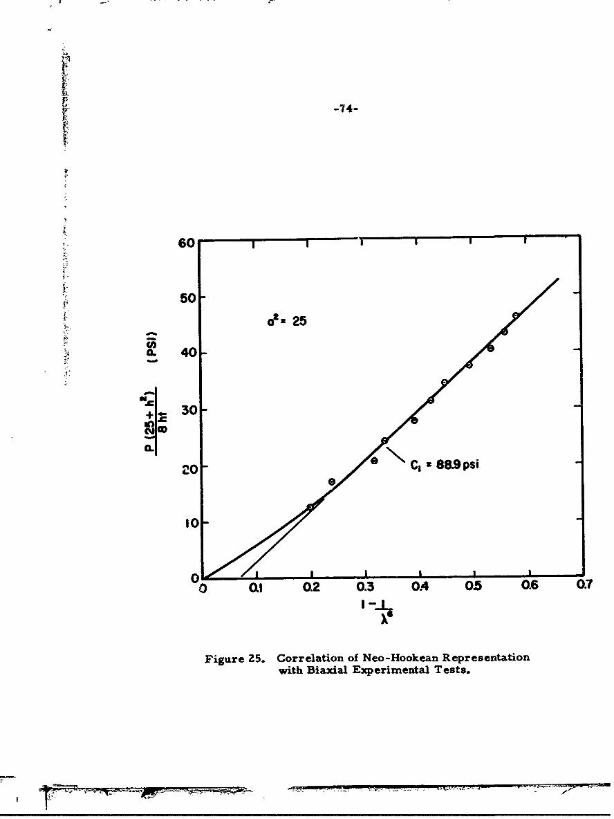
-74-
60 1
"50
at? 25
0. 40-
"•• 30-
in=
20 C, X 88.9psi"
100
0 0.2 0.3 0.4 05 0.6 0.7
Figure Z5. Correlation of Neo-Hookean Representationwith Biaxial Experimental Tests.
OT 1M -- T

-'7 5-
steel plates, it was decided for the experimental work on S-I1 3
that the apparatus would be altered considerably to facilitate a
more thorough study of the actual mrrechanisms of the fracture pro-
cess. This was accomplished by using transparent lucite grips
in place of steel. Lucite has a .nodulus in the neighborhood of
500,000 psi (59) and this provides approximately a 1,000 to 1 ratio
between modulus of grip and specimen, which closely duplicates
the theoretical assumption of rigid boundaries made in the stress
analysis. Coupled with the clear grip and clear specimen a
transparent bonding agent was found in the form of Eastman 910,
which happily acted as a wetting agent for both the rubber speci-
men and the lucite grip. When the assembly was complete, a
window was produced through which the observer could view the
internal regions of the material and study the fracture process.
A schematic drawing of the entire assembly is shown in Figure
26 where the arrows indicate the attachment of a testing machine
through which the specimen was loaded.
Bonding Procedure
A very critical facet of the experimental technique of
the poker-chip test is the bonding procedure. Being somewhat
of an art, it is demanding upon the technician to produce a bond
with sufficient strength that the specimen will not tear away from
the grip before an internal fracture is produced. The specimen
is prepared by roughly cutting it to size and then cleaning it thor-
oughly with a clth slightly dampened in methyl alcohol. If used
sparingly this procedure will not produce noticeable swelling in
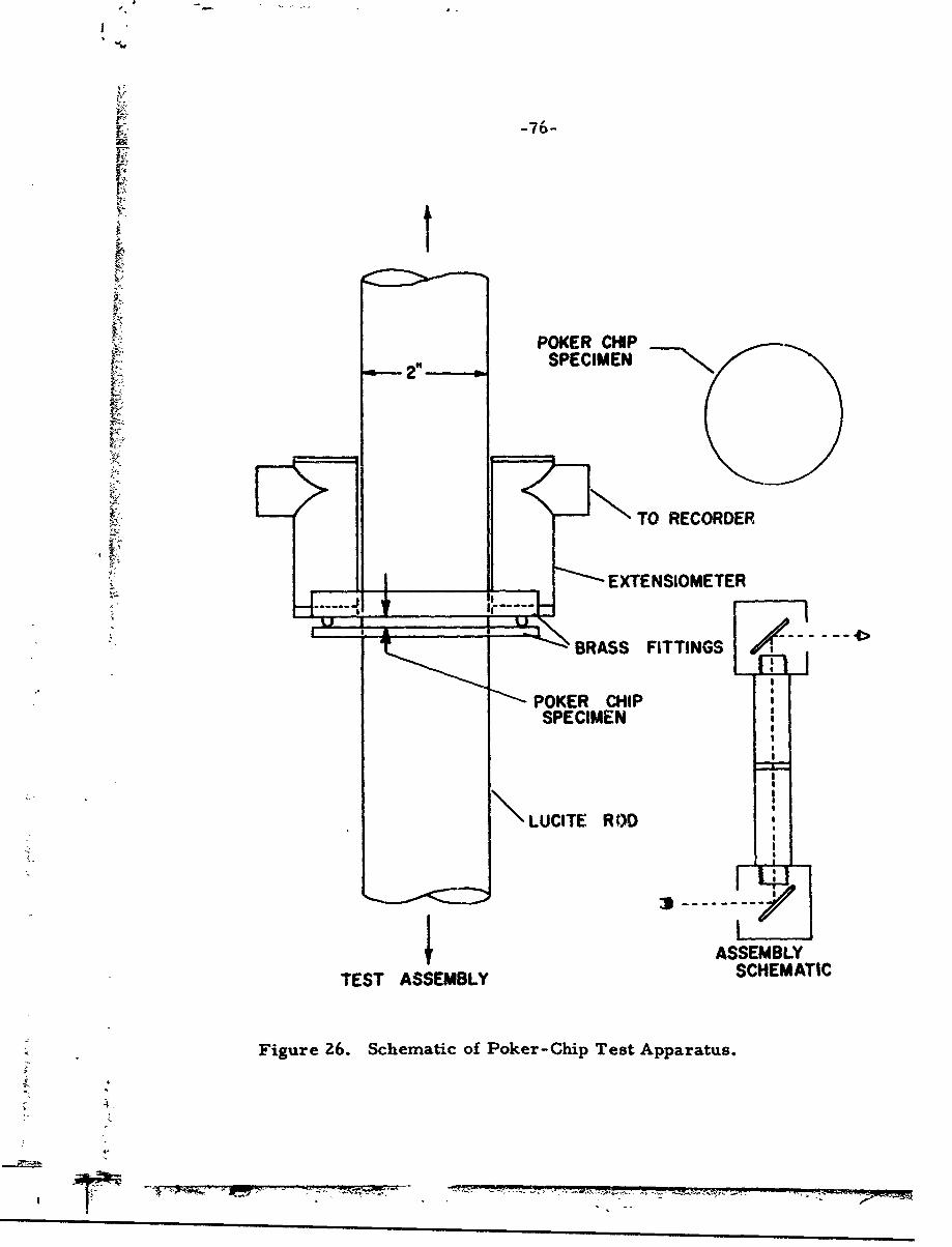
S-76-
POKER CHIP
SPECIMEN
TO RECORDER
"EXTENSIOMETER
BRASS FITTINGS
POKER CHIPSPECIMEN
LUCITE ROD
ASSEMBLYTEST ASSEMBLY SCHEMATIC
Figure 26. Schematic of Poker-Chip Test Apparatus.
4e
-77-
I the rubber. The lucite grips must be lightly roughened an-d thor-
oughly cleaned; furthermore it was found advisable to avoid silicon
compound abrasives, and aluminum oxide paper was found to work
nicely. A bonding accelerator (number GA-IAI) supplied by Eastman
was then applied to the specimen and the Eastman 910 to the grip.
The two pieces are brought together under hand pressure and al-
lowed to set. The process is repeated for the other grip; however
a V-block is used to insure perfect alignment. Absolutely no mis-
alignment can be tolerated due to the bending imposed in the test.
The same is true of taw.er "; the specimen; once bending is present,
the local stress conditions become unknown and the test is of little
use.
Optics
With the specimen bonded to the lucite, the grips were
sc."ewed into special fixtures depicted in Figure 26. Front sur-
fac• mirrors were mounted at 450 to the horizontal in these
head3, providing a periscope arrangement for viewing the spec-
imen. Through one mirror the specimen was illuminated by
means of a Peck model 110 Mercury vapor point source and view-
ing or photographing took place through the other. With this
powerful light source, it is possible to take high speed rmotion
pictures of the fracture process to document a detailed history
of it.
This method has also been successfully used even on
quite opaque and translucent materials. These are not as desirable

-78-
as the clear materials, nor are they as readily photographable, but
fracture initiation is easily detected along with rather gross details
of the propagation phase, depending upon the degree of opaqueness
of the mate;-1l. Furthermore, if the material being tested lends
itself at all to i•e transmission of light, the fracture point can be
detected, for there are in3tances recorded where it has been foaund
difficult to ascertain the point at which the specimen actually failed
because no direct manifestation of it was made on the load his-
tory. (60)
17 Strain Measurements
( One of the many interesting aspects of this test is the fact
that the overall specimen strain based upon the initial thickness is
small; i.e., S-113, which evinces 35 percent to 40 percent ultimate
strain in uniaxial tension, exhibits only two percent to three percent
ultimate strain in hydrostatic tension. This was another reason
for putting faith in the results of the approximate stress analysis
which employed tools of infinitesimal elasticity. It should be pointed
out that this configuration is one of the few wherein infinitesimal
theory can be applied to fracture analysis of rubbery materials with
confidence in the accuracy of the solution. Such a state of affairs
is certainly welcome since use of finite elastic techniques for
analysis is very limited and virtually never used in fracture studies;
however, Levinson and Blatz (61) have employed a variational scheme
to solve the poker-chip problem for large deformations, so that
materials demonstrating strain levels out of the range of the linear
-79-
I: theory or on the border of linear theory can still be analyzed for the
poker-chip test.
Because the displacements were small, for instance in the
tests to be discussed total displacement at the grip was in the neigh-
borhood of 0. 002 inches, extensometers were used to measure the
Saxial separation of the lucite grips. (See Figure 26.) They incor- V
porated linear, variabl4 differential transformers, LVDT, in con-
junction with Schaevitz LVDT exciter, demodulator, type DMPS-3.
SThese operated into a Moseley Autograf, X-Y Recorder, Model
2FR-A(S), made in Pasadena, California, where the displacements
were magnified 2000 times. A photograph of the actual specimen
: with the LVDT's mounted in place is shown in Figure 27. The com-
plete assembly was placed in a Universal Testing Machine, Model
Number TTC, manufactured bV Instron Engineering Corporation of
Canton, Massachusetts. A photograph of the apparatus ready for
test is given in Figure 28.
EXPERIMENTAL RESULTS
With a knowledge of the two independent mechanical proper-
ti-s v and E, Figure 8 can be used tto find the relationship between
the internal field stress in the poker-chip and the externally applied
strain 61 . which of course can in turn be related through the apparent
modulus to the applied load. The load was correlated with the dis-
placement through an apparent stress-strain curve. This was
computed by considering the specimen to be a uniaxial tensile bar
where the stress is obtained by dividing the applied load by the

*1 -SO
Figure Z7. Arrangement of the Triaxial Test.
* ~,-*.

01
Figure 28. General View of the Triaxial Test Showing the Specimens inthe Instron Testing Machine and the Recording Equipment.
'7
-82-
cross-sectional area of a large face, P/A, while the strain is corn-
puted like a tensile bar on the basis of specimen thickness. The
descriptive parameter for this pseudo stress-strain curve is the
apparent modulus, EA, computed in the obvious way by dividing the
equivalent uniaxial stress by the equivalent uniaxial strain. A plot
of several typical apparent stress-strain curves obtained at a strain
rate of 0.02 in/min, is given in Figure 29. showing the rubbery,
elastic response of S-113 in HT. This gives some indication of the
scatter in the apparent modulus due to the batch to batch variability
of the material. Both the mode and the average come out to be
approximately 15,400 psi with a maximum variation of 1±8 percent.
As can be seen, the apparent stress-strain relation is linear
well above one percent strain, and then it bends over as it proceeds
to fracture at strains of 2-1/2 percent to 3 percent. The actual
fracture stress levels involved are considerably higher than their
uniaxial counterparts; however as was discussed previously, the
ultimate strain is greatly reduced. From Figure 8,Oz /aE = 48,
which gives a local HT of 625 psi. S-113 possesses an ultimate
strength in uniaxial tension of approximately 160-200 psi, (62)
while local stress values in the hydrostatic configuration range
approximately three tirnes this value in the neighborhood of 500-650
psi. These values quoted represent the range of a large number of
tests conducted at room temperature.
Stress-Axis Theorem
It is interesting to abstract from this and other work (22)
A

I II
300
EA= 15,300 EA= 14,300
.. 200
Q.
100
0.01 0.02 0.03CA
Figure Z9. Apparent Stress-Strain Curve for PokerChip Test.
-84-
for engineering intuition. It can be stated roughly that as the number
of axes of stress increase the ultimate stress is increased and the
ultimate strain is decreased; furthermore, as the degree of axiality
of stress is altered toward the hydrostatic this same trend will be
emphasized. In other words, as an additional axis of stress is
added to a body in uniaxial tension, the ultimate stress and strain
increase and decrease respectively from the uniaxial value as the
new stress component grows from zero to become equal to the orig-
inal one producing a state of equal biaxial tension. Adding another
axis of stress to the biaxial case further alters the ultimate proper-
ties in the same direction as it grows from zero to become equal to
the original two and produce a state of three-dimensional hydrostatic
tension. Consequently the state of hydrostatic tension is a limit
case in that it provides the maximum in stress that a given material
can withscand, as well as a minimum in strain at which fracture can
be produced. In essence the material performs at its best in this
geometrical configuration if dilatation is the criterion; however if
strain is the criterion, pure distortion states are by far superior.
Description of Fracture
The actual physics of the fracture process are quite unusual
and produce a unique mode of rupture. As the load is applied, the
field remains seemingly undisturbed even while observing the speci-
men through crossed polaroids. S-113 is a very sensitive bire-
fringent material; in fact this is one of its most outstanding
I__ *

-85-
properties, and yet no fringes are seen to appear in the field until
the fracture process begins. (This constitutes additional evidence
to the condition of HT alluded to previously. *) Then at an average
a•plied stress of approximately 300-350 psi or a local field stress
of 500-650 psi, what appears to be a bubble catastrophically bursts
into the field somewhere in the vicinity of the center of the speci-
men. It rapidly grows in a spherically radial fashion resembling
an ablating cavity until it fills the entire thickness of the specimen
and interacts with the boundary. Figure 30 is a composite photo-
graph depicting this growth which requires about 0. 016 seconds.
The data was obtained with a 16 mm, Beckman and Whitley, Magni-
fax High Speed Camera (63 mm, f/2 lens) at a framing rate of 2000
frames per second. Next, two of the extremities of the cavity tail
off into a sharp crack that appears to propagate perpendicular to
the plane of maximum principal stress. Subsequently one and
occasionally two such nuclei manifest themselves and the specimen
appears much like the sketch in Figure 31 below.
Fig. 3&. Axial view of poker-chip fracture field.
The number of fringes is proportional to the difference in principalstress, n= a 1 -G-2 "

- q
�;$ -��:
Figure 31: InternaL Fracture Growth History
I
� 'Z�7�- - -
I -.
-87-
x rac•ure Surface
If the specimen is further loaded beyond the initiation point
until it is actually pulled completely apart into two pieces, the re-
sulting mating surfaces are completely riddled with crevices and
fissures and appear badly mottled. Figure 32 is a photograph of
a typical poker-chip fracture where the points of initiation can be
readily discerned with some experience. One of the facets of frac-
ture in this geometry that makes it unique is the location of the
point of initiation of fracture. In all other test specimens the frac-
ture initiates at a manufactured boundary, and in some degree the
ultimate properties are actually a measure of how well that surface
is prepared. In this case, however, the fracture originates wholely
within the material. It is a true test of the material strength, which
is determined by the structure of the material and by the existence
of internal flaws. By focussing in closer on the origin of fracture,
a nucleus is discovered as photographed in Figure 33, where the
magnification is 10OX. The surface as seen here is inclined at an
angle of approximately 200 to 300 and is consequently distorted
slightly, but the floral pattern emanating from the nucleus shows
the rather regular manner in which the crack propagates radially
;away from the original nucleus or cavity. The surface in focus here
is virtually planar and consequently what had appeared to be a bubble
growing in the field while the fracture was being observed is be-
lieved t,. nave actually been a circular, planar, Saturn-ring crack
that was enlarging in a radial direction, but due to the hydrostatic
stress field, its mating surfaces were pulled apart and made to
......

-88-
Figure 32: Fracture Surface of Poker Chip Specimen
Figure 33: Nucleus of Fracture 10OX
!~
____ ____ ____ ___ -88a-
Figure 34: Nucleus of Fracture 2200X
Figure 35: Nucleus of Fracture 800X
i
-89-
7 is further substantiated by unloading the specimen and watching the
collapse of the bubbles back into the flat planar cracks. The crack
surface is aot perfectly planar but does possess a slight curvature
which seems to become more pronounced as the nucleus moves
closer to one of the boundaries. The orientation of this pseudo-
plane seems to be reasonably random, but if there is any bias, it
is toward planes tending to the vertical.
A more highly magnified view of the origin of fracture shows
a very rough and cobbled area as seen in Figures 34 and 35 which
was, in these specimens, consistently found to be of the order of
S10.3 inches in diameter. The region outside of the dark center
circle is a glassy, mirror-like surface characteristic of the high
velocity phase of propagation. Since the pattern and dimension of
the striations radiating from the nucleus were so reproducible, they
must be evidence of some fundamental mechanism transpiring in
fracture. Knauss (63) has discussed the notable difference in ap-
pearance in fracture surfaces of an "H.C." rubber, (64) and has
been able to draw quantitative correlations between velocity of prop-
agation and roughness of surface. The two materials bear enough
similarity that it should be possible to make inferences about rate
of propagation in S-113. Based on Knauss' observations, the cobbled
A," surface around the nucleus would have been formned from a very
slowly moving crack- -almost of zero velocity. Fracture then would
Si resemble severing bonds almost individually like rubber bands.
-• The glassy surface on the other hand is a sign of very high velocity
9E4

-90-
motion, which would correspond with the short times noted from the
high-speed films. The change in surface is quite abrupt, indicating
a very rapid change from the slow to the fast mode. These obser-
vations would then support the hypothesis that fracture begins from
a nucleus that is formed very slowly in the material. It might even
be considered as a flaw that is "grown" in the material under load,
which, upon reaching a certain critical size, triggers a catastrophic
rupture at high velocities.
Fracture Propagation
High speed motion pictures (1000 to 3000 frames per second)
of the fracture process taken through the periscopic mirrors have
documented portions of the propagation behavior. Unfortunately they
did not shed light on the initiation mechanisms, but the character of
propagation in the high velocity mode is documented. Figure 36
shows the short period of acceleration from the zero velocity region
to some critical velocity which remains essentially constant with
some evidence of a stick-slip behavior. The data for these curves
were obtained by photographing the growth of the fracture surface
that was mentioned previously as having the appearance of a bubble,
but which is actually a planar crack that has been pulled apart by
the HT. The test was conducted at room temperature at a strain
rate of 0.20 in/min. The films were subsequently projected and
measurements made of the diameter of the circular crack as a func-
tion of time obtained through a knowledge of the framing speed,
which was calculated through timing blips made on the film. Due
to the limitations set by the grain of the film and the magnification
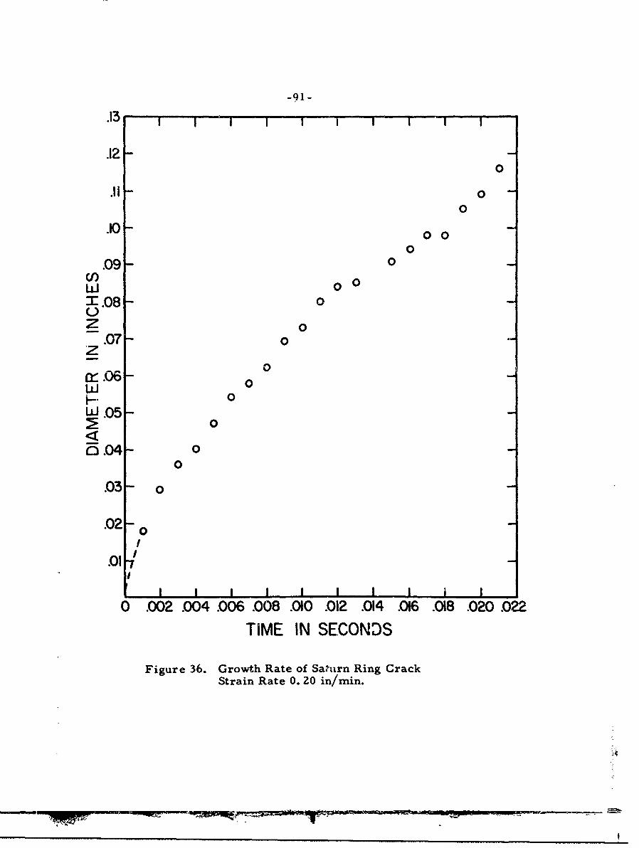
-91-
.13 1 I I 1 I '
.120
.11 00
.10 0 00
.09 0(1)0ILl 0
-E.08 00z 0
.07- 0z
n, .06 - 0
IL-I .05H 00
0.04 00
.03 o
.02 0
I
.01'
I I I I I I I0 .002 .004 .006 .008 .010 .012 .014 .016 .018 .020 .022
TIME IN SECONDS
Figure 36. Growth Rate of Saturn Ring CrackStrain Rate 0. ZO in/min.

-92-
under which the actual filming was performed, the entire propagation
history could not be recorded; especially the short-time regime.
This is indicated in the figure by a dotted line as an extrapolation
back to the original flaw size.
It appears then in retrospect from evidence studied a posteri-
ori and coupled with other evidence acquired before and during frac-
ture that:
1) Fracture nucleates probably from a point of weakness in
the material.f: 2) The early phase of fracture is a static one that can be
approximated as crack propagation at virtually zero velocity, where
bonds are broken slowly.
3) After reaching a critical size the crack will rapidly accel-
erate and the remaining surface changes from a rough and coarse
one to a mirror-like or glassy one.
4) This critical stress is almost three t-im-es the uniaxial
strength.
5) The acceleration period is very short and is followed by
a steady state situation where the fracture surface propagates at a
constant velocity until it intersects the boundaries.
6) It then propagates as a very blunt crack along a trajectory
that takes it perpendicular to the plane of the maximum principal
stress of the distorted field.
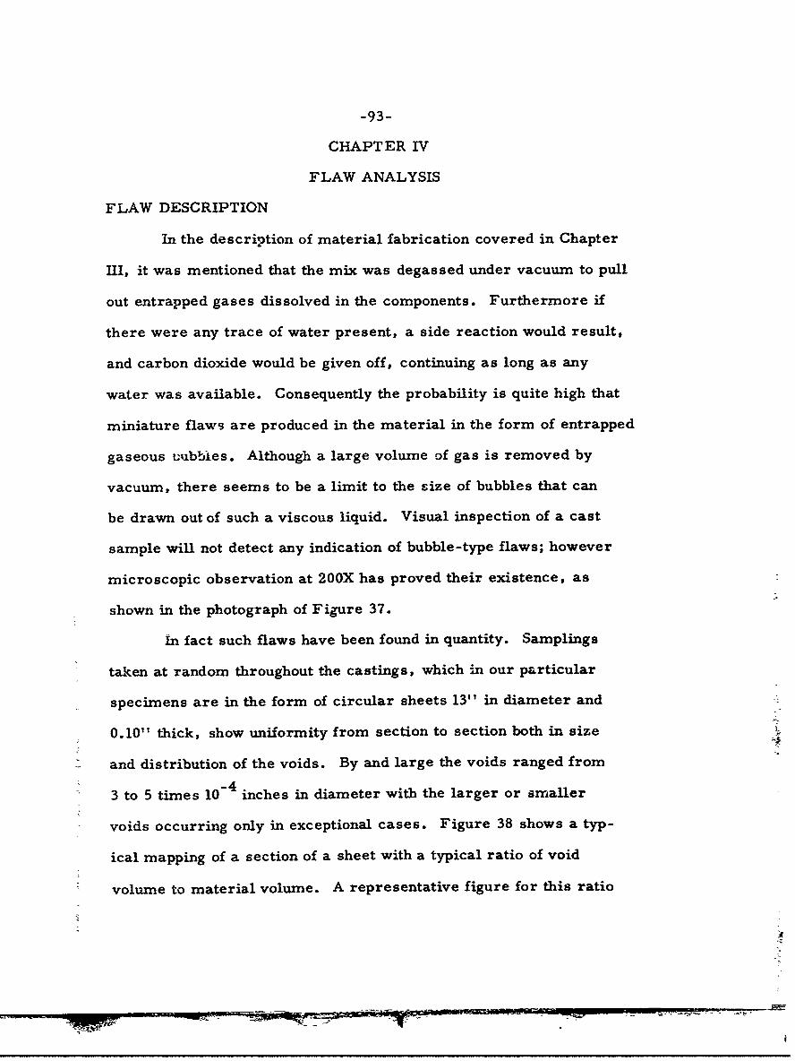
-93-
CHAPTER IV
FLAW ANALYSIS
FLAW DESCRIPTION
In the description of material fabrication covered in Chapter
III, it was mentioned that the mix was degassed under vacuum to pull
out entrapped gases dissolved in the components. Furthermore if
there were any trace of water present, a side reaction would result,
and carbon dioxide would be given off, continuing as long as any
water was available. Consequently the probability is quite high that
miniature flaws are produced in the material in the form of entrapped
gaseous =ubbles. Although a large volume of gas is removed by
vacuum, there seems to be a limit to the size of bubbles that can
be drawn out of such a viscous liquid. Visual inspection of a cast
sample will not detect any indication of bubble-type flaws; however
microscopic observation at 200X has proved their existence, as
shown in the photograph of Figure 37.
in fact such flaws have been found in quantity. Samplings
taken at random throughout the castings, which in our particular
specimens are in the form of circular sheets 13" in diameter and
0.10" thick, show uniformity from section to section both in size
and distribution of the voids. By and large the voids ranged from
-43 to 5 times 10 inches in diameter with the larger or smaller
voids occurring only in exceptional cases. Figure 38 shows a typ-
ical mapping of a section of a sheet with a typical ratio of void
volume to material volume. A representative figure for this ratio
M noA
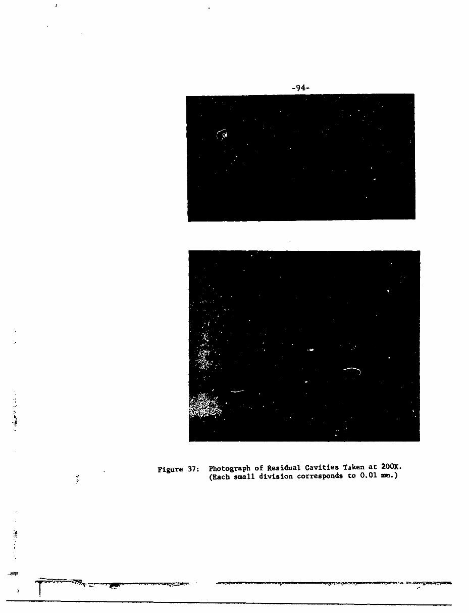
-94-
Io
Figure 37: Photograph of Residual Cavities Taken at 200X.(Each small division corresponds to 0.01 wi.)
-RA70'F, " M nwI
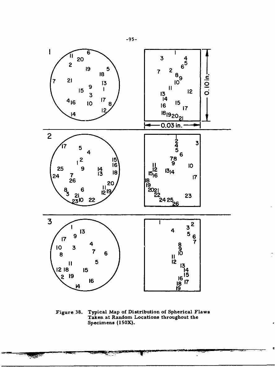
-95-
3 1 64
187 2, 8
71819221
0--.03,in.---
54 56
825 9 14 SI 013 13
\ 6 o/ 1 2 1II I
21 2223
10 104
512 13
26 18 17199
Figure 38. Typical Map of Distribution of Spherical FlawsTaken at Random Locations throughout theSpecimens (I 50X).
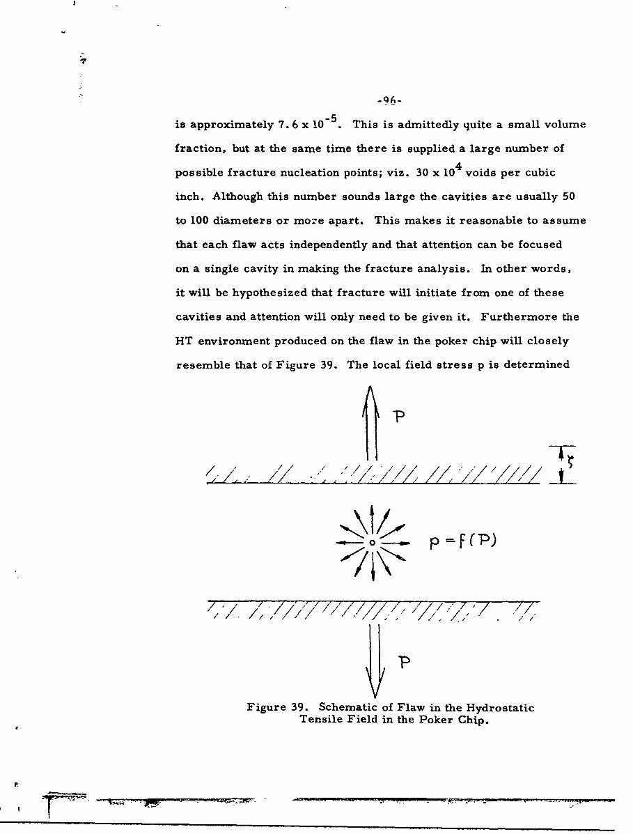
I5 S~-96-
is approximately 7. 6 x 10-. This is admittedly quite a small volume
fraction, but at the same time there is supplied a large number of
possible fracture nucleation points; viz. 30 x 104 voids per cubic
inch. Although this number sounds large the cavities are usually 50
to 100 diameters or more apart. This makes it reasonable to assume
that each flaw acts independently and that attention can be focused
on a single cavity in making the fracture analysis. In other words,
it will be hypothesized that fracture will initiate from one of these
cavities and attention will only need to be given it. Furthermore the
HT environment produced on the flaw in the poker chip will closely
resemble that of Figure 39. The local field stress p is determined
" ,'.- / ," . /, / / / /. .' -//•/ ,. fi/ // /
X/
Figure 39. Schematic of Flaw in the HydrostaticTensile Field in the Poker Chip.
-97-
from the applied load P or boundary displacement 6 through Figure 8.
Then since the cavity is small compared to the specimen thickness,
an analysis can be made considering the flaw to be alone in an infinite
hydrostatic field, and the test will closely duplicate the theoretical
assumptions and boundary conditions.
The approach to be followed will be to consider the transfer
of energy for the cavity region during the fracture process. From
this a critical value of the hydrostatic pressure will be predicted in
terms of pertinent material and geometric parameters, indicating
the point of rupture of the spherical flaw. However this will require
some extensions of the classical concepts in order to deal with this
particular geometry, stress field, etc., and a genwral discussion of
the energetics of fracture is in order.
ENERGY CRITERIA FOR ELASTIC FRACTURE
To a novice in the field it appears that there is great need
for elucidation of the basic principles upon which fracture energetics
are built; so that extensions to other geometries, other stress
fields, and other materials will be clear. Since this will have to be
done in the instance of the spherical cavity, let us review a few fun-
damentals.
Conservation of Energy
Beginning with the First Law of Thermodynamics as applied
to a general fracture process (65) it is possible to arrive at Grif-
fith's classical results, (66) which were originally obtained in quite
a different manner. The recoverable strain energy U1 , representing
-98-
the strain energy before fracture, plus the work done by the surface
tractions during fracture, 6W, must, from the Conservation Law,
equal the strain energy after fracture U2 , plus the energy dissipated
in forming new surface 6S.
U1 + 6W =U 2 + 6S (4.1)
or forming an incremental equation
AU - 6W + 6S = 0 (4.2)
Differential Form
It is convenient for computation and for later comparisons
to cast the energy equation into a differential form. This will be
accomplished by dividing the equation by an increment of crack
length and taking the limit as the change in crack length approaches
zero. Implicit within this operation is the assumption that each
term in the equation can be written as a continuous function of crack
length, which can only be done if the flaw hypothesis is made.
This results from the fact that the fracture point of a specimen
with a residual crack is actually the point of initiation of the prop-
agation phase, and the energy terms can be represented as contin-
uous functions of crack length. On the other hand, if there is no
microscopic flaw and fracture originates at a sub-continuum level,
then the energy terms are not continuous functions of crack length,
and the incremental equations must be used, The differential form
of the conservation law for a fixed force boundary condition be-
comes#
jrS

-99-
dU _F 6 dA 0 (4.3)dA FdA
where F =Applied force at the boundary
6 =Displacement of the boundary
y = Surface energy density
A =New surface created during fractures
E.,.ER GY FUNCTIONALS
Consider now certain energy functionals which have been used
in fracture analysis. The Potential Energy Functional can be con-
sidered as a starting point for Griffith's (66) discussion of fracture.
In attempting to translate his discussion into mathematical terms
we obtain,
V U - P+S (4.4)
where U = Strain energy
P = Potential of the boundary load computedwhile the load is held constant
S = Surface energy
C"= 6U - 6P + 6S (4.5)
By a careful comparison of expression (4.2) and (4.5) and the physi-
cal processes which they describe, (30) it can be shown that 6P =
6W. This is the crux of an argument that can be used to establish
what Griffith assumed for the fracture criterion, i.e.,
V O- + dc= 0 (4.6)[ YCU- 0-C dc]
-100-
By a comparison with the energy equation (4.3), it is apparent that
they are identical. This is a significant result, for it establishes*
that fracture predictions for fixed grip loading made on this basis
of the adjusted potential energy being a rn'uimum, are the same as
obtained from energy conservation. At this point it is difficult to
ascertain just why a minimization of y should predict fracture, but
a later examination of the stability aspects of the problem will
clarify this point.
Extended Complementary Energy. If a similar comparison
is made between the extended potential energy of equation (4.4) for
fixed grip loading and the energy balance made for the same condi-
tions, it can be demonstrated that the two do not coincide and that
the two conditions are not the same. It is therefore concluded that
the extended potential energy is not the correct functional for fixed
grip loading. However an analogy can be made between the types of
loading and the correct functional, for in the case of fixed force
loading, where the force is held constant and the displacements
are varied, it was found that the potential energy was the proper
functional; therefore it would appear appropriate that for the fixed
grip condition where the displacements are held constant and the
forces are varying that complementary energy (49) should be con-
sidered.
It turns out that this is true. A direct comparison can be
Griffith did not specify the boundary conditions with which he
worked, but it can be deduced that it had to be fixed force.
'W T -7

-101-
madue and a minimization oi an altered form of the complementary
energy functional.
V =U-Q+S (4.7)
where Q = fZF_1 6i1 &
26 = Portion of the surface where displacementsare specified
dor = Differential surface element
coincides with the energy equation (4.3). At this point the physical
reason why 6V = 0 predicts fracture is obscure, but it will be ex-
plained by considering the stability of the crack.
STABILITY
By means of the conservation law 6f energy, it has been pos-
sible to establish a necessary condition for fracture, since it is
necessary that energy be conserved for the phenomenon to occur.
Now it is of interest to inquire into the stability of the crack; whether
it be in stable, neutral, or unstable equilibrium. Classically it is
the second variation that provides information on stability, but this
is not necessarily always the case. Sometimes the very nature of
the problem will cause the first or possibly the first and second
variations to vanish identically. (67) In fact, there is no limit to
the number of variations that can vanish and consequentl/ it is not
a set principle as to which variation controls stability. This turns
out to be the case in the general fracture problem that we are cur-
rently investigating. In order to see this, let us take a closer look
'4 *"own WE
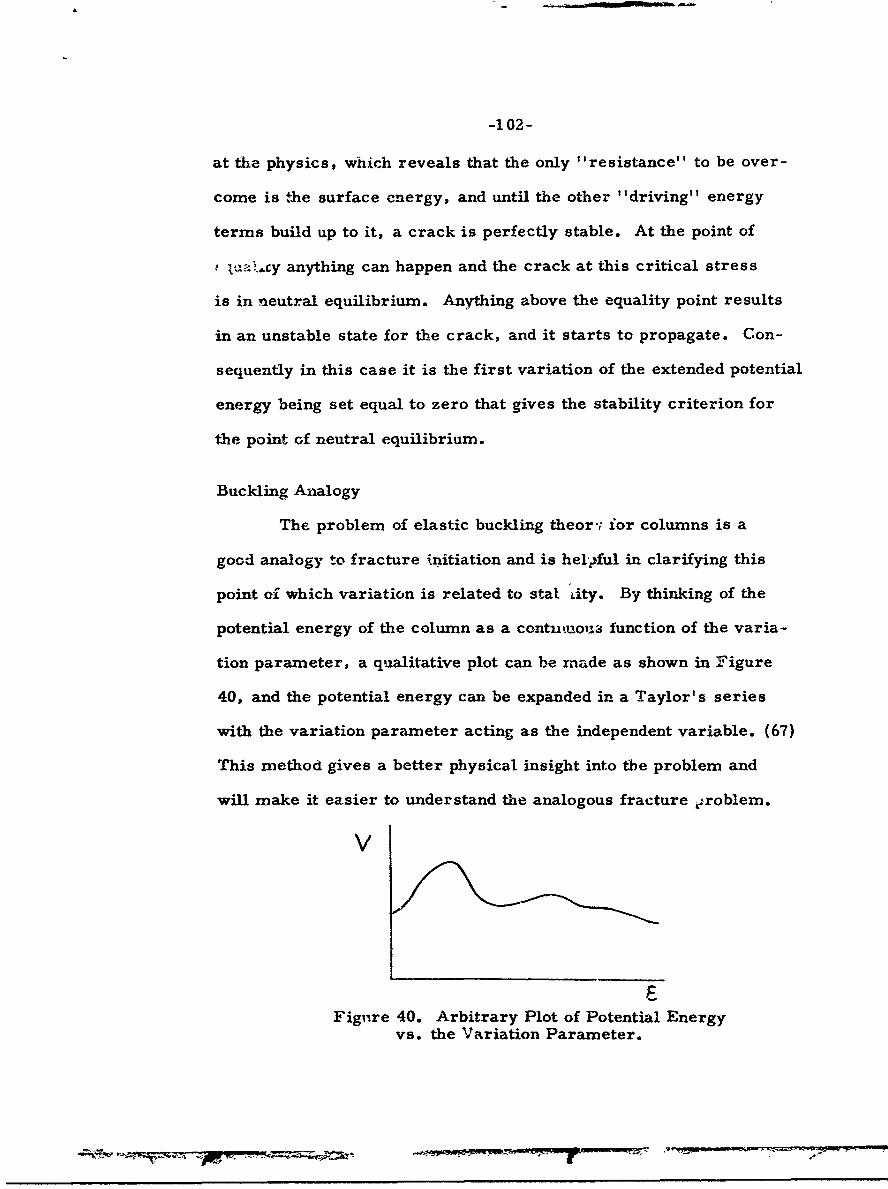
-102-
at the physics, which reveals that the only "resistance" to be over-
come is the surface energy, and until the other "driving" energy
terms build up to it, a crack is perfectly stable. At the point of
•txa>..cy anything can happen and the crack at this critical stress
is in neutral equilibrium. Anything above the equality point results
in an unstable state for the crack, and it starts to propagate. Con-
sequently in this case it is the first variation of the extended potential
energy being set equal to zero that gives the stability criterion for
the point of neutral equilibrium.
Buckling Analogy
The problem of elastic buckling theor i ior columns is a
good analogy to fracture initiation and is hel',ful in clarifying this
point of which variation is related to stal Lity. By thinking of the
potential energy of the column as a contntuoa function of the varia-
tion parameter, a qualitative plot can be made as shown in Figure
40, and the potential energy can be expanded in a Taylor's series
with the variation parameter acting as the independent variable. (67)
This method gives a better physical insight into the problem and
will make it easier to understand the analogous fracture ýroblem.
V
Fignre 40. Arbitrary Plot of Potential Energyvs. the Variation Parameter.
-103-
A Taylor's series expansion is readily written as
2V = V(0) + V'(O)E + V"(0) C+ ... (4.8a)
However, by definition of the variation operator (68)
AV = 6V+ 62 V + 63+ ... (4.8b)
Thus if we are at an equilibrium point, the first variation vanishes
and the sign of AV ia determined by the second variation, or in other
words, the second variation gives information about stability. The
one additional facet that affects the column buckling i3 that AV is
computed around a loading position when buckling is imminent;
therefore AV becomes a second order incremental change on top
of the AV generated by loading from the natural state to th : point
of buckling. Consequently, if the potential energy is used, the first
variation about the loaded state corresponds to a second variation
about the initial state, so that the first variation for column buckling
actually becomes equivalent to a second variation and gives the
point of instability.
A similar set of circumstances prevails in the instance of
imminent fracture, where we are using the extended potential
energy. For, as in the case of buckling, the first variation about
the point where fracture is imminent corresponds to a second var-
iation a ,out the natural state, and it is therefore the first variation
that gives the information about crack stability. This can also be
seen from the fact that the critical point using the extended potential
energy was actually based upon the first law of thermodynamics,
which implies that a state of equilibrium prevails. Interpreted in
the light of a series expansion for V. this would mean that the first
variation, which is concerned with equilibrium, is automatically
satisfied. Thus in the expansion the first term that appears is
actually the second variation and is the one that is of interest when
seeking information about stability. From this it is seen that for
fracture prediction we are not dealing with equilibrium principles
as Griffith discussed but stability, and now it is clear why the
vanishing of the first derivative of the adjusted potential energy
is the appropriate fracture condition.
In summary it may be stated that the conservation of energy
provides a necessary condition for fracture as well as a basis upon
which the potential energy can be extended; furthermore, the value
at which the first variation of the new functional vanishes is the
point of neutral equilibrium, demonstrating that the crack will run
at this point, and this constitutes a type of sufficiency condition for
fracture. Therefore the critical values predicted by this analysis
are necessary and sufficient conditions for fracture within the limit
of the degree to which the physics are modeled by the mathematics.
ENERGY FRACTURE ANALYSIS - INFINITESIMAL THEORY
We return now to consider the growth and eventual rupture
of a spherical cavity in an infinite medium subjected to HT at infin-
ity. Based upon the findings described previously in relation to the
existence, location and distribution of spherical flaws, a boundary
value problem formulated for this geometry would be expected to
- ••~'-' =r-•• •
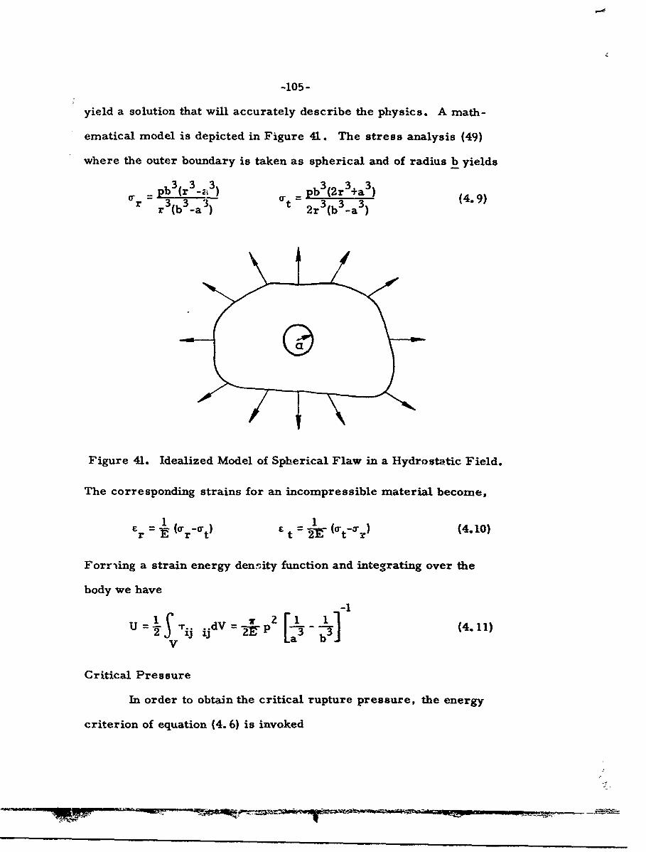
-105-
yield a solution that will accurately describe the physics. A math-
ematical model is depicted in Figure 41. The stress analysis (49)
where the outer boundary is taken as spherical and of radius b yields
r 3pb 3 (r3-•a pb 3(2r 3+a3 (4.9)r r 3(b3_a3) 2r3(b3-a3)
Figure 41. Idealized Model of Spherical Flaw in a Hydrostatic Field.
The corresponding strains for an incompressible material become,
r1 rt t = t-r) (4.10)
Forriing a strain energy density function and integrating over the
body we have-1
U b-dV 5 d3 (4.11)V
Critical Pressure
In order to obtain the critical rupture pressure, the energy
criterion of equation (4.6) is invoked
ITI14 W-

-106-
S(U-S) = 0 (4.12)
where for a linearly elastic material P = -2U. (69) S represents the
energy required to create unit surface, and a is a measure of the
flaw growth. In this instance when b >> a, equation (4.12) becomes
.a [- p 2 a 3 -4va2Y] = 0 (4.13)
which yields a critical pressure of
Pc = ( (4.14)
Flaw Size Dependency
This gives the typical inverse square root dependency of
critical rupture stress on initial flaw radius. In fact, the defining
equation of (4.13) varies only slightly for the entire spectrum of
flaw geometries. Sneddon (70) and Sack (71) obtained the inverse
square root dependency for I 'penny-shaped'" cracks in hydrostatic
fields, which is very similar to the Griffith (66,72) result for the
line crack in a two-dimensional sheet.
A summary table shows the quantitative similarity for rep-
resentative geometries (73)
Geometry Sheet with Cylindrical Penny-shaped Sphericalline crack cavity crack cavity(Griffith) (Sneddon)
Critical ai_.5 4 ]ýFW JEj_Stress Iza 2a 3a "3 a
WilliamfJ (73) has discussed this similarity and uses it to investigate
the more complicated phenomenon of viscoelastic fracture.
T 17- 0- 7_________________
A-
-107-
Mode of Propagation
It should be noted that the analysis inherently assumes a
radial mode of propagation for the fracture surface; i.e., that the
flaw grows spherically in a manner similar to ablation. This may
place a limitation on the information gained, but a similar situation
arises for the "penny-shaped" crack, which also is confined to
propagate radially in a planar mode. Only experimentation can
provide the means for evaluating these assumptions and determining
what portion or portions of the fracture process can be analyzed
by them.
ENERGY FRACTURE ANALYSIS - EFFECT OF FINITE DEFORMA-
TION
The spherical symmetry in this problem makes it possible
to extend the infinitesimal deformation fracture analysis to include
effects of finite deformations. This is seldom possible, although
Gent and Lindley (24) did use the model of a spherical cavity in an
infinite medium and investigated the strains at the cavity using a
maximum strain criterion. S&:hapery and Williams (74) used a non-
linear theory for the same problem and coupled it with an energy
criterion to predict fracture. This is a particularly interesting
approach for polymeric materials where large strains are the rule;
furthermore, it provides an opportunity to see how large strains
affect the inverse square root dependency of initial flaw size.
Finite Strain Effects
The presence of deformations exceeding the limits of infini-
* tesimal theory produces many ramifications in the mechanics of the
-108-
energy analysis: First, the matter of loading requires a more care-
ful definition to fit the actual conditions both experimentally and
theoretically, for with finite strains the change in area of the bound-
ing surfaces is accounted for and there becomes a distinction between
fixed force and fixed stress conditions. This difference will manifest
itself in almost every quantity previously calculated and will affect
the outcome of the conclusions drawn on the basis of the infinitesimal
theory.
Second, this same matter of the differences between the de-
formed and the undeformed area produces questions about the manner
in which surface energy is handled in the governing expressions.
Normally in the-.e computations, a surface energy is computed as if
it were a variabie of state; i.e., as if the existing surface possessed
a given surface energy as opposed to only speaking of changes in the
surface, or energy required to create surface. The actual compu-
tation is then made by differentiating this quantity with respect to
the crack length. However add.tional consideration must be given
when the surface of interest is significantly altered by deformation
before fracture occurs, i.e., the original surface changes in area
but does not rupture. This deformation is accounted for in the stress
analysis of the body and in the energy expressions, but the correct
nm. nner in which it influences the surface energy may be debatable.
Third, the classical potential energy theorem has been
shown to apply regardless of the magnitude of strain. For example,
Green and Zerna (75) derived the theorem for large strains, and
the form of the expression is found to be identical with the linear
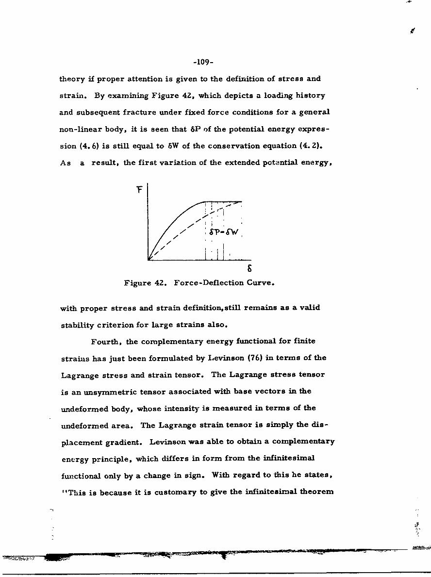
-109-
theory if proper attention is given to the definition of stress and
strain. By examining Figure 42, which depicts a loading history
and subsequent fracture under fixed force conditions for a general
non-linear body, it is seen that 6P of the potential energy expres-
sion (4.6) is still equal to 6W of the conservation equation (4. 2).
As a result, the first variation of the extended potential energy,
Figure 42. Force-Deflection Curve.
with proper stress and strain definition, still remains as a valid
stability criterion for large strains also.
Fourth, the complementary energy functional for finite
strains has just been formulated by Levinson (76) in terms of the
Lagrange stress and strain tensor. The Lagrange stress tensor
is an unsymmetric tensor associated with base vectors in the
undeformed body, whose intensity is measured in terms of the
undeformed area. The Lagrange strain tensor is simply the dis-
placement gradient. Levinson was able to obtain a complementary
energy principle, which differs in form from the infinitesimal
fimctional only by a change in sign. With regard to this he states,
"This is because it is customary to give the infinitesimal theorem
MS- -- . ~
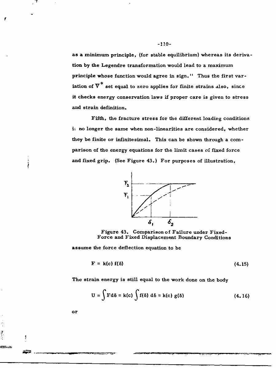
r"
-!!0-
as a minimum principle, (for stable equilibrium) whereas its deriva-
tion by the Legendre transformation would lead to a maximum
principle whose function would agree in sign." Thus the first var-
iation of V set equal to zero applies for finite strains also, since
it checks energy conservation laws if proper care is given to stress
and strain definition.
Fifth, the fracture stress for the different loading conditions
i,. no longer the same when non-linearities are considered, whether
they be finite or infinitesimal. This can be shown through a com-
parison of the energy equations for the limit cases cof fixed force
and fixed grip. (See Figure 43.) For purposes of illustration,
T,
S6S 2
Figure 43. Comparison of Failure under Fixed-Force and Fixed Displacement Boundary Conditions
assume the force deflection equation to be
F = k(c) f(6) (4.15)
The strain energy is still equal to the work done on the body
U =Fd6 = k(c) Of(N) d6 k(c) g(M) (4.16)
or
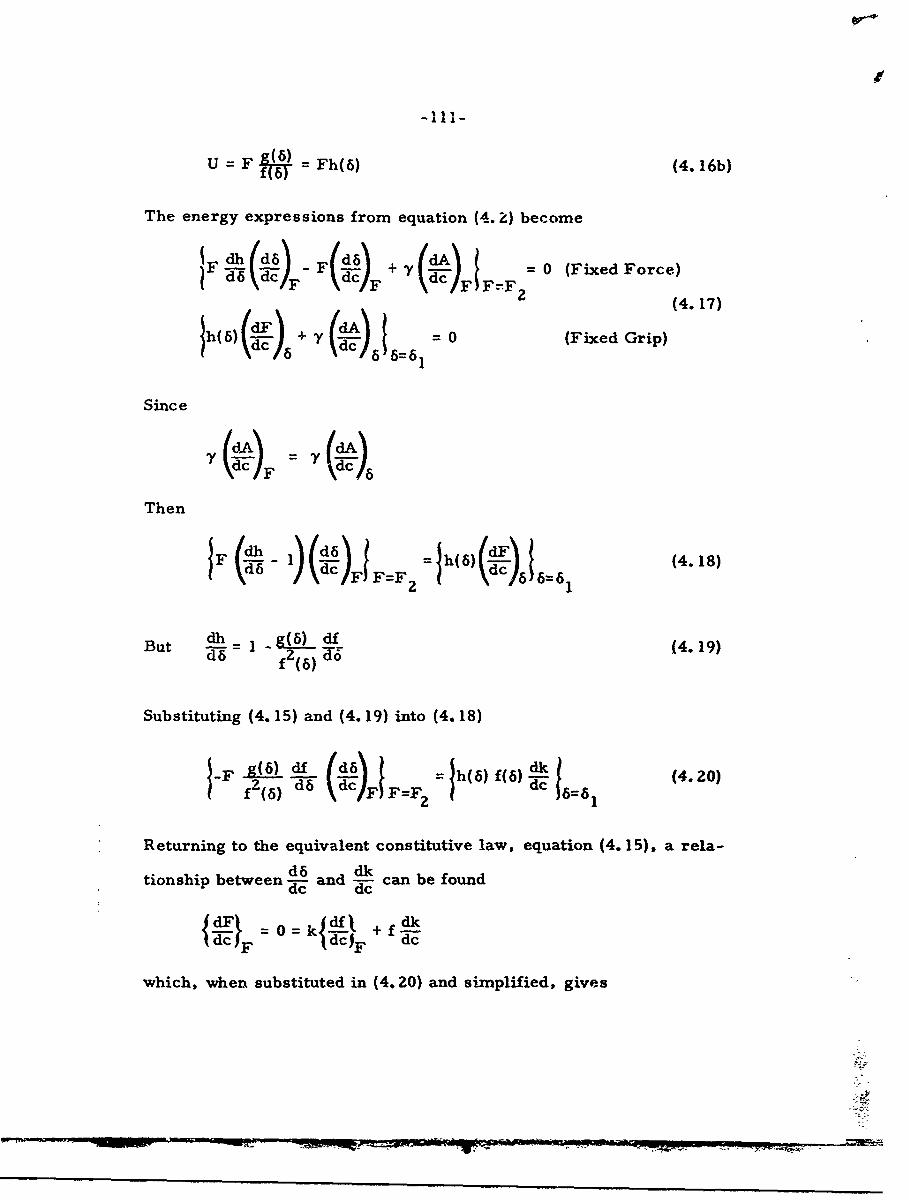
(
U = F = Fh(6) (4.16b)
The energy expressions from equation (4. k) become
~F ý(ýd-) -F(ýdC)F +~ -y(ý)F I F= 0 (Fixed Force)17
1h(6) + 'Y =0 (Fixed Grip)6 =61
Since
( ddA
Then
1F(6 ))( ); 4h(6)(~ (4.18)I] F (dc) 1.6. 6d1
But dh - Ig(6) df (4.19)d-6 fZ2( 6) TIE
Substituting (4. 15) and (4. 19) into (4.18)
9(6)df () F=F h(6) f(6) =1 (4.20)
Returning to the equivalent constitutive law, equation (4. 15). a rela-
tionship between ý-- and 4 can be founddc dc
0 =0=kj + fA
dc}F{ dc)F dc
which, when substituted in (4. 20) and simplified, gives
NWI% I
-ll2-
h(F 61 F (4.21)
The conclusion which follows is that in general for non-linear
systems, the fractuare stress depends upon the form of the stress-
strain law as well as the boundary loads, and the specific cases must
be analyzed. For instance, if f(6) = .1/n the critical stresses coin-
cide, but the nature of the system must always be examined to make
certain. This could possibly explain some discrepancies in poly-
meric fracture data, for in the instance of typical material repre-
sentations such as Neo-Hookean or Mooney-Rivlin, the critical loads
will not coincide because of the form of the constitutive law. (77)
CRITICAL FRACTURE POINT
The critical fracture stress will now be computed for both a
Neo-Hookean (NH) and a Mooney-Rivlin (MR) material to provide
not only a comparison between the two non-linear stress-strain
laws, but also with the infinitesimal theory. The strain energy
funciun for both can b represented by
W - 1+(I-3) + (l-f) %I - 3 13 = 1 (4.22)
where f = 1 gives NH, and 0 - f < 1 is MR. Following Levinson (78)
the relation between the hydrostatic tensile pressure, p, applied at
infinity and the stretch ratios of the inner boundary a and outer
boundary b is
(4. 23)
-113-
From incompressibility
b3- a03= b 3 -a 3 (4. 24)
where a 0 , b0 denote undeformed measures of the radii.
This can be rewritten as
a3 (X3 -)=b33 (.50a 0(X )b(Xjý*l 4.u
or1/
1 + .0 (;L _ 1(4.26)'Lb = I -bo/ Y a"14.)
However for an infinite medium a/b0 < <1; furthermore, a /b 0 =Xa
a << 1. From the binomial expansion
b0
n +n () a *" (4.27)
Substituting (4.27) into (4.23) the pressure relation simplifies to
E•f 4 1-E 2Xa+ 1 (4.28)T a
Strain Energy. As was previously discussed, the altered or
extended form of the potential energy functional can also be used for
finite deformations. Of course the boundary conditions remain as
constant pressure during fracture and the potential of the surface
forces is no longer twice the strain energy as in the linear theory.
AU three energy terms must now be individually computed and in-
serted into the governing energy equation (4. 6)
a [ u-p+ s =o (4. 29)8a0
-114-
where U = Strain Energy
P = Potential of Surface Forces
S = Surface Energy
The strain energy is computed through the defining integral
b 3
U =3 4spb db =3 41rpb0 X-ýdXb (4.30)
b1
Using (4.27) to express the integral in terms of the extension ratio
at the flaw cavity, (4.30) becomes
U 4wb (a ( dka (4.31)
1
where the fact that a 0 /b 0 < I has been used to simplify the expres-
sion. Substituting the expression for p, equation (4.28), and inte-
grating
4
= aEI-f)X+ (7+-21 X3 2- ( Of) + _ 4.32)a
Potential of Surface Forces. This is a much simpier term
to compute due to the fact that p is now held constant.
P = 4zpb0 (b-b 0 ) = 4 rpb31Xb-l) (4.33)
Using (4.27) once again
P =.Ipa0 a( -1 (4.34)
Surface Energy. One of the new facets of the problem alluded
to previously is encountered at this point. Before rupturing, the
-115-
cavity surface may undergo a large change in surface area, which
would be considered as a stretching of the molecular structure, with
all input energy remaining recoverable. At the critical point, energy
will be dia3sipated by the formation of new surface, and although the
cavity is deformed considerably, the surface energy density should
be referred to the cavity surface before deformation. The reason
being that y, the surface energy density, is an artifice that relates
molecular activity to continuum activity. Consequently it is the
number of molecules present on the surface that is of concern in
computing fracture energies. This remains constant during the
deformation and therefore
2S = 40ray (4.35)
CRITICALITY EQUATION
Substituting equations (4.32), (4.34) and (4.35) iato the
energy equation of (4.29) and performing the differentiation, with
p held constant, we obtain
X--2 6 +kXý + 2). +-f 0 (4.36)a 1-f a 1-f a a 1f
This expresses the critical condition for fracture in terms of the
stretch ratio at the cavity and a material parameter k =
The simplest case is for the NH material when f = 1, then the criti-
cal condition is (41)
A6 3 4 1a-(j+k) (a + 14,37)
A check of this polynomial reveals that there is only one
P" -"P

-116-
positive, real root greater than one, so no complicated interpreta-
tions arise. Of course once the critical extension ratio is known,
the critical pressure can be computed from equation (4.28), and for
completeness, the expression for the tangential hoop stress is
given.
It= f+ •X ] (I[x --f] (4.38)
a
Comparative Results. All of these quantities have been
plotted collectively for comparison in Figures 44 - 46. There is
a noticeable variation in almost every quantity, as for instance
the ultimate extension of the cavity surface for NH bodies is in-6T
creased considerably over MR b.-dies for log r- greater than0
0.50, while the reverse relation holds for the hydrostatic field
stress p. In this case, p for the NH body approaches an asymptote5E
of 5, while MR exhibits behavior characteristic of the infinitesi-
mal theory and as a result these two curves diverge rapidly. How-
ever for both NH and MR the inverse square root dependency on
a0 is reduced by considering finite strains. In spite of this reduc-
tion, there still remains a strong influence of a 0 on pc.
The validity of these predicted fracture levels can only be
ascertained by experiment. In this connection, a method was
conceived for inserting artificial flaws of varying sizes into the
polker-chip specimen and subjecting them to HT. Details of these
results, to be described subsequently, shed light oI& the fracture
behavior of spherical cavities and provide further information for
evaluating the flaw analysis.
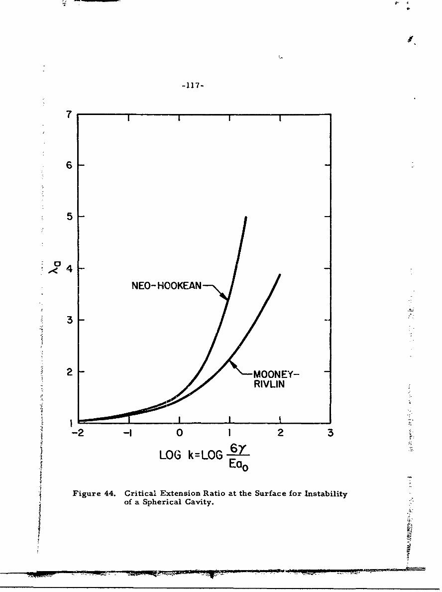
-117-
7
6
4
NEO- HOOKEAN
3
2 -MOONEY-RIVLIN
-2 -I0 I2 3
LOG k=LOG EaE0
Figure 44. Critical Extension Ratio at the Surface for Instabilityof a Spherical Cavity.
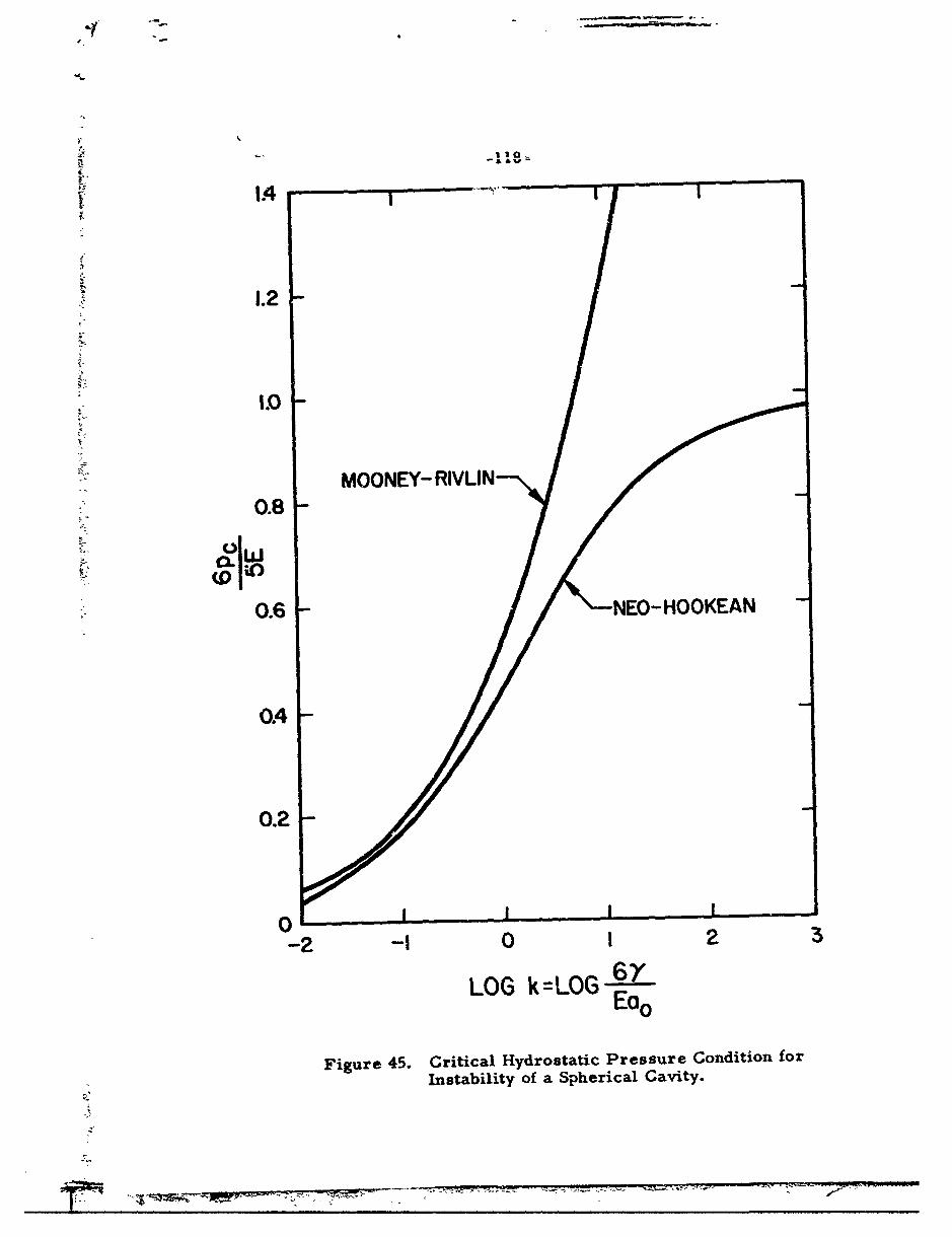
aI
1.2
MOONEY- RIVLIN0.8
i '~
0.6 NEO-HOOKEAN
0.4-
0.2
0-2 -I 0 1 2 3
LOG k=LOG 6a'Eoo
Figure 45. Critical Hydrostatic Pressure Condition forInstability of a Spherical Cavity.
Tý T.' 17
7:7 4
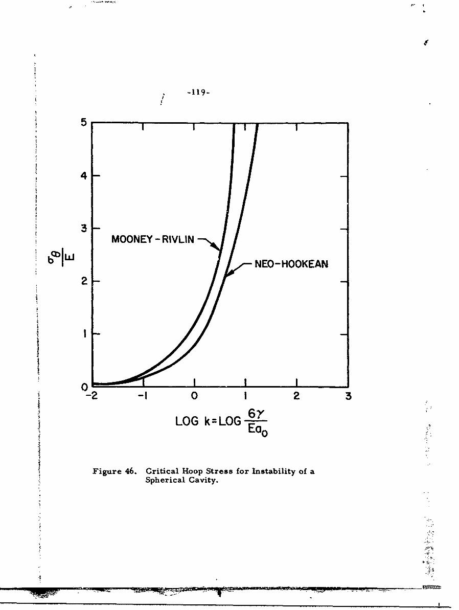
-119-
i 5
4
13
MOONEY - RIVLIN
bI NEO-HOOKEAN
0
-2 -I 0 I 2 3S~6Y
LOG k=LOGE--Ea0S0 0 •0
Figure 46. Critical Hoop Stress for Instability of aSpherical Cavity.
......

CHAPTER V
ARTIFICIAL FLAWS
As a means of further assessing the theoretical treatment,
k as well as serving as a vehicle for the study of flaw behavior, a
number of poker-chip specimens were prepared with a dominant
J central flaw in the form of an air bubble. In order for experiments
for such a specimen to be meaningful, the cavities must be inserted
without disturbing the normal manufacturing operations of the
standard material. It will be recalled that the standard manufac-
turing operat.on consisted of mixing together the two components,
pre-polymer and catalyst, under an inex atmosphere of nitrogen.
The mix is then transferred to a preheated mold through piping that
enables the mold to be filled while in the oven. The specimen is
then cured at 150 0 C for two hours. The bubbles were inserted into
the material without interrupting this operation by constructing a
mold with a glass front as shown in Figure 47.
N'eedle hole loss Plsate
S• fill H ole
Figure 47. Mold Asser-Aly
iN.

-121-
The spacer ring was fitted with a hole to admit a long hypo-
dermic needle, which was of sufficient length to reach from a syringe
outside of the oven to the inner parts of the mold. In the apparatus
used, the needle was two feet long. The two components were mixed
and preheated as before, and the preheated glass front mold was
filled while in the oven in the usual manner. The polyme,'•zation
and cross-linking process begin to take place immediately upon
mixing of the two components; however, there is a pot life during
which the material will flow even though it is becoming more viscous
with time. It is while the polymer is still in this liquid state that
the hypodermic needle is inserted into the mold and a bubble blown
from outside the oven. The needle is withdrawn before the liquid
has become solid enough to retain any memory of its presence.
The mold was mounted on a shaft capable of rotation by an electric
motor controlled from the outside of the oven. In this way, the
location of the bubble in the mold could be controlled, as it had a
tendency to rise during the early stages before the polymer became
solid. The complete arrangement is shown in Figure 48.
Mold
Figure 48. Schematic of Apparatuzz used for Inserting Artificial Flaws
-122-
Following this oper , the specimen was cured in the standard
manner at 150°C for two hox:rs, and then removed from the mold
and stored in a dry box until used.
OBSERVATIONS
The specimen was mounted between lucite grips as before
with the dominant flaw located in the center. Direct visual obser-
vation of the growth of the flaw under load was made by means of
a portable microscope from which several interesting things were
learned: 1) Deformations at the surface of the cavity were defi-
nitely finite, with strains ranging up to 150 percent. This is quite
unusual since the maximum strain in uniaxial tension attains values
of only 35 to 40 percent, but it appears that the necessary energy
condition for fracture is not met in this configuration until a sig-
nificantly larger strain. It should be emphasized, in light of the
stress axis theorem discussed previously, that these are the local
strains around the cavity and not the global strains measured at
the boundaries, which were still small in this test. 2) Fracture
levels were not affected by the presence of the dominant flaw but
were unchanged from those of the regular specimens. 3) Fracture
did not occur at the artificial flaw but elsewhere in the specimen,
sometimes close and sometimes distant from the bubble. Even in
the few cases where multiple artificial flaws were inserted in the
same specimen, fracture still occurred in the field rather than on
the surface of one of these cavities. 4) None of the cracks after
nucleating elsewhere ever propagated into or through a bubble; all
-123-
bubbles remained intact and could be seen unruptured after the spec-
imen was completely severed into two pieces. This led to the exam-
i ination of fracture of the material in other geometries to determine
if the cracks had propagated through any of the residual bubbles
regardless of the initial size, but no evidence could be found. A
behavior of this nature was noted by Schwarzl and Staverman (79)
in Plexiglas but in this instance it was concluded that the bubbles
are not a mechanism of propagation; in fact, almost the opposite is
S true. The propagating surface seems to either stop or go around
such a discontinuity in the material.
It should be noted in the interpretation of these results that
the dominant flaw was still surrounded by a matrix of the residual
flaws, since the material was produced in a standard way. The
i large cavity was not alone in the field, and it is felt that a signif-
icant difference in behavior would have been noted had it been alone.
Since there still remained the distribution of tiny bubbles, invisible
to the naked eye, the experiments are taken as evidence of the
validity of a so-called Saturn-ring theory of crack propagation.
SATURN-RING CRACK
Assuming as before that the flaws are dispersed widelyIS
enough not to interfere with each other or cause disturbances in
the hydrostatic stress field, we will focus our attention on a single
cavity in an infinite field that will eventually trigger the fracture.
Let us visualize a reasonable physical mechanism by which fracture
can occur by picturing the cavity as it grows under the action of
I the hydrostatic tension. As the pressure is increased, the cavity
7- - - =
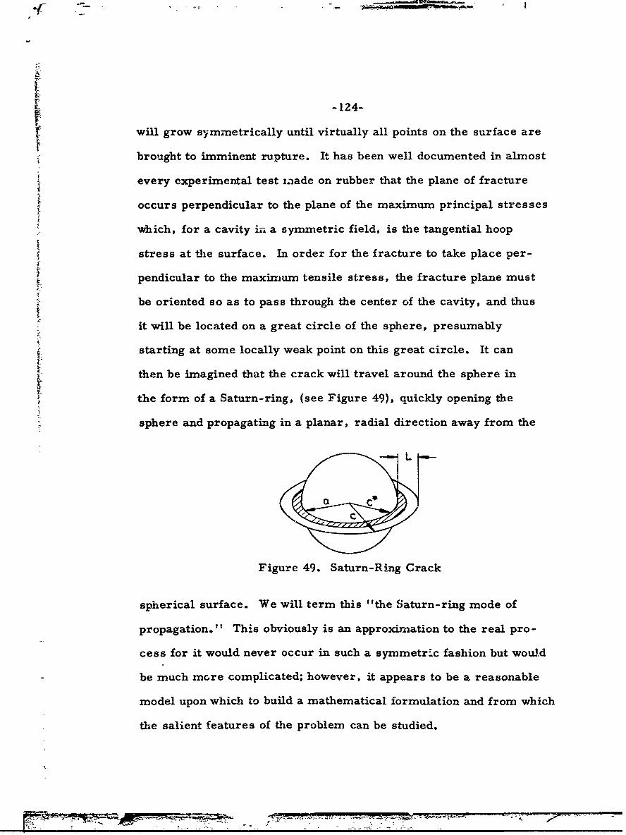
-124-
will grow symmetrically until virtually all points on the surface are
brought to imminent rupture. It has been well documented in almost
every experimental test inade on rubber that the plane of fracture
occurs perpendicular to the plane of the maximum principal stresses
which, for a cavity in a symmetric field, is the tangential hoop
stress at the surface. In order for the fracture to take place per-
pendicular to the maximum tensile stress, the fracture plane must
be oriented so as to pass through the center of the cavity, and thus
it will be located on a great circle of the sphere, presumably
starting at some locally weak point on this great circle. It can
then be imagined that the crack will travel around the sphere in
zi the form of a Saturn-ring, (see Figure 49), quickly opening the
"sphere and propagating in a planar, radial direction away from the
Figure 49. Saturn-Ring Crack
spherical surface. We will term this "the Saturn-ring mode of
propagation." This obviously is an approximation to the real pro-
cess for it would never occur in such a symmetric fashion but would
be much more complicated; however, it appears to be a reasonable
model upon which to build a mathematical formulation and from which
the salient features of the problem can be studied.
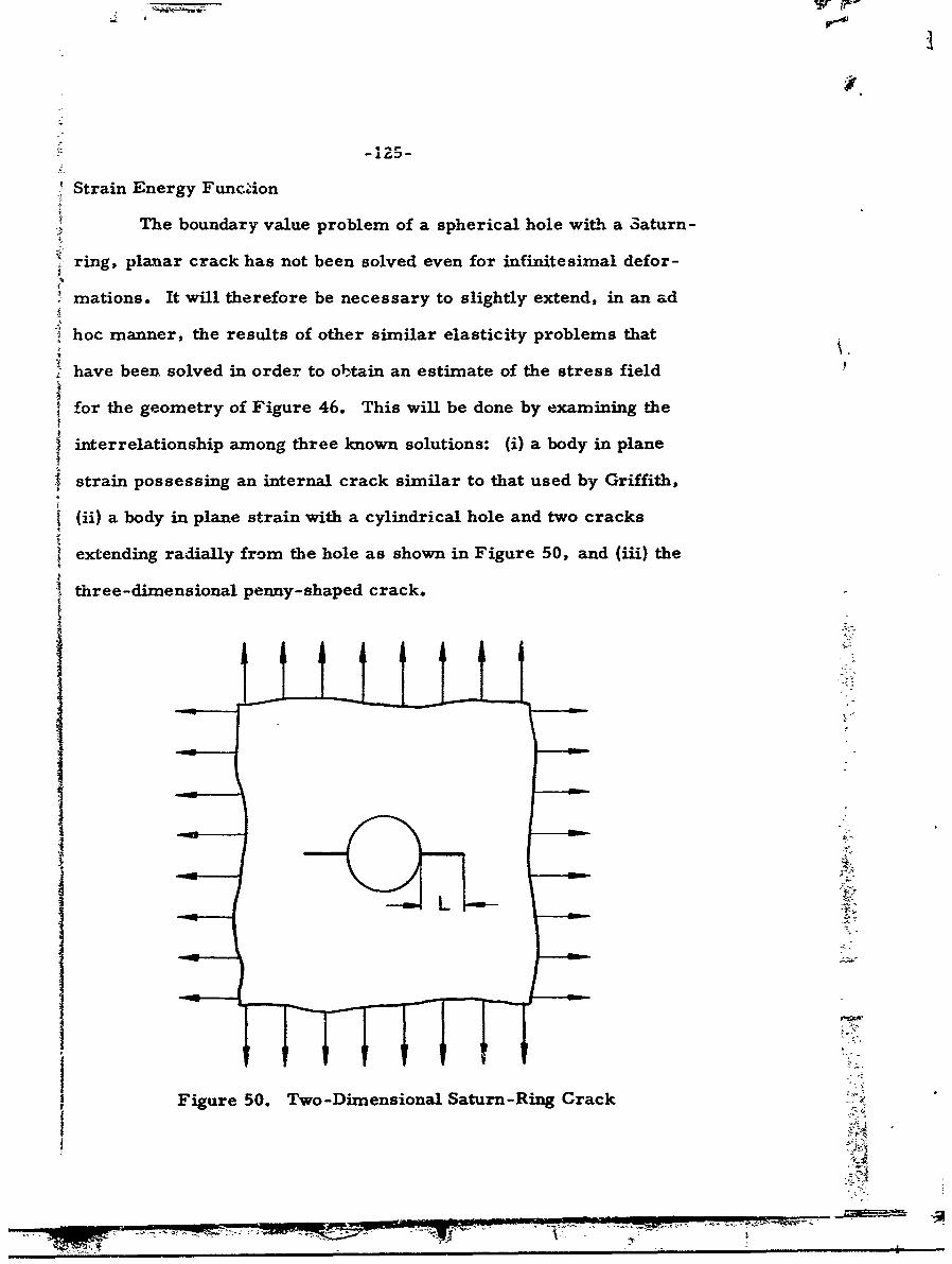
':• -' r2S
Strain Energy Function
The boundary value problem of a spherical hole with a 3aturn-
ring, planar crack has not been solved even for infinitesimal defor-
mations. It will therefore be necessary to slightly extend, in an ad
hoc manner, the results of other similar elasticity problems that
"• have been solved in order to obltain an estimate of the stress field
for the geometry of Figure 46. This will be done by examining the
J interrelationship among three known solutions: (i) a body in plane
Sstrain possessing an internal crack similar to that used by Griffith,
(ii) a body in plane strain with a cylindrical hole and two cracks
extending radially from the hole as shown in Figure 50, and (iii) the
i three-dimensional penny-shaped crack.
i;i
, ~Figure 50. Two-Dimensional Saturn-Ring Crack-"
717I z7F

-126-
In both instances the two-dimensional sheets are taken to be loaded
in equal biaxial tension or what may be roughly referred to as a two-
dimensional hydrostatic tension. Griffith, (66) using the Inglis (80)
solution for the line crack in a two-dimensional sheet, integrated
the stresses and strains for a fixed force loading condition and gave
as the strain energy of the body in plane strain the following:
2 22"(1-v1 p c 0U = U 0 + E (
Let us compare the form of this expression with one obtained from
an approximate solution found by Bowie (81) for the two-dimensional
Saturn-ring
r( 1 -v 2)p 2 L 2 k(L)U = U0 + E(5.2)
L is the half crack length as specified in Figure 54, and k(L) can
be given an analytic representation in three separate regions of the
variable crack length L, by fitting Bowie's tabular data as is shown
in Figure 51.
small L k(L) = 2
intermediate L k(L) = 1 1I +I)2
L 2 2 L1 ~t
"large L k(L) = 1
From this k(L) can be sketched over the entire range of L, and will
appear as in Figure 52.
-77-WU
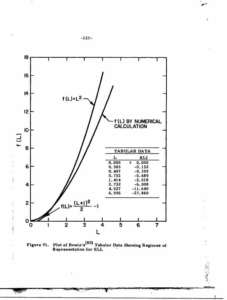
-127-
18 f,
16 -
14f (L)=L 2
12-
f (L) BY NUMERICAL10- CALCULATION
_J
8- TABULAR DATA
L f(L)
0.000 a 0.0006 0.303 -0.152
0.497 -0.3590.732 -0.6891.414 -2.018
4 2. 732 -6. 0084.027 -11.6406.596 -27. 860
2 - -f (L)=2
00I 2 I I I0o0 1 2 3 4 5 6 7
L
Figure 51. Plot of Bowie's18 0 ) Tabular Data Showing Regimes ofRepresentation for f(L).
~I

-128-
L2
V
k(~L)2 --. "- -- ,--
i7.5L
"Figure 52. Crack Length Factor
The inflection point, d 2k/dL = 0, occurs at L 7.5. From this it
is readily seen that there is not a large variation even when the entire
range of L is considered. For the investigation of fracture initiation,
the range for small L is the one desired, and therefore k(L) = 2 will
be selected.
Having made the extension from the two-dimensional line
crack to the two-dimensional Saturn-ring crack, we are now in a
position to make a similar extension from a three-dimensional planar
crack to a three-dimensional Saturn-ring crack. The planar crack,
or so-called penny-shaped crack, shows almost no change from the
line crack except in the dimensionality
2222 3
ir(l-V2 ) p co + (1-v2 2 c3
U=U+ U0 - 00 E 03 E
line crack planar crack
Using the previous example as a guide, it is conjectured that the
strain energy of the three-dimensional Saturn-ring crack could be
approximated as
Men" -;
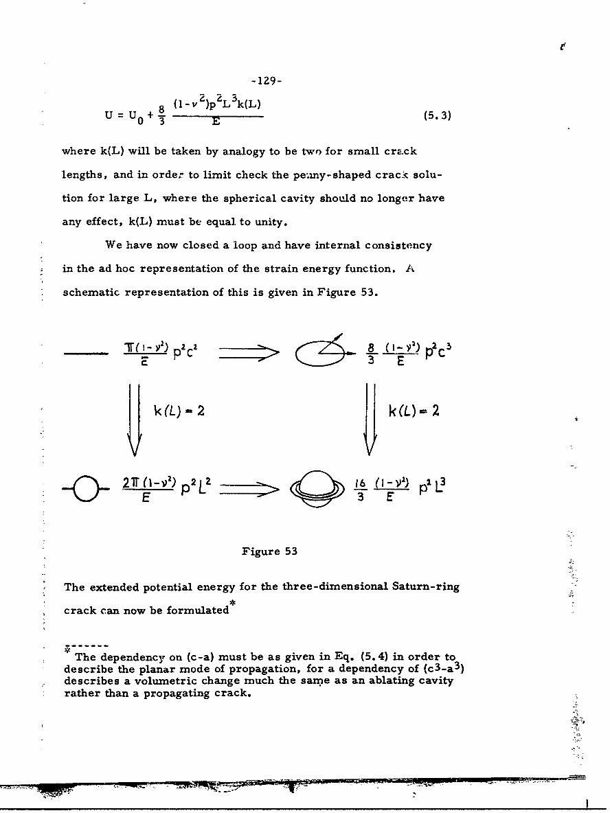
-129-
8 ( - v')p'L'k(L)u =u0 + 8 ( 5.3)
where k(L) will be taken by analogy to be two for small cra.ck
lengths, and in order to limit check the pe-my-shaped crack solu-
tion for large L, where the spherical cavity should no longer have
any effect, k(L) must be equal to unity.
We have now closed a loop and have internal consistency
in the ad hoc representation of the strain energy function, A
schematic representation of this is given in Figure 53.
PC PC~KJI~
k(L) 2 kL) 2
O E 3 E PL
Figure 53
The extended potential energy for the three-dimensional Saturn-ring
crack can now be formulated
The dependency on (c-a) must be as given in Eq. (5.4) in order todescribe the planar mode of propagation, for a dependency of (c3-a 3 )describes a volumetric change much the sanme as an ablating cavityrather than a propagating crack.
Mr.- *
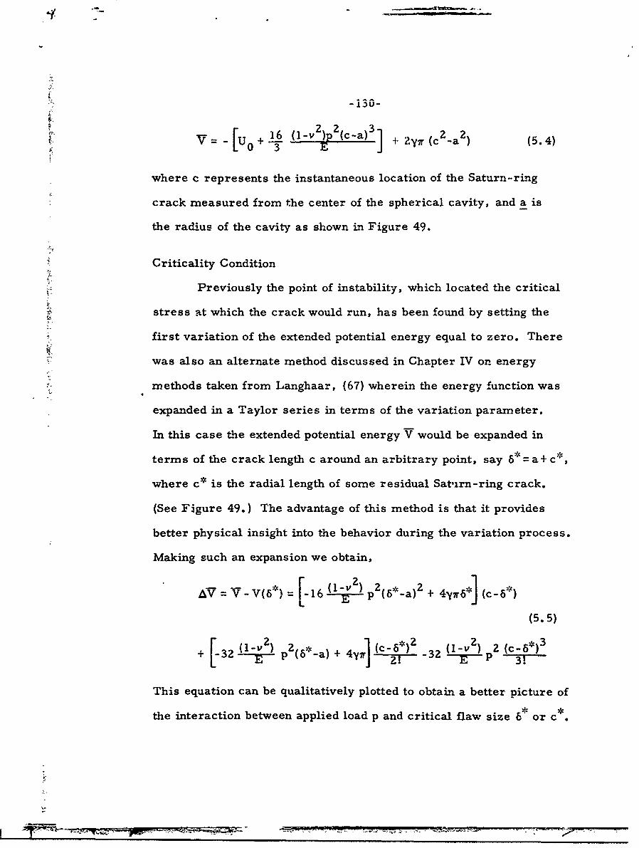
-130-
16(- )up (c-a)3], 0 31 + Zy• (c 2 -a 2 ) (5.4)
where c represents the instantaneous location of the Saturn-ring
crack measured from the center of the spherical cavity, and a is
the radius of the cavity as shown in Figure 49.
Criticality Condition
Previously the point of instability, which located the critical
stress at which the crack would run, has been found by setting the
first variation of the extended potential energy equal to zero. There
was also an alternate method discussed in Chapter IV on energy
methods taken from Langhaar, (67) wherein the energy function was
expanded in a Taylor series in terms of the variation parameter.
In this case the extended potential energy V would be expanded in
terms of the crack length c around an arbitrary point, say 6*= a+ c*,
where c* is the radial length of some residual Satirn-ring crack.
(See Figure 49.) The advantage of this method is that it provides
better physical insight into the behavior during the variation process.
Making such an expansion we obtain,
&v- V(*)= [-16 (1 -) pZ(6*-a)Z + 4y7T6 (c-6
(5.5)
S-32 pZ(6*-a) + 4y 21 -32 P 3!
This equation can be qualitatively plotted to obtain a better picture of
the interaction between applied load p and critical flaw size 6 or c
- - -~or C,--

-131-
A p increasinr
IC
Figure 54. Adjusted Potential Energy vs. Crack Lengthi
It was previously shown that AV was actually related to the slope;
4 i.e., the first variation around this loaded ,;tate corresponded to a
} second variation around the unloaded state, and the point of interest
.! is where the slope changes signs, or where the function AV crosses
the horizontal axis. The actual point at which it crosses the axis
is a function of the parameter P, and the point of crossing is 6 *
If we investigate the function for values of crack length very near
6 the first term is dominant, and the point at which the derivative
changes sign can be closely approximated by setting the first term
of equation (5.5) equal to zero.
E -a yr6 (5.6)
or
4(1 -v) c + a "/aEy(r * (5.7)
c
-132-
Physical Interpretation
The physical interpretation of this variation or more specifi-
cally c is not absolutely fixed, but it can be adapted to the physical
processes involved in the fracture of S-1 13. It is clear from Figure
54 that as p increases, the residual Saturn-ring flaw c * must de-
crease; however, in the limit as c approaches zero, or in: other
words, in the limit of fracture of the spherical cavity alone without
a Saturn-ring crack, the critical stress approaches infinity, as seen
from (5.7) in the same manner as the original Griffith result. This
is not actually true, for if one examines the atomic level, there is
always a Saturn-ring flaw of the order of atomic dimensions, but
this goes beyond the applicability of the continuum theory, and so
it is appropriate to seek another interpretation of c
By visual inspection of virgin S-1 13 under microscopic
powers of 600X to 8OOX, the continuum around the flaw appeared
to be intact, and there was certainly no Saturn-ring flaw initially.
However, it is believed from observing the experiments, that the
actual fracture occurs in this Saturn-ring mode, from which it may
be concluded that the material, after a fashion, grows its own flaw.
To elaborate on this point, imagine that as an observer we are
allowed to go inside the spherical cavity and watch the fracture
as it initiates at that surface. As the load is applied at infinity,
we would notice bonds beginning to break at various points on the
surface where the stress is the highest; however after the first bond
has broken, the material would still remain intact and fiacture of
the specimen would not occur. This bond breakage would not be

-133-
discerned by an outside observer, for he would have no way of de-
tecting it so we arrive at the tedious point of defining where fracture
actually starts. If it is not defined to occur at the rupture of the
first bond, is it at the point of the seventh bond, or at the one-
hundredth bond, or where is it?
Knauss (82) has devoted some attention to this problem as
he has studied the propagation of cracks in sheet geometries at
various velocities, and has arrived at this same conclusion - that
a body will grow its own flaw. He has shown that for an H-C rubber,
which is similar in many respects to S-113, the fracture surface
characteristics change dramatically as the velocity changes, and
that there are three distinct regions as-he classified them. The
first or slowest velocity regime is characterized by a very rough,
cobbled surface where the fracture appears as if strands resembling
rubber bands were pulled apart individually. This regime is for
very low velocity crack propagation. The second regime, which
he terms the transition region, is more smooth in appearance and
much less cobbled. In the high velocity region, the fracture surface
appears glassy and mirror-like. A plot of the crack propagation
speed versus the gross stress applied to a sheet geometry is ex-
cerpted from this work (82) and shown in Figure 55. In that figure
is contained the evidence of a very rapid change in velocity versus
applied stress for certain ranges; in fact, in the slowly propagating
regime, evidenced by a very rough surface, the velocity to a good
approximatiun could be taken to be zero. It is this mechanism that
is employed here to define c and to interpret the manner in which
F r-- -~-
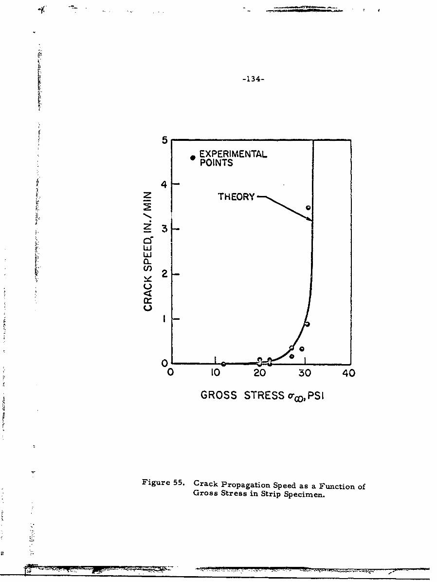
-134-
P
I
• 5
- EXPERIMENTALPOINTS
4SZ THEORY
13
U
"'2_
I-
0
0 10 20 30 40
GROSS STRESS o-,PSI
Figure 55. Crack Propagation Speed as a Function ofGross Stress in Strip Specimen.
-4747
IL

a body grows its own flaw.
Let us now return to the spherical cavity problem. As the
stress increases to some limit point, a few bonds are broken and
eventually as the stress is increased, enough broken bonds will occur
in a localized region to create a microscopic crack, and this micro-
scopic crack is propagating at almost zero velocity, as shown in
Figure 55. But given enough time, the specimen will eventually
rupture. Strictly speaking, the crack is unstable and the critical
stress has been reached, but it goes undetected and may continue
moving slowly for a long indefinite period. In this application the
interest is in elastic fracture, and the rate effects can be ignored
by assuming that the velocity of propagation is zero and that the
body, as a result of the applied load, has created a microscopic flaw,
which is perfectly stable and which will not run. As the load is in-
creased further, the flaw will be made larger, but it will remain
• stable. Referring back to Figure 54, it is seen that the allowable
flaw size is becoming smaller as the load is increased; thus the
two variable parameters are approaching each other. As the applied
4 hydrostatic pressure is increased, the critical flaw size that tht. body
i can withstand is decreased, but the actual flaw size is increasing at
• virtually zero velocity. Finally, the point will be reached where
the flaw grown by the material becomes critical for the applied
load and at that instant the flaw will become unstabie, producing
fracture of the entire specimen. Interpreted in light of the velocity
I results of Knauss, at that point the velocity will change from zero
4 to the high velocity propagation level. It is at this point that

"FN -136-
fracture is defined by the observer on the outside of the specimen,
for, by virtue of the energy releasbd, a manifestation appears at the
loading device of the testing machine, or by visual observation,
the crack has become large enough that it can be observed as it.
propagates. It is this interpretation that is given to c*. It is tke
size of a critical flaw grown during the loading process, emanating
[ from the surface of the residual spherical cavity, and acting as a
stress riser to produce fracture nucleation.
U Limit Cases. It is convenient to cast equation (5.7) in terms
of non-dimensional variables. Let us define • = c*/a, then equation
( (5.7) becomes
2 pZ + (5.8)p a 2
In the limit of g becoming large, or where the parameter c* is large
compared to the bubble radius a,
p2 1~ Z -. I(5.9)
c
which is a constant independent of the initial flaw size a. (It should
be noted that it is not independent of the existence of a cavity - only
its size.) Thus as the flaws become small compared to the fracture
parameter c*, they have no influence on the fracture and cause no
damage to the material. They act only as nucleation points.
On the other hand, the limit of t becoming small, where the
cavity is the dominant factor
p2 a (5.10)c
-- ~ ~ ~ ~ 7 7"--- - --

-137-
and the large cavity causes an increase in the fracture strength over
smaller cavities -- not over the perfect material. It behaves in
much the same way that a large fillet radius does, causing a reduc-
tion in the stress concentration in a body and a consequ-,nt increase
in strength. In the intermediate values, there is an interplay of the
various parameters that can be qualitatively plotted as shown in
Figure 56.
p2
a increosirl9
0Figure 56. Critical Pressure vs. Flaw Size
This rather unusual result arising from the diameter term of equa-
tion (5.7) which indicates that the larger bubble will sustain more
load before fracture was in keeping with the observed behavior. The
theory predicts that for a fixed c*, fracture would initiate at the
smallest bubble in the matrix; however, in the poker-chip test there
would be a trade-off between the size of the flaw and the location
in the field due to the stress decreasing radially from the center.
Consequently the actual pinpoint location would involve an interplay
between the field stress and the size of the flaw. As a result, we
have employed the average flaw size to compute the theoretical
-138-
strength of the material, since this size flaw would have the highest
probability of occurring at the point of maximum stress. However,
statistical variations in cavity size and location would be partially
responsible for strength variations. It would be predicted from
equation (5. 10) that if the larger artificially inserted bubble had
been alone in the field, an appropriately larger fracture stress
would have resulted; however the presence of the smaller cavities
caused the fracture to nucleate from them and the fracture levels
to remain unchanged, even with the presence of the large flaw.
Numerical Correlation. In order to demonstrate this theory
further, a theoretical computation of strength will be made based
on measurements of a flaw size a and 65, takcn from a typical
specimen. From Figure 34, 6* is measured as 3.7 x 10⁻⁴ in.
Assuming that the iracture resulted from a typical cavity of radius
a= Z x 10-4, c* is computed to be 1.7 x 10⁻⁴ in. With these
figures, all that is required to compute the critical stress is the
surface energy density. This was measured in a separate exper-
iment on a different configuration entirely. A two-dimensional
sheet containing a crack was extended in plane stress. The con-
figuration was adjusted to approximate a sheet of infinite extent
with a semi-infinite crack, as shown in Figure 57.
Figure/ 57./ Shet C/.g r
Figure 57. Sheet Configuration Used for Measuring Surface Energy
,• ~l ,•__.••, • .•.. .... .__.• __ • , ,..'-•.•=--•.-•.--= .. --w•-:. -- , . ........ .. ... ,
-139-
By plotting the propagation velocity of the crack vs. the applied
strain at the boundary, an approximate measure of the strain at
which the crack propagates at virtually zero velocity can be ob-
tained. At this point it is assumed that kinetic energy and dis-
sipation are minimal; therefore the strain energy is directly
converted to surface energy as the crack moves ahead. Equat-
ing the two, y comes out to be 0.05 in lb/in 2. The actual value
for y is taken to be a material property independent of geometry
and thus applicable in this analysis for HT.
Putting these values into equation (5.7) and using E =1
500 psi and v =
Pcr = 580 psi
This is very near the recorded fracture value of 625 psi for the
specimen from which these mneasurements were taken. Figure
29 is the apparent stress-strain curve for this specimen, which
exhibits an apparent fracture strain of . 026 in/in. From Figure
8, az/E = 48, where z cr and the measured value of thez z c
local hydrostatic pressure in 625 psi. Such good agreement may
be a bit fortuitous, but it lends support to the validity of the
theory and calculations.
Thus the Saturn-ring concept, with the accompanying
calculations, is able to predict experimental results as well
as provide a plausible explanation for the observations made
with the large, artificial flaws. The results forthcoming from
the analysis are of considerable interest when discussing the
1 - 0- pop wa i4
-140-
difference between cavities and cracks. The energy formulations
show that they enter the problem in a fundamentally different way,
as seen by comparing equation (5.7) to Sneddon's result, for in-
stance. It is true that for a crack the larger its size, the less its
endurable load; however cavities do not act this way. The compara-
tive results between the two continues to behave as intuitively ex-
pected; i.e., a body possessing a cavity, for a hole, of the same
dimension as a crack would be expected to withstand more stress,
or would bear more load than the cracked body and this is exactly
what the energy expressions predict. The exact manner in which
the cavity radius enters is extremely interesting. It shows that in
some regimes the cavity is not important at all except in acting as
a nucleation point and lends a new concept about the effect or resid-
ual cavities in rubbery materials, or other materials for that mat-
ter, and their effect upon the malfunctioning of that body. Heretofore
it has been the intuitive feeling that has motivated quality control
techniques, which accepts a structure that has flaws under a speci-
fied size and discards as inacceptable bodies containing flaws that
would exceed this randomly selected size. This result will have
significant meaning for people engaged in such work, for it demon-
strates that another piece of information, c*, must be known before
a decision can be made. It must be emphasized in conclusion that
this application is for hydrostatic tension only and may be much
different in another geometry; in fact, it will be demonstrated that
this actually is the case in the next section.
--.... *-, i -NI - m M- - .I-

-141-
RELATED GEOMETRIES
Although the purpose of this study was to investigate hydro-
static fracture, the unusual nature of the cL/ity size dependency
makes it intriguing to know what other geometries wiln yield. A
brief look at the two-dimensional analogy, consisting of a cylin-
drical, hole in equal biaxial tension, provides additional under-
standing of the role of cavities as opposed to cracks. Returning
again to the Bowie (81) solution, the expression for the extended
potential energy becomes
2 2V =U 0 - E (c-a) + 4y(c-a) (5.11)
where a = radius of the original cylindrical hole
c = length of the crack measured from the periphery of
the hole
The critical condition obtained by expanding V in a Taylors Series
about a given crack size c is
Pcr (512)
when c* ýs again taken as the crack dimension "grown" in the ma-
terial by the loading at zero velocity before the fracture process
becomes unstable.
This is an interesting turn of events, because the initial
hole size, a, does not appear explicitly. It does influence the ex-
pression for strain energy (5. 10), since this is dependent upon
geometry; however the influence is the same regardless of the
size of the hole. This statement should be tempered with the fact
,4

~- 142-
that the hole must be small compared to specimen dimension. Fur-
thermore the theory assumes that fracture occurs simultaneously
over the entire thickness of the specimen. Although this assumption
is standard for the reason that the thickness effect is a separate
study in and of itself, (83) it is exceptionally crucial in this instance.
It directly affects the form of the surface energy expression, which
is the term that gives rise to the appearance of the initial cavity
size in the criticality condition. Within these limitations the frac-
ture stress should be independent of initial hole, or cavity, size.
Experimental Results
A few preliminary tests have been run to evaluate this pre-
diction. Only a small number of runs were made for equal, biaxial
tension, but a significant number of specimens were tested in uni-
axial tension. For the biaxial tests, specimens were prepared by
casting large, circular sheets 13 inches in diameter and 0. 10 inches
thick in the standard way. After curing, the central portion of the
sheet was frozen with liquid nitrogen, which made it possible to
drill holes with smooth surfaces free of stress concentrations. The
equal biaxial stress field was produced by inflating this membrane
.ith the central cylindrical hole by a pressure apparatus similar to
that of Figure 4. Loading the sheets to failure for a series of holes
of 1/16, 1/8 and 1/4 inches in diameter, fracture stresses of 109
psi, 123 psi, and 116 psi respectively were recorded. For all
intents and purposes this can be considered constant. These exper-
iments are by no means conclusive, but they do display the trend
-143-
predicted by equation (5.12), and one statement that can be made is
that the dependency of hole size does not appear to be inverse square
root as is the case for cracks.
Of course, the same geometry loaded by a one-dimensional
stress field does not possess fundamentally different energy expres-
sions from the two-dimensional case; consequently, the critical
pressure possesses the same form except for the magnitude of
constants. A series of tests was run for uniaxial specimens con-
taining cylindrical holes, ranging in size from 0.03 to 0. 525 in.,
or over approximately a one decade spread. The specimens were
3"t x 4" x 0.10"1 giving a specimen width to cavity ratio of the
orders of 10 to 100. Results of the test are plotted in Figure 58,
where a remarkable demonstration of the predicted result of equa-
tion (5. 12) is manifested. The fracture level is constant except
for a small transition region where the cavity sees a change from
the plane stress environment to plane strain. In other words, when
the hole size is large compared to the thickness it sees a plane
stress field, but as the hole size is reduced, it finally becomes
approximately the same magnitude as the specimen thickness.
From this point on, the hole sees a plane strain field and the energy
enters the process, as well as the fracture equation (5.10). in a
slightly different way. The strain energy is altered by a factor
of 1/l-V and the critical stress is increased by the square root of
this quantity. For purposes of a nearly incompressible material
such as S-113, the factor becomes 1. 15. This is almost exactly
the increase that is observed experimentally in Figure 58 as the

Ilk,
I AA
I F C
w4)
00
wZI.L 0
<~WpCl4)
0
t..
0 (l) c
Zc/)
211Iz
Zr')
00 0 "%4
000
-4
-145-
fracture level changes from 31.5 to 36.0 on the average.
This brief side excursion from hydrostatic fracture suggests
additional corroboration of the concept of a flaw "grown" by the
loading, which concept appears to predict rather accurately the
experimental results. Ii further quggests some alterations in one's
intuition with regards to the effects of the dimensionality of the
stress field and the influence of cavity size on fracture level. The
general trends noted here can be nicely fit into the stress-axis
theorem on fracture, alluded to previously, to provide guidelines
for engineering analysis -Ad design.
Character of c
One additional item of interest is the correlation of the con-
cept of an actual numerical value of c* in the various stress fields.
At this point it is not possible to deduce a dependency of c* on
geometry or material properties; i.e., whether it is predominantly
determined by the geometry of a stress field or whether there is a
fundamental mechanism tied up with the chain structure that dictates
2c the magnitude of the flaw that must be grown before it becomes un-
stable and propagates at high velocity. Additional experimental
work will have to be conceived and carried out to define the exact
properties of c*. Along this same line is the product of the mater-
ial properties Ey which always arise in any fracture analysis,
indicating that a wide range of materials possessing a diversity of
mechanical properties could still fracture at the same point if the
EY product remained the same. In other words a more glassy
-146-
polymer possessing a high modulus may at the same time have a
low surface energy density and still fracture at the same point as
a rubbery polymer with a low modulus and a high surface energy
density, providing c* is the same. This reasoning attributes addi-
tional importance to the fundamestal nature of c* as describirng
the difference in chariacter of the fracture between two materials
of this type--if there is a difference.
SUMMARY
In summary it is felt that the results of the poker-chip ex-
periments on both the standard material and the material with the
artificial flaws have-amplydemonstrated that the mechanism of poly-
mer fracture through a Saturn-ring crack, whereby the material
generates its own flaw, is a reasonable one. Furthermore the pre-
liminary results of the one and two-dimensional tests seem to attest
the conclusion reached in the three-dimensional analysis that the
hole, or cavity, size affects fracture properties in a manner com-
pletely different than a crack. Having touched all of the bases, so
to speak, it appears that a consistent story has been generated
that has been verified experimentally, from which extensions can
now be made to the more general case where holes and cavities
are analyzed in the viscoelastic range.

CHAPTER VI
CONCLUSION
At this point it is appropriate to assemble in brief form the
main contributions of this study in an effort to integrate the several
parts into a whole, and to better delineate what progress has been
made. A lot of groundwork has been laid in the form of experimental
test development, specimen stress analysis, etc. that wil continue
to be useful in further triaxial fracture studies. Results of exper-
imental tests employing these tools have provided quantitative
definition of ultimate strengths in hydrostatic tension, which pro-
vides the limit point for the topological fracture surface in principal
stress space.
The discovery, measurement and distribution analysis of
spherical cavities in the material has given better insight to guide
the theoretical treatment of flaws. Furthermore it has identified
a type of material that can be used for extensive investigation of
cavity flaw behavior. It may also lead to the identification of other
materials of a similar classification, which possess inherent flaws
due to manufacturing and processing. These steps forward all have
applications beyond the scope of this particular study and may be
readily employed in extensions of this work.
The application of energy methods of fracture analysis to
spherical cavities has led to predictions of ultimate strengths,
both for finite and infinitesimal deformations, which compare
favorably with experiment in some regimes; however many of the
same problems that plagued Griffith in his initial work with energy
MMM
-148-
analysis still plague u.s today. By this it is meant that from the
standpoint of fundamental physical processes involved, a great deal
still remains to be learned. For instance Griffith (66) performed
experiments on glass that he used as evidence of his theoretical
predictions. In many respects they did not duplicate the conditions
imposed in the mathematical treatment, and this continues to be,
and promises to remain, a challenge to the experimentor. To
accurately duplicate the ideal boundary conditions is a tedious and
difficult task. In addition, he required the surface energy of the
glass as a parameter in the expression for critical stress. Since
he could not measure this quantity in the solid state, he used the
liquid value as an approximation. In the intervening forty years
since Griffith published his work, the colloidal chemists have been
studying surfaces, or more accurately, in.erfaces, and have
learned a great deal about them. Most of this knowledge, however,
has pointed to the fact that it is a much more complicated phenome-
non than had been originally appreciated, and the concept of surface
energy in solids is still quite nebulous. So that just exactly what
surface energy is in solids and the mechanisms involved in creating
a surface duxing fracture still remain as missing pieces in the
puzzle. Suci- '.-y pieces are worthy of study and constitute a logical
avenue of further research.
Another finding of this study relates to the difference in
eLffect on the strength of a body c o n t a i n i n g cracks and cavities.
Once again the confidence level in the results is limited by the lack
of understanding of the basi.c processes. The energy approach used
'I
-149-
seems to be sound and well motivated mathematically; however
the separate terms in the analytical expressions strongly depend
upon the physical mechanisms and how accu.ate•y they can be
described mathematically. In cracks this is a little better defined
than in cavities, since propagation details can be formulated more
readily on an intuitive basis. The manner in which a spherical
cavity opens up into a crack is not at all obvious. As a result of
this study, which has concentrated on discovering some of the
fundamental mechanisms, additional insight into the behavior of
cavities as fracture nucleation points has been obtained. How-
ever most of this information has been gleaned from evidence left
on the fracture surface; consequently the hypothesis of the Saturn-
ring propagation mode is predominantly inference and, although
it seems to explain all of the phenomena, the evidence is still not
conclusive. In other words, from almost any standpoint there is
a need for extensive fundamental studies on elastic fracture pro-
cesses. These items will also constitute a valuable contribution
when dissipative effects of viscoelastic materials are included,
or when dealing with the more complicated filled material.
-
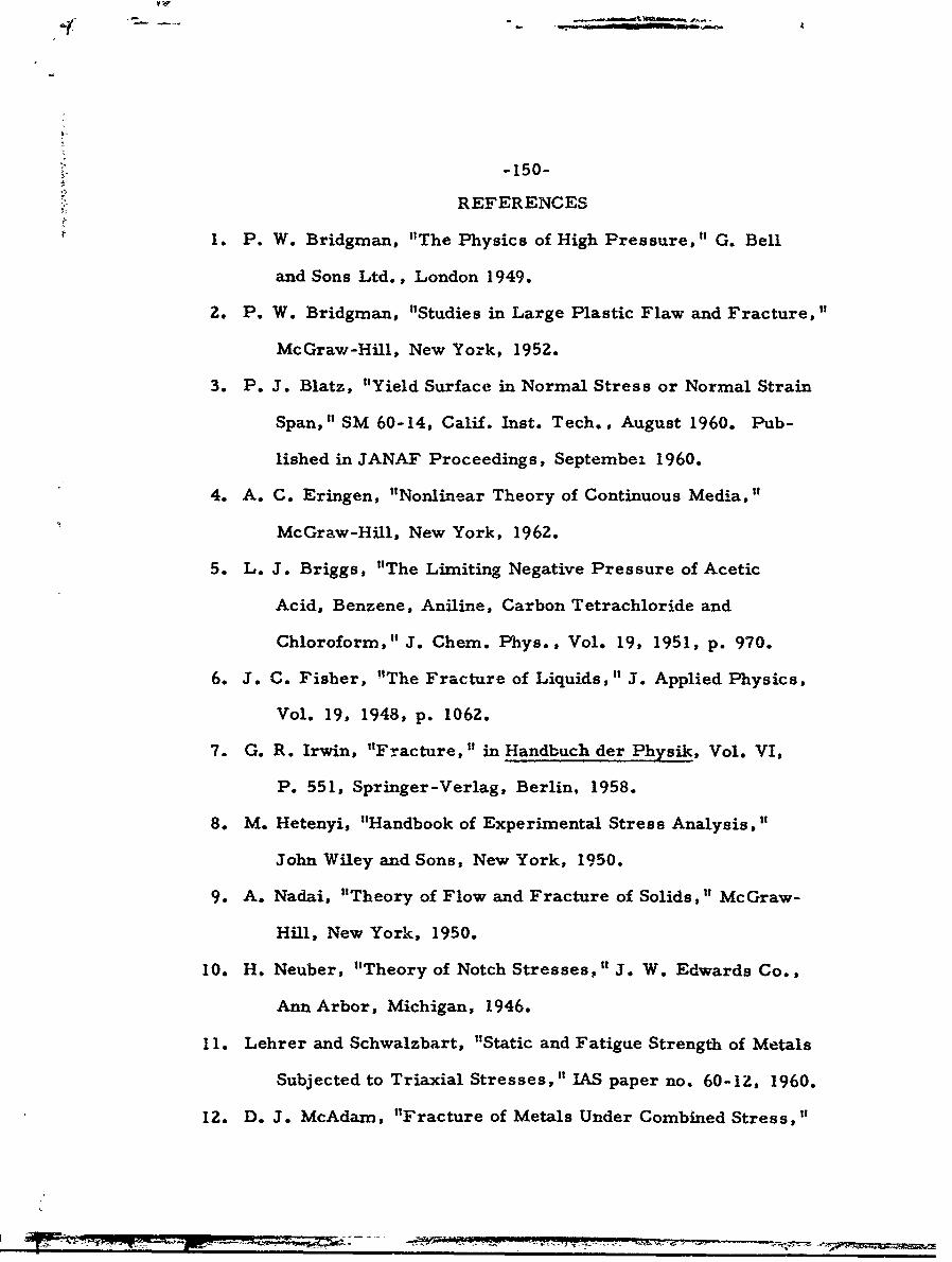
-150-
REFERENCES
1. P. W. Bridgman, "The Physics of High Pressure," G. Bell
and Sons Ltd., London 1949.
2. P. W. Bridgman, "Studies in Large Plastic Flaw and Fracture, "
McGraw-Hill, New York, 1952.
3. P. J. Blatz, "Yield Surface in Normal Stress or Normal Strain
Span," SM 60-14, Calif. Inst. Tech., August 1960. Pub-
lished in JANAF Proceedings, Septembei 1960.
4. A. C. Eringen, "Nonlinear Theory of Continuous Media,"
McGraw-Hill, New York, 1962.
5. L. J. Briggs, "The Limiting Negative Pressure of Acetic
Acid, Benzene, Aniline, Carbon Tetrachloride and
Chloroform," J. Chem. Phys., Vol. 19, 1951, p. 970.
6. J. C. Fisher, "The Fracture of Liquids, " J. Applied Physics,
Vol. 19, 1948, p. 1062.
7. G. R. Irwin, "Fracture," in Handbuch der Physik, Vol. VI,
P. 551, Springer-Verlag, Berlin, 1958.
8. M. Hetenyi, "Handbook of Experimental Stress Analysis,"
John Wiley and Sons, New York, 1950.
9. A. Nadai, "Theory of Flow and Fracture of Solids," McGraw-
Hill, New York, 1950.
10. H. Neuber, "Theory of Notch Stresses," J. W. Edwards Co.,
Ann Arbor, Michigan, 1946.
11. Lehrer and Schwalzbart, "Static and Fatigue Strength of Metals
Subjected to Triaxial Stresses," 1AS paper no. 60-12, 1960.
12. D. J. McAdam, "Fracture of Metals Under Combined Stress,"

I
-151-
ASM Vol. 37, 1946, p. 538.
13. T. Alfrey, "Mechanical Behavior of High Polymers," Inter-
science Publishers, New York, 1948.
14. F. Bueche, "Physical Properties of Polymers, " Interscience
Publishers, New York, 1960,
15. P. J. Flory, "Principles of Polymer Chemistry, " Cornell
Univ. Press, Ithaca, New York, 1953.
16. M. L. Williams, "Structural Analysis of Viscoelastic Materials,
AJAA, Vol. 2, No. 5, May 1964, pp. 785-809.
17. A. M. Bueche and J. P. Berry, "The Mechanism of Polymer
Failure," in Conference on Fracture. held at Swampscott,
Mass., 1959.
18. M. L. Williams, "Fracture of Viscoelastic Materials, " in
Fracture of Solids, Interscience Publishers, New York, 1963.
19. M. L. Williams, P. J. Blatz, R. A. Schapery, "Fundamental
Studies Relating to Systems Analysis of Solid Propellants,
SM 61-5, Calif. Inst. of Tech., February 1961.
20. R. F. Landel and R. F. Fedors, "Rupture of Amorphous,
Unfilled Polyrners," in Fracture Processes in Polymeric
Solids, Interscience Publishers, New York, 1964.
21. W. G. Knauss and E. Betz, "Some Characteristic Functions
Pertinent to Failure of Viscoelastic Materials," SM 65-16,
Calif. Inst. of Tech. Published in Bulletin of 4th Annual
Meeting of ICRPG Working Group on Mech. Behavior,
Nov. 1965.

• -152-
* W. L. Ko, Application of Finite Elastic Theory to the Behavior
of Rubber-like Materials," SM 63-13, Calif. Inst. of Tech.,
Ph.D. Thesis, 1963.
23. A, N. Gent and P. B. Lindley, "The Compression of Bonded
Rubber Blocks," Journal of British Rubber Producers
Research Association, Vol. 173, p. 111, 1959.
24. A. N. Gent and P. B. Lindley, "Internal Rupture of Bonded
Rubber Cylinders in Tension," Proc. of Royal Society,
Vol. 249A, 1959, p. 195.
25. F. L. Yerzley, "Industrial Engineering Chemistry," Vol. 31,
1939, p. 950.
26. R. Houwink, "The Strength and Modulus of Elasticity of Some
Amorphous Materials Related to their Internal Structure,"
Trans. of Faraday Soc., Vol. 32, 19.-6, p. 12Z.
27. P. J. Flory, "Effects of Molecular Structure on Physical
Properties cf Butyl Rubber," Industrial and Engineering
Chemistry, Vol. 38, No. 4, 1946, p. 417.
28. P. J. Blatz, N. George, S. Kawabata, "Physico-Mechanical
Behavior of Rubberlike Materials," MATSCIT-PS 65-a,
Calif. Inst. of Tech., April 1965.
29. W. G. Knauss, "Rupture Phenomena in Viscoelastic Materials",
SM 63-10, Calif. Inst. of Tech., Ph.D. Thesis, 1963.
30. G. H. Lindsey, "Energy Criteria for Elastic Fracture,
SM 65-20, Calif. Inst. of Tech., August 1965.
31. J. D. Ferry, "Viscoelastic Properties of Polymers," John
Wiley and Sons, New York, 1961.
4-0 - _-W,--

-153-
32. L. R. G. Treloar, "The Physics of Rubber Elasticity," Oxford
Press, London, 1958.
33. R. A. Schapery, "An Engineering Theory of Nonlinear Visco-
elasticity with Applications," A and ES 65-5 Purdue Univ.,
June 1965.
34. G. Pickett,"Application of the Fourier Method to the Solution
of Certain Boundary Problems in the Theory of Elasticity,"
Journal of Applied Mechanics, Vol. 11, Sept. 1944, p. A-176.
35. A. R. Zak and M. L. Williams,"Crack Point Stress Singulari-
ties at a Bimaterial Interface,' SM 62-1, Calif. Inst. of Tech-
nology, 1962.
36. E. C. Francis and D. Cantey, "Structural Integrity of Propel-
lant Grains," Lockheed Propulsion Company, Report No.
556-F, January 1963.
37. M. L. Williams and R. A. Schapery, "Studies of Viscoelastic
Media," Aeronautical Research Laboratories, Wright-
Patterson Air Force Base, Ohio, ARL 62-366, June 1962.
38. A. N. Gent, Proceedings of the Rubber Engineers Confer-
ence, 1956, p. 25.
39. A. M. Messner, "Stress Distribution in Poker Chip Tensile
Specimen," Second Meeting Bulletin of ICRPG Working
Group on Mechanical Behavior, CPIA Pub. No. 27, Oct.
1963, p. 109.
40. J. J. Brisbane, "Stresses, Strains and Displacements in the
Pokerchip Test Specimen," Report No. P-63-13, Quarterly
Progress Report on Engineering Research, Rohm and Haas
MEWW"
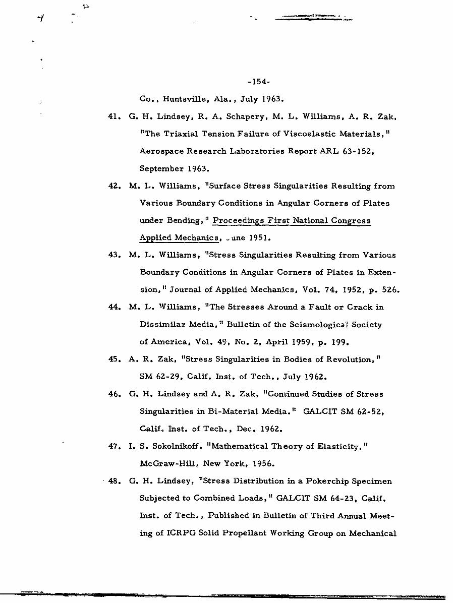
-154-
Co., Huntsville, Ala., July 1963.
41. G. H. Lindsey, R. A. Schapery, M. L. Williams, A. R. Zak,
"The Triaxial Tension Failure of Viscoelastic Materials,"
Aerospace Research Laboratories Report ARL 63-152,
September 1963.
42. M. L. Williams, "Surface Stress Singularities Resulting from
Various Boundary Conditions in Angular Corners of Plates
under Bending," Proceedings First National Congress
Applied Mechanics, - une 1951.
43. M. L. Williams, "Stress Singularities Resulting from Various
Boundary Conditions in Angular Corners of Plates in Exten-
sion, " Journal of Applied Mechanics, Vol. 74, 1952, p. 526.
44. M. L. Williams, "The Stresses Around a Fault or Crack in
Dissimilar Media, :' Bulletin of the Seismological Society
of America, Vol. 49, No. 2, April 1959, p. 199.
45. A. R. Zak, "Stress Singularities in Bodies of Revolution,"
SM 62-29, Calif. Inst. of Tech., July 1962.
46. G. H. Lindsey and A. R. Zak, "Continued Studies of Stress
Singularities in Bi-Material Media." GALCIT SM 62-52,
Calif. Inst. of Tech., Dec. 1962.
47. I. S. Sokolnikoff. "Mathematical Theory of Elasticity,"
McGraw-Hill, New York, 1956.
48. G. H. Lindsey, "Stress Distribution in a Pokerchip Specimen
Subjected to Combined Loads," GALCIT SM 64-23, Calif.
Inst. of Tech., Published in Bulletin of Third Annual Meet-
ing of ICRPG Solid Propellant Working Group on Mechanical
-155-
Behavior, Oct. 1964.
49. S. Timoshenko and J. N. Goodier, "Theory of Elasticity,"
McGraw-Hill, New York, 1951.
50. W. G. Knauss, "A Cross-.Linked Polymer Standard Report on
Polymer Selection," MATSCIT Report PS 65-3, Calif. Inst.
of Tech., April 1965.
51. A. R. Zak, "Multiaxial Failure of Viscoelastic Materials,"
Aerospace Research Laboratories ARL 64-144, Sept. 1964.
52. M. L. Williams, R. J. Arenz, "The Mechanical and Optical
Characterization of Solithane 113," Second International
Congress on Experimental Mechanics, Washington, D. C.,
Sept. 1965.
53. W.G. Knauss, "A Cross-Linked Polymer Standard Report on
Polymer Selection," MATSCIT Report PS 65-3, Calif. Inst.
of Tech., April 1965.
54. A.R. Zak, "Uniaxial Characterization of Solithane 113 Visco-
elastic Properties," GALCIT SM 64-37, Calif. Inst. of Tech.,
Aug. 1964.
55. M. L. Williams, R. F. Landel and J. D. Ferry, J. American
Chemical Society, Vol. 77, 1955, p. 3701.
56. R. J. Arenz, C. W. Ferguson, T. Kunio, M. L. Williams,
"The Mechanical and Optical Characterization of Hysol 8705
with Application to Photoviscoelastic Analysis," Tech. Docu-
mentary Report No. WLTDR 64-4, June 1964.
57. T. L. Smith, "Stress-Strain-Time Temperature Relationship
for Polymers," Reprint from Symposium on Stress-Strain-
-156-
Time Temp. Relationships in Materials, Special Technical
Publication No. 325, ASME.
58. S. W. Beckwith and G. H. Lindsey, "Finite Strain Character-
ization of Solithane 113," GALCIT SM 65-15, Calif. Inst. of
Tech., August 1965.
59. D. F. Miner and J. B. Seastone, "Handbook of Engineering
Materials," John Wiley and Sons, New York, 1955.
60. B. C. Harbert, "Triaxial Tensile Failure of Solid Propellants,
Bulletin of Third Annual Meeting of ICRPG Working Group
on Mechanical Behavior, Vol. I, November 1964.
61. M. Levinson and P. J. Blatz, "The Finite Plane Strain Defor-
mation of a Thin Pad." GALCIT SM 64-5, Calif. Inst. of
Tech., March 1964.
62. E. Betz, "Some Mechanical Properties of Solithane 113,"
GALCIT SM 65-12, Calif. Inst. of Tech., July 1965.
63. W. G. Knauss, "The Time Dependent Fracture of Viscoelastic
Materials," GALCIT SM 64-47, Calif. Inst. of Tech. -
Preprint International Conference on Fracture, Sendai,
Japan, Sept. 1965.
64. W. G. Knauss, "On the Mechanical Properties of an H-C
Rubber, Bulletin of Second Mtg. of ICRPG Working Group
on Mechanical Behavior, Oct. 1963, p. 179.
65. E. Orowan, "Fracture and Strength of Solids," In Report on
Progress in Physics, Physical Soc. of London, Vol. 12,
1949, p. 185.
66. A. A. Griffith, "The Phenomena of Rupture and Flow in Solids,
-157-
Phil. Trans. of Royal Society, Series A, Vol. 221, 1921.
67. H. L. Langhaar, "Energy Methods in Applied Mechanics,"
John Wiley and Sons, New York, 1962.
68. L. A. Pars, "On Introduction to the Calculus of Variations,"
John Wiley and Sons, New York, 1962.
69. A. E. H. Love, "The Mathematical Theory of Elasticity,"
Oxford Press, London, 1927.
70. I. N. Sneddon, "The Distribution of Stress in the Neighborhood
of a Crack in an Elastic Solid," Proc. Royal Society, Series
A, Vol. 187, 1946, p. 229.
7 1. R. A. Sack, "Extension of Griffith's Theory of Rupture to
Three Dimensions, " Proc. Physical Soc. of London, Vol.
58, 1946, p. 729.
72. A. A. Griffith, "The Theory of Rupture," Proceedings of the
First International Congress for Applied Mechanit s, 1924.
73. M. L. Williams, "Initiation and Growth of Viscoelastic Frac-
ture, 1" GALCIT SM 65-17, Calif. Inst. of Tech., Sept. 1965.
74. M. L. Williams and R. A. Schapery, "Spherical Flaw Insta-
bility in Hydrostatic Tension, " International Journal of
Fracture Mechanics, Vol. No. 1, March 1965.
75. A. E. Green and W. Zerna, "Theoretical Elasticity," McGraw-
Hill, New York, 1951.
76. M. Levinson, "The Complementary Energy Theorem in Finite
Elasticity," Clarkson College of Tech., Potsdam, New York.
77. G. H. Lindsey, "Comparative Study of Hydrostatic Fracture
for Neo Hookean and Mooney-Rivlin Materials," GALCIT

-158-
SM 65-24, Calif. Inst. of Tech., Nov. 1965
78. M. Levinson, "The Finite Strain Behavior of Incompressible
Hollow Cylinders and Spheres under Internal Pressure,"
GALCIT SM 62-48, Calif. Inst. of Tech., Dec. 1962.
79. Schwarzl and Staverman
G. H. Lindsey, "Fracture Stress and Strength of High Poly-
mers," GALCIT SM 64-44, CIT, December 1964. Transla-
tion of article by F. Schwarzl and A. J. Staverman, Die
Physik der Hochpolymeren, Vol. IV, Springer-Verlag, 1956.
80. C. E. Inglis, "Stresses in a Plate Due to the Presence of
Cracks and Sharp Corners," Proc. Institute of Naval Arch-
itects, March 14, 1913.
81. 0. L. Bowie, "Analysis of an Infinite Plate Containing Radial
Cracks Originating at the Boundary of an Internal Circular
Hole," Journal Math. Phys., 35, 60, 1956.
82. W. G. Knauss, "The Time-Dependent Fracture of Viscoelastic
Materials," GALCIT SM 64-47, CIT, December 1964.
Presented at International Conference on Fracture, Sendai,
Japan, September 1965 (to appear in Proceedings of ICF).
83. J. L. Swedlow, "The Thickness Effect and Plastic Flow in
Cracked Plates," GALCIT SM 65-13, CIT, April 1965.
Thesis.

UnclassifiedSecurity Classification
(•ecutity claesificetion of title. body of abetract and Indozin4g an,,ot a•on uet be entered whon the ovrall report is claseilied)
I.'" ORIGINATIN G ACTIVITY (Corporate author) So. REPORT SECURITY C L'S.SIFICATIONGraduate Aeronautical Laboratories UncalssifiedCalifornia Institute of Technology 2b GROUP
Pasadena, California 911093. REPORT TITLE
Hydrosti-Jt. Tensile Fracture of a Polyurethane Elastomer
4. DESCRIPTIVE NOTES (,yr^ of report and inclusive datea)
Scientific Report Final October 1964 - October 1965S. AUTHOR(S) (Last name. first nome. initial)
Lindsey, Gerald H.
6. REPORT DATE 7f. TOTAL NO. OF PACES 7b. No. or RIP
February 1966 158 83ga. CONTRACT CR GRANT NO. 1S. ORIGINATOR'S REPORT NUMBERW)
AF 33(615)-2217 ',b. PROJECT NO.7063 GALCIT SM 65-25
C. 61445014 Sb. OTHE P 0 MITMO(S) (A ny ote noi.mbee &Not a.y be •.ssiged
d. 681307 ARL 66-0029OA. aVAIL ABILITY/LIMITATION NOTICES
1. Distribution of this document is unlimited.Qualified requesters may obtain copies of this report from DDC.
II. SUPPLEMENTARY NOTZS 12. SPONSORING MILITARY ACT 1VITY
lAerospace Research Laboratories (OAR)'3 Office of Aerospace Research, USAF
]W-j-k-aht-termo"n AlFIR- Min
13. ABSTRACTThe inve stigation of fracture of poAlymeric materials'in hydrostatictensile fields constitutes an avenue of approach to the study of fracture in moregeneral three-dimensional environments. The advantages created by the symnmetrof the stress field are considerable and, on one of the cases studied, facilitates atheoretical treatment that includes large deformations, which are characteristicof this class of materials. The analysis is developed through the concept of frac-ture originating from a flaw, which in this instance is taken to be a sphericalcavity. Through the application of energy principles, a theoretical prediction ofultimate strength is made for hydrostatic tensile fields. Experiments were con-ducted to demonstrate the existence of such flaws and to evaluate the theory. Re-sults of the tests on specimens containing both residual flaws and artificially in-serted ones indicate a fundamental difference in behavior as contrasted withcracks. An explanation is given linking experimental results and theoretical pre-dictions. It is based on the concept that a flaw :"grows" in the material under loadusing the cavity as a nucleating point. Upon this hypothesis is built a theory ofrupture in which planar cracks grow radially from the center of the cavity in theform of Saturn-ring cracks.
DD I JAN64 1473 UnclassifiedSecurity Classifica:on

"UnclassifiedSecurity Classificati ......
14. KE ...... "1N A ,uN, Z I ! MK CKEY WONDS ROLE WT ROLE wT ROLE WT
Fracture in Polymers I -Hydrostatic Tensile FieldsTheory of Large Deforniations IExperimental Fracture ResultsRuptureSaturn-ring Cracks i
Elastomer sSolid Propellant Integrity
- ..............-.-- -'
INSTRUCTIONS1. ORIGINATING ACTIVITY: Enter the narAe and address imposed by security classification, using standard statementsof the contractor, subcontractor, grantee, Department of Do- such as:fense activity or other organization (coiporate author) issuing 1 (1) "Qualified requesters may obtain copies of thisthe repoit, report from DDC."2& REPORT SEC UY CLASSIFICATION. Enter the over- (2) "Foreign anno.ncement and dissemination of thisall security classification of the report. Indicate whether"Restricted Data" is included, Marking is tobe in accord- repor: by DDC is not authorized."ance with appropriate security regulations. (3) "U. S. Government agencies may obtain copies of2b. GROUP: Automatic downgrading is specified in DoD Di- this eporthdirectly from DDC Other qualified DDCrective 5200.10 and Armed Forces Industrial M.auaL Enter ethe group number. Also, when applicable, show that optionalmark;is have been used for Group 3 and Group 4 *as author- (4) "U. S. military agencies may obtain copies of thisized. report directly from DDC. Other qualified users3. REPORT TITLE: Enter the complete report title in all shall request throughcapital letters. Titles in all cases should be unclassified.If a meaningful title canmot be selected without classifica-tion, show title aassification in all capitals in parenthesis (5) "PAl distribution of this report is controlled. Qual-immediately following the title. ified DDC users shall request through4. DESCRIPTIVE NOTES: If appropriate, enter the type ot ,_report, e.g,, interim, progress, summary, annual, or fin.l. If the report has been furnished tc the Office of TechnicalGive the inclusive dates when a specific reporting period is Services, Department of Commerce, for sale to the public, indi-covered. cats this fact and enter the price, if knowr.5. AUTHOR(S): Enter the name(s) of author(s) as shown on IL SUPPLEMENTARY NOTES: Use for additional explana-or in the report. Enter last name, first name, middle initial tory notes.If •ilitary, show rank and branch of service. The name ofthe principal iathor in an absolute minimum requirement. 12. SPONSORING MILITARY ACTVITY: Enter the name of
the departmental project office or laboratory sponsoring (pap-6. REPORT DATE. Enter the date of the report as day, ing for) the research add development. Include address.month, year; or month, year. If more than 'me date appearson the re••or'., use date of publication. 13. ABSTRACT: Enter an abstract giving a brief and factualsummary of the document indicative of the report, even though7a. TOTAiL NUMBER OF PAGES: The total page count it may also appear elsewhere in the body of the techiiical re-should fol!ow normal pagination procedures, L e.. enter the port. If additional space is required, a continuation sheet shall'number of pages containing information, be attached.7b. NUMBER OF REFERENCES: Enter the total number zf It is highly desirable that the abstract of classified reportsreferences cited in the report. be unclassified. Each pmm;raah of the abstract shall end with8a. CONTRACT OR GRANT NUMBER: If appropriate, enter an indication of the military security classification of the in-the applicable number of the contract or grant under which formation in the paragraph, represented as (TS). (S). (C). or (U).the report was written. There is no limitation cn the length of the abstract. How-Sb, 8c, & Sd. PROJECT NUMBER: Enter the appropriate ever, the suggested length is from 150 to 225 words.military department identification, such as project number,subproject number, system numbers, task number, etc. 14. KEY WORDS: Key words are technically meaningful terms
or short phrases that characterize a report and may be used as9a. ORIGINATOR'S REPORT NUMBER(S): Enter the offi- index entries for cataloging the report. Key words must becial report number by which the document will be identified selected so that no security classification is required. Identi-and controlled by the originating activity. This number muss fiers, such a& equipment model designation, trade name, mllitArybe unique to this report, project code name, geographic location, may be used as key9b. OTHER REPORT NUMBER(S): If the report has been words beit will be followed by an indication of technical con-assigned any other report numbers (either by the originator text. The assignment of links, rules, and weights is optional.or by the sponsor), also enter this number(s).
10. AVAILABILITY/LIMITATION NOTICES: Enter any linm.itations on further dissemination of the report, other than those
-o 466.-5s Unclassified
Security Classification