Theoretical Computer Science 463 (2012) 26–34

Contents lists available at SciVerse ScienceDirect

Theoretical Computer Science

journal homepage: www.elsevier.com/locate/tcs

Hyper-T-width and hyper-D-width: Stable connectivity measuresfor hypergraphsMohammadAli Safari ∗Department of Computer Engineering, Sharif University of Technology, Tehran, Iran

a b s t r a c t

We introduce hyper-D-width and hyper-T-width as the first stable (see Definition 3) mea-sures of connectivity for hypergraphs. After studying someof their properties and, in partic-ular, proposing an algorithm for computing nearly optimal hyper-T-decomposition whenhyper-T-width is constant, we introduce some applications of hyper-D-width and hyper-T-width in solving hard problems such as minimum vertex cover, minimum dominatingset, and multicut.

© 2012 Elsevier B.V. All rights reserved.

1. Introduction

Tree-width is a measure of the connectivity of a graph that quantifies how similar the graph is to a tree (trees havetree-width at most 1) and many intractable problems are efficiently solvable on bounded (i.e. constant) tree-width graphs.Examples include Hamiltonian cycle, subgraph isomorphism, vertex coloring, and edge coloring. In fact, any problem thatcan be expressed in the language of extended monadic second order logic (EMSOL) can be solved on bounded tree-widthgraphs using a general dynamic programming scheme [2].

Some problems such as the constraint satisfaction problem (CSP) and set cover take input that is better described usinga hypergraph than a graph. For example, for the set cover problem every set can be represented by an edge of a hypergraph.When a problem is hard on general hypergraphs, studying the structure of hypergraphs becomes a useful tool to discoversimple-structure hypergraphs on which that problem can be easily solved. To this end, many measures such as chromaticnumber, measures on the hypergraph’s underlying primal, dual, and incidence graphs, and hypertree-width have beendefined and studied in the literature.

While the abovemeasures are algorithmically useful, they all have some shortcomings asmeasures of connectivity. Mostimportantly, none of them is stable; adding a small number of vertices or edges to a hypergraph can substantially changethe value of the measure. As a result, these measures seem unsuitable for characterizing easy instances for some problemssuch as minimum vertex cover.

In this paper we introduce hyper-T-width and hyper-D-width as the first stable connectivity measures on hypergraphsand show how they can be used to design algorithms for several problems. The key difference between our definition ofhyper-D-width (or hyper-T-width) and previous definitions is the notion of what is required to disconnect a hypergraph.We view an edge in an all-or-nothing way: an edge depends on all its vertices. In our view, when a vertex is removed,all edges that contain that vertex are removed as well. This is in contrast to the view that removing a vertex correspondsto removing it in the underlying primal, dual, or incidence graph, without necessarily removing all hypergraph edges thatcontain the vertex. Our view of connectivity makes hyper-D-width (and hyper-T-width) suitable parameters to capturesimple instances of several stable problems.

∗ Tel.: +98 21 6616 6642.E-mail address:msafari@sharif.edu.

0304-3975/$ – see front matter© 2012 Elsevier B.V. All rights reserved.doi:10.1016/j.tcs.2012.09.010

M. Safari / Theoretical Computer Science 463 (2012) 26–34 27

Such a point of view may naturally arise in various situations. For example, when edges correspond to coalitions in realsocieties that collapse even if a single member drops out.

The rest of this paper is organized as follows. In the next section we mention relevant work and introduce definitionsthat are needed. In Sections 3.1 and 3 we introduce hyper-D-width and hyper-T-width and study their properties. Next,in Section 4, we propose a PTAS for several hard problems on bounded hyper-T-width hypergraphs. Finally, Section 6 isdevoted to conclusions and listing some open problems.

Fixed parameterized tractability

As mentioned earlier, there exist intractable problems that become polynomially solvable when restricted to have somebounded properties. One such property is tree-width. When it is constant, problems such as Hamiltonian cycle, subgraphisomorphism, vertex coloring, and edge coloring become efficiently solvable.

A problem is fixed-parameter (FP) tractable, if it admits an algorithmwith running time f (n, k) which is polynomial in n(input size) but could be exponential in terms of k. For example, one can easily find themaximum clique size in timeO(nw+2)where w is the maximum clique-size. So, the maximum clique problem is FP-tractable in terms of w.

There still exist many problems that are not FP-tractable unless certain complexity conditions hold. For example,determining whether a graph has dominating set of size k is not FP-tractable (in terms of k) unless SAT ∈ DTME(2o(n)) [6].

For this, Cai andHuang [5] extended the definition of FP-tractiblity to FP-approximation in themost natural way: Lookingat FP-tractable algorithms that approximate problems. Similarly, they define the notion of FP-approximation schemes thatfind polynomial time algorithms that approximate given problem by factor 1 + ϵ for any constant ϵ.

We will see in Section 4 that a good class of problems admit FP-approximation scheme in terms of hyper-T-width andhyper-D-width.

2. Background

For a graph (or hypergraph) G, we denote the set of vertices as V (G) and the set of edges as E(G); so G = (V (G), E(G)).A tree-decomposition of an undirected graph G is a pair (T ,W ), where T is a tree, and W = (Wt |t ∈ V (T )) is a family of

subsets that associates with every node1 t of T a subsetWt of vertices of G such that

(T1)

t∈V (T ) Wt = V (G),(T2) For each edge (u, v) ∈ E(G), there exists some node t of T such that {u, v} ⊂ Wt , and(T3) For all nodes r, s, t in T , if s is on the unique path from r to t thenWr ∩ Wt ⊂ Ws.

The width of a tree-decomposition (T ,W ) is the maximum of |Wt | − 1 over all nodes t of T . The tree-width of G is theminimum width over all tree-decompositions of G.

A hypergraph H consists of a set of vertices V (H) and a set of edges E(H) where every edge e ∈ E(H) is a subset ofV (H). For a subset X of V (H), the hypergraph induced by X , denoted by H[X], has vertex set X and edge set E ′, where E ′

is the set of edges in E(H) all of whose vertices are in X . The hypergraph H\X is H[V (H)\X]. A path in H is a sequence ofvertices u1, u2, . . . , um such that ui and ui+1 are both in some edge in H for i = 1, 2, . . . ,m − 1. We say u is connected tov if there is some path from u to v. The hypergraph H is connected if every pair of vertices in H is connected. A set S ofvertices is connected if H[S] is connected. A connected component of H is any maximal connected set of H . For example,in the hypergraph H with V (H) = {1, 2, 3, 4} and E(H) = {{1, 2, 3}, {1, 4}, {2, 4}, {3, 4}}, {1, 2} is not a connected set, but{1, 4} is. The hypergraph H[{1, 3, 4}] has two edges: {1, 4} and {3, 4}.

Three graphs are often associated with any hypergraph H: the primal, dual, and incidence graphs. The primal graph isobtained by making a clique out of the vertices in every edge in H . The dual graph is obtained by representing every edgeby a dual vertex and connecting two dual vertices if their corresponding edges intersect. The incidence graph is a bipartitegraph whose first part corresponds to vertices in H and whose second part corresponds to edges in H . A vertex u in the firstpart is connected to a vertex e in the second part if u ∈ e in H . The tree-widths of the primal, dual, and incidence graphs areoften referred to as primal, dual, and incidence tree-width, respectively.

Hypertree-width

One extension of tree-width to hypergraphs is hypertree-width, which was first introduced by Gottlob et al. [8]. A gener-alized hypertree decomposition of a hypergraph H is a triple (T , W , λ), where (T ,W ) is a tree-decomposition of the primalgraph of H and λ is a function that assigns to every node t of T a set of edges in E(H) such that Wt ⊆

λ(t). The width of

(T ,W , λ) is the maximum of |λ(t)| over all nodes t of T . (Generalized) hypertree-width is different from the primal tree-width only in the way we measure the width of a tree-decomposition. Instead of counting the number of vertices in a node,we count the number of edges that cover these vertices. The generalized hypertree-width of H is the minimum width overall its generalized hypertree decompositions. A hypertree decomposition (T ,W , λ) is a generalized hypertree decomposition

1 We call the vertices of a tree-decomposition nodes.

28 M. Safari / Theoretical Computer Science 463 (2012) 26–34

that satisfies one special condition: (

λ(t)) ∩ W (Tt) ⊆ Wt , where Tt is the subtree rooted at t andW (Tt) is

s∈Tt Ws. Thehypertree-width of H is defined accordingly. This condition is added for technical reasons to make the hypertree decompo-sition efficiently computable when it is constant. Gottlob et al. [9] also proved that determining whether the generalizedtreewidth of a hypergraph is ≤ k is NP-hard even for k = 3.

Gottlob et al. (see [8] or [7] for a survey) show how an optimal hypertree-decomposition can be computed for ahypergraph with bounded hypertree-width by associating it with a certain cops and robber game. They also show thatthe constraint satisfaction problem is solvable in polynomial time for constant hypertree-width hypergraphs. A constraintsatisfaction problem is a set of constraints (Si, Ri) where Si is a tuple of variables from a set of variables X and Ri is a setof tuples of values from some domain D. A solution to CSP is a valuation such that all constraints are satisfied. A valuationv : X → D satisfies constraint ((x1, x2, . . . , xk), R) if (v(x1), v(x2), . . . , v(xk)) ∈ R. In this specific model, all possible valua-tions of the tuple Si are explicitly given, i.e. are part of the input, and, hence, the number of possible satisfying valuations isupper bounded by the input size.

For example, in the SAT input ϕ = (a ∨ b ∨ c) ∧ (a ∨ c) ∧ (b ∨ c) ∧ b, the second clause is represented as ((a, c),{(T , F), (T , T ), (F , F)}) in this model. This is in contrast to a typical input to SAT (and other problems), which represents theset of values that satisfy a constraint via a formula (e.g. (a∨ c)). In this model, if we add a big constraint (i.e. Si is big) we canmake the problem easier to solve. For example, if a constraint contains all the variables, thenwe can simply try all valuationsgiven for that constraint and check if one works for the other constraints as well. That’s basically why hypertree-width isrelated to the time required to solve CSP.

Adler et al. [1] prove that hypertree-width is within a factor 3 + ϵ of several other hypergraph measures: generalizedhypertree-width, (monotone)marshal-width, hyperbramble number, hypertangle number, hyperbranch-width, and hyper-linkedness.

3. Hyper-T-width and Hyper-D-width

Hyper-T-width is a generalization of directed tree-width introduced by Johnson et al. [10,11].

Definition 1. Let T be an arborescence, i.e., a tree with all edges directed away from a unique root. For a node t ∈ V (T ) andedge e ∈ E(T ) we say e ∼ t if t is one of the end points of e. We also say t > e if either t is the head of e or there is a directedpath from the head of e to t in T .

We define hyper-T-width as follows.

Definition 2 (Hyper-T-decomposition and Hyper-T-width). A hyper-T-decomposition of a hypergraph H is a tuple (T , X,W )where T is an arborescence, andW = (Wt |t ∈ V (T )) and X = (Xe|e ∈ E(T )) are families of subsets of V (H) that satisfy:

(R1) W is a partition of V (H) into possibly empty sets such thatWr = ∅ for the root r of T , and(R2) If e ∈ E(T ), then

t>e Wt is Xe-normal or empty. A set S is Z-normal if there is no connected component of H\Z that

contains vertices from both S and V (H) − S.

The width of a hyper-T-decomposition (T , X,W ) is the minimum k such that for all t ∈ V (T ), |Wt ∪

e∼t Xe| ≤ k + 1. Thehyper-T-width of a hypergraph H is the minimal width of all its hyper-T-decompositions.

In the following sectionwe show that hyper-T-width has some very nice properties. Namely, it’s stable, has the balanced-separator property, and has some nice algorithmic properties.We can also compute an approximate hyper-T-decompositionwhen hyper-T-width is constant.

Before doing this, we define a restricted variant of hyper-T-width (called hyper-D-width) that is much simpler torepresent, resembles the undirected tree-width in a natural way and carries all the nice properties of hyper-T-width exceptthat we don’t know an algorithm for approximating it even when hyper-D-width is constant.

3.1. Hyper-D-width

An alternative definition for tree-decomposition of an undirected graph G is as follows. Conditions T1, T2 and T3 can bechanged to

(T′1) For every vertex u ∈ G, the set of nodes of T that contain u is non-empty and form a connected subtree, say Tu. (Thisfollows from condition T3).

(T′2) For every edge e = (u, v) ofG, the two subtrees Tu and Tv intersect in at least one node. (This follows fromcondition T2).

This alternative view of tree-decomposition can be easily extended to hypergraphs:Let H be a hypergraph. A hyper-D-decomposition of H is a pair (T ,W ) where T is a tree and W = (Wt |t ∈ V (T )) is a

family of subsets of V (H) such that

(H1) For every vertex u ∈ G, the set of nodes of T that contain u is non-empty and form a connected subtree, say Tu.(H2) For every edge e = (u1, u2, . . . , uk) in H , the subtrees Tu1 , Tu2 , . . . , Tuk form a connected subtree together.

M. Safari / Theoretical Computer Science 463 (2012) 26–34 29

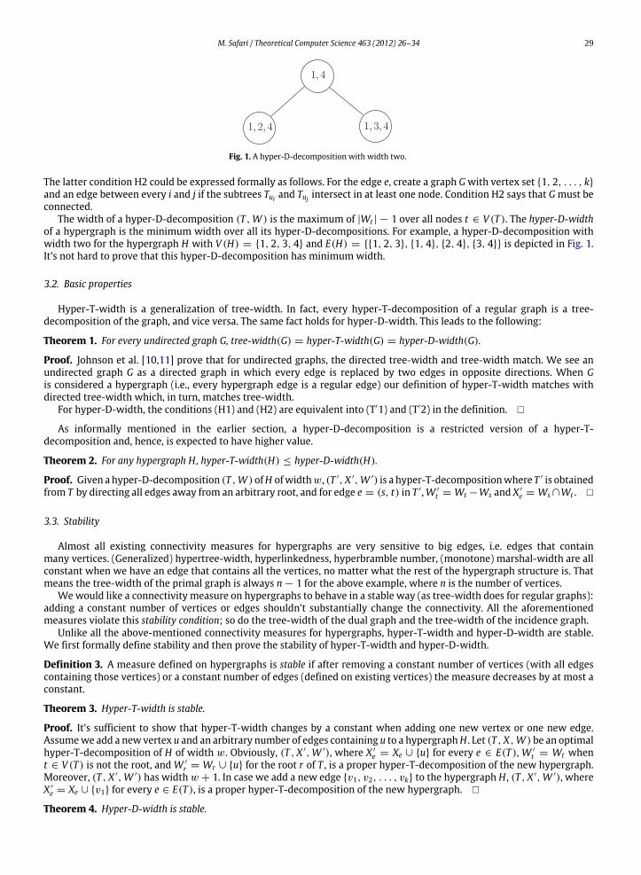
Fig. 1. A hyper-D-decomposition with width two.

The latter condition H2 could be expressed formally as follows. For the edge e, create a graph Gwith vertex set {1, 2, . . . , k}and an edge between every i and j if the subtrees Tui and Tuj intersect in at least one node. Condition H2 says that Gmust beconnected.

The width of a hyper-D-decomposition (T ,W ) is the maximum of |Wt | − 1 over all nodes t ∈ V (T ). The hyper-D-widthof a hypergraph is the minimum width over all its hyper-D-decompositions. For example, a hyper-D-decomposition withwidth two for the hypergraph H with V (H) = {1, 2, 3, 4} and E(H) = {{1, 2, 3}, {1, 4}, {2, 4}, {3, 4}} is depicted in Fig. 1.It’s not hard to prove that this hyper-D-decomposition has minimum width.

3.2. Basic properties

Hyper-T-width is a generalization of tree-width. In fact, every hyper-T-decomposition of a regular graph is a tree-decomposition of the graph, and vice versa. The same fact holds for hyper-D-width. This leads to the following:

Theorem 1. For every undirected graph G, tree-width(G) = hyper-T-width(G) = hyper-D-width(G).

Proof. Johnson et al. [10,11] prove that for undirected graphs, the directed tree-width and tree-width match. We see anundirected graph G as a directed graph in which every edge is replaced by two edges in opposite directions. When Gis considered a hypergraph (i.e., every hypergraph edge is a regular edge) our definition of hyper-T-width matches withdirected tree-width which, in turn, matches tree-width.

For hyper-D-width, the conditions (H1) and (H2) are equivalent into (T′1) and (T′2) in the definition. �

As informally mentioned in the earlier section, a hyper-D-decomposition is a restricted version of a hyper-T-decomposition and, hence, is expected to have higher value.

Theorem 2. For any hypergraph H, hyper-T-width(H) ≤ hyper-D-width(H).

Proof. Given a hyper-D-decomposition (T ,W ) ofH ofwidthw, (T ′, X ′,W ′) is a hyper-T-decompositionwhere T ′ is obtainedfrom T by directing all edges away from an arbitrary root, and for edge e = (s, t) in T ′,W ′

t = Wt −Ws and X ′e = Ws ∩Wt . �

3.3. Stability

Almost all existing connectivity measures for hypergraphs are very sensitive to big edges, i.e. edges that containmany vertices. (Generalized) hypertree-width, hyperlinkedness, hyperbramble number, (monotone) marshal-width are allconstant when we have an edge that contains all the vertices, no matter what the rest of the hypergraph structure is. Thatmeans the tree-width of the primal graph is always n − 1 for the above example, where n is the number of vertices.

We would like a connectivity measure on hypergraphs to behave in a stable way (as tree-width does for regular graphs):adding a constant number of vertices or edges shouldn’t substantially change the connectivity. All the aforementionedmeasures violate this stability condition; so do the tree-width of the dual graph and the tree-width of the incidence graph.

Unlike all the above-mentioned connectivity measures for hypergraphs, hyper-T-width and hyper-D-width are stable.We first formally define stability and then prove the stability of hyper-T-width and hyper-D-width.

Definition 3. A measure defined on hypergraphs is stable if after removing a constant number of vertices (with all edgescontaining those vertices) or a constant number of edges (defined on existing vertices) the measure decreases by at most aconstant.

Theorem 3. Hyper-T-width is stable.

Proof. It’s sufficient to show that hyper-T-width changes by a constant when adding one new vertex or one new edge.Assumewe add a new vertex u and an arbitrary number of edges containing u to a hypergraphH . Let (T , X,W ) be an optimalhyper-T-decomposition of H of width w. Obviously, (T , X ′,W ′), where X ′

e = Xe ∪ {u} for every e ∈ E(T ), W ′t = Wt when

t ∈ V (T ) is not the root, and W ′r = Wr ∪ {u} for the root r of T , is a proper hyper-T-decomposition of the new hypergraph.

Moreover, (T , X ′,W ′) has width w + 1. In case we add a new edge {v1, v2, . . . , vk} to the hypergraph H , (T , X ′,W ′), whereX ′e = Xe ∪ {v1} for every e ∈ E(T ), is a proper hyper-T-decomposition of the new hypergraph. �

Theorem 4. Hyper-D-width is stable.

30 M. Safari / Theoretical Computer Science 463 (2012) 26–34

Proof. It’s sufficient to show that hyper-D-width changes by a constant when adding one new vertex or one new edge.Assume we add a new vertex u and an arbitrary number of edges containing u to a hypergraph H . Let (T ,W ) be an optimalhyper-D-decomposition of H with width w. Obviously, (T ,W ′), whereW ′

t = Wt ∪{u} for every t ∈ V (T ), is a proper hyper-D-decomposition of the new hypergraph with widthw+1. In case we add a new edge {v1, v2, . . . , vk} to the hypergraph H ,(T ,W ′), where W ′

t = Wt ∪ {v1} for every t ∈ V (T ), is a proper hyper-D-decomposition of the new hypergraph with widthw + 1. �

In contrast, all the existing alternative measures are unstable.Theorem 5 (Generalized). Hypertree-width, hyperlinkedness, hyperbramble number, (monotone) marshal-width, (dual, inci-dence, or primal) tree width are all unstable.Proof. The first four parameters are within a constant factor of each other [1]. Hence it suffices to prove hypertree-widthand (dual, incidence, primal) tree width are unstable. LetH be a hypergraphwith big hypertree-width. Adding one edge thatcontains all the vertices makes the hypertree-width equal to one. Thus, hypertree-width is unstable. Similarly, the primaltree width is unstable. Now, let H be a hypergraph with small dual tree-width. Let H ′ be obtained from H by adding a newvertex u and all possible edges that contain u (i.e. 2n edges where n is the number of vertices). The dual graph of H ′ has aclique of size 2n (all edges that contain u) whichmeans it has dual tree-width at least 2n

−1, which shows dual tree-width isunstable (under removal of vertex u). As for the incidence graph supposeH is a hypergraphwith small incidence tree-width.We show thatH ′, as constructed above, has large incidence tree-width. Let I be the first n

2 vertices ofH . The number of edgesin H ′ that contain all vertices in I is at least 2

n2 which means the incidence graph of H ′ contains a K n

2 , n2(actually K n

2 ,2n2as

well) subgraph. Hence, its tree-width is at least n2 . �

3.4. Comparison

In this section we compare hyper-T-width and hyper-D-width with other existing parameters defined on hypergraphs,namely, the tree-width of the primal, dual, and incidence graph and we show that both hyper-T-width and hyper-D-widthare generally smaller values. As hyper-T-width is smaller than hyper-D-width (by Theorem 2), we only need to show thisfor hyper-D-width.Theorem 6. For any hypergraph H,

hyper-D-width (H) ≤ primal tree-width (H),hyper-D-width (H) ≤ incidence tree-width (H), andhyper-D-width (H) ≤ dual tree-width (H) + 1.

Proof. The first inequality follows from the fact that every tree-decomposition of the primal graph is a hyper-D-decomposi-tion. However, there exist hypergraphs with primal tree-width n − 1 and hyper-D-width one (a hypergraph with one edgecontaining all the vertices).

As for the incidence tree width, let (T ,W ) be a tree-decomposition of the incidence graph. For each edge e = {v1,v2, . . . , vk}, replace every occurrence of e in Wt for t ∈ V (T ) with v1. Since e and v1 share some node of T , i.e. {e, v1} ⊆ Wtfor some t ∈ V (T ), the nodes that contain v1 still make a connected subtree. Moreover, since e shares some node withevery vi, 1 ≤ i ≤ k, the vertices v1, v2, . . . , vk make a connected subtree in the resulting tree-decomposition. Again, thereare hypergraphs with small hyper-D-width, but large incidence tree-width. Assume H has 2n vertices {1, 2, . . . , 2n} and nedges of the form ei = {1, 2, . . . , n, n + i} for 1 ≤ i ≤ n. The incidence graph has a Kn,n subgraph (every i is connected toej for 1 ≤ i, j ≤ n) and, hence, has tree-width at least n. However, its hyper-D-width is one. Its minimum width hyper-D-decomposition is a star with root r containingWr = {1} and ith leaf containingWi = {1, i} for 2 ≤ i ≤ 2n.

Almost the same statement holds when comparing the dual tree-width and hyper-D-width. Given a tree-decomposition(T ,W ) with width w of the dual graph of hypergraph H , we show how a hyper-D-decomposition of H with width at mostw + 1 can be constructed.2 For any vertex u ∈ V (H), all edges that contain u make a clique in the dual graph. Hence,there is some node in T , say λ(u), that contains all such edges. In the first step, for all u ∈ V (H) we add a leaf l(u) withWl(u) = Wλ(u) ∪ {u} and attach it to the node λ(u) in T . Next, for every edge e ∈ E(H), we pick an arbitrary vertex v ∈ e andreplace e with v in every Wt for t ∈ V (T ). Call the resulting decomposition (T ′,W ′). Now, (T ′,W ′) contains only verticesof H . We claim that (T ′,W ′) is a hyper-D-decomposition of H . First, the new leaves ensure that every vertex u ∈ V (H) iscontained in someWt (in particular,Wl(u)) in T ′. Second, for any vertex u ∈ V (H), all nodes t ∈ V (T ′) such that u ∈ W ′

t makea connected subtree. Every edge e replaced by u in creating T ′, forms a connected subtree in T that contains the node λ(u).Hence, these subtrees are connected in T ′ and they connect to the new leaf node l(u). Third, suppose e = {x1, x2, . . . , xk}is replaced by x1, then T ′

|x1 ∩ T ′|xj = ∅. In fact, λ(xj) ∈ T ′

|x1 ∩ T ′|xj . So the subtrees corresponding to vertices of e form

a connected subtree. This bound is, however, not tight, as a star graph of size n has tree-width one and (by Theorem 1)hyper-D-width one whereas its dual graph is a clique and, hence, has tree-width n − 1. �

2 On regular graphs we can remove the additive constant one in the inequality.

M. Safari / Theoretical Computer Science 463 (2012) 26–34 31

Corollary 1. The class of bounded hyper-T-width (hyper-D-width) hypergraphs contains the class of bounded (primal, dual, orincidence) hypergraphs.

As for comparing hyper-T-width with hypertree-width, the two are, in fact, not comparable. The hypertree-width of anhypergraphwith one edge containing all the vertices is onewhereas its hyper-T-width can be large. Thatmeans a hypergraphin which every edge contains a common vertex has hyper-T-width one whereas its hypertree-width can be large. However,if the edges in a hypergraph have constant size then the hypertree-width and primal tree-width are within a constant factorof each other and, hence, in this case, hyper-T-width is a lower bound for hypertree-width up to a constant factor. The samestatements hold for hyper-D-width.

3.5. Computation

The big advantage of hyper-T-width over hyper-D-width is the fact that we can approximate it within a constant factor.Johnson et al. [10] prove this for directed tree-width and their proof translates immediately to hypergraphs.

The details of how this result transfers to hypergraphs is moved to Section 5 for ease of presentation.

Computing hyper-D-widthAlthough hyper-D-width has several nice properties and resembles undirected tree-width in a natural way, it has one big

disadvantage:We don’t know a polynomial time algorithm for computing optimal or even approximately (within a constantfactor).

It’s worthmentioning that existing separator-based algorithms for computing tree-decompositions of undirected graphscannot be easily used for hyper-D-decomposition. These algorithms find a good separator X , break the input graph intoconnected components C1, C2, . . . , Cm, find good tree-decompositions Ti for every part X ∪ Ci (such that X appears entirelyin some node) and then combine these tree-decompositions through the nodes that contain X . As every edge of the originalgraph exists in at least one of the parts X ∪ Ci, the combination process guarantees that the new tree-decomposition is afeasible one for the original graph.

Such a thing, however, cannot be guaranteed for hypergraphs. Unless we introduce new edges in partitions, there mightbe some edges in the original hypergraph that do not exist in any of the partitions and, therefore, the combination processwould not necessarily create a feasible hyper-D-decomposition. Adding these edges (andmaking sure at the same time thatit would not substantially increase the hyper-D-width) does not seem to be an easy task.

We can, however, use the balanced-separator property of hyper-D-width and obtain an O(log n)-factor approximationfor constant hyper-D-width hypergraphs. Similar to regular tree-width, a hyper-D-decomposition of small width implies asmall balanced separator:

Theorem 7. For every hypergraph H of hyper-D-width w and any subset S ⊆ V (H), there exists a subset X ⊆ V (H) of at mostw + 1 vertices such that every connected component of H\X contains at most |S|

2 vertices from S.

Proof. The proof is essentially the same as the one for regular tree-width. Given a hyper-D-decomposition (T ,W ) ofH withwidth w, let t be the deepest node (pick an arbitrary node as the root) such that the sub-tree rooted at t has at least |S|

2vertices from S. Every connected component of H\Wt has at most |S|

2 vertices from S, henceWt is the desired separator. �

The balanced separator property can be used, for example, to compute an O(log n)-approximation for hyper-D-width.

Theorem 8. There exist an O(log n)-factor approximation algorithm for computing hyper-D-width when it is constant.

Proof. Let hypergraph H with n vertices have hyper-D-widthw. Then, for any subset S ⊆ V (H), there exists a set X ⊆ V (H)

of size at most w + 1 such that every connected component of H\X has at most |S|2 of vertices of S. Finding such a subset

X for S = V (H) takes polynomial time (for constant w). Let C1, C2, . . . , Ck be the components of H\X and let (T i,W i) be arecursively computed hyper-D-decomposition for Ci. The hyper-D-decomposition (T ,W ) of H is computed as follows. T isobtained by making a new node r and connecting it to one arbitrary node from each T i. Wr = X and for any node t ∈ T i,Wt = W i

t ∪ X . It’s easy to see that (T ,W ) is a hyper-D-decomposition of H . If (T i,W i) is a hyper-D-decomposition for Ciwith width at most (lg |Ci| + 1)(wi + 1) − 1 where wi is the optimal width, since |Ci| ≤ |S|/2 and wi < w, the addition ofX to eachW i

t creates a setWt of size at most (lg |Ci| + 1)(wi + 1) + (w + 1) which is at most (lg n + 1)(w + 1). Hence, theresult is an O(log n) approximation.

One can prove by induction that the running time of the algorithm is at most O(mnw+3), wherem is the number of edgesin the hypergraph and n is the number of vertices. For finding a good separator X , we can try all possible O(nw+2) sets ofsize at most w + 1 and verify if they are good separators in time O(nm). The recursive time is dominated by the time takenby finding good separators. �

4. Applications

In this section we show that there exist polynomial-time approximation schemes (PTAS) for many hard problemsincluding vertex cover, dominating set, and multicut problems on hypergraphs when the hyper-T-width of the inputhypergraph is constant. In other words, these problems admit FP-approximation schemes.

32 M. Safari / Theoretical Computer Science 463 (2012) 26–34

In the minimum vertex cover problem, we want to choose the minimum number of vertices such that at least one vertexfrom each edge is chosen. In the minimum dominating set problem we want to choose the minimum number of verticessuch that each vertex is either chosen or at least one of its neighbors is chosen. Finally, in the vertex multicut problem thereare k pairs (si, ti), i = 1, 2, . . . , k given, and our goal is to choose the minimum number of vertices X such that all the pairsare separated, i.e. no two si and ti are within the same connected component of H\X .

A vertexminimization problem on hypergraphs is of the form: given a hypergraphH , find theminimumnumber of verticesin H that together satisfy some property.

We are especially interested in vertex minimization problems P with the following decomposability property. For anysubset S of vertices of H , let C1, C2, . . . , Cm be the connected components of H\S. Let Di be a solution for P on H[Ci]. Then,S ∪ (D1 ∪ D2 ∪ · · · ∪ Dm) is a feasible solution (not necessarily optimal) of P on H .

The decomposability property lets us choose any suitable S, put it in the solution, break the input hypergraph into smallerparts, and solve the problem on each part independently. It’s easy to verify that multicut, dominating set, and vertex coverare examples of such problems. For example, for the vertex cover problem, if we choose all vertices in S then any edge thatintersects both Ci and Cj (i = j) or both Ci and S is covered as such an edge must contain a vertex in S. The rest is, then,solving the vertex cover problem on each Ci separately.

Now, we show how such problems have a PTAS on bounded hyper-T-width hypergraphs. The idea is similar to thetechnique that Calinescu et al. [4] use to find a PTAS for multicut on bounded tree-width graphs and digraphs. Let (T , X,W )be a hyper-T-decomposition with widthw for the input hypergraph. Let t ∈ V (T ) be the deepest node such that there existsan optimal global solution that contains at least w/ϵ vertices inW (Tt) :=

s∈Tt Ws where Tt is the subtree of T rooted at t .

If there is no such t then the optimal global solution has fewer than w/ϵ vertices. Such a solution can be computed in timeO(nw/ϵ). Otherwise, let opt t be the number of vertices of an optimal solution inW (Tt). Choosing and removing all vertices inλt = Wt ∪

e∼t Xe breaks H[W (Tt)] into several connected components each having less than w/ϵ vertices of the optimal

solution. Hence, the problem can be solved by brute force on all these components in time O(nw/ϵ). Hence, the number ofvertices that we pick is at most opt t + w ≤ opt t(1 + ϵ). Assume that the rest of the hypergraph has opt vertices in theoptimal solution. According to the induction hypothesis, we can find a solution with at most opt(1 + ϵ) vertices. Hence,we can solve the problem on H by choosing at most (1 + ϵ)(opt t + opt) vertices, yielding a (1 + ϵ)-factor approximationfor P . The details of the algorithm are shown in Algorithm 1. As we perform the recursive step at most O(n) times, the totalrunning time is in O(n1+w/ϵ).

Input: A hypergraph H together with an optimal hyper-T-decomposition (T , X,W ) of width w.Output: Set of vertices that satisfies P and is at most 1 + ϵ times bigger than the smallest such set.

1 foreach t ∈ V (T ) do2 Let ti, i = 1, 2, . . . ,m, be children of t .3 foreach i do4 Find an optimal solution OPT i to P of size at most w/ϵ for H[W (Tti) − λt ]. If no such solution exists then try the

next t .5 end6 Let OPT = ∪iOPT i.7 Recursively find a (1 + ϵ)-factor approximation solution S ′ for H\(W (Tt) ∪ λt) with hyper-T-decomposition

(T\Tt , X,W ′) where W ′t = Wt − W (Tt).

8 Let St = OPT ∪ S ′∪ λt .

9 end10 Return St with minimum size.

Algorithm 1: Approximately solving decomposability problem P on a hypergraph whose hyper-T-width is w.

To complete this section we prove that all aforementioned problems are hard even on bounded hyper-D-width hyper-graphs. Remember that hyper-D-width is an upper bound for hyper-T-width and, therefore, the hardness applies to boundedhyper-T-width graphs as well.

Theorem 9. The vertex cover problem, the dominating set problem, and themulticut problem areNP-complete on bounded hyper-D-width hypergraphs.

Proof. Let C1, C2, . . . , Cm be a SAT problem instance over variables x1, x2, . . . , xn. We make a hypergraph H with vertexset V (H) = {u} ∪

1≤i≤n {xi, xi, zi} and edge set E(H) = {Ci ∪ {u}|1 ≤ i ≤ m} ∪ {{xi, xi, zi}|1 ≤ i ≤ n}. We claim that

the SAT problem instance is satisfiable if and only if the hypergraph H has a vertex cover of size exactly n. Assume theSAT instance is satisfiable with setting all xi’s in a set X to be true and the rest to be false. In the hypergraph let the vertexcover be X ∪ {xi|xi ∈ X}. Every edge of type Ci ∪ {u} and every edge of type {xi, xi, zi} is covered and the size of the vertexcover is n. On the other hand, let X be a vertex cover of size at most n. It must contain exactly one vertex from every triple{xi, xi, zi}, 1 ≤ i ≤ n. Moreover, every edge of type Ci ∪ {u} must be covered by some xi or xi in Ci, which makes a satisfiablesolution. Finally, we mention that the hypergraph constructed above has hyper-D-width at most three. A star whose root rhasWr = {u} and whose ith leaf hasWi = {u, xi, xi, zi}, for 1 ≤ i ≤ n is a hyper-D-decomposition of width 3.

M. Safari / Theoretical Computer Science 463 (2012) 26–34 33

a

b

c de

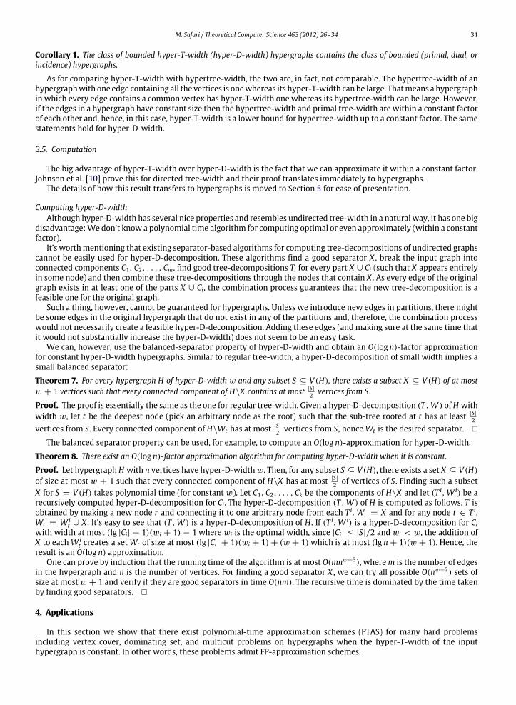
Fig. 2. A graph with haven order 2.

It’s easy to prove that the above reduction works for the dominating set problem as well. The NP-completeness of themulticut problem follows from its NP-completeness on bounded tree-width graphs proven by Calinescu et al. [4]. �

5. Computing hyper-T-width

We basically mimic the proof for computing directed tree-width of Johnson et al. [10] here. As our definitions ofconnectivity and havens are different from theirs, the proof is outlined below.

Recall the following definitions from [10,11].

Definition 4 (Arboreal (pre-)decompositions and directed tree-width). An arboreal pre- decomposition of a digraph G is atuple (T , X,W ) where T is an arborescence and W = (Wt |t ∈ V (T )) and X = (Xe|e ∈ E(T )) are families of subsets of V (G)that satisfy:

(A1) W is a partition of V (G) into (possibly empty) sets such thatWr = ∅ for the root r of T , and(A2) If e ∈ E(T ), then

t>e Wt is Xe-normal or empty.

Thewidth of an arboreal pre-decomposition (T , X,W ) is the minimum k such that for all t ∈ V (T ), |Wt ∪

e∼t Xe| ≤ k+ 1.An arboreal decomposition is a pre-decomposition in which allWt are non-empty, and the directed tree-width of a digraph Gis the minimal width of all its arboreal decompositions.

According to Johnson et al. [10] a set S is Z-normal if every path from a vertex in S to another vertex in S that containsa vertex in V (G) − S has a vertex in Z as well. That means there is no strongly connected component of G\Z that containsvertices from both S and V (D) − S.

Let’s now define haven order on hypergraphs.

Definition 5 (Haven and Haven-order). Let H be a hypergraph. A haven of order k is a function β assigning to every setZ ⊆ V (H) with |Z | < k, a connected component of H \ Z such that if X ⊆ Y ⊆ V (H) and |Y | < k then β(Y ) ⊆ β(X). Thehaven-order of H is the largest k such that H has a haven of order k.

The graph in Fig. 2 has haven order 2 as β(Z) = {a, b, c}\Z is a haven and it also cannot have a haven of order 3 for thefollowing reason. Let β be a haven of order 3. Without loss of generality assume β({a, c, d}) = {b}. So, β({a, c}) = {b} andβ({a, b, c}) = {d, e} which is a contradiction given that {a, c} ⊂ {a, b, c}.

Theorem 10. H(H) − 1 ≤ hyper-T-width(H) ≤ 3H(H) + 1 for hypergraphs H, where H(H) is the haven order of H.

Proof. (Left inequality)The proof is identical to the corresponding proof of Johnson et al. [10] for directed tree-width.(Right inequality) Assume H has no haven of order w. First, let’s prove the following crucial lemma.

Lemma 1. If H has no haven of order w then for every set Y of vertices of H with |Y | ≤ 2w − 1 there is a subset Z of vertices ofH such that |Z | < w and every connected component of H\Z has at most w − 1 vertices of Y .

Proof. Assume not. Then for every set Z with |Z | < w there is one connected component ofH\Z , say β(Z), such that |β(Z)∩Y | ≥ w. But, this is a contradiction as β is a haven of orderw. For any Z and Z ′ with Z ⊂ Z ′ and |Z ′

| < w, both β(Z) and β(Z ′)contain at least w vertices from Y . As |Y | ≤ 2w − 1, we conclude that β(Z) ∩ β(Z ′) = ∅ which means β(Z ′) ⊆ β(Z). �

Consider a hyper-T-decomposition (T , X,W ) of H with the following restrictions.

1. For any node r , if r is not a leaf then |Wr | ≤ w and |λr | ≤ 3w − 1.2. For any edge e, |Xe| ≤ 2w − 1.3. Subject to the above conditions we take the hyper-T-decomposition that minimizes the maximum of |Wr |, for all r ’s.

34 M. Safari / Theoretical Computer Science 463 (2012) 26–34

As the obvious hyper-T-decomposition with one vertex r andWr = V (H) satisfies the first two conditions, we concludethat there exists a hyper-T-decomposition (T , X,W ) satisfying the above three conditions. If there is no leaf with |Wr | > rthen we are done and (T , X,W ) would have width at most 3w − 2. Otherwise, take the leaf r with maximum |Wr |. Assumer ′ is the unique parent of r , e = (r ′, r) and Y = Xe. According to Lemma 1 there exists a set Z0 of at most w − 1 vertices of Hsuch that every connected component of H\Z0 contains at most w − 1 vertices from Y . Let Z = Z ∪ {u} for some arbitraryvertex u in Wr . We build a new hyper-T-decomposition satisfying the first two conditions, but a smaller |Wr | which is acontradiction.

Let C1, C2, . . . , Cm be the connected components of H[Wr ]\Z . We create m new leaves r1, r2, . . . , rm and connect themto r (i.e. create edges from r to each ri). SetWri = Ci and changeWr to Z ∩Wr . For the edge ei = (r, ri) set Xei = Z ∪ (Y ∩ Ci).As |Y ∩ Ci| ≤ 2w − 1 this insures that |Xei | satisfies condition 2. By the way, λr = Z ∪ Y ; thus, |λr | ≤ 3w − 1. �

The proof that hyper-T-width(H) ≤ 3H(H) + 1 is constructive and can be used to obtain an approximate hyper-T-decomposition. There is at most n optimization steps during whichwe find a set Z and add new leaves to the existing hyper-T-decomposition. Finding a set Z of size less than w and verifying that all connected components H\Z contain less than wvertices of Y can be done in time O(nw+2). Hence the total running time for finding an approximate hyper-T-decompositionwould be O(nw+3).

6. Conclusion

Hyper-T-width and hyper-D-width are very new and there exist several open problems related to them. An efficientalgorithm for computing optimal (or constant-factor approximate) hyper-D-decompositions for small hyper-D-widthwouldbe very useful. Exploring algorithmic aspects of hyper-D-width and hyper-T-width is also a very interesting researchdirection.

Another interesting direction is exploring a set of problems in which the notion of connectivity matches with what weadopt here. There are some fundamental problems (such as solving CSP, SAT, and finding Nash equilibria of certain games)that seem to be relevant to hyper-D-width and hyper-T-width and finding those connections is an interesting problem.

For example, in certain game theory settings, the utility of players depend on an all-or-nothing basis. One concurrentsuch example is a setting in combinatorial auctions (called single-minded) in which each player i has a set Wi of goods andhe either wants nothing or all goods in Si and a sample work [3] on proving hardness results to compute even fundamentalconcepts such as Walrasian equilibrium.

In the SAT problem, an edge corresponds to a clause and, again, carries an all-or-nothing type of information and isrelevant to our view of connectivity in the sense that when you pick a node (satisfy a variable) all clauses in it would besatisfied and, hence, you can safely remove them. In a similar way, certain CSP problems might be easy to deal with whenwe consider hyper-T-width and hyper-D-width.

Acknowledgments

I would like to thankWill Evans and anonymous reviewers for theirmany valuable comments throughout the preparationof this paper.

References

[1] Isolde Adler, Georg Gottlob, Martin Grohe, Hypertree-width and related hypergraph invariants, in: Stefan Felsner (Ed.), 2005 European Conference onCombinatorics, Graph Theory and Applications (EuroComb’05), volumeAE of DMTCS Proceedings, in: DiscreteMathematics and Theoretical ComputerScience, 2005, pp. 5–10.

[2] S. Arnborg, J. Lagergren, D. Seese, Easy problems for tree-decomposable graphs, Journal of Algorithms 12 (2) (1991) 308–340.[3] Ning Chen, A Xiaotie Deng, C. Xiaoming Sun, On complexity of single-minded auction, Journal of Computer and System Sciences 69 (2004) 675–687.[4] Gruia Calinescu, Cristina G. Fernandes, Bruce Reed, Multicuts in unweighted graphs and digraphs with bounded degree and bounded tree-width,

Journal of Algorithms 48 (2) (2003) 333–359.[5] Liming Cai, XiuzhenHuang, Fixed-parameter approximation: Conceptual framework and approximability results, Algorithmica 57 (2) (2010) 398–412.[6] R.G. Downey, M.R. Fellows, Fixed-parameter intractability, in: Proceedings of the 7th Annual Conference on Structure in Complexity Theory, 1992,

pp. 36–49.[7] Georg Gottlob, Martin Grohe, Nysret Musliu, Marko Samer, Francesco Scarcello, Hypertree decompositions: Structure, algorithms, and applications,

in: Dieter Kratsch (Ed.), Proceedings of the 31st International Workshop on Graph-Theoretic Concepts in Computer Science, WG05, in: Lecture Notesin Computer Science, volume 3787, Springer-Verlag, Berlin Heidelberg, 2005, pp. 1–15.

[8] Georg Gottlob, Nicola Leone, Francesco Scarcello, Hypertree decompositions and tractable queries, Journal of Computer and System Sciences 209(2002) 1–45.

[9] Georg Gottlob, Zoltan Miklos, Thomas Schwentick, Generalized hypertree decompositions: np-hardness and tractable variants, in: PODS’07:Proceedings of the twenty-sixth ACM SIGMOD-SIGACT-SIGART symposium on Principles of database systems, ACM, New York, NY, USA, 2007,pp. 13–22.

[10] T. Johnson, N. Robertson, P.D. Seymour, R. Thomas, Directed tree-width, Journal of Combinatorial Theory (Series B) 82 (2001) 128–154.[11] T. Johnson, N. Robertson, P.D. Seymour, R. Thomas, Addendum to Directed Tree-Width. manuscript, 2002.