Hypersurface Normalizations and Numerical Invariants

by Brian Hepler

B.A. in Mathematics, Boston UniversityM.S. in Mathematics, Northeastern University

A dissertation submitted to

The Faculty ofthe College of Science ofNortheastern University

in partial fulfillment of the requirementsfor the degree of Doctor of Philosophy

April 12th, 2019

Dissertation directed by

David B. MasseyProfessor of Mathematics

1

Acknowledgements

I would like to acknowledge the mathematics department at Northeastern University for

many years of engaging discussion and opportunities for mathematical and personal growth.

In particular, I would like to thank all of the graduate students, current and former, without

whose unwavering support and encouragement I would not be here to write this dissertation:

Nathaniel Bade, Antoni Rangachev, Barbara Bolognese, Floran Kacaku, Simone Cecchini,

Gourishankar Seal, Jose Simental-Rodriguez, Rahul Singh, and Saif Sultan.

I would like to more directly thank Antoni Rangachev and Rahul Singh for many discus-

sions on singularities and algebraic geometry; one day, I hope to understand what you are

talking about.

I would like to thank Jorg Schurmann for answering my many questions on Hodge the-

ory and D-modules, and in particular suggesting simplifications to the proofs of Proposi-

tion 3.2.0.5 and Theorem 3.2.0.6.

I would like to thank Terence Gaffney for many discussions, support, and advice over the

years. I am slowly coming to understand singularities of mappings. He originally suggested

the interpretation that one should think of parameterizing a hypersurface in terms of the

normalization, which ultimately led to Theorem 1.1.1.4 and the statement of Theorem 2.4.0.2

in terms of rational homology manifolds. In addition to discussions leading to the statement

of Theorem 2.4.0.7, Terry has also provided numerous interesting applications to his own

work (e.g., Remark 2.4.0.11) and future directions to pursue.

I don’t think I can quite thank David Massey enough; everything I know about the

derived category and perverse sheaves and singularities is due to him. He has helped me

grow a mathematician and as a person over my long years in graduate school. I expect us

to remain lifelong collaborators and friends in the years to come.

Finally, I thank my family and girlfriend, Fatema Abdurrob, for keeping me alive and

for their endless support and love. I would not be here without you.

2

Abstract of Dissertation

We define a new perverse sheaf, the comparison complex, naturally associated to any

locally reduced complex analytic space X on which the (shifted) constant sheaf Q•X [dimX]

is perverse. In the hypersurface case, this complex is isomorphic to the perverse eigenspace

of the eigenvalue one for the Milnor monodromy action on the vanishing cycles; we also

examine how the characteristic polar multiplicities of this complex behave in certain one-

parameter families of deformations of hypersurfaces with codimension-one singularities, and

generalize a classical formula for the Milnor number of a plane curve singularities in terms

of double-points. In general, the vanishing of the cohomology sheaves of the comparison

complex provide a criterion for determining if the normalization of the space X is a rational

homology manifold. When the normalization is a rational homology manifold, we can also

compute several terms in the weight filtration of the constant sheaf Q•X [dimX] in those

cases for which this perverse sheaf underlies a mixed Hodge module. In the surface case

V (f) ⊆ C3, this produces a new numerical invariant, the weight zero part of the constant

sheaf, which is a perverse sheaf concentrated on a single point.

We then prove two special cases of a conjecture of Javier Fernandez de Bobadilla for

hypersurfaces with 1-dimensional critical loci (Corollary 4.2.0.2 and Theorem 4.3.0.2). We

do this via a new numerical invariant for such hypersurfaces, called the beta invariant, first

defined and explored by the Massey in 2014. The beta invariant is an algebraically calculable

invariant of the local ambient topological-type of the hypersurface, and the vanishing of

the beta invariant is equivalent to the hypotheses of Bobadilla’s conjecture. Bobadilla’s

Conjecture is related to a more well-known conjecture by Le Dung Trang (Conjecture 4.0.0.1)

regarding the equsingularity of parameterized surfaces in C3.

3

Table of Contents

Acknowledgments 2

Abstract of Dissertation 3

Table of Contents 4

Disclaimer 6

Introduction 7

1 Parameterized Spaces 11

1.1 The Fundamental Short Exact Sequence . . . . . . . . . . . . . . . . . . . . . . 11

1.1.1 The Fundamental Short Exact Sequence and The Normalization . . . . . . . . 12

1.1.2 A Trivial, Non-Trivial Example . . . . . . . . . . . . . . . . . . . . . . . . . . 17

1.2 Parameterized Hypersurfaces . . . . . . . . . . . . . . . . . . . . . . . . . . . . 20

1.3 Milnor Fibers in Parameterized Spaces . . . . . . . . . . . . . . . . . . . . . . . 21

1.3.1 Functions with Arbitrary Singularities . . . . . . . . . . . . . . . . . . . . . . 22

1.3.2 Functions with Isolated Singularities . . . . . . . . . . . . . . . . . . . . . . . 26

2 Generalizing Milnor’s Formula to Higher Dimensions 29

2.1 IPA-Deformations . . . . . . . . . . . . . . . . . . . . . . . . . . . . . . . . . . . 31

2.2 Unfoldings and N•V (f) . . . . . . . . . . . . . . . . . . . . . . . . . . . . . . . . . 38

2.3 Characteristic Polar Multiplicities . . . . . . . . . . . . . . . . . . . . . . . . . . 40

2.4 Milnor’s Result and Beyond . . . . . . . . . . . . . . . . . . . . . . . . . . . . . 46

3 Some Hodge Theoretic Aspects of Parameterized Spaces 56

3.1 Introduction . . . . . . . . . . . . . . . . . . . . . . . . . . . . . . . . . . . . . . 58

3.2 General Case for Parameterized Spaces . . . . . . . . . . . . . . . . . . . . . . . 60

4

3.3 The Weight Zero Part in the Surface Case . . . . . . . . . . . . . . . . . . . . . 67

3.3.1 Interpretation via Invariant Jordan Blocks of the Monodromy . . . . . . . . . 70

3.4 Connection with the Vanishing Cycles . . . . . . . . . . . . . . . . . . . . . . . 71

3.5 The Algebraic Setting and Saito’s Work . . . . . . . . . . . . . . . . . . . . . . 72

4 Bobadilla’s Conjecture and the Beta Invariant 74

4.1 Bobadilla’s Conjecture . . . . . . . . . . . . . . . . . . . . . . . . . . . . . . . . 75

4.2 Generalized Suspension . . . . . . . . . . . . . . . . . . . . . . . . . . . . . . . . 79

4.3 Γ1f,z0

as a hypersurface in Γ2f,z . . . . . . . . . . . . . . . . . . . . . . . . . . . . 80

4.3.1 Non-reduced Plane Curves . . . . . . . . . . . . . . . . . . . . . . . . . . . . . 86

A The Le Cycles and Relative Polar Varieties 89

B Singularities of Maps 91

Bibliography 93

5

Disclaimer

I hereby declare that the work in this thesis is that of the candidate alone, except where

indicated in the text, and as described below.

6

Introduction

The main focus of the author’s research is the local topology of complex analytic spaces

with arbitrary singularities. Largely, this research is concerned with the use of perverse

sheaves and derived category techniques in extending classical results for isolated singularities

in affine or projective space to arbitrarily singular complex analytic spaces.

The main object of study that threads together the work in this dissertation is a perverse

sheaf called the comparison complex, first defined by the author and David Massey in

[23] (where we originally referred to it as the multiple-point complex, for reasons that

will become clear in Formula 1.4), and subsequently studied in several papers by the author

in [20], [21], [22], and Massey in [39]. This perverse sheaf, denoted N•X , is defined on any

pure-dimensional (locally reduced) complex analytic space X for which the constant sheaf

Q•X [dimX] is perverse.

On such a space, there are two “fundamental” perverse sheaves: the constant sheaf

Q•X [dimX], and the intersection cohomology complex I•X with constant coefficients, with

a natural surjective map Q•X [dimX] → I•X → 0, where, in a certain sense, I•X detects the

singularities of X. Then, the comparison complex N•X “compares” these two complexes in a

manner analogous to the way the vanishing cycles compares the constant sheaf on a (possibly

singular) hypersurface V (f) with a nearby smooth fiber of f . The success of the vanishing

cycles in understanding the the topology of complex analytic spaces cannot be overstated,

and it is therefore natural to hope that N•X will have similarly wide application. The simplest

class of singular spaces we can analyze with N•X are those we call parameterized spaces.

7

For such spaces, we obtain a generalization of MIlnor’s classical formula for plane curve

singularities V (f0) ⊆ C2 in terms of double points appearing in a stable deformation µ0(f0) =

2δ − r + 1 (where δ is the number of double points, and r is the number of irreducible

components of V (f0) at 0). For higher-dimensional parameterized hypersurfaces V (f0), this

generalization is expressed in terms of the Le numbers of f0 and ft0 , and the characteristic

polar multiplicities of N•V (f0) and N•V (ft0 ):

λ0f0,z

(0) = −λ0N•V (f0)

,z(0) +∑

p∈Bε∩V (t−t0)

(λ0ft0 ,z

(p) + λ0N•V (ft0

),z(p)

).

While these numerical invariants allow us to compute information about these higher-

dimensional singluarities, they do also include contributions from points on the absolute

polar curve, which arise from the choice of coordinates (see Theorem 2.4.0.2 and Theo-

rem 2.4.0.7)

Throughout Chapter 1,2, and 3, we will be primarily concerned parameterized spaces

(Definition 1.1.1.7). These spaces are locally reduced, and have codimension-one singular-

ities. While this might normally make the topology of these spaces hard to analyze, our

approach using perverse sheaves allows us to make some headway. Particularly, these spaces

are interesting because (using Z coefficients) the constant sheaf Z•X [dimX] is perverse, and

intersection cohomology with constant coefficients is of the form I•X∼= π∗Z•X [dimX], where

Xπ−→ X is the normalization of X. With just these properties, we can conclude many things.

In Chapter 1, we introduce parameterized spaces, the fundamental short exact sequence

of perverse sheaves on X, and Theorem 1.1.1.4, which is our main criterion for determin-

ing if a space is parameterized. The main tool throughout this chapter is the comparison

complex N•X , a perverse sheaf naturally defined on any pure-dimensional, locally reduced

space, which has a particularly nice form for parameterized spaces (which we have also called

the multiple-point complex on such spaces). We conclude Chapter 1 by investigating Mil-

nor fibers of functions defined on parameterized spaces, and give formulas for computing the

8

cohomology of these Milnor fibers in terms of the (hyper)cohomology of the comparison com-

plex (Theorem 1.3.1.4). Using the techniques developed in Section 1.3, we first encounter and

re-prove Milnor’s formula for the Milnor number of a plane curve singularity in terms of the

number of double-points appearing in a stable deformation of the curve (Theorem 1.3.2.4).

The results from this chapter (unless otherwise specified) are from [21] by the author, and

[23] by the author and David Massey.

In Chapter 2, our main goal is to generalize Milnor’s formula (Theorem 1.3.2.4) to higher

dimensions using deformations of parameterized hypersurfaces V (f). To do this, we apply

the theory of deformations with isolated polar activity (IPA-deformations, Section 2.1,

originally developed by David Massey in [41]) as the “correct” way to deform a parameter-

ized space so that we can apply the same methods used in our proof of Milnor’s formula

from the curve case. The numerical invariants involved in this theory are the Le numbers

of the function defining the hypersurface V (f), and the characteristic polar multiplicities of

the comparison complex N•V (f), are the “correct” numbers to keep track of when deform-

ing parameterized hypersurfaces. Finally, in Section 2.4, we prove Theorem 2.4.0.2, which

generalizes Milnor’s theorem to deformations of parameterized hypersurfaces of arbitrary

dimension. We give particular examples of the formulas we obtain for deformations of pa-

rameterized surfaces in C3 in Theorem 2.4.0.7 and Corollary 2.4.0.8 . Such formulas exist

for deformations of parameterized hypersurfaces V (f) in Cn+1, provided we stay in Mather’s

“nice dimensions” n < 15. The results from this chapter (unless otherwise specified) are

from the preprint [20] by the author.

In Chapter 3, we investigate the question: “when is N•X a semi-simple perverse sheaf,

so that Q•X [n] is an extension of semi-simple perverse sheaves?” This question was posed

to us by a referee of [21], and led us to understand the structure of N•X as a mixed Hodge

module on X. It is well-known that, locally, Q•X [n] underlies a mixed Hodge module of

weight ≤ n on X, with weight n graded piece isomorphic to the intersection cohomology

9

complex I•X with constant Q coefficients. In this chapter we identify the weight n − 1

graded piece GrWn−1Q•X [n] in the case where X is a parameterized space (Theorem 3.2.0.6).

We then give concrete computations of the perverse sheaf W0Q•V (f)[2] in the case where

X = V (f) is a parameterized surface in C3 (Theorem 3.3.0.1). We conclude the chapter

with some connections to the work of David Massey regarding the eigenspaces of the Milnor

monodromy (Section 3.4), and the work of Morihiko Saito in the complex algebraic setting

(Section 3.5). The results from this chapter (unless otherwise specified) are from the preprint

[22] by the author.

In Chapter 4, we prove two special cases of a conjecture of Javier Fernandez de Bobadilla

for hypersurfaces with 1-dimensional critical loci (Corollary 4.2.0.2 and Theorem 4.3.0.2).

We do this via a new numerical invariant for such hypersurfaces, called the beta invariant,

first defined and explored by the Massey in 2014. The beta invariant is an algebraically cal-

culable invariant of the local, ambient topological-type of the hypersurface, and the vanishing

of the beta invariant is equivalent to the hypotheses of Bobadilla’s conjecture. Bobadilla’s

Conjecture is related to a more well-known conjecture by Le Dung Trang (Conjecture 4.0.0.1)

regarding the equsingularity of parameterized surfaces in C3, which was our original motiva-

tion for approaching Bobadilla’s Conjecture. The results from this chapter (unless otherwise

specified) are from the paper [24] by the author and David Massey.

10

Chapter 1

Parameterized Spaces

1.1 The Fundamental Short Exact Sequence

Let U be a connected open neighborhood of the origin in CN , and let X ⊆ U be a reduced

complex analytic space containing 0 of pure dimension n, on which the (shifted) constant

sheaf Z•X [n] is perverse (e.g., if X is a local complete intersection).

There is then a surjection of perverse sheaves Z•X [n] → I•X → 0, where I•X is the inter-

section cohomology complex on X with constant Z coefficients. This follows from the fact

that I•X is also the intermediate extension of the local system Z•X\ΣX [n] to all of X (where

ΣX denotes the singular locus of X), and therefore has no perverse quotient objects with

support contained in ΣX. Since Z•X [n]→ I•X is an isomorphism when restricted to X\ΣX,

the cokernel of this morphism is zero.

Remark 1.1.0.1. If one works with Q coefficients, Q•X [n] is still perverse, and I•X (with

Q coefficients) is a semi-simple object in the category of perverse sheaves on X with no

perverse sub or quotient objects with support contained in ΣX. Since the cokernel of the

natural morphism Q•X [n] → I•X has support contained in ΣX, the natural morphism must

be surjective.

11

Since the category of perverse sheaves on X is Abelian, there is a perverse sheaf N•X on

X such that

0→ N•X → Z•X [n]→ I•X → 0 (1.1)

is a short exact sequence of perverse sheaves. When Z•X [n] is perverse, this sheaf and I•X

are, essentially, the two fundamental perverse sheaves on X. For this reason, we make the

following definition.

Definition 1.1.0.2. We refer to (1.1) as the fundamental short exact sequence of X.

Definition 1.1.0.3. We refer to the perverse sheaf N•X as the comparison complex on

X.

The comparison complex was first defined and explored by the author and David Massey

in [23], and subsequently studied in several papers by the author [20],[21],[22] and Massey

[39]. The comparison complex N•X and the fundamental short exact sequence are the main

objects of study in Chapter 1, Chapter 2, and Chapter 3.

1.1.1 The Fundamental Short Exact Sequence and The Normal-

ization

Let π : X → X be the normalization of X. The map π is finite and generically one-to-one;

in particular, π is a small map, in the sense of Goresky and MacPherson:

Definition 1.1.1.1 (Goresky-MacPherson,[16]). A proper, surjective morphism of varieties

f : Y → Z is small if, for all k > 0,

codimCz ∈ Z | dimC f−1(z) = k > 2k.

For the purposes of this paper, the most important property of small maps is the following.

Theorem 1.1.1.2 (Goresky-MacPherson,[16]). Suppose f : Y → Z is a small map. Then,

f∗I•Y∼= I•Z.

12

Consequently, the normalization map allows one to reinterpret the fundamental short

exact sequence (1.1) as

0→ N•X → Z•X [n]→ π∗I•X→ 0. (1.2)

Note that taking stalk cohomology at p ∈ X of the fundamental short exact sequence

yields the short exact sequence

0→ Z→ H−n(π∗I•X

)p → H−n+1(N•X)p → 0, (1.3)

and isomorphisms Hk(π∗I•X

)p ∼= Hk+1(N•X)p for −n+ 1 ≤ k ≤ −1.

Remark 1.1.1.3. The reader may be wondering why the morphism Z•X [n]→ π∗I•X

in (1.2)

(which we will sometimes call ∆) has a non-zero kernel in the category of perverse sheaves;

it may seem as though the short exact sequence (1.3) is the correct interpretation. After all,

on the level of stalks, this morphism is the diagonal inclusion map

Z H−n(∆)p−−−−−→⊕

q∈π−1(p)

H−n(KX,q; I•X

) ∼=⊕

q∈π−1(p)

Z;

it may seem as though ∆ should have a non-trivial cokernel, not kernel.

It is true that there is a complex of sheaves C• and a distinguished triangle in the derived

category

Z•X [n]∆−→ π∗I

•X→ C•

[1]−→ Z•X [n]

in which the stalk cohomology of C• is non-zero only in degrees greater than or equal to

−n and, in degree −n, is isomorphic to the cokernel of map induced on the stalks by ∆.

However, the complex C• is not perverse; it is supported on a set of dimension less than or

equal to n− 1 and has non-zero cohomology in degree −n.

However, we can “turn” the triangle to obtain a distinguished triangle

C•[−1]→ Z•X [n]→ π∗I•X

[n][1]−→ C•,

where C•[−1] is, in fact, perverse. Thus, in the Abelian category of perverse sheaves N•X :=

C•[−1] is the kernel of the morphism ∆.

13

OverQ, one notices immediately thatQ•X [n] ∼= I•X if and only if N•X = 0; that is, the space

X is an rational homology manifold (or, a Q-homology manifold) precisely when the

complex N•X vanishes (for this criterion, see for example [4], [40]). It is then natural to ask

that, given the normalization X of X and the resulting fundamental short exact sequence,

is there a similar result relating N•X to whether or not X is a Q-homology manifold? This

turns out to be true, which we prove as the main result of [21].

Theorem 1.1.1.4. The normalization X of X is a Q-homology manifold if and only if N•X

has stalk cohomology concentrated in degree −n+1; i.e., for all p ∈ X, Hk(N•X)p is non-zero

only possibly when k = −n+ 1.

The proof of Theorem 1.1.1.4 relies on the following well-known lemma.

Lemma 1.1.1.5. Let X be a complex analytic space of pure dimension n. Then, for p ∈ X,

the rank of H−n(I•X)p is equal to the number of irreducible components of X at p.

Proof. This result is well-known to experts, see e.g. Theorem 1G (pg. 74) of [71], or Theorem

4 (pg. 217) [32]

With this in mind, we prove Theorem 1.1.1.4

Proof. (=⇒) Suppose that X is a Q-homology manifold, and let p ∈ X be arbitrary. Since

X is a Q-homology manifold, QX [n] ∼= I•X

in Dbc(X), from which it follows Hk(N•X)p = 0 for

k 6= −n+ 1 by the above isomorphisms.

(⇐=) Suppose that, for all p ∈ X, Hk(N•X)p 6= 0 only possibly when k = −n + 1. We

wish to show that the natural morphism QX [n]→ I•X

is an isomorphism in Dbc(X).

There is still the short exact sequence

0→ Q→ H−n(π∗I•X

)p → H−n+1(N•X)p → 0

14

and Hk(π∗I•X

)p = 0 for k 6= −n, since Hk(π∗I•X

)p ∼= Hk+1(N•X)p for all p ∈ X and −n+ 1 ≤

k ≤ −1. In degree −n, we have

H−n(π∗I•X

)p ∼=⊕

q∈π−1(p)

H−n(I•X

)q.

This then implies that, for all q ∈ X, Hk(I•X

)q = 0 for k 6= −n. Our goal is to calculate this

stalk cohomology in degree −n. Since X is normal, and thus locally irreducible, it follows

by Lemma 1.1.1.5 that H−n(I•X

)q ∼= Q for all q ∈ X.

Finally, we claim that the natural morphism Q•X

[n] → I•X

is an isomorphism in Dbc(X).

In stalk cohomology at any point q ∈ X, both Hk(Q•X

[n])q and Hk(I•X

)q are non-zero only

in degree k = −n, with stalks isomorphic to Q. Consequently, the natural morphism is an

isomorphism in Dbc(X) provided that the morphism

Q ∼= H−n(Q•X

[n])q → H−n(I•X

)q ∼= Q

is not the zero morphism. But this is just the “diagonal” morphism from a single copy of Q

to the number of connected components of X\p, which is clearly non-zero. Thus, X is a

Q-homology manifold.

Remark 1.1.1.6. If the normalization X is smooth, then of course one has that Z•X

[n] ∼= I•X

,

in which case N•X is concentrated in degree −n + 1 by Theorem 1.1.1.4, even over Z. This

was the original context in which the author and Massey investigated N•X in [23], where

we referred to it as the multiple-point complex, for reasons that will become clear in

Formula 1.4.

One really does need to use Q coefficients in general for Theorem 1.1.1.4 to hold; the

failure of this statement for Z coefficients is demonstrated in Subsection 1.1.2.

We now arrive at the central definition of the chapter (and, in fact, of this entire thesis):

the notion of a parameterized space.

15

Definition 1.1.1.7. A reduced, purely n-dimensional complex analytic space X on which

the complex Z•X [n] is perverse is called a parameterized space if the normalization of

X is either a Q-homology manifold (when using Q coefficients) or smooth (when using Z

coefficients). Clearly, results that hold with Z coefficients hold also when using Q coefficients,

but not vice-versa.

Corollary 1.1.1.8. When X is a parameterized space, the costalk cohomology of N•X is

given by, for all x ∈ X,

Hk(j!xN•X) ∼=

Hn+k−1(KX,x;Z), if 0 ≤ k ≤ n− 1;

0, otherwise.

where jx : x → X is the inclusion of a point, and KX,x is the real link of X at x, i.e.,

the intersection of X with a sufficiently small sphere centered at x.

When X is a parameterized space, the short exact sequence

0→ Z→ H−n(π∗I•X

)p → H−n+1(N•X)p → 0

allows us to identify, given Lemma 1.1.1.5, that

m(p) := rankZH−n+1(N•X)p = |π−1(p)| − 1. (1.4)

Consequently, we conclude that the support of N•X is none other than the image multiple-

point set of the morphism π, which we denote by D; precisely, we have

D := supp N•X = p ∈ X | |π−1(p)| > 1. (1.5)

For this reason, we have referred to the perverse sheaf N•X as the multiple-point complex

of X (or, of the morphism π, as we do in [20] and [23]). It is immediate from the fundamental

short exact sequence that one always has the inclusion D ⊆ ΣX.

In such cases (see, e.g., Subsection 1.1.2), it is useful to partition X into subsets Xk =

m−1(k) for k ≥ 1; clearly, one has

D =⋃k>1

Xk. (1.6)

16

Finally, since D is the support of a perverse sheaf which, on an open dense subset of D,

has non-zero stalk cohomology only in degree −n + 1, it follows that D is purely (n − 1)-

dimensional.

1.1.2 A Trivial, Non-Trivial Example

We consider the following example of the normalization of a surfaceX with one-dimensional

singularity in C3, which nicely illustrates the content of Theorem 1.1.1.4, and why one wants

to use Q coefficients.

Let f(x, y, z) = xz2−y2(y+x3), so that X = V (f) ⊆ C3 has critical locus Σf = V (y, z).

Then, if we let X = V (u2 − x(y + x3), uy − xz, uz − y(y + x3)) ⊆ C4, the projection map

π : X → X forgetting the variable u is the normalization of X.

It is easy to check that ΣX = V (x, y, z, u), and

π−1(Σf) = V (u2 − x4, y, z).

It then follows that Xk = ∅ if k > 2, and X2 = V (y, z)\0, so that

supp N•X = V (y, z) = Σf.

For p ∈ X,

H−2(π∗I•X

)p ∼=⊕

q∈π−1(p)

H−2(I•X

)q (†4.1) (1.7)

(1.8)

But π−1(p) ⊆ X\ΣX, and(I•X

)|π−1(p)

∼=(Q•X

[2])|π−1(p)

, so from (1.7), it follows that

H−2(π∗I•X

)p ∼= Q2.

Similarly, since(I•X

)X\ΣX

∼= Q•X\ΣX [2], it follows that

H0(N•X)p ∼= H−1(π∗I•X

)p = 0.

17

When p = 0, we find

Hk(I•X

)0 ∼=

Hk(KX,0; I•

X), if k ≤ −1

0, if k > −1

Since X has an isolated singularity at the origin in C4, we further have

Hk(KX,0; I•X

) ∼= Hk+2(KX,0,Q).

For 0 < ε 1, the sphere Sε transversely intersects X near 0, so the real link KX,0 = X∩Sε is

a compact, orientable, smooth manifold of (real) dimension 3. We are interested in computing

the two integral cohomology groups H0(KX,0;Q) and H1(KX,0;Q).

Because KX,0 is also connected, we can apply Poincare duality to find H0(KX,0;Q) ∼= Q.

Consider the standard parameterization of the twisted cubic ν : P1 → P3 via

ν([s : t]) = [s3 : st2 : t3 : s2t] = [x : y : z : u]

which lifts to a map ν : C2 → C4, parameterizing the affine cone over the twisted cubic,

i.e., the normalization X = V (u2 − xy, uy − xz, uz − y2). Then, we claim that ν is a 3-to-1

covering map away from the origin. Clearly, since ν parameterizes X, we see that ν is a

surjective local diffeomorphism onto ν(C2) = X.

Suppose that ν(s, t) = ν(s′, t′). Then, we must have s3 = (s′)3 and t3 = (t′)3, so that

there are cube roots of unity η and ω for which s = ηs′ and t = ωt′. But then,

s2t = (s′)2(t′) = η2ωs2t,

so either η2ω = 1, or st = 0. Since η and ω are both cube roots of unity, if η2ω = 1, then

η = ω. Additionally, note that st = 0 implies (s, t) = 0. It then follows that ν is 3-to-1 away

from the origin.

Consider then the (real analytic) function

r(x, y, z, u) = |x|2 + 3|y|2 + |z|2 + 3|u|2

18

on C4; r is proper, transversally intersects X away from 0, and X ∩ r−1[0, ε) gives a funda-

mental system of neighborhoods of the origin in X. Consequently, X ∩ r−1(ε) gives, up to

homotopy, the real link KX,0 (see Section 2.A [33]). The composition r(ν(s, t)) then gives:

r(ν(s, t)) = |s3|2 + 3|st2|+ |t3|2 + 3|s2t|2

= |s|6 + 3|s|4|t|2 + 3|s|2|t|2 + |t|6

=(|s|2 + |t|2

)3= ε,

provided that |s|2 + |t|2 = 3√ε; that is, ν maps the 3-sphere in C2 3-to-1 onto the real link

KX,0. Since the 3-sphere is simply-connected, it is the universal cover of KX,0. The group

of deck transformations given by multiplying (s, t) by a cube root of unity then yields the

isomorphism π1(KX,0) ∼= Z/3Z. Thus, H1(KX,0;Z) ∼= Z/3Z.

By again applying Poincare duality, we find H2(KX,0;Z) ∼= Z/3Z as well. By the Univer-

sal Coefficient theorem for cohomology, we then have H2(KX,0;Z) = 0 so that H1(KX,0;Z) =

0 by Poincare duality. Using Q coefficients, this implies:

Hk(KX,p;Q) ∼=

Q, if k = 0, 3

0, else

for all p ∈ X, so that Y is a Q-homology manifold.

Equivalently, we find:

Hk(N•X)p ∼=

Q, if k = −1 and p ∈ Σf\0

0, if k 6= −1, p ∈ Σf

i.e., N•X has stalk cohomology concentrated in degree −1.

It is not hard to show that the monodromy of the local system H−1(N•X)|Σf\0 is triv-

ial: for p = (eit, 0, 0) ∈ V (y, z) = Σf , the preimage consists of the two points π−1(p) =

±(e2it, eit, 0, 0), and varying t from 0 to 2π, we see that the internal monodromy of the

fiber π−1(p) exchanges the two points after a half rotation around the origin, and is the

identity morphism after a full rotation around the origin.

19

Consequently, N•X |Σf is isomorphic to the extension by zero of the constant sheaf on

Σf\0. That is, if j : Σf\0 → Σf is the open inclusion, then N•X |Σf∼= j!Q•Σf\0[1]. In

particular, we see that N•X is not semi-simple as a perverse sheaf on X (see Chapter 3).

To compare with Corollary 3.2.0.7, this failure to be a semi-simple perverse sheaf can be

detected by the presence of the weight zero part W0N•X∼= Q•0 6= 0.

1.2 Parameterized Hypersurfaces

Recently, David Massey has shown that, if X = V (f) is a hypersurface, N•V (f) =

kerid−Tf is the perverse eigenspace of the eigenvalue 1 of the monodromy action on

φf [−1]Q•U [n + 1], where U is an open neighborhood of the origin in Cn+1[39]. Here, φf

denotes the functor of vanishing cycles.

In general, it is not the case that, given a morphism of perverse sheaves, the cohomology

of the stalk of the (perverse) kernel is isomorphic to the kernel of the cohomology on the

stalks; that is, there may exist points p ∈ Σf such that

Hk(kerid−∼Tf)p kerid−T kf,p.

However, this isomorphism does hold in degree − dim0 Σf = −n + 1 for all p ∈ Σf (See

Lemma 5.1 of [39]):

Proposition 1.2.0.1. Suppose V (f) is a parameterized space. Then, the following isomor-

phisms hold for all p ∈ Σf :

Hk(kerid−∼Tf)p ∼=

ker id−T−n+1f,p , if k = −n+ 1;

0, if k 6= −n+ 1.

H−n+1(imid−∼Tf)p ∼= imid−T−n+1

f,p ,

H−n+1(cokerid−∼Tf)p ∼= cokerid−T−n+1

f,p ,

where T−n+1f,p is the Milnor monodromy action on H1(Ff,p;Q).

20

Proof. Since Hk(kerid−Tf)p = 0 for k 6= −n + 1, the result follows from the short exact

sequences

0→ H−n+1(kerid−∼Tf)p → H1(Ff,p;Q)→ H−n+1(imid−

∼Tf)p → 0,

and

0→ H−n+1(imid−∼Tf)p → H1(Ff,p;Q)→ H−n+1(cokerid−

∼Tf)p → 0.

By taking stalk cohomology of the fundamental short exact sequence, we have

0→ H−n(Q•X [n])p → H−n(I•X)p → kerid−T−n+1f,p → 0.

Since π∗I•X∼= I•X , and H−n(π∗I

•X

)p ∼= Q|π−1(p)|,

kerid−T−n+1f,p ∼= Q|π−1(p)|−1

for all p ∈ X, yielding the following nice lower-bound:

Corollary 1.2.0.2.

dimQH1(Ff,p;Q) ≥ |π−1(p)| − 1.

1.3 Milnor Fibers in Parameterized Spaces

Throughout this section, we will assume that X is a parameterized space (see Defini-

tion 1.1.1.7). All results in this section hold with Z coefficients for smooth normalizations,

and with Q coefficients for Q-homology manifold normalizations. Throughout this Sec-

tion and Chapter 2, we will use the words “normalization” and “parameteriza-

tion” interchangeably. We will fix our base ring as Z unless explicitly stated otherwise.

The results of this section are largely from the paper [23] by the author and David Massey.

21

1.3.1 Functions with Arbitrary Singularities

Let h : (X,0) → (C, 0) be a complex analytic function. We are interested in results on

the Milnor fiber, Fh,0 of h at 0. We remind the reader that, in this context in which the

domain of h is allowed to be singular, a Milnor fibration still exists by the result of Le in

[28], and the Milnor fiber at a point x ∈ V (h), is given by

Fh,x = Bε(x) ∩X ∩ h−1(a),

where Bε(x) is an open ball of radius ε, centered at x, and 0 < |a| ε 1 (and, technically,

the intersection with X is redundant, but we wish to emphasize that this Milnor fiber lives

in X). We also care about the real link, KX,x

, of X at x ∈ X [55], which is given by

KX,x

:= Sε(x) ∩X,

where, again, 0 < ε 1, and Sε(x) is the 2N + 1 sphere of radius ε centered at x.

We will need to consider the Milnor fiber of h π at each of the pi and the Milnor fiber

of h restricted to the Xk’s, which are equal to the intersections Xk ∩ Fh,0.

As X itself may be singular, it is important for us to say what notion we will use for a

”critical point” of h. We use the Milnor fiber to define:

Definition 1.3.1.1. The topological/cohomological critical locus of h, is

Σtoph := x ∈ V (h) | Fh,x does not have the integral cohomology of a point

= suppφh[−1]Z•X [n]

Remark 1.3.1.2. Why is this the correct definition of critical locus? There are many

possible choices (cf. [38]). Since we are primarily concerned with the local topology of the

hypersurface V (h), it is most natural to record points p ∈ V (h) over which this local topology

changes, following the strategy of (stratified) Morse theory.

22

Since X is parameterized, Z•X [n] is perverse; as φh[−1] takes perverse sheaves to perverse

sheaves, φh[−1]Z•X [n] is a perverse sheaf supported on Σtoph. Consequently, if dim0 Σtoph =

0, φh[−1]Z•X [n] is a perverse sheaf on a point, and therefore has stalk cohomology only in

degree 0 at 0, where we have

H0(φh[−1]Z•X [n])0 ∼= Hn−1(Fh,0;Z).

Definition 1.3.1.3. If 0 is an isolated point in Σtoph, then we define the Milnor number

of h at 0, µ0(h), to be the rank of Hn−1(Fh,0;Z).

The following theorem is now easy to prove.

Theorem 1.3.1.4. There is a long exact sequence, relating the Milnor fiber of h, the Milnor

fibers of hπ, and the hypercohomology of the Milnor fiber of h restricted to D with coefficients

in N•X , given by

· · · → Hj−n+1(D ∩ Fh,0; N•X)→ Hj(Fh,0;Z)→⊕i H

j(Fhπ,pi ;Z)→ Hj−n+2(D ∩ Fh,0; N•X)→ · · · .

This long exact sequence is compatible with the Milnor monodromy automorphisms in

each degree.

Proof. We apply the exact functor φh[−1] to the short exact sequence (1.2) which defines

N•X to obtain the following short exact sequence of perverse sheaves:

0→ φh[−1]N• → φh[−1]Z•X [n]∆−→ φh[−1]π∗Z•X [n]→ 0, (1.9)

where ∆ = φh[−1]∆. As the Milnor monodromy automorphism is natural, the maps in this

short exact sequence commute with the Milnor monodromies.

If we let π denote the restriction of π to a map from (h π)−1(0) to h−1(0), then there is

the well-known natural base change isomorphism (see Exercise VIII.15 of [25] or Proposition

4.2.11 of [6]):

φh[−1]π∗Z•X [n] ∼= π∗φhπ[−1]Z•X

[n].

23

By the induced long exact sequence on stalk cohomology and the lemma, we are finished.

Corollary 1.3.1.5. If π−1(0) ∩ Σtop(h π) = ∅, then there is an isomorphism

Hj(Fh,0;Z) ∼= Hj−n+1(D ∩ Fh,0; N•X)

and this isomorphism commutes with the Milnor monodromies.

Example 1.3.1.6. Suppose that we have a finite map Ψ0 : (V , S)→ (Ω,0), where V and Ω

are open neighborhoods of S in Cd and of the origin in Cd+1, respectively. Suppose that T

is an open neighborhood of the origin in Cd, and that Ψ : T × V → T × Ω is an unfolding

of Ψ = Ψ0, i.e., Ψ is a finite analytic map of the form Ψ(t,v) = (t,Ψt(v)), where, for each

t ∈ T , Ψt is a finite map from V to Ω.

Let X denote the image of Ψ, continue to write Ψ for the map from T × V to X, and

let h be the projection onto the first coordinate; thus, (h Ψ)(t1, . . . , td,v) = t1. Then,

S ∩ Σ(h Ψ) = ∅ and so Hj(Fh,0;Z) is isomorphic to

Hj−n+1(D ∩ Fh,0; N•X)

by an isomorphism which commutes with the Milnor monodromies.

Before we can prove the next corollary, we need to recall a lemma, which is well-known

to experts in the field. See, for instance, [6], Theorem 4.1.22 (note that the setting of [6],

Theorem 4.1.22, is algebraic, but that assumption is used in the proof only to guarantee that

there are a finite number of strata).

Lemma 1.3.1.7. Let S be a complex analytic Whitney stratification, with connected strata,

of a complex analytic space Y . Suppose that S contains a finite number of strata. Let A• be

a bounded complex of Z-modules which is constructible with respect to S. For each stratum

S, let pS denote a point in S.

Then, there is the following additivity/multiplicativity formula for the Euler characteris-

tics:

χ (Y ; A•) =∑S

χ(S)χ(A•)pS .

24

Corollary 1.3.1.8. The relationship between the reduced Euler characteristics of the Milnor

fiber of h at 0, the Milnor fibers of h π, and the Xk’s is given by

χ(Fh,0) = |π−1(0)| − 1 +∑i

χ(Fhπ,pi)−∑k≥2

(k − 1)χ(Xk ∩ Fh,0).

Proof. Via additivity of the Euler characteristic in the hypercohomology long exact sequence

given in Theorem 1.3.1.4, we obtain the following relation:

χ(Fh,0) =∑i

χ (Fhπ,pi)− (−1)−n+1χ (H∗(D ∩ Fh,0; N•X))

= |π−1(0)| − 1 +∑i

χ (Fhπ,pi)− (−1)−n+1χ (H∗(D ∩ Fh,0; N•X)) .

We are then finished, provided that we show that

(−1)−n+1χ(D ∩ Fh,0; N•X) =∑k≥2

(k − 1)χ(Xk ∩ Fh,0).

For this, we use Lemma 1.3.1.7. Take a complex analytic Whitney stratification S′ of D

such that N•X |D is constructible with respect to S′; hence, for each k, D ∩Xk is a union of

strata. As Fh,0 transversely intersects these strata, there is an induced Whitney stratification

S = S on D∩Fh,0 and also on each D∩Xk∩Fh,0; these stratifications have a finite number

of strata, since the Milnor fiber is defined inside a small ball and S′ is locally finite.

Now, since the Euler characteristic of the stalk cohomology of N•X at a point x ∈ Xk is

(−1)−n+1(k − 1), Lemma 1.3.1.7 yields

χ(D ∩ Fh,0; N•X) = (−1)−n+1∑k

∑S⊆D∩Xk∩Fh,0

(k − 1)χ(S).

Finally, we “put back together” the Euler characteristics of the Xk’s, i.e.,

χ(Xk ∩ Fh,0) =∑

S⊆D∩Xk∩Fh,0

χ(S),

by again applying Lemma 1.3.1.7 to the constant sheaf on Xk ∩ Fh,0.

Remark 1.3.1.9. We did not need to use N•X to prove Corollary 1.3.1.8. It follows quickly

from the base change isomorphism which appears in the proof of Theorem 1.3.1.4, but,

having the theorem, it seems natural to use it in the proof.

25

1.3.2 Functions with Isolated Singularities

The case where the function h : (X,0)→ (C, 0) has 0 as an isolated point in Σtoph is of

particular interest; indeed, if h is a generic linear form on U , then dim0 Σtoph ≤ 0 and Fh,0

represents the complex link of X at 0.

Theorem 1.3.2.1. Suppose that 0 is an isolated point in Σtoph. Then,

1. for all pi ∈ π−1(0), dimpi Σ(h π) ≤ 0,

2. Hk(D ∩ Fh,0; N•X) is non-zero in (at most) in degree k = 0, where it is free Abelian,

and

3. the reduced, integral cohomology of Fh,0 is non-zero in, at most, one degree, degree

n− 1, where it is free Abelian of rank

µ0(h) =[∑

i

µpi(h π)]

+ rankH0(D ∩ Fh,0; N•X)

=[∑

i

µpi(h π)]

+ (−1)n−1[(|π−1(0)| − 1)−

∑k≥2

(k − 1)χ(Xk ∩ Fh,0)].

4. In particular, if 0 is an isolated point in Σtoph and π−1(0) ∩ Σ(h π) = ∅, then

µ0(h) = rankH0(D ∩ Fh,0; N•X) = (−1)n−1[(|π−1(0)| − 1)−

∑k≥2

(k − 1)χ(Xk ∩ Fh,0)].

Proof. Except for the last equalities in each line, this follows from the fact that φh[−1] is

perverse exact and supported on the topological critical locus of h, and the short exact

sequence (1.9) in the proof of Theorem 1.3.1.4, since the hypothesis is equivalent to 0 being

an isolated point in the support of φh[−1]ZX [n], and perverse sheaves which are supported

at just an isolated point have non-zero stalk cohomology in only one degree, namely degree

0.

The final equalities in each line follow from Corollary 1.3.1.8.

26

Remark 1.3.2.2. Let us return to the unfolding situation in Example 1.3.1.6, but now

suppose that the normalization π of X is a stable unfolding of π0 with an isolated instability

(see Appendix B). Then, as before, letting h be a projection onto an unfolding coordinate,

0 is an isolated point in Σtoph and π−1(0) ∩ Σ(h π) = ∅.

Thus, the stable fiber has the cohomology of a finite bouquet of (n − 1)-spheres, where

the number of spheres, the Milnor number, is given by

rankH0(D ∩ Fh,0; N•X) = (−1)n−1[(|π−1(0)| − 1)−

∑k≥2

(k − 1)χ(Xk ∩ Fh,0)].

Note, in particular, that this implies that the right-hand side is non-negative, which is

distinctly non-obvious.

Example 1.3.2.3. Consider the simple, but illustrative, specific example where π0(u) =

(u2, u3), and the stable unfolding is given by π(t, u) = (t, u2−t, u(u2−t)) (and |π−1(0)| = 1).

LetX be the image of π, and let h : X → C be the projection onto the first coordinate, so that

(hπ)(t, u) = t. Note that, using (t, x, y) as coordinates on C3, we have X = V (y2−x3−tx2).

Clearly 0 6∈ Σ(h π), and 0 is an isolated point in Σtoph. For k ≥ 2, the only Xk which

is not empty is X2, which equals the t-axis minus the origin. Furthermore, X2 ∩ Fh,0 is a

single point.

We conclude from Theorem 1.3.2.1 that Fh,0, which is the complex link of X, has the

cohomology of a single 1-sphere.

As a further application, we recover a classical formula for the Milnor number, as given

in Theorem 10.5 of [55]:

Theorem 1.3.2.4 (Milnor). Suppose that n = 2 and that π is a one-parameter unfolding of

a parameterization π0 of a plane curve singularity X0 = V (f0) with r irreducible components

at the origin. Let t be the unfolding parameter and suppose that the only singularities of

27

Ft|X ,0 are nodes, and that there are δ of them. Then, X = V (f) for some f with f0 := f|V (t),

and the Milnor number of f0 is given by the formula:

µ0 (f0) = 2δ − r + 1.

Proof. We recall the following formula for the Milnor number of f|V (t)at 0 [42]:

µ0

(f|V (t)

)=(Γ1f,t · V (t)

)0

+(Λ1f,t · V (t)

)0,

where Γ1f,t is the relative polar curve of g with respect to t, and Λ1

g,t is the one-dimensional

Le cycle of f with respect to t (see Appendix A).

Using that the only singularities of Ft|X ,0 are nodes, we immediately have(Λ1f,t · V (t)

)0

=

δ. Since the unfolding function π has an isolated instability at 0, µ0(t|X ) is equal to(Γ1f,t · V (t)

)0

(see, for example, [35]).

Now, Corollary 1.3.1.8 tells us that

µ0(t|X ) = −r + 1 +∑k≥2

(k − 1)χ(Xk ∩ Ft|X ,0),

since r = |π−10 (0)|. By assumption, χ(X2 ∩ Ft|X ,0) is the only non-zero summand in the

above equation, and it is immediately seen to be the number of double points of X ∩ V (t)

appearing in a stable perturbation. Thus,

µ0 (f0) = 2δ − r + 1

as desired.

28

Chapter 2

Generalizing Milnor’s Formula to

Higher Dimensions

In re-proving Milnor’s formula (Theorem 1.3.2.4), one immediately notices that the gener-

ality of the methods used are not at all limited to deformations of curves in C2; consequently,

it is natural to hope that a similar, more general result holds between the vanishing cycles

and N•X in deformations of parameterized hypersurfaces. We prove such a generalization

in this section, and obtain a similar formula for deformations of parameterized surfaces in

C3, and a “bootstrap ansatz” for obtaining such results for deformations of parameterized

hypersurfaces in Cn+1 if one knows all of the stable maps from Cn+1 to Cn+2.

The first question we ask is: what if we didn’t have such a “stable” deformation

of the curve V (f0)? That is, what if we didn’t know that the origin 0 ∈ V (f0) splits into

δ nodes? We can still use the techniques of Theorem 1.3.2.4 of [23] in this situation. In this

case, if π parameterizes the deformation of V (f0), we have

µ0(f0) = −m(0) +∑

p∈Bε∩V (t−t0)

(µp(ft0) +m(p)) (2.1)

where m(p) := |π−1(p)|−1 (see Formula 1.4); the above formula follows easily from the same

proof as Theorem 1.3.2.4.

29

Suppose now that π0 : (V (f0), S) → (V (f0),0) is the normalization of a (reduced) hy-

persurface V (f0) ⊆ Cn, and π is a one-parameter unfolding of π0 (see Section 2.2), so that,

if D is a small open disk around the origin in C, π : (D × V (f0), 0 × S) → (V (f),0) for

some complex analytic function f ∈ OCn+1,0, where π is of the form π(t, z) = (t, πt(z)) and

π(0, z) = π0(z).Here, S = π−10 (0) is a finite subset of V (f0), a purely (n − 1)-dimensional

Q-homology (or smooth) manifold.

What would it mean to have a generalization of Formula 2.1? In the broadest sense, one

would want to express numerical data about the singularities of f0 completely in terms of

data about the singularities of ft0 , for t0 small and non-zero. What changes when we move

to higher dimensions?

One of the restrictions in considering parameterizable hypersurfaces V (f) is that they

must have codimension-one singularities. In particular, to get the most use out of the

complex N•V (f) on V (f), we will assume the image multiple-point set D = supp N•V (f) 6= ∅

and D = Σf . For parameterized spaces, one always has the inclusion D ⊆ Σf , but it is

possible for this inclusion to be strict (e.g., if one parameterizes the cusp y2 = x3 in C2,

or more generally, if V (f) itself is a Q-homology manifold). Since D is purely (n − 1)-

dimensional, we are stuck with hypersurfaces that have codimension-one singularities.

Consequently, we may no longer use the Milnor number in higher dimensions, since this

number applies only to isolated singularities. One natural generalization of the Milnor num-

ber to higher-dimensional singularities are the Le numbers λif,z, and we will express the Le

numbers of the t = 0 slice of in terms of the Le numbers of the t 6= 0 slice, together with

the characteristic polar multiplicities of N•V (f), which generalize the rank of the hyper-

cohomology group H0(D∩Ft|V (f),0; N•V (f)) used in Theorem 1.3.2.1. This will be explored in

Section 2.2 and Section 2.3.

When moving to higher dimensions, we must also consider which sort of deformation to

allow when relating f0 and ft0 for t0 small and not zero. For this, we choose the notion

30

of a deformation with isolated polar activity (or, an IPA-deformation). Intuitively, these

are deformations where the only “interesting” behavior happens at the origin, and the only

change propagates outwards from the origin along curves. Such deformations exist generically

in all dimensions. We examine this notion, first introduced by Massey in [41], in Section 2.1.

An ordered tuple of linear forms z = (z0, · · · , zk) is called an IPA-tuple (for f at 0) if, for

1 ≤ i ≤ k, f|V (z0,··· ,zi−1)is an IPA-deformation of f|V (z0,··· ,zi)

at 0.

In Section 2.4, we prove the following result.

Theorem 2.0.0.1 (Theorem 2.4.0.2). Suppose that π : (D× V (f0), 0×S)→ (V (f),0) is

a one-parameter unfolding of a parameterized hypersurface imπ0 = V (f0). Suppose further

that z = (z1, · · · , zn) is chosen such that z is an IPA-tuple for f0 = f|V (t)at 0. Then, the

following formulas hold for the Le numbers of f0 with respect to z at 0: for 0 < |t0| ε 1,

λ0f0,z

(0) = −λ0N•V (f0)

,z(0) +∑

p∈Bε∩V (t−t0)

(λ0ft0 ,z

(p) + λ0N•V (ft0

),z(p)

),

and, for 1 ≤ i ≤ n− 2,

λif0,z(0) =

∑q∈Bε∩V (t−t0,z1,z2,··· ,zi)

λift0 ,z(q).

In particular, the following relationship holds for 0 ≤ i ≤ n− 2:

λif0,z(0) + λiN•

V (f0),z(0) =

∑p∈Bε∩V (t−t0,z1,z2,··· ,zi)

(λift0 ,z(p) + λiN•

V (ft0),z(p)

).

We then conclude the chapter with some applications of this theorem to various dimen-

sions, and obtain formulas in the same vein as Milnor’s double point formula.

2.1 IPA-Deformations

Although we need to consider only the case of a family of parameterized hypersurfaces for

this section, much of the machinery we use for Section 2.3 and Section 2.4 does not require

such restrictive hypotheses. That is, the notion of IPA-deformations and Le numbers (see

31

Massey, [41] and [42]) apply to hypersurface singularities in general, not just parameterized

hypersurfaces.

Suppose z = (z0, · · · , zn) are local coordinates on an open neighborhood U ⊆ Cn+1 of 0,

so that we have T ∗U ∼= U ×Cn+1, with fiber-wise basis (dpz0, · · · , dpzn) of (T ∗U)p = τ−1(p),

where τ : T ∗U → U is the canonical projection map.

Denote by Span〈dz0, · · · , dzk〉 the subset of T ∗U given by (p,∑k

i=0widpzi) |p ∈ U , wi ∈

C

Let f : (U ,0)→ (C, 0) be a (reduced) complex analytic function, where U is a connected

open neighborhood of the origin in Cn+1.

Finally, let T ∗f U denote the (closure of) the relative conormal space of f in U , i.e.,

T ∗f U := (p, ξ) ∈ T ∗U | ξ(ker dpf) = 0.

It is important to note that T ∗f U is a C-conic subset of T ∗U , as we will consider its projec-

tivization in Definition 2.1.0.2.

The following definitions of the relative polar varieties of f differ slightly from their more

classical construction (see, for example [19], [29], or [27]), following that of [41],[44]. Lastly,

the intersection product appearing in the following definitions is that of proper intersections

in complex manifolds (See Chapter 6 of [9]).

Definition 2.1.0.1. The relative polar curve of f with respect to z0, denoted Γ1f,z0

,

is, as an analytic cycle at the origin, the collection of those components of the cycle

τ∗(T ∗f U · im dz0

)which are not contained in Σf , provided that T ∗f U and im dz0 intersect properly in T ∗U

(where τ∗ is the proper pushfoward of cycles).

More generally, one can define the higher k-dimensional relative polar varieties Γkf,z in this

manner, by considering the projectivized relative conormal space P(T ∗f U) as follows. For 0 ≤

32

k ≤ n, consider the subspace P(Span〈dz0, · · · , dzk〉) of P(T ∗U) ∼= U × Pn, the projectivized

cotangent bundle of U (The following definition does not require one to use the projectivized

relative conormal space; we do so to make the formulas involved less cumbersome).

Definition 2.1.0.2. The (k+1)-dimensional relative polar variety of f with respect

to z, denoted Γkf,z , is, as an analytic cycle at the origin, the collection of those components

of

τ∗(P(T ∗f U) · P (Span〈dz0, · · · , dzk〉)

)which are not contained in the critical locus Σf at the origin, provided that P(T ∗f U) and

P (Span〈dz0, · · · , dzk〉) intersect properly in T ∗U . By abuse of notation, we also use τ to

denote the canonical projection P(T ∗U)→ U .

See Appendix A for the classical definition of Γkf,z.

Throughout this section (and, this thesis in general), we will use the (shifted) nearby

and vanishing cycle functors ψf [−1] and φf [−1], respectively, from the bounded derived

category Dbc(U) of constructible complexes of sheaves on U to those on V (f) (see for example

[25], [6], [18], or [2], or Section 1.3). The shifts [−1] are need to for these functors to take

perverse sheaves on U to perverse sheaves on V (f). One of the most important properties

of these functors is that, for an arbitrary bounded, constructible complex of sheaves F• on

U , we have isomorphisms

Hk(ψf [−1]F•)p ∼= Hk(Ff,p; F•) and (2.2)

Hk(φf [−1]F•)p ∼= Hk+1(Bε(p), Ff,p; F•), (2.3)

where H∗ denotes hypercohomology of complexes of sheaves, and Ff,p = Bε(p) ∩ f−1(ξ)

denotes the Milnor fiber of f at p (here 0 < |ξ| ε 1). If we use Z•U [n+1] for coefficients,

then ψf [−1] (resp. φf [−1]) recovers the ordinary integral (resp. reduced) cohomology groups

of the Milnor fiber Ff,p of f at p (up to a shift):

Hk(φf [−1]Z•U [n+ 1])p ∼= Hk+n(Ff,p;Z).

33

We will also make frequent use of the microsupport SS(F•) of a (bounded, con-

structible) complex of sheaves F• which is a closed C×-conic subset of T ∗U . We will use the

following characterization of SS(F•) in terms the vanishing cycles (See Prop 8.6.4, of [25]).

Proposition 2.1.0.3 (Microsupport). Let F• ∈ Dbc(U) and let (p, ξ) ∈ T ∗U . Then, the

following are equivalent:

1. (p, ξ) /∈ SS(F•).

2. There exists an open neighborhood Ω of (p, ξ) in T ∗U such that, for any q ∈ U and

any complex analytic function g defined in a neighborhood of q with f(q) = 0 and

(q, dqg) ∈ Ω, one has (φgF•)q = 0.

It is instructive to think about the condition (p, dpg) /∈ SS(F•) from the perspective of

microlocal/stratified Morse theory. That is, (p, dpg) /∈ SS(F•) if and only if p is not a critical

point of g “with coefficients in F•” (Definition 1.3.1.1).

In order to compute numerical invariants associated to certain perverse sheaves (see the

characteristic polar multiplicities (Section 2.3) and Le numbers), we need to choose lin-

ear forms that “cut down” the support in a certain way. We now give several equivalent

conditions for this “cutting” procedure, that will be used throughout this paper (see Defini-

tion 2.1.0.6).

Proposition 2.1.0.4 (IPA-Deformations). The following are equivalent:

1. dim0 Γ1f,z0∩ V (z0) ≤ 0.

2. dim0 Γ1f,z0∩ V (f) ≤ 0.

3. dim(0,d0z0) im dz0 ∩ (f τ)−1(0) ∩ T ∗f U ≤ 0, where again τ : T ∗U → U is the canonical

projection map.

34

4. dim(0,d0z0) SS(ψf [−1]Z•U [n+ 1]) ∩ im dz0 ≤ 0.

5. dim(0,d0z0) SS(Z•V (f)[n]) ∩ im dz0 ≤ 0.

6. dim0 suppφz0 [−1]Z•V (f)[n] ≤ 0.

7. Away from 0, the comparison morphism Z•V (f,z0)[n − 1] → ψz0 [−1]Z•V (f)[n] is an iso-

morphism.

Proof. The equivalence of statements (1), (2), and (3) are covered in Proposition 2.6 of [41].

The equivalence (3) ⇐⇒ (4) follows directly from the equality

T ∗f U ∩ (f τ)−1(0) = SS(ψf [−1]Z•U [n+ 1]).

(See [5] for the original result, although the phrasing used above is found in [47]).

To see the equivalence (4) ⇐⇒ (5), consider the natural distinguished triangle

i∗i∗[−1]Z•U [n+ 1]→ j!j

!Z•U [n+ 1]→ Z•U [n+ 1]+1→ (‡)

where i : V (f) → U , and j : U\V (f) → U . Then, by [51], there is an equality of microsup-

ports

SS(ψf [−1]Z•U [n+ 1]) = SS(j!j!Z•U [n+ 1])⊆V (f),

where the subscript ⊆ V (f) denotes the union of irreducible components of SS(j!j!ZU [n+1])

that lie over the hypersurface V (f). But, since SS(ZU [n+ 1]) ∼= U × 0, (‡) implies that

SS(i∗i∗[−1]Z•U [n+ 1]) = SS(j!j

!Z•U [n+ 1])⊆V (f),

by the triangle inequality for microsupports. The claim follows after noting i∗i∗[−1]Z•U [n +

1] = Z•V (f)[n].

The equivalence (5) ⇐⇒ (6) follows easily from Proposition 2.1.0.3, or see Theorem 3.1

of [38].

35

Lastly, one concludes (6) ⇐⇒ (7) trivially from the short exact sequence of perverse

sheaves

0→ Z•V (f,z0)[n− 1]→ ψz0 [−1]Z•V (f)[n]→ φz0 [−1]Z•V (f)[n]→ 0

on V (f, z0).

Remark 2.1.0.5. [Z vs. Q coefficients] As we mentioned in the introduction of this section,

all results hold with either Z coefficients or Q coefficients (depending on whether the normal-

ization of V (f) is smooth, or a Q-homology manifold). To see this for Proposition 2.1.0.4,

suppose that dim suppφL[−1]Q•V (f)[n] ≤ 0 but dim suppφL[−1]Z•V (f)[n] > 0. Then, at a

generic point p of suppφL[−1]Z•V (f)[n], the stalk cohomology of φL[−1]Z•V (f)[n] is a torsion

Z-module concentrated in a single degree. However, this cohomology must be free Abelian

(see e.g, Le’s classical result about the cohomology of the Milnor fiber, or Proposition 1.2.3

of [23]) and is therefore zero. The reverse implication, from Z to Q coefficients, is trivial.

Thus, dim0 suppφL[−1]Q•V (f)[n] ≤ 0 if and only if dim0 suppφL[−1]Z•V (f)[n] ≤ 0.

Definition 2.1.0.6. Given an analytic function f : (U ,0) → (C, 0) and a non-zero linear

form z0 : (U , 0) → (C, 0), we say that f is a deformation of f|V (z0)with isolated polar

activity at 0 (or, an IPA-deformation for short) if the equivalent statements of Propo-

sition 2.1.0.4 hold.

Remark 2.1.0.7. IPA-deformations are closely related to the notion of prepolar defor-

mations [46]; given a Thom af stratification S of V (f) and linear form L, we say f is

a prepolar deformation of f|V (L)if V (L) transversally intersects all strata S ∈ S\0 in a

neighborhood of the origin. We can alternatively phrase this as

dim0

⋃S∈S

Σ(L|S)≤ 0,

where the union⋃S∈S Σ

(L|S)

=: ΣSL|V (f)is called the stratified critical locus of L|V (f)

with respect to S (see Definition 1.3 of [38]) .

36

In particular, a prepolar deformation is defined with respect to a given af stratification

S, whereas an IPA-deformation does not refer to any stratification. While one does always

have the inclusion

suppφL[−1]Z•V (f)[n] =: Σtop

(L|V (f)

)⊆ ΣS

(L|V (f)

)(this follows by Stratified Morse Theory, or Remark 1.10 of [38], or Proposition 8.4.1 and

Exercise 8.6.12 of [25])), it is an open question whether or not there exist IPA deformations

that are not prepolar deformations.

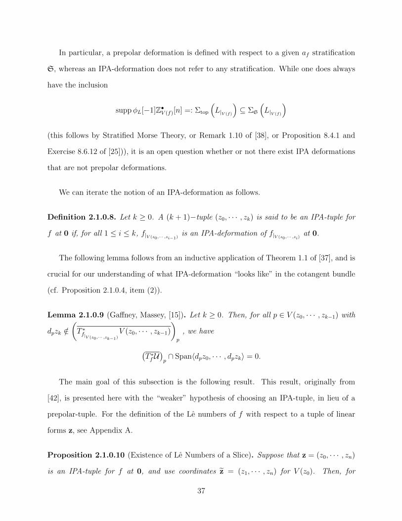
We can iterate the notion of an IPA-deformation as follows.

Definition 2.1.0.8. Let k ≥ 0. A (k + 1)−tuple (z0, · · · , zk) is said to be an IPA-tuple for

f at 0 if, for all 1 ≤ i ≤ k, f|V (z0,··· ,zi−1)is an IPA-deformation of f|V (z0,··· ,zi)

at 0.

The following lemma follows from an inductive application of Theorem 1.1 of [37], and is

crucial for our understanding of what IPA-deformation “looks like” in the cotangent bundle

(cf. Proposition 2.1.0.4, item (2)).

Lemma 2.1.0.9 (Gaffney, Massey, [15]). Let k ≥ 0. Then, for all p ∈ V (z0, · · · , zk−1) with

dpzk /∈(T ∗f|V (z0,··· ,zk−1)

V (z0, · · · , zk−1)

)p

, we have

(T ∗f U

)p∩ Span〈dpz0, · · · , dpzk〉 = 0.

The main goal of this subsection is the following result. This result, originally from

[42], is presented here with the “weaker” hypothesis of choosing an IPA-tuple, in lieu of a

prepolar-tuple. For the definition of the Le numbers of f with respect to a tuple of linear

forms z, see Appendix A.

Proposition 2.1.0.10 (Existence of Le Numbers of a Slice). Suppose that z = (z0, · · · , zn)

is an IPA-tuple for f at 0, and use coordinates z = (z1, · · · , zn) for V (z0). Then, for

37

0 ≤ i ≤ dim0 Σf , the Le numbers λif,z(0) are defined, and the following equalities hold:

λ0f|V (z0)

,z(0) =(Γ1f,z0· V (z0)

)0

+ λ1f,z(0)

λif|V (z0),z(0) = λi+1

f,z (0),

for 1 ≤ i ≤ dim0 Σf − 1, where Γ1f,z0

is the relative polar curve of f with respect to z0.

Proof. The proof follows Theorem 1.28 of [42], mutatis mutandis (changing prepolar to IPA).

Via the Chain Rule, it suffices to demonstrate that

dim0 Γi+1f,z ∩ V (f) ∩ V (z0, · · · , zi−1) ≤ 0,

since any analytic curve in Γi+1f,z ∩ V

(∂f∂zi

)∩ V (z0, · · · , zi−1) passing through 0 must be

contained in V (f), where Γi+1f,z is the (i + 1)-dimensional relative polar variety of f with

respect to z (Definition 2.1.0.2).

Suppose that we had a sequence of points p ∈ Γi+1f,z ∩ V (f)∩ V (z0, · · · , zi−1) approaching

0. As each p is contained in Γi+1f,z , for each p we can find a sequence pk → p with pk /∈ Σf

satisfying 〈dpkf〉 ⊆ Span〈dpkz0, · · · , dpkzi−1〉 for each k. But then, by construction, we have

found a nonzero element in the intersection(T ∗f U

)p∩ Span〈dpz0 · · · , dpzi−1〉, contradicting

Lemma 2.1.0.9.

2.2 Unfoldings and N•V (f)

As mentioned in the introduction of this section, we will be considering parameterized

hypersurfaces that are the total space of a family of parameterized hypersurfaces. We make

this precise with the following definition.

Definition 2.2.0.1. A parameterization π : (D× V (f0), 0 × S)→ (V (f),0) is said to be

a one-parameter unfolding with unfolding parameter t if π is of the form

π(t, z) = (t, πt(z))

38

where π0(z) := π(0, z) is a generically one-to-one parameterization of V (f, t).

We say that a parameterization π0 has an isolated instability at 0 with respect to an

unfolding π of π0 with parameter t if one has dim0 Σtopt|imπ≤ 0.

The following proposition is one of our main motivations for using IPA-deformations:

they naturally appear from one-parameter unfoldings with isolated instabilities.

Proposition 2.2.0.2. Suppose π : (D × V (f0), 0 × S) → (V (f),0) is a 1-parameter

unfolding of π0 with unfolding parameter t, such that π0 has an isolated instability at 0 with

respect to π. Then, f is an IPA-deformation of f|V (t)at 0.

Proof. By definition, π0 has an isolated instability at 0 with respect to the unfolding π with

parameter t if

dim0 Σtop

(t|V (f)

)≤ 0.

Following Definition 1.9 of [38],

Σtop

(t|V (f)

)= p ∈ V (f) | (p, dpt) ∈ SS(Z•V (f)[n])

= τ(SS(Z•V (f)[n]) ∩ im dt

),

where τ : T ∗U → U is the natural projection. This follows immediately from Proposi-

tion 2.1.0.3.

Consequently, if dim0 Σtop

(t|V (f)

)≤ 0, it follows that (0, d0t) is an isolated point in the

intersection SS(Z•V (f)[n]) ∩ im dt, and the the result follows by Proposition 2.1.0.4.

Remark 2.2.0.3. It is well-known that finitely-determined map germs π0 have isolated

instabilities with respect to a generic one-parameter unfolding ([53] pg. 241, and [14]).

Consequently, generic one-parameter unfoldings of finitely-determined maps parameterizing

hypersurfaces all give IPA-deformations.

Remark 2.2.0.4. If π is a one-parameter unfolding of a parameterization π0, then for all

t0 small, it is easy to see that there is an isomorphism N•V (f)|V (t−t0)

[−1] ∼= N•V (ft0 ), where

πt0(z) = π(t0, z).

39

Example 2.2.0.5. In the situation of Milnor’s double-point formula, π : (D×C, 0×S)→

(C3,0) parameterizes the deformation of the curve V (f0) with r irreducible components at

0 into a curve V (ft0) with only double-point singularities. Hence, dim0 V (f) = 2, and the

image multiple-point set D is purely 1-dimensional at 0.

Since π is a one-parameter unfolding with parameter t, we moreover have

N•V (f)|V (t−t0)[−1] ∼= N•V (ft0 ),

where N•V (ft0 ) is the multiple-point complex of the parameterization πt0(z). For all t0 6= 0

small, N•V (ft0 ) is supported on the set of double points of V (ft0), and at each such double-

point p we have rankH0(N•V (f0))p = |π−1(p)| − 1 = 1.

At 0 ∈ V (f0), we have π−1(0) = S, and |S| = r by assumption. Thus, rankH0(N•V (f0))0 =

r − 1.

2.3 Characteristic Polar Multiplicities

The central concept of this section, the characteristic polar multiplicities of a perverse

sheaf, were first defined and explored in [45]. These multiplicities, defined with respect to

a “nice” choice of a tuple of linear forms z = (z0, · · · , zs), are non-negative, integer-valued

functions that mimic the properties of the Le numbers associated to non-isolated hypersurface

singularities (see [42]), and the characteristic polar multiplicities of the vanishing cycles

φf [−1]Z•U [n+ 1] with respect to z coincide with the Le numbers of f with respect to z.

Definition 2.3.0.1 (Corollary 4.10 [45]). Let P• be a perverse sheaf on V (f), with dim0 supp P• =

s. Let z = (z0, · · · , zs) be a tuple of linear forms such that, for all 0 ≤ i ≤ s, we have

dim0 suppφzi−zi(p)[−1]ψzi−1−zi−1(p)[−1] · · ·ψz0−z0(p)[−1]P• ≤ 0.

Then, the i-dimensional characteristic polar multiplicity of P• with respect to z at

p ∈ V (g) is defined and given by the formula

λiP•,z(p) = rankZH0(φzi−zi(p)[−1]ψzi−1−zi−1(p)[−1] · · ·ψz0−z0(p)P

•)p.

40

Remark 2.3.0.2. In general, one can define the characteristic polar multiplicities of any

object in the bounded, derived category of constructible sheaves on V (f), but they are

slightly more cumbersome to define, and no longer need to be non-negative.

Example 2.3.0.3. Let f : U → C be an analytic function, with f(0) = 0, U an open

neighborhood of the origin in Cn+1, and dim0 Σf = s. Then, φf [−1]Z•U [n + 1] is a perverse

sheaf on V (f), with support equal to Σf∩V (f). Indeed, the containment suppφf [−1]Z•U [n+

1] ⊆ Σf∩V (f) follows from the complex analytic Implicit Function Theorem. For the reverse

containment, if p /∈ suppφf [−1]Z•U [n+ 1], then the Milnor monodromy on the nearby cycles

is the identity morphism, so that the Lefschetz number of the monodromy cannot be zero;

by A’Campo’s result [1], we therefore have p /∈ V (f) ∩ Σf .

We then have

λif,z(p) = λiφf [−1]Z•U [n+1],z(p)

for all 0 ≤ i ≤ s, and all p in an open neighborhood of 0 [45].

Remark 2.3.0.4. By Massey (Theorem 3.4 [43]), if dim0 Σf = s, then there is a chain

complex of free Abelian groups

0∂s+1−−→ Zλ

sf,z(p) ∂s−→ Zλ

s−1f,z (p) ∂s−1−−→ · · · ∂2−→ Zλ

1f,z(p) ∂1−→ Zλ

0f,z(p) ∂0−→ 0

satisfying ker ∂j/ im ∂i+1∼= Hn−j(Ff,0;Z). Since this complex is free, tensoring this complex

with Q will compute Hn−j(Ff,0;Q). Hence, we can use either Z or Q coefficients in when

characterizing the Le numbers λif,z(p) in terms of the characteristic polar multiplicities of

the vanishing cycles.

Example 2.3.0.5. If dim0 Σf = 0, any non-zero linear form z0 suffices for this construction,

since ψz0 [−1]φf [−1]Z•U [n + 1] = 0. Then, the only non-zero Le number of f is λ0f,z0

(0), and

41

we have

λ0f,z0

(0) = rankZH0(φz0 [−1]φf [−1]Z•U [n+ 1])0

= rankZH0(φf [−1]Z•U [n+ 1])0

= Milnor number of f at 0.

Example 2.3.0.6. If dim0 Σf = 1, we need z0 such that dim0 Σ(f|V (z0)

)= 0, and any

non-zero linear form suffices for z1. Then the only non-zero Le numbers of f with respect to

z = (z0, z1) are λ0f,z(0) and λ1

f,z(p) for p ∈ Σf . At 0, we have

λ1f,z(0) =

∑C⊆Σf irr.comp. at 0

µC (C · V (z0))0 ,

whereµC denotes the generic transverse Milnor number of f along C\0.

Remark 2.3.0.7. Analogous to the Le numbers λif,z(p), the characteristic polar multiplicities

of a perverse sheaf may be expressed as intersection numbers. That is, suppose we have a

perverse sheaf P• and a tuple of linear forms z such that, for all 0 ≤ i ≤ dim0 supp P•,

the characteristic polar multiplicities λiP•,z(p) are defined for all p in a neighborhood U

of 0. Then, there is a unique collection of non-negative analytic cycles ΛiP•,z called the

characteristic polar cycles of P• with respect to z satisfying, for all p ∈ U ,

λiP•,z(p) =(Λi

P•,z · V (z0 − p0, · · · , · · · , zi−1 − pi−1))p.

These cycles can also be thought of as being defined by the constructible function χ(P•)p,

so that

χ(P•)p :=∑i

(−1)iH i(P•)p =∑i

(−1)iλiP•,z(p).

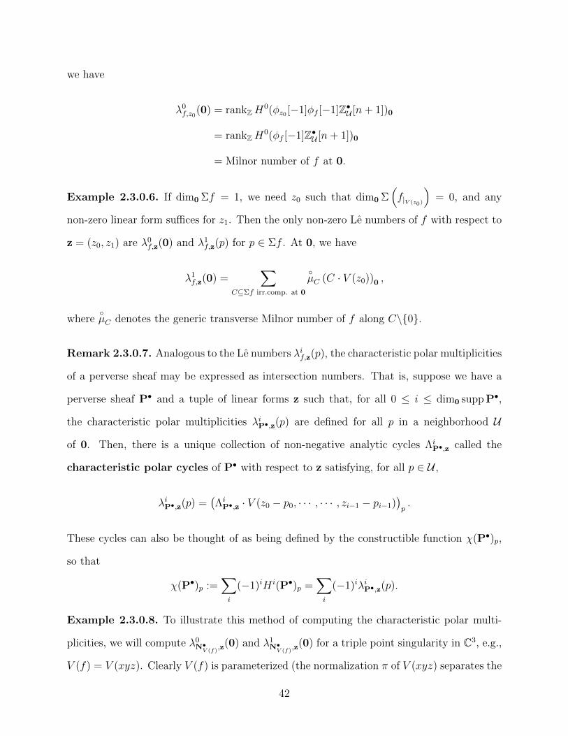
Example 2.3.0.8. To illustrate this method of computing the characteristic polar multi-

plicities, we will compute λ0N•V (f)

,z(0) and λ1N•V (f)

,z(0) for a triple point singularity in C3, e.g.,

V (f) = V (xyz). Clearly V (f) is parameterized (the normalization π of V (xyz) separates the

42

three planes into a disjoint union in three copies of C3), and so N•V (f) has stalk cohomology

concentrated in degree −1, implying

χ(N•)p = −|π−1(p)|+ 1.

Away from the origin, on the singular locus of V (xyz), χ(N•V (f))p has value −1 everywhere,

and so we can identify the 1-dimensional characteristic polar cycle of N•V (f) as the sum of

the lines of intersection of these three planes, each weighted by 1. Thus, λ1N•V (f)

,z(0) = 3.

Since χ(N•V (f))0 = −2, we find that λ0N•V (f)

,z(0) = 1, from the equality

−2 = χ(N•V (f))0 = λ0N•V (f)

,z(0)− λ1N•V (f)

,z(0) = λ0N•V (f)

,z(0)− 3.

Remark 2.3.0.9. We will need the representation of the characteristic polar multiplicities

as intersection numbers in Section 2.4 when we will use the dynamic intersection property

for proper intersections to understand λiN•V (f)

,z(0). By this, we mean the equality(Λi

P•,z · V (z0, z1, · · · , zi−1))0

=∑

p∈Bε∩ΛiP•,z∩V (z0−t)

(Λi

P•,z · V (z0 − t, z1, · · · , zi−1))p

for 0 < |t| ε 1 (see chapter 6 of [9]). Additionally, we will make use of the fact that

characteristic polar multiplicities of perverse sheaves are additive on short exact sequences

in Section 2.4. Precisely, if

0→ A• → B• → C• → 0

is a short exact sequence of perverse sheaves, and if coordinates z are generic enough so that

λiB•,z(p) is defined, then λiA•,z(p) and λiC•,z(p) are defined, and

λiB•,z(p) = λiA•,z(p) + λiC•,z(p).

(See Proposition 3.3 of [45].)

Lemma 2.3.0.10. If π is a one-parameter unfolding (with parameter t) of a parameterization

of V (f, t) with isolated instability at the origin, then the 0-dimensional characteristic polar

multiplicity of N•V (f) with respect to t is defined, and

λ0N•V (f)

,t(0) = λ0Z•V (f)

[n],t(0) =(Γ1f,t · V (t)

)0.

43

Proof. If f is an IPA-deformation of f|V (t)at 0, then dim0 suppφt[−1]Z•V (f)[n] ≤ 0, by Propo-

sition 2.1.0.4. By Definition 2.3.0.1, this is precisely what is needed to define λ0Z•V (f)

[n],t(0).

Then, by a proper base-change, we have φtπ∗ ∼= π∗φtπ, where π : V (t π) → V (f, t) is the

pullback of π via the inclusion V (f, t) → V (f). But, because π is a one-parameter unfolding,

t π is a linear form on affine space and has no critical points; hence, φtπZ•U = 0.

Consequently, it follows from the short exact sequence of perverse sheaves

0→ φt[−1]N•V (f) → φt[−1]Z•V (f)[n]→ φt[−1]π∗Z•D×X [n]→ 0

that there is an equality λ0N•V (f)

,t(0) = λ0Z•V (f)

[n],t(0), since the characteristic polar multiplicities

are additive on short exact sequences.

It is then a classical result by Le, Hamm, Teissier, and Siersma that, for sufficiently

generic t,

λ0Z•V (f)

[n],t(0) =(Γ1f,t · V (t)

)0

;

the result in the generality of IPA-deformations is found in [35]. The claim follows.

Remark 2.3.0.11. The unfolding condition is not needed for the characteristic polar mul-

tiplicities of N•V (f) to be defined, but it is needed for the vanishing λ0π∗Z•

D×V (f0)[n],t(0) = 0

which yields the equalities of Lemma 2.3.0.10.

Example 2.3.0.12. Let us compute λ0N•V (f)

,t(0) in the case where V (f) is the Whitney

umbrella, with defining function f(x, y, t) = y2− x3− tx2. Then, we can realize V (f) as the

total space of the one-parameter unfolding π(t, u) = (u2−t, u(u2−t), t) with parameter t, and

Lemma 2.3.0.10 tells us that λ0N•V (f)

,t(0) is equal to the intersection multiplicity(Γ1f,t · V (t)

)0.

A quick computation tells us that the relative polar curve Γ1f,t is equal to V (3x+ 2t, y), and

thus transversely intersects V (t) at 0. Hence,

λ0N•V (f)

,t(0) =(Γ1f,t · V (t)

)0

= 1.

The iterated IPA-condition implies the higher characteristic polar multiplicities of N•V (f)

exist as well.

44

Theorem 2.3.0.13. Suppose that (t, z) = (t, z1, · · · , zn) is an IPA-tuple for g at 0. Then,

for 0 ≤ i ≤ n − 1, the characteristic polar multiplicities λiN•V (f)

,(t,z)(0) with respect to (t, z)

are defined, and the following equalities hold:

λ0N•V (f0)

,z(0) = λ1N•V (f)

,(t,z)(0)− λ0N•V (f)

,(t,z)(0),

and, for 1 ≤ i ≤ n− 2,

λiN•V (f0)

,z(0) = λi+1N•V (f)

,(t,z)(0).

Proof. That λ0N•V (f)

,(t,z)(0) is defined is precisely the inequality dim0 suppφt[−1]N•V (f) ≤ 0

concluded in Lemma 2.3.0.10 from the short exact sequence

0→ φt[−1]N•V (f) → φt[−1]Z•V (f)[n]→ φt[−1]π∗Z•D×V (f0)[n]→ 0.

By Proposition 3.2 of [45], it remains to show that λiN•V (f)

,(t,z)(0) is defined for 1 ≤ i ≤ n− 1,

i.e., we need to show that

dim0 suppφzi−1[−1]ψzi−2

[−1] · · ·ψz1 [−1]ψt[−1]N•V (f) ≤ 0.

From the short exact sequence of perverse sheaves

0→ N•V (f) → Z•V (f)[n]→ π∗Z•D×V (f0)[n]→ 0,

it follows that λiN•V (f)

,(t,z)(0) is defined if λiZ•V (f)

[n],(t,z)(0) is defined, by the triangle inequality

for supports of perverse sheaves.

Since (t, z) is an IPA-tuple for f at 0, Proposition 2.1.0.4 gives, for 1 ≤ i ≤ n− 1,

dim0 suppφzi [−1]Z•V (f,t,z1,··· ,zi−1)[n− i] ≤ 0.

Thus, away from 0, each of the comparison morphisms

Z•V (f,t,z1,··· ,zi−1,zi)[n− i− 1]

∼→ ψzi [−1]Z•V (f,t,z1,··· ,zi−1)[n− i]

is an isomorphism for 1 ≤ i ≤ n− 1. Consequently,

dim0 suppφzi [−1]Z•V (f,t,z1,··· ,zi−1)[n− i] ≤ 0

45

implies

dim0 suppφzi−1[−1]ψzi−2

[−1] · · ·ψz1 [−1]ψt[−1]Z•V (f)[n] ≤ 0,

and the claim follows.

Remark 2.3.0.14. In the wake of a recent paper [39] by David Massey, we can obtain

a much simpler proof of the above result; one has the identification N•V (f)∼= kerid−Tf

for hypersurfaces, where Tf is the Milnor monodromy automorphism on the vanishing cy-

cles φf [−1]Z•U [n + 1]. Consequently, N•V (f) is a perverse subobject of the vanishing cycles

φf [−1]Z•U [n + 1], and we obtain Theorem 2.3.0.13 by either the triangle inequality for mi-

crosupports, or the fact that characteristic polar multiplicities are additive on short exact

sequences [45] from the fact that supp N•V (f) ⊆ suppφf [−1]Z•U [n+ 1] = Σf .

2.4 Milnor’s Result and Beyond

We wish to express the Le numbers of f0 entirely in terms of data from the Le numbers

of ft0 and the characteristic polar multiplicities of both N•V (f0) and N•V (ft0 ), for t0 small and

nonzero. The starting point is Proposition 2.1.0.10:

λ0f0,z

(0) =(Γ1f,t · V (t)

)0

+ λ1f,(t,z)(0)

λift0 ,z(0) = λi+1f,(t,z)(0),

where (t, z) = (t, z1, · · · , zn) is an IPA-tuple for f at 0. From Lemma 2.3.0.10, we have(Γ1f,t · V (t)

)0

= λ0N•V (f)

,(t,z)(0); we now have all our relevant data in terms of Le numbers and

characteristic polar multiplicities of N•V (f). The goal is then to decompose this data into

numerical invariants which refer only to the t = 0 and t 6= 0 slices of V (f).

So, in order to realize this goal, the next step is to decompose λ0N•V (f)

,(t,z)(0) and λif,(t,z)(0)

for i ≥ 1.

46

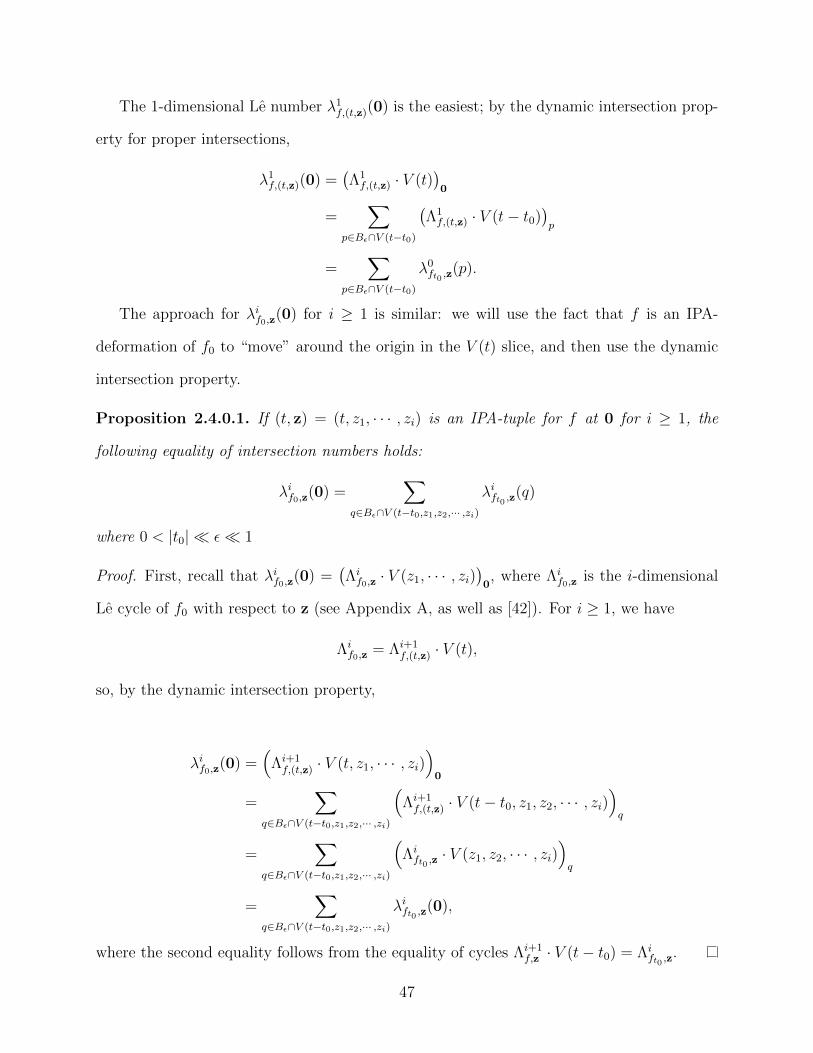
The 1-dimensional Le number λ1f,(t,z)(0) is the easiest; by the dynamic intersection prop-

erty for proper intersections,

λ1f,(t,z)(0) =

(Λ1f,(t,z) · V (t)

)0

=∑

p∈Bε∩V (t−t0)

(Λ1f,(t,z) · V (t− t0)

)p

=∑

p∈Bε∩V (t−t0)

λ0ft0 ,z

(p).

The approach for λif0,z(0) for i ≥ 1 is similar: we will use the fact that f is an IPA-

deformation of f0 to “move” around the origin in the V (t) slice, and then use the dynamic

intersection property.

Proposition 2.4.0.1. If (t, z) = (t, z1, · · · , zi) is an IPA-tuple for f at 0 for i ≥ 1, the

following equality of intersection numbers holds:

λif0,z(0) =

∑q∈Bε∩V (t−t0,z1,z2,··· ,zi)

λift0 ,z(q)

where 0 < |t0| ε 1

Proof. First, recall that λif0,z(0) =

(Λif0,z· V (z1, · · · , zi)

)0, where Λi

f0,zis the i-dimensional

Le cycle of f0 with respect to z (see Appendix A, as well as [42]). For i ≥ 1, we have

Λif0,z

= Λi+1f,(t,z) · V (t),

so, by the dynamic intersection property,

λif0,z(0) =

(Λi+1f,(t,z) · V (t, z1, · · · , zi)

)0

=∑

q∈Bε∩V (t−t0,z1,z2,··· ,zi)

(Λi+1f,(t,z) · V (t− t0, z1, z2, · · · , zi)

)q

=∑

q∈Bε∩V (t−t0,z1,z2,··· ,zi)

(Λift0 ,z· V (z1, z2, · · · , zi)

)q

=∑

q∈Bε∩V (t−t0,z1,z2,··· ,zi)

λift0 ,z(0),

where the second equality follows from the equality of cycles Λi+1f,z · V (t− t0) = Λi

ft0 ,z.

47

We can now state and prove our main result.

Theorem 2.4.0.2. Suppose that π : (D × V (f0), 0 × S) → (V (f),0) is a one-parameter

unfolding with an isolated instability of a parameterized hypersurface imπ0 = V (f0). Suppose

further that z = (z1, · · · , zn) is chosen such that z is an IPA-tuple for f0 = f|V (t)at 0.

Then, the following formulas hold for the Le numbers of f0 with respect to z at 0: for

0 < |t0| ε 1,

λ0f0,z

(0) = −λ0N•V (f0)

,z(0) +∑

p∈Bε∩V (t−t0)

(λ0ft0 ,z

(p) + λ0N•V (ft0

),z(p)

),

and, for 1 ≤ i ≤ n− 2,

λif0,z(0) =

∑q∈Bε∩V (t−t0,z1,z2,··· ,zi)

λift0 ,z(q).

In particular, the following relationship holds for 0 ≤ i ≤ n− 2:

λif0,z(0) + λiN•

V (f0),z(0) =

∑p∈Bε∩V (t−t0,z1,z2,··· ,zi)

(λift0 ,z(p) + λiN•

V (ft0),z(p)

)Proof. By Proposition 2.1.0.10 and Proposition 2.4.0.1, it suffices to prove

λ0N•V (f)

,(t,z)(0) = −λ0N•V (f0)

,z(0) +∑

p∈Bε∩V (t−t0)

λ0N•V (ft0

),z(p). (2.4)

Since (t, z) is an IPA-tuple for f at 0, Theorem 2.3.0.13 yields

λ0N•V (f0)

,z(0) = λ1N•V (f)

,(t,z)(0)− λ0N•V (f)

,(t,z)(0),

where N•V (f0)∼= N•V (f)|V (t)

[−1] (cf. Remark 2.2.0.4).

The main claim then follows by the dynamic intersection property for proper intersections

applied to Λ1N•V (f)

,(t,z) (see Remark 2.3.0.9):

λ1N•V (f)

,(t,z)(0) =(

Λ1N•V (f)

,(t,z) · V (t))0

=∑

p∈Bε∩V (t−t0)

(Λ1

N•V (f)

,(t,z) · V (t− t0))p

=∑

p∈Bε∩V (t−t0)

λ0N•V (ft0

),z(p),

48

for 0 < |t0| ε 1.

Finally, we examine the relationship

λif0,z(0) + λiN•

V (f0),z(0) =

∑p∈Bε∩V (t−t0,z1,z2,··· ,zi)

(λift0 ,z(p) + λiN•

V (ft0),z(p)

).

For i = 0, this follows by a trivial rearrangement of the terms in our expression for λ0f0,z

(0).

For i ≥ 1, this is just Proposition 2.4.0.1 combined with Theorem 2.3.0.13 and the dynamic

intersection property on λiN•V (f)

,(t,z)(0), as in Proposition 2.4.0.1 for λif,(t,z)(0).

Remark 2.4.0.3. The relationship

λif0,z(0) + λiN•

V (f0),z(0) =

∑p∈Bε∩V (t−t0,z1,z2,··· ,zi)

(λift0 ,z(p) + λiN•

V (ft0),z(p)

)

suggests a sort of “conserved quantity” between the sum of the Le numbers of ft and the

characteristic polar multiplicities of N•V (ft)in one parameter deformations of parameterized

hypersurfaces. It is a very interesting question to see how this relates to results in Chapter 3

and the isomorphism N•V (f)∼= kerid−Tf (see Section 1.2 and Section 3.4).

Example 2.4.0.4. We wish to examine Theorem 2.4.0.2 in the context of Milnor’s double

point formula, where π : (D×C, 0×S)→ (C3,0) parameterizes a deformation of the curve

V (f0) into a curve V (ft0) with only double-point singularities. In this case, dim0 Σf0 = 0,

so the only non-zero Le number of f0 is λ0f0,z

(0), where z is any non-zero linear form on C2,

and λ0f0,z

(0) = µ0(f0).

It is then an easy exercise to see that λ0N•V (ft0

),z(p) = m(p) = |π−1(p)| − 1 for t0 small

(and possibly zero) and p ∈ D.

All together, this gives, by Theorem 2.4.0.2

µ0(f0) = −(r − 1) +∑

p∈Bε∩V (t−t0)

(µp(ft0) + |π−1(p)| − 1

)= 2δ − r + 1,

49

as there are δ double-points in the deformed curve V (ft0). We have thus recovered Milnor’s

original double-point formula for the Milnor number of a plane curve singularity. We picture

this computation below.

Remark 2.4.0.5. In Lemma 2.2 of [56], David Mond also obtains the result that, for a

stabilization of a plane curve singularity V (f0), one has

µ0

(t|V (f)

)= δ − r + 1,

where µ0

(t|V (f)

)is called the image Milnor number of the stabilization. It is an inter-

esting question in general how one can relate the theory of map germs from Cn to Cn+1

of finite A-codimension (in Mather’s nice dimensions (n < 15) and beyond) to our result

Theorem 2.4.0.2.

Remark 2.4.0.6. Gaffney also generalizes the result µ0(t|V (f)) = δ− r+ 1 in [13], although

to the very different setting of maps G : (Cn, S) → (C2n,0). In Theorem 3.2 and Corollary

3.3 of [13], this formula is derived in terms of the Segre number of dimension 0 of an ideal

associated to the image multiple-point set D and the number of Whitney umbrellas of the

composition of the map G with a generic projection to C2n−1.

In analogy to plane curve singularities deforming into node singularities, it is well-known

(see, e.g., [57]), that for stabilizations of finitely determined maps π0 : (C2, S)→ (C3,0), the

50

image surface im π0 = V (f0) splits into Cross Caps (i.e., Whitney Umbrellas), Triple Points,

and A1-singularities (i.e., nodes, which appear off the hypersurface on the relative polar

curve). Unfortunately, detecting these invariants using characteristic polar multiplicities

and Theorem 2.4.0.2 will have an unavoidable problem: we will also see points that belong

to the absolute polar curve Γ1z(Σf), which lie in the smooth part of Σf near 0, and are

artifacts of our choice of linear forms z in calculating the characteristic polar multiplicities.

For z = (t, z) a generic pair of linear forms on C4, the absolute polar curve of Σf at 0 is

Γ1z(Σf) = Σ

((t, z)|Σf

)− Σ(Σf)

(see [31], [70], but we instead index by dimension instead of codimension). Consequently,

if p ∈ Γ1z(Σf)\0, we see that λ0

N•V (ft0

),z(p) 6= 0 even if the stalk cohomology of N•V (ft0 ) is

locally constant near p. We thus obtain the following result:

Theorem 2.4.0.7. Suppose π : (D×C2, 0×S)→ (C4,0) is a one-parameter unfolding of

a finitely-determined map germ π0 : (C2, S)→ (C3,0) parameterizing a surface V (f0) ⊆ C3.

Then,

λ0N•V (f0)

,z(0) = T + C − δ + P

where T,C, δ, and P denote the number of triple points, cross caps, A1-singularities appear-

ing in a stable deformation of V (f0), respectively, and if V (f) = im π, P denotes the number

of intersection points of the absolute polar curve Γ1(t,z)(Σf) with a generic hyperplane V (z)

on C4 for which (t, z) is an IPA-tuple for f at 0.

Proof. This follows directly from Theorem 2.3.0.13, Remark 2.2.0.3, Lemma 2.3.0.10, and

recalling that λ0N•V (ft0

),z(0) = 1 for both Whitney umbrellas and triple point singularities in

C3 (see Example 2.3.0.12 and Example 2.3.0.8).

In fact, we can explicitly identify the Euler characteristic λ0N•V (f0)

,z(0)−λ1N•V (f0)

,z(0) using

Theorem 2.4.0.7.

51

Corollary 2.4.0.8. Let π0, π, T,C, δ, and P be as in Theorem 2.4.0.7. Then, the following

equalities hold:

λ0N•V (f0)

,z(0)− λ1N•V (f0)

,z(0) = χ(N•V (f0))0 = −|π−10 (0)|+ 1 = C − T − δ − χ(Ft|Σf ,0),

where Ft|Σf ,0 denotes the complex link of Σf at 0.

Remark 2.4.0.9. Before we give the proof of Corollary 2.4.0.8 using derived category tech-

niques, we will give a down-to-earth topological argument. The key idea in our proof is

that one can compute the term P using constant Z coefficients instead of N•V (f), since N•V (f)

generically has stalk cohomology Z along Σf for hypersurfaces V (f) that are the image of

finitely-determined map germs.

Proof. (topological argument) We compute the Euler characteristic of the pair χ(Ft|Σf ,0, Fz|Σf0 ,0).

This pair of subspaces makes sense, using the fact that f is an IPA-deformation of f0, and

the complex link Fz|Σf0 ,0of Σf0 is a finite set of points, and their multiplicity is unchanged

as one moves in the t direction away from the origin, pictured below:

Thus, we can identify Fz|Σf0 ,0= Bε ∩ Σf ∩ V (t, z − b) with Bε ∩ Σf ∩ V (t − a, z − b) for

0 < |a| |b| ε 1. Consequently, we can identify

χ(Ft|Σf ,0, Fz|Σf0 ,0) = χ(φz[−1]Z•Ft|Σf ,0

[1])0 =∑p

λ0Z•Σft0

[1],z(p).

52

As the value of z grows from 0 to b, we pick up cohomological contributions (in the form of

a non-zero multiplicity λ0Z•Σft0

[1],z(p)) as we pass through points of the curves of triple points,

cross caps, and the absolute polar curve with respect to (t, z), pictured below:

At triple points, λ0Z•Σft0

[1],z(p) = 2, and at cross caps λ0Z•Σft0

[1],z(p) = 0. We count the contri-

bution from the absolute polar curve as P =(

Γ1(t,z)(Σf) · V (z)

)0. Thus,

2T + P = χ(Ft|Σf ,0, Fz|Σf0 ,0) = χ(Ft|Σf ,0)− χ(Fz|Σf0 ,0

)

= χ(Ft|Σf ,0)− λ1N•V (f0)

,z(0).

Solving for P and plugging the resulting expression into Theorem 2.4.0.7 gives the result.

Proof. (perverse sheaves argument) We wish to better understand the contribution of the

term P coming from the absolute polar curve of Σf appearing in Theorem 2.4.0.7. First,

we note that these terms come from the 0-dimensional characteristic polar multiplicities

λ0N•V (ft0

),z(p) in the expansion of λ1

N•V (f)

,(t,z)(0), where p is a smooth point of Σf in the V (t−t0)

slice. Since the transverse singularity type of the image of a finitely-determined map is always

that of a Morse function, the stalk cohomology of N•V (f) is Z at all smooth points of Σf .

Consequently, we can calculate P using the constant sheaf Z•Σf [2] in place of N•V (f).

53

However, Z•Σf [2] is not necessarily a perverse sheaf. To deal with this, note that, for all

t0 6= 0, the restriction(Z•Σf [2]

)|V (t−t0)

∼= Z•Σft0 [1] is a perverse sheaf (the shifted constant

sheaf on a curve is always perverse), and therefore ψt[−1]Z•Σf [2] is perverse.

We then examine Euler characteristics at the origin of the distinguished triangle

(ψt[−1]Z•Σf [2]

)|V (z)

[−1]→ ψz[−1]ψt[−1]Z•Σf [2]→ φz[−1]ψt[−1]Z•Σf [2]+1−→, (2.5)

where ψz[−1]ψt[−1]Z•Σf [2] and φz[−1]ψt[−1]Z•Σf [2] are perverse sheaves for which 0 is an

isolated point in their support. By Definition 2.3.0.1,

χ(φz[−1]ψt[−1]Z•Σf [2])0 = rankH0(φz[−1]ψt[−1]Z•Σf [2])0 = λ1Z•Σf [2],(t,z)(0).

To calculate χ(ψz[−1]ψt[−1]Z•Σf [2])0, note that dim0 suppφt[−1]Z•Σf [2] ≤ 0 (since f is

an IPA-deformation of f|V (t)at 0) implies ψz[−1]φt[−1]Z•Σf [2] = 0, and so

ψz[−1]Z•Σf0[1]

∼−→ ψz[−1]ψt[−1]Z•Σf [2].

Thus, χ(ψz[−1]ψt[−1]Z•Σf [2])0 = χ(ψz[−1]Z•Σf0[1])0 = λ1

Z•Σf0 [1],z(0). It is easy to see that

λ1Z•Σf0 [1],z(0) = λ1

N•V (f0)

,z(0), since the transverse singularity type of Σf0 is that of a Morse

function.

Finally, we see that χ((ψt[−1]Z•Σf [2]

)|V (z)

[−1])0 = χ(Ft|Σf ,0), and we obtain the following

formula from taking the Euler characteristic of (2.5):

χ(Ft|Σf ,0)− λ1N•V (f0)

,z(0) + λ1Z•Σf [2],(t,z)(0) = 0. (2.6)

Using the dynamic intersection property,

λ1Z•Σf [2],(t,z)(0) =

∑p∈Bε∩V (t−t0)

λ0Z•Σft0

[1],z(p) = 2T + P,

since λ0Z•Σft0

[1],z(p) = 2 when p is a triple point singularity, and λ0Z•Σft0

[1],z(p) = 0 when p is a

cross-cap singularity. The remaining terms, as in Theorem 2.4.0.7, come from the absolute

polar curve of Σf with respect to V (z). Consequently, we can solve for P using (2.6)

P = λ1N•V (f0)

,z(0)− χ(Ft|Σf ,0)− 2T.

54

Plugging this expression for P into Theorem 2.4.0.7 tells us

λ0N•V (f0)

,z(0) = T + C − δ + P

= T + C − δ + λ1N•V (f0)

,z(0)− χ(Ft|Σf ,0)− 2T

and so

χ(N•V (f0))0 = λ0N•V (f0)

,z(0)− λ1N•V (f0)

,z(0) = C − T − δ − χ(Ft|Σf ,0).

Finally, the Corollary follows from the fact that N•V (f0) has stalk cohomology concentrated

in degree −1 (by Theorem 1.1.1.4 and Remark 2.3.0.7)

Remark 2.4.0.10. If V (f0) is itself a Q-homology manifold, then N•V (f0) = 0. In this case,

Theorem 2.4.0.7 tells us that, in a stabilization V (f) of V (f0), we have

χ(Ft|Σf ,0) = C − T − δ.

Remark 2.4.0.11. In the case of finitely-determined maps F : (C2,0) → (C3,0) of the

form F (t, z2, F3(t, z)), imF = V (f) defines a surface whose singular locus Σf is an isolated

complete intersection singularity (ICIS) by results of Mond and Pellikaan (e.g., Prop. 2.2.4 of

[58]). In this case, the results of [12] apply, and we can recover Gaffney’s formula (Proposition

2.4) for the 0-dimensional Le number of f at 0

λ0f,z(0) = δ + 2C + e(JM(Σf)).

where δ (resp., C) is the number of A1-singularities (resp., cross caps) appearing in a stabi-

lization of F , and e(JM(Σf)) is the Buchbaum-Rim multiplicity of the Jacobian Module of

Σf = D.

It is a very interesting question to see what formulas might arise from Theorem 2.4.0.2

when one works outside of Mather’s nice dimensions; for n ≥ 15, one can no longer approx-

imate a finitely determined map with stable maps, but the relationship in Theorem 2.4.0.2

still holds.

55

Chapter 3

Some Hodge Theoretic Aspects of

Parameterized Spaces

This chapter arose from an innocuous question posed to us by a referee of [21]: when

is N•X a semi-simple perverse sheaf, so that Q•X [n] is an extension of semi-simple

perverse sheaves?

We were able to provide a somewhat “unsatisfying” partial answer (below) to this ques-

tion in Remark 2.5 of [21] in response to this referee; later, we provided a complete answer

that eventually became [22]. It is this complete answer, and the details involved, that we

will present in this chapter.

When X is a parameterized space, both I•X and N•X are, in fact, just sheaves (up to a

shift); moreover, the short exact sequence of perverse sheaves

0→ N•X → Q•X [n]→ I•X → 0

can be rewritten as a short exact sequence of (constructible) sheaves

0→ QX → H−n(I•X)→ H−n+1(N•X)→ 0.

One can then find a Whitney stratification S of X for which the sets Xk (see Formula 1.6)

are locally finite unions of strata for all k. Then, for each stratum S ⊂ Xk, the monodromy

56

of the local system N•X |S is determined by the monodromy of the set π−1(p) for p ∈ S; since

this is a finite set with k elements, it follows immediately that N•X |S is semi-simple as a

local system on S (since the monodromy action is semi-simple).

Since N•X |S is semi-simple as a local system for any stratum S ⊂ Xk, is N•X semi-simple

as a perverse sheaf? If one has a Whitney stratification of X for which the sets Xk are finite

unions of strata, and for which the subset D = supp N•X is a union of closed strata, then the

above argument demonstrates (together with Section 2.4 of [67]) that N•X is semi-simple as

a perverse sheaf. In general, however, this fails to be the case (see Subsection 1.1.2).

More generally, when Q•X [n] is a perverse sheaf, one may use the general machinery of

mixed Hodge modules developed by M. Saito (see [66], page 325, formula (4.5.9)) to obtain

an isomorphism of perverse sheaves

GrWn Q•X [n]∼→ I•X . (3.1)

underlying the corresponding isomorphism of mixed Hodge modules. Since dim0X = n, the

weight filtration on Q•X [n] terminates after degree n, so that WnQ•X [n] ∼= Q•X [n]. Conse-

quently, the above isomorphism yields a short exact sequence

0→ Wn−1Q•X [n]→ Q•X [n]→ I•X → 0

of perverse sheaves on X, implying N•X∼= Wn−1Q•X [n]. From this identification, it fol-

lows that N•X is semi-simple as a perverse sheaf provided that the induced weight filtra-

tion WiQ•X [n] of Wn−1Q•X [n] ∼= N•X for i < n is concentrated in one degree k < n, i.e.,

WiQ•X [n] = 0 for i < k and WiQ•X [n] ∼= WkQ•X [n] for k < i < n. Then, N•X∼= GrWk Q•X [n]

underlies a pure polarizable Hodge module, which is therefore by construction a semi-simple

perverse sheaf. Identifying when this happens is quite involved and will be the focus of this

chapter, with a complete answer proved in Theorem 3.2.0.6 and Corollary 3.2.0.7.

57

3.1 Introduction

Let U be an open neighborhood of the origin in CN , and let X ⊆ U be a purely n

dimensional reduced complex analytic space on which Q•X [n] is perverse.

By shrinking U if necessary, the perverse sheafQ•X [n] underlies a graded-polarizable mixed

Hodge module (Prop 2.19, Prop 2.20, [66]) of weight ≤ n. Moreover, by Saito’s theory of

(graded polarizable) mixed Hodge modules in the local complex analytic context, the perverse

cohomology objects of the usual sheaf functors naturally lift to cohomology functors in the

context of (graded polarizable) mixed Hodge modules (but not on their derived category level

as in the algebraic context as in Section 4 of [66]). As above in Formula 3.1, the quotient

morphism Q•X [n]→ I•X induces an isomorphism

GrWn Q•X [n] ∼= I•X ;

consequently, the fundamental short exact sequence (1.1) identifies the comparison complex

N•X with Wn−1Q•X [n]. In this chapter, we explicitly identify the graded piece GrWn−1 N•X =

GrWn−1Q•X [n] in the case where X is a parameterized space, and give concrete computations

of W0Q•X [n] in the case where X = V (f) is a parameterized surface in C3.

Let ΣX denote the singular locus of X, and let i : ΣX → X. We can then find a

smooth, Zariski open dense subset W ⊆ ΣX over which the normalization map restricts to

a covering projection π : π−1(W)→W ⊆ ΣX (see Section 6.2, [16]). Let l :W → ΣX and

m : ΣX\W → ΣX denote the respective open and closed inclusion maps. Let m := i m,

l := i l. Note that dim0 ΣX\W ≤ n− 2, as it is the complement of a Zariski open set (we

will need this later in Proposition 3.2.0.2).

Example 3.1.0.1. Consider the Whitney umbrella V (f) ⊆ C3 with f(x, y, t) = y2−x3−tx2.

Then, the normalization of V (f) is smooth, and given by the map π(t, u) = (u2 − t, u(u2 −

t), t).

58

The critical locus of f is Σf = V (x, y), and it is easy to see that over Σf\0, π is a

2-to-1 covering map; thus, we set W = Σf\0.

Example 3.1.0.2. Suppose V (f) ⊆ C3 is a parameterized surface. Then, it is easy to see

that W = Σf\0; this follows from the fact that I•V (f)|Σfis is constructible with respect

to the Whitney stratification Σf\0, 0 of Σf , along with the description of the stalk

cohomology of I•V (f) given by the isomorphism I•V (f)∼= π∗Q•

V (f)[2], where π : V (f) → V (f)

is the normalization of V (f).

We will examine this setting in more detail in Section 3.3

Our main result of this chapter is the following.

Theorem 3.1.0.3 (Theorem 3.2.0.6). Suppose X is a parameterized space. Then, there

is an isomorphism GrWn−1 i∗N•X

∼= I•ΣX(l∗N•X), so that the short exact sequence of perverse

sheaves on X

0→ m∗pH0(m!i∗N•X)→ i∗N•X → I•ΣX(l∗N•X)→ 0

identifies Wn−2i∗N•X

∼= m∗pH0(m!i∗N•X). Here, I•ΣX(l∗N•X) denotes the intermediate ex-

tension of the perverse sheaf l∗N•X to all of ΣX, and pH0(−) denotes the 0-th perverse

cohomology functor.

Since the map i : ΣX → X is a closed inclusion, it preserves weights. Moreover, the

support of N•X is contained in the singular locus ΣX, and so i∗i∗N•X

∼= N•X . Consequently,

we have the following.

Corollary 3.1.0.4 (Corollary 3.2.0.7, Theorem 3.2.0.8). Suppose X is a parameterized space.

Then, there are isomorphisms

GrWn−1Q•X [n] ∼= GrWn−1 i∗N•X

∼= i∗I•ΣX(l∗N•X),

and

Wn−2Q•X [n] ∼= Wn−2i∗N•X

∼= m∗pH0(m!i∗N•X) ∼= m′∗ kerφg[−1]i∗N•X

var−→ ψg[−1]i∗N•X,

59

where g is any complex analytic function on ΣX such that V (g) contains ΣX\W, but does

not contain any irreducible component of ΣX, and m′ : V (g) → ΣX is the closed inclusion.

In the case where X = V (f) is a parameterized surface in C3, we explicitly compute

W0Q•V (f)[2]; the vanishing of this perverse sheaf places strong constraints on the topology of

the singular set Σf of V (f); we will see this later in Theorem 3.3.0.1.

3.2 General Case for Parameterized Spaces

In this section, we first prove a general result, Lemma 3.2.0.1, about perverse sheaves

that will allow us to construct the short exact sequence mentioned in Theorem 3.2.0.6, and

that N•X satisfies the hypotheses of this lemma provided that X is parameterized. Then,

we examine the weight filtration on I•ΣX(l∗N•X) and show that it underlies a polarizable

Hodge module of weight n− 1 in Proposition 3.2.0.5. With all this, we can state and prove

Theorem 3.2.0.6 and Corollary 3.2.0.7.

Recall the category of perverse sheaves Perv(X) is the Abelian subcategory of the bounded

derived category of sheaves of Q-vector spaces with C-constructible cohomology Dbc(X) given

by the heart of the perverse t-structure, Perv(X) = pD≤0(X) ∩ pD≥0(X). Here,

• P• ∈ pD≤0(X) if P• satisfies the support condition: for all k ∈ Z,

dimC suppHk(P•) ≤ −k.

• P• ∈ pD≥0(X) if DP• satisfies the support condition, where D denotes the Verdier

duality functor. This is known as the cosupport condition.

.

The following lemma is due to the author and David Massey.

60

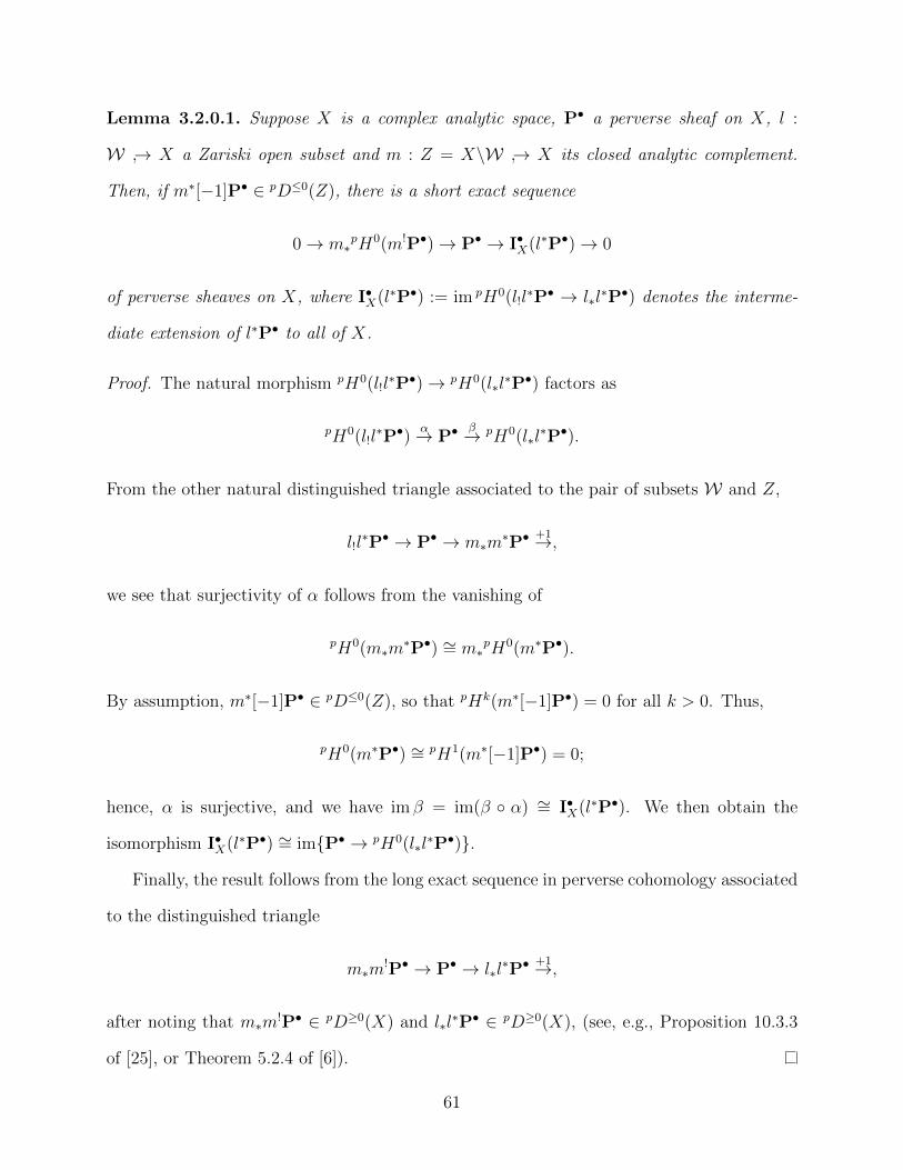
Lemma 3.2.0.1. Suppose X is a complex analytic space, P• a perverse sheaf on X, l :

W → X a Zariski open subset and m : Z = X\W → X its closed analytic complement.

Then, if m∗[−1]P• ∈ pD≤0(Z), there is a short exact sequence

0→ m∗pH0(m!P•)→ P• → I•X(l∗P•)→ 0

of perverse sheaves on X, where I•X(l∗P•) := im pH0(l!l∗P• → l∗l

∗P•) denotes the interme-

diate extension of l∗P• to all of X.

Proof. The natural morphism pH0(l!l∗P•)→ pH0(l∗l

∗P•) factors as

pH0(l!l∗P•)

α→ P•β→ pH0(l∗l

∗P•).

From the other natural distinguished triangle associated to the pair of subsets W and Z,

l!l∗P• → P• → m∗m

∗P•+1→,

we see that surjectivity of α follows from the vanishing of

pH0(m∗m∗P•) ∼= m∗

pH0(m∗P•).

By assumption, m∗[−1]P• ∈ pD≤0(Z), so that pHk(m∗[−1]P•) = 0 for all k > 0. Thus,

pH0(m∗P•) ∼= pH1(m∗[−1]P•) = 0;

hence, α is surjective, and we have im β = im(β α) ∼= I•X(l∗P•). We then obtain the

isomorphism I•X(l∗P•) ∼= imP• → pH0(l∗l∗P•).

Finally, the result follows from the long exact sequence in perverse cohomology associated

to the distinguished triangle

m∗m!P• → P• → l∗l

∗P•+1→,

after noting that m∗m!P• ∈ pD≥0(X) and l∗l

∗P• ∈ pD≥0(X), (see, e.g., Proposition 10.3.3

of [25], or Theorem 5.2.4 of [6]).

61

From the introduction, let ΣX denote the singular locus of X, and let i : ΣX → X.

We can then find a smooth, dense Zariski open dense subset W ⊆ ΣX over which the

normalization map restricts to a covering projection π : π−1(W) → W ⊆ ΣX (see Section

6.2, [16]). Let l : W → ΣX and m : ΣX\W → ΣX denote the respective open and closed

inclusion maps. Let m := i m, l := i l. Note that dim0 ΣX\W ≤ n − 2, as it is the

complement of a Zariski open set.

Proposition 3.2.0.2. If X is a parameterized space, then m∗[−1]N•X ∈ pD≤0(ΣX\W).

Proof. We wish to show that for all k ∈ Z,

dimC suppHk(m∗[−1]N•X) ≤ −k.

However, since X is parameterized, suppHk(m∗[−1]N•X) is non-empty only for k−1 = −n+1

by Theorem 1.1.1.4, i.e., when k = −n + 2. In this degree, the support is equal to ΣX\W .

Since this set is the complement of a Zariski open dense subset of ΣX,

dimC suppH−n+2(m∗N•X) ≤ n− 2,

as desired.

Remark 3.2.0.3. For surfacesX = V (f) with curve singularities, m∗[−1]N•V (f) ∈ pD≤0(Σf\W)

if and only if V (f) is a parameterized space. To see this, first note by Example 3.1.0.2 that

m is the inclusion of a point, and thus pD≤0(Σf\W) = D≤0(Σf\W), i.e., the perverse t-

structure on a point is the standard t-structure. Hence, m∗[−1]N•V (f) ∈ pD≤0(Σf\W) if and

only if Hk(N•V (f))0 = 0 for k > −1. For surfaces with curve singularities, this implies that the

stalk cohomology of N•V (f) at the origin is concentrated in degree −1. By Theorem 1.1.1.4,

this is equivalent to V (f) being a parameterized space.

In general, m∗[−1]N•X ∈ pD≤0(ΣX\W) places strict constraints on the possible coho-

mology groups of the real link of X, denoted KX,p, at different points p ∈ ΣX, i.e., the

intersection of X with a sphere of sufficiently small radius at p.

62

Remark 3.2.0.4. Generically along an irreducible component C of ΣX, N•X is isomorphic

to a local system l∗(N•X |C ) in degree −n+ 1, and in that degree, we have

H−n+1(N•X)p ∼= IH0(Bε(p) ∩X;Q)

where IHk

denotes reduced intersection cohomology (with topological indexing, as in [17]).

This description follows immediately from the fundamental short exact sequence (1.1). Since

I•X∼= π∗Q•X [n], this reduced intersection cohomology is actually just

IH0(Bε(p) ∩X;Q) ∼= H0(KX,π−1(p);Q),

where

KX,π−1(p) =⋃

q∈π−1(p)

KX,q.

Since X is normal (and thus locally irreducible) it is clear that one has H0(KX,q;Q) ∼= Q

for all q ∈ X. After noting that H−n(I•X)p = IH0(KX,p) (that is, intersection cohomology

of KX,p with topological indexing), H−n(I•X)p has a pure Hodge structure of weight 0 (see,

e.g., A. Durfee and M. Saito [7]).

Proposition 3.2.0.5. Let C be an irreducible component of ΣX at 0. Then, l∗(N•X |C )

underlies a polarizable variation of Hodge structure of weight 0.

Consequently, I•ΣX(l∗N•X) underlies a polarizable Hodge module of weight n− 1 on ΣX.

Proof. Since l∗N•X underlies a mixed Hodge module whose underlying perverse sheaf is a local

system (up to a shift) on the complex manifold U , this local system underlies an admissable

graded polarizable variation of mixed Hodge structures on U by Theorem 3.27 of [66].

To show that this mixed Hodge structure is pure of weight zero, we can check on stalks

at points p ∈ U . Let ip : p → U ; then, the stalk cohomology Hk(−)p agrees with

perverse cohomology pHk(i∗p). So, applying Hk(i∗p) on the level of mixed Hodge modules to

the fundamental short exact sequence (1.1), we get (by Proposition 2.19, Proposition 2.20,

63

and Theorem 3.9 of [66]) a short exact sequence in the category of graded polarizable mixed

Hodge structures, whose underlying sequence of vector spaces is

0→ Qp → H−n(I•X)p → H−n+1(N•X)p → 0. (3.2)

However, π : X → X is a finite map, and therefore exact for the perverse t-structure (and

mixed Hodge modules), with

H−n(I•X)p ∼= H−n(π∗Q•X [n])p ∼=⊕

y∈π−1(p)

Qy.

Since this stalk is pure of weight zero, the surjection in (3.2) implies H−n(N•X)p is also pure

of weight zero.

From the introduction, we have the inclusions m : ΣX\W → X and l : W → X which

give the distinguished triangle

m∗m!i∗N•X → i∗N•X → l∗l

∗N•X+1→ .

By Lemma 3.2.0.1, Proposition 3.2.0.2, and Proposition 3.2.0.5, we now have a short exact

sequence of perverse sheaves underlying a short exact sequence of mixed Hodge modules

(Corollary 2.20 [66])

0→ m∗pH0(m!i∗N•X)→ i∗N•X → I•ΣX(l∗N•X)→ 0, (3.3)

where i∗N•X has weight ≤ n − 1 (recall N•X has weight ≤ n − 1, and i∗ does not increase

weights [64] pg. 340), and I•ΣX(l∗N•X) has weight n−1. Since a short exact sequence of mixed

Hodge modules is strictly compatible with the weight filtration, and the functor GrWn−1 is

exact on the Abelian category of polarizable mixed Hodge modules, we have the short exact

sequence of mixed Hodge modules and their underlying perverse sheaves

0→ GrWn−1m∗pH0(m!i∗N•X)→ GrWn−1 i

∗N•X → I•ΣX(l∗N•X)→ 0.

64

Theorem 3.2.0.6. Suppose X is a parameterized space. Then, there is an isomorphism

GrWn−1 i∗N•X

∼= I•ΣX(l∗N•X), so that the short exact sequence of perverse sheaves on X

0→ m∗pH0(m!i∗N•X)→ i∗N•X → I•ΣX(l∗N•X)→ 0

identifies Wn−2 i∗N•X

∼= m∗pH0(m!i∗N•X).

Proof. Since GrWn−1 i∗N•X underlies a pure Hodge module, it is by definition semi-simple as a

perverse sheaf, i.e., a direct sum of simple intersection cohomology sheaves with irreducible

support. Hence, we can write GrWn−1 i∗N•X as direct sum of a semi-simple perverse sheaf

M• with support in ΣX\W and a semi-simple perverse sheaf whose summands are all not

supported on ΣX\W . This second semi-simple perverse sheaf has to be I•ΣX(l∗N•X), by

pulling back the short exact sequence (3.3) by l∗.

Finally, we claim M• = 0. Since M• is a direct summand of GrWn−1 i∗N•X , we have a

surjection of perverse sheaves

i∗N•X GrWn−1 i∗N•X M•.

But pH0(m∗) is right exact for the perverse t-structure (since m∗ is a closed inclusion), so

we also get a surjection

0 = pH0(m∗N•X) pH0(m∗M•) = M• → 0,

where the last equality follows from the fact that M• is supported on ΣX\W .

Corollary 3.2.0.7. There are isomorphisms

GrWn−1Q•X [n] ∼= GrWn−1 N•X∼= i∗I

•ΣX(l∗N•X),

and

Wn−2Q•X [n] ∼= Wn−2N•X∼= m∗

pH0(m!i∗N•X).

65

As mentioned in the introduction, this trivially follows from the fact that i∗ preserves

weights ([64], pg. 339), is exact for the perverse t-structure, and from the fact that i∗i∗N•X

∼=

N•X , since the support of N•X is contained in ΣX.

At first glance, the formula for Wn−2i∗N•X appears quite abstruse. We now give a much

more geometric interpretation of this perverse sheaf.

Theorem 3.2.0.8. Let g be a complex analytic function on ΣX such that V (g) contains

ΣX\W, but does not contain any irreducible component of ΣX. Then,

Wn−2i∗N•X

∼= m′∗ kerφg[−1]i∗N•Xvar−→ ψg[−1]i∗N•X,

where the kernel is taken in the category of perverse sheaves on ΣX, var is the variation

morphism, and m′ : V (g) → ΣX is the closed inclusion.

Proof. We first note that such a function g exists locally by the prime avoidance lemma.

Then, ΣX\V (g) ⊆ W , and we have as perverse sheaves

I•ΣX(i∗N•X |ΣX\V (g)) ∼= I•ΣX(l∗N•X),

since the normalization is still a covering projection away from V (g) in ΣX. One notes

then that the proofs of Proposition 3.2.0.2, Proposition 3.2.0.5, and Theorem 3.2.0.6 re-

main unchanged with these new choices of complementary subspaces V (g)m′

→ ΣX and

ΣX\V (g)l′

→ ΣX, so that

GrWn−1 i∗N•X

∼= I•ΣX(i∗N•X |ΣX\V (g))

and

Wn−2i∗N•X

∼= m′∗pH0(m′

!i∗N•X).

The claim then follows by taking the long exact sequence in perverse cohomology of the

variation distinguished triangle

φg[−1]i∗N•Xvar−→ ψg[−1]i∗N•X → m′

![1]i∗N•X

+1−→,

66

yielding

0→ pH0(m′!i∗N•X)→ φg[−1]i∗N•X

var−→ ψg[−1]i∗N•X → pH1(m′!i∗N•X)→ 0.

3.3 The Weight Zero Part in the Surface Case

Suppose X = V (f) is a parameterized surface in C3; we want to compute W0Q•V (f)[2]

using the isomorphism

W0Q•V (f)[2] = W0N•V (f)∼= m∗

pH0(m!i∗N•V (f)).

The main tool we use is the following: if dim0 Σf = 1, then Σf\W is zero-dimensional (or

empty), and perverse cohomology on a zero-dimensional space is just ordinary cohomology.

Recall that V (f)π→ V (f) is the normalization map.

Theorem 3.3.0.1. Suppose V (f) is a parameterized surface in C3. Then,

W0Q•V (f)[2] ∼= V •0

is a perverse sheaf concentrated on a single point, i.e., a finite-dimensional Q-vector space,

of dimension

dimV = 1− |π−1(0)|+∑C

dim kerid−hC,

where C is the collection of irreducible components of Σf at 0, and for each component

C, hC is the (internal) monodromy operator on the local system H−1(N•V (f))|C\0. Note that

|π−1(0)| is, of course, equal to the number of irreducible components of V (f) at 0.

Proof. First, note that we have Σf\W = 0 (see Example 3.1.0.2), and W =⋃C(C\0),

where each C\0 is homeomorphic to a punctured complex disk. Then, we find

pH0(m!i∗N•V (f))∼= H0(m!i∗N•V (f))

∼= H0(Σf,Σf\0; i∗N•V (f))

67

We can compute this last term from the long exact sequence in relative hypercohomology

with coefficients in N•V (f):

0→ H−1(Σf,Σf\0; i∗N•V (f))→ H−1(N•V (f))0 → H−1(Σf\0; i∗N•V (f))→

H0(Σf,Σf\0; i∗N•V (f))→ H0(N•V (f))0 → H0(Σf\0; i∗N•V (f))→ 0

The cosupport condition on i∗N•V (f) implies H−1(Σf,Σf\0; i∗N•V (f)) = 0. Additionally,

since H0(N•V (f)) is only supported on 0, it follows that H0(Σf\0; i∗N•V (f)) = 0 as well.

Since the normalization of V (f) is rational homology manifold, H0(N•V (f))0 = 0 by Theo-

rem 1.1.1.4, and dimH−1(N•V (f))0 = |π−1(0)| − 1.

Finally,

H−1(Σf\0; i∗N•V (f))∼= H−1(

⋃C

C\0; i∗N•V (f))

∼=⊕C

H−1(C\0; i∗N•V (f)).

This last term is easily seen to be (the sum of) global sections of the local systemH−1(N•V (f))|C\0 ,

which is just kerid−hC. Taking the alternating sums of the dimensions of the terms in

the resulting short exact sequence

0→ H−1(N•V (f))0 →⊕C

kerid−hC → H0(Σf,Σf\0; i∗N•V (f))→ 0

yields the desired result.

Example 3.3.0.2. Let f(x, y, t) = y2−x3−tx2, so that V (f) is the Whitney umbrella. Then,

Σf = V (x, y), and V (f) has (smooth) normalization given by π(t, u) = (u2− t, u(u2− t), t).

Then, it is easy to see that the internal monodromy operator hC along the component V (x, y)

is multiplication by −1, so kerid−hC = 0. Hence,

W0Q•V (f)[2] = 0.

68

Example 3.3.0.3. Let f(x, y, z) = xz2−y3, so that Σf = V (y, z). Then, the normalization

V (f) is equal to

V (f) = V (u2 − xy, uy − xz, uz − y2) ⊆ C4,

(i.e., the affine cone over the twisted cubic) and the normalization map π is induced by

the projection (u, x, y, z) 7→ (x, y, z). By Subsection 1.1.2, [21], V (f) is a rational homol-

ogy manifold. The internal monodromy operator hC on H−1(N•V (f))|V (y,z)\0 is trivial, so

kerid−hC ∼= Q. Thus,

W0Q•V (f)[2] ∼= Q•0.

Example 3.3.0.4. f(x, y, z) = xyz, so Σf = V (x, y)∪V (y, z)∪V (x, z). Then, |π−1(0)| = 3,

and the internal monodromy operators hC are all the identity. It then follows that

W0Q•V (f)[2] ∼= Q•0.

Remark 3.3.0.5. It is an interesting question whether or not dim0H0(W0Q•V (f)[2])0 is some

sort of invariant of the surface V (f).

One would hope that this dimension is an invariant of the local, ambient topological

type of V (f) at the origin, but this is distinctly non-obvious–this perverse sheaf is defined

in terms of the normalization of V (f) and the internal monodromy of H−1(N•V (f)). While

the normalization of V (f) is unique, it is an analytic map, and need not be preserved under

local homemorphisms.

Remark 3.3.0.6. It is an interesting question to ask when W0Q•V (f)[2] = V •0 = 0. The

most natural candidates to examine are those parameterized surfaces with smooth singular

loci. We have seen above with the Whitney umbrella that it is possible for V to vanish when

the critical locus is smooth; However, we know smoothness alone is not sufficient, as one sees

with V (xz2 − y3).

69

One can, however, distinguish these examples by noting that the normalization of the

Whitney umbrella is smooth, and that of the surface V (xz2−y3) is not. Does this comparison

hold in general? The normalization of the Whitney umbrella can also be realized as a

simultaneous normalization of the family V (y2−x3− t0x2, t− t0) of plane curve singularities,

while the normalization of V (xz2 − y3) does not admit such a description.

This would make the perverse sheaf W0Q•V (f)[2] very relevant to Le’s Conjecture (see

Conjecture 4.0.0.1).

3.3.1 Interpretation via Invariant Jordan Blocks of the Monodromy

Let V (f) ⊆ C3 be a parameterized surface, and let L be an IPA-form for f at 0. Then,

fξ := f|V (L−ξ) defines a plane curve singularity inside V (L − ξ) for |ξ| 1, and it is well-

known that the stalks of the intersection cohomology complex I•V (fξ)∼= I•V (f)|V (L−ξ)

[−1] at

p ∈ Σfξ satisfy

Hj(I•V (fξ))p ∼=

QJ1(fξ)p+1 if j = 0

0 if j 6= 0

where J1(fξ)p denotes the number of Jordan blocks of the eigenvalue 1 for the Milnor

monodromy action on the cohomology group H1(Ffξ,p;Q) (see e.g., Chapter 8 of [55], or

Lemma 4.3 [59]). It is then immediate from the fundamental short exact sequence that

dimH0(N•V (fξ))p = J1(fξ)p inside each curve V (fξ).

Thus, for the total surface V (f) we have dimH−1(N•V (f))0 = J1(f0)0, and along an

irreducible component C of Σf , the stalks H−1(N•V (f))p have generic dimension J1(fξ)C :=

J1(fξ)p. We can then identify the internal monodromy operator hC on H−1(N•V (f))p as acting

on the collection of Jordan blocks for the generic transversal Milnor monodromy. Hence, we

can interpret kerid−hC as those Jordan blocks of the transversal Milnor monodromy that

are invariant under the internal monodromy around a component C of Σf .

70

3.4 Connection with the Vanishing Cycles

In [39], Massey shows that, for an arbitrary (reduced) hypersurface V (f) in some open

neighborhood U of the origin in Cn+1, one has a isomorphism of perverse sheaves N•V (f)∼=

kerid−Tf, where Tf is the Milnor monodromy action on the vanishing cycles φf [−1]Z•U [n+

1] (this isomorphism holds for Q coefficients, where one may also obtain this result using the

language of mixed Hodge modules).

However, id−Tf is not a morphism of mixed Hodge modules; to correct this, one instead

considers the morphism N = 12πi

log Tu, where Tu is the unipotent part of the monodromy

operator Tf . In this case, kerid−Tf ∼= kerN as perverse sheaves, and we consider kerN

as a subobject of the unipotent vanishing cycles φf,1[−1]Q•U [n+ 1].

On the level of mixed Hodge modules, we have an isomorphism

N•V (f)∼= kerN(1)

where (1) denotes the Tate twist operation. This description follows from Massey’s original

proof for perverse sheaves [39], with the following changes. Let j : V (f) → U . Starting from

the two short exact sequences of mixed Hodge modules

0→ j∗[−1]Q•U [n+ 1]→ ψf,1[−1]Q•U [n+ 1]can→ φf,1[−1]Q•U [n+ 1]→ 0 (3.4)

and

0→ φf,1[−1]Q•U [n+ 1]var→ ψf,1[−1]Q•U [n+ 1](−1)→ j![1]Q•U [n+ 1]→ 0,

(note the variation morphism now has a Tate twist of (−1)), so that N = can var. Then,

if i : Σf → V (f), we obtain the isomorphism

φf,1[−1]Q•U [n+ 1](1)i∗pH0(i! var)−→ i∗

pH0(i!ψf,1[−1]Q•U [n+ 1])

since (j i)![1]Q•U [n+ 1] ∈ pD≥0(V (f)\Σf). This, together with the isomorphisms

N•V (f)∼= i∗

pH0(i!j∗[−1]Q•U [n+ 1]) ∼= i∗pH0(i! ker can)

71

obtained by Lemma 3.2.0.1 and applying i∗pH0(i!) to (3.4) yields the final identification

N•V (f)∼= kerN(1).

Hence, WkN•V (f)∼= Wk kerN(1) ∼= Wk+2 kerN for all k ≤ n− 1.

Remark 3.4.0.1. Massey’s result N•V (f)∼= kerid−Tf holds for arbitrary reduced hyper-

surfaces, while the complex N•X exists via the fundamental short exact sequence whenever

the complex Q•X [n] is perverse (and X is reduced and purely n-dimensional).

It is a very interesting open question if this (or a similar) interpretation of N•X exists

for this more general case (for perverse sheaves or for mixed Hodge modules). For example,

if X is a local complete intersection, can one interpret N•X in terms of monodromies of the

defining functions of X?

3.5 The Algebraic Setting and Saito’s Work

Morihiko Saito has recently drawn interesting connections with the comparison complex

N•X in the setting of (algebraic) mixed Hodge modules in a recent preprint [67]. In particular,

Saito shows, for an arbitrary reduced complex algebraic variety X of pure dimension n, that

the weight zero part of the cohomology group H1(X;Q) is given by

W0H1(X;Q) ∼= cokerH0(X;Q)→ H0(X;FX),

where π : X → X is the normalization of X, and FX is a certain constructible sheaf on

X, given by the cokernel of the natural morphism of sheaves QX → π∗QX . The algebraic

setting is necessary here, in order to endow H0(X;FX) with a mixed Hodge structure, and

for working in the derived category of mixed Hodge modules.

This constructible sheaf FX is none other than the cohomology sheaf H−n+1(N•X); this

follows immediately from taking the long exact sequence in cohomology of the fundamental

72

short exact sequence of the normalization. If, as in Saito’s case, the sheaf Q•X [n] is not

perverse, one can obtain this isomorphism from the distinguished triangle

FX [n]→ N•X [1]→ π∗N•X

[1]+1→ (3.5)

obtained via the octahedral axiom in the derived category Dbc(X), together with the fact

that X is normal. Indeed, since H i(N•X) = 0 for i < −n+1, and H i(N•X

) = 0 for i < −n+2

(as X is locally irreducible, Lemma 1.1.1.5 implies H−n+1(N•X

) = 0), the isomorphism

F•X∼−→ H−n+1(N•X) follows from the long exact sequence in stalk cohomology applied to

(3.5).

Consequently, we can interpret Saito’s result as an isomorphism

W0H1(X;Q) ∼= cokerH0(X;Q)→ H−n+1(X; N•X),

since H0(X;H−n+1(N•X)) ∼= H−n+1(X; N•X).

It would seem to be an interesting question in the local analytic case to relate this

result with the isomorphism N•X∼= Wn−1Q•X [n], and results obtained in Theorem 3.2.0.6 and

Corollary 3.2.0.7 where N•X is endowed with the natural structure of a mixed Hodge module

on X (instead of as a complex of mixed Hodge modules in the algebraic context in Saito’s

work).

73

Chapter 4

Bobadilla’s Conjecture and the Beta

Invariant

Our work on the singularities of parameterized spaces led us to a well-known conjecture

of Le Dung Trang [62],[8] regarding the equisingularity of parameterized surface singularities.

Conjecture 4.0.0.1 (Le, D.T.). Suppose (V (f),0) ⊆ (C3,0) is a reduced hypersurface with

dim0 Σf = 1, for which the normalization of V (f) is a bijection. Then, in fact, V (f) is the

total space of an equisingular deformation of plane curve singularities.

Le’s Conjecture is a generalization of Mumford’s Theorem [65] stating that, if the real

link of a normal surface singularity is a topological sphere, then the singularity is in fact

smooth. Although Le’s conjecture has been shown to be true for some special cases (e.g.

for cyclic covers over normal surface singularities totally ramified along the zero locus of

an analytic function by Luengo and Pichon [34], and for surface singularities containing a

smooth curve through the origin by Bobadilla [8]), no general proof or counterexample is

known.

Bobadilla’s work on Le’s Conjecture led him to a related problem regarding the equsin-

gularity of arbitrary hypersurfaces with one-dimensional singular loci, which we will refer

74

to as Bobadilla’s Conjecture (Conjecture 4.1.0.2) and later, as the Beta Conjecture (Con-

jecture 4.1.0.5) and will be the focus of this chapter. Using the beta invariant, βf , of

a function f with one-dimensional critical locus (Definition 4.1.0.3), the author and David

Massey prove in [24] some special cases of Bobadilla’s Conjecture; these are the first known

positive results toward the conjecture. In this chapter, we prove Bobadilla’s Conjecture in

two special cases:

1. In Corollary 4.2.0.2, we prove an induction-like result for when f is a sum of two analytic

functions defined on disjoint sets of variables.

2. In Theorem 4.3.0.2, we prove the result for the case when the relative polar curve Γ1f,z0

is defined by a single equation inside the relative polar surface Γ2f,z (see below).

4.1 Bobadilla’s Conjecture

Suppose that U is an open neighborhood of the origin in Cn+1, and that f : (U ,0) →

(C, 0) is a complex analytic function with a 1-dimensional critical locus at the origin, i.e.,

dim0 Σf = 1. We use coordinates z := (z0, · · · , zn) on U .

We assume that z0 is an IPA form for f at 0 so that dim0 Σ(f|V (z0)) = 0. One implication

of this is that

V

(∂f

∂z1

,∂f

∂z2

, . . . ,∂f

∂zn

)is purely 1-dimensional at the origin. As analytic cycles, we write[

V

(∂f

∂z1

,∂f

∂z2

, . . . ,∂f

∂zn

)]= Γ1

f,z0+ Λ1

f,z0,

where Γ1f,z0

and Λ1f,z0

are, respectively, the relative polar curve and 1-dimensional Le cycle

of f with respect to z0; see [42] or Appendix A.

We recall a classical non-splitting result (presented in a convenient form here) proved

independently by Gabrielov, Lazzeri, and Le (in [10], [26], and [30], respectively) regarding

75

the non-splitting of the cohomology of the Milnor fiber of f|V (z0)over the critical points of f

in a nearby hyperplane slice V (z0 − t) for a small non-zero value of t.

Theorem 4.1.0.1 (GLL non-splitting). The following are equivalent:

1. The Milnor number of f|V (z0)at the origin is equal to

∑C

µC

(C · V (z0))0 ,

where the sum is over the irreducible components C of Σf at 0, (C · V (z0))0 denotes

the intersection number of C and V (z0) at 0, and µC

denotes the Milnor number of f ,

restricted to a generic hyperplane slice, at a point p ∈ C\0 close to 0.

2. Γ1f,z0

is zero at the origin (i.e., 0 is not in the relative polar curve).

Furthermore, when these equivalent conditions hold, Σf has a single irreducible component

which is smooth and is transversely intersected by V (z0) at the origin.

This chapter is concerned with a recent conjecture made by Javier Fernandez de Bobadilla,

positing that, in the spirit of Theorem 4.1.0.1, the cohomology of the Milnor fiber of f , not

of a hyperplane slice, does not split. We state a slightly more general form of Bobadilla’s

original conjecture, for the case where Σf may, a priori, have more than a single irreducible

component:

Conjecture 4.1.0.2 (Fernandez de Bobadilla). Suppose that Hk(Ff,0;Z) is non-zero only

in degree (n− 1), and that

Hn−1(Ff,0;Z) ∼=⊕C

ZµC ,

where the sum is over all irreducible components C of Σf at 0. Then, in fact, Σf has a

single irreducible component, which is smooth.

76

Bobadilla’s conjecture first appeared in [3] as a series of three conjectures A, B, and C,

although we most directly address Conjecture C in our phrasing of Conjecture 4.1.0.2 (see

the introduction of [3]).

We approach Bobadilla’s Conjecture via the beta invariant of a hypersurface with a

1-dimensional critical locus, first defined and explored Massey in [36]. The beta invariant,

βf , of f is an invariant of the local ambient topological-type of the hypersurface V (f). It is

a non-negative integer, and is algebraically calculable.

Our motivation for using this invariant is that the requirement that βf = 0 is precisely

equivalent to the hypotheses of Conjecture 4.1.0.2, essentially turning the problem into a

purely algebraic question (see Theorem 5.4 of [36]). For this reason, we will refer to our new

formulation of Conjecture 4.1.0.2 as the Beta Conjecture.

Recall that, since dim0 Σ(f|V (z0)

)≤ 0, the Le numbers λ1

f,z0(0) and λ1

f,z(0) are defined.

Definition 4.1.0.3 (Definition 3.1, [36]). The beta invariant of f , denoted βf , is the

number

βf = λ0f,z0

(0)− λ1f,z(0) +

∑C

µC

= bn(Ff,0)− bn−1(Ff,0) +∑C

µC

=(Γ1f,z0· V (f)

)0− µ0

(f|V (z0)

)+∑C

µC ,

where C runs over the collection of irreducible components of Σf at 0, andµC denotes the

generic transversal Milnor number of f along C, and bi(Ff,0) denotes the Betti number of

the i-th reduced cohomology group H i(Ff,0;Z).

Remark 4.1.0.4. A key property of the beta invariant is that the value βf is independent of

the choice of linear form z0 (provided, of course, that the linear form satisfies dim0 Σ(f|V (z0)) =

0). This often allows a great deal of freedom in calculating βf for a given f , as different

77

choices of linear forms L = z0 may result in simpler expressions for the intersection numbers

λ0f,z0

and λ1f,z0

, while leaving the value of βf unchanged. [See 36, Remark 3.2, Example 3.4].

It is shown in [36] that βf ≥ 0. The interesting question is how strong the requirement

that βf = 0 is.

Conjecture 4.1.0.5 (Beta Conjecture). If βf = 0, then Σf has a single irreducible compo-

nent at 0, which is smooth.

Conjecture 4.1.0.6 (Polar Form of the Beta Conjecture). If βf = 0, then 0 is not in the

relative polar curve Γ1f,z0

(i.e., the relative polar curve is 0 as a cycle at the origin).

Equivalently, if the relative polar curve at the origin is not empty, then βf > 0.

Proposition 4.1.0.7. The Beta Conjecture is equivalent to the Polar Form of the Beta

Conjecture.

Proof. Suppose throughout that βf = 0.

Suppose first that the Beta Conjecture holds, so that Σf has a single irreducible compo-

nent at 0, which is smooth. Then βf = λ0f,z0

= 0, and so the relative polar curve must be

zero at the origin.

Suppose now that the polar form of the Beta Conjecture holds, so that Γ1f,z0

= 0 at 0.

Then GLL Non-Splitting implies that Σf has a single irreducible component at 0, which is

smooth.

We will need the following well-known results regarding intersection numbers later on in

this chapter.

Proposition 4.1.0.8. Suppose f is an IPA-deformation of f|V (z0)at 0. Then,

78

1. dim0 Γ1f,z0∩ V

(∂f∂z0

)≤ 0, and

(Γ1f,z0· V (f)

)0

=(Γ1f,z0· V (z0)

)0

+

(Γ1f,z0· V(∂f

∂z0

))0

.

The proof of this result is sometimes referred to as Teissier’s trick.

2. In addition,

µ0

(f|V (z0)

)=(Γ1f,z0· V (z0)

)0

+(Λ1f,z0· V (z0)

)0.

4.2 Generalized Suspension

Suppose that U and W are open neighborhoods of the origin in Cn+1 and Cm+1, re-

spectively, and let g : (U ,0) → (C, 0) and h : (W ,0) → (C, 0) be two complex analytic

functions. Let π1 : U ×W → U and π2 : U ×W → W be the natural projection maps, and

set f = g h := g π1 + h π2. Then, one trivially has

Σf =(Σg × Cm+1

)∩(Cn+1 × Σh

).

Consequently, if we assume that g has a one-dimensional critical locus at the origin, and that

h has an isolated critical point at 0, then Σf = Σg×0 is 1-dimensional and (analytically)

isomorphic to Σg.

From this, one immediately has the following result.

Proposition 4.2.0.1. Suppose that g and h are as above, so that f = g h has a one-

dimensional critical locus at the origin in Cn+m+2. Then, βf = µ0(h)βg.

Proof. This is a consequence of the Sebastiani-Thom isomorphism (see the results of Nemethi

[60],[61], Oka [63], Sakamoto [68], Sebastiani-Thom [69], and Massey [50]) for the reduced

integral cohomology of the Milnor fiber of f = g h at 0. Letting C denote the component

of the critical locus f which corresponds to C, the Sebastiani-Thom Theorem tells us that

bn+m+1(Ff,0) = µ0(h)bn(Fg,0), bn+m(Ff,0) = µ0(h)bn−1(Fg,0), and µC

= µ0(h)µC.

79

Thus,

βf = λ0f,z0− λ1

f,z0+∑C

µC

= bn+m+1(Ff,0)− bn+m(Ff,0) +∑C

µC

= µ0(h)βg.

Corollary 4.2.0.2. Suppose f = g h, where g and h are as in Proposition 4.2.0.1. Then,

the Beta Conjecture is true is true for g if and only if it is true for f .

Proof. Suppose that βf = 0. By Proposition 4.2.0.1, this is equivalent to βg = 0, since

µ0(h) > 0. By assumption, βg = 0 implies that Σg is smooth at zero. Since Σf = Σg×0,

it follows that Σf is also smooth at 0, i.e., the Beta Conjecture is true for f . The exact

same proof then implies the converse.

4.3 Γ1f,z0

as a hypersurface in Γ2f,z

Let I := 〈 ∂f∂z2, · · · , ∂f

∂zn〉 ⊆ OU ,0, so that the relative polar surface of f with respect to the

coordinates z is (as a cycle at 0) given by Γ2f,z = [V (I)].

For the remainder of this section, we will drop the brackets around cycles for convenience,

and assume that everything is considered as a cycle unless otherwise specified. We remind

the reader that we are assuming that f|V (z0)has an isolated critical point at the origin.

Proposition 4.3.0.1. The following are equivalent:

1. dim0

(Γ2f,z ∩ V (f) ∩ V (z0)

)= 0.

2. For all irreducible components C at the origin of the analytic set Γ2f,z ∩ V (f), C is

purely 1-dimensional and properly intersected by V (z0) at the origin.

3. Γ2f,z is properly intersected by V (z0, z1) at the origin.

80

Furthermore, when these equivalent conditions hold

(Γ2f,z · V (f) · V (z0)

)0

= µ0

(f|V (z0)

)+(Γ2f,z · V (z0, z1)

)0.

Proof. Clearly (1) and (2) are equivalent. We wish to show that (1) and (3) are equivalent.

This follows from Tessier’s trick applied to f|V (z0), but – as it is crucial – we shall quickly run

through the argument.

Since f|V (z0)has an isolated critical point at the origin,

dim0

(Γ2f,z ∩ V

(∂f

∂z1

)∩ V (z0)

)= 0.

Hence, Z := Γ2f,z ∩ V (z0) is purely 1-dimensional at the origin.

Let Y be an irreducible component of Z through the origin, and let α(t) be a parametriza-

tion of Y such that α(0) = 0. Let z1(t) denote the z1 component of α(t). Then,

(f(α(t))

)′=

∂f

∂z1∣∣α(t)

· z′1(t). (†)

Since dim0 Y ∩V(∂f

∂z1

)= 0, we conclude that

(f(α(t))

)′ ≡ 0 if and only if z′1(t) ≡ 0, which

tells us that f(α(t)) ≡ 0 if and only if z1(t) ≡ 0. Thus, dim0 Y ∩ V (f) = 0 if and only if

dim0 Y ∩ V (z1) = 0, i.e., (1) and (3) are equivalent. The equality now follows at once by

considering the t-multiplicity of both sides of (†).

81

Theorem 4.3.0.2. Suppose that

1. for all irreducible components C at the origin of the analytic set Γ2f,z∩V (f), C is purely

1-dimensional, properly intersected by V (z0) at the origin, and (C · V (z0))0 = mult0C,

and

2. the cycle Γ1f,z0

equals Γ2f,z · V (h) for some h ∈ OU ,0 (in particular, the relative polar

curve at the origin is non-empty).

Then,

bn(Ff,0)− bn−1(Ff,0) ≥(Γ2f,z · V (z0, z1)

)0

and so

βf ≥(Γ2f,z · V (z0, z1)

)0

+∑C

µC.

In particular, the Beta Conjecture is true for f .

Proof. By Proposition 4.3.0.1,

(Γ2f,z · V (f) · V (z0)

)0

= µ0

(f|V (z0)

)+(Γ2f,z · V (z0, z1)

)0.

By assumption, Γ1f,z0

= Γ2f,z ·V (h), for some h ∈ OU ,0. Then, via Proposition 4.1.0.8 and

the above paragraph, we have

bn(Ff,0)− bn−1(Ff,0) = λ0f,z0− λ1

f,z0

=(Γ1f,z0· V (f)

)0− µ0

(f|V (z0)

)=[(

Γ2f,z · V (h) · V (f)

)0−(Γ2f,z · V (f) · V (z0)

)0

]+(Γ2f,z · V (z0, z1)

)0.

As (C · V (z0))0 = mult0C for all irreducible components C of Γ2f,z ∩V (f), the bracketed

quantity above is non-negative. The conclusion follows.

82

Example 4.3.0.3. To illustrate the content of Theorem 4.3.0.2, consider the following ex-

ample. Let f = (x3 + y2 + z5)z on C3, with coordinate ordering (x, y, z). Then, we have

Σf = V (x3 + y2, z), and

Γ2f,(x,y) = V

(∂f

∂z

)= V (x3 + y2 + 6z5),

which we note has an isolated singularity at 0.

Then,

V

(∂f

∂y,∂f

∂z

)= V (2yz, x3 + y2 + 6z5)

= V (y, x3 + 6z5) + V (z, x3 + y2)

so that Γ1f,x = V (y, x3 + 6z5), and Λ1

f,x consists of the single component C = V (z, x3 + y2)

withµC= 1. It is then immediate that

Γ1f,x = V (y) · Γ2

f,(x,y),

so that the second hypothesis of Theorem 4.3.0.2 is satisfied. For the first hypothesis, we

note that

Γ2f,(x,y) ∩ V (f) = V (x3 + y2 + 6z5, (x3 + y2 + z5)z)

= V (5z5, x3 + y2 + z5) ∪ V (x3 + y2, z)

= V (x3 + y2, z) = C.

Clearly, C is purely 1-dimensional, and is properly intersected by V (x) at 0. Finally, we see

that

(C · V (x))0 = V (x, z, x3 + y2)0 = 2 = mult0C,

so the two hypotheses of Theorem 4.3.0.2 are satisfied.

By Definition 4.1.0.3, Theorem 4.3.0.2 guarantees that the following inequality holds:

λ0f,x − λ1

f,x ≥(Γ2f,(x,y) · V (x, y)

)0.

83

Let us verify this inequality ourselves. We have

λ0f,x =

(Γ1f,x · V

(∂f

∂x

))0

= V (y, x3 + 6z5, 3x2z)0

= V (y, x2, z5)0 + V (y, z, x3)0 = 13,

and

λ1f,x =

(Λ1f,x · V (x)

)0

= V (x, z, x3 + y2)0 = 2.

Finally, we compute (Γ2f,(x,y) · V (x, y)

)0

= V (x, y, x3 + y2 + 6z5)0 = 5.

Putting this all together, we have

λ0f,x − λ1

f,x = 11 ≥ 5 =(Γ2f,(x,y) · V (x, y)

)0,

as expected.

Example 4.3.0.4. We now give an example where the relative polar curve is not defined

inside Γ2f,z by a single equation, and bn(Ff,0)− bn−1(Ff,0) < 0.

Let f = (z2 − x2 − y2)(z − x), with coordinate ordering (x, y, z). Then, we have Σf =

V (y, z − x), and

Γ2f,z = V

(∂f

∂z

)= V (2z(z − x) + (z2 − x2 − y2)).

Similarly,

V

(∂f

∂y,∂f

∂z

)= V (y, 3z + x) + 3V (y, z − x),

so that Γ1f,x = V (y, 3z + x) and µ = 3. It then follows that Γ1

f,x is not defined by a single

equation inside Γ2f,(x,y)

To see that b2(Ff,0) − b1(Ff,0) < 0, we note that, up to analytic isomorphism, f is the

homogeneous polynomial f = (zx − y2)z. Consequently, we need only consider the global

Milnor fiber of f , i.e., Ff,0 is diffeomorphic to f−1(1). Thus, Ff,0 is homotopy equivalent to

S1, so that b2(Ff,0) = 0 and b1(Ff,0) = 1.

84

Corollary 4.3.0.5. The Beta Conjecture is true if the set Γ2f,z is smooth and transversely

intersected by V (z0, z1) at the origin. In particular, the Beta Conjecture is true for non-

reduced plane curve singularities.

Proof. Suppose that the cycle Γ2f,z = m[V (p)], where p is prime. Since the set Γ2

f,z is smooth,

A := OU ,0/p is regular and so, in particular, is a UFD. The image of ∂f/∂z1 in A factors

(uniquely), yielding an h as in hypothesis (2) of Theorem 4.3.0.2.

Furthermore, the transversality of V (z0, z1) to Γ2f,z at the origin assures us that, by

replacing z0 by a generic linear combination az0 + bz1, we obtain hypothesis (1) of Theorem

4.3.0.2.

Example 4.3.0.6. Consider the case where f = z2 + (y2 − x3)2 on C3, with coordinate

ordering (x, y, z); a quick calculation shows that Σf = V (z, y2 − x3). Then,

Γ2f,(x,y) = V

(∂f

∂z

)= V (z)

is clearly smooth at the origin and transversely intersected at 0 by the line V (x, y), so the

hypotheses of Corollary 4.3.0.5 are satisfied. Again, we want to verify by hand that the

inequality

λ0f,x − λ1

f,x ≥(Γ2f,(x,y) · V (x, y)

)0

holds.

First, we have

λ0f,x =

(Γ1f,x · V

(∂f

∂x

))0

= V (y, z, 2(y2 − x3)(−3x2))0 = V (y, z, x5)0 = 5,

and

λ1f,x =

(Λ1f,x · V (x)

)0

= V (x, z, y2 − x3)0 = V (x, z, y2)0 = 2.

On the other hand, we have(

Γ2f,(x,y) · V (x, y)

)0

= V (x, y, z)0 = 1, and we see again that the

desired inequality holds.

85

In the case where f defines non-reduced plane curve singularity, there is a nice explicit

formula for βf , which we will derive in Subsection 4.3.1.

4.3.1 Non-reduced Plane Curves

By Corollary 4.3.0.5, the Beta Conjecture is true for non-reduced plane curve singularities.

However, in that special case, we may calculate βf explicitly.

Let U be an open neighborhood of the origin in C2, with coordinates (x, y).

Proposition 4.3.1.1. Suppose that f is of the form f = g(x, y)ph(x, y), where g : (U ,0)→

(C,0) is irreducible, g does not divide h, and p > 1. Then,

βf =

(p+ 1)V (g, h)0 + pµ0(g) + µ0(h)− 1, if h(0) = 0; and

pµ0(g), if h(0) 6= 0.

Thus, βf = 0 implies that Σf is smooth at 0.

Proof. After a possible linear change of coordinates, we may assume that the first coordinate

x satisifes dim0 Σ(f|V (x)) = 0, so that dim0 V (g, x) = dim0 V (h, x) = 0 as well.

As germs of sets at 0, the critical locus of f is simply V (g). As cycles,

V

(∂f

∂y

)= Γ1

f,x + Λ1f,x = V

(phgp−1∂g

∂y+ gp

∂h

∂y

)= V

(ph∂g

∂y+ g

∂h

∂y

)+ (p− 1)V (g),

so that Γ1f,x = V

(ph∂g

∂y+ g ∂h

∂y

)and Σf consists of a single component C = V (g). It is a

quick exercise to show that, for g irreducible, g does not divide ∂g∂y

, and so the nearby Milnor

number is precisely µC

= (p− 1) along V (g).

Suppose first that h(0) = 0.

Then, by Proposition 4.1.0.8,

λ0f,x − λ1

f,x =(Γ1f,x · V (f)

)0− µ0

(f|V (x)

).

86

We then expand the terms on the right hand side, as follows:

(Γ1f,x · V (f)

)0

= p(Γ1f,x · V (g)

)0

+(Γ1f,x · V (h)

)0

= pV

(g, h

∂g

∂y

)0

+ V

(h, g

∂h

∂y

)0

= (p+ 1)V (g, h)0 + pV

(g,∂g

∂y

)0

+ V

(h,∂h

∂y

)0

.

Since dim0 V (g, x) = 0 and dim0 V (h, x) = 0, the relative polar curves of g and h with

respect to x are, respectively, Γ1g,x = V

(∂g∂y

)and Γ1

h,x = V(∂h∂y

). We can therefore apply

Teissier’s trick to this last equality to obtain

(Γ1f,x · V (f)

)0

= (p+ 1)V (g, h)0 + p

[V

(∂g

∂y, x

)0

+ µ0(g)

]+

[V

(∂h

∂y, x

)0

+ µ0(h)

]= (p+ 1)V (g, h)0 + pµ0(g) + pV (g, x)0 + V (h, x)0 − (p+ 1).

Next, we calculate the Milnor number of the restriction of f to V (x):

µ0

(f|V (x)

)= V

(∂f

∂y, x

)0

=(Γ1f,x · V (x)

)0

+ (p− 1)V (g, x)0.

Substituting these equations back into our initial identity, we obtain the following:

λ0f,x − λ1

f,x = (p+ 1)V (g, h)0 + V (g, x)0 + V (h, x)0

+ pµ0(g) + µ0(h)−(Γ1f,x · V (x)

)0− (p+ 1).

We now wish to show that(Γ1f,x · V (x)

)0

= V (gh, x)0−1. To see this, we first recall that

(Γ1f,x · V (x)

)0

= multy

(ph · ∂g

∂y

)|V (x)

+

(g · ∂h

∂y

)|V (x)

,

where g|V (x)and h|V (x)

are (convergent) power series in y with constant coefficients. If the

lowest-degree terms in y of(ph∂g

∂y

)|V (x)

and(g ∂h∂y

)|V (x)

do not cancel each other out, then

the y-multiplicity of their sum is the minimum of their respective y-multiplicities, both of

which equal V (gh, x)0− 1. We must show that no such cancellation can occur. To this end,

let g|V (x)=∑

i≥n aiyi and h|V (x)

=∑

i≥m biyi be power series representations in y, where

87

n = multy g|V (x)and m = multy h|V (x)

(so that an, bm 6= 0). Then, a quick computation

shows that the lowest-degree term of(ph∂g

∂y

)|V (x)

is pn anbm, and the lowest-degree term

of(g ∂h∂y

)|V (x)

is manbm. Consequently, no cancellation occurs, and thus(Γ1f,x · V (x)

)0

=

V (gh, x)0 − 1 = n+m− 1.

Therefore, we conclude that

βf = (p+ 1)V (g, h)0 + pµ0(g) + µ0(h)− 1.

Since V (g) and V (h) have a non-empty intersection at 0, the intersection number V (g, h)0

is greater than one (so that βf > 0).

Suppose now that h(0) 6= 0. Then, from the above calculations, we find

(Γ1f,x · V (f)

)0

= pµ0(g) + pV (g, x)0 − (p+ 1), and

µ0

(f|V (x)

)= pV (g, x)0 − 1

so that βf = pµ0(g).

Recall that, as Σf = V (g), the critical locus of f is smooth at 0 if and only if V (g) is

smooth at 0; equivalently, if and only if the Milnor number of g at 0 vanishes. Hence, when

Σf is not smooth at 0, µ0(g) > 0, and we find that βf > 0, as desired.

Remark 4.3.1.2. Suppose that f(x, y) is of the form f = gh, where g and h are relatively

prime, and both have isolated critical points at the origin. Then, f has an isolated critical

point at 0 as well, and the same computation in Proposition 4.3.1.1 (for µ0(f) instead of βf )

yields the formula

µ0(f) = 2V (g, h)0 + µ0(g) + µ0(h)− 1.

Thus, the formula for βf in the non-reduced case collapses to the “expected value” of µ0(f)

exactly when p = 1 and f has an isolated critical point at the origin.

88

Appendix A

The Le Cycles and Relative Polar

Varieties

The Le numbers of a function with a non-isolated critical locus are the fundamental

invariants we consider in this paper. First defined by Massey in [48] and [49], these numbers

generalize the Milnor number of a function with an isolated critical point.

The Le cycles and numbers of g are classically defined with respect to a prepolar-tuple

of linear forms z = (z0, · · · , zn); loosely, these are linear forms that transversely intersect all

strata of a good stratification of V (g) near 0 (see, for example, Definition 1.26 of [42]). The

purpose of Proposition 2.1.0.10 in Section 2.1 is to replace the assumption of prepolar-tuples

with IPA tuples.

Definition A.0.0.1. The k-dimensional relative polar variety of g with respect to

z, at the origin, denoted Γkg,z, consists of those components of the analytic cycle V(∂g∂zk, · · · , ∂g

∂zn

)at the origin which are not contained in Σg.

Definition A.0.0.2. The k-dimensional Le cycle of g with respect to z, at the

origin, denoted Λkg,z, consists of those components of the analytic cycle Γk+1

g,z · V(∂g∂zk

)which

are contained in Σg.

89

Definition A.0.0.3. The k-dimensional Le number of g at p = (p0, · · · , pn) with

respect to z, denoted λkg,z(p), is equal to the intersection number

(Λkg,z · V (z0 − p0, · · · , zk−1 − pk−1)

)p,

provided this intersection is purely zero-dimensional at p.

Example A.0.0.4. When g has an isolated critical point at the origin, the only non-zero

Le number of g is λ0g,z(0). In this case, we have:

λ0g,z(0) =

(Λ0g,z · U

)0

= V

(∂g

∂z0

, · · · , ∂g∂zn

)0

,

i.e., the 0-dimensonal Le number of g is just the multiplicity of the Jacobian scheme. In the

case of an isolated critical point, this is the Milnor number of g at 0.

Example A.0.0.5. Suppose now that dim0 Σg = 1. Then, the only non-zero Le numbers

of g are λ0g,z(0) and λ1

g,z(p) for p ∈ Σg.

At 0, we have

λ1g,z(0) =

(Λ1g,z · V (z0)

)0

=

(V

(∂g

∂z1

, · · · , ∂g∂zn

)· V (z0)

)0

=∑

q∈Bε∩V (z0−q0)∩Σg

(V

(∂g

∂z1

, · · · , ∂g∂zn

)· V (z0 − q0)

)q

=∑

q∈Bε∩V (z0−q0)∩Σg

µq

(g|V (z0−q0)

)where the second to last line is the dynamic intersection property for proper intersections.

After rearranging the terms in the last line, we find

λ1g,z(0) =

∑C⊆Σg irred. comp.

µC (C · V (z0))0 ,

where the sum is indexed over the collection of irreducible components of Σg at the origin,

andµC denotes the generic transversal Milnor number of g along C.

90

Appendix B

Singularities of Maps

Our primary references for this appendix are [54], [11], and [52].

Let f : (Cn, S) → (Cp,0) be a holomorphic map (multi-)germ, with S a finite subset of

Cn. Then, the group of biholomorphisms Diff(N,S) from Cn to Cn (preserving S), acts on

f on the left by pre-composition; similarly, the group of biholomorphisms Diff(Cp,0) from

Cp to to Cp (preserving the origin), acts on f on the right by composition. Thus, we have a

group action of A := Diff(Cn, S)×Diff(Cp,0) on the space of all holomorphic maps O(n, p)

from (Cn, S) to (Cp,0):

A×O(n, p)→ O(n, p)

(Φ,Ψ) ∗ f = Φ f Ψ−1.

Clearly, this group action defines an equivalence relation on O(n, p), where f ∼ g if there

exists (Φ,Ψ) ∈ A for which Φ−1 f Ψ = g. Let Ae denote the pseudo-group gotten by

allowing non-origin preserving equivalences, and Oe(n, p) the space of map-germs at the

origin, but not necessarily origin-preserving.

Definition B.0.0.1. A d-parameter unfolding of f is a map germ

F : (Cd × Cn, 0 × S)→ (Cd × Cp,0)

91

of the form

F (t, z) = (t, f(t, z)),

such that f(0, z) = f(z), and t = (t1, · · · , td) are coordinates on Cd. We also write ft(z) :=

f(t, z), so that f0 = f .

We say F is a trivial unfolding of f if there are d-parameter unfoldings of the identity

on Cn and Cp, say Φ and Ψ, respectively, such that Φ F Ψ−1 = (id, f).

Definition B.0.0.2. We say f ∈ Oe(n, p) is stable if every unfolding of f is trivial.

Definition B.0.0.3. We say an unfolding F : (Cd×Cn, 0×S)→ (Cd×Cp,0), F (t, z) =

(t, ft(z)) of f is a stable unfolding (or, a stabilization) of f if ft is stable for all t 6= 0.

Definition B.0.0.4. We say that a map f ∈ O(n, p) is finitely determined if there exists

an integer k such that any g ∈ O(n, p) which has the same k-jet as f satisfies f ∼ g. That

is, if, for all x ∈ S, the derivatives of f and g at x of order ≤ k are the same (with respect

to a system of coordinates at x and y).

We primarily care about (one-parameter) stabilizations of finitely-determined map germs

for the fact that these maps all have isolated instabilities at the origin (see Section 2.2). In

general, we have the following remark.

Remark B.0.0.5. Suppose, that F is a stable one-parameter unfolding of a finite map f ,

and that h : (imF,0)→ (C, 0) is the projection onto the unfolding parameter. Then a point

x ∈ V (h) is a point in the image of f . If f is stable at x, then h is locally a topologically

trivial fibration in a neighborhood of x; consequently, the Milnor fiber is contractible, and

x /∈ Σtoph. Thus, Σtoph is contained in the unstable locus of F0. We will need this observation

in Section 2.2.

92

Bibliography

[1] A’Campo, N. “Le nombre de Lefschetz d’une monodromie”. In: Proc. Kon. Ned. Akad.

Wet., Series A 76 (1973), pp. 113–118.

[2] Beilinson, A. A., Bernstein, J., Deligne, P. Faisceaux pervers. Vol. 100. Asterisque. Soc.

Math. France, 1981.

[3] J. Fernandez de Bobadilla and M. P. Pereira. “Equisingularity at the normalisation”.

In: J. Topol. 1.4 (2008), pp. 879–909.

[4] Borho, W. and MacPherson, R. “Partial Resolutions of Nilpotent Varieties”. In: Asterisque

101-102 (1982), pp. 23–74.

[5] Briancon, J., Maisonobe, P., and Merle, M. “ Localisation de systemes differentiels,

stratifications de Whitney et condition de Thom”. In: Invent. Math. 117 (1994), pp. 531–

550.

[6] Dimca, A. Sheaves in Topology. Universitext. Springer-Verlag, 2004.

[7] Durfee, Alan H., Saito, Morihiko. “Mixed Hodge structures on the intersection co-

homology of links”. eng. In: Compositio Mathematica 76.1-2 (1990), pp. 49–67. url:

http://eudml.org/doc/90054.

[8] Fernandez de Bobadilla, J. “A Reformulation of Le’s Conjecture”. In: Indag. Math. 17,

no. 3 (2006), pp. 345–352.

[9] Fulton, W. Intersection Theory. Vol. 2. Ergeb. Math. Springer-Verlag, 1984.

93

[10] Gabrielov, A. M. “Bifurcations, Dynkin Diagrams, and Modality of Isolated Singular-

ities”. In: Funk. Anal. Pril. 8 (2) (1974), pp. 7–12.

[11] Terence Gaffney. “Polar multiplicities and equisingularity of map germs”. In: Topology

32.1 (1993), pp. 185 –223. issn: 0040-9383.

[12] Terence Gaffney. “The Multiplicity of Pairs of Modules and Hypersurface Singulari-

ties”. In: Real and Complex Singularities. Basel: Birkhauser Basel, 2007, pp. 143–168.

[13] Gaffney, T. “L0-equivalence of maps”. In: Mathematical Proceedings of The Cambridge

Philosophical Society - MATH PROC CAMBRIDGE PHIL SOC 128 (May 2000),

pp. 479–496. doi: 10.1017/S0305004199004053.

[14] Gaffney, T. Properties of Finitely Determined Germs. 1976.

[15] Gaffney, T. and Massey, D. B. In: ().

[16] Goresky, M. and MacPherson, R. “Intersection Homology II”. In: Invent. Math. 71

(1983), pp. 77–129.

[17] Goresky, M. and MacPherson, R. “Intersection Homology Theory”. In: Topology 19

(1980), pp. 135–162.

[18] Grothendieck, A. Seminaire de Geometrie Algebrique (SGA VII-1). Vol. 288. Lect.

Notes. Math. Resume des premiers exposes de A. Grothendieck, redige par P. Deligne.

Springer-Verlag, 1972.

[19] Hamm, H. and Le D. T. “Un theoreme de Zariski du type de Lefschetz”. In: Ann. Sci.

Ec. Norm. Sup. 6 (series 4) (1973), pp. 317–366.

[20] Hepler, B. “Deformation Formulas for Parameterizable Hypersurfaces”. In: ArXiv e-

prints (2017). arXiv: 1711.11134 [math.AG].

[21] Hepler, B. “Rational homology manifolds and hypersurface normalizations”. In: Proc.

Amer. Math. Soc. 147.4 (2019), pp. 1605–1613. issn: 0002-9939.

94

[22] Hepler, B. “The Weight Filtration on the Constant Sheaf on a Parameterized Space”.

In: ArXiv e-prints (2018). arXiv: 1811.04328 [math.AG].

[23] Hepler, B. and Massey, D. “Perverse Results on Milnor Fibers inside Parameterized

Hypersurfaces”. In: Publ. RIMS Kyoto Univ. 52 (2016), pp. 413–433.

[24] Hepler, B. and Massey, D. “Some special cases of Bobadilla’s conjecture”. In: Topology

and its Applications 217 (2017), pp. 59 –69.

[25] Kashiwara, M. and Schapira, P. Sheaves on Manifolds. Vol. 292. Grund. math. Wissen.

Springer-Verlag, 1990.

[26] Lazzeri, F. Some Remarks on the Picard-Lefschetz Monodromy. Quelques journees sin-

gulieres. Centre de Math. de l’Ecole Polytechnique, Paris, 1974.

[27] Le, D. T. “Calcul du Nombre de Cycles Evanouissants d’une Hypersurface Complexe”.

In: Ann. Inst. Fourier, Grenoble 23 (1973), pp. 261–270.

[28] Le, D. T. “Some remarks on Relative Monodromy”. In: Real and Complex Singularities,

Oslo 1976. Ed. by P. Holm. Nordic Summer School/NAVF. 1977, pp. 397–404.

[29] Le, D. T. “Topological Use of Polar Curves”. In: Proc. Symp. Pure Math. 29 (1975),

pp. 507–512.

[30] Le, D. T. “Une application d’un theoreme d’A’Campo a l’equisingularite”. In: Indag.

Math. 35 (1973), pp. 403–409.

[31] Le, D. T. and Teissier, B. “Varietes polaires locales et classes de Chern des varietes

singulieres”. In: Annals of Math. 114 (1981), pp. 457–491.

[32] Lojasiewicz, S. Introduction to Complex Analytic Geometry. Translated by Klimek, M.

Birkhauser, 1991.

[33] Looijenga, E. Isolated Singular Points on Complete Intersections. Cambridge Univ.

Press, 1984.

95

[34] Luengo, I. and Pichon, A. Le’s conjecture for cyclic covers. Paris, France : Societe

mathematique de France, 2005, pp. 163–190. isbn: 285629166X.

[35] Massey, D. “A General Calculation of the Number of Vanishing Cycles”. In: Top. and

Appl. 62 (1995), pp. 21–43.

[36] Massey, D. “A New Conjecture, a New Invariant, and a New Non-splitting Result”. In:

Singularities in Geometry, Topology, Foliations and Dynamics. Ed. by Cisneros-Molina,

J. L. and Le, D. T. and Oka, M. and Snoussi, J. Springer International Publishing,

2017, pp. 171–181.

[37] Massey, D. “A Result on Relative Conormal Spaces”. In: ArXiv e-prints (2017). arXiv:

1707.06266 [math.AG].

[38] Massey, D. “Critical Points of Functions on Singular Spaces”. In: Top. and Appl. 103

(2000), pp. 55–93.

[39] Massey, D. “Intersection Cohomology and Perverse Eigenspaces of the Monodromy”.

In: ArXiv e-prints (2017). arXiv: 1801.02113 [math.AG].

[40] Massey, D. “Intersection Cohomology, Monodromy, and the Milnor Fiber”. In: Inter-

national J. of Math. 20 (2009), pp. 491–507.

[41] Massey, D. “IPA-deformations of functions on affine space”. In: Hokkaido Math. J. 47.3

(2018), pp. 655–676. issn: 0385-4035.

[42] Massey, D. Le Cycles and Hypersurface Singularities. Vol. 1615. Lecture Notes in Math.

Springer-Verlag, 1995.

[43] Massey, D. “Le modules and traces”. In: Proc. Amer. Math. Soc. 134.7 (2006), pp. 2049–

2060. issn: 0002-9939.

[44] Massey, D. Numerical Control over Complex Analytic Singularities. Vol. 778. Memoirs

of the AMS. AMS, 2003.

96

[45] Massey, D. “Numerical Invariants of Perverse Sheaves”. In: Duke Math. J. 73.2 (1994),

pp. 307–370.

[46] Massey, D. “Prepolar deformations and a new Le-Iomdine formula.” eng. In: Pacific

J. Math. 174.2 (1996), pp. 459–469. issn: 0030-8730.

[47] Massey, D. “Singularities and Enriched Cycles”. In: Pacific J. Math. 215, no. 1 (2004),

pp. 35–84.

[48] Massey, D. “The Le Varieties, I”. In: Invent. Math. 99 (1990), pp. 357–376.

[49] Massey, D. “The Le Varieties, II”. In: Invent. Math. 104 (1991), pp. 113–148.

[50] Massey, D. “The Sebastiani-Thom Isomorphism in the Derived Category”. In: Compos.

Math. 125 (2001), pp. 353–362.

[51] Massey, D. “Vanishing Cycles and Thom’s af Condition”. math.AG/0605369. 2006.

[52] John Mather. “Stability of C∞ mappings, III. Finitely determined map-germs”. en.

In: Publications Mathematiques de l’IHES 35 (1968), pp. 127–156. url: http://www.

numdam.org/item/PMIHES_1968__35__127_0.

[53] Mather, J. “Generic Projections”. In: Annals of mathematics. 98.2 (1973), pp. 226–245.

issn: 0003-486X.

[54] Mather, J. “Notes on Topological Stability”. Notes from Harvard Univ. 1970.

[55] Milnor, J. Singular Points of Complex Hypersurfaces. Vol. 77. Annals of Math. Studies.

Princeton Univ. Press, 1968.

[56] Mond, D. “Looking at bent wires: codimension and the vanishing topology of parametrized

curve singularities”. In: Mathematical Proceedings of the Cambridge Philosophical So-

ciety 117.2 (1995), pp. 213–222. issn: 0305-0041.

[57] Mond, D. “Singularities of mappings from surfaces to 3-space”. In: Singularity theory

(Trieste, 1991). World Sci. Publ., River Edge, NJ, 1995, pp. 509–526.

97

[58] Mond, D. and J. J. Nuno Ballesteros. Singularities of Mappings. Available at http://homepages.warwick.ac.uk/

masbm/LectureNotes/book.pdf.

[59] Nang, P. and Takeuchi, K. “Characteristic cycles of perverse sheaves and Milnor fibers”.

eng. In: Mathematische Zeitschrift 249.3 (2005), pp. 493–511.

[60] Nemethi, A. “Generalized local and global Sebastiani-Thom type theorems ”. In: Com-

positio Math. 80 (1991), pp. 1–14.

[61] Nemethi, A. “Global Sebastiani-Thom theorem for polynomial maps ”. In: J. Math.

Soc. Japan 43 (1991), pp. 213–218.

[62] “Nœuds, tresses et singularites”. In: 1983.

[63] Oka, M. “On the homotopy type of hypersurfaces defined by weighted homogeneous

polynomials”. In: Topology 12 (1973), pp. 19–32.

[64] C. Peters and J.H.M. Steenbrink. Mixed Hodge Structures. Ergebnisse der Mathematik

und ihrer Grenzgebiete. 3. Folge / A Series of Modern Surveys in Mathematics. Springer

Berlin Heidelberg, 2010. isbn: 9783642095740. url: https://books.google.com/

books?id=qhSscQAACAAJ.

[65] “Publications mathematiques de l’IHES.” In: 9 (1961), pp. 5–22. issn: 0073-8301.

[66] Saito, M. “Mixed Hodge Modules”. In: Publ. RIMS, Kyoto Univ. 26 (1990), pp. 221–

333.

[67] Saito, M. “Weight zero part of the first cohomology of complex algebraic varieties”.

In: ArXiv e-prints (2018). arXiv: 1804.03632 [math.AG].

[68] Sakamoto, K. “The Seifert matrices of Milnor fiberings defined by holomorphic func-

tions”. In: J. Math. Soc. Japan 26 (4) (1974), pp. 714–721.

[69] Sebastiani, M. and Thom, R. “Un resultat sur la monodromie”. In: Invent. Math. 13

(1971), pp. 90–96.

98

[70] Teissier, B. “Varietes polaires II: Multiplicites polaires, sections planes, et conditions

de Whitney, Proc. of the Conf. on Algebraic Geometry, La Rabida 1981”. In: Springer

Lect. Notes 961 (1982), pp. 314–491.

[71] Whitney, H. Complex Analytic Varieties. Addison-Wesley, 1972.

99