hypervolume indicator and dominance reward based multi

HAL Id: hal-00852048https://hal.archives-ouvertes.fr/hal-00852048

Submitted on 19 Aug 2013

HAL is a multi-disciplinary open accessarchive for the deposit and dissemination of sci-entific research documents, whether they are pub-lished or not. The documents may come fromteaching and research institutions in France orabroad, or from public or private research centers.

L’archive ouverte pluridisciplinaire HAL, estdestinée au dépôt et à la diffusion de documentsscientifiques de niveau recherche, publiés ou non,émanant des établissements d’enseignement et derecherche français ou étrangers, des laboratoirespublics ou privés.

Hypervolume indicator and dominance reward basedmulti-objective Monte-Carlo Tree Search

Weijia Wang, Michèle Sebag

To cite this version:Weijia Wang, Michèle Sebag. Hypervolume indicator and dominance reward based multi-objectiveMonte-Carlo Tree Search. Machine Learning, Springer Verlag, 2013, 92 (2-3), pp.403-429.�10.1007/s10994-013-5369-0�. �hal-00852048�

https://hal.archives-ouvertes.fr/hal-00852048

https://hal.archives-ouvertes.fr

JMLR: Workshop and Conference Proceedings 1–30

Hypervolume indicator and Dominance reward basedMulti-objective Monte-Carlo Tree Search

Weijia Wang [email protected]

Michele Sebag [email protected]

LRI, CNRS UMR 8623 & INRIA-Saclay, Universite Paris-Sud, 91405 Orsay, Cedex FRANCE

Abstract

Concerned with multi-objective reinforcement learning (MORL), this paper presents MOM-CTS, an extension of Monte-Carlo Tree Search to multi-objective sequential decision mak-ing, embedding two decision rules respectively based on the hypervolume indicator andthe Pareto dominance reward. The MOMCTS approaches are firstly compared with theMORL state of the art on two artificial problems, the two-objective Deep Sea Treasureproblem and the three-objective Resource Gathering problem. The scalability of MOM-CTS is also examined in the context of the NP-hard grid scheduling problem, showingthat the MOMCTS performance matches the (non-RL based) state of the art albeit witha higher computational cost.

Keywords: reinforcement learning, Monte-Carlo tree search, multi-objective optimization,sequential decision making

1. Introduction

Reinforcement learning (RL) (Sutton and Barto, 1998; Szepesvari, 2010) addresses sequen-tial decision making in the Markov decision process framework. RL algorithms provideguarantees of finding the optimal policies in the sense of the expected cumulative reward,relying on the thorough exploration of the state and action spaces. The price to pay forthese optimality guarantees is the limited scalability of mainstream RL algorithms w.r.t.the size of the state and action spaces.

Recently, Monte-Carlo Tree Search (MCTS), including the famed Upper ConfidenceTree algorithm (Kocsis and Szepesvari, 2006) and its variants, has been intensively investi-gated to handle sequential decision problems. MCTS, notably illustrated in the domain ofComputer-Go (Gelly and Silver, 2007), has been shown to efficiently handle medium-sizestate and action search spaces through a careful balance between the exploration of thesearch space, and the exploitation of the best results found so far. While providing someconsistency guarantees (Berthier et al., 2010), MCTS has demonstrated its merits and wideapplicability in the domain of games (Ciancarini and Favini, 2009) or planning (Nakhostand Muller, 2009) among many others.

This paper is motivated by the fact that many real-world applications, including re-inforcement learning problems, are most naturally formulated in terms of multi-objectiveoptimization (MOO). In multi-objective reinforcement learning (MORL), the reward as-sociated to a given state is d-dimensional (e.g. cost, risk, robustness) instead of a singlescalar value (e.g. quality). To our knowledge, MORL was first tackled by Gabor et al.(1998); introducing a lexicographic (hence total) order on the policy space, the authorsshow the convergence of standard RL algorithms under the total order assumption. In

c© W. Wang & M. Sebag.

Wang Sebag

practice, multi-objective reinforcement learning is often tackled by applying standard RLalgorithms on a scalar aggregation of the objective values (e.g. optimizing their weightedsum; see also Mannor and Shimkin (2004); Tesauro et al. (2007)).

In the general case of antagonistic objectives however (e.g. simultaneously minimize thecost and the risk of a manufacturing process), two policies might be incomparable (e.g. thecheapest process for a fixed robustness; the most robust process for a fixed cost): solutionsare partially ordered, and the set of optimal solutions according to this partial order isreferred to as Pareto front (more in section 2). The goal of the so-called multiple-policyMORL algorithms (Vamplew et al., 2010) is to find several policies on the Pareto front(Natarajan and Tadepalli, 2005; Chatterjee, 2007; Barrett and Narayanan, 2008; Lizotteet al., 2012).

The goal of this paper is to extend MCTS to multi-objective sequential decision making.The proposed scheme called MOMCTS basically aims at discovering several Pareto-optimalpolicies (decision sequences, or solutions) within a single tree. MOMCTS requires one tomodify the exploration of the tree to account for the lack of total order among the nodes,and the fact that the desired result is a set of Pareto-optimal solutions (as opposed to, asingle optimal one). A first possibility considers the use of the hypervolume indicator (Zit-zler and Thiele, 1998), which measures the the MOO quality of a solution w.r.t. the currentPareto front. Specifically, taking inspiration from (Auger et al., 2009), this indicator is usedto define a single optimization objective for the current path being visited in each MCTStree-walk, conditioned on the other solutions previously discovered. MOMCTS thus han-dles a single-objective optimization problem in each tree-walk, while eventually discoveringseveral decision sequences pertaining to the Pareto-front. This approach, first proposed byWang and Sebag (2012), suffers from two limitations. On the one hand, the hypervolume in-dicator computation cost increases exponentially with the number of objectives. Secondly,the hypervolume indicator is not invariant under the monotonous transformation of the ob-jectives. The invariance property (satisfied for instance by comparison-based optimizationalgorithms) gives robustness guarantees which are most important w.r.t. ill-conditionedoptimization problems (Hansen, 2006).

Addressing these limitations, a new MOMCTS approach is proposed in this paper,using Pareto dominance to compute the instant reward of the current path visited byMCTS. Compared to the first approach − referred to as MOMCTS-hv in the remainderof this paper, the latter approach − referred to as MOMCTS-dom− has linear computa-tional complexity w.r.t. the number of objectives, and is invariant w.r.t. the monotonoustransformation of the objectives.

Both MOMCTS approaches are empirically assessed and compared to the state ofthe art on three benchmark problems. Firstly, both MOMCTS variants are applied ontwo artificial benchmark problems, using MOQL (Vamplew et al., 2010) as baseline: thetwo-objective Deep Sea Treasure (DST) problem (Vamplew et al., 2010) and the three-objective Resource Gathering (RG) problem (Barrett and Narayanan, 2008). A stochastictransition model is considered for both DST (originally deterministic) and RG, to assessthe robustness of both MOMCTS approaches. Secondly, the real world NP-hard problemof grid scheduling Yu et al. (2008) is considered to assess the performance and scalabilityof MOMCTS methods comparatively to the (non-RL-based) state of the art.

The paper is organized as follows. Section 2 briefly introduces the formal background.Section 3 describes the MOMCTS-hv and the MOMCTS-dom algorithm. Section 4 presentsthe experimental validation of MOMCTS approaches. Section 5 discusses the strengths andlimitations of MOMCTS approaches w.r.t. the state of the art and the paper concludeswith some research perspectives.

2

Hypervolume indicator and Dominance reward based Multi-objective Monte-Carlo Tree Search

(a) (b)

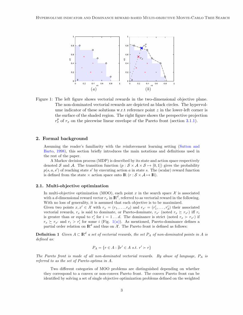
Figure 1: The left figure shows vectorial rewards in the two-dimensional objective plane.The non-dominated vectorial rewards are depicted as black circles. The hypervol-ume indicator of these solutions w.r.t reference point z in the lower-left corner isthe surface of the shaded region. The right figure shows the perspective projectionrpx of rx on the piecewise linear envelope of the Pareto front (section 3.1.1).

2. Formal background

Assuming the reader’s familiarity with the reinforcement learning setting (Sutton andBarto, 1998), this section briefly introduces the main notations and definitions used inthe rest of the paper.

A Markov decision process (MDP) is described by its state and action space respectivelydenoted S and A. The transition function (p : S × A × S 7→ [0, 1]) gives the probabilityp(s, a, s′) of reaching state s′ by executing action a in state s. The (scalar) reward functionis defined from the state × action space onto IR (r : S ×A 7→ IR).

2.1. Multi-objective optimization

In multi-objective optimization (MOO), each point x in the search space X is associatedwith a d-dimensional reward vector rx in IRd, referred to as vectorial reward in the following.With no loss of generality, it is assumed that each objective is to be maximized.Given two points x, x′ ∈ X with rx = (r1, . . . , rd) and rx′ = (r′1, . . . , r

′d) their associated

vectorial rewards, rx is said to dominate, or Pareto-dominate, rx′ (noted rx � rx′) iff riis greater than or equal to r′i for i = 1 . . . d. The dominance is strict (noted rx � rx′) ifrx � rx′ and ri > r′i for some i (Fig. 1(a)). As mentioned, Pareto-dominance defines apartial order relation on IRd and thus on X . The Pareto front is defined as follows:

Definition 1 Given A ⊂ IRd a set of vectorial rewards, the set PA of non-dominated points in A isdefined as:

PA = {r ∈ A : @r′ ∈ A s.t. r′ � r}

The Pareto front is made of all non-dominated vectorial rewards. By abuse of language, PA isreferred to as the set of Pareto-optima in A.

Two different categories of MOO problems are distinguished depending on whetherthey correspond to a convex or non-convex Pareto front. The convex Pareto front can beidentified by solving a set of single objective optimization problems defined on the weighted

3

Wang Sebag

sum of the objectives, referred to as linear scalarization of the MOO problem (as done inMOQL, section 4.2.1). When dealing with non-convex Pareto fronts (for instance, the DSTproblem (Vamplew et al., 2010), and the ZDT2 and DTLZ2 test benchmarks (Deb et al.,2002)) however, the linear scalarization approach fails to discover the non-convex parts ofthe Pareto front (Deb, 2001). Although many MOO problems have a convex Pareto front,especially in the two-objective case, the discovery of the non-convex Pareto front remainsthe main challenge for MOO approaches (Deb et al., 2000; Beume et al., 2007)1.

2.2. Monte-Carlo Tree Search

Let us describe the best known MCTS algorithm, referred to as Upper Confidence Tree(UCT) (Kocsis and Szepesvari, 2006) and extending the Upper Confidence Bound algorithm(Auer et al., 2002) to tree-structured spaces. UCT simultaneously explores and builds asearch tree, initially restricted to its root node, along N tree-walks a.k.a. simulations. Eachtree-walk involves three phases:The bandit phase starts from the root node and iteratively selects an action/a child nodeuntil arriving in a leaf node. Action selection is handled as a multi-armed bandit problem.The set As of admissible actions a defines the possible child nodes (s, a) of node s; theselected action a∗ maximizes the Upper Confidence Bound:

rs,a +√ce ln(ns)/ns,a (1)

over a ranging in As, where ns stands for the number of times node s has been visited, ns,adenotes the number of times a has been selected in node s, and rs,a is the average rewardcollected when selecting action a from node s. The first (respectively the second) termin Eq. (1) corresponds to the exploitation (resp. exploration) term, and the explorationvs exploitation trade-off is controlled by parameter ce. Upon the selection of a∗, the nextstate is drawn from the transition model depending on the current state and a∗. In theremainder of the paper, a tree node is labeled with the sequence of actions followed fromthe root; the associated reward is the average reward collected over all tree-walks involvingthis node.The tree building phase takes place upon arriving in a leaf node s; some action a is(uniformly or heuristically) selected and (s, a) is added as child node of s. Accordingly, thenumber of nodes in the tree is the number of tree-walks.The random phase starts from the new leaf node (s, a) and iteratively (uniformly orheuristically) selects an action until arriving in a terminal state u; at this point the rewardru of the whole tree-walk is computed and used to update the reward estimates in all nodes(s, a) visited during the tree-walk:

rs,a ←1

ns,a + 1

(ns,a × rs,a + ru

)(2)

ns,a ← ns,a + 1; ns ← ns + 1

Additional heuristics have been considered, chiefly to prevent over-exploration when thenumber of admissible arms is large w.r.t the number of simulations (the so-called many-armed bandit issue (Wang et al., 2008)). The Progressive Widening (PW) heuristics(Coulom, 2006) will be used in the following, where the allowed number of child nodesof s is initialized to 1 and increases with its number of visits ns like bns1/bc (with b usuallyset to 2 or 4). The Rapid Action Value Estimation (RAVE) heuristic is meant to guide theexploration of the search space (Gelly and Silver, 2007). In its simplest version, RAV E(a)

1. Notably, the chances for a Pareto front to be convex decreases with the number of objectives.

4


is set to the average reward taken over all tree-walks involving action a. The RAVE vectorcan be used to guide the tree-building phase2, that is, when selecting a first child node uponarriving in a leaf node s, or when the Progressive Widening heuristics is triggered and anew child node is added to the current node s. In both cases, the selected action is the onemaximizing RAV E(a). The RAVE heuristic aims at exploring earlier the most promisingregions of the search space; for the sake of convergence speed, it is clearly desirable toconsider the best options as early as possible.

3. Overview of MOMCTS

The main difference between MCTS and MOMCTS regards the node selection step. Thechallenge is to extend the single-objective node selection criterion (Eq. (1)) to the multi-objective setting. Since there is no total order between points in the multi-dimensionalspace, as mentioned, the most straightforward way of dealing with multi-objective opti-mization is to get back to single-objective optimization, through aggregating the objectivesinto a single one; the price to pay is that this approach yields a single solution on thePareto front. Two aggregating functions (the hypervolume indicator and the cumulativediscounted dominance reward) aimed at recovering a total order among points in the multi-dimensional reward space conditionally to the search archive, will be integrated within theMCTS framework.The MOMCTS-hv algorithm is presented in section 3.1 and its limitations are discussedin section 3.2. The MOMCTS-dom algorithm aimed at overcoming these limitations isintroduced in section 3.3.

3.1. MOMCTS-hv

3.1.1. Node selection based on hypervolume indicator

The hypervolume indicator (Zitzler and Thiele, 1998) provides a scalar measure of solutionsets in the multi-objective space as follows.

Definition 2 Given A ⊂ IRd a set of vectorial rewards, given reference point z ∈ IRd such that itis dominated by every r ∈ A, then the hypervolume indicator (HV) of A is the measure of the set ofpoints dominated by some point in A and dominating z:

HV (A; z) = µ({x ∈ IRd : ∃r ∈ A s.t. r � x � z})

where µ is the Lebesgue measure on IRd (Fig.1( a)).

It is clear that all dominated points in A can be removed without modifying the hypervol-ume indicator (HV (A; z) = HV (PA; z)). As shown by Fleischer (2003), the hypervolumeindicator is maximized iff points in PA belong to the Pareto front of the MOO problem.Auger et al. (2009) show that, for d = 2, for a number K of points, the hypervolume indi-cator maps a multi-objective optimization problem defined on IRd, onto a single-objectiveoptimization problem on IRd×K , in the sense that there exists at least one set of K pointsin IRd that maximizes the hypervolume indicator w.r.t. z.

Let P denote the archive of non-dominated vectorial rewards measured for every ter-minal state u (section 2.2). It then comes naturally to define the value of any MCTS treenode as follows.

2. Another option is to use a dynamically weighted combination of the reward rs,a and RAV E(a) in Eq.(1).

5

Wang Sebag

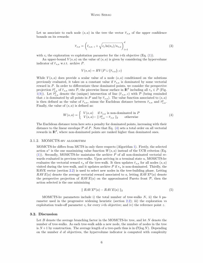
Let us associate to each node (s, a) in the tree the vector rs,a of the upper confidencebounds on its rewards:

rs,a =

(rs,a; i +

√ci ln(ns)/ns,a

)di=1

(3)

with ci the exploration vs exploitation parameter for the i-th objective (Eq. (1)).An upper-bound V (s, a) on the value of (s, a) is given by considering the hypervolume

indicator of rs,a w.r.t. archive P .

V (s, a) = HV (P ∪ {rs,a}; z)

While V (s, a) does provide a scalar value of a node (s, a) conditioned on the solutionspreviously evaluated, it takes on a constant value if rs,a is dominated by some vectorialreward in P . In order to differentiate these dominated points, we consider the perspectiveprojection rps,a of rs,a onto P, the piecewise linear surface in IRd including all ru ∈ P (Fig.1(b)). Let rps,a denote the (unique) intersection of line (rs,a, z) with P (being remindedthat z is dominated by all points in P and by rs,a). The value function associated to (s, a)is then defined as the value of rs,a, minus the Euclidean distance between rs,a and rps,a.Finally, the value of (s, a) is defined as:

W (s, a) =

{V (s, a) if rs,a is non-dominated in PV (s, a)− ‖ rps,a − rs,a ‖2 otherwise

(4)

The Euclidean distance term here sets a penalty for dominated points, increasing with theirdistance to the linear envelope P of P . Note that Eq. (4) sets a total order on all vectorialrewards in IRd, where non-dominated points are ranked higher than dominated ones.

3.1.2. MOMCTS-hv algorithm

MOMCTS-hv differs from MCTS in only three respects (Algorithm 1). Firstly, the selectedaction a∗ is the one maximizing value function W (s, a) instead of the UCB criterion (Eq.(1)). Secondly, MOMCTS-hv maintains the archive P of all non-dominated vectorial re-wards evaluated in previous tree-walks. Upon arriving in a terminal state u, MOMCTS-hvevaluates the vectorial reward ru of the tree-walk. It then updates rs,a for all nodes (s, a)visited during the tree-walk, and it updates archive P if ru is non-dominated. Thirdly, theRAVE vector (section 2.2) is used to select new nodes in the tree-building phase. LettingRAV E(a) denote the average vectorial reward associated to a, letting RAV Ep(a) denotethe perspective projection of RAV E(a) on the approximated Pareto front P, then theaction selected is the one minimizing

‖ RAV Ep(a)−RAV E(a) ‖2 (5)

MOMCTS-hv parameters include i) the total number of tree-walks N , ii) the b pa-rameter used in the progressive widening heuristic (section 2.2); iii) the exploration vsexploitation trade-off parameter ci for every i-th objective; and iv) the reference point z.

3.2. Discussion

Let B denote the average branching factor in the MOMCTS-hv tree, and let N denote thenumber of tree-walks. As each tree-walk adds a new node, the number of nodes in the treeis N+1 by construction. The average length of a tree-path thus is in O(logN). Dependingon the number d of objectives, the hypervolume indicator is computed with complexity

6


Algorithm 1 MOMCTS-hv

MOMCTS-hvInput: number N of tree-walksOutput: search tree TInitialize T ← root node (initial state), P ← {}for t = 1 to N do

TreeWalk(T , P, root node)end forreturn T

TreeWalkInput: search tree T , archive P , node sOutput: vectorial reward ruif s is not a leaf node, and ¬(b(ns + 1)1/bc > b(ns)1/bc) // (PW test is not triggered)then

Select a∗ = argmax {W (s, a), (s, a) ∈ T } //Eq. (4)ru ← TreeWalk(T , P, (s, a∗))

elseAs = { admissible actions not yet visited in s}Select a∗ = arg min{‖ RAV Ep(a)−RAV E(a) ‖2, a ∈ As}Add (s, a∗) as child node of sru ← RandomWalk(P, (s, a∗))

end ifUpdate ns, ns,a∗ , RAV E(a∗) and rs,areturn ru

RandomWalkInput: archive P , state uOutput: vectorial reward ruArnd ← {} // store the set of actions visited in the random phasewhile u is not final state do

Uniformly select an admissible action a for uArnd ← Arnd ∪ {a}u← (u, a)

end whileru = evaluate(u) //obtain the vectorial reward of the tree-walkif ru is not dominated by any point in P then

Prune all points dominated by ru in PP ← P ∪ {ru}

end ifUpdate RAV E(a) for a ∈ Arndreturn ru

7

Wang Sebag

O(|P |d/2) for d > 3 (respectively O(|P |) for d = 2 and O(|P | log |P |) for d = 3) (Beumeet al., 2009). The complexity of each tree-walk thus is O(B|P |d/2logN), where |P | is atmost the number N of tree-walks.

By construction, the hypervolume indicator based selection criterion (Eq. (4)) drivesMOMCTS-hv towards the Pareto front and favours the diversity of the Pareto archive.On the negative side however, the computational cost of W (s, a) is exponential withthe number d of objectives. Besides, the hypervolume indicator is not invariant undermonotonous transformation of objective functions, which prevents the approach from en-joying the same robustness as comparison-based optimization approaches (Hansen, 2006).Lastly, the MOMCTS-hv critically depends on its hyper-parameters. The exploration vsexploitation (EvE) trade-off parameters ci, i = 1, 2, . . . , d (Eq. (1)) of each objective havea significant impact on the performance of MOMCTS-hv (likewise, the MCTS applicativeresults depend on the tuning of the EvE trade-off parameters (Chaslot et al., 2008)). Addi-tionally, the choice of the reference point z also influences the hypervolume indicator values(Auger et al., 2009)).

3.3. MOMCTS-dom

This section presents a new MOMCTS approach aimed at overcoming the above limitations,which is based on the Pareto dominance test. Notably, this test has linear complexity w.r.t.the number of objectives, and is invariant under monotonous transformation of objectives.As this reward depends on the Pareto archive which evolves along the search, the cumulativediscounted dominance(CDD) reward mechanism is proposed to handle the search dynamics.

3.3.1. Node selection based on cumulative discounted dominance reward

Let P denote the archive of all non-dominated vectorial rewards previously gathered duringthe search process. A straightforward option would be to associate to each tree-walk reward1 if the tree-walk gets a vectorial reward ru which is not strictly dominated by any pointin the archive P , and reward 0 otherwise. Formally this boolean dominance reward, calledru;dom, is defined as:

ru;dom =

{1 if @r ∈ P, r � ru0 otherwise

(6)

The optimization problem defined by dominance rewards is non-stationary as it depends onthe archive P , which evolves along time. To cope with non-stationarity, the reward updateproceeds along a cumulative discounted (CD) process as follows. Let ts,a denote the indexof the last tree-walk which visited node (s, a), let ∆t = t− ts,a where t is the index of thecurrent tree-walk, let δ ∈ [0, 1] be a discount factor, the CD update is defined as:

rs,a;dom ← rs,a;dom · δ∆t + ru;dom, δ ∈ [0, 1] (7)

ts,a ← t; ns,a ← ns,a + 1; ns ← ns + 1

The reward update in MOMCTS-dom differs from the standard scheme (Eq. (2)) in tworespects. Firstly, cumulative instead of average rewards are considered. The rationale forthis modification is that a tiny percentage of the tree-walks finds a non-dominated vectorialreward if ever. In such cases, average rewards come to be negligible in front of the explo-ration term, making the MCTS degenerate to pure random search. The use of cumulativerewards instead tends to prevent this degradation.Secondly, a discount mechanism is used to moderate the cumulative effects using the dis-count factor δ (0 ≤ δ ≤ 1) and taking into account the number ∆t of tree-walks since thisnode was last visited. This discount mechanism is meant to cope with the dynamics of

8


multi-objective search through forgetting old rewards, thus enabling the decision rule toreflect up-to-date information.Indeed, the CD process is reminiscent of the discounted cumulative reward defining thevalue function in Reinforcement Learning (Sutton and Barto, 1998), with the differencethat the time-step t here corresponds to the tree-walk index, and that the discount mech-anism is meant to limit the impact of past (as opposed to, future) information.

In a stationary context, rs,a;dom would converge towards 11−δ∆t r, with ∆t the average

interval of time between two visits to the node. If the node gets exponentially rarely visited,rs,a;dom goes to r. Quite the contrary, if the node happens to be frequently visited, r ismultiplied by a large factor ( 1

1−δ ), entailing the over-exploitation of the node. However,the over-exploitation is bound to decrease as soon as the Pareto archive moves towards thetrue Pareto front. While this CDD reward was found to be empirically suited to the MOOsetting (see also Maes et al. (2011)), further work is required to analyze its properties.

3.3.2. MOMCTS-dom algorithm

MOMCTS-dom proceeds as standard MCTS except for the update procedure, where Eq.(2) is replaced by Eq. (7). Keeping the same notations B,N and |P | as above, as thedominance test in the end of each tree-walk is linear (O(d|P |)), the complexity of eachtree-walk in MOMCTS-dom is O(B logN + d|P |), linear w.r.t. the number d of objectives.

Besides the MCTS parameters N and b, MOMCTS-dom involves two additional hyper-parameters: i) the exploration vs exploitation trade-off parameter ce; and ii) the discountfactor δ.

4. Experimental validation

This section presents the experimental validation of the MOMCTS-hv and MOMCTS-domalgorithms.

4.1. Goals of experiments

The first goal is to assess the performance of the MOMCTS approaches comparatively tothe state of the art in MORL (Vamplew et al., 2010). Two artificial benchmark problems(Deep Sea Treasure and Resource Gathering) with probabilistic transition functions areconsidered. The Deep Sea Treasure problem has two objectives which define a non-convexPareto front (section 4.2). The Resource gathering problem has three objectives and aconvex Pareto front (section 4.3). The second goal is to assess the performance and scal-ability of MOMCTS approaches in a real-world setting, that of grid scheduling problems(section 4.4).

All reported results are averaged over 11 runs unless stated otherwise.

Indicators of performance

Two indicators are defined to measure the quality of solution sets in the multi-dimensionalspace. The first indicator is the hypervolume indicator (section 3.1.1). The second indi-cator, inspired from the notion of regret, is defined as follows. Let P ∗ denote the truePareto front. The empirical Pareto front P defined by a search process is assessed fromits generational distance (Van Veldhuizen, 1999) and inverted generational distance w.r.t.

P ∗. The generational distance (GD) is defined by GD(P ) =(√∑n

i=1 d2i

)/n, where n is

the size of P and di is the Euclidean distance between the i-th point in P and its nearestpoint in P ∗. GD measures the average distance from points in P to the Pareto front. The

9

Wang Sebag

(a) The state space (b) The Pareto front

Figure 2: The Deep Sea Treasure problem. Left: the DST state space with black cells assea-floor, gray cells as terminal states, the treasure value is indicated in eachcell. The initial position is the upper left cell. Right: the Pareto front in thetime×treasure plane.

inverted generational distance (IGD) is likewise defined as the average distance of pointsin P ∗ to their nearest neighbour in P . For both generational and inverted generationaldistances, the smaller, the better.

The algorithms are also assessed w.r.t. their computational cost (measured on a PCwith Intel dual-core CPU 2.66GHz).

4.2. Deep Sea Treasure

The Deep Sea Treasure (DST) problem, first introduced by Vamplew et al. (2010), isconverted into a stochastic sequential decision making problem by introducing noise in thetransition function of DST. The state space of Deep Sea Treasure (DST) consists of a 10×11grid (Fig. 2(a)). The action space of DST includes four actions (up, down, left and right),each sending the agent to one adjacent square in the indicated direction with probability1−η, and in the other three directions with equal probability η/3, where 0 ≤ η < 1 indicatesthe noise level in the environment. When the selected action would send the agent beyondthe grid or the sea borders, the agent stays in the same place. Each policy, with the topleft square as initial state, gets a two dimensional reward: the time spent until reachinga terminal state or reaching the time horizon T = 100, and the treasure attached to theterminal state (Fig. 2(a)). The list of all 10 non-dominated vectorial rewards in the formof (−time, treasure) are depicted in the two-dimensional plane in Fig. 2(b). It is worthnoting that the Pareto front is non-convex.

4.2.1. Baseline algorithm

As mentioned in the introduction, the state of the art in MORL considers a scalar aggrega-tion (e.g. a weighted sum) of rewards associated to all objectives. Several multiple-policyMORL algorithms have been proposed (Natarajan and Tadepalli, 2005; Tesauro et al.,2007; Barrett and Narayanan, 2008; Lizotte et al., 2012) using the weighted sum of the

10


objectives (with several weight settings) as scalar reward, which is optimized using stan-dard reinforcement learning algorithms. The differences between the above algorithms arehow they share the information between different weight settings and which weight settingsthey choose to optimize. In the following, MOMCTS-dom is compared to Multi-ObjectiveQ-Learning (MOQL) (Vamplew et al. (2010)). Choosing MOQL as baseline is motivatedas it yields all policies found by other linear-scalarisation based approaches, provided thata sufficient number of weight settings be considered.

Formally, in the two objective reinforcement learning case, MOQL optimizes indepen-dently m scalar RL problems through Q-learning, where the i-th problem considers rewardri = (1−λi)×ra+λi×rb, where 0 ≤ λi ≤ 1, i = 1, 2, . . . ,m define the m weight settings ofMOQL, and ra (respectively rb) is the first (resp. the second) objective reward. In its sim-plest version, the overall computational effort is equally divided between the m scalar RLproblems. The computational effort allocated to the each weight setting is further equallydivided into ntr training phases; after the j-th training phase, the performance of the i-th weight setting is measured by the two-dimensional vectorial reward, noted ri,j , of thecurrent greedy policy. The m vectorial rewards of all weight settings {r1,j , r2,j , . . . , rm,j}together compose the Pareto front of MOQL at training phase j.

4.2.2. Experimental setting

We use the same MOQL experimental setting as in Vamplew et al. (2010):

• ε-greedy exploration is used with ε = 0.1.

• Learning rate α is set to 0.1.

• The state-action value table is optimistically initialized (time = 0, treasure = 124).

• Due to the episodic nature of DST, no discounting is used in MOQL(γ = 1).

• The number m of weight settings ranges in {3, 7, 21}, with λi = i−1m−1 , i = 1, 2, . . . ,m.

After a few preliminary experiments, the progressive widening parameters b is set to 2 inboth MOMCTS-hv and MOMCTS-dom. In MOMCTS-hv, the exploration vs exploitation(EvE) trade-off parameters in the time cost and treasure value objectives are respectively setto ctime = 20, 000 and ctreasure = 150. As the DST problem is concerned with minimizingthe search time (maximizing its opposite) and maximizing the treasure value, the referencepoint used in the hypervolume indicator calculation is set to (-100,0).In MOMCTS-dom, the EvE trade-off parameter ce is set to 1, and the discount factor δ isset to 0.999.

Experiments are carried out in a DST simulator with the η noise level ranging in 0,1 × 10−3, 1 × 10−2, 5 × 10−2 and 0.1. The training time of MOQL, MOMCTS-hv andMOMCTS-dom is limited to 300,000 time steps (ca 37,000 tree-walks in MOMCTS-hv and45,000 tree-walks in MOMCTS-dom). The entire training process is equally divided intontr = 150 phases. At the end of each training phase, the MOQL and MOMCTS solutionsets are tested in the DST simulator, and form the Pareto set P . The performance ofalgorithms is reported as the hypervolume indicator of P .

4.2.3. Results

Table 1 shows the performance of MOMCTS approaches and MOQL measured by thehypervolume indicator, with reference point z = (−100, 0).

11

Wang Sebag

(a)

(b)

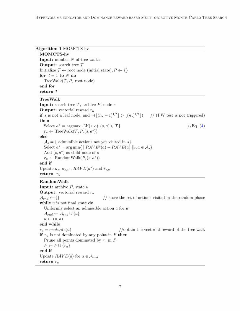
Figure 3: The hypervolume indicator performance of MOMCTS-hv, MOMCTS-dom andMOQL versus training time in the deterministic DST problem (η = 0). For thesake of comparison with MOQL, the training time refers to the number of actionselections in MOMCTS approaches, and each tree-walk in MOMCTS carries outon average 7 to 8 action selections in the DST problem. Top: The hypervolumeindicator of MOMCTS-hv, MOMCTS-dom and MOQL-m=21. Bottom: Thehypervolume indicator of MOQL with m = 3, 7, 21.

12


Table 1: The DST problem: hypervolume indicator results of MOMCTS-hv, MOMCTS-dom and MOQL with m ranging in 3,7 and 21 in with different noise levels η,averaged over 11 independent runs. The optimal hypervolume indicator is 10455.For each η, significantly better results are indicated in bold font (significance valuep < 0.05 for the Student’s t-test).

η = 0 η = 1× 10−3 η = 0.01 η = 0.05 η = 0.1

MOMCTS-hv 10416±37 10434±31 10436±32 10205±211 9883±1091

MOMCTS-dom 10450±4 10446±19 10389±65 9858±1153 9982±360

MOQL-m=3 7099±3926 8116±3194 6422± 4353 7333±4411 6953±3775

MOQL-m=7 10078±34 10049±94 9495±1701 8345±2887 8924±2663

MOQL-m=21 10078±17 10085±129 7806±1933 8744±2070 6744±2355

Deterministic setting

Fig. 3 displays the hypervolume indicator performance of MOMCTS-hv, MOMCTS-domand that of MOQL for m = 3, 7, 21 in the deterministic setting (η = 0). It is observed thatfor m = 7 or 21, MOQL reaches a performance plateau (10062) within 20,000 time steps.The fact that MOQL does not reach the optimal hypervolume indicator 10455 is explainedas the DST Pareto front is not convex (Fig. 2(b)). As widely known (Deb, 2001), linear-scalarisation based approaches of MOO fail to discover solutions in non-convex regions ofthe Pareto front. In such cases, MOQL is prevented from finding the true Pareto frontand thus is inconsistent. Ultimately, MOQL only discovers the extreme points (-19,124)and (-1,1) of the Pareto front (Fig. 4(a)). In the meanwhile, MOMCTS-hv performancedominates that of MOQL throughout the training process. MOMCTS-dom catches upMOQL after 80,000 time steps. The entire Pareto front is found by MOMCTS-hv in 5 out11 runs, and by MOMCTS-dom algorithm in 10 out 11 runs.

Fig. 3(b) shows the influence of m on MOQL. For m = 7, MOQL reaches the perfor-mance plateau before m = 21 (respectively 8,000 time steps vs 20,000 time steps), albeitwith some instability. The instability increases as m is set to 3. The fact that for MOQL-m = 3 fails to reach the MOQL performance plateau is explained as the extreme point(-19,124) can be missed in some runs as MOQL uses a discount factor of 1 (after Vamplewet al. (2010)). Therefore the largest 124 treasure might be discovered later than in timestep 19.

The percentage of times out of 11 runs that each non-dominated vectorial rewardis discovered for at least one test episode during the training process of MOMCTS-hv,MOMCTS-dom and MOQL for m = 21 is displayed in Fig. 4(b). This picture showsthat MOQL discovers all strategies (lying in the non-convex regions of the Pareto front)during intermediate test episodes. However, these non-convex strategies are eventuallydiscarded as the MOQL solution set gradually converges to extreme strategies. Quitethe contrary, MOMCTS approaches discovers all strategies in the Pareto front, and keepsthem in the search tree after they have been discovered. The weakness of MOMCTS-hvis that the longest decision sequences corresponding to the vectorial rewards (-17,74) and(-19,124) need more time to be discovered. The MOMCTS-dom successfully discovers allnon-dominated vectorial rewards (in 10 out of 11 runs) and reaches an average hypervolumeindicator performance slightly higher than that of MOMCTS-hv.

13

Wang Sebag

(a) (b)

Figure 4: Left: The vectorial rewards found by representative MOMCTS-hv, MOMCTS-dom and MOQL-m = 21 runs. Right: The percentage of times out of 11runs that each non-dominated vectorial reward was discovered by MOMCTS-hv,MOMCTS-dom and MOQL-m = 21, during at least one test episode.

Stochastic setting

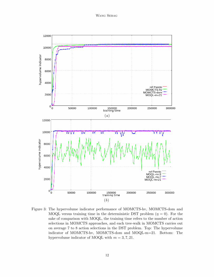
Fig. 5 shows the performance of MOMCTS-hv, MOMCTS-dom and MOQL-m=21 in thestochastic environments (η = 0.01, 0.1). As could have been expected, the performancesof MOQL and MOMCTS approaches decrease and their variances increase with noise levelη, although their performances improve with training time (except for the MOQL in theη = 0.01 case). In the low noise case (η = 0.01), MOQL reaches its optimal performanceafter time step 40,000, with a high performance variance. It is outperformed by MOMCTS-hv and MOMCTS-dom, with higher average hypervolume indicators and lower variances.When the noise rate increases (η = 0.1), both performances are degraded while MOMCTSapproaches still outperforms MOQL in terms of relative performance and lower variance(as shown in Table 1), showing a good robustness w.r.t. noise.

In summary, the empirical validation on the artificial DST problem shows both thestrengths and the weaknesses of MOMCTS approaches. On the positive side, MOMCTSapproaches show able to find solutions lying in the non-convex regions of the Pareto front,as opposed to linear scalarization-based methods. Moreover, MOMCTS shows a relativelygood robustness w.r.t. noise. On the negative side, MOMCTS approaches are more com-putationally expensive than MOQL (for 300,000 time steps, MOMCTS-hv takes 147 secs,MOMCTS-dom takes 49 secs versus 25 secs for MOQL).

4.3. Resource Gathering

The Resource Gathering (RG) task first introduced in Barrett and Narayanan (2008) iscarried out in a 5× 5 grid (Fig. 6). The action space of RG include the same four actions(up, down, left and right) as in the DST problem. Starting from the home location, the goalof the agent is to gather two resources (gold and gems) and take them back home. Eachtime the agent reaches one resource location, the resource is picked up. Both resources canbe carried by the agent at the same time. If the agent steps on one of the two enemy cases

14


(a) η = 0.01

(b) η = 0.1

Figure 5: The hypervolume indicator of MOMCTS-hv, MOMCTS-dom and MOQL-m=21versus training time in the stochastic environment (η = 0.01, 0.1).

15

Wang Sebag

Figure 6: The Resource Gathering problem. The initial position of the agent is markedby the home symbol. Two resources (gold and gems) are located in fixed posi-tions. Two enemy cases (marked by swords) send the agent back home with 10%probability.

(indicated by swords), it may be attacked with 10% probability, in which case the agentloses all resources being carried and is returned to the home location immediately. Theagent enters a terminal state when it returns home (including the case of being attacked)or when the time horizon T = 100 is reached. Five possible immediate reward vectorsordered as (enemy, gold, gems) will be received upon the termination of a policy:

• (−1, 0, 0) in case of an enemy attack;

• (0, 1, 0) for returning home with only gold;

• (0, 0, 1) for returning home with only gems;

• (0, 1, 1) for returning home with both gold and gems;

• (0, 0, 0) in all other cases.

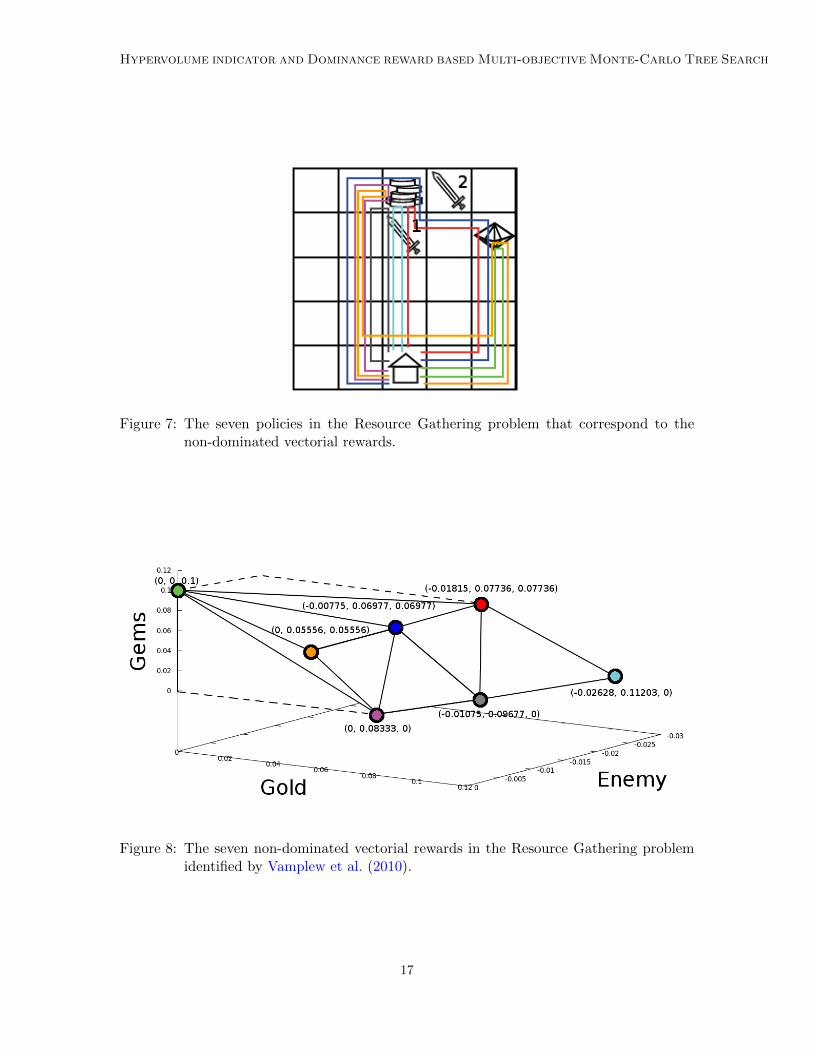
The RG problem contains a discrete state space of 100 states corresponding to the 25 agentpositions in the grid, multiplied by the four possible states of resources currently being held(none, gold only, gems only, both gold and gems). The vectorial reward associated to eachpolicy π is calculated as follows:Let r = (enemy, gold, gems) be the vectorial reward obtained by policy π after a L-stepepisode. The immediate reward of π is set to rπ;L = r/L = (enemy/L, gold/L, gems/L),and the policy is associated its immediate reward averaged over 100 episodes, favoring thediscovery of policies with shortest length. Seven policies (Table 2 and Fig. 7) correspond-ing to the non-dominated average vectorial rewards of the RG problem are identified byVamplew et al. (2010). The non-dominated vectorial rewards compose a convex Paretofront in the three dimensional space (Fig. 8).


In the RG problem, the MOMCTS approaches are assessed comparatively with the MOQLalgorithm, which independently optimizes the weighted sums of the three objective func-

16


Figure 7: The seven policies in the Resource Gathering problem that correspond to thenon-dominated vectorial rewards.

Figure 8: The seven non-dominated vectorial rewards in the Resource Gathering problemidentified by Vamplew et al. (2010).

17

Wang Sebag

Table 2: The optimal policies for the Resource Gathering problem.# policy description vectorial reward

π1 Go directly to gems, avoiding enemies (0,0,0.1)

π2 Go to both gold and gems, avoiding enemies (0, 5.556× 10−2, 5.556× 10−2)

π3 Go directly to gold, avoiding enemies (0, 8.333× 10−2, 0)

π4 Go to both gold and gems, through enemy1 or enemy2 once (−7.75× 10−3, 6.977× 10−2, 6.977× 10−2)

π5 Go directly to gold, through enemy1 once (−1.075× 10−2, 9.677× 10−2, 0)

π6 Go to both gold and gems, through the enemies twice (−1.815× 10−2, 7.736× 10−2, 7.736× 10−2)

π7 Go directly to gold, through enemy1 twice (−2.628× 10−2, 1.1203× 10−1, 0)

tions (enemy, gold, gems) under m weight settings. In the three dimensional rewardspace, one weight setting is defined by a 2D vector (λi, λ

′j), with λi, λ

′j ∈ [0, 1] and

0 ≤ λi + λ′j ≤ 1. Let us denote the scalar rewards optimized by MOQL as ri,j =(1 − λi − λ′j) × renemy + λi × rgold + λ′j × rgems, where l weights λi (respectively λ′j)are evenly distributed in [0, 1] for the gold (resp. gems) objective, subject to λi + λ′j ≤ 1,

the total number of weight settings thus is m = l(l−1)2 .

The parameters of MOQL and MOMCTS approaches have been selected after prelimi-nary experiments, using the same amount of computational resources for a fair comparison.For the MOQL:

• The ε-greedy exploration is used with ε = 0.2.

• Learning rate α is set to 0.2.

• The discount factor γ is set to 0.95.

• By taking l = 4, 6, 10, the number m of weight settings ranges in {6, 15, 45}.

In MOMCTS-hv, the progressive widening parameter b is set to 2. The explorationvs exploitation (EvE) trade-off parameters associated to each objective are defined ascenemy = 1 × 10−3, cgold = 1 × 10−4, cgems = 1 × 10−4. The reference point z used inthe hypervolume indicator calculation is set to (−0.33,−1× 10−3,−1× 10−3), where -0.33represents the maximum enemy penalty averaged in each time step of the episode, and the−1 × 10−3 values in the gold and gems objectives are taken to encourage the explorationof solutions with vectorial rewards lying in the hyper-planes gold = 0 and gems = 0.In MOMCTS-dom, the progressive widening parameter b is set to 1 (no progressive widen-ing). The EvE trade-off parameter ce is set to 0.1. The discount factor δ is set to 0.99.

The training time of all considered algorithms is 600,000 time steps (ca 17,200 tree-walksfor MOMCTS-hv and 16,700 tree-walks for MOMCTS-dom). Like in the DST problem,the training process is equally divided into 150 phases. At the end of each training phase,the MOQL and MOMCTS solution sets are tested in the RG simulator. Each solution(strategy) is launched 100 times and is associated the average vectorial reward (which mightdominate the theoretical optimal ones due to the limited sample). The vectorial rewardsof the solution set provided by each algorithm defines its Pareto archive. The algorithmperformance is set to the hypervolume indicator of the Pareto archive with reference pointz = (−0.33,−1× 10−3,−1× 10−3). The optimal hypervolume indicator is 2.01× 10−3.

4.3.2. Results

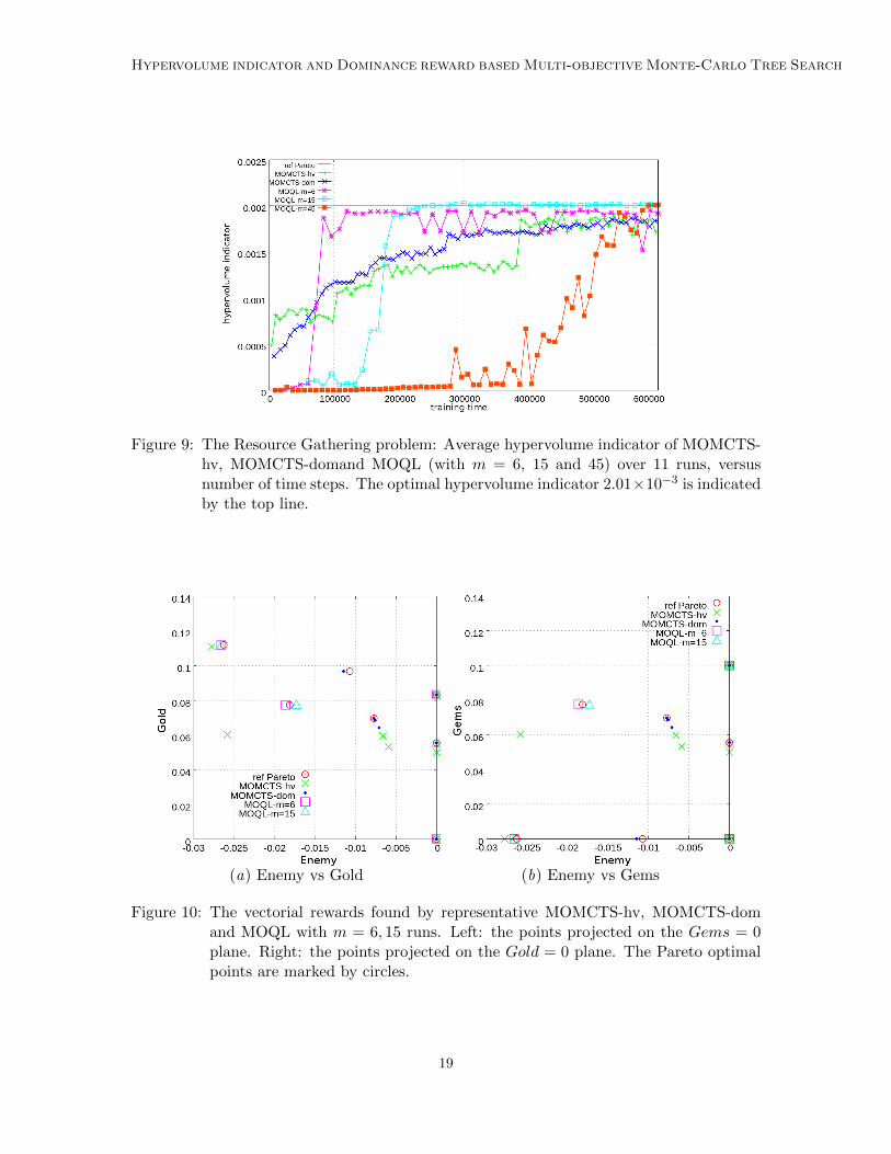
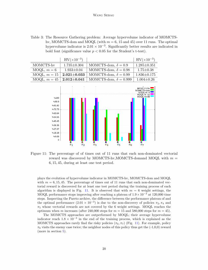
Table 3 shows the performance of MOMCTS-hv, MOMCTS-dom and MOQL algorithmsafter 600,000 times steps of training, measured by the hypervolume indicator. Fig. 9 dis-

18


Figure 9: The Resource Gathering problem: Average hypervolume indicator of MOMCTS-hv, MOMCTS-domand MOQL (with m = 6, 15 and 45) over 11 runs, versusnumber of time steps. The optimal hypervolume indicator 2.01×10−3 is indicatedby the top line.

(a) Enemy vs Gold (b) Enemy vs Gems

Figure 10: The vectorial rewards found by representative MOMCTS-hv, MOMCTS-domand MOQL with m = 6, 15 runs. Left: the points projected on the Gems = 0plane. Right: the points projected on the Gold = 0 plane. The Pareto optimalpoints are marked by circles.

19

Wang Sebag

Table 3: The Resource Gathering problem: Average hypervolume indicator of MOMCTS-hv, MOMCTS-dom and MOQL (with m = 6, 15 and 45) over 11 runs. The optimalhypervolume indicator is 2.01× 10−3. Significantly better results are indicated inbold font (significance value p < 0.05 for the Student’s t-test).

HV(×10−3) HV(×10−3)

MOMCTS-hv 1.735±0.304 MOMCTS-dom, δ = 0.9 1.285±0.351

MOQL, m = 6 1.933±0.04 MOMCTS-dom, δ = 0.98 1.75±0.38



Figure 11: The percentage of of times out of 11 runs that each non-dominated vectorialreward was discovered by MOMCTS-hv,MOMCTS-domand MOQL with m =6, 15, 45, during at least one test period.

plays the evolution of hypervolume indicator in MOMCTS-hv, MOMCTS-dom and MOQLwith m = 6, 15, 45. The percentage of times out of 11 runs that each non-dominated vec-torial reward is discovered for at least one test period during the training process of eachalgorithm is displayed in Fig. 11. It is observed that with m = 6 weight settings, theMOQL performance stops improving after reaching a plateau of 1.9×10−3 at 120,000 timesteps. Inspecting the Pareto archive, the difference between the performance plateau of andthe optimal performance (2.01 × 10−3) is due to the non-discovery of policies π2, π4 andπ5 whose vectorial rewards are not covered by the 6 weight settings. MOQL reaches theoptimum when m increases (after 240,000 steps for m = 15 and 580,000 steps for m = 45).

The MOMCTS approaches are outperformed by MOQL; their average hypervolumeindicator reach 1.8 × 10−3 in the end of the training process, which is explained as theMOMCTS approaches rarely find the risky policies (π6, π7) (Fig. 11). For example, policyπ6 visits the enemy case twice; the neighbor nodes of this policy thus get the (-1,0,0) reward(more in section 5).

20


Figure 12: The hypervolume indicator performance of MOMCTS-dom with δ varying in{0.9, 0.98, 0.99, 0.999}, versus training time steps in the Resource Gatheringproblem.

Figure 13: The Resource Gathering problem: average computational cost for one tree-walkfor MOMCTS-hv and MOMCTS-dom over 11 independent runs. On average,each tree-walk in MOMCTS is ca. 35 training time steps.

As shown in Fig. 12, the δ parameter governs the MOMCTS-dom performance. A lowvalue (δ = 0.9) leads to quickly forgetting the discovery of non-dominated rewards, turningMOMCTS-dom into pure exploration. Quite the contrary, high values of δ (δ = 0.999)limit the exploration and likewise hinder the overall performance.

On the computational cost side, the average execution time of 600,000 training stepsof in MOMCTS-hv, MOMCTS-dom and MOQL are respectively 944 secs, 47 secs and 43secs. As the size of the Pareto archive is close to 10 in most tree-walks of MOMCTS-hv and

21

Wang Sebag

(a) (b)

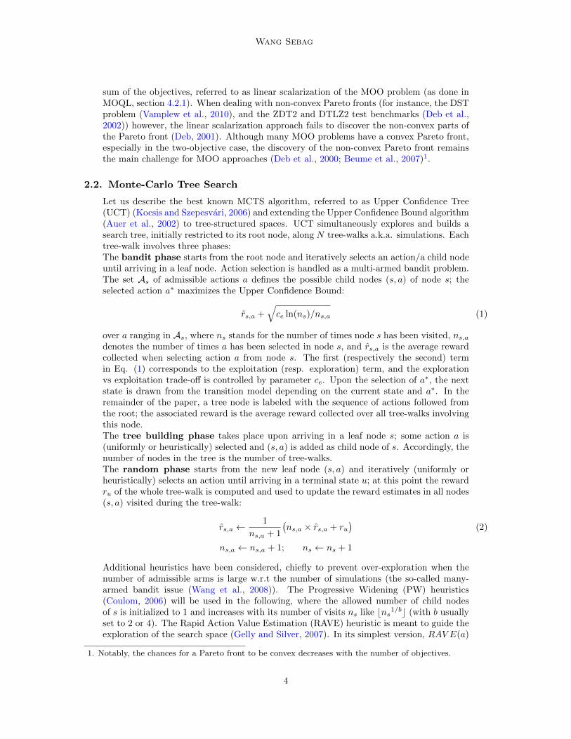
Figure 14: Scheduling a job containing 7 interdependent tasks on a grid of 2 resources.Left: The dependency graph of tasks in the job. Right: The illustration of anexecution plan.

MOMCTS-dom, the fact that MOMCTS-hv algorithm is 20 times slower than MOMCTS-dom matches their computational complexities.As shown in Fig. 13, the cost of tree-walks in MOMCTS-hv increases up to 20 timeshigher than that of MOMCTS-dom within the first 500 tree-walks, during which periodthe Pareto archive size |P | grows. Afterwards, the cost of MOMCTS-hv gradually increaseswith the depth of the search tree (O(logN)). On the contrary, the computational cost ofeach tree-walk in MOMCTS-dom remains stable (between 1×10−3 secs and 2×10−3 secs)throughout the training process.

4.4. Grid scheduling

Pertaining to the domain of autonomic computing (Tesauro et al., 2007), the problem ofgrid scheduling has been selected to investigate the scalability of MOMCTS approaches.The presented experimental validation considers the problem of grid scheduling, referringthe reader to Yu et al. (2008) for a comprehensive presentation of the field. Grid schedulingat large is concerned with scheduling the different tasks involved in the jobs on differentcomputational resources. As tasks are interdependent and resources are heterogeneous,grid scheduling defines an NP-hard combinatorial optimization problem (Ullman (1975)).

Grid scheduling naturally aims at minimizing the so-called makespan, that is the over-all job completion time. But other objectives such as energy consumption, monetary cost,or the allocation fairness w.r.t. the resource providers become increasingly important. Inthe rest of section 4.4, two objectives will be considered, the makespan and the cost of thesolution.

In grid scheduling, a job is composed of J tasks T1 . . . TJ , partially ordered through adependency relation; Ti → Tj denotes that task Ti must be executed before task Tj (Fig.14(a)). Each task Ti is associated with its unitary load Li. Each task is assigned one out ofM resources R1, . . . RM ; resource Rk has computational efficiency speedk and unitary costcostk. Grid scheduling achieves the task-resource assignment and orders the tasks executedon each resource. A grid scheduling solution called execution plan is given as a sequence σof (task-resource) pairs (Fig. 14(b)).

22


Let ρ(i) = k denote the index of the resource Rk on which Ti is executed. Let B(Ti)denote the set of tasks Tj which must either be executed before Ti (Tj → Ti) or which arescheduled to take place before Ti on the same resource Rρ(i). The completion time of atask Ti is recursively computed as:

end(Ti) =Li

speedρ(i)+max{end(Tj), Tj ∈ B(Ti)}

where the first term is the time needed to process Ti on the assigned resource Rρ(i), and thesecond term expresses the fact that all jobs in B(Ti) must be completed prior to executingTi.Finally, grid scheduling is the two-objective optimization problem aimed at minimizing theoverall scheduling makespan and cost:

Find (σ) = argmin {max{end(Tj), j = 1 . . . J} ;∑k=1...M

costkspeedk

×∑i s.t. ρ(i)=k Li}

4.4.1. Baseline algorithms

The state of the art in grid scheduling is achieved by stochastic optimization algorithms(Yu et al., 2008). The two prominent multi-objective variants thereof are NSGA-II (Debet al., 2000) and SMS-EMOA (Beume et al., 2007).Both algorithms can be viewed as importance sampling methods. They maintain a popula-tion of solutions, initially defined as random execution plans. Iteratively, the solutions withbest Pareto rank and best crowded distance (a density estimation of neighboring points inNSGA-II) or hypervolume indicator (in SMS-EMOA) are selected and undergo unary andbinary stochastic perturbations.


A simulated grid environment containing 3 resources with different unit time costs and pro-cessing capabilities (cost1 = 20, speed1 = 10; cost2 = 2, speed2 = 5; cost3 = 1, speed3 = 1)is defined. We firstly compare the performance of MOMCTS approaches and baseline algo-rithms on a realistic bio-informatic workflow EBI ClustalW2, which performs a ClustalWmultiple sequence alignment using the EBI’s WSClustalW2 service3. This workflow con-tains 21 tasks and 23 precedence pairs (graph density q = 12%), assuming that all workloadsare equal. Secondly, the scalability of MOMCTS approaches is tested through experimentsbased on artificially generated workflows containing respectively 20, 30 and 40 tasks withgraph density q = 15%.

As evidenced from the literature (Wang and Gelly (2007)), MCTS performances heav-ily depend on the so-called random phase (section 2.2). Preliminary experiments showedthat a uniform action selection in the random phase was ineffective. A simple heuristicwas thus used to devise a better suited action selection criterion in the random phase, asfollows.Let EFTi define the expected finish time of task Ti (computed off-line):

EFTi = Li +max{EFTj s.t. Tj → Ti}

The heuristic action selection uniformly selects an admissible task Ti. It then comparesEFTi to all EFTj for Tj admissible. If EFTi is maximal, Ti is allocated to the resource

3. The complete description is available at http://www.myexperiment.org/workflows/203.html.

23

Wang Sebag

which is due to be free at the earliest; if EFTi is minimal, Ti is allocated to the resourcewhich is due to be free at the latest. The random phase thus implements a default policy,randomly allocating tasks to resources, except for the most (respectively less) critical tasksthat are scheduled with high (resp. low) priority.

The parameters of all algorithms have been selected after preliminary experiments,using the same amount of computational resources for a fair comparison. The progressivewidening parameter b is set to 2 in both MOMCTS-hv and MOMCTS-dom. In MOMCTS-hv, the exploration vs. exploitation (EvE) trade-off parameters associated to the makespanand cost objectives, ctime and ccost are both set to 5× 10−3. In MOMCTS-dom, the EvEtrade-off parameters ce is set to 1, and the discount factor δ is set to 0.99. The parametersused for NSGA-II (respectively SMS-EMOA) involve a population size of 200 (resp. 120)individuals, of which 100 are selected and undergo stochastic unary and binary variations(resp. one-point re-ordering, and resource exchange among two individuals). For all threealgorithms, the number N of tree-walks a.k.a. evaluation budget is set to 10,000. Thereference point in each experiment is set to (zt, zc), where zt and zc respectively denote themaximal makespan and cost.

Due to the lack of the true Pareto front in the considered problems, we use a referencePareto front P ∗ gathering all non-dominated vectorial rewards obtained in all runs of allthree algorithms to replace the true Pareto front. The performance indicators are definedby the generational distance (GD) and inverted generational distance (IGD) between theactual Pareto front P found in the run and the reference Pareto front P ∗. In the gridscheduling experiment, the IGD indicator plays a similar role as the hypervolume indicatorin DST and RG problems.

4.4.3. Results

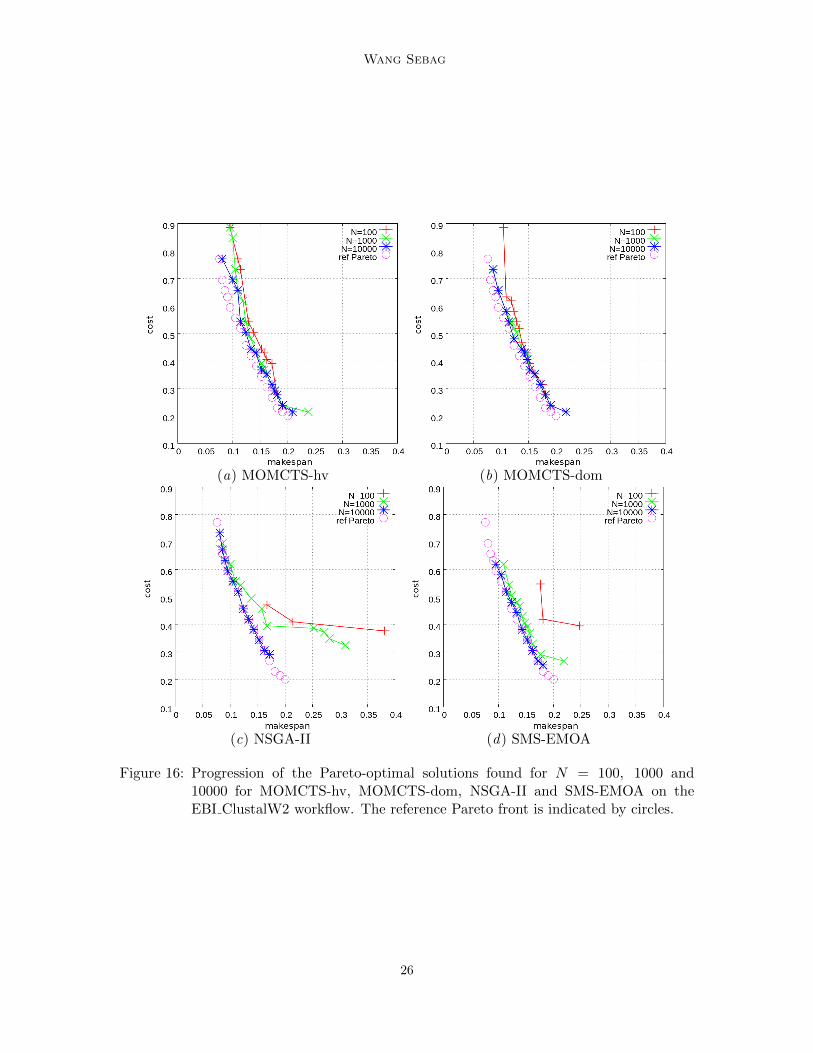
Fig. 15 displays the GD and IGD of MOMCTS-hv, MOMCTS-dom, NSGA-II and SMS-EMOA on EBI ClustalW2 workflow scheduling and on artificial jobs with a number J oftasks ranging in 20, 30 and 40 with graph density q = 15%. Fig. 16 shows the Paretofront discovered by MOMCTS-hv, MOMCTS-dom, NSGA-II and SMS-EMOA on theEBI ClustalW2 workflow after N = 100, 1000 and 10000 policy evaluations (tree-walks),comparatively to the reference Pareto front. In all considered problems, the MOMCTSapproaches are outperformed by the baselines in terms of the GD indicator, while theyquickly find good solutions, they fail to discover the reference Pareto front. In the mean-while, they yield a better IGD performance than the baselines, indicating that on average asingle run of MOMCTS approaches reaches a better approximation of the true Pareto front.

Overall, the main weakness of MOMCTS approaches is their computational runtime.The computational cost of MOMCTS-hv and MOMCTS-dom are respectively 5 and 2.5times higher than that of NSGA-II and SMS-EMOA4. This weakness should have beenrelativized, noting that in real-world problems, the evaluation cost dominates by severalorders of magnitude the search cost.

5. Discussion

As mentioned, the state of the art in MORL is divided into single-policy and multiplepolicy algorithms (Vamplew et al., 2010). In the former case, the authors use a set ofpreferences between objectives which are user-specified or derived from the problem domain

4. On workflow EBI ClustalW2, the average execution time of MOMCTS-hv, MOMCTS-dom, NSGA-IIand SMS-EMOA are respectively 142 secs, 74 secs, 31 secs and 32 secs.

24


(a) EBI ClustalW2 (b) J = 20, q = 15%

(c) J = 30, q = 15% (d) J = 40, q = 15%

Figure 15: The generational distance (GD) and inverted generational distance (IGD) forN = 100, 1000 and 10000 of MOMCTS-hv, MOMCTS-dom, NSGA-II andSMS-EMOA on (a): EBI ClustalW2; (b)(c)(d): artificial problems with numberof tasks J and graph density q. Each performance point after 1000 and 10 000evaluations are respectively marked by single and double cycles.

25

Wang Sebag

(a) MOMCTS-hv (b) MOMCTS-dom

(c) NSGA-II (d) SMS-EMOA

Figure 16: Progression of the Pareto-optimal solutions found for N = 100, 1000 and10000 for MOMCTS-hv, MOMCTS-dom, NSGA-II and SMS-EMOA on theEBI ClustalW2 workflow. The reference Pareto front is indicated by circles.

26


(e.g. defining preferred regions (Mannor and Shimkin, 2004) or setting weights on theobjectives (Tesauro et al., 2007)) to aggregate the multiple objectives in a single one. Thestrength of the single-policy approach is its simplicity; its long known limitation is that itcannot discover a policy in non-convex regions of the Pareto front (Deb, 2001).

In the multiple-policy case, multiple Pareto optimal vectorial rewards can be obtainedby optimization of different scalarized RL problems under different weight settings. Natara-jan and Tadepalli (2005) show that the efficiency of MOQL can be improved by sharinginformation between different weight settings. A hot topic in multiple-policy MORL ishow to design the weight settings and share information among the different scalarized RLproblems. In the case where the Pareto front is known, the design of the weight settingsis made easier − provided that the Pareto front is convex. When the Pareto front is un-known, an alternative provided by Barrett and Narayanan (2008) is to maintain Q-vectorsinstead of Q-values for each pair (state, action). Through an adaptive selection of weightsettings corresponding to the vectorial rewards on the boundary of the convex set of thecurrent Q-vectors, this algorithm narrows down the set of selected weight settings, at theexpense of an higher complexity of value iteration in each state: the O(|S||A|) complexityof standard Q-learning is multiplied by a factor O(nd), where n is the number of points onthe convex hull of the Q-vectors and d is the number of objectives. While the approachprovides optimality guarantees (n converge toward the number of Pareto optimal policies),the number of intermediate solutions can be huge (in the worst case, O(|A||S|)). Basedon the convexity and piece-wise linearity assumption on the shape of the convex hull ofQ-vectors, Lizotte et al. (2012) extends (Barrett and Narayanan, 2008) by narrowing downthe range of points locating on the convex hull, thus keeping the n value under control.

In the MOMCTS-hv approach, each tree node is associated its average reward w.r.t.each objective, and the selection rule involves the scalar associated reward based on thehypervolume indicator (Zitzler and Thiele, 1998), with complexityO(B|P |d/2logN). On theone hand, this complexity is lower than that of a value iteration in Barrett and Narayanan(2008) (considering that the size of archive P is comparable to the number n of non-dominatedQ vectors). On the other hand, this complexity is higher than that of MOMCTS-dom, where the dominance test only needs be computed at the end of each tree-walk, thuswith linear complexity in the number of objectives and tree-walks. The MOMCTS-domcomplexity thus is O(BlogN + d|P |). The price to pay for the improved scalability ofMOMCTS-dom is that the dominance reward might less favor the diversity of the Paretoarchive than the hypervolume indicator: any non-dominated point has the same dominancereward whereas the hypervolume indicator of non-dominated points in sparsely populatedregions of the Pareto archive is higher.

As shown in the Resource Gathering problem, the MOMCTS approaches have dif-ficulties in finding “risky“ policies, visiting nodes with many low reward nodes in theirneighborhood. A tentative explanation for this fact is given as, as already noted by Co-quelin and Munos (2007), it may require an exponential time for the UCT algorithm toconverge to the optimal node if this node is hidden by nodes with low reward.

6. Conclusion and perspectives

This paper has pioneered the extension of MCTS to multi-objective reinforcement learn-ing, based on two scalar rewards measuring the merits of a policy relatively to the non-dominated policies in the search tree. These rewards, respectively the hypervolume in-dicator and the dominance reward, have complementary strengths and weaknesses: thehypervolume indicator is computationally expensive but explicitly favors the diversity ofthe MOO policies, enforcing a good coverage of the Pareto front. Quite the contrary,the dominance test is linear in the number of objectives; it is further invariant under the

27

Wang Sebag

monotonous transformation of the objective functions, a robust property much appreciatedwhen dealing with ill-posed optimization problems.

These approaches have been validated on three problems : Deep Sea Treasure (DST),Resource Gathering (RG) and grid scheduling.

The experimental results on DST confirm a main merit of the proposed approaches,their ability to discover policies lying in the non-convex regions of the Pareto front. To ourknowledge5, this feature is unique in the MORL literature.

In counterpart, MOMCTS approaches suffer from two weaknesses. Firstly, as shown onthe grid scheduling problem, some domain knowledge is required in complex problems toenforce an efficient exploration in the random phase. Secondly, as evidenced in the ResourceGathering problem, the presented approaches hardly discover ”risky” policies which lie inan unpromising region (the proverbial needle in the haystack).

These first results however provide a proof of concept for the MOMCTS approaches,noting that these approaches yield comparable performances to the (non RL-based) stateof the art albeit at the price of a higher computational cost.

This work opens two perspectives for further studies. The main theoretical perspectiveconcerns the properties of the cumulative discounted reward mechanism in the general(single-objective) dynamic optimization context. On the applicative side, we plan to refinethe RAVE heuristics used in the grid scheduling problem, e.g. to estimate the rewardattached to task allocation paired ordering.

Acknowledgments

We wish to thank Jean-Baptiste Hoock, Dawei Feng, Ilya Loshchilov, Romaric Gaudel,and Julien Perez for many discussions on UCT, MOO and MORL. We are grateful to theanonymous reviewers for their many comments and suggestions on a previous version ofthe paper.

References

P. Auer, N. Cesa-Bianchi, and P. Fischer. Finite-time analysis of the multiarmed bandit problem. Machine Learning,47(2):235–256, 2002.

A. Auger, J. Bader, D. Brockhoff, and E. Zitzler. Theory of the hypervolume indicator: optimal µ-distributions andthe choice of the reference point. In FOGA’09, pages 87–102. ACM, 2009.

L. Barrett and S. Narayanan. Learning all optimal policies with multiple criteria. In W. W. Cohen, A. McCallum,and S. T. Roweis, editors, ICML’08, pages 41–47. ACM, 2008.

V. Berthier, H. Doghmen, and O. Teytaud. Consistency modifications for automatically tuned Monte-Carlo TreeSearch. In C. Blum and R. Battiti, editors, LION4, pages 111–124. LNCS 6073, Springer-Verlag, 2010.

N. Beume, B. Naujoks, and M. Emmerich. SMS-EMOA: Multiobjective selection based on dominated hypervolume.European Journal of Operational Research, 181(3):1653 – 1669, 2007.

5. A general polynomial result of MOO has been proposed by Chatterjee (2007), which claims that for allirreducible MDP with multiple long-run average objectives, the Pareto front can be ε-approximated intime polynomial in ε. However this claim relies on the assumption that finding some Pareto optimalpoint can be reduced to optimizing a single objective: optimize a convex combination of objectives usingas set of positive weights (page 2, Chatterjee (2007)), which does not hold for non-convex Pareto fronts.Furthermore, the approach relies on the ε-approximation of the Pareto front proposed by Papadimitriouand Yannakakis (2000), which assumes the existence of an oracle telling for each vectorial reward whetherit is ε-Pareto-dominated (Thm. 2, page 4, Papadimitriou and Yannakakis (2000)).

28


N. Beume, C. M. Fonseca, M. Lopez-Ibanez, L. Paquete, and J. Vahrenhold. On the complexity of computing thehypervolume indicator. IEEE Transactions on Evolutionary Computation, 13(5):1075–1082, 2009.

G. Chaslot, L. Chatriot, C Fiter, S. Gelly, J.B. Hoock, J. Perez, A. Rimmel, and O. Teytaud. Combining expert,offline, transient and online knowledge in monte-carlo exploration. 2008.

K Chatterjee. Markov decision processes with multiple long-run average objectives. FSTTCS 2007 Foundations ofSoftware Technology and Theoretical Computer Science, 4855:473–484, 2007.

P. Ciancarini and G. P. Favini. Monte-Carlo Tree Search techniques in the game of kriegspiel. In C. Boutilier, editor,IJCAI’09, pages 474–479, 2009.

P.A. Coquelin and R. Munos. Bandit algorithms for tree search. arXiv preprint cs/0703062, 2007.

R. Coulom. Efficient selectivity and backup operators in Monte-Carlo Tree Search. In Proc. Computers and Games,pages 72–83, 2006.

K. Deb. Multi-objective optimization using evolutionary algorithms, pages 55–58. Chichester, 2001.

K. Deb, A. Pratap, S. Agarwal, and T. Meyarivan. A fast elitist non-dominated sorting genetic algorithm for multi-objective optimization: NSGA-II. In Schoenauer, M. et al., editor, PPSN VI, pages 849–858. LNCS 1917, SpringerVerlag, 2000.

K. Deb, L. Thiele, M. Laumanns, and E. Zitzler. Scalable multi-objective optimization test problems. In Proceedingsof the Congress on Evolutionary Computation (CEC-2002),(Honolulu, USA), pages 825–830. Proceedings of theCongress on Evolutionary Computation (CEC-2002),(Honolulu, USA), 2002.

M. Fleischer. The measure of Pareto optima. applications to multi-objective metaheuristics. In EMO’03, pages519–533. LNCS 2632, Springer Verlag, 2003.

Z. Gabor, Z. Kalmar, and C. Szepesvari. Multi-criteria reinforcement learning. In ICML’98, pages 197–205. MorganKaufmann, 1998.

S. Gelly and D. Silver. Combining online and offline knowledge in UCT. In Z. Ghahramani, editor, ICML’07, pages273–280. ACM, 2007.

N. Hansen. The cma evolution strategy: a comparing review. Towards a new evolutionary computation, pages 75–102,2006.

L. Kocsis and C. Szepesvari. Bandit based Monte-Carlo planning. In J. Furnkranz, T. Scheffer, and M. Spiliopoulou,editors, ECML’06, pages 282–293. Springer Verlag, 2006.

D. J. Lizotte, M. Bowling, and S. A. Murphy. Linear fitted-q iteration with multiple reward functions. Journal ofMachine Learning Research, 13:3253–3295, 2012.

F. Maes, L. Wehenkel, and D. Ernst. Automatic discovery of ranking formulas for playing with multi-armed bandits. InScott Sanner and Marcus Hutter, editors, Recent Advances in Reinforcement Learning - 9th European Workshop,EWRL 2011, volume 7188 of Lecture Notes in Computer Science, pages 5–17. Springer, 2011.

S. Mannor and N. Shimkin. A geometric approach to multi-criterion reinforcement learning. Journal of MachineLearning Research, pages 325–360, 2004.

H. Nakhost and M. Muller. Monte-Carlo exploration for deterministic planning. In C. Boutilier, editor, IJCAI’09,pages 1766–1771, 2009.

S. Natarajan and P. Tadepalli. Dynamic preferences in multi-criteria reinforcement learning. In ICML’05. ACM,2005.

C. H. Papadimitriou and M. Yannakakis. On the approximability of trade-offs and optimal access of web sources. InFOCS, pages 86–92. IEEE Computer Society, 2000.

R. S. Sutton and A. G. Barto. Reinforcement Learning: An Introduction. MIT Press, 1998.

C. Szepesvari. Algorithms for Reinforcement Learning. Morgan & Claypool Publishers, 2010.

29

Wang Sebag

G. Tesauro, R. Das, H. Chan, J. Kephart, D. Levine, F. Rawson, and C. Lefurgy. Managing power consumption andperformance of computing systems using reinforcement learning. In J. C. Platt, D. Koller, Y. Singer, and S. T.Roweis, editors, NIPS’07, pages 1–8, 2007.

J. D. Ullman. NP-complete scheduling problems. Journal of Computer and System Sciences, 10(3):384–393, 1975.

P. Vamplew, R. Dazeley, A. Berry, R. Issabekov, and E. Dekker. Empirical evaluation methods for multiobjectivereinforcement learning algorithms. Machine Learning, 84:51–80, 2010.

D.A. Van Veldhuizen. Multiobjective evolutionary algorithms: classifications, analyses, and new innovations. Technicalreport, DTIC Document, 1999.

W. Wang and M. Sebag. Multi-objective Monte-Carlo Tree Search. In Asian Conference on Machine Learning, 2012.

Y. Wang and S. Gelly. Modifications of UCT and sequence-like simulations for Monte-Carlo Go. In CIG’07, pages175–182. Ieee, 2007.

Y. Wang, J. Audibert, and R. Munos. Algorithms for infinitely many-armed bandits. In D. Koller, D. Schuurmans,Y. Bengio, and L. Bottou, editors, NIPS’08, pages 1–8, 2008.

J. Yu, R. Buyya, and K. Ramamohanarao. Workflow Scheduling Algorithms for Grid Computing, volume 146 ofStudies in Computational Intelligence, pages 173–214. Springer, 2008.

E. Zitzler and L. Thiele. Multiobjective optimization using evolutionary algorithms - a comparative case study. InA. E. Eiben, T. Back, M. Schoenauer, and H. Schwefel, editors, PPSN V, pages 292–301. LNCS 1498, SpringerVerlag, 1998.

30

hypervolume indicator and dominance reward based multi

Documents