HYPOTHESIS TESTING

One Sample Tests of Hypothesis

A hypothesis is a statement about a population parameter.

Data are then used to check the reasonableness of the statement.

• Definition: A statement about a population parameter developed for the purpose of testing.

• Hypothesis Testing: A procedure based on sample evidence and probability theory to determine whether the hypothesis is a reasonable statement.

Hypothesis Testing

9-5

D o n o t re jec t n u ll R e jec t n u ll an d accep t a lte rn a te

S tep 5 : Take a sam p le , a rrive a t a d ec is ion

S tep 4 : F o rm u la te a d ec is ion ru le

S tep 3 : Id en tify th e tes t s ta tis t ic

S tep 2 : S e lec t a leve l o f s ig n ifican ce

S tep 1 : S ta te n u ll an d a lte rn a te h yp o th eses

• Step 5: Take a sample, arrive at decision• Decision:Do not reject H0 Or,Reject H0 and accept H1.• Step1: State the Null Hypothesis (H0) and the

Alternate Hypothesis (H1)• NULL HYPOTHESIS: A statement about the

value of a population parameter.• The Alternate hypothesis describes what you

will conclude if you reject the null hypothesis.

• ALTERNATE HYPOTHESIS: A statement that is accepted if the sample data provide enough evidence that the null hypothesis is false.

• Example: A recent article indicated that the mean age of a Biman commercial aircraft is 20 years. To conduct a statistical test regarding this statement, the first step is to determine the null and alternate hypothesis. The null hypothesis represents the current or reported condition.

• It is written:

•The Alternate hypothesis is that the statement is not true, that is,

.20:0 H

20:1 H

• It is important to remember that no matter how the problem is stated; the null hypothesis will always contain the equal sign. The equality will never appear in the alternative hypothesis.

• Step 2: Select a level of significance (or Risk):

• LEVEL OF SIGNIFICANCE: The probability of rejecting the null hypothesis when it is true.

• The level of significance is designated by , the Greek letter alpha. A decision is made to use the .05 level (often stated as 5% level), the .01 level, and the .10 level. Traditionally, the .05 level is selected for consumer research projects; the .01 level is for quality assurance and .10 for political polling.

•

• There are two types of errors in rejecting or accepting the null hypothesis:

• TYPE I ERROR: Rejecting the null hypothesis, H0, when it is true.

The probability of committing another type of error, called a type II error, is designated by the Greek letter .

• TYPE II ERROR: Accepting the null hypothesis when it is false.

• The following table summarizes the decisions the researcher could make and the possible consequences:

Null Hypothesis

Researcher

Accepts H0 Rejects H0

Ho is true Correct decision

Type I error

Ho is false Type II error Correct decision

• Step 3: Select the Test StatisticThere are many test statistics. Here we will use z and t as the test statistic. In future we will also use test statistics as F and 2 , called chi-square.

TEST STATISTIC: A value, determined from sample information, used to determine whether to reject the null hypothesis.

In hypothesis testing for the mean () when σ is known or the sample size is large, the test statistic z is computed by

n

Xz

/

The z value is based on the sampling distribution of

which is normally distributed when the sample is reasonably large.

.X

• Step 4: Formulate the decision Rule• A decision rule is a statement of the specific

condition under which the null hypothesis is rejected and the conditions under which it is not rejected. The region or area of rejection defines the location of all those values that are so large or so small that the probability of their occurrence under a true null hypothesis is rather remote.

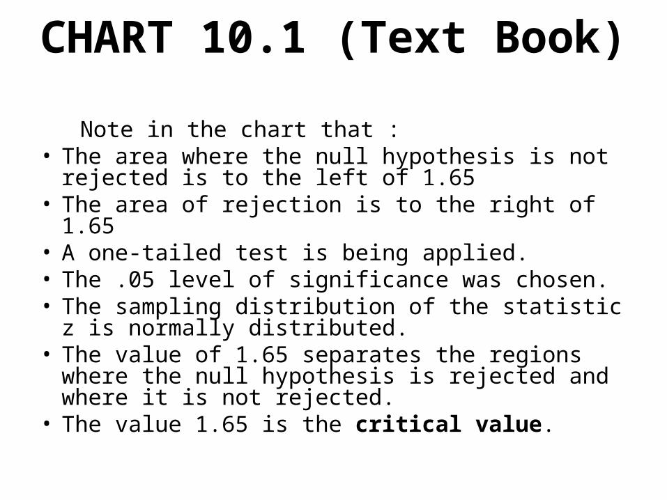
CHART 10.1 (Text Book)

Note in the chart that :• The area where the null hypothesis is not rejected

is to the left of 1.65• The area of rejection is to the right of 1.65• A one-tailed test is being applied.• The .05 level of significance was chosen.• The sampling distribution of the statistic z is

normally distributed.• The value of 1.65 separates the regions where the

null hypothesis is rejected and where it is not rejected.

• The value 1.65 is the critical value.

• CRITICAL VALUE: The dividing point between the region where the null hypothesis is rejected and the region where it is not rejected.

• Step 5: Make a DecisionThe fifth and final step in hypothesis testing is

computing the test statistic, comparing it to the critical value, and making a decision to reject or not to reject the null hypothesis.

• ONE-TAILED AND TWO-TAILED TESTS OF SIGNIFICANCE

• Chart 10.2 (Text Book)• One way to determine the location of the

rejection region is to look at the direction in which the inequality sign in the alternate hypothesis is pointing

• ( either < or > ). For example, test is one-tailed if H1 states > or < .

• In summary, a test is one-tailed when the alternate hypothesis H1 states a direction, such as :

• H0: The mean income of Managers of Computer Companies is $50,000 per year

• H1: The mean income of Managers of Computer Companies is greater than $50,000 per year

• That is,

• H0: =50000• H1: >50000• If no direction is specified in the alternate

hypothesis, we use a two-tailed test. Changing the previous example,

• H0: The mean income of Managers of Computer Companies is $50,000 per year

• H1: The mean income of Managers of Computer Companies is not equal to $50,000 per year.

• That is,

• H0: = 50000• H1: 50000• If the null hypothesis is rejected and H1

accepted in the two-tailed test, the mean income could be significantly greater than $50,000 per year or it could be significantly less than $50,000 per year. To accommodate these two possibilities, the 5 percent area of rejection is divided into the two tails of the sampling distribution

• (2.5 percent each).• Chart 10.3 (Text Book)

• Note that the total area in the normal distribution is 1.0000, found by .9500+.0250+.0250.

TESTING FOR POPULATION MEAN WITH A KNOWN POPULATION STANDARD

DEVIATION [A Two - Tailed Test]

• Example: The weekly production of steel desks of a Company is normally distributed, with a mean of 200 and a standard deviation of 16. Recently, due to market expansion, new production methods have been introduced and new employees hired. The vice president of manufacturing would like to investigate whether there has been a change in the weekly production of the desk. To put it another way, is the mean number of desks produced at the Company different from 200 at the .01 significance level? A sample of 50 was taken and mean was found to be 203.5.

TESTING FOR A POPULATION MEAN:

SMALL SAMPLE • POPULATION STANDARD DEVIATION

UNKNOWN• When the sample size is less than 30 (n<30)

and the population standard deviation is not known, we replace the standard normal distribution with the t distribution.

• To conduct a test of hypothesis using the t distribution, we use the following formula:

ns

Xt

/

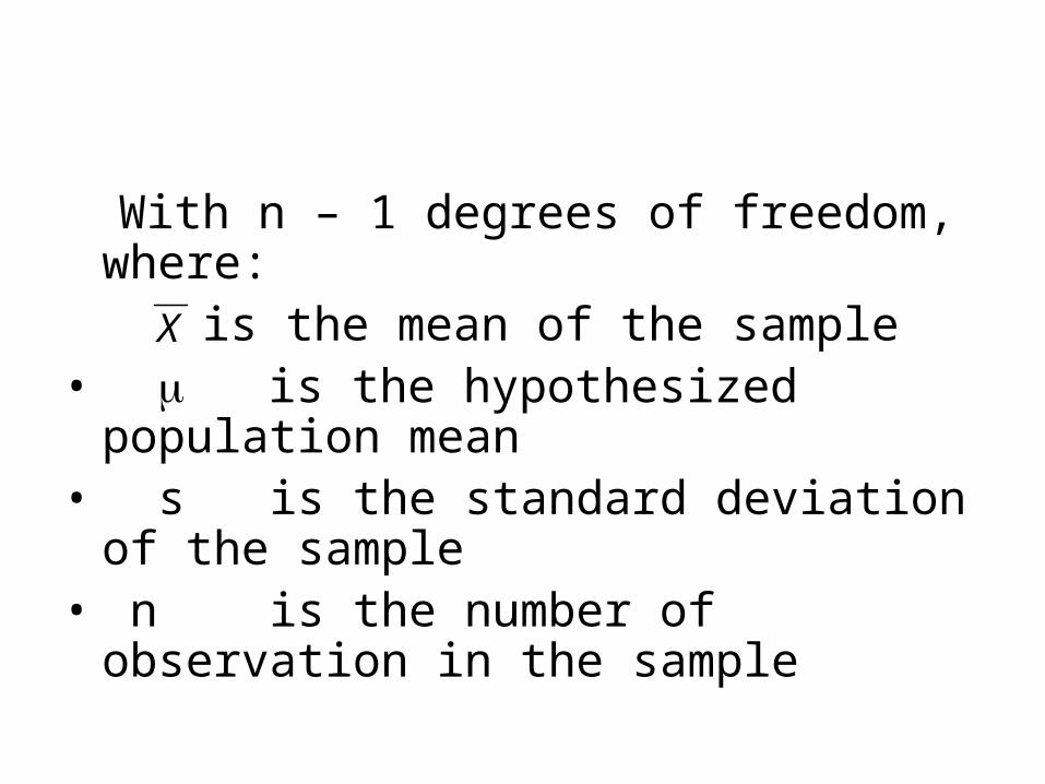
With n – 1 degrees of freedom, where: is the mean of the sample• is the hypothesized population mean• s is the standard deviation of the

sample• n is the number of observation in the

sample

X

EXAMPLE:

• An Insurance Company reports that the mean cost to process a claim is $60. A comparison showed this amount to be larger than most other insurance companies, so they instituted cost-cutting measures.The Insurance Company selected a random sample of 26 recent claims. The mean cost per claim was $57 and the standard deviation was $10. Can they conclude that the cost-cutting measures were effective? Or should they conclude that the difference between the sample mean ($57) and the population mean ($60) is due to chance? Use the .01 significance level. P-value?

SOLUTION: done on the board.

• [Self - Review 10.3 Page: 354 and example at page 355].

• [Self – Review 10.4 Page 358]

• Exercise 15, 17.

TESTS CONCERNING PROPORTIONS

• A proportion is the ratio of the number of successes to the number of observations. We let X refer to the number of successes and n the number of observations, so the proportion of success in a fixed number of trials is X/n. Thus, the formula for computing a sample proportion, p, is p = X/n.

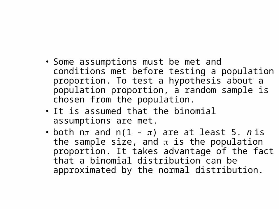
• Some assumptions must be met and conditions met before testing a population proportion. To test a hypothesis about a population proportion, a random sample is chosen from the population.

• It is assumed that the binomial assumptions are met.

• both n and n(1 - ) are at least 5. n is the sample size, and is the population proportion. It takes advantage of the fact that a binomial distribution can be approximated by the normal distribution.

EXAMPLE

• Tina Dennis is the comptroller for Meek Industries. She believes that the current cash-flow problem at Meek is due to the slow collection of accounts receivable. She believes that more than 60 percent of the accounts are in arrears more than three months. A random sample of 200 accounts showed that 140 were more than three months old. At the .01 significance level, can she conclude that more than 60 percent of the accounts are in arrears for more than three months?

Example:

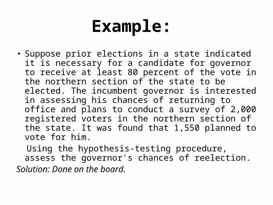
• Suppose prior elections in a state indicated it is necessary for a candidate for governor to receive at least 80 percent of the vote in the northern section of the state to be elected. The incumbent governor is interested in assessing his chances of returning to office and plans to conduct a survey of 2,000 registered voters in the northern section of the state. It was found that 1,550 planned to vote for him.

Using the hypothesis-testing procedure, assess the governor's chances of reelection.

Solution: Done on the board.

p- value in hypothesis testing

• The p-value provides additional insight into the decision. It gives additional information on the strength of the rejection. That is, how confident are we in rejecting the null hypothesis? The p-value compares with the significance level. If the p-value is smaller than the significance level, H0 is rejected. If it is larger than the significance level, H0 is not rejected.

• Determining the p-value not only results in a decision regarding H0 but it gives us additional insight into the strength of the decision. A very small p-value, such as .0001, indicates that there is little likelihood the H0 is true. On the other hand a p-value of .2033 means that H0 is not rejected, and there is little likelihood that it is false.

• How do we compute the p-value? [BOARD].

Two - Sample Tests of Hypothesis

• HYPOTHESIS TESTING: POPULATION MEANS• [Till now we have conducted tests of hypothesis in which we

compared the results of a single sample to a population value. That is, we selected a single random sample from a population and conducted a test of whether the proposed population value was reasonable. We compared the results of a single sample statistic to a population parameter. In this chapter, we expand the idea of hypothesis testing to two samples. That is we select two random samples to determine whether the samples are from the same or equal populations.

• For example, we may want to test: Is there an increase in the production rate if music is piped into the production area?]

EXAMPLE

• Customers at FoodTown super Markets have a choice when paying for their groceries. They may check out and pay using the standard cashier assisted checkout, or they may use the new U-Scan procedure. In the standard procedure a FoodTown employee scans each item, puts it on a short conveyor where another employee puts it in a bag and then into the grocery cart. In the U-Scan procedure the customer scans each item, bags it, and places in the cart themselves.The U-Scan procedure is designed to reduce the time a customer spends in the checkout time.

• The U-Scan facility was recently installed at the Tom Road town location. The store manager would like to know if the mean checkout time using the standard checkout method is longer than the U-Scan. She gathered the following sample information. The time is measured from when the customer enters the line until their bags are in the cart. Hence the time include both waiting in line and checking out. What is the p-value?

Example:

• There have been complaints that resident physicians and nurses on the surgical wing respond too slowly to calls of senior citizens. In fact it is claimed that the other patients receive faster services. Quality assurance department wanted to investigate the allegation. After studying the problem, the department collected the following sample information. At the .01 significance level, is it reasonable to conclude the mean response time is longer for the senior citizen cases? What is the p-value in this case?

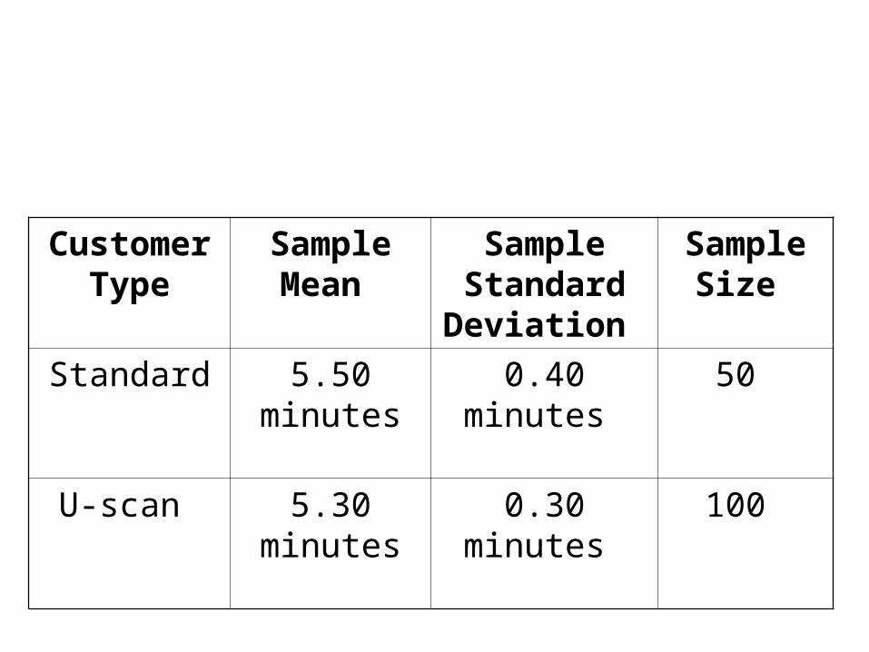
Customer Type

Sample Mean

Sample Standard Deviation

Sample Size

Standard 5.50 minutes

0.40 minutes 50

U-scan 5.30 minutes

0.30 minutes 100

Solution: Done on the board.

• [ Self Review 11-1, page: 383. Exercise 1]

• Go to slide 44 for small samples.

Two sample Tests about proportions• Assumptions are the same as one sample test.Example: Keya Cosmetics recently developed a

new fragrance that they plan to market under the name “Heavenly” . A number of market studies indicate that Heavenly has very good market potential. The sales department is particularly interested in whether there is a difference in the proportions of younger and older women who would purchase Heavenly if it were marketed. There are two independent populations, a population consisting of the younger women and a population consisting of the older women.Each sampled woman will be asked to smell Heavenly and indicate whether she likes the fragrance well enough to purchase a bottle.

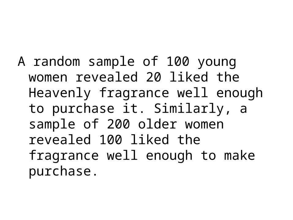
A random sample of 100 young women revealed 20 liked the Heavenly fragrance well enough to purchase it. Similarly, a sample of 200 older women revealed 100 liked the fragrance well enough to make purchase.

DEPENDENT SAMPLES

• In our previous example, we tested the difference between the means from two independent samples. This means, for example,

that the sample response time for the senior citizens is unrelated to the response time for the other patients. If Mr. Rahman is a senior citizen and his response time is sampled, that does not affect the response time for any other patient.

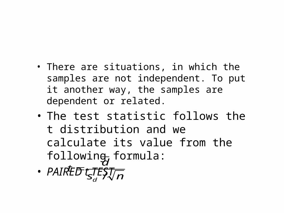
• There are situations, in which the samples are not independent. To put it another way, the samples are dependent or related.

• The test statistic follows the t distribution and we calculate its value from the following formula:

• PAIRED t TEST

ns

dt

d /

• There are n-1 degrees of freedom and

dis the mean of the difference between the paired or related observations

ds

is the standard deviation of the differences between the paired or related observations.

• n is the number of paired observations.

Example:

• A loan giving organization wishes to compare the two companies they use to appraise the value of residential homes. The Organization selected a sample of 10 residential properties and scheduled both firms for an appraisal. The results, reported in $000, are:

Home 1 2 3 4 5 6 7 8 9 10

Co. A 135 110 131 142 105 130 131 110 125 149

Co. B 128 105 119 140 98 123 127 115 122 145

Home Co. A Co. B Difference, d d2

1 135 128 7 49

2 110 105 5 25

3 131 119 12 144

4 142 140 2 4

5 105 98 7 49

6 130 123 7 49

7 131 127 4 16

8 110 115 -5 25

9 125 122 3 9

10 149 145 4 16

Total 46 386

• At the .05 significance level, can we conclude there is a difference in the mean appraised values of the homes?

• SOLUTION: Done on the board.• To find the p-value, we use Appendix F and the

section for a two-tailed test. Move along the row with 9 degrees of freedom and find the values of t that are closest to our calculated value. For a .01 significance level, the value of t is 3.250. The computed value is larger than this value, but smaller than the value of 4.781 corresponding to the .001 significance level. Hence, the p-value is less than .01.

Comparing Populations with Small

Samples

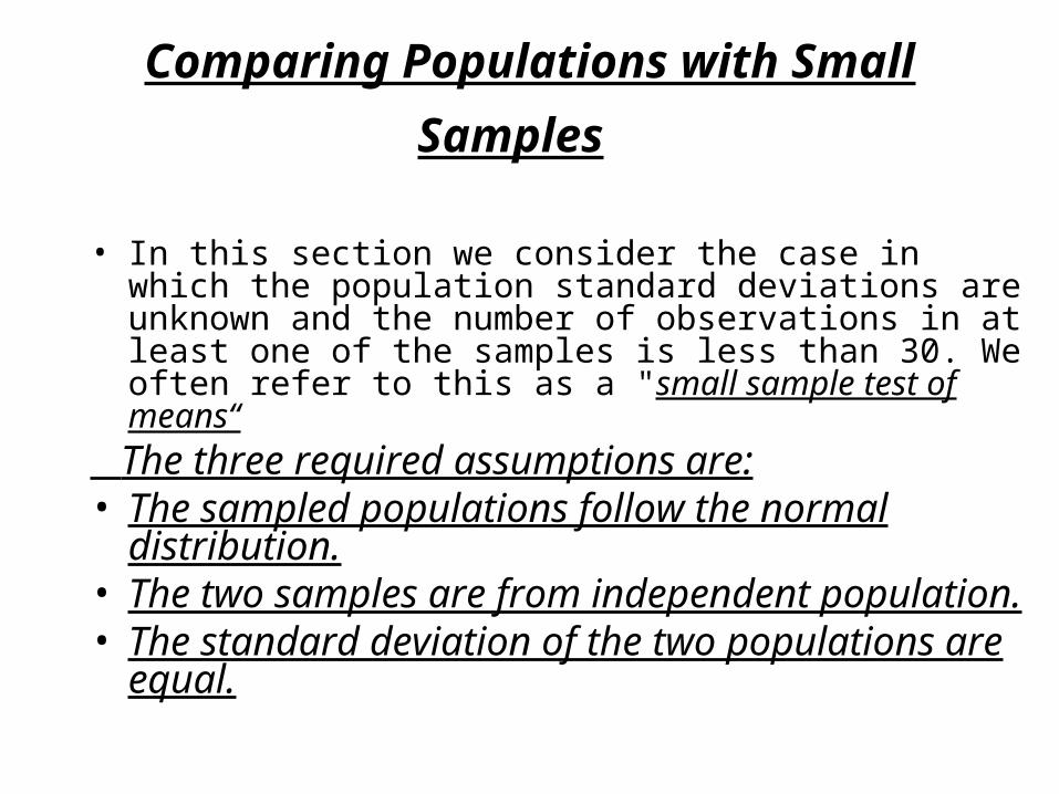
• In this section we consider the case in which the population standard deviations are unknown and the number of observations in at least one of the samples is less than 30. We often refer to this as a "small sample test of means“

The three required assumptions are:• The sampled populations follow the normal

distribution.• The two samples are from independent

population.• The standard deviation of the two populations

are equal.

• The test statistic is the t distribution.

• The following formula is used to pool the sample variances. Notice that two factors are involved: the number of observations in each sample and the sample standard deviations themselves.

• Pooled Variance :

S2p=

2

)1()1(

21

222

211

nn

snsn

Where:

• s12 is the variance (standard deviation

squared) of the first sample.

• s22 is the variance of the second sample.

• The value of t is computed from the following equation:

)11

(21

2

21

nns

XXt

p

• Where: • is the mean of the first sample.• is the mean of the second sample.• is the number of observations in first

sample.• is the number of observations in

second sample.• is the pooled estimate of the

population variance.

1X2X

1n

2n2ps

2ps

• The number of degrees of freedom in the test is the total number of items sampled minus the total number of samples. Because there are two samples, there are n1 + n2 - 2 degrees of freedom.

Example:

• The production manager, at a manufacturer of wheelchairs, wants to compare the number of defective wheelchairs produced on the day shift with the number on the afternoon shift. A sample of the production from 6 day shifts and 8 afternoon shifts revealed the following number of defects.

Day 5 8 7 6 9 7

Afternoon 8 10 7 11 9 12 14 9

At the .05 significant level, is there a difference in the mean number of defects per shift?

What is the p-value?

Interpret the result.

Solution: Done on the board.

TEST CONCERING PROPORTION