hysdel 3.0 – manual - eth zpeople.ee.ethz.ch/~cohysys/hysdel/download/hysdel3_manual.pdf · •...
TRANSCRIPT

HYSDEL 3.0 – Manual

Institute of Information Engineering, Automation, and MathematicsSlovak University of Technology in BratislavaRadlinskeho 9812 37 BratislavaSLOVAKIA
Martin Herceg, [email protected]
Michal Kvasnica, [email protected] (corresponding author)
Eidgenossische Technische Hochschule ZurichAutomatic Control LaboratoryETL I 28Physikstrasse 38092 ZurichSWITZERLAND
Manfred Morari, [email protected]
ABB Switzerland LtdCorporate ResearchSegelhofstrasse 1CH-5405 Baden-DattwilSWITZERLAND
Sebastian Gaulocher, [email protected]
Jan Poland, [email protected]
ii

Contents
1 Introduction 1
1.1 HYSDEL . . . . . . . . . . . . . . . . . . . . . . . . . . . . . . . . . . . . . . 11.2 Motivation . . . . . . . . . . . . . . . . . . . . . . . . . . . . . . . . . . . . . 11.3 Goals and Deliverables . . . . . . . . . . . . . . . . . . . . . . . . . . . . . . . 2
2 Installation 3
2.1 Installation of HYSDEL 3.0 . . . . . . . . . . . . . . . . . . . . . . . . . . . . 3
3 Modeling of hybrid systems 4
3.1 Mixed-Logical Dynamic System Description . . . . . . . . . . . . . . . . . . . 43.1.1 HYSDEL 2.0.5 MLD system formulation . . . . . . . . . . . . . . . . . 43.1.2 HYSDEL 3.0 MLD system formulation . . . . . . . . . . . . . . . . . . 4
4 Using HYSDEL 3.0 6
4.1 Implementation of HYSDEL 3.0 . . . . . . . . . . . . . . . . . . . . . . . . . 64.2 Quick Start . . . . . . . . . . . . . . . . . . . . . . . . . . . . . . . . . . . . . 74.3 Model optimization . . . . . . . . . . . . . . . . . . . . . . . . . . . . . . . . . 94.4 Simulations with HYSDEL 3.0 . . . . . . . . . . . . . . . . . . . . . . . . . . 10
5 HYSDEL 3.0 - Language Description 13
5.1 Preliminaries . . . . . . . . . . . . . . . . . . . . . . . . . . . . . . . . . . . . 135.2 List of Language Changes . . . . . . . . . . . . . . . . . . . . . . . . . . . . . 145.3 INTERFACE Section . . . . . . . . . . . . . . . . . . . . . . . . . . . . . . . . 14
5.3.1 INPUT section . . . . . . . . . . . . . . . . . . . . . . . . . . . . . . . 155.3.2 STATE section . . . . . . . . . . . . . . . . . . . . . . . . . . . . . . . 175.3.3 OUTPUT section . . . . . . . . . . . . . . . . . . . . . . . . . . . . . . 195.3.4 PARAMETER section . . . . . . . . . . . . . . . . . . . . . . . . . . . 205.3.5 MODULE section . . . . . . . . . . . . . . . . . . . . . . . . . . . . . 22
5.4 IMPLEMENTATION Section . . . . . . . . . . . . . . . . . . . . . . . . . . . 245.4.1 Indexing . . . . . . . . . . . . . . . . . . . . . . . . . . . . . . . . . . . 255.4.2 FOR loops . . . . . . . . . . . . . . . . . . . . . . . . . . . . . . . . . 275.4.3 HYSDEL operators and built-in functions . . . . . . . . . . . . . . . . 295.4.4 Casting Boolean to real . . . . . . . . . . . . . . . . . . . . . . . . . . 305.4.5 AUX section . . . . . . . . . . . . . . . . . . . . . . . . . . . . . . . . 305.4.6 CONTINUOUS section . . . . . . . . . . . . . . . . . . . . . . . . . . 325.4.7 AUTOMATA section . . . . . . . . . . . . . . . . . . . . . . . . . . . . 325.4.8 LINEAR section . . . . . . . . . . . . . . . . . . . . . . . . . . . . . . 335.4.9 LOGIC section . . . . . . . . . . . . . . . . . . . . . . . . . . . . . . . 345.4.10 AD section . . . . . . . . . . . . . . . . . . . . . . . . . . . . . . . . . 345.4.11 DA section . . . . . . . . . . . . . . . . . . . . . . . . . . . . . . . . . 355.4.12 MUST section . . . . . . . . . . . . . . . . . . . . . . . . . . . . . . . 365.4.13 OUTPUT section . . . . . . . . . . . . . . . . . . . . . . . . . . . . . . 38
iii

5.5 Merging of HYSDEL Files . . . . . . . . . . . . . . . . . . . . . . . . . . . . . 385.5.1 Creating slave files . . . . . . . . . . . . . . . . . . . . . . . . . . . . . 385.5.2 Creating master files . . . . . . . . . . . . . . . . . . . . . . . . . . . . 415.5.3 Automatic generation of master files . . . . . . . . . . . . . . . . . . . 42
5.6 EXAMPLES . . . . . . . . . . . . . . . . . . . . . . . . . . . . . . . . . . . . 455.6.1 Simple code . . . . . . . . . . . . . . . . . . . . . . . . . . . . . . . . . 455.6.2 Vectorized code . . . . . . . . . . . . . . . . . . . . . . . . . . . . . . . 475.6.3 Advanced code . . . . . . . . . . . . . . . . . . . . . . . . . . . . . . . 49
6 Control design with HYSDEL 3.0 52
6.1 Export of MLD system to PWA model . . . . . . . . . . . . . . . . . . . . . . 52
iv

1 Introduction
1.1 HYSDEL
HYSDEL (HYbrid SYstem DEscription Language) [8, 9] is a high-level modeling languagefor the specification of hybrid systems representable by discrete hybrid automata (DHA). Itallows hybrid models to be formulated in a manner appealing to the application engineer.The description of a hybrid system in HYSDEL is on an abstract, descriptive level. A toolcalled HYSDEL compiler uses the abstract HYSDEL description to generate computationalmodels in the form of mixed-logic dynamical (MLD) or piecewise-affine (PWA) systems,that can then be used in computations related to system optimization, verification or controlsynthesis.Unlike general-purpose optimization modeling languages (e.g. AMPL or GAMS), HYS-
DEL is a specialized language for describing a continuous dynamic behavior combined withlogical conditions. Tailored to the specific class of problems, algorithms implemented inthe HYSDEL compiler generate models which are more compact and which render the op-timization problems using such models more efficient compared to formulations obtainedby general-purpose modeling software (e.g. AMPL). Posing an optimization problem us-ing general-purpose languages may become a tedious task when it comes to cases involvingdynamic behavior.
1.2 Motivation
Since its inception 4 years ago until the current version 2.0.5, HYSDEL has gone through anumber of changes. However, during the last 2 years the development of HYSDEL has notbeen following the progress of research in the topic. In particular, the generation of MLDmodels from logic conditions uses a relatively limited set of algorithms originally imple-mented in HYSDEL compiler, while recently several tools have emerged providing means formore advanced MLD and PWA model formulations, most notably Multi-Parametric Toolbox(MPT).From the usability point of view, the current version of HYSDEL as a language has some
major drawbacks. In particular, it does not support vectors and matrices as variables andlacks important language constructs like loops. These drawbacks make the description oflarge models cumbersome and prone to errors.The main obstacle for maintenance and improvement of HYSDEL is the fact that the
C++ implementation of the compiler, containing ca 10000 lines of code, is poorly docu-mented and the code is written according to obsolete standards of the C++ language. Anymajor extension of the language and the compiler requires high familiarity with the sourcecode. Having in mind relatively frequent changes in the personnel responsible for HYSDELmaintenance, this requirement cannot be easily met and concerns related to issue have beenrepeatedly expressed by Andreas Poncet and Eduardo Gallestey.
1

HYSDEL 3.0 1 Introduction
1.3 Goals and Deliverables
The planned modifications of HYSDEL are summarized in the following:
• Rewriting the HYSDEL parser in MATLAB. This change would dramatically increasethe maintainability of HYSDEL. More importantly, it would make the integration withother tools available in MATLAB tighter. In particular, it would be possible to useoptimization tools and to prune an MLD/PWA model during its generation. An idealcomputational engine for such a task would be YALMIP. The expected outcome fromthis change is a significant improvement in compactness of the generated models thatwould also result in an increased efficiency of the optimization procedure using themodels. It should be stressed that the way how the optimization model is formulatedmay be crucial for the solvability of the optimization problem.
• Extending basic HYSDEL syntax. This change would address extension of the HYS-DEL to support variable constructs like vectors and matrices. A Matlab implementa-tion of the HYSDEL parser makes this extension straightforward. The syntax would befurther expanded to include paradigms like (nested) loops and to improve the syntaxof IF-THEN-ELSE blocks.
• Increase modularity. When defining large models, it is convenient to impose a modulardesign paradigm by introducing compositional models that comprise several HYSDELfiles interconnected through common continuous/discrete variables. This modificationwould essentially be done on a syntactical level. It should ensure, for example thatthe optimization problems are not unnecessarily bloated when parts of the model areswitched off in certain modes.
• Merging of Models. Related to the modularity issue, the ETH should investigate theexisting method developed by ABB to merge MLD models, and evaluate whetherthere are better alternatives, with respect to the size and compactness of the resultingmodels. The results of this investigation are to be kept confidential at the discretionof ABB.
In its current business, ABB relies on having a non-MATLAB based compiler that can beused, for example, on site by untrained personnel and without the requiirement of additionallicenses. As such the ETH is to investigate concepts that will enable use of the developedplatform without a MATLAB license, e.g. based on the MATLAB Compiler.
2
2 Installation
2.1 Installation of HYSDEL 3.0
Prerequisites to use HYSDEL 3.0 is to have MATLAB installed, with version newer as 7.0.Secondly, for proper use of all functions, it is desirable to have following toolboxes installed:
• MATLAB Simulink (for graphical modeling)
• YALMIP [7] (for compilation of HYSDEL files)http://control.ee.ethz.ch/~joloef/wiki/pmwiki.php
• MPT Toolbox [5] (for visualization, MLD model tweaking, desing of predictive control)http://control.ee.ethz.ch/~mpt/
YALMIP and MPT Toolboxes are available at the aforementioned web addresses under theGPL public license. HYSDEL 3.0 can be downloaded at the following link
http://autlux03.ee.ethz.ch:8000/hysdel3/wiki.
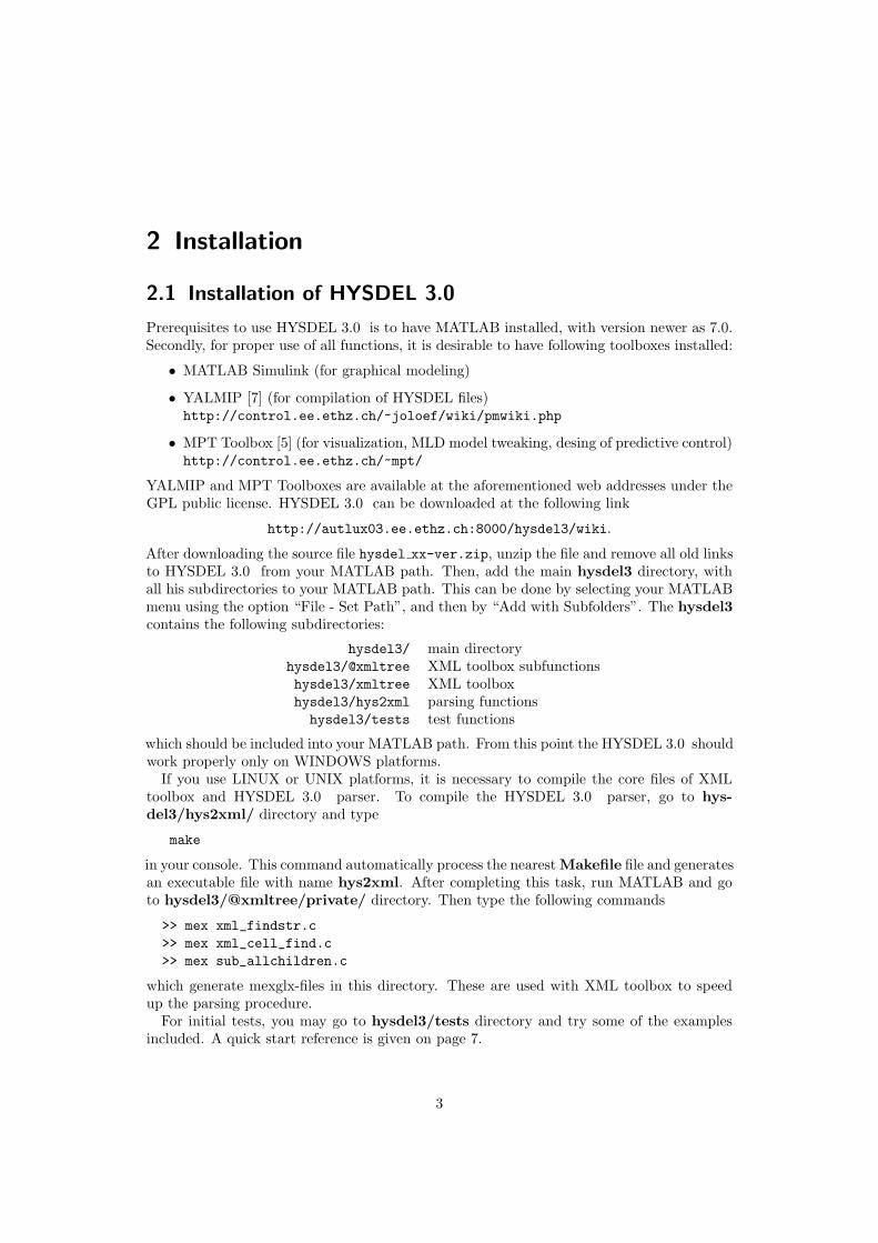
After downloading the source file hysdel xx-ver.zip, unzip the file and remove all old linksto HYSDEL 3.0 from your MATLAB path. Then, add the main hysdel3 directory, withall his subdirectories to your MATLAB path. This can be done by selecting your MATLABmenu using the option “File - Set Path”, and then by “Add with Subfolders”. The hysdel3contains the following subdirectories:
hysdel3/ main directoryhysdel3/@xmltree XML toolbox subfunctionshysdel3/xmltree XML toolboxhysdel3/hys2xml parsing functionshysdel3/tests test functions
which should be included into your MATLAB path. From this point the HYSDEL 3.0 shouldwork properly only on WINDOWS platforms.If you use LINUX or UNIX platforms, it is necessary to compile the core files of XML
toolbox and HYSDEL 3.0 parser. To compile the HYSDEL 3.0 parser, go to hys-del3/hys2xml/ directory and type
make
in your console. This command automatically process the nearestMakefile file and generatesan executable file with name hys2xml. After completing this task, run MATLAB and goto hysdel3/@xmltree/private/ directory. Then type the following commands
>> mex xml_findstr.c
>> mex xml_cell_find.c
>> mex sub_allchildren.c
which generate mexglx-files in this directory. These are used with XML toolbox to speedup the parsing procedure.For initial tests, you may go to hysdel3/tests directory and try some of the examples
included. A quick start reference is given on page 7.
3

3 Modeling of hybrid systems
3.1 Mixed-Logical Dynamic System Description
Mixed Logical Dynamical (MLD) systems describe in general the behavior of linear discrete-time systems with integrated logical rules. The basic principles, how logical rules are in-corporated into overall MLD description, and the theory fundamentals are explained in [2].This publication is a main source for further references regarding the modeling and controlof hybrid systems.
3.1.1 HYSDEL 2.0.5 MLD system formulation
HYSDEL 2.0.5 considers the MLD description, as given in [2], as fundamental for modelingof hybrid systems. In this MLD formulation, the evolution of a hybrid system is given by aset of following equations
x(k + 1) = Ax(k) +B1u(k) +B2δ(k) +B3z(k) (3.1a)
y(k) = Cx(k) +D1u(k) +D2w(k) +D3z(k) (3.1b)
E2δ(k) + E3z(k) ≤ E1u(k) + E4x(k) + E5 (3.1c)
where (3.1a) is the state-update equation, (3.1b) is the output equation, and linear inequal-ities (3.1c) describe the switching conditions between the hybrid modes. The MLD model(3.1) uses standard notations, i.e. x ∈ R
nxr × {0, 1}nxb is a vector of continuous and binarystates, u ∈ R
nur × {0, 1}nub are the (cont. and binary) inputs, y ∈ Rnyr × {0, 1}nyb vector
of (cont. and binary) outputs, δ ∈ {0, 1}nd represent auxiliary binary, z ∈ Rnz continuous
variables, respectively, and A, B1, B2, B3, C, D1, D2, D3, E2, E3, E1, E4, E5 are matricesof suitable dimensions. For a given state x(k) and input u(k) the evolution of the MLDsystem (3.1) is determined by solving δ(k) and z(k) from (3.1c) and updating x(k+1), y(k).
However, due to the extensive use of HYSDEL 2.0.5, the interpretation of MLD sys-tem (3.1) was sometimes misleading when formulating control problems and several short-comings have been identified. More precisely, the form (3.1c) does not explicitly coverequality constraints as they have to be formulated as double-sided inequalities. Secondly,binary and real variables are not treated equally in the formulation, i.e. sometimes theyare part of one vector (x, u, y), and sometimes they are separated (d, z). Furthermore, theMLD description (3.1) does not consider affine terms directly, numerical indexing of ma-trices is misleading, etc. To overcome these shortcomings, the HYSDEL 3.0 uses differentformulation of MLD system (3.1) which will be explained in the next section.
3.1.2 HYSDEL 3.0 MLD system formulation
Arising from numerous shortcomings of the MLD model used by HYSDEL 2.0.5, the HYS-DEL 3.0 uses more flexible form to describe the behavior of hybrid systems. In orderto clearly distinguish between binary/continuous variables and equalities/inequalities in theMLD formulation, sets of indices are added to the MLD form and new notations are adopted.
4

HYSDEL 3.0 3 Modeling of hybrid systems
More precisely, the new MLD description is given by
x(k + 1) = Ax(k) +Buu(k) +Bauxw(k) +Baff (3.2a)
y(k) = Cx(k) +Duu(k) +Dauxw(k) +Daff (3.2b)
Exx(k) + Euu(k) + Eauxw(k) ≤ Eaff (3.2c)
{sets of indices} Jx, Ju, Jw, Jeq, Jineq (3.2d)
where the auxiliary vector w(k) comprises of two elements w(k) = [z(k), δ(k)]T . Comparingto the previous description (3.1), these changes are visible
• Matrices B1, D1, and E1 are referred to as Bu, Du, and Eu, respectively.
• Auxiliary variables δ(k) and z(k) are merged together in one vector 1 called w(k) =[z(k), δ(k)]T
• Matrix couples B3 - B2, D3 - D2, E3 - E2 are referred to as Baux = [B3 B2], Daux =[D3 D2], Eaux = [E3 E2], respectively.
• Affine terms Baff , Daff are included.
• E4 and E5 are now referred to as Ex and Eaff , respectively. Moreover, the set ofinequalities in (3.1) is rewritten to a condensed form (3.2c) and their relations to theold form are Ex = −E4 and Eu = −E1.
• Indices (3.2d) indicate which variables in the vector correspond to real/binary forstates Jx, inputs Ju, and auxiliaries Jw. Additionally, Jeq corresponds to a set ofindices which define rows of matrices (3.2c) with equality constraints and Jineq withinequalities, i.e.
Eeqx x(k) + Eeq
u u(k) + Eeqauxw(k) = Eeq
aff
Eineqx x(k) + Eineq
u u(k) + Eineqaux w(k) ≤ Eineq
aff
Structure of the indexed sets Jx, Ju, Jw is vector-wise and it distinguishes between binaryand real variables with strings ’r’, ’b’. Precisely, string ’r’ refers to real and string ’b’ refersto Boolean variable, e.g.
{Jx, Ju, Jw} =
’r’
’r’
’b’
’r’
corresponds to
REAL
REAL
BOOL
REAL
To be able to determine the position of a given real/binary variable in a vector, these setscontain also a numerical information. For instance, the location of equality constraints inmatrices (3.2c) is given by Jeq and refers to rows in (3.2c) which form equalities e.g.
Jeq =
158
corresponds to
1st row is an equality constraint5th row is an equality constraint8th row is an equality constraint
Next section describes how the HYSDEL 3.0 generates the MLD model (3.2) and how theobtain all of the data stored in the MLD structure (3.2).
1Positions of real/binary variables in this vector can be in different order, this is specified by indexed setJw.
5

4 Using HYSDEL 3.0
4.1 Implementation of HYSDEL 3.0
Implementation of the HYSDEL 3.0 does not differ from the procedure in HYSDEL 2.0.5.The process of generating the MLD model (3.2) starts with writing the HYSDEL source fileusing the HYSDEL language. Consequently, this file is compiled to an appropriate format,which is processed by MATLAB and the output is the MLD structure. This procedure issketched in Fig. 4.1.
Figure 4.1: Generation of MLD model comprises of compilation of the HYSDEL file and generation
of file acceptable by MATLAB.
HYSDEL 2.0.5 uses compiler written in C++ language, which has its own advantages anddisadvantages. Crucial part is, that in HYSDEL 3.0 the compilation is totally replaced bya YALMIP module. “YALMIP is a modeling language for defining and solving advancedoptimization problems. It is implemented as a free toolbox for MATLAB” [6]. There areseveral reasons for including YALMIP package [7] into HYSDEL 3.0 version, namely
• easier maintainability of the compiler
• faster compilation
• direct handling of advanced syntax
• improved condition checking and merging features
• automatic model optimization.
Figure 4.2: New path of generating executable MLD models relies on YALMIP package.
Since YALMIP is a toolbox for MATLAB, manipulation with HYSDEL 3.0 requiresknowledge of standard elementary operations with MATLAB, e.g. declaration of variables,accessing internal variable data, concatenating, indexing etc. Furthermore, HYSDEL 3.0has borrowed MATLAB syntax and thus it is advisable for user to obtain a basic experiencewith MATLAB.
6
HYSDEL 3.0 4 Using HYSDEL 3.0
4.2 Quick Start
Procedure for generation of the MLD system (3.2) starts in writing a corresponding HYSDELfile in your favorite editor using the HYSDEL language and specifying the suffix .hys.Assume, that a file with name my file.hys was created and written in HYSDEL language.To get an appropriate MLD representation, the file needs to be compiled in MATLABenvironment. HYSDEL 3.0 uses the same syntax as an old version of HYSDEL used to do,i.e.
>> hysdel3(’my file.hys’)
where hysdel3 is the main routine for processing the compilation. The routine accepts thepath for HYSDEL file which can be written is several forms:
• hysdel3(’my file’), without specifying the file suffix
• hysdel3(’dir/subdir/my file’), with path including subdirecories
• hysdel3(’../my file’), with path referring to higher direcory etc.
By invoking this command in MATLAB, an m-file equivalent of the my file.hys, i.e.my file.m is generated in the current directory. This new generated m-file is basicallya YALMIP code which contains whole information given by my file.hys. Depending onthe structure of the HYSDEL file, the m-file my file.m serves as a function for generatingthe MLD representation. If the original HYSDEL file does not contain any symbolic vari-ables, the MLD structure can be obtained by typing simply the same name
>> my file
Otherwise, if some symbolic variables are declared in the original hys-file, it is necessary toassign particular values to these variables before calling the my file function. For instance,if the hys-file contains two symbolic parameters a, b, we create a structure with concretevalues, e.g.
>> params.a = 1;
>> params.b = -0.3;
Consequently, the MLD structure can be obtained by including the structure params as anargument, i.e.
>> my file(params)
For backwards compatibility, the generated function returns also an old MLD form (3.1).This can be achieved by
>> [S, Sold] = my file(params).
where the new MLD structure is returned in variable S and old MLD structure in variableSold.When the structure S with MLD description is available, each particular information about
the MLD model (3.2) can be extracted using the MATLAB “dot” syntax. HYSDEL 3.0 usesthe same notations as HYSDEL 2.0.5, e.g. dimensions of the variables have the followingnotations
S.nx /* dimension of states */
.nxr /* dimension of real states */
.nxb /* dimension of binary states */
7

HYSDEL 3.0 4 Using HYSDEL 3.0
.nu /* dimension of inputs */
.nur /* dimension of real inputs */
.nub /* dimension of binary inputs */
.ny /* dimension of outputs */
.nyr /* dimension of real outputs */
.nyb /* dimension of binary outputs */
.nw /* dimension of auxiliary variables */
.nz /* dimension of auxiliary real variables */
.nd /* dimension of auxiliary binary variables */
.nc /* dimension of constraints (equalities + inequalities) */
Matrices introduced in MLD model (3.2) are stored as fields with the same name, i.e.
S.A
.Bu
.Baux
.Baff
.C
.Du
.Daux
.Daff
.Ex
.Eu
.Eaux
.Eaff
and indexed sets are accessible through substructure J
S.J.X /* string of indices (’r’ or ’b’) for states */
.J.U /* string of indices (’r’ or ’b’) for inputs */
.J.Y /* string of indices (’r’ or ’b’) for outputs */
.J.W /* string of indices (’r’ or ’b’) for auxiliary variables */
Information about the numerical position of variables in a vector is given by a substructurej, i.e.
S.j.xr /* indices of REAL states */
.j.xb /* indices of BOOL states */
.j.ur /* indices of REAL inputs */
.j.ub /* indices of BOOL inputs */
.j.yr /* indices of REAL outputs */
.j.yb /* indices of BOOL outputs */
.j.d /* indices of BOOL auxiliary variables */
.j.z /* indices of REAL auxiliary variables /*
.j.eq /* indices of equality constraints */
.j.ineq /* indices of inequality constraints */
Further information about the MLD model are stored in remaining substructures of thevariable S. Here belong the names, types, and dimensions of declared variables, i.e.
S.InputName /* names of input variables */
.InputKind /* types of the input variables (real, binary) */
.InputLength /* dimensions of the input variables */
8

HYSDEL 3.0 4 Using HYSDEL 3.0
.StateName /* names of state variables */
.StateKind /* types of the state variables (real, binary) */
.StateLength /* dimensions of the state variables */
.OutputName /* names of output variables */
.OutputKind /* types of the output variables (real, binary) */
.OutputLength /* dimensions of the output variables */
.AuxName /* names of auxiliary variables */
.AuxKind /* types of the auxiliary variables (real, binary) */
.AuxLength /* dimensions of the auxiliary variables */
upper and lower bounds
S.xl /* lower bound on state variables */
.xu /* upper bound on state variables */
.ul /* lower bound on input variables */
.uu /* upper bound on input variables */
.wl /* lower bound on auxiliary variables */
.wu /* upper bound on auxiliary variables */
The number of total constraints is given by the field
S.nc /* total number of constraints (equalities + inequalities) */
Information about possible symbolic variables in the HYSDEL file is stored in the field
S.symtable /* information about declared variables */
as a substructure with additional fields. Validity of the resulting MLD model indicates thefield
S.MLDisvalid /* is the MLD model valid */
Since HYSDEL 3.0 offers merging of several MLD structures on a syntactical level, theinformation about the interconnections between the local models is stored in field
S.connections /* table of interconnections between HYSDEL modules */
Detailed explanation of this feature will be available later, in the merging section.
4.3 Model optimization
One of the significant feature, which offers HYSDEL 3.0 , is model optimization. Thepurpose of model optimization is to exploit as much as possible the structure of the providedconstraints, such that the simulation of the resulting MLD system is faster. It has beenstudied in [4] that the quality of the model can be influenced by big-M formulation [2].The big-M notion comes in play when logical relations are mixed with certain constraintsatisfaction and this is the case of DA or AD section. HYSDEL 2.0 allowed to specify thesebounds directly, but HYSDEL 3.0 has this feature disabled and the bounds are computedautomatically.HYSDEL 3.0 offers further model optimization, using the option ’optimize’ when
calling the compiled file as a function. The procedure for generating better quality modelsrequires first compilation of a hys-file, e.g.
>> hysdel3(’my file.hys’)
9

HYSDEL 3.0 4 Using HYSDEL 3.0
and secondly, the model optimization can be invoked using
>> [S, Sold] = my file.hys(’optimize’)
option. If the HYSDEL 3.0 contains any symbolic variables, the use is as follows
>> [S, Sold] = my file.hys(parameters, ’optimize’)
where the structure parameters contains concrete values assigned to symbolic variables.
Note that model optimization is not used by default. This is because this routine requiresa search through sets of defined constraints and it may be time consuming.
4.4 Simulations with HYSDEL 3.0
As long as the MLD structure is available in the MATLAB workspace, it is possible tosimulate the evolution of a hybrid system using the command
>> [xnew, y, w, feas] = h3 mldsim(S, x0, u0)
where
x0 initial state x(k)u0 control input u(k)
xnew state update x(k + 1)y output y(k) associated to x(k) and u(k)w feasible value of the auxiliary variables w(k)
feas 1/0 flag whether the problem was feasible for given x(k) and u(k)
The output contains the successor states x(k+1) for given combination of initial state x(k)and input u(k) for one time step. For multiple time steps, it is required to loop this commandfor changing values of x(k) and u(k).Another option is to use a graphical level of HYSDEL 3.0 . This feature exploits the MAT-
LAB Simulink environment is incorporated as a separate library block. The HYSDEL 3.0Simulink library can be run with help of command
>> h3 lib
and outputs a block called “HYSDEL Model” as shown in Fig. 4.3. The HYSDEL 3.0 blockcontains several fields, namely
path to HYSDEL source filestructure with particular values for symbolic variablessampling time (default value is 1)initial condition x(k)
which are necessary for compilation and simulation of MLD system. Some of these fieldswill be automatically filled with empty brackets “[]” if the hys-file does not contain anysymbolical parameters or no states.After filling the fields in “HYSDEL Model” block, HYSDEL 3.0 automatically compiles
the source file and generates the MLD structure. This block is consequently transformed toa subsystem, which contains the equal number of input/output ports as they were declaredin the hys-file and an S-Function with MLD model. Real and binary ports are colorfullyseparated as this is nicely illustrated in Fig. 4.5. To obtain a time evolution of the MLDsystem it is needed to connect the input/output ports with appropriate data source blocks,
10

HYSDEL 3.0 4 Using HYSDEL 3.0
Figure 4.3: HYSDEL 3.0 contains a Simulink library block “HYSDEL Model”.
Figure 4.4: “HYSDEL Model” block accepts the source HYSDEL file with additional parameters.
as well as with output blocks, which are available in standard Simulink library. An exampleof a simple simulation scenario is also depicted in Fig. 4.5.Note that if Simulink scheme contains several blocks “HYSDELModel”, the time needed to
simulate the scheme increases because Simulink has to solve multiple optimization problemsin one sampling time. Therefore, it is recommended for user to merge multiple MLD systemsinto one large MLD structure and use this large MLD for simulation. The merging featureis new in HYSDEL 3.0 and it is done on a HYSDEL language level.
11

HYSDEL 3.0 4 Using HYSDEL 3.0
Figure 4.5: “HYSDEL Model” block automatically generates input/output ports according to de-
clared inputs/outputs in the HYSDEL source file.
12

5 HYSDEL 3.0 - Language Description
This chapter describes new features available in this version 3.0 of HYSDEL. The aim willbe to outline differences comparing to HYSDEL 2.0.5 version and interpret the new syntaxon simple examples. The structure of this chapter follows the syntactical parts of HYSDELscripting language.
5.1 Preliminaries
A HYSDEL syntax was developed on C-language, and many symbols are thus similar. Struc-turally, a standard HYSDEL file (or hys-file) comprises of two modes, namely INTERFACEand IMPLEMENTATION. Each of the sections is delimited by curly brackets e.g.
section {
...
}
and this holds for every kind of subsections as well. If one wants to add comments, this issimply done via C-like comments, i.e.
section {
...
/* this line is commented */
...
}
An example of the simplest HYSDEL file might look as follows
SYSTEM name {
/* example of HYSDEL file structure */
INTERFACE {
/* interface part serves as declaration of variables */
}
IMPLEMENTATION {
/* implementation part defines relations between declared variables */
}
}
Note that the file begins with SYSTEM string which is followed by the name. The namecan be arbitrary, but it should be kept in mind that it usually points to a real object,therefore is recommended to use labels as e.g. tank, valve, pump, belt, etc. Other stringslike INTERFACE and IMPLEMENTATION are obligatory. HYSDEL file can be createdwithin any preferred text editor, however, the file should always have the suffix “.hys”, e.g.tank.hys. More importantly, it is recommended to use the name of the SYSTEM also asthe file name, e.g. system called tank will be a file tank.hys etc. This becomes reasonableif there are more HYSDEL files in one directory and helps to identify the files easily. In thenext content, the aim is to interpret new syntactical changes comparing to HYSDEL 2.0.5version.
13
HYSDEL 3.0 5 HYSDEL 3.0 - Language Description
5.2 List of Language Changes
The list of topics of syntactical changes in HYSDEL 3.0 is briefly summarized in the sequel,while the details will be explained in particular sections.
• INTERFACE section
– extensions of the INTERFACE section
– declaration of INPUT, STATE, OUTPUT variables in scalar/vectorized form
– declaration of parameters
– declaration of subsystems
• IMPLEMENTATION section
– extensions of the IMPLEMENTATION section
– indexing
– FOR and nested FOR loops
– operators and built-in functions
– AUX section
– CONTINUOUS section
– AUTOMATA section
– LINEAR section
– LOGIC section
– AD section
– DA section
– MUST section
– OUTPUT section
• Merging of HYSDEL files
5.3 INTERFACE Section
The INTERFACE section defines the main variables which appear for the given SYSTEM.More precisely, this section defines input, state and output variables distinguished by stringsINPUT, STATE and OUTPUT. Moreover, additional variables which do not belong to theseclasses are supposed to be declared in the section called PARAMETER. A new feature ofthis version is that sometimes the block SYSTEM may contain other subsystems and thisblock should describe the overall behavior of the system. If this is the case, the MODULEsection is to be present where subsystems are declared. This is the main change contrary toprevious version.Syntactical structure of the INTERFACE section has the following form
INTERFACE { interface_item }
which comprises of curly brackets and interface item. The interface item may take onlyfollowing forms
14

HYSDEL 3.0 5 HYSDEL 3.0 - Language Description
/* allowed INTERFACE items */
MODULE { /* module_item */ }
INPUT { /* input_item */ }
STATE { /* state_item */ }
OUTPUT { /* output_item */ }
PARAMETER { /* parameter_item */ }
where each item appears only once in this section. Each interface item is separated at leastwith one space character and may be omitted, if it is not required. The order of each itemcan be arbitrary, it does not play a role for further processing.
Example 1 A structure of a standard HYSDEL file is shown here, where the INTERFACE itemsare separated by paragraphs, and curly brackets denote visible start- and end-points of each section.
SYSTEM name {
/* example of HYSDEL file */
INTERFACE {
/* declaration of variables, subsystems */
MODULE {
/* declaration subsystems */
...
}
INPUT {
/* declaration input variables */
...
}
STATE {
/* declaration state variables */
...
}
OUTPUT {
/* declaration output variables */
...
}
PARAMETER {
/* declaration of parameters */
...
}
}
IMPLEMENTATION {
/* relations between declared variables */
...
}
}
Related subsections of the INTERFACE part will be explained in more detailed in the sequel.
5.3.1 INPUT section
In the input section are declared input variables of the SYSTEM which can be of type REAL(i.e. ur ∈ R), and BOOL (i.e. ub ∈ {0, 1}). General syntax of the INPUT section remainsthe same, i.e.
INPUT { input_item }
15

HYSDEL 3.0 5 HYSDEL 3.0 - Language Description
where each new input item is separated by at least one character space but the syntax ofinput item differs for real and binary variables. The input item for real variables takes theform of
REAL var [var_min, var_max];
where the string REAL, which denotes the type, is followed by var referring to name of theinput variable, the strings [var min, var max] express the lower and upper bounds, andsemicolon “;” denotes the end of the input item. If there are more than one input variables,they are separated by commas “,”, i.e.
REAL var1 [var_1_min, var_2_max], var2 [var_2min, var_2_max];
Example 2 Declaration of the scalar variable called “input flow”, which is bounded between 0 and10 m3/s will take the form
REAL input_flow [0, 10];
The input item for Boolean variables takes the form of
BOOL var;
where the string BOOL, which denotes the type, is followed by var referring to name of theinput variable, and semicolon “;” denotes the end of the input item. Here the specificationof bounds is not necessary because they are known but if even despite this one specifies thebounds on Boolean variables, HYSDEL will report an error. For more than one variables,separation by commas “,” is required, i.e.
BOOL var1, var2, var3;
Example 3 Declaration of the scalar Boolean variables called “switch” and “running” will takethe form
BOOL switch, running;
The main change comparing to previous version is that input variables may be definedas vectors, whereas the dimension of the input vector of real variables is nur and nub forbinary variables. This allows to define vectorized variables in the meaning of ur ∈ R
nur ,ub ∈ {0, 1}nub and the corresponding syntax is as follows
REAL var(nur) [var_1_min, var_1_max;
var_2_min, var_2_max;
..., ...;
var_nur_min, var nur_max];
for variables of type REAL and
BOOL var(nub);
for Boolean variables. Note that according to expression in normal brackets “(“ “)”, whichdenotes the dimension of the vector, the lower and upper bounds are specified for each vari-able in this vector. These bounds are separated by commas “,” and semicolon “;” denotes theend of row. If one declares variable in this way HYSDEL inherently assumes a column vector.
Note that the dimension of vector has to be always scalar and integer valued from the setN+ = {1, 2, . . .} and a particular value has to be always assigned. If the dimension of thevector is a symbolical parameter, HYSDEL will report an error. This holds similarly forSTATE, OUTPUT and PARAMETER section.
16

HYSDEL 3.0 5 HYSDEL 3.0 - Language Description
Example 4 We want to declare the input real vector ur ∈ R3 where the first variable may vary
in ur1 ∈ [−1, 2], the second variable in ur2 ∈ [0.5, 1.3], and the third variable in ur3 ∈ [−0.5, 0.5].Moreover, Boolean inputs of length 2, i.e. ub ∈ {0, 1}2 are present. The declaration of the INPUTsection will take the form
INPUT {
REAL ur(3) [-1, 2; 0.5, 1.3; -0.5, 0.5];
BOOL ub(2);
}
where it is not required to separate the lower and upper bounds into rows of the HYSDEL code.Important is that the semicolon as separator is present.
Example 5 Assuming that all variables of the vector have the same bounds, one can use thefollowing syntax
INPUT {
REAL u(5) [-10, 10];
}
which can be processed by HYSDEL and simplifies the code.
Example 6 For INPUT/STATE section it is possible to declare variables without specifyinglower/upper bounds. If such a file is being compiled, HYSDEL 3.0 automatically assigns pre-defined bounds to these variables, which are currently set to ±104, e.g.
INPUT {
REAL u(5);
}
will result in bounding the input −104 ≤ u ≤ 104.
5.3.2 STATE section
STATE section declares state variables of the SYSTEM which can be of type REAL (i.e.xr ∈ R), and BOOL (i.e. xb ∈ {0, 1}) similarly as in the INPUT section. In general, thesyntax of the STATE section is as follows
STATE { state_item }
where each new state item is separated by at least one character space but the particularsyntax of state item differs for real and binary variables. The state item for real variablestakes the form of
REAL var [var_min, var_max];
where the string REAL, which denotes the type, is followed by var referring to name of thestate variable, the strings [var min, var max] express the lower and upper bounds, andsemicolon “;” denotes the end of the state item. If there are more than one state variables,they are separated by commas “,”, i.e.
REAL var1 [var_1_min, var_2_max], var2 [var_2_min, var_2_max];
Example 7 Declaration of the scalar variables called “position”, which is bounded between 0 and100 m, and “speed” (bounded from -10 to 10), will take the form
17
HYSDEL 3.0 5 HYSDEL 3.0 - Language Description
REAL position [0, 1000], speed [-10, 10];
The state item for Boolean variables takes the form of
BOOL var;
where the string BOOL, which denotes the type, is followed by var referring to name of theBoolean state, and semicolon “;” denotes the end of the state item. For more than onevariables, separation by commas “,” is required, i.e.
BOOL var1, var2, var3;
Example 8 Declaration of the scalar Boolean state called “is open” will take the form
BOOL is_open;
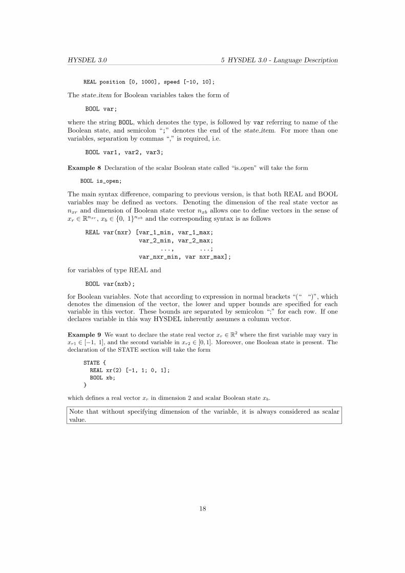
The main syntax difference, comparing to previous version, is that both REAL and BOOLvariables may be defined as vectors. Denoting the dimension of the real state vector asnxr and dimension of Boolean state vector nxb allows one to define vectors in the sense ofxr ∈ R
nxr , xb ∈ {0, 1}nxb and the corresponding syntax is as follows
REAL var(nxr) [var_1_min, var_1_max;
var_2_min, var_2_max;
..., ...;
var_nxr_min, var nxr_max];
for variables of type REAL and
BOOL var(nxb);
for Boolean variables. Note that according to expression in normal brackets “(“ “)”, whichdenotes the dimension of the vector, the lower and upper bounds are specified for eachvariable in this vector. These bounds are separated by semicolon “;” for each row. If onedeclares variable in this way HYSDEL inherently assumes a column vector.
Example 9 We want to declare the state real vector xr ∈ R2 where the first variable may vary in
xr1 ∈ [−1, 1], and the second variable in xr2 ∈ [0, 1]. Moreover, one Boolean state is present. Thedeclaration of the STATE section will take the form
STATE {
REAL xr(2) [-1, 1; 0, 1];
BOOL xb;
}
which defines a real vector xr in dimension 2 and scalar Boolean state xb.
Note that without specifying dimension of the variable, it is always considered as scalarvalue.
18

HYSDEL 3.0 5 HYSDEL 3.0 - Language Description
5.3.3 OUTPUT section
In the OUTPUT section, output variables of the SYSTEM are to be declared. These variablescan be of type REAL (i.e. yr ∈ R), and BOOL (i.e. yb ∈ {0, 1}), similarly as in the INPUTand STATE section. In general, the syntax of the OUTPUT section is as follows
OUTPUT { output_item }
where each new output item is separated by at least one character space and differs for realand binary variables. The output item for real variables takes the form of
REAL var;
where the string REAL, which denotes the type, is followed by var referring to name of theoutput variable. More variables are delimited by commas “,” as in the INPUT and STATEsection.
Note that in the OUTPUT section no bounds are specified. It is because the output vari-able is always considered as an affine function of states and inputs, thus their bounds areautomatically inferred.
Example 10 Declaration of the scalar output variables called “y1” and “y2” will be as follows
REAL y1, y2;
where no bounds are specified.
The output item for Boolean variables takes the form of
BOOL var;
where the string BOOL, which denotes the type, is followed by var referring to name of theBoolean output, and semicolon “;” denotes the end of the output item. If there are moreoutput variables, they are delimited by commas “,”.
Example 11 Declaration of the scalar Boolean output variables “d1”, “d2”, and “d3” will takethe form
BOOL d1, d2, d3;
which is the same as in HYSDEL 2.0.5.
Comparing to previous version, output variables may be defined as vectors. Denoting thedimension of the real output vector as nyr and dimension of Boolean output vector nyb
allows one to define vectors in the sense of yr ∈ Rnyr , yb ∈ {0, 1}nyb and the corresponding
syntax is then straightforward
REAL var(nyr);
for variables of type REAL where nyr denotes the dimension and
BOOL var(nub);
for Boolean variables with nub specifying the dimension of the column vector.
Example 12 We want to declare the output real vector yr ∈ R2, the second output real vector
q ∈ R2 and one binary vector outputs d ∈ {0, 1}3
19

HYSDEL 3.0 5 HYSDEL 3.0 - Language Description
OUTPUT {
REAL yr(2), q(2);
BOOL d(3);
}
Note that declaring the binary output in vectorized form is similar to example 11, but in this caseis shorter.
5.3.4 PARAMETER section
The PARAMETER section declares variables which will be treated as constants throughwhole HYSDEL file structure. In this case the syntax of the PARAMETER section is asfollows
PARAMETER { parameter_item }
where each parameter item may take one of the following forms
• declaration of constant scalars
type var = value;
• declaration of constant column vectors with dimension n (the dimension does not haveto be present for constants)
type var = [value_1; value_2; ..., value_n];
• declaration of constant matrices with dimensions n×m (the dimension does not haveto be present for constants)
type var = [value_11, value_12, ..., value_1m;
value_21, value_22, ..., value_2m;
..., ..., ..., ...;
value_n1, value_n2, ..., value_nm];
where type can be either REAL or BOOL. If there are more parameters with constantvalues, they have to be separated using semicolons “;” as new variable, i.e.
type var1 = value1; type var2 = value2;
type var3 = value3;
Notations in vector and matrix description remain the same as in INPUT, STATE andOUTPUT section. That is, each element of the row is delimited with comma “,” and therow ends with semicolon “;” .
Example 13 We want to declare constants a = 1 as Boolean variable, b = [−1, 0.5, −7.3]T and
D =
(
−1 0 0.230.12 −0.78 2.1
)
as real variables. This can be done as follows
PARAMETER {
BOOL a = 1; REAL b = [-1; 0.5; -7.3];
REAL D = [-1, 0, 0.23; 0.12, -0.78, 2.1];
}
20
HYSDEL 3.0 5 HYSDEL 3.0 - Language Description
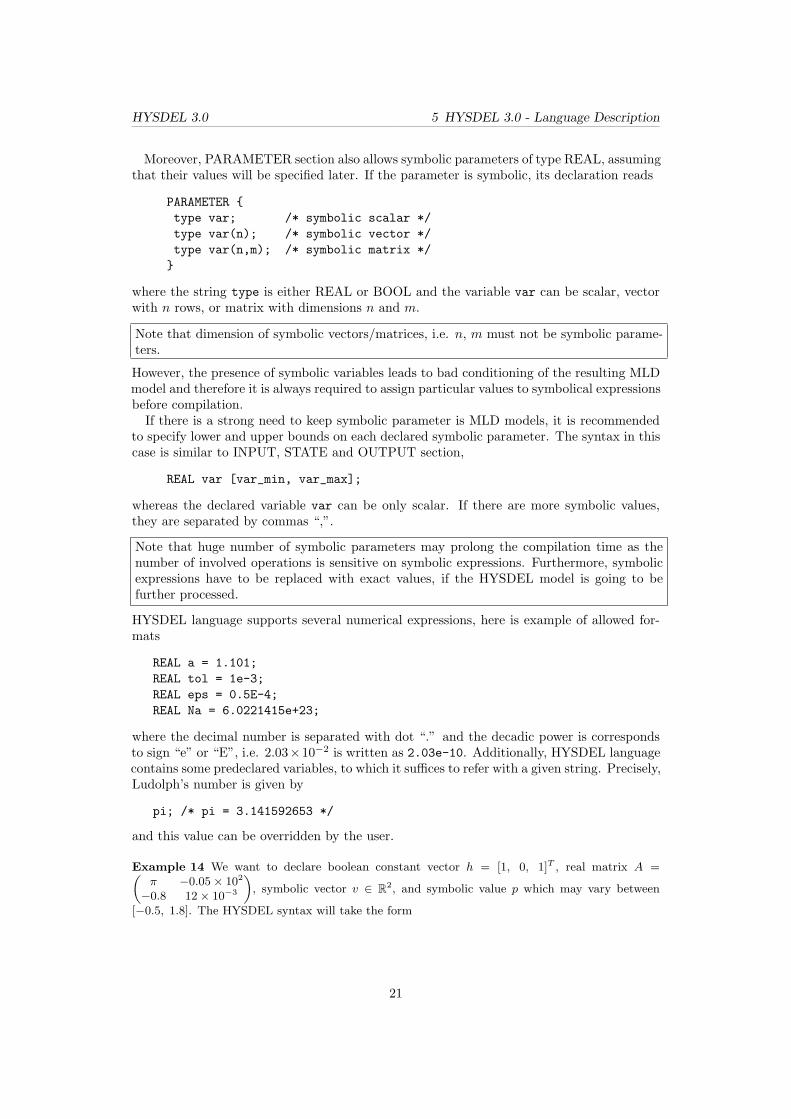
Moreover, PARAMETER section also allows symbolic parameters of type REAL, assumingthat their values will be specified later. If the parameter is symbolic, its declaration reads
PARAMETER {
type var; /* symbolic scalar */
type var(n); /* symbolic vector */
type var(n,m); /* symbolic matrix */
}
where the string type is either REAL or BOOL and the variable var can be scalar, vectorwith n rows, or matrix with dimensions n and m.
Note that dimension of symbolic vectors/matrices, i.e. n, m must not be symbolic parame-ters.
However, the presence of symbolic variables leads to bad conditioning of the resulting MLDmodel and therefore it is always required to assign particular values to symbolical expressionsbefore compilation.If there is a strong need to keep symbolic parameter is MLD models, it is recommended
to specify lower and upper bounds on each declared symbolic parameter. The syntax in thiscase is similar to INPUT, STATE and OUTPUT section,
REAL var [var_min, var_max];
whereas the declared variable var can be only scalar. If there are more symbolic values,they are separated by commas “,”.
Note that huge number of symbolic parameters may prolong the compilation time as thenumber of involved operations is sensitive on symbolic expressions. Furthermore, symbolicexpressions have to be replaced with exact values, if the HYSDEL model is going to befurther processed.
HYSDEL language supports several numerical expressions, here is example of allowed for-mats
REAL a = 1.101;
REAL tol = 1e-3;
REAL eps = 0.5E-4;
REAL Na = 6.0221415e+23;
where the decimal number is separated with dot “.” and the decadic power is correspondsto sign “e” or “E”, i.e. 2.03×10⁻² is written as 2.03e-10. Additionally, HYSDEL languagecontains some predeclared variables, to which it suffices to refer with a given string. Precisely,Ludolph’s number is given by
pi; /* pi = 3.141592653 */
and this value can be overridden by the user.
Example 14 We want to declare boolean constant vector h = [1, 0, 1]T , real matrix A =(
π −0.05× 10²
−0.8 12× 10−3
)
, symbolic vector v ∈ R2, and symbolic value p which may vary between
[−0.5, 1.8]. The HYSDEL syntax will take the form
21

HYSDEL 3.0 5 HYSDEL 3.0 - Language Description
PARAMETER {
BOOL h = [1; 0; 1]; /* constant vector */
REAL A = [pi, -0.05e2; -0.8, 12E-3]; /* constant matrix */
REAL v(2); /* symbolic vector */
REAL p [-0.5, 1.8]; /* symbolic scalar with given bounds */
}
Note that before evaluating the MLD structure, it is necessary to assign particular values to symbolicparameters, otherwise HYSDEL reports an error.
5.3.5 MODULE section
The MODULE section is a new feature of HYSDEL 3.0 which allows to create subsystems.This is important especially when creating larger HYSDEL structures. To be able to rec-ognize which subsystem is a part of which system a concept of master and slave files isadopted. A slave file will be referred to as a system, which is a part of bigger system, hasits own inputs, outputs and acts independently. A master file consist of at least one slavefile while inputs and outputs are created by subsystems.
Example 15 Example of a standard HYSDEL slave file, without any subsystems (i.e. without theMODULE section)
SYSTEM valve {
/* example of slave HYSDEL file referring to a valve */
INTERFACE {
/* declaration of variables */
INPUT { ... }
STATE { ... }
OUTPUT { ... }
PARAMETER { ... }
}
IMPLEMENTATION {
/* relations between declared variables */
}
}
The syntax of the MODULE section is given by
MODULE { module_item }
where each of the module item is composed of
name par;
The string name refers to a name of the subsystem which contains parameter par. If thereare more parameters, they are separated by commas, i.e.
name par1, par2, par3;
The syntax is similar to defining symbolical parameters in the PARAMETER section whilethe exact values have to be assigned in the PARAMETER section before compilation.
Example 16 Assume that the SYSTEM “valveA” creates together with SYSTEM “valveB” asystem called tank. Since both systems are similar, we will treat them as parameters of one file“valve”. The corresponding syntax of the master file in HYSDEL language will look as follows
22

HYSDEL 3.0 5 HYSDEL 3.0 - Language Description
SYSTEM tank {
/* example of master HYSDEL file referring to a tank comprised of two valves */
INTERFACE {
/* declaration of variables */
MODULE {
valve valveA, valveB;
}
INPUT { ... }
STATE { ... }
OUTPUT { ... }
PARAMETER { ... }
}
IMPLEMENTATION {
/* relations between declared variables */
}
}
where the string valve is the name of the subsystem with parameters valveA and valveB.
The syntax of the master file tank.hys indicates that both of the valves valveA, valveB areparameters of one slave file valve.hys created in the same directory. Overall behavior ofthe system is now described by this master file and the directory listing is shown in Fig. 5.1.Remember that before compilation, the exact values of the parameters valveA and valveB
needs to be assigned.If the file tank.hys is a part of another system, say it belongs to a storage unit, then this
file becomes a slave of the master file, called e.g. storage unit etc. Obviously, such nestingcan continue up the desired level.
Figure 5.1: Example of a SYSTEM tank containing two subsystems valveA, valveB and corre-
sponding directory listing.
For instance if one wants to model a production system which consists of several subsystemsthe syntax will look as follows
SYSTEM production {
INTERFACE {
MODULE {
storage_tank tank1, tank2;
conveyor_belt belt;
packaging packer;
}
/* other section are omitted */
}
23

HYSDEL 3.0 5 HYSDEL 3.0 - Language Description
where the slave files are determined via name of the subsystem and corresponding files. Thisparticular example is explained in section 5.5, on page 38.
5.4 IMPLEMENTATION Section
Relations between variables are determined in the IMPLEMENTATION section. Accordingto type of variables, this section is further partitioned into subsections, which remain thesame as in previous version. Syntactical structure of the IMPLEMENTATION section hasthe following form
IMPLEMENTATION { implementation_item }
which comprises of curly brackets and implementation item. The implementation item maytake only following forms
AUX { /* aux_item */ }
CONTINUOUS { /* continuous_item */ }
AUTOMATA { /* automata_item */ }
LINEAR { /* linear_item */ }
LOGIC { /* logic_item */ }
AD { /* ad_item */ }
DA { /* da_item */ }
MUST { /* must_item */ }
OUTPUT { /* output_item */ }
where each item appears only once in this section. Each implementation item is separatedat least with one space character and may be omitted, if it is not required. The order ofeach item can be arbitrary, it does not play a role for further processing.
Note that OUTPUT section is also present as in the INTERFACE part but here it hasdifferent syntax and semantics.
New changes in the IMPLEMETATION section affect the syntax of each subsection andthe common features are listed as follows:
• indexing
• FOR and nested FOR loops
• operators and built-in functions
These changes will be explained first, before describing the individual changes in each IN-TERFACE subsection.
Example 17 A structure of the standard HYSDEL file is given next where the meaning of eachsubsection of the IMPLEMENTATION part is briefly explained
SYSTEM name {
INTERFACE {
/* declaration of variables, subsystems */
}
IMPLEMENTATION {
/* relations between declared variables */
AUX {
24

HYSDEL 3.0 5 HYSDEL 3.0 - Language Description
/* declaration of auxiliary variables, needed for
calculations in the IMPLEMENTATION section */
}
CONTINUOUS {
/* state update equation for variables of type REAL */
}
AUTOMATA {
/* state update equation for variables of type BOOL */
}
LINEAR {
/* linear relations between variables of type REAL */
}
LOGIC {
/* logical relations between variables of type BOOL */
}
AD {
/* analog-digital block, specifying relations between
variables of type REAL to BOOL */
}
DA {
/* digital-analog block, specifying relations between
variables of type BOOL to REAL */
}
MUST {
/* specification of input/state/output constraints */
}
OUTPUT {
/* selection of output variables which can be of type
REAL or BOOL) */
}
}
}
5.4.1 Indexing
Introducing vectors and matrices induced the extension of the HYSDEL language to useindexed access to internal variables. The syntax is different for vectors and matrices since itdepends on the dimension of the variable. Access to vectorized variables has the followingsyntax
new_var = var(ind);
where new var denotes the name of the auxiliary variable (must be defined in AUX section),var is the name of the internal variable and ind is a vector of indices, referring to positionof given elements from a vector. Indexing is based on a Matlab syntax, where the argumentind must contain only N+ = {1, 2, . . .} valued elements and its dimension is less or equalto dimension of the variable var. Syntax of the ind vector can be one of the following:
• increasing/decreasing sequence
ind_start:increment:ind_end
where ind start denotes the starting position of indexed element, increment is thevalue of which the starting value increases/decreases, and ind end indicates the endposition of indexed element.
25

HYSDEL 3.0 5 HYSDEL 3.0 - Language Description
• increasing by one sequence
ind_start:ind_end
where the value increment is now omitted and HYSDEL automatically treats thevalue as +1
• particular positions
[pos_1, pos_2, ..., pos_n]
where pos 1, ..., pos n indicates the particular position of elements
• nested indices
ind(sub_ind)
where the vector ind is sub-indexed via the aforementioned ways by vector sub ind
with N+ values
Example 18 In the parameter section were defined two variables. The first variable is a constantvector h = [−0.5, 3, 1, π, 0]T and the second variable is a symbolical expression g ∈ R
3, g1 ∈[−1, 1], g2 ∈ [−2, 2], g3 ∈ [−3, 3]. We want to assign new variables z and v for particular elementsof these vectors. Examples are:
• increasing sequence, e.g. z = [−0.5, 1, 0]T
z = h(1:2:5);
• decreasing sequence, e.g. v = [g3, g2]T
v = g(3:-1:2);
• increasing by one, e.g. z = [1, π, 0]T
z = h(3:5);
• particular positions, e.g. v = [g1, g3]T
v = g([1,3]);
• nested indexing, e.g. z = [3, π]T , k = [2, 3, 4]
z = h(k([1, 3]));
where the variable k has to be declared first.
Indexing of matrices is similar, however, in this case two indices are required. The indexedsyntax takes the following form
new_var = var(ind_row,ind_col);
where new var denotes the name of the auxiliary variable (must be defined in AUX section),var is the name of the internal variable, ind row is a vector of indices referring to rows, andind col is a vector of indices referring to columns.
Note that indexing is based on a Matlab syntax, where the argument ind must contain onlyN+ = {1, 2, . . .} valued elements and its dimension is less or equal to dimension of thevariable var.
Syntax of the items ind row, ind col is the same as for vectors the item ind.
26

HYSDEL 3.0 5 HYSDEL 3.0 - Language Description
Example 19 In the parameter section a constant matrix is defined
A =
0 −5 −0.8 1−2 0.3 0.6 −1.20.5 0.1 −3.2 −1
We may extract values from matrix A to form new variable B as follows
• increasing sequence, e.g.
B =
(
0 −5−2 0.3
)
B = A(1:2,1:2);
• decreasing sequence, e.g.
B =
0.5 0.1 −3.2 −1−2 0.3 0.6 −1.20 −5 −0.8 1
B = A(3:-1:1,1:4);
• particular positions, e.g. B = [0, 0.3, −3.2]T
B = A(1:3,[1, 2, 3]);
• nested indexing, e.g. B = [0.6, −1.2]T , irow = [2, 3], icol = [1, 2, 3, 4]
B = h(i_row,i_col(3:4));
where the variables i row and i col have to be declared first.
5.4.2 FOR loops
FOR loops are another important feature of HYSDEL 3.0 version. To create a repeatedexpression, one has to first define an iteration counter in the AUX section according tosyntax
AUX {
INDEX iter;
}
where the prefix INDEX denotes the class, and iter is the name of the iteration variable. Ifthere are more iteration variables required, the additional variables are separated by commas“,”, i.e.
AUX {
INDEX iter1, iter2, iter3;
}
As the iteration variable is declared, the FOR syntax takes the form of
FOR ( iter = ind ) { repeated_expr }
where the string FOR is followed by expression in normal brackets “(”, “)” and expressionin curly brackets “{”, “}”. The expression in normal brackets is characterized by assign-ment iter = ind where the iteration variable iter incrementally follows the set defined byvariable ind and this variable takes one of the form shown in section indexing 5.4.1. Theexpression in curly brackets named repeated expr is recursively evaluated for each value ofiterator iter and can take the form of
27

HYSDEL 3.0 5 HYSDEL 3.0 - Language Description
aux_item
continuous_item
automata_item
linear_item
logic_item
ad_item
da_item
must_item
output_item
depending in which section the FOR loop lies. This allows to use the FOR loop within thewhole IMPLEMENTATION section.
Example 20 Suppose, that it is required to repeat ad item in the AD section for each binaryvariable di if state xri ≥ 0, i = 1, 2, 3, i.e.
d1 = xr1 ≥ 0
d2 = xr2 ≥ 0
d3 = xr3 ≥ 0
The iteration index, as well as auxiliary Boolean variable d has to defined first,
AUX {
INDEX i;
BOOL d(3);
}
and they can be consequently used in the AD section as follows
AD {
FOR (i=1:3) { d(i) = xr(i) >= 0; }
}
HYSDEL 3.0 supports also nested loops. In this case the syntax remains the same, butthe repeated expr has now the structure of
FOR ( iter = ind ) { repeated_expr }
which does not differ from the syntax outlined above.
Example 21 Suppose that we want to code a matrix multiplication for state update equation ofthe form
(
xr1(k + 1)xr2(k + 1)
)
=
(
1 0.50.2 0.9
)(
xr1(k)xr2(k)
)
+
(
10
)
ur(k)
Assuming that vectors x, u are already declared, we also declare constant matrices in the INTER-FACE section
PARAMETER {
REAL A = [1, 0.5; 0.2, 0.9];
REAL B = [1; 0];
}
Secondly, we define iteration counters in IMPLEMENTATION section
AUX {
INDEX i,j;
}
28

HYSDEL 3.0 5 HYSDEL 3.0 - Language Description
and then use the nested loop syntax as follows
CONTINUOUS {
FOR (i=1:2) {
x(i) = 0;
FOR (j=1:2) { x(i) = A(i,j)*x(j) + x(i); }
x(i) = x(i) + B(i)*u;
}
}
Example 22 FOR loops allow also to more complicated expressions. For instance, indexing in apower sequence 2i where i = 1, . . . , 5. Assume that for given vector h ∈ R
32 it is required to assigna real variable z ∈ R
5 according to power sequence indexing. In HYSDEL it can be written asfollows
FOR (i=1:5) { z(i) = h(2^i); }
where the variables i, z, and h were previously declared.
5.4.3 HYSDEL operators and built-in functions
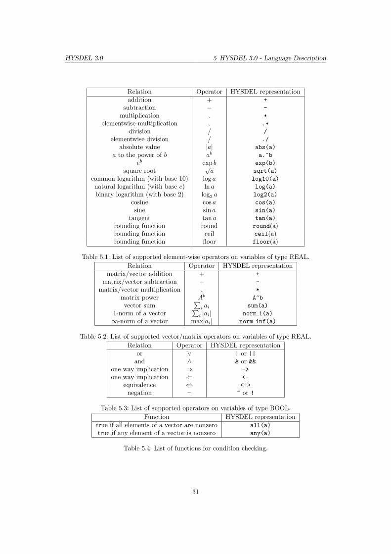
Throughout the whole HYSDEL file various relations between variables can be defined.Because the variables may be also vectors (matrices), the list of supported operators isdistinguished by
• element-wise operations, in Tab. 5.1
• and vector functions, in Tab. 5.2.
For Boolean variables HYSDEL supports operators, as summarized in Tab. 5.3. Additionally,syntactical functions are available, which allow condition checking and are summarized inTab. 5.4.Since the variables may be constants as well as varying, the operators cannot be used
arbitrary. This holds especially for varying variables of type REAL (states, inputs, outputs,auxiliary). Denoting this group with notation v, only following relations are allowed
• relations between varying variables v1 and v2 of type REAL
– addition: v1 + v2
– subtraction: v1 - v2
• relations between varying variable v and constant parameter p of type REAL
– addition: v + p = p+ v (v and p have the same dimension)
– subtraction: v − p = −p+ v (v and p have the same dimension)
– multiplication: v ∗ p = p ∗ v (p is scalar)
– division: v/p = 1/p ∗ v (p is scalar except 0)
• operations summarized in tables 5.1, 5.2, and 5.4 hold for relations between two pa-rameters p1, p2 of type REAL
• for variables of type BOOL are only Boolean expressions valid (Tab. 5.3. However,operations of type REAL can be used but only if the Boolean variable is retyped toclass REAL.
29

HYSDEL 3.0 5 HYSDEL 3.0 - Language Description
If in the expression two or more operators appear, their evaluation is according to operatorpriority. That is for instance, v = a+ b ∗ c will have the result is v = a+ (b ∗ c). In general,it is recommended to use normal brackets “(“, “)” to separate variables into groups andevaluate bracketed and hence prior expressions first.
Note that nonlinear operators are not allowed for any state/input/output and auxiliaryvariables and HYSDEL 3.0 will report an error whenever such case occurs.
5.4.4 Casting Boolean to real
Using the keyword
(REAL Boolean_var)
it is possible to cast a Boolean variable Boolean var into a real variable. This functionallows to operate with binary variables using operators defined for variables of class REAL.
Example 23 Suppose that in the INTERFACE section a Boolean variable was declared
INPUT { BOOL d(2);}
and we want to use it for operations with real numbers. The cast operator
x = x + (REAL d);
treats both Boolean inputs d as real variables.
If one wants to retype a Boolean expression into a real number, this can be done by definingauxiliary logic variable in LOGIC section and apply the cast operator for this auxiliaryvariable.
Example 24 Suppose that one wants to recast the expression d1&d2 to a class REAL. Firstly, anadditional variable needs to be created in LOGIC section, e.g.
LOGIC { d = d1 & d2; }
and afterward, the cast operator can be applied to this variable, e.g.
CONTINUOUS { x = 2.3*(REAL d) - 0.5*u; }
5.4.5 AUX section
In the AUX section one has to declare auxiliary variables needed for derivations of furtherrelations in the IMPLEMENTATION section. The declaration of these variables followswith specifying the type of the variable (REAL, BOOL or INDEX) and defining the name,e.g.
type var;
where the string type can be REAL, BOOL or INDEX and it is followed by a variable var.If there are more variables, they are delimited by commas “,”. Declaration of vectors usesthe same syntax as mentioned in INPUT/STATE/OUTPUT section.
Note that whenever there is a FOR loop in HYSDEL file, the looping variable has to bedefined here as INDEX.
30
HYSDEL 3.0 5 HYSDEL 3.0 - Language Description
Relation Operator HYSDEL representationaddition + +
subtraction − -
multiplication . *
elementwise multiplication . .*
division / /
elementwise division / ./
absolute value |a| abs(a)
a to the power of b ab a.^b
eb exp b exp(b)
square root√a sqrt(a)
common logarithm (with base 10) log a log10(a)
natural logarithm (with base e) ln a log(a)
binary logarithm (with base 2) log2 a log2(a)
cosine cos a cos(a)
sine sin a sin(a)
tangent tan a tan(a)
rounding function round round(a)rounding function ceil ceil(a)rounding function floor floor(a)
Table 5.1: List of supported element-wise operators on variables of type REAL.
Relation Operator HYSDEL representationmatrix/vector addition + +
matrix/vector subtraction − -
matrix/vector multiplication . *
matrix power Ab A^b
vector sum∑
i ai sum(a)
1-norm of a vector∑
i |ai| norm 1(a)
∞-norm of a vector max|ai| norm inf(a)
Table 5.2: List of supported vector/matrix operators on variables of type REAL.
Relation Operator HYSDEL representationor ∨ | or ||and ∧ & or &&
one way implication ⇒ ->
one way implication ⇐ <-
equivalence ⇔ <->
negation ¬ ~ or !
Table 5.3: List of supported operators on variables of type BOOL.
Function HYSDEL representationtrue if all elements of a vector are nonzero all(a)
true if any element of a vector is nonzero any(a)
Table 5.4: List of functions for condition checking.
31
HYSDEL 3.0 5 HYSDEL 3.0 - Language Description
Example 25 Suppose that in the AUX section we have to declare two iterators i, j, two realvectors z ∈ R
3, v ∈ R2 and Boolean variable d ∈ {0, 1}5. The AUX syntax takes the following form
AUX {
INDEX i,j; /* iteration counters */
REAL z(3),v(2); /* auxiliary REAL vectors */
BOOL d(5); /* auxiliary BOOL vector */
}
Contrary to INTERFACE section, here lower and upper bounds on the variables are notgiven. The values are automatically calculated from variables declared in the INTERFACEsection since AUX variables are affine functions of these variables. Moreover, no constants,as well as no parameters are here declared.
5.4.6 CONTINUOUS section
In the CONTINUOUS section the state update equations for variables of type REAL are tobe defined. The general syntax is given as
CONTINUOUS { continuous_item }
where the continuous item may be inside a FOR loop and takes the form
var = affine_expr;
The variable var corresponds to the state variable declared in the section STATE and itcan be scalar or vectorized expression. The affine expr is an affine function of parameters,inputs, states and auxiliary variables, which have been previously declared.
Note that only variables of type REAL, declared in STATE section can be assigned here.
Example 26 Suppose that the state update equation is driven by
x(k + 1) = Ax(k) +Bu(k) + f
where the matrices A, B, f are constant parameters, x is state, u is input. This can be written inHYSDEL language as short vectorized form, i.e.
CONTINUOUS {
x = A*x + B*u + f;
}
5.4.7 AUTOMATA section
The AUTOMATA section describes the state transition equations for variables of typeBOOL. The general syntax takes the form
AUTOMATA { automata_item }
where the automata item may be inside a FOR loop and is built by
var = Boolean_expr;
32

HYSDEL 3.0 5 HYSDEL 3.0 - Language Description
The variable var corresponds to the Boolean variable defined in the section STATE andit can be scalar or vectorized expression. The Boolean expr is a combination of Booleaninputs, Boolean states, and auxiliary Boolean variables with operators reported in Tab. 5.3.
Note that only variables of type BOOL, declared in STATE section can be assigned here.
Example 27 Suppose that the Boolean state update is driven by following relations
x2(k + 1) = u1(k) ∨ (u2(k) ∧ ¬x1(k))
Related HYSDEL syntax will take the form of
AUTOMATA {
xb(2) = ub(1) | (ub(2) & ~xb(1));
}
5.4.8 LINEAR section
In the LINEAR section it is allowed to define additional variables, which are build by affineexpressions of states, inputs, parameters and auxiliary variables of type REAL. In general,the structure of the LINEAR section is given by
LINEAR { linear_item }
where the linear item may be inside a FOR loop and takes the form of
var = affine_expr;
The variable var is of type REAL and was previously declared in the AUX section. Theaffine expr is an affine function of parameters, inputs, states and auxiliary variables of typeREAL, which have been previously declared.
Example 28 Consider that it is suitable to define an auxiliary continuous variable g = −0.5x1 +3which is an affine function of the state x ∈ R
2. The variable is firstly declared in the AUX section,
AUX {
REAL g;
}
and consequently, the expression in LINEAR section takes the form
LINEAR {
g = -0.5*x(1) + 3;
}
Furthermore, the LINEAR section is devoted to determine relations between subsystemsand applies only if there is MODULE section present. More precisely, the syntax is given by
var = affine_expr;
where the variable var access the internal input or output variable of type REAL of the de-clared subsystem. The affine expr is an affine function of internal inputs or output variablesof type REAL of the declared subsystems. More detailed view for merging of subsystemswill be given in special section.
Note that LINEAR section serves also for declaration of interconnection between subsystems(if they are declared in MODULE section).
33

HYSDEL 3.0 5 HYSDEL 3.0 - Language Description
5.4.9 LOGIC section
LOGIC section allows to define additional relations between variables of type BOOL whichmight simplify the overall notations. In general the syntax is given by
LOGIC { logic_item }
where the logic item may be inside a FOR loop and is built by
var = Boolean_expr;
The variable var corresponds to the Boolean variable defined in the section AUX and it canbe scalar or vectorized expression. The Boolean expr is a combination of Boolean inputs,Boolean states, and auxiliary Boolean variables with operators reported in Tab. 5.3.
Example 29 Suppose that we want to introduce the Boolean variable d = x1 ∧ (¬x2 | ¬x3), whichis a function of Boolean states x ∈ {0, 1}3. We proceed first with variable declaration in AUXsection
AUX {
BOOL d;
}
and follow with LOGIC section
LOGIC {
d = x(1) & (~x(2) | ~x(3));
}
5.4.10 AD section
AD section is used to express the relations between variables of type REAL to Booleanvariables only with help of logical operator equivalence. Here, the equivalence operator <->
is replaced with = operator and the syntax is given as
AD { ad_item }
where the ad item might be inside a FOR loop and it can be one of the following
var = affine_expr > real_num;
var = affine_expr >= real_num;
var = affine_expr < real_num;
var = affine_expr <= real_num;
var = affine_expr == real_num;
The variable var is of type BOOL and has to be declared in the AUX section. Theaffine expr is a function of states, inputs, parameters and auxiliary variables of type REAL.Operator >= or > denotes the greater or equal inequality (≥), operator <= or < is less orequal inequality (≤), and operator == stands for equality constraint. Expression real numis a real valued number.
Note that whenever a binary variable is associated to equality constraint, this assignment isnumerically sensible, and it might lead to unexpected results.
34

HYSDEL 3.0 5 HYSDEL 3.0 - Language Description
Example 30 Suppose that we want to assign to a Boolean variable d ∈ {0, 1}3 value 1 if certaininequality is satisfied, otherwise it will be 0.
d1 =
{
1 if x1 + 2u2 ≥ 0
0 otherwise, d2 =
{
1 if 0.5x2 − 3x3 ≤ 0
0 otherwise, d3 =
{
1 if x1 ≥ 1.2
0 otherwise
HYSDEL allows to model this behavior using AD syntax
AUX {
BOOL d(3);
}
AD {
d(1) = x(1) + 2*u(2) >= 0;
d(2) = 0.5*x(2) - 3*x(3) <= 0;
d(3) = x(1) >= 1.2;
}
Previous version required bounds on auxiliary variables var in the form of
var = affine_expr >= real_num [min, max, eps];
var = affine_expr <= real_num [min, max, eps];
but this syntax is obsolete and related bounds calculation are now obtained automatically.If the bounds will be provided anyway, HYSDEL will raise a warning.
Note that AD section does not use curly brackets “{“, “}” to assign the auxiliary variable.
5.4.11 DA section
The DA section defines continuous variables according to if-then-else conditions. HYSDEL3.0 language supports the following syntax
DA { da_item }
where the da item might be inside a FOR loop or and it can be one of the following
var = { IF cond THEN affine_expr };
var = { IF cond THEN affine_expr ELSE affine_expr};
The variable var corresponds to auxiliary variable of type REAL, defined in the AUX section.Expression cond can be defined as
affine_expr > real_num;
affine_expr >= real_num;
affine_expr < real_num;
affine_expr <= real_num;
affine_expr == real_num;
Boolean_expr;
which denotes certain condition satisfaction. The affine expr is a function of states, inputs,parameters and auxiliary variables of type REAL. Operator >= or > denotes the greateror equal inequality (≥), operator <= or < is less or equal inequality (≤) and == standsfor equality constraint (which is numerically very sensible). Expression real num is a realvalued number. The Boolean expr is a function of Boolean states, inputs, parameters andauxiliary variables combined with operators listed in Tab. 5.3.w
Note that if the ELSE string is missing, HYSDEL automatically treats the value equal 0.
35

HYSDEL 3.0 5 HYSDEL 3.0 - Language Description
Example 31 Suppose that we want to introduce an auxiliary variable z which depends on a con-tinuous state x and a binary input ub as follows
z =
{
x if ub = 1
−x if ub = 0
HYSDEL models this relation by
AUX {
REAL z;
}
DA {
z = { IF ub THEN x ELSE -x };
}
Example 32 It is also possible to define switching conditions using real expressions. Suppose thatwe want to introduce an auxiliary variable z which depends on continuous states x1 and x2
z =
{
2x1 if x2 ≥ 0
−x1 + 0.5x2 if x2 ≤ 0
HYSDEL 3.0 allows to models this relation by
AUX {
REAL z;
}
DA {
z = { IF x(2) >= 0 THEN 2*x(1) ELSE -x(1)+0.5*x(2) };
}
and this syntax is more familiar to describe the behavior of piecewise affine systems.
Similarly as in the AD section, previous version required bounds on variables
var = { IF cond THEN affine_expr [min, max, eps] };
var = { IF cond THEN affine_expr [min, max, eps]
ELSE affine_expr [min, max, eps] };
This syntax is obsolete and related bounds calculation is now performed automatically.HYSDEL will report a warning if this syntax will be used.
5.4.12 MUST section
MUST section specifies constraints on input, state, and output variables. Regardless of thetype of variables, it is required that these condition will be fulfilled for the whole time. TheMUST section takes the following syntax
MUST { must_item }
where the must item can be one of the following
real_cond;
Boolean_expr;
real_cond BO Boolean_expr;
Boolean_expr BO real_cond;
36

HYSDEL 3.0 5 HYSDEL 3.0 - Language Description
which denotes certain condition satisfaction. Expression real cond is given by
affine_expr > real_num;
affine_expr >= real_num;
affine_expr < real_num;
affine_expr <= real_num;
affine_expr == real_num;
and BO is a Boolean operator from Tab. 5.3. The affine expr is a function of states, inputs,parameters and auxiliary variables of type REAL. Operator >= or > denotes the greateror equal inequality constraint (≥), operator <= or < is less or equal inequality constraint(≤), and == is an equality constraint. Expression real num is a real valued number. TheBoolean expr is a function of Boolean states, inputs, parameters and auxiliary variablescombined with operators listed in Tab. 5.3.
Example 33 Consider a system where the one input real variable ur ∈ R and five states xr ∈ R5.
Moreover, although the bounds on these variables have been declared, additional constraints areintroduced, which are subsets of the declared bounds, i.e. ur ∈ [−2, 2] and xr1 ∈ [−1, 5], xr2 ∈[−2, 3.4], xr3 ∈ [0.5, 2.8]. These constraints are written in MUST section as follows
MUST {
ur >= -2;
ur <= 2;
xr(1:3) >= [-1; -2; 0.5];
xr(1:3) <= [5; 3.4; 2.8];
}
Example 34 For binary variables, one way implications are allowed, as well as equivalence. Ex-ample is a system with binary inputs ub ∈ {0, 1}2 which implies that a value of auxiliary binaryvariable will be 0 or 1, e.g.
d1 ⇒ ub1, d2 ⇐ ub2, d3 ⇔ xb2
and it can be written in HYSDEL as
MUST {
d(1) -> ub(1);
d(2) <- ub(2);
d(3) <-> xb(2);
}
Example 35 HYSDEL 3.0 supports also combined REAL–BOOL expressions. Consider a statevector x ∈ R
2, and binary input ub ∈ {0, 1}2. One may require the constraints as
ub1 ⇒ x1 ≥ 0,
x1 + 2x2 ≥ −2 ⇐ ¬ub2,
ub1 ∨ ub2 ⇔ x1 − x2 ≥ 1
and it can be written in HYSDEL as
MUST {
ub(10) -> x(1) >= 0;
x(1) + 2*x(2) <- ~ub(2);
(ub(1) | ub(2)) <-> x(1) - x(2) >= 1;
}
Note that when combining Boolean expr with real cond it is recommended to use normalbrackets “()” for bracketing the Boolean expr, in order to avoid non-correct compilation.
37
HYSDEL 3.0 5 HYSDEL 3.0 - Language Description
5.4.13 OUTPUT section
The OUTPUT section specifies the output variables for the overall MLD system. Outputvariables can be both of type REAL and BOOL. The following syntax is accepted
OUTPUT { output_item }
where the output item might be inside a FOR loop and it can be one of the following
var = affine_expr;
var = Boolean_expr;
The variable var corresponds to a variable declared in INTERFACE part, OUTPUT sectionwhich is either of type REAL and BOOL. According to its type, the affine expr is assignedto REAL output and Boolean expr is assigned to Boolean output.
Example 36 Suppose that current system has both real xr and Boolean states xb. If we want towrite output equations to these states, e.g.
yr = xr
yb = xb
the HYSDEL syntax takes the form of
OUTPUT {
yr = xr;
yb = xb;
}
Note that in OUTPUT section it is not allowed to assign other output variables, as declaredin OUTPUT section in INTERFACE part.
5.5 Merging of HYSDEL Files
This section introduces a new feature available in HYSDEL 3.0 which allows merging ofhysdel files to subsystems. Initial information about merging was given in the MODULEsection but here is this topic explained more in details.
5.5.1 Creating slave files
Similarly as all the variables, subsystems needs to be declared first too. For this purposea new section of INTERFACE part is created called MODULE. Here are the subsystemsdeclared according their name and containing parameters, as explained in section 5.3.5. Sub-systems are independent HYSDEL files with given names, inputs, outputs, states, parametersand are contained in the same directory as the master file.Consider a simple production system which is built by two storage tanks, one conveyor belt
and a packaging unit, as illustrated in Fig. 5.2. The task is to model the whole production unitusing MLD system. First at all the production unit is virtually separated into subsystems,as shown in Fig. 5.3 and the connections between the subsystems are clarified. Now it isclear which file should be regarded as slave and which as master. We shall call the masterfile production and at first sight it seems that one would declare four slave files, e.g.
1. tank1
38

HYSDEL 3.0 5 HYSDEL 3.0 - Language Description
Figure 5.2: Illustrative example of a production system, composed from different parts.
Figure 5.3: The production unit can be represented by four subsystems with corresponding
connections.
2. tank2
3. belt
4. packer
but because tanks tank1 and tank2 have the same dynamics, it is better to treat theseobjects as parameters of one file. Subsequently, we can group these both tanks into one fileand end up in only three subsystems, e.g.
1. storage tank
2. conveyor belt
3. packaging
where each of the objects is now an individual hys-file and can contain arbitrary number ofparameters. Declaration of these subsystems in HYSDEL will take a form
MODULE {
storage_tank tank1, tank2;
conveyor_belt belt;
packaging packer;
}
and it corresponds to three HYSDEL files which will be included, i.e.
39

HYSDEL 3.0 5 HYSDEL 3.0 - Language Description
1. storage tank.hys
2. conveyor belt.hys
3. packaging.hys
Each of these file is a slave file. For instance, the file storage tank.hys may be written inHYSDEL language as follows
SYSTEM storage_tank {
INTERFACE {
STATE { REAL level; }
INPUT { REAL u; }
OUTPUT { REAL y; }
PARAMETER {
REAL diameter;
REAL k=1e-2;
}
}
IMPLEMENTATION {
CONTINUOUS { level = 0.9*level+1/diameter*(u-k*level);}
OUTPUT { y = level; }
}
}
where we decided to keep one parameter as symbolic. This is important, as it allows to defineonly one hys-file which can be used several times for different values of this parameter, thusreferring to multiple objects. Similarly, we create other slave files, in particular
SYSTEM conveyor_belt {
INTERFACE {
STATE { REAL speed [0, 6]; }
INPUT { BOOL sw; }
OUTPUT { REAL y; }
PARAMETER {
REAL k=[0.5, 0.1];
}
}
IMPLEMENTATION {
AUX { REAL z; }
DA { z = {IF sw THEN k(1)*speed+2*(REAL sw) ELSE k(2)*speed }; }
CONTINUOUS { speed = z; }
OUTPUT { y = speed; }
}
}
and
SYSTEM packaging {
INTERFACE {
INPUT { REAL inflow [0, 50]; }
OUTPUT { REAL outflow; }
}
40
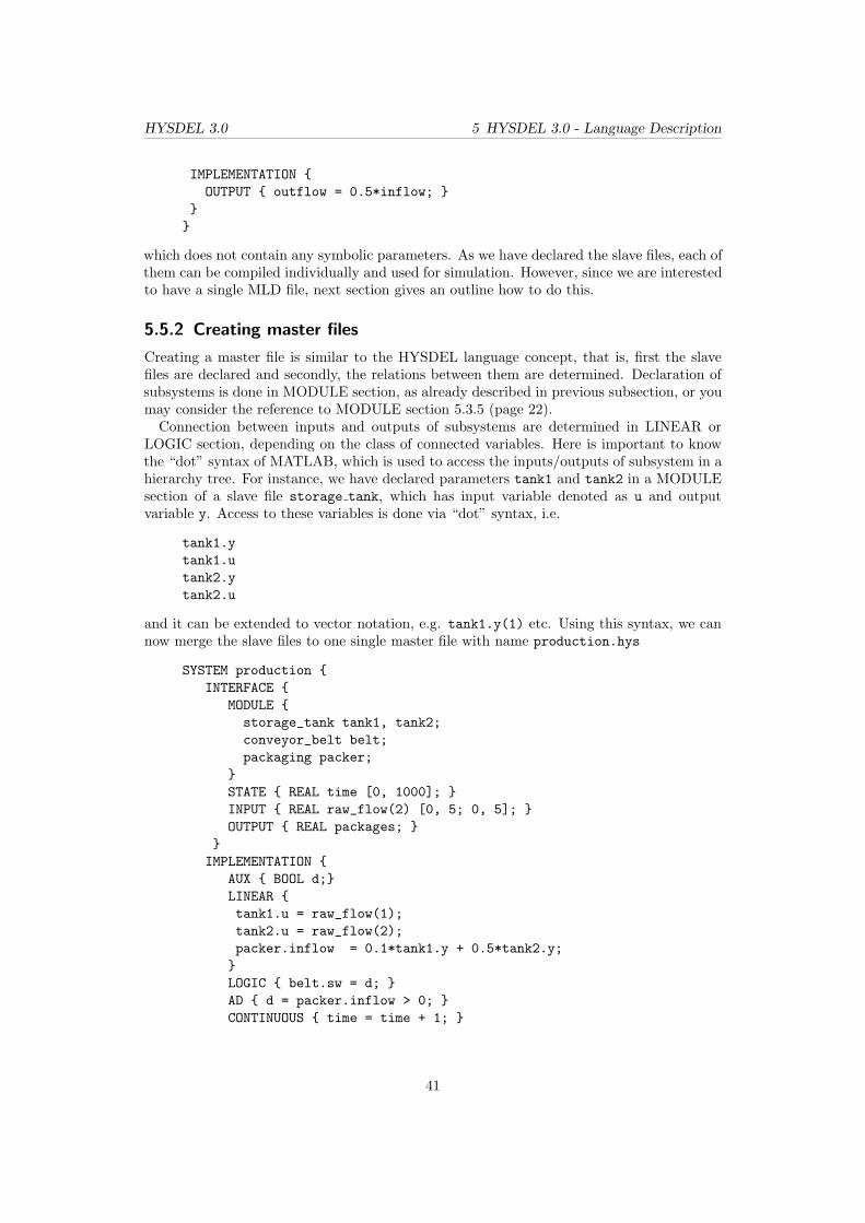
HYSDEL 3.0 5 HYSDEL 3.0 - Language Description
IMPLEMENTATION {
OUTPUT { outflow = 0.5*inflow; }
}
}
which does not contain any symbolic parameters. As we have declared the slave files, each ofthem can be compiled individually and used for simulation. However, since we are interestedto have a single MLD file, next section gives an outline how to do this.
5.5.2 Creating master files
Creating a master file is similar to the HYSDEL language concept, that is, first the slavefiles are declared and secondly, the relations between them are determined. Declaration ofsubsystems is done in MODULE section, as already described in previous subsection, or youmay consider the reference to MODULE section 5.3.5 (page 22).
Connection between inputs and outputs of subsystems are determined in LINEAR orLOGIC section, depending on the class of connected variables. Here is important to knowthe “dot” syntax of MATLAB, which is used to access the inputs/outputs of subsystem in ahierarchy tree. For instance, we have declared parameters tank1 and tank2 in a MODULEsection of a slave file storage tank, which has input variable denoted as u and outputvariable y. Access to these variables is done via “dot” syntax, i.e.
tank1.y
tank1.u
tank2.y
tank2.u
and it can be extended to vector notation, e.g. tank1.y(1) etc. Using this syntax, we cannow merge the slave files to one single master file with name production.hys
SYSTEM production {
INTERFACE {
MODULE {
storage_tank tank1, tank2;
conveyor_belt belt;
packaging packer;
}
STATE { REAL time [0, 1000]; }
INPUT { REAL raw_flow(2) [0, 5; 0, 5]; }
OUTPUT { REAL packages; }
}
IMPLEMENTATION {
AUX { BOOL d;}
LINEAR {
tank1.u = raw_flow(1);
tank2.u = raw_flow(2);
packer.inflow = 0.1*tank1.y + 0.5*tank2.y;
}
LOGIC { belt.sw = d; }
AD { d = packer.inflow > 0; }
CONTINUOUS { time = time + 1; }
41

HYSDEL 3.0 5 HYSDEL 3.0 - Language Description
OUTPUT { packages = packer.outflow; }
MUST {
tank1.level <= 100;
tank2.level <= 80;
}
}
}
where all the sub-connections are declared in LINEAR and LOGIC section. Note thatthe master file production.hys has its own inputs and outputs and these are assignedto subsystems via “dot” syntax. Furthermore, we can access the state variables of singlesubsystems and do additional operations with them ( e.g. adding constraints as given inMUST section of production.hys file).After all the involved sub-connections in the master file are declared, one can proceed
with compilation of the master file
>> hysdel3(’production’)
Creating instance "tank1" of "storage_tank"...
Creating instance "tank2" of "storage_tank"...
Creating instance "belt" of "conveyor_belt"...
Creating instance "packer" of "packaging"...
and HYSDEL 3.0 generates an m-file equivalent of the input file (here production.m).The generated m-file is a YALMIP code, written as a function which accepts a structure ofparticular values for given symbolic parameters and outputs the MLD form. Since we havedeclared symbolic variable diameter in the slave file storage tank.hys, it is necessary toassign a particular value to this variable before calling the YALMIP code. This is done via“dot” syntax, referring to particular instances of overall master file, i.e.
>> par.tank1.diameter = 1;
>> par.tank2.diameter = 2;
Secondly, we can call the function with the parameter par
>> production(par)
and it returns the MLD representation for a given production system depicted in Fig. 5.2.The procedure for generating the MLD form of the master file can be done simple on a
graphical level as long the source master file production.hys is available. For this purpose,we copy the standard HYSDEL block from HYSDEL 3.0 Simulink library to a new schemeand fill all the required fields as shown in Fig. 5.4. After confirming the OK option, HYS-DEL automatically compiles the source file and generates a subsystem with correspondinginput/output ports. Consequently, we can add other blocks to the scheme and the resultmight look as given in Fig. 5.4. By pressing START button in Simulink, the simulationof MLD system should output the number of packages generated for given input raw flow,which is illustrated in Fig. 5.5.
5.5.3 Automatic generation of master files
HYSDEL 3.0 offers a routine for automatic generation of master files. This feature exploitsthe graphical way of creating subsystems, as given in Simulink. The subsystem can begenerated in Simulink by selecting multiple “HYSDEL Model” blocks and selecting the
42
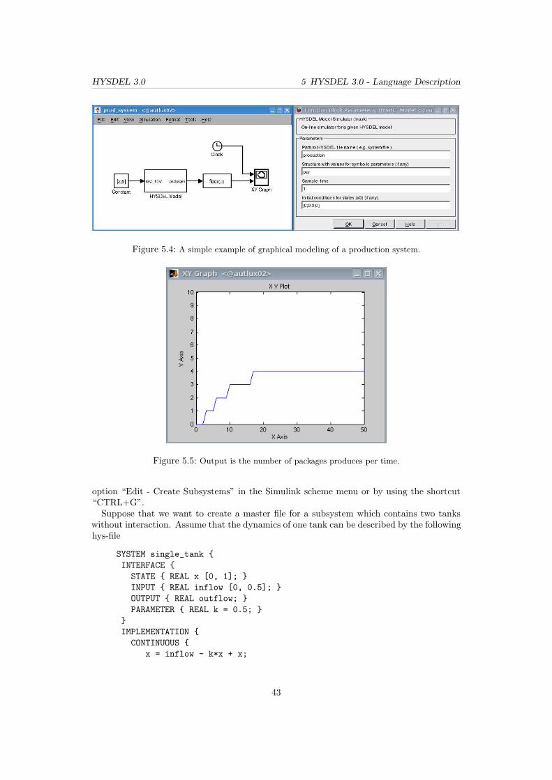
HYSDEL 3.0 5 HYSDEL 3.0 - Language Description
Figure 5.4: A simple example of graphical modeling of a production system.
Figure 5.5: Output is the number of packages produces per time.
option “Edit - Create Subsystems” in the Simulink scheme menu or by using the shortcut“CTRL+G”.Suppose that we want to create a master file for a subsystem which contains two tanks
without interaction. Assume that the dynamics of one tank can be described by the followinghys-file
SYSTEM single_tank {
INTERFACE {
STATE { REAL x [0, 1]; }
INPUT { REAL inflow [0, 0.5]; }
OUTPUT { REAL outflow; }
PARAMETER { REAL k = 0.5; }
}
IMPLEMENTATION {
CONTINUOUS {
x = inflow - k*x + x;
43

HYSDEL 3.0 5 HYSDEL 3.0 - Language Description
}
OUTPUT {
outflow = k*x;
}
}
}
which contains one input and output of class REAL. Firstly, we need to copy the “HYSDELModel” block from the HYSDEL 3.0 library to a new Simulink scheme and to create twoblocks for each tank. Secondly, we connect these blocks using arrows which represent thedata flow, as shown in Fig. 5.6. Afterward we create a subsystem containing both blockswith tanks and the result might look as in Fig. 5.7. The master file for this subsystem canbe obtained using the command
>> h3_sim2hys(’untitled/two_tanks’)
where the argument of the function h3 sim2hys is a path to subsystem. In this particularexample this path is given by the name of the current Simulink scheme followed by a backslashand the name of the subsystem block. This is the standard path used in MATLAB to referfor any Simulink block and the number of backslashes in the path denotes the hierarchylevel. Examples of the path can be obtained by selecting the desired Simulink block andusing one the following MATLAB commands
>> path1 = gcs % get name of the current Simulink system
>> path2 = gcb % get name of the current Simulink block
By using h3 sim2hys command, HYSDEL 3.0 detects names of the blocks in the subsys-tem, names of the subsystems and names of the hys-files which HYSDEL blocks refer to.Depending on the structure of the subsystems, the MODULE section in the master file iscreated as given by hierarchy of the subsystems. For this example, the master files has thefollowing form
SYSTEM two_tanks {
/* Automatically generated master file for HYSDEL3 */
/* Created at: 02-Jun-2008. */
INTERFACE {
INPUT {
REAL inflow;
}
OUTPUT {
REAL outflow;
}
MODULE {
single_tank T1, T2;
}
}
IMPLEMENTATION {
LINEAR {
T2.inflow = T1.outflow;
T1.inflow = inflow;
}
OUTPUT {
44

HYSDEL 3.0 5 HYSDEL 3.0 - Language Description
outflow = T2.outflow;
}
}
}
where names of the “HYSDEL Model” blocks are parsed to MODULE section and intercon-nections are parsed into LOGIC section. The name of the master file is given by the name ofsubsystem, i.e. two tanks.hys and this file is created in the current directory. If the parsedsubsystem contains more subsystems, the h3 sim2hys creates so many master files, as it isgiven by the hierarchy of subsystems.
Figure 5.6: Two tanks without interactions.
Figure 5.7: A subsystem containing two tanks.
5.6 EXAMPLES
5.6.1 Simple code
Example 37 Consider a static system with one binary input and the output is a negation of input
SYSTEM neg_single {
45
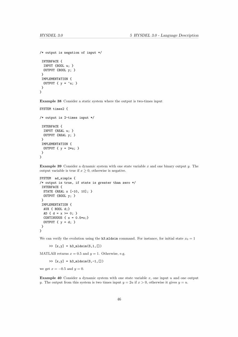
HYSDEL 3.0 5 HYSDEL 3.0 - Language Description
/* output is negation of input */
INTERFACE {
INPUT {BOOL u; }
OUTPUT {BOOL y; }
}
IMPLEMENTATION {
OUTPUT { y = ~u; }
}
}
Example 38 Consider a static system where the output is two-times input
SYSTEM times2 {
/* output is 2-times input */
INTERFACE {
INPUT {REAL u; }
OUTPUT {REAL y; }
}
IMPLEMENTATION {
OUTPUT { y = 2*u; }
}
}
Example 39 Consider a dynamic system with one state variable x and one binary output y. Theoutput variable is true if x ≥ 0, otherwise is negative.
SYSTEM ad_simple {
/* output is true, if state is greater than zero */
INTERFACE {
STATE {REAL x [-10, 10]; }
OUTPUT {BOOL y; }
}
IMPLEMENTATION {
AUX { BOOL d;}
AD { d = x >= 0; }
CONTINUOUS { x = 0.5*x;}
OUTPUT { y = d; }
}
}
We can verify the evolution using the h3 mldsim command. For instance, for initial state x0 = 1
>> [x,y] = h3_mldsim(S,1,[])
MATLAB returns x = 0.5 and y = 1. Otherwise, e.g.
>> [x,y] = h3_mldsim(S,-1,[])
we get x = −0.5 and y = 0.
Example 40 Consider a dynamic system with one state variable x, one input u and one outputy. The output from this system is two times input y = 2u if x > 0, otherwise it gives y = u.
46
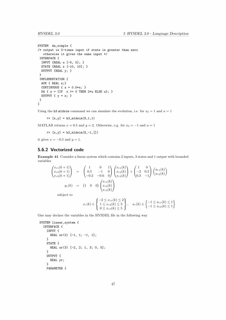
HYSDEL 3.0 5 HYSDEL 3.0 - Language Description
SYSTEM da_simple {
/* output is 2-times input if state is greater than zero
otherwise it gives the same input */
INTERFACE {
INPUT {REAL u [-5, 5]; }
STATE {REAL x [-10, 10]; }
OUTPUT {REAL y; }
}
IMPLEMENTATION {
AUX { REAL z;}
CONTINUOUS { x = 0.5*x; }
DA { z = {IF x >= 0 THEN 2*u ELSE u}; }
OUTPUT { y = z; }
}
}
Using the h3 mldsim command we can simulate the evolution, i.e. for x0 = 1 and u = 1
>> [x,y] = h3_mldsim(S,1,1)
MATLAB returns x = 0.5 and y = 2. Otherwise, e.g. for x0 = −1 and u = 1
>> [x,y] = h3_mldsim(S,-1,[])
it gives x = −0.5 and y = 1.
5.6.2 Vectorized code
Example 41 Consider a linear system which contains 2 inputs, 3 states and 1 output with boundedvariables
xr1(k + 1)xr2(k + 1)xr3(k + 1)
=
1 0 10.5 −1 0−0.2 −0.6 0
xr1(k)xr2(k)xr3(k)
+
1 0−2 0.50.3 −1
(
ur1(k)ur2(k)
)
yr(k) =(
1 0 0)
xr1(k)xr2(k)xr3(k)
subject to
xr(k) ∈
−2 ≤ xr1(k) ≤ 21 ≤ xr2(k) ≤ 30 ≤ xr3(k) ≤ 5
, ur(k) ∈
{
−1 ≤ ur1(k) ≤ 1−1 ≤ ur2(k) ≤ 1
}
One may declare the variables in the HYSDEL file in the following way
SYSTEM linear_system {
INTERFACE {
INPUT {
REAL ur(2) [-1, 1; -1, 1];
}
STATE {
REAL xr(3) [-2, 2; 1, 3; 0, 5];
}
OUTPUT {
REAL yr;
}
PARAMETER {
47

HYSDEL 3.0 5 HYSDEL 3.0 - Language Description
REAL A = [1, 0, 1; 0.5, -1, 0; -0.2, -0.6, 0];
REAL B = [1, 0; -2, 0.5; 0.3, -1];
REAL C = [1, 0, 0];
}
IMPLEMENTATION {
CONTINUOUS {
xr = A*xr + B*ur;
}
OUTPUT {
yr = C*xr;
}
}
}
Example 42 Consider HYSDEL 3.0 code for a general linear systems
x(k + 1) = Ax(k) +Bu(k)
where x ∈ Rn, u ∈ R
m, y ∈ Rp. In this case it is easier to keep all parameters symbolic and specify
it later. A HYSDEL 3.0 code may look as follows
SYSTEM ltiABCmnp {
/* all parameters are kept as symbolic */
INTERFACE {
INPUT { REAL u(m) [-5, 5];}
STATE { REAL x(n) [-5, 5]; }
OUTPUT { REAL y(p); }
PARAMETER { REAL A,B,C,m,n,p; }
}
IMPLEMENTATION {
CONTINUOUS { x = A*x + B*u; }
OUTPUT { y = C*x; }
}
}
Example 43 Consider a PWA system as given in [2], which contains one input, two states, twooutputs and two linear dynamics defined over two partitions
x(k + 1) =
{
A1x(k) +B1u(k) if x1(k) > 0
A2x(k) +B2u(k) if x1(k) < 0
The HYSDEL 3.0 code can be written as follows:
SYSTEM pwa_sincos {
INTERFACE {
PARAMETER {
REAL A1 = [0.4, 0.6928; -0.6928, 0.4];
REAL A2 = [0.4, -0.6928; 0.6928, 0.4];
REAL B = [0; 1];
}
INPUT { REAL u [-1, 1]; }
STATE { REAL x(2) [-10, 10]; }
48

HYSDEL 3.0 5 HYSDEL 3.0 - Language Description
OUTPUT { REAL y(2); }
}
IMPLEMENTATION {
AUX { REAL z(2); }
DA { z = {IF x(1)<0 THEN A1*x+B*u ELSE A2*x+B*u}; }
CONTINUOUS { x = z;}
OUTPUT { y = x; }
}
}
5.6.3 Advanced code
Example 44 Consider that we want to design a predictive controller for a simple linear system.Next example shows how it is possible using various enhancements in HYSDEL 3.0 syntax.
SYSTEM mpc_linear {
/* MPC for the linear double integrator */
INTERFACE {
STATE {
REAL X(nx, 1) [-10, 10]; /* initial state */
}
INPUT {
REAL U(nu, N) [-1, 1]; /* N-1 dimensional matrix of inputs,
i.e. [U_0 U_1 .. U_(N-1)] */
}
OUTPUT {
REAL y; /* one system output - 1st element of the last predicted state */
}
PARAMETER {
REAL N = 5; /* prediction horizon */
REAL nx = 2, nu = 1; /* number of states, number of inputs */
REAL A = [1, 1; 0, 1]; /* x(k+1) = A*x + B*u */
REAL B(2,1) = [1; 0.5]; /* x(k+1) = A*x + B*u */
}
}
IMPLEMENTATION {
AUX {
REAL z(nx, N+1); /* nx-by-N dimensional matrix of predicted states */
INDEX i; /* index variable */
}
LINEAR {
z(1:nx, 1) = X(1:nx); /* z(:,1) = X_0 */
/* here we model the system evolution x(k+1) = A*x(k) + B*u(k) */
FOR (i = 1:N) {
z(1:nx, i+1) = A*z(1:nx, i) + B*U(1:nu, i);
}
}
CONTINUOUS {
/* next state update corresponds to last predicted state, i.e. to X_N */
X = z(1:nx, N+1);
}
OUTPUT {
/* system output is the 1st element of the last predicted state */
49

HYSDEL 3.0 5 HYSDEL 3.0 - Language Description
y = X(1);
}
MUST {
/* all elements of predicted states constrained between +10 and -10 */
z <= 10;
z >= -10;
}
}
}
Example 45 This example illustrates the design of an predictor used in hybrid predictive controland it features advanced HYSDEL 3.0 syntax.
SYSTEM mpc_pwa {
/* MPC for the famous sin-cos PWA system */
INTERFACE {
STATE {
REAL X(nx, 1) [-10, 10]; /* initial state, nx-by-1 vector */
}
INPUT {
REAL U(nu, N) [-1, 1]; /* N-1 dimensional matrix of system inputs */
}
OUTPUT {
REAL y; /* system output, identical to 1st element of last state */
}
PARAMETER {
REAL N = 5; /* prediction horizon */
REAL nx = 2, nu = 1; /* number of states, number of inputs */
/* matrices of system dynamics */
REAL A1 = [0.4, 0.6928; -0.6928, 0.4], A2 = [0.4, -0.6928; 0.6928, 0.4];
REAL B(2,1) = [0; 1];
}
}
IMPLEMENTATION {
AUX {
REAL z(nx, N+1); /* N-by-nx matrix, corresponds to X_0, X_1, ..., X_N */
BOOL negative(N); /* N-1 dimensional vector of delta variables */
INDEX i; /* index variable */
}
LINEAR {
z(1:nx, 1) = X(1:nx); /* set z(:, 1) = X_0 */
}
AD {
/* negative_1 = z(1, 1) <= 0,
negative_2 = z(1, 2) <= 0,
negative_3 = z(1, 3) <= 0,
...
negative_(N-1) = z(1, N-1) <= 0
*/
FOR (i = 1:N) {
negative(i) = z(1, i) <= 0;
}
}
DA {
50

HYSDEL 3.0 5 HYSDEL 3.0 - Language Description
/* PWA dynamics. x(k+1) = A1*x(k) + B*u(k) if "negative(k)" is true,
otherwise x(k+1) = A2*x(k) + B*u(k)
*/
FOR (i = 1:N) {
z(1:nx, i+1) = {IF negative(i) THEN A1*z(1:nx, i) + B*U(1:nu, i)
ELSE A2*z(1:nx, i) + B*U(1:nu, i)};
}
}
CONTINUOUS {
/* next state update corresponds to last predicted state, i.e. to X_N */
X = z(1:nx, N+1);
}
OUTPUT {
/* system output is the 1st element of the last predicted state */
y = X(1);
}
MUST {
/* all elements of every predicted state constrained between +10 and -10 */
z <= 10;
z >= -10;
}
}
}
51

6 Control design with HYSDEL 3.0
This chapter explains various ways how to use the MLD models of HYSDEL 3.0 for designinga predictive controller. To synthesize a controller, higher level tools are adopted, such asYALMIP and MPT Toolbox.
6.1 Export of MLD system to PWA model
Once the MLD structure is available in MATLAB workspace, one can use it in several ways,including simulation of hybrid systems, or control design. An excellent tool for designingcontrol for hybrid systems is MPT toolbox [5]. It has incorporated many functions whichcan even process the HYSDEL 2.0.5 source code and use it directly for control design. Forfurther details, please consult MPT manual or MATLAB help to mpt sys function.
However, as HYSDEL 3.0 has newer syntax, the function mpt sys has to deal with ex-tended syntax of the HYSDEL 3.0 -files. Due to this reason, another routine was imple-mented in HYSDEL 3.0 , which processes the new MLD format (3.2) and outputs MPTsysStruct format. The principle of conversion is based on an equivalence between differentforms of hybrid system [3]. One of the forms, as used in MPT Toolbox, is given by piecewiseaffine (PWA) system
x(k + 1) = Aix(k) +Biu(k) + fi if (x(k), u(k)) ∈ Di (6.1)
where Ai, Bi, fi are state update matrices defined over polyhedral regions
Di ={
(x(k), u(k)) ∈ Rnx+nu Hx,ix(k) +Hu,iu(k) ≤ Ki, i = 1, . . . , nD
}
(6.2)
defined in x − u space. The number nD denotes the total number of partitions. An effi-cient transformation from MLD description to PWA system has been shown in [1], and thealgorithm is implemented in function h3 mld2pwa. The use of this function is as follows
>> sysStruct = h3_mld2pwa(S)
where the input argument is the HYSDEL 3.0 MLD structure and the output is the MPTsysStruct format. For help, type
>> help mpt_sysStruct
and MPT toolbox gives you options how to work with this format.
Note that h3 mld2pwa uses MPT/polytope library and for a proper use of this function,MPT toolbox has to be installed.
Example 46 Suppose that we want to obtain a PWA representation of a simple hybrid modelof car. The dynamics of a car is given by three states position, velocity, turbocount and theswitching between two hybrid modes (normal mode/turbo mode) is given by an external binaryinput turbo. The source file might be given as follows:
52

HYSDEL 3.0 6 Control design with HYSDEL 3.0
SYSTEM turbo_car {
INTERFACE {
STATE {
REAL position [-50, 50];
REAL velocity [-10, 10];
REAL turbocount [-10, 10];
}
INPUT {
REAL acc [-1, 1];
BOOL turbo;
}
OUTPUT {
REAL y;
}
}
IMPLEMENTATION {
AUX {
REAL aux_acc;
}
DA {
aux_acc = {IF turbo THEN 2*acc ELSE acc};
}
CONTINUOUS {
position = position + velocity + aux_acc;
velocity = velocity + 0.5*aux_acc;
turbocount = turbocount - (REAL turbo);
}
OUTPUT {
y = position;
}
}
}
In MPT Toolbox, it is possible to get a PWA representation simply using
>> mpt_sys(’turbo_car’)
command. Alternatively, we can use the HYSDEL 3.0 to get the MLD representation first, i.e.
>> hysdel3(’turbo_car’)
>> S = turbo_car
Secondly, the PWA form can be obtained by
>> sysStruct = h3_mld2pwa(S)
which can be used for control design in MPT Toolbox. For instance, to obtain an explicit controllerwhich drives the car to a position 30, can be achieved by defining a problem structure probStruct
(see MATLAB help)
>> probStruct.N = 3;
>> probStruct.Q = [1 0.5 0];
>> probStruct.R = [1 0];
>> probStruct.norm = 1;
>> probStruct.subopt_lev = 0;
>> probStruct.xref = [30; 0; 0];
53

HYSDEL 3.0 6 Control design with HYSDEL 3.0
and invoking the main routine
>> ctrl = mpt_control(sysStruct, probStruct);
Resulting controller is stored in a MPT-structure and to simulate a closed loop we need to use otherfunctions of MPT Toolbox, such as
>> mpt_plotTimeTrajectory(ctrl,[0;0;0],20)
which returns a plot shown in Fig. 6.1.
0 5 10 15 20−10
0
10
20
30
40Evolution of states
Sampling Instances
Sta
tes
0 5 10 15 200
5
10
15
20
25
30
35Evolution of outputs
Sampling Instances
Outp
uts
0 5 10 15 20−1
−0.5
0
0.5
1Evolution of control moves
Sampling Instances
Inputs
0 5 10 15 201
1.2
1.4
1.6
1.8
2Active dynamics
Sampling Instances
Dynam
ics
x1
x2
x3
y1
u1
u2
Figure 6.1: A closed loop simulation for a turbo car model as returned by MPT Toolbox.
54

Bibliography
[1] A. Bemporad. Efficient conversion of mixed logical dynamics systems into an equivalentpiecewise affine form. IEEE Trans. on Aut. Control, 49(5):832–838, 2004.
[2] A. Bemporad and M. Morari. Control of Systems Integrating Logic, Dynamics, andConstraints. Automatica, 35(3):407–427, march 1999.
[3] W.P.M.H. Heemels, B. De Schutter, and A. Bemporad. Equivalence of hybrid dynamicalmodels. Automatica, (37):1085–1091, 2001.
[4] M. Kvasnica. Efficient software tools for control and analysis of hybrid systems. PhDthesis, ETH Zurich, Switzerland, February 2008.
[5] M. Kvasnica, P. Grieder, and M. Baotic. Multi-Parametric Toolbox (MPT), 2004. Avail-able at http://control.ee.ethz.ch/~mpt/.
[6] J. Loefberg. http://control.ee.ethz.ch/∼joloef/wiki/pmwiki.php.
[7] J. Lofberg. Yalmip : A toolbox for modeling and optimization in MATLAB. InProceedings of the CACSD Conference, Taipei, Taiwan, 2004. Available at http:
//control.ee.ethz.ch/~joloef/yalmip.php.
[8] F. Torrisi and A. Bemporad. HYSDEL-a tool for generating computational hybrid modelsfor analysis and synthesis problems. IEEE Transactions on Control Systems Technology,12(2):235–249, 2004.
[9] F. Torrisi, A. Bemporad, G. Bertini, P. Hertach, D. Jost, and D. Mignone. HYSDEL2.0.5 User manual. Zurich, September, 2002.
55