I , .

I . I I I I I c I I 1 I I I I I 1 c I I

Rensselaer Polytechnic I n s t i t u t e

Troy, New Ynrk

FINALF3RlRT PARTC

GRANT no. NGR-33-018-

NATIONAL AERONAUTICS

AND SPACE ADMINISTRATION

SENSITIVITY DESIGN TECHNIQUE

FOR OFTIMAL CONTROL

Submitted on behalf of

Rob Roy

Associate Professor of E l e c t r i c a l Engineering

Co-Investigator: J. H. Ri l l ings

October 1967

https://ntrs.nasa.gov/search.jsp?R=19680009798 2020-03-12T09:27:28+00:00ZCORE Metadata, citation and similar papers at core.ac.uk

Provided by NASA Technical Reports Server

Introduction

This report describes a f e a s i b i l i t y study conducted t o investigate the

poss ib i l i t y of using optimal s ens i t i v i ty design techniques t o design a feed-

back control system for a large, f lexible booster. The vehicle t o be controlled

i s described i n NASA MSFC "Model Vehicle No. 2". The design objective i s t o

maintain the vehicle i n the immediate neighborhood of a predefined nominal

t r a j ec to ry i n s p i t e of disturbances act ing on the vehicle.

are both external, such as random wind gusts, and in t e rna l such as changes i n

vehicle parameters.

of the vehicle within design l imits, preferably a s small a s possible.

These disturbances

An addi t ional design objective i s t o keep the bending

The nominal t r a j ec to ry of the vehicle i s described by a set of nonlinear

d i f f e r e n t i a l equations. However, small perturbations of the vehicle 's motion

about t he nominal can be adequately characterized by a set of l inear incre-

mental d i f f e r e n t i a l equations with time varying coeff ic ients .

t o calculate these coefficients were obtained from the "Model Vehicle No. 2"

data package.

The data needed

1

The Problem

The vehicle t o be controlled i s a large f l ex ib l e booster of the Saturn

type.

The control objectives can be divided in to categories -- r i g i d body objectives

and bending body objectives.

Control i s exerted by gimballing four of the eight propulsion engines.

The object of the r i g i d body control i s t o maintain the vehicle a s close

as possible t o i t s nominal t ra jec tory i n s p i t e of random wind gusts.

f irst approximation it i s assumedthat the necessary parameters of the f i c -

t i c i o u s r i g i d body can be measured exactly (c f . Fisher) .

A s a

2

-2 - Unfortunately, because the vehicle i s f lex ib le , t h i s r i g i d body is non-

ex is ten t .

t r o l l a b l e ) torque applied t o one end.

control torque for the r i g i d body exci tes bending modes i n t h e vehicle.

ignored, these osc i l l a t ions could reach a point where the vehicle exceeds

i t s e l a s t i c limits and i s destroyed.

vent t h i s .

experimental determinations of the values of t he parameters involved i n the

bending i s d i f f i c u l t . Thus, the successful control s t ra tegy must limit the

bending when the parameters are known only approximately and change with time.

For s implici ty only the first bending mode i s considered and i t s equation

i s assumed t o be that of a l i nea r o sc i l l a to r .

Rather t he vehicle behaves l i k e an unsupported beam with a (con-

Gimballing the engines t o provide a

If

A successful control s t ra tegy must pre-

Because of the large s ize of the vehicle, however, full scale

The r i g h t hand side of the equation i s the engine exc i ta t ion of the

Combining t h i s f irst bending mode with the r i g i d body descr ipt ion mode.

gives the vehicle descr ipt ion i n terms of f ive state variables.

I

0

I 0

0

0

0

0

e -u=

0

\

-2p 7

-3-

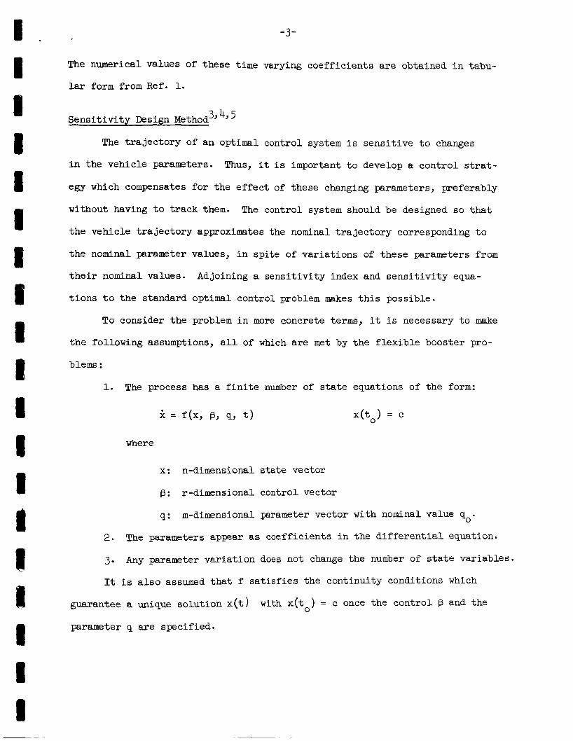
The numerical values Of these t i m e varying coeff ic ients are obtained i n tabu-

lar form from R e f . 1.

Sens i t i v i ty Design Method 3 4 5 ’ ’ The t r a j ec to ry of an optimal control system i s sens i t ive t o changes

i n the vehicle parameters. Thus, it is important t o develop a control strat-

egy which compensates for the e f f ec t of these changing parameters, preferably

without having t o t rack them. The control system should be designed s o t h a t

t h e vehicle t r a j ec to ry approximates the nominal t r a j ec to ry corresponding t o

the nominal parameter values, i n spi te of var ia t ions of these parameters from

their nominal values.

t i ons t o the standard optimal control problem mkes t h i s possible.

Adjoining a sens i t i v i ty index and s e n s i t i v i t y equa-

To consider the problem i n more concrete terms, it i s necessary t o make

t h e following assumptions, a l l of which are met by the f l ex ib l e booster pro-

blems :

1.

2.

3-

It

The process has a

k = f(x, p,

where

f i n i t e number of state equations of the form:

9, t ) x( to> = c

x: n-dimensional s t a t e vector

p: r-dimensional control vector

q: m-dimensional parameter vector with nominal value q . 0

The parameters appear as coeff ic ients i n the d i f f e r e n t i a l equation.

Any parameter var ia t ion does not change the number of state variables.

is a l s o assuned that f s a t i s f i e s the continuity conditions which

guarantee a unique solut ion x ( t >

parameter q are specified.

with x ( to ) = c once the control p and the

-4-

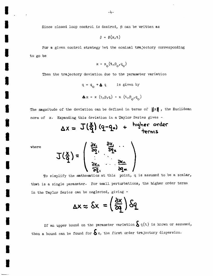
Since closed loop control i s desired, p can be wr i t ten as

B = B(x,t)

For a given control s t ra tegy l e t the nominal t r a j e c t o r y corresponding

t o go be

x = x 0 (t,B0,qo)

Then the t r a j ec to ry deviation due t o the parameter var ia t ion

9 = 9, + b 9 i s given by

The magnitude of the deviation can be defined i n terms of 11x11 , the Euclidean

norm of x. Expanding t h i s deviation i n a Taylor Ser ies gives -

where

Jy, =

t h a t i s a s ingle parameter.

i n t he Taylor Ser ies can be

For small perturbations, the higher order terms

neg,lected, giving -

n

ax, - * * - To simplify the mathematics a t t h i s point, q i s assumed t o be a scalar ,

If an upper bound on the parameter var ia t ion b q ( t ) i s known o r assumed,

then a bound can be found for &x, the f i rs t order t r a j ec to ry dispersion.

-5-

For su i tab ly small &q, then, Il&\\ can be l imited by l imit ing

At a point on the perturbed t ra jec tory (l$l> = %e+ At) the

s t a t e equations become

Expanding t h i s i n a taylor Series about (xn, q,) -

+ higher order terms

where f an i t s der ivat ives are evaluated a t (x 0,qo ). Again, f o r small

$q = (q - qo) the higher order terms a re negligible, leaving -

where s x is the f i r s t order approximation t o A x .

I f 6q i s a (known) bound on the parameter var ia t ion which yields the

maximum t r a j ec to ry dispersion b x, then, l e t t i n g z ( t ) 4s xllas above, the

s e n s i t i v i t y equation can be written as

This i s a l inear d i f f e ren t i a l equation defined on the nominal t ra jec-

-6-

tory.

limited, the nominal t ra jec tory and nominal control must be chosen t o l i m i t

z ( t ) .

cont ro l problem.

minimize t h e sum of the or ig ina l index of performance J and an index of sen-

s i t i v i t y J subject t o the constraints of the vehicle and the s e n s i t i v i t y

If t h e t r a j ec to ry dispersion due t o parameter var ia t ion i s t o be

This i s done by incorporating the sens i t i v i ty masure i n t o the optimal

To do t h i s the optimal control problem i s reformulated t o

equation.

The augmented optimal

determine

where

subject t o

control problem thus becomes

where f and g a re posit ive def in i te functions of x,v,p, and z. 0 0

Upon inspection it i s found tha t t h i s problem does not admit t o a solu-

t i o n as there i s no r e l a t ion which y i e l d s the s t r u c t u r a l information necessary

t o construct p*(t). Specif ical ly

specif ied.

t he form of a feedback control l a w . This completes the specif icat ion of the

problem and allows it t o be solved. The designer, however, must be judicious

i n h i s choice of feedback structure, since the resu l t ing "optimal" closed

loop system i s then optimal only with respect t o the spec i f ic type of feed-

back s t ruc ture specified.

&? i s unknown. The problem i s under-

Therefore, the designer imposes t h i s s t r u c t u r a l information i n b x

Two rather general s t ruc tures a re considered below.

-7-

Cascade Gains

Consider the control system shown i n Fig. 1. This consis ts of a s e t

of cascade gains w i t h u n i t feedback around the plant. The control l a w f o r

t h i s case i s

p(x,t) = K(v - X)

where K is the vector of feedback gains and v i s the desired state response.

The gains are t o be chosen t o reduce the s e n s i t i v i t y of t he nominal t ra jec-

t o ry t o parameter var ia t ions and t o keep the vehicle a s close t o t he nominal

t r a j ec to ry as possible.

Using t h i s control, the plant equation becomes -

and the s e n s i t i v i t y equation i s

Thus, the optimal control problem becomes

min (J + J) where K

subject t o the s t a t e and sens i t i v i ty equations.

The solut ion of t h i s problemby standard parameter optimization methods

gives a set of feedback gains K which i s r e a l l y a t rade off between the two

object ives of the problem. Two ta rge ts a re being aimed a t wi th only one arrow.

The next section improves on t h i s s i tua t ion .

Feedback Gains with Autonomous Input

Consider t he system of Fig. 2. This time control i s exerted by a set

-8 -

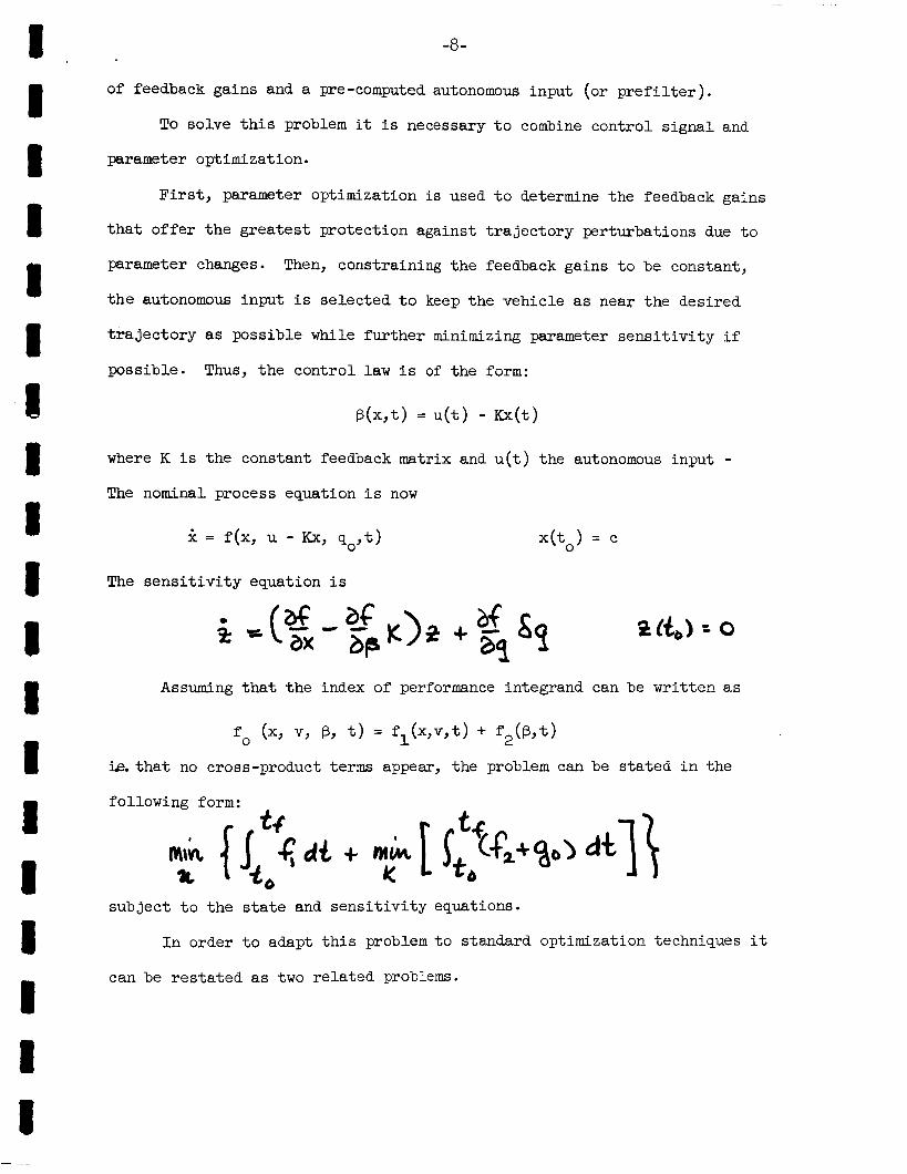
of feedback gains and a pre-computed autonomous input (or p r e f i l t e r ) .

To solve t h i s problem it i s necessary t o combine control s igna l and

parameter optimization.

F i r s t , parameter optimization is used t o determine the feedback gains

t h a t o f fe r t h e grea tes t protection against t r a j ec to ry perturbations due t o

parameter changes. Then, constraining the feedback gains t o be constant,

t h e autonomous input i s selected t o keep the vehicle as near the desired

t r a j ec to ry as possible while fur ther minimizing parameter s e n s i t i v i t y i f

possible. Thus, t he control l a w i s of the form:

where K i s the constant feedback matrix and u ( t ) the autonomous input - The nominal process equation i s now

2 = f(x, u - Kx, qo , t ) x ( to ) = c

The s e n s i t i v i t y equation i s

act,, = 0

Assuming t h a t t he index of performance integrand can be wri t ten as

f o (x, v, B, t> = f l ( X , V , t ) + f , ( B , t )

Le.that no cross-product terms appear, the problem can be stated i n the

subject t o the state and sens i t i v i ty equations.

I n order t o adapt t h i s problem t o standard optimization techniques it

can be r e s t a t ed as two re la ted problems.

-9-

1.

2.

Results

Feedback Gain Selection.

equations.

Autonomous Input Selection:

equations and k = 0.

The cascade gain configuration was solved on a d i g i t a l computer. Since

t h i s was a f e a s i b i l i t y study, weighting matrices were not selected t o give

the bes t possible resul ts , r a the r t he f i r s t weights t r i ed t h a t gave reason-

able results were used. With more time invested i n t h i s select ion r e s u l t s

should be be t t e r .

Figure 3 shows pi tch e r ro r and normalized bending for s ens i t i v i ty

weighting equal t o zero.

t i o n solut ion.

vehicle f o r nominal bending frequency, wo.

response f o r a -20% perturbation i n bending frequency.

case are not only much greater, but they exhibi t diverging osc i l la t ions .

This corresponds t o the usual parameter optimiza-

In both graphs the sol id l i n e indicates the response of the

The dotted l i n e indicates the

The er rors i n t h i s

Figure 4 shows the same quant i t ies with the sens i t i v i ty weighting in-

creased t o 10,000.

the results fo r nominal bending frequency are s l i g h t l y worse than those above.

However fo r t he -20% perturbation i n cu the r e s u l t s a re c lear ly grea t ly improved

and i n f ac t , qu i te acceptable.

Since the s t a t e and control weighting was not changed,

-10-

This study has proven the f e a s i b i l i t y of using optimal s e n s i t i v i t y

design techniques t o design a control system fo r a large, f l e x i b l e booster.

Work i s current ly underway t o use the techniques on a more sophis t icated

vehicle model where, f o r instance, s t a t e information is not d i r e c t l y ava i l -

able . Further development of the Feedback Gain Autonomous Input Technique

i s a l s o underway and t h i s is expected t o give even b e t t e r r e s u l t s than the

Cascade Gain Configuration.

CASCADE GAINS SYSTEM

FIGURE 1

1 I 1 I

FEEDBACK GAINS- PREFILTER SYSTEM

FIGURE 2

0.2

-

-0.2.

NORMALIZED BENDING

SENSITIVITY WTG = 0 - .08 rTCH (radians) ANGLE

FIGURE 3

SENSITIVITY WTG = lo5 1 4 PITCH ANGLE

FIGURE 4

DEFINITION OF SYMBOLS

F

K

1 C P

M

M1

N'

43

R '

U

v

V

X

X

y(x,)

Z

ot

ocw P 4 f ,

@I

Total thrust of Booster

Amplifier gain

Distance from engine gimbal t o vehicle center of gravi ty

Distance from vehicle center of gravi ty t o center of pressure

Total vehicle mass

Generalized mass of f irst bending mode

Aerodynamic force

(unknown) parameter

Control th rus t

Autonomous input

Reference input

Vehicle veloci ty

S ta t e vector

Drag Force

(output of p r e f i l t e r )

Normalized displacement a t engine gimbal

Sens i t iv i ty vector

Attack angle

Wind induced a t t ack angle

Engine gimbal angle

Atti tude angle

F i r s t bending mode damping

F i r s t bending mode amplitude

F i r s t bending mode frequency.

1 . .

I 8 I 1 I 1 I 1 I I I D 1 I I I I .I

REFERENCES

1. "Model Vehicle No. 2 fo r Advanced Control Studies" NASA-

MSFC In te rna l Document.

2. Fisher, E. E. "An Application of the Quadratic Penalty Function Cri ter ion

t o the Determination of a Linear Control for a Flexible Vehicle" AIAA

Journal, Vol 3 , No. 7 1965, pp. 1262-1267.

3 . Tomovic, R. Sens i t i v i ty Analysis of Dynamic System, McGraw-Hill, New

York, 1963.

4. Dougherty, H. "Synthesis of Optimal Feedback Control Systems Subject t o

Modelling Inaccuracies", Ph.D. Thesis, R.P.I., Troy, New York, February 1966.

5. Pagurek, B. "Sensi t ivi ty of the Performance of Optimal Control Systems

t o Plant Parameter Variations" IEEE Trans. on Automatic Control, Vol.

AC-10, No. 2, Apri l 1965, pp. 178-180.