U1ii6 I:"" GU Y

DOT/FAA/DS-89/36 Criteria For The Use ofLime-Cement-Flyash

Research and Development Service on Airport PavementsWashington, D.C. 20591

N04

04

NNI

December 1989

Final Report

This document is available to the publicthrough the National Technical InformationService, Springfield, Virginia 22161.

SC

0U.S Deparmentof TronsportoonferaI AviationAdministration

9 ~0 " 0,E

This document is disseminated under the sponsorship of theU.S. Department of Transportation in the interest ofinformation exchange. The United States Government assumesno liability for its contents or use thereof.

Technical Report Documentation Page

I. Report No. 2. Government Accession N. 3. Recipient's Catalog No.

DOT/FPA/DS-89 /364. Title and Subtitle S. Report Doate

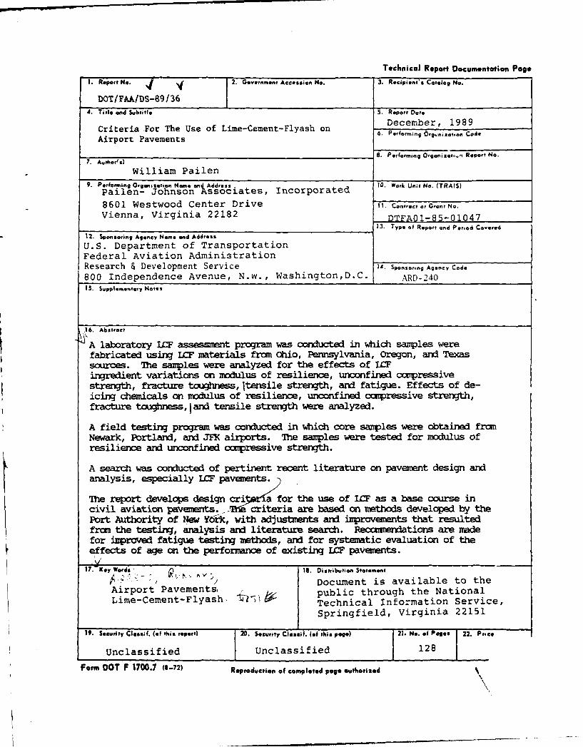
Criteria For The Use of Lime-Cement-Flyash on December, 1989

Airport Pavements Perforng Org.nmzatson Code

7._ 8, Performing Organizot,,m Report No.

7. A.,Aor'$)

William Pailen9. Performing Organization Name and Address 10. Work Unit No. (TRAIS)

Pailen- Johnson Associates, Incorporated

8601 Westwood Center Drive 11. Conrae, oGranNe.Vienna, Virginia 22182 DTFA01-85-01047

13. Type of Report and Period Covered

12. Sponsoring Agency Name and Address

U.S. Department of TransportationFederal Aviation AdministrationResearch & Development Service ). Sponsori.. Agency Code

800 Independence Avenue, N.w., Washington,D.C. ARD-24015. Supplementoy Notes

16. Abstract

A laboratory WCF assessment program was conducted in which samples werefabricated using LCF materials fran Ohio, Pennsylvania, Oregon, and Texassources. The samples were analyzed for the effects of LCFingredient variations on modulus of resilience, unconfined ccupressivestrength, fracture toughness, itensile strength, and fatigue. Effects of de-icing chemicals on modulus of resilience, unconfined ccupressive strength,fracture toughness, Iand tensile strength were analyzed.

A field testing program was conducted in which core sarples were obtained fromNewark, Portland, and JFK airports. The samples were tested for modulus ofresilience and unconfined cmpressive strength.

A search was conducted of pertinent recent literature on pavement design andanalysis, especially LCF pavements.

The report develops design cri or a for the use of ICF as a base course incivil aviation pavements. .. TWcriteria are based on methods developed by thePort Authority of New Yfrk, with adjustments and improvements that resultedfran the testing, analysis and literature search. Recouendations are madefor irproved fatigue testing methods, and for systematic evaluation of theeffects of age on the performance of existing ICF pavements.

17. Key Wod! 18. Distribution Statement

- Document is available to theAirport Pavements, public through the NationalLime-Cement-Flyash. Technical Information Service,

Springfield, Virginia 22151

19. Security Clesif. (of this report) 20. Security CIOssif. (of this peg.) 21. No. of Pages 22. Pric.

Unclassified Unclassified 128

Form DOT F 1700.7 (e-72) Reproduction of completed peg euthorized

This report resulted from a three year effort to accumlate and analyze

information on the performance of lime-cement-flyash (LCF) in airport

pavements and to develop criteria for the design of LCF pavements. The work

was performed under Federal Aviation Administration (FAA) contract number

DTFA01-85-01047. The FAA Technical Officer on this effort was Dr. Aston L.

McLaughlin, ADS-240. His guidance, assistance, advice, and critical review

were invaluable and are gratefully acknowledged.

Construction, testing, and analysis of laboratory samples were performed by

Resource International, Inc., in Columbus, Ohio under the leadership of V.R

Kumar, Director of Construction Services. Analysis of samples obtained in the

field was performed at Tuskegee University in Tuskegee, Alabama by graduate

student Subdoh C. Biswas under the guidance and direction of Dr. Shaik

Jeelani.

Accessi on For

NTIns GRA&IDTIC TABUnannounced 0

Distribution/

Availability Codes

Avail and/orDist Special

IDpi

0 ~om•m m m m mm mmmmm

TABLE OF COTENTS

1 Introduction and Background .................. 1

1.1 General . . . . . . . . . . . . . . . . . . . . . . . . . . . . 1

1.1.1 Introduction .......................... 1

1.1.2 Tehnical Background and Objectives ...... .............. 2

1.2 Current Paving Practices ........ .................... 5

1.3 Synopsis of Study Activities ........ .................. 6

2 Design and Conduct of Laboratory Tests ...... ............. 8

2.1 General ............ ............................ 8

2.2 Description of Materials Used ........ ................. 9

2.2.1 Lime ............. .............................. 9

2.2.2 Flyash ............. ........................... 9

2.2.3 Cement ............ ............................. 10

2.2.4 Water ............ ............................. 10

2.2.5 Sand ........... ............................. .. 11

2.3 Mix Optimization Concept ........ .................... 11

2.3.1 Previously Published Concepts ..... ................. .. 11

2.3.2 Proportions Used For Laboratory Tests .... ............. .. 13

2.4 Sample Preparation for Optimization of Mix ....... ...... 14

2.5 Test Results of Selected Mixtures ..... ............... ... 15

2.6 Optimized Mix Selection ....... .................... ... 32

2.7 Sample Preparation ....... ....................... ... 33

2.7.1 Cylindrical Specimens ....... ..................... .. 34

2.7.2 Beam Specimens. . ......... ......................... 35

iii

2.7.3 Aggregates ........................... 36

2.7.4 Speciren Construction ....... ..................... .. 38

2.8 Laboratory Tests ........ ........................ .40

2.8.1 Modulus of Resilience, Mr ........ ................... 40

2.8.2 Indirect Tensile Strength, sy ..... ................. .. 43

2.8.3 Fracture Tughess, Klc ..... ................... .... 43

2.8.4 Unconfined Cumpressive Strength, q .... ............... ... 44

2.8.5 Fatigue Tests ......... ......................... .. 45

3 Laboratory Test Results ......... .................... 47

3.1 General Results .......... ........................ 47

3.2 Unconfined Compressive Strength ..... ................ ... 70

3.3 Modulus of Resilience ....... ..................... .. 70

3.4 InKIirect Tensile Strength . ....... ................... 71

3.5 Fracture Toughness ....... ....................... ... 71

3.6 Effect of De-Icing Chemicals ...... .................. .. 71

3.7 Effect of Water pH Level ........ .................... 72

3.8 Fatigue ............ ............................ 72

3.8.1 Fatigue Test Results ........ ...................... .. 72

3.8.2 Suggestions for Additional Fatigue Tests ..... ............ 73

4 Design and Conduct of Field Tests ....... ............... 76

4.1 Objective ......... ........................... ... 76

4.2 Previous Research ....... ....................... ... 76

4.3 APprach .......... ............................ . 78

4.3.1 Ectraction of Cores ........ ...................... .. 78

iv

~Page

4.3.2 Testing of Extracted Cores ................... 93

4.4 Procedure for Irdirect Tension Test for ResilienceModulus of Elasticity ....... ..................... .. 93

4.5 Apparatus ........... ........................... 94

4.5.1 Testing Machine ......... ........................ .. 94

4.5.2 Deformation Measurements ........ .................... 94

4.5.3 Loading Strip ......... ......................... .. 94

4.5.4 Capping Equipments ....... ....................... ... 94

4.6 Procedure for Resilience Modulus Test .... ............. .. 95

4.7 Procedure for Unconfined Caipression Test ..... ........... 95

5 Field Test Results ....... ....................... ... 97

5.1 General Results .......... ........................ 97

5.2 Field Test Procedures ....... ..................... .104

5.3 Sample Calculation for Resilience Modulus for Core2A ........... ............................... 105

5.4 Sample Calculation for Unconfined Compression Testfor Core 2C .......... .......................... 105

6 Suggested LCF Pavement Design Guidelines ..... ............ 106

6.0 Approach ........... ............................ 106

6.1 Pavement Design Based on Control of Aircraft and PavementVibration Response ....... ....................... .108

6.2 Pavement Design Based on Elastic Mass Analysis ... ......... 110

6.3 Pavement Design Based on Stress, Strain and Strength

Relationships ......... ......................... 112

6.3.1 Pavement Design Based on Indirect Tensile Strength ......... .. 114

6.3.2 Pavecent Design Based on Compressive Strength ............ .115

v

6.4 Pavement Design Based on Fracture Tgess .......... 116

6.5 Margin of Safety ........................ 117

7 Recurmendations ........................ 118

Bibliography ......................... 119

vi

LIST OF TABLES

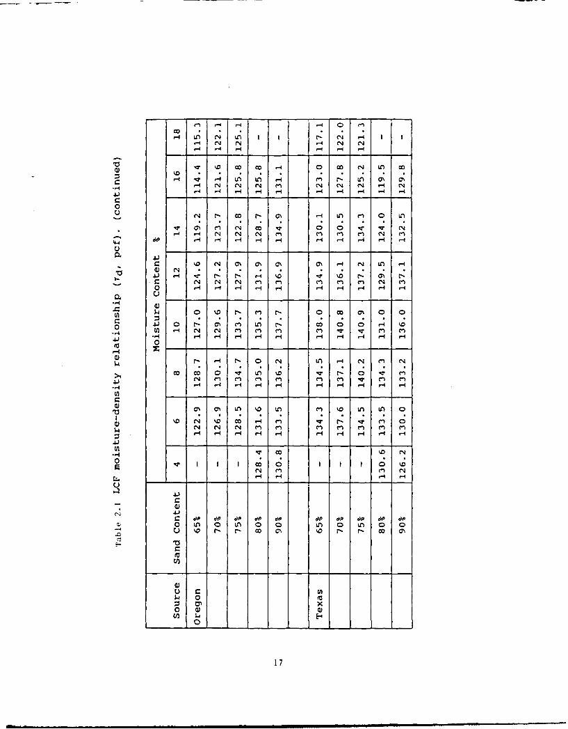
2.1 LCF Moisture-Density Relationship ...... ................ 16

2.2 Factorial Mix Design ........ ...................... .. 31

2.3 Aggregate Gradation Limits ...... ................... ... 37

2.4 Combined Aggregate Gradation of P-401 AsphalticConcrete ......... .......................... .. 37

2.5 Full Factorial Design of Experiment for LCF Mixtures ........ .. 41

2.6 Factorial Design of Experiment of LCF Mixtures ........... ... 42

3.1 Stmmary of Laboratory Test Results of Urea and Glycol DippedSamples. (Ohio Source) ....... .................... . 49

3.2 Summary of Laboratory Test Results. Ohio Source .... ........ 50

3.3 Summary of Laboratory Test Results. PennsylvaniaSource ......... ........................... .. 51

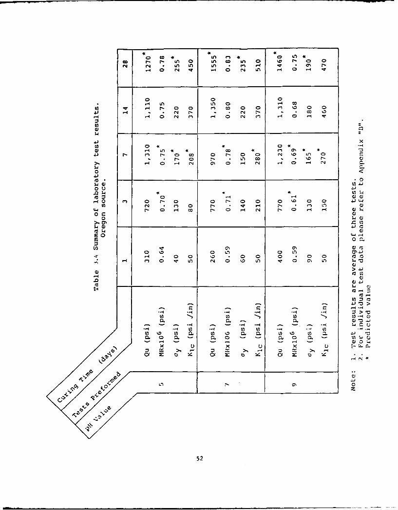
3.4 Sumary of laboratory Test Results. Oregon Source ......... ... 52

3.5 Summary of laboratory Test Results. Texas Source ... ....... 53

3.6 Fatigue and Flexural Test Results for LCF Specimens .......... 74

4.1 Portland Extraction Matrix ...... ................... ... 81

5.1 Compression Test Results ........ .................... 100

5.2 Compression Test (Field) Results vs Age of Pavement ......... .101

5.3 Modulus of Resilience . ....... ...................... 102

5.4 Resilience Modulus vs. Age of Pavement ..... ............ 103

vii

LIST OF FIGURES

Fi-Ire Pg

2.1 Moisture Density, Ohio ...................... 18

2.2 Moisture Density, Pennsylvania Source ...... ............... 19

2.3 Moisture Density, Oregon Source ..... .................. ... 20

2.4 Moisture Density, Texas Source. . ...... .................. 21

2.5 Sand Content Optimization ........ ..................... ... 22

2.6 Sand Content Optimization, Pennsylvania Source ............ ... 23

2.7 Sand Content Optimization, Oregon Source . .... ............. 24

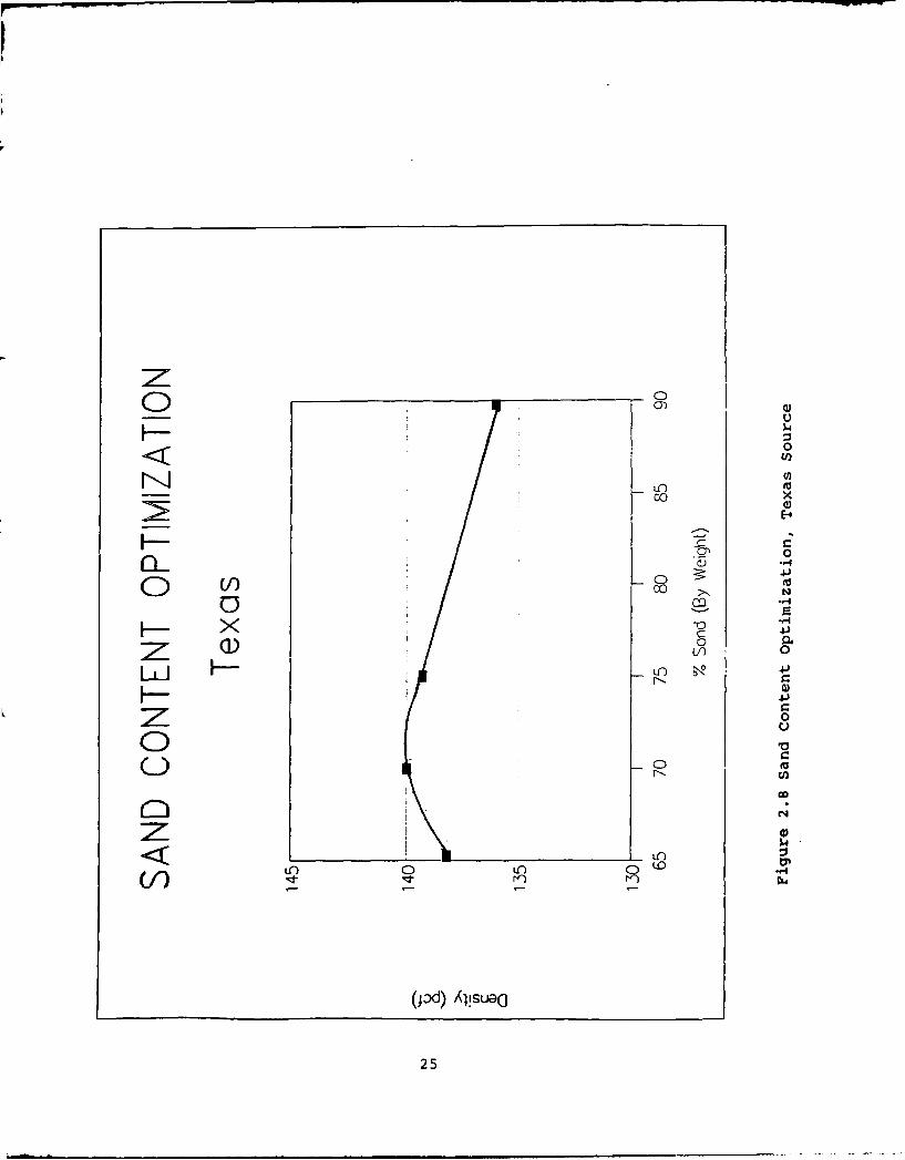
2.8 Sand Content Optimization, Texas Source ..... .............. 25

2.9 Moisture Density, Ohio Source ..... .................. ... 26

2.10 Moisture Density, Pennsylvania Source .... ............... ... 27

2.11 Moisture Density, Oregon Source ...... .................. .. 28

2.12 Moisture Delsity, Texas Source ...... .................. .. 29

2.13 Marshall Mix Design Data ..... .. ..................... ... 39

2.14 Fatigue Test Set-up .......... ........................ 46

3.1 Unconfined Compressive Strength vs. Time ... ............. .. 54

3.2 Unconfined Ccupressive Strength vs. Time ... ............. .. 55

3.3 Unconfined Ccmpressive Strength vs. Time ... ............. .. 56

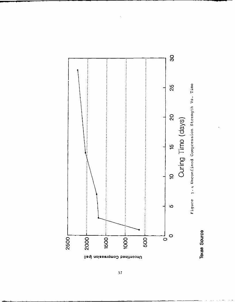
3.4 Unconfined Compressive Strength vs. Time .... ............. ... 57

3.5 Resilience Modulus vs. Time ...... .................... . 58

3.6 Resilience Modulus vs. Time ...... .................... . 59

3.7 Resilience Modulus vs. Time ....... .................... ... 60

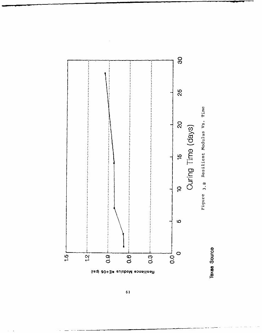
3.8 Resilience Modulus vs. Time ...... .. .................... 61

3.9 Indirect Tensile Strength vs. Time ..... ................ ... 62

viii

Fimire Bq

3.10 Indirect Tensile Strength vs. Time ................ 63

3.11 Indirect Tensile Strength vs. Time ....... ................ 64

3.12 Indirect Tensile Strength vs. Time ....... ................ 65

3.13 Fracture Toughness vs. Time ........ .................... 66

3.14 Fracture Toughness vs. Time ...... ................... ... 67

3.15 Fracture Toughness vs. Tire ...... .................... . 68

3.16 Fracture Toughness vs. Time ...... .................... ... 69

4.1 Effects of Curing Time and Temperature on the StrengthDevelopment of a Lime-Flyash-Aggregate Mixture ... .......... .. 77

A .2 Ccmpressive Strength Development of Lime-Flyash-StabilizedMixture in Chicago Area ......... ..................... 79

4.3 JFK Core Locations, 21 April 1986 ....... ................. 82

4.4 JFK Core Locations, 22 April 1986 ..... ................. ... 84

4.5 KMA Operational Plan ......... ....................... 85

4.6 Newark Core Locations, 23 April 1986 .... ............... .. 88

4.7 Newark Core Locations, 24 April 1986 .... ............... .. 89

4.8 Newark Core Locations, 24 April 1986 ...... ............... 9o

4.9 NIA Operational Plan ........ ....................... .. 91

5.1 Ccmpressive Test Results ....... ..................... .. 98

5.2 Resilience Modulus Test Results ...... .................. .. 99

ix

CHAPrER 1 - INTRODUCMION AND BACKGROUND

1.1 GEERAL

1.1.1 INRODUON

In recent years energy and environmental considerations have brought about anincreased interest in the use of ICF in pavement construction. A well-developed technology now exists for the stabilization of bases and subbaseswith these materials. However, ICF is not always used when it might beappropriate because technical information has not been conveniently available.The following factors are likely to influence the future use of LCF as a base

material for varied types of pavement construction:

o Increase in use of coal for fuel (i.e., increase in flyash supply),o Low energy requirements for producing ICF mixes,o New technology for LCF use, and

o Widespread availability of lime and flyash.

The primary factors affecting the performance of pavements with LCF baseand/or subbase 7 are:

o Loading,

o Interrelationships between load, pavement thickness, and material

strength,o Durability of the material as related to the environment it must

serve,

o Quality of Construction including uniformity of the final product,and

o Subsurface drainage of the pavement system.

Performance of pavement with I.F as a base/subbase has been studied by theFAA2 2 and others. 6,8,15,21,27,28 They have found that LCF base courses areviable materials for use in the construction of pavement. LCF has been usedwhen conventional materials or subgrades require stabilization. Because it cansometimes be purchased inexpensively, use of LCF may provide a basis for verycost-effective pavement construction.

1

Advantages of using ICF mixtures in pavement construction includes ease in

construction and the ability to use conventional construction equipment. The

essential requirements for use of LCF mixtures are thorough mixing, uniform

spreac-ag, and compaction to a high density.

Administrators, engineers, and researchers recognize the need for technical

information on the use of LCF as a base course material for pavement

construction. A well-developed laboratory methodology to determine the

effects of environment and external loading is an essential step in

establishing the physical and mechanical properties of ICF mixtures. These

properties could be used as an attempt to determine the short-term effects of

environment and external loading on LCF base course materials.

1.1.2 TECHNICAL BACKGRCUND AND OBJECTIV

The subgrade soil supports the pavement and the loads imposed on the pavement

surface. The pavement serves to distribute the imposed load to the subgrade

over an area greater than that of the tire contact area. The greater the

thickness of pavement, the greater the area over which the load on the

subgrade is distributed. Therefore, the more unstable the subgrade soil, the

greater the required area of load distribution and consequently the greater

the required thickness of pavement.

The soils having the best engineering characteristics encountered in the

grading and excavating operations should be incorporated in the upp r layers

of the subgrade if economically feasible. Because of these considerations,

soil conditions and the local prices of suitable construction materials are

the most important items affecting the cost of construction of landing areas

and pavements. 29

In certain locations of the country where airports are situated, native

materials for subgrade and/or base construction may be unsuitable. In view of

this, efforts are being made to stabilize the subgrade and base courses by

using cement, lime, and flyash in various ombinations with the existing

2

subgrade and/or base material. This recourse to construction of base and/or

subgr ad is being taken in view of the fact that it would be prohibitively

expensive to replace the unsuitable material by obtaining standard graded

material.

The use of lime, cement, and flyash in various combinations with the available

subgrade and/or base materials has helped to increase the bearing strength of

runways and taxiways used by heavy comercial aircraft. However it is not

known how the strength is effected on a long-term basis by ingress of

chemicals, rainwater, etc., and other environmental effects.

One purpose of this investigation is to develop a methodology to establish

material properties depending on optimal proportioning of lime, cement, and

flyash in different combinations, chemical activity, etc. Another purpose is

to study the long-term changes in the behavior of the combination of materials

that may occur as a result of pozzolanic activity and environmental forces.

Mix designs have been developed by the Port Authority of New York and New

Jersey2 5 for improvement of the base course using certain mixes of lime,

cement, and flyash. The design approach developed in this report follows that

of the Port Authority. But it also extends it by including stress/strain

characteristics of LCF mixtures from several regions of the United States, by

expanding the equations for prediction of maximum stress in a pavement slab,

and by providing some measurement data that may be helpful in assessing the

effects of aging.

The research included performing tests in the laboratory on trial mixes using

lime, cement, and flyash. The materials were obtained from four widely

dispersed geographic locations, and three water samples having different pH

values were used.

It is clear from literature and experience that LCF is a viable base course

material for airport pavements. However, the complex, long-duration nature of

the chemical reactions that occur within the mixture as well as the effect of

external loading, climatic and environmental conditions is . not well

3

understood, especially with regard to LCF pavement performance.

Destabilizing effects on lime and flyash due to chemical reactivity and lossof cementing properties are major factors in the performance characteristicsof the LCF mix. Measurement of physical and mechanical properties may provideinsight into short term effects, and distress function parameters may be used

as indicators for indicators for long-term effects.

By proper experimental design both short-term and long-term parameters willreflect not only chemical and cementing effects but also loading, temperature,

and environmental effects. 2 2

The objective of this study is to develop a design criteria and constructionprocedure for using ICF as a base course in civil aviation pavements.

Included in the scope of the effort is an evaluation of the mix designs andperformance characteristics of existing pavements as well as a laboratory

study to quantify the short and long term changes in material behavior as aresult of pozzolanic activity and enviromvental factors.

This report documents the activities and findings of Pailen-JohnsonAssociates, Inc. (PJA) and its subcontractors in conformance with the work

plan submitted to the FAA. The subcontractors are Resource International,Inc., in Ohio and Tuskegee University in Alabama.

4

1.2 CURRET PAVING PRACICES

Present FAA design practices for runways and taxiways consider two types of

pavements: (1) flexible, and (2) rigid. LCF however exhibits the

characteristics of a flexible pavement immediately after construction, and of

a rigid pavemnt as it matures. Hence, there is a need to develop a set of

design guidelines that is specific to IWF.

Flexible pavements consist of a bituminous wearing surface placed on a basecourse and, when required by subgrade conditions, a subbase. The entire

flexible pavement structure is ultimately supported by the subgrade.

The bituminous surface or wearing course must prevent the penetration ofsurface water, fuel or other solvents to the base course, provide a smooth,

well-bonded surface free from loose particles which might endanger aircraft or

personnel, resist the shearing stresses occasioned by aircraft loads, and

furnish a texture of nonskid qualities, without causing undue wear on tires.

The base course is the principal structural cauponent of the flexible

pavement. It has the function of distributing the imposed wheel load

pressures to the pavement foundation, the subbase and/or subgrade. The base

course must be of such quality and thickness to prevent failure in the

subgrade, withstand the stresses produced in the base itself, resist vertical

pressures tending to produce consolidation and resulting in distortion of thesurface course, and resist volume changes caused by fluctuations in its

moisture content.

Rigid pavements for airports are composed of portland cement concrete placed

on a granular or treated subbase course that rests on a compacted subgrade.Under certain conditions of soil classification, drainage and frost, a subbase

is not required.

The concrete surface must provide an acceptable nonskid surface, prevent the

infiltration of surface water, and provide structural support to the aircraft.

5

The use of ICF in highway and selected aviation pavements has been an accepted

practice for over 20 years. In many instances the long term strength gain of

these pavements has exceeded the initial design goals of the projects. Little

data has existed, however, on the effects of environmental situations such as

the ingress of chemicals with rainwater on the pavement. In the aviation

environment, these problems have been further cxmplicated by the lack of

design guidelines directly applicable to ICF.

1. 3 SYNOPSIS OF SIUDY ACIVITIS

The approach used in developing the specification results from the following

activities:

o A search for pertinent recent literature on pavement design and

analysis, especially ICF pavements,

o Conduct of a laboratory LCF assessment program in which samples were

fabricated using LCF materials from four areas and were analyzed for

the effects of LCF ingredient variations on modulus of resilience,

unconfined ccapressive strength, fracture toughness, tensile

strength, and fatigue, and

o Conduct of a field testing program in which core samples were

obtained frum four airports and were analyzed for the effects ofpavement age on modulus of resilience and unconfined compressive

strength.

0 Adaptation of design methods developed by the Port Authority of New

York with adjustments and improvements that resulted from the

testing, analysis and literature search. The following adjustments

and improvements were made:

LCF stregth cracteristics that resulted from the tests are

available for preliminary design and planning.

6

Equations for calculation of the maximum tensile and

ccapressive stresses imposed by an aircraft load on a pavement

slab are exparded to take into account the location of the load

relative to the edges of the pavement.

7

CHAPTER 2 - DESIGN AND CNEILJCT OF IABORATORY TESTS

2.1 L

The purpose of the laboratory test activities was to investigate short-term

and long-term nroperties of LCF as they are affected by pozzolanic activity,

environmental forces, chemical activity, and optimal proportions of

ingredients. From the investigation a database of information was acquired toserve as a baseline to develop a design methodology and construction procedure

for the use of LCF as a base course.

The work effort was divided into two parts, sample preparation and sampletesting. Two factorial designs were used in sample preparation. The full

factored design varied four (4) mixes (varying proportions of LCF sand), three(3) pH values (basic, normal, acidic), and five (5) ages for a total of 60different combinations. The smaller design varied three (3) ages (varying

maturity), three (3) pH levels (acidic, normal, basic), and two (2) de-icing

chemicals (urea and glycol) for a total of eighteen (18) different

combinations.

The investigation of LCF mix designs which meet FAA design requirements was

performed to resolve the following questions for four different LCF sources.

o What are the effects of aging on the mechanical properties and

performance of the mix?o What are the effects of mixing water pH on the mechanical properties

and performance of the mix?o What are the effects of occasional exposure to de-icing chemical?

8

2.2 DERIPTION OF MALTERIALS USED

Four sources for LCF materials were investigated. They were Ohio,

Pennsylvania, Oregon and Texas. Cement, sand, and water were procured from

Ohio, while lime and flyash were procured frao the four sources suggested

above. The physical properties of the material were to conform to the

specifications detailed below:

2.2.1 LIM

In general the term lime refers to oxides and hydroxides of calcium and

magnesium, but not to carbonates. There are various types of lime ccamercially

available. The type of lime used in this research study was Type N, and

obtained from four different sources/regions, as stated earlier.

2.2.2. AS

Flyash is the finely divided residue that results fran the combustion of

ground or powdered coal and is transported from the boiler by flue gases.

Flyash is collected from the flue gases by either mechanical or electrostatic

precipitation devices.7

Flyash is a pozzolan and is defined as "a siliceous or siliceous and aluminous

material, which in itself possesses little or no cementious value but which,

in finely divided form and in the presence of moisture, reacts chemically with

calcium hydroxide at ordinary taqperatures to form ccmpourds possessing

cementious properties."22

Flyash is available in different conditions. "Dry" flyash is taken directly

frcm the precipitator or from dry storage. If the flyash is stockpiled in the

open at--kpere, it is normally conditioned by adding water to prevent

dusting. Some conditioned stockpiled flyashes may develop cementious

properties and "set up" in the stockpile. If the flyash has set up, crushing

and screening may be required prior to use in stabilized mixtures. In some

9

instances the collected flyash is slurried into storage pond areas and must

subsequently be reclaimed frcm the pond for use.7

Typical ranges of values for the chemical cwposition of flyash are:

Principal Constituents

Si02 28-52A1203 15-34

Fe203 3-26

Cao 1-10

M90 0-2

S03 0-4

Loss on Ignition 1-30

2.2.3

The type of cement used in this study was Type I Portland Cement conforming to

ASTM C150.

2.2.4 ATER

The type of water used in this study was potable water from city water supplysystem with a pH value of 7. As sanples of ICF were to be tested fordetermination of the effect of pH value, "pH down" chemical manufactured byAquarium Pharmaceuticals was used to bring the pH value of water to 5 (makewater acidic) and lime was added to water to bring the pH value to 9 (makewater basic). Lime from the four sources was used to make the water basic forpreparation of respective samples.

10

2.2.5

The type of sand used was natural sand obtained from river sources, with not

more than 10 percent by weight passing the #200 sieve. The other material

properties of sand are listed below:

o Sieve analysis

Sieve Size Percent Passinq

#4 100

#8 97.5

#50 28.9

#100 8.6

#200 4.8

o Soundness - 6.4 percent.

According to FAA aggregate gradation requirements, a wide range of gradations

is permitted for base course construction. FAA also permits the use of clear

sand and if a substantial portion passes sieve #4, the combined LCF gradation

is to be adjusted to produce the maximum dry density in the compacted mixture.

2.3 MIX OPIIZATION CONCEP'

2.3.1 PREVIOUSLY UBLUSHED CONCEPIS

Review of published literature revealed much detailed information on mixture

properties of lime-flyash-aggregate (LFA) mixtures and the factors which

influence these properties. Although LFA mixtures do not contain cement,

which is added to acoelerate hardening, analysis of their properties gave some

insight into the performance range of lime-cmwt-flyash-aggregate (LCFA)

properties.

11

Initially, the early strength properties of LCF mixtures may be higher than

those of LFA due to the effect of cement, but over the course of time the LFA

strength properties approach the strength properties of LCF mixtures due to

continued pozzolanic activity. It was noted that the factors having the

greatest influence on LFA mixtures are: 1

o Proportions,

o Materials,

o Processing, and

o Curing.

A review of the methods used to proportion the total quantity of lime plus

flyash and the lime to flyash ratio has not produced a clear answer for the

best procedure. It is generally agreed that lime-flyash stabilization is best

suited for sands and gravels; and that the quantity of lime-flyash to be added

depends upon the gradation of the soil. Some investigators feel that lime and

flyash should be added to produce the maximum density mixture, others feel

that the best mixture is a function of water content.

The gradation of the soil is the major contributor in determining the total

amount of lime plus flyash that is added to the material. The objective is to

add enough lime and flyash to the mixture to be able to form a dense mass when

campacted. It has been shown, that the ability of a soil to carry loads is

related to soil gradation. 3 Narrowing the band of particle size tends to

reduce the load carrying capacity of the soil. Hence, the addition of LFA to

a poorly graded soil acoomplishes two things; the pozzolans react with lime to

form a cementious compound, secondly it produces a better graded mixture with

improved load carrying capacity.

Flyash reactivity and the amount of fines present in a soil are two important

characteristics affecting the ratio of line to flyash. Reactivity has been

shown to be directly related to the fineness of the flyash. 8 Viskochil4

investigated this relationship and concluded that 1:9 or 2:8 were the optimal

ratios for lime to flyash for sand, silt or clayey soils when 25 percent

flyash was used. Other investigators 5 have developed different ratios with

12

the most common being 1:3 and 1:4. Viskochil and Hoover 4 concluded that

greater compaction and corresponding high densities result in higher strengths

regardless of the lime-flyash ratio. Hollen and Marks 6 went further and

suggested a method for determining optimal mixture based upon obtaining the

greatest density.

The optimal mixture is frequently referred to as that which produces the

greatest density. However, a study done by the Corps of Engineers 5 in 1976 on

sandy gravel-lime-flyash and clay gravel-lime-flyash mixtures concluded that

the maximum density did not produce the greatest strength. They concluded

that strength was dominated by water content, with the highest strengths

occurring at 1 to 2 percentage points dry of optimum.

It has been suggested that the optimmal lime to flyash ratio is generally

dependent upon the material being stabilized and the reactivity of the flyash.

Due to the variability of aggregate and flyash properties, it is very

difficult to project optimal lime to flyash ratios without the actual testing

of several specimens over a range of IFA proportions.

2.3.2 PROPORTIONS USED FOR LABORAT1ORY TESTS

Proportioning of lime, cement, flyash, and sand was to be made so that the

final selected mixture can be used for the designated purpose. For this

study, the bases for proportioning the material components by weight were as

follows:

" For Ohio, Texas and Oregon sources of lime and flyash, the lime

content was to be between 2.5 and 4.0 percent, flyash content from

11 to 15 percent, lime to cement ratio to be kept below 3:1 and the

sand content to be varied as necessary. These proportioning

standards were to be used to determine the final LCF proportions.

o For the Pennsylvania source of lime and flyash, the chosen mix

proportions 3.2 percent lime, 0.8 percent cement, 13 percent flyash,

and 83 percent sand.

13

For the Ohio, Texas and Oregon sources, the percent factors that can be varied

in the mixture selection process are the amount of lime, flyash, and cement,

but within the guidelines set above, and varying sand content as required.

The job mix formula was determined by laboratory mix design procedures, which

included selecting the final mix proportion based on: (i) moisture-density

relationship and lime + flyash ratio for selection of sand content, and (ii)maxim unconfined compressive strength obtained from a laboratory-developed

curve for unconfined compressive strength and lime + flyash ratio.

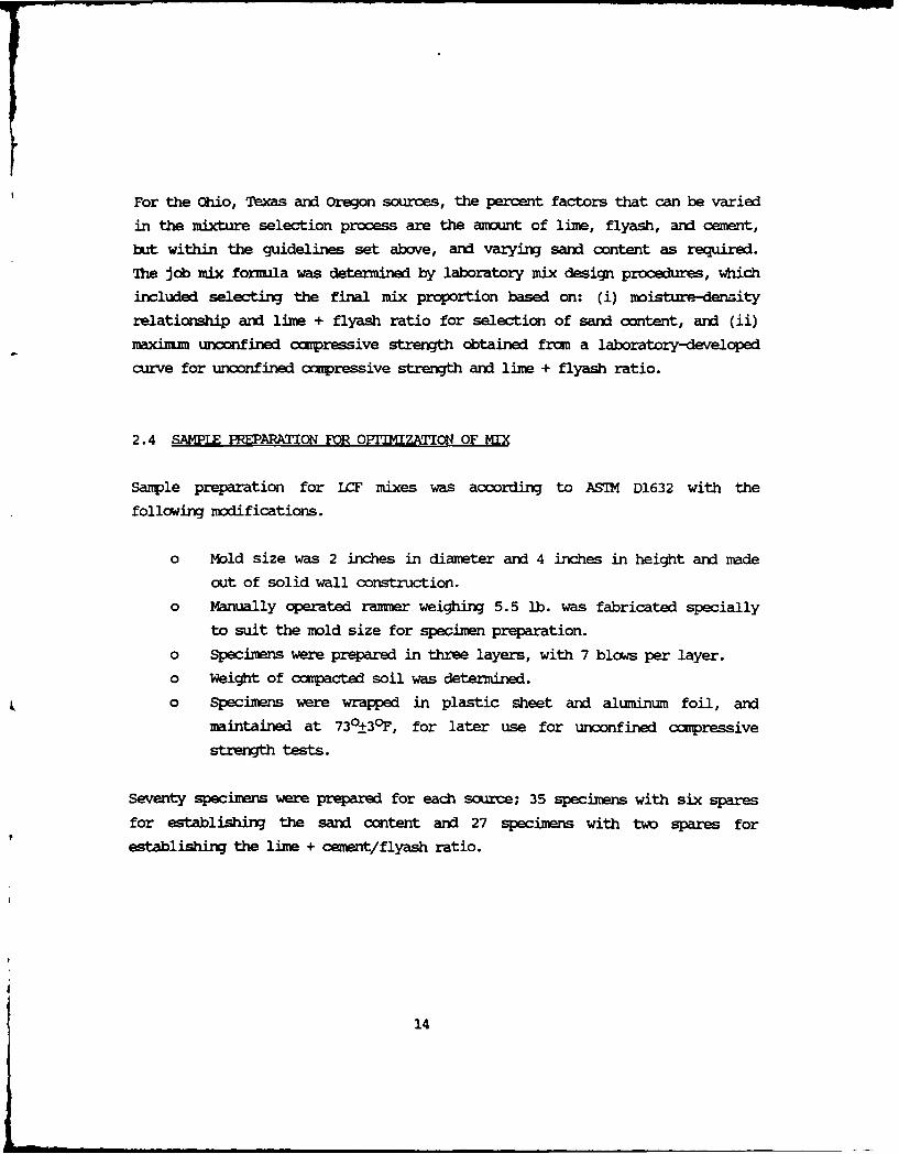
2.4 SAMPLE PREPARATION FOR OPlIIZATION OF MIX

Sample preparation for LCF mixes was according to ASIM D1632 with the

follwoing modifications.

o mold size was 2 inches in diameter and 4 inches in height and made

out of solid wall construction.

o Manually operated rammer weighing 5.5 lb. was fabricated specially

to suit the mold size for specimen preparation.

o Specimens were prepared in three layers, with 7 blows per layer.

o Weight of compacted soil was determined.

o Specimens were wrapped in plastic sheet and aluminum foil, and

maintained at 73°+30 F, for later use for unconfined compressive

strength tests.

Seventy specimens were prepared for each source; 35 specimens with six spares

for establishing the sand content and 27 specimens with two spares for

establishing the lime + cement/flyash ratio.

14

2.5 TEST RESUL OF SELECTED

Mix proportions for sand content optimization were designed as detailed below.

Case Cement Lim Flyash Sand

i 2.25 6.5 26.25 65

ii 1.9 5.6 22.50 70

iii 1.6 4.70 18.70 75

iv 1.25 3.75 15.00 80

v 0.625 1.875 7.50 90

For the moisture-density relationship, samples were fabricated with a water

content range of 4 percent to 18 percent at increments of 2 percent. Test

results are presented in Figures 2.1, 2.2, 2.3, and 2.4. For sand-content

optimization, samples were fabricated with a sand content range of 65 percent

to 90 percent. Test results are presented in Figures 2.5, 2.6, 2.7 and 2.8.

For sand content optimization at optimal moisture and dry density a total of

35 samples per source were tested and results are tabulated in Table 2.1 and

graphically presented in Figures 2.9, 2.10, 2.11, and 2.12. Test results are

sLunrarized as follows:

Maximum IrCF Density, pcf, for Different Sand Contents

Sand Content % by weiczht)

65 70 75 80 90

Ohio 127 131 133 136 134

Pennsylvania 129 131.5 135 137 133

Oregon 128.5 130 135 135 137

Texas 138 140 139 137.5 133.5

15

N4 -4 LO 0 l

.4 N N CN CN rr4 -4 -q -4 4 f-4

N Cl -9 U, N

1-4 0 N U, U)-4 N LC) 0N N N N N N N N en r)

r4 r- r 4 ,4q - H -4 .4

4-4

14 (1 N c , 3

4) Ln N co r-4 en' 0C N NV N m r) N m Nl M I-)

0 -4 4 H4 H4 H4 e 4 H- .- 4 H

4)

4) N UUj) P U, N 0N N m l '3

CN N rn en Ml Nq Nl enCl04 r~-4 14 H 1-4 H H H

CC )

Cf H N l Cl Cl C N N NlCl C-- 4 H -4 H H H H4

0

4-4

0 C 3~U0 ~i:

'3 H Cl N 0~ ~ 0 ~ C N6

1-4 LO (N U, I IN (N - Ir4 ( (N 4 (N (N

-4 4 -4 1 - -4 'I 4

V k0 .0 0 -0 0 (N LO 0o

1- N NN03C1 - 1

0'u- r. co U, , .-% -4 N) C 0 V)

1- 4 el N (N (N m (n (n (n m4 (do) -4 r-4 -4 -4 -4 f-4 -4 -4 -4 1-4

4)

-4~c m.. (Nn N ClC l C (N4 M0s r.

4 .4 -4 .-- 4 4q r- 4 r-4 q 1-

4-)(o 0N 0 ' 0 ' - N U -

4-) e4 co N N '0 %D0 f ' n4.)N ell en (n ml Ml ml e N

0A -4 4 -4 H4 -4 -4 -4 -H4 -

0N '.% It Cl N 0) 0 0

JJ 0 N %D co r-4 N) v 0, 0 4-

v-I m 4 vI H 4 H -H-4 f-4 M4 v-I H

4.)

0N ~ - H- H NU -I ( l (

0 ti0 0 0 V) 0 N l 0 0 C%D r, r, co C\ Cl r, r, co a\

030

I U *

0 0 tv(

00

I I 0 I I 17

0

LU (D

00

LUj

I 00

CD3

mON

cli

0o to 0

01d)169M u ACj %

18

co

C.)

UI) U.i

Lu.4-J

-C:

- 0

a)) C

.4-1Q

0

1-4

I 0m

0 LO 0 LO 01qcocoN N~

(Jod) iL6eMfun ,UC

19

* cc

0

Cl) * * * U

0

CPC

0 0

clii

0 c *l coED0

Cl)d lqi*~u ~ (

20'-

* U

(1) 0

LU EA

COn

LUQco o

LO *O 0 D

19. Clo U, NC

C')d ico iu A(

210

0

0

F 4J

o £ --- ("(,**) --4' -

- - ~ J-0

p K- -

K) a)

22.

-4

0

c~u

/23

7F 0

U- 0 n

244-

o G)0

0

co x

F- 0

(I)Co 4J

F- -_c4.0Lo 0

F---0

00

U-U

rn2

(pod) Al!sua(0

25

C'.'

* 0

* co

00

LO 0

wU q

0 -10 0

Li

0

0 01(I),

o LOb 44

0

c) zb LIH

COco z0~z* . . x

(=10) AIN3C AU

26

____ ____ ___ ____ ___ to

o U)c."Ej

0 40

-~ 0.

H ~J)0*': 0

co m z

opc~

00

LO to zot

(00d) A.LISN3G AUG 0'

27

LO

L cii

c60

0

LUHC

0 C:

/o 0cc~(C 0* )F-. o

C6co,0 k

cooc zl

(00d) AIISNHG AUG

28

C~CD

* .0

U)

LU

*00

to 0

0C3

LO LO LOLO -j

(=10d) AIISN3G AUG

29

The results of this table and Figures 2.9 through 2.12 illustrate the sand

content optimization for Ohio, Pennsylvania, Oregon, and Texas sources,respectively. These curves result in the following optimal sand contents:

Sand Moisture Maximum

Content Content Density

(%) (%) (pcf)Ohio 80 10 136

Pennsylvania 80 10.5 137

Oregon 80 9 135

Texas 73 10 140

Mix proportions for optimization of lime, cement, flyash ratio were designed

as detailed below:

Design of experiment according to Table 2.2, 'ix Design Factorial" wasconducted for four sources: Ohio, Pennsylvania, Oregon and Texas. Nine mix

combinations for each source were proportioned as summarized below:

Mix proportions for cement, lire, and flyash optimization

Mix Combination Cement Lime Flyash Sand

(Lime: Flyash)

2.5 : 11 .7 2 11.7 85.6

2.5 : 13.5 .65 1.95 14.0 83.4

2.5 : 15 .64 1.92 15.4 82.0

3.25 : 11 .86 2.59 11.7 84.9

3.25 : 13.5 0.84 2.52 14.0 82.7

3.25 : 15 0.83 2.48 15.3 81.4

4 : 11 1.05 3.15 11.6 84.2

4 : 13.5 1.03 3.07 13.8 82.0

4 : 15 1.01 3.03 15.2 80.8

30

Table 2.2 Factorial Mix Design

4 253.25 4

x X x

OHIO 13.5 x x x

15 x X x

12. x x X

OREGON 13.5 x X x

15 x X

11 x X x

TEXAS 13.5 x x x

ft 115 x x x

Line/Cement Ratio 3 :1

Sand Content V.ariable according to the above proportions.

3 replicates

31

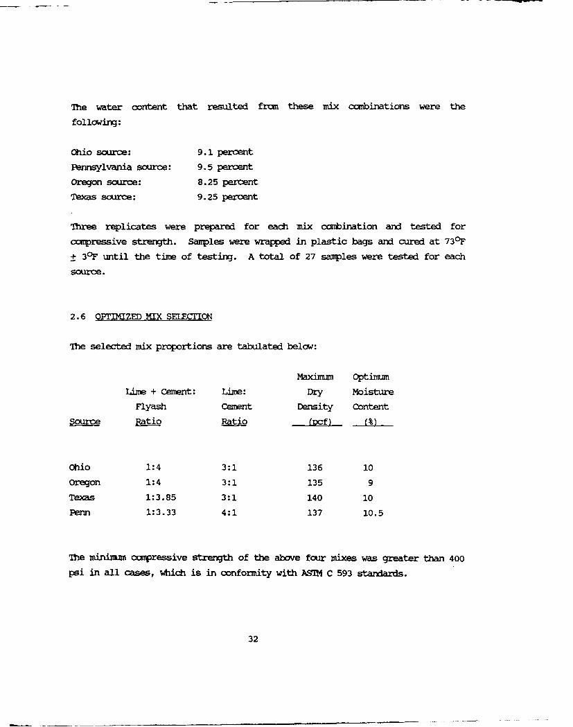
The water content that resulted from these mix combinations were thefollowing:

Ohio source: 9.1 percent

Pennsylvania source: 9.5 percent

Oregon source: 8.25 percent

Texas source: 9.25 percent

Three replicates were prepared for each mix combination and tested for

ocmpressive strength. Samples were wrapped in plastic bags and cured at 730 F

+ 30F until the time of testing. A total of 27 samples were tested for each

source.

2.6 OPTIMIZED MIX SELECTION

The selected mix proportions are tabulated below:

maximum Optimm

Lime + Cement: Lime: Dry Moisture

Flyash Cement Density Content

Source Ratio Ratio 1cf). LM

Ohio 1:4 3:1 136 10Oregon 1:4 3:1 135 9

Texas 1:3.85 3:1 140 10Penn 1:3.33 4:1 137 10.5

The minimum cxmpressive strength of the above four mixes was greater than 400

psi in all cases, which is in conformity with ASIM C 593 standards.

32

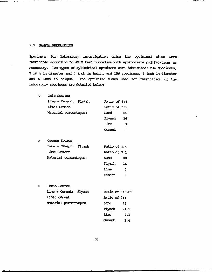
2.7 SAMPLE PREPARATION

Specimens for laboratory investigation using the optimized mixes werefabricated according to ASIM test procedure with appropriate modifications asnecessary. Two types of cylindrical specimens were fabricated: 234 specimens,2 inch in diameter and 4 inch in height and 156 specimens, 3 inch in diameterand 6 inch in height. The optimized mixes used for fabrication of thelaboratory specimens are detailed below:

" Ohio Source:

Lime + Cement: Flyash Ratio of 1:4

Lime: Cement Ratio of 3:1

Material percentages: Sand 80

Flyash 16

Lime 3

Cement 1

o Oregon SourceLime + Cement: Flyash Ratio of 1:4

Lime: Cement Ratio of 3:1

Material percentages: Sand 80

Flyash 16

Lime 3

Cement 1

o Texas Source

Lime + Cement: Flyash Ratio of 1:3.85

Lime: Cement Ratio of 3:1

Material percentages: Sand 73

Flyash 21.5

Lime 4.1

Cement 1.4

33

o Pennsylvania Source

Lime + Cement: Flyash Ratio of 1:3.33

Lime: Cement Ratio of 4:1

Material percentages: Sand 83

Flyash 13

Lime 3.2

Cement 0.8

Sand was oven-dried before use in the mix. Proportioning of all ingredients

in the mix was by weight, except water which was by volume. The quantity of

water used in the mix for various sources is indicated below:

Source Specimen Size (in.) Water in CC. per Specimen

Ohio 2 x 4 50

3 x 6 160

Oregon 2 x 4 45

3 x 6 144

Texas 2 x4 50

3 x 6 160

Pennsylvania 2 x 4 52.5

3 x 6 168

2.7.1 CYLUMCAL SPECIMS

Water in measured quantities was added to the solid cuponents of the mix and

mixed in a mechanical mixer until the mix was homogereous. Specimens of size

2 in. x 4 in. and 3 in. x 6 in. were prepared by crpacting the mixed material

in the 2 inch and 3 inch molds respectively with collars attached. The

ccnpaction was performed in three 3 approximately equal layers to give a total

cumpacted depth about 5 inches and 7 inches respectively for the two specimen

sizes. Each layer was compacted with 7 uniformly distributed blows from the

34

5.5 lb. sleeve-type rawer dropping free fron a height of 12 inches above the

elevation of soil. During compaction, the mold rested on a dense, firm,

uniform, and stable base. Following ompaction, the extension collar was

removed and the cumpacted soil was trimmed flush using a straightedge. The

mold and moist mix were weighed and recorded. The mold with the moist mix was

then wrapped with plastic and aluminum foil and oven-dried for 24 hours at 140

OF. The specimen was extruded from the mold after 24 hours of oven-drying,

and weight of specimen determined, wrapped in plastic and aluminum foil, andkept in oven again at 140°F to await test. The dry density and moisture

contents of the mix were determined for comparison with the optimized mix

design data established earlier.

Specimens of size 2 inch x 4 inch were used for unconfined compressivestrength tests. Specimens of size 3 inch x 6 inch were saw-cut after removal

from molds into three approximately equal sections of 3 inch x 2 inch, andused for modulus of resilience, indirect tensile strength, and fracture

toughness tests. Separate sets of samples were prepared for the three pH

levels of water.

To determine the effect of de-icing chemicals on the material properties of

LCF mix, the specimens were dipped in urea and glycol and tested for the same

properties as for the control specimens. In order to minimize the cost of the

study, these tests were performed only on the Ohio source material. The

specimens were dipped in glycol/urea for 24 hours before the tests.

2.7.2 BEAM SP S

In addition to cylindrical specimens, composite beam specimens were fabricated

for fatigue and reflection cracking tests. The sizes and number of beam

specimens fabricated are detailed below:

35

Ohio Source: LCF base thicknesses of 2 inch, 3 inch, and 4 inch.

Asphalt concrete overlay thicknesses of 1 inch, 1-1/2 inch, and

2 inch.

18 specimens to be tested at two stress levels.

Similar specimens were fabricated for the other three sources of materials.

The asphalt concrete mixtures used in the preparation of fatigue specimens

were selected to meet the FAA specifications for asphalt concrete wearing

course.

2.7.3

Crushed limestone aggregate from a local American Aggregate Caqpany wasutilized for the manufacture of asphalt concrete specimens. The aggregates

used were #57 crushed limestone as the coarse aggregate and natural sand asthe fine aggregate. The crushed aggregate generally showed sharp, angular,

and gritty particles and, for the most part, contained at least one fractured

face in the particles and were reasonably free from excessive dust or other

deleterious coatings, weathered pieces, or excessive flaky and/or elongatedpieces. Measured water absorption of particle size ranged between 2.9 percent

and 3.2 percent. Aggregate gradation conformed to FAA specifications forasphalt concrete surface course. Gradation ranges of the #57 crushedaggregate and natural sand, based on frequent samplings, are shown in Table

2.3. Table 2.4 gives details about the combined gradation of #57 limestoneaggregate and natural sand used in the developnent of the P-401 mix. Design

of aggregate blends for this investigation is based or:

(i) Raw material aggregates and their individual gradings.(ii) General conformance with FAA specifications for P-401 mix.

For mix design and investigation, five proportions of aggregate were used:

5.5, 6, 6.5, 7, and 7.5 percent by weight of total mix.

36

Table 2.3

Aggregate Gradation Limits

#57 Lime Stone Natural Sand

Sieve Size % Passing Sieve Size % Passing

1/2" 100 3/8" 100l" 95-100 #4 95-100

1/2" 25-60 #8 70-100W 4 0-10 #16 45-80#8 0-5 #30 25-60

#50 5-30#100 1-10#200 0-4

Table 2.4

Combine Aggregate Gradation of P-401 Asphaltic Concrete

Sieve PercentSize Passing FAA Gradation Limits

1/2" 100 1003/8" 91 79-93#4 70 59-73#8 58 46-60#16 45 34-48#30 30 24-38#50 17 15-27#100 9 8-18#200 3 3-6

Note: 1 in. = 25.4mm

37

2.7.4 SPECIMEN CONSTRUCTION

The optimal asphalt content for the selected aggregate gradation was

determined using Marshall design procedures and 75 blows/face compaction

efforts. Optimal asphalt content was determined as the average of asphalt

content for optimum stability, density, and 4 percent air voids. Figure 2.13

shows the Marshall mix design properties for this mix.

Specimens were constructed in two stages. First asphalt concrete beams 3 inch

wide, 24 inch long and three thicknesses namely 1 inch, 1-1/2 inch, and 2 inch

were fabricated. This included an asphalt concrete hot mix which was prepared

in the laboratory and placed in a steel beam mold according to the job-mix

formula referred to above. The temperature of the mix was about 280 0F. A

wire comb was passed through the loose hot mix back and forth for even

distribution of the mixture in the mold. The mixture in the mold was then

pressed under steadily increasing load until the asphaltic mixture was

compacted to a desired thickness rather than specific load to ensure that

desired density would be achieved. The mold was then dismantled and the

specimen was placed on a stiff support, such as a piece of wood or steel, to

await the second stage of specimen preparation. All precautions were taken to

prevent damage to the beam samples before the next stage of specimen

preparation. The compacted specimens were allowed to cool at roan temperature

for 24 hours.

The second stage of specimen preparation consisted of joining the WCF mix with

the asphalt concrete beam. The asphalt concrete beam was treated with a prime

coat of MC-70 cutback asphalt at the rate of 0.25 gallon per square yard (1.1

liter per square meter) and allowed to cure. The beam was then placed in the

steel mold and LCF mix of predetermined quantity was placed over the asphalt

concrete beam. A wire oamb was passed through the loose mix back and forth

for even distribution of the WCF material over the asphalt beam. The mixture

in the mold was cumpressed uniformly with increasing load until the LCF

mixture was ompacted to the desired thickness to ensure that desired density

would be achieved. The maximm load was then maintained constant for 2 to 3

38

Marshall Mix Design

2400.. . .... .... ...... .

2300 -- 12 ...... X . ...

S2200 .... .. to. . . .. .

0 . . . . . . . . . . . . . . . . .... . .. . .

2100 .. . .. . .. . . .

2000 .. 6.. .

5 5.5 6 6. 5. 6 ~5 7

%. AC by Wt. of Mix. AC by WI of 161.

5 . ................................ ....... I

0 :............... ....... ..............

2 ....

K. AC. : o i : AC by W . f

16 . .

.. . .. . .. . . .... e -

5 565 6 6.5 75 55 6 5 7

% AC by W1. of Mi. AC by Wt. of Vi.

Fgr.13. Mashal.mx.dsig.daa.fr...0

17 ...... ..... ..... ..... ... .... ... ..3. ...

minutes until the pressure was stabilized. This procedure enabled the same

optimal density of the LcF, as was determined by mix optimization to be

obtained. The mold was then dismantled and the specimen placed on a stiff

support, such as wood or steel plate. The specimen was wrapped with plastic

and aluminim foil and cured at room temperature of 73 OF + 3 F for 60 days.

2.8 IAORATORY TESTS

The specimens prepared according to the procedures delineated in section 2.1

were tested to establish the following properties:

o Modulus of resilience,

o Indirect tensile strength,

o Fracture toughness,

o Unconfined compression, and

o Fatigue.

A full factorial design format for the laboratory tests for mixture

characterization is presented in Tables 2.5 and 2.6. The procedure for

conducting each type of laboratory test is described in the following

subsections.

2.8.1 MODWS OF RESILIENCE. Mr

The concept of diametrical (resilience) modulus has been previously applied to

asphaltic mixtures. For short-duration dynamic loads, the value for Young's

Modulus (E) is similar to the value for Resilience Modulus (Mr), a material

property useful in pavement analysis. The test required to determine Mr

involves applying a dynamic load of known duration and magnitude (below the

indirect tensile strength of the sample) across the vertical diameter of the

cored specimen. The elastic deformation across the horizontal diameter of the

specimen is measured with displacement transducers. After recording the

40

4

x

0%

0

(a 0 . 4 C - 0

E-4

0- en - '• - ~-. -:to"

0

0 0" (-n 0nW M

0 0 • U .

00

0) Cl Cl Cl (C) 44

4 r. :3o -4c '.1 c0 0 o a- '-.4

0 0 -4 Z 04-4

o~~~~4 0i C l lHJ l01

Ir -44t

0 0 c u-O) 0

-'4 Q4-*

1-4 4

U) 41 0 (

E-4U ~

C--I 0

0 fn (

'0;

44

0~ O1 -)~ U C$-4 -4 it :)

00q) 0

4) & r4-J X 0o. 0 U 0 0- CD M Lf (n 14.4 -

HX ' , '0

0 w c 0 0

N . .- 4 0 r- ,-

41 aCL x 41a 0

X ..- j w ,--

0 E

2.4 41

14~-4 4-2~fu

-4

00

42.

magnitude of the dynamic load and deformation, the Modulus of Resilience (Mr)

is calculated using the equation:

P(u + 0.2734)Mr= (2.1)

dt

where:

P = Magnitude of dynamic load;

u = Poisson's ratio

t = Specimen thickness

d = Total deformation

2.8.2 INDIRECT TENSILE SIRENGH,.Sy

The ultimate strength of an asphaltic mixture under an indirect tensile stress

field is obtained after diametrically applying a vertical load, at a rate of

load piston increase of 0.065 inch/minute until the maximum load (yield

strength) that the specimen is able to withstand, is reached. The indirect

tensile strength (Sy) is then calculated using the equation:

2PSy= (2.2)

3.14Dt

where:

P = Maximum load, (lb.)

D = Specimen diameter, (in.)

t = Specimen thickness, (in.)

2.8.3 FRA. 2I- ESS. KIc

The Ohio State University procedure was used to determine the fracture

toughness (Klc) of cored specimens. The method consists of cutting a right-

angled wedge into the core specimen and initiating a crack (0.25 in. long) at

the top of the notch. The specimen is set on a base with the wedge pointing

upwards, and a vertical load is applied to it through a three-piece set up

43

consisting of two plates (placed against the sides of the wedge) and a

semicircular rod placed between the two plates to transmit the load to the

sides of the wedges.

The results of the tests (conducted at roan temperature) allowed the

calculation of the fracture toughness, Kic through the equation:

PKlc = F(s) F(g) CI / 2 ( 2.3

tR

where:

F(s) = 6.530078e4 .3 05 77 ( C / R ) 2.475 2.4

F(s) = Stress factor

F(g) = 3.950373e-3.0 7 103 (C / R ) 0.25 2.5

F = Geomtry factor

C = Crack length (inches)

P = Maximum vertically applied load (lbs)

t = Thickness of test specimen

R = Radius of test specimen

The fracture toughness test provides pavement engineers with an additional

parameter for evaluating cracking potential (a controlling asphalt pavement

design criterion).

2.8.4 UNCONFINED COMPRESSIVE STRENGIE, u

This test was performed according to ASIM D 4219 for the determination of thecompressive strength of LCF mixes. This test method consists of applying a

compressive axial load to molded WCF specimens (2 inch x 4 inch) at a rate of

15 psi per second until failure occurred.

44

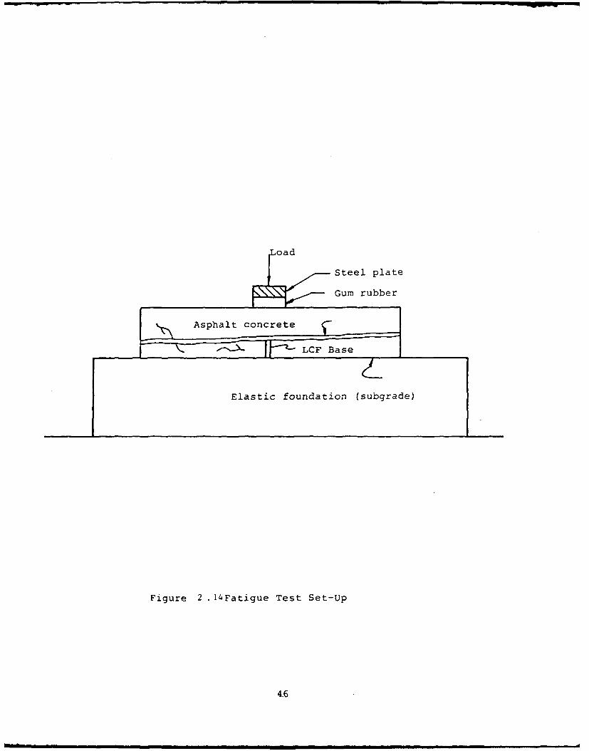
2.8.5 FATIGUE TESTS

Fatigue tests of LCF beams with asphalt concrete overlay are designed to study

the reflection cracking of LCF through the asphalt overlay. The fatigue

experiments were corxucted using a beam on an elastic foundation with geometry

as shcn in Figure 2.14. The selection of this experimental set-up was basedon a two-dimensional modeling of a pavement structure in which beams represent

the pavement and subgrade. The dimensions of the beam and foundation, as well

as the stiffness of foundation, are selected with consideration to simulating

the stress and strain at the bottom of a pavement structure subjected to

traffic loading.

The test set-up is the same as previously used by Resource International Inc.,and researchers at The Ohio State University to study the fatigue properties

of asphaltic mixtures. The fatigue tests were performed using a dynamic loadfunction of Haversine shape. An MIS electro-hydraulic testing system was used

to generate the load factor. To ensure complete recovery of the sample before

the next load cycle, a rest period of 0.4 second was allowed between each load

application.

The duration of load application in all tests was kept constant at 0.1 second.

All tests were performed at rocm temperature (73 OF + 3 OF) and at two stress

levels for each type of specimen.

45

_ _ j

oad

Steel plate

Gum rubber

Asphalt concrete

LCF Base

Elastic foundation (subgrade)

Figure 2. 14Fatigue Test Set-Up

4,6

CHAPIER 3 - IABORATORY TEST RESULTS

3.1 GENERAL RESULTS

The performance investigation of lime + cement + flyash + sand mixtures

included the cimparison of the performance of materials obtained from four

sources and two experimental designs. The first design utilized three

factors; source (Ohio, Oregon, Pennsylvania, and Texas); water pU le "e 15, 7

and 9); and curing time (1,3,7,14 and 28 days at a constant curing

temperature of 140 0 F). There were three independent replicates for each

cobination of factors and the response variables of interest were:

o Unconfined compressive strength, qu,

o Modulus of resilience, Mr,

o Indirect tensile strength, Us,, and

o Fracture toughness, Klc.

The second design also used three factors but was confined to the Ohio source

material only. These factors were niH level (5,7,9), curing time (3,14, and 28

days at constant curing temperature of 140 0F) and treatment (control, Urea and

Glycol). Again, there were three independent replicates for each combination

of factors and the response variables of interest were the same as for the

first design. Also the control data from the first design was used in the

second design for the purpose of cumparison of the properties of the Ohio

source LCF mixture when tested after soaking in Urea and Glycol, the de-icing

materials, for a period of 24 hours prior to laboratory tests. The primary

hypothesis of the second design was to determine whether or not the treatment

with de-icing chemicals had any effect on the response variables while the

secondary hypothesis was to determine whether or not the pH of mixing water

had an effect on the responses.

Discussions in this chapter center around test results of experimental designs

and the identification of any noticeable and consistent behavioral trends of

47

the test data. Summary of all test results in tabular and graphical format

for each source are presented in

Tables 3.1 through 3.5 and Figures 3.1 through 3.16.

However, before discussions concerning the material response cbaracteristics

of the four 10 mixtures are presented, a few remarks concerning the conduct

of the laboratory tests are in order. As stated in section 4.1 all mixtures

were subjected to curing times of 1, 3, 7, 14, and 28 days at a temperature of

140 OF prior to testing. After all tests were ccmpleted, data acquired, and

analyses underway it became apparent that the material characteristic

parameters were responding in an unpredictable manner. This is evidenced by

the fact that almost without exception the values for the response variables

decreased significantly at 28 days cure time and in some instances this

occurred after 14 days cure time. Normally, one would expect the strength of

a concrete mixture to increase with curing time. However, the effect of

maturity, in the form of curing specimens at higher than normal temperatures

over a period of time, is to achieve strength characteristics within a shorter

time period than if the specimens were cured at normal temperatures. It is

also true that subjecting specimens to high temperatures could result in a

loss in strength characteristics after a long period of time if special care

is not taken to provide the proper conditioning envirorment. It is suspected

that each of the specimens tested in this study experienced a loss in each of

its response variables after some period of curing time (probably after 7

days) due to a lack of proper moisture level present during the curing

process.

In an effort to accmiodate this situation the following procedure was

employed. Bers 30 has established the effect of temperature and age, or

maturity, on the strength characteristics of concrete. The maturity, M, is

defined as the product of curing time in hours by the curing temperature in

48

0 0 N r- 0 0 r-N 0co ri ) 0 qv~ L en L. 0

N> r- 0 -4 n a% 0 .4co 0 1-4 %D

4--

41 00 0 0 C 0 0co 0 * A 4 el .

%D 0 .i cv co 0 .4 en 0 0 .

4.0 0

$4 0

.0. 4 co V) 0 0 C%~ U) 0 0 3 LAvi .4 0 kD M L. .4N * I4r, 0 1-4 N N 0 CD NC3 -4

0

(71 %D 0 0 0 N 0 0to1w 0 co LA V) Li .4 0 v co N1 *

Nl co 0 r-4 U) 04 -4 C%

14 cov r 0 0 N 0 0 0 co 0 0

< N- CN -4 N * N r-4 %D N mi

'-44 .- cl co 0 r-4 (n (71 0 1-4 N.0

co UA 0 N L 0 0 N LA) 0 0rl .4 * -4 cl m (n*

-S4 -4

Lo U)

-~- - - - -4 - - r---

C., U -4 *., U -4 z -4>

0.0 0.a Of Or 0 0 .' co 0

el. ~% - -* 4 %x U

49

P. g -4 0D 0 l Go (n 0 % co0N Go M M~ w N

.- 4 -4 4 LA 4 0 -4 0 -

o C)0o co 0 z*- o co -

0h

0 0 0

cs .4 -4 fn 14 4 ~ -4 -

to$4)

0*

U 00 aI)0 LA 0C

* N -4 0 r - .0 CO 0 -4 4 C 0 -4 r-( 10

Ew 0

U) -4 Nol '3 0 %D0

o r0 1

.00

VI) LIC%)L)

0. - C0 N,

- .4 *- . f.

-- L) I) LI -50 U

Ln 0 4 (N K n IV LA q A

*r 00 *0 W 0 co .;. Ch ai

U)0 0 0 o r~LA 0 (N

co -44 N1 ON4 -4 -4 N

to)

0

4.) 04

0 to4 L.. 0 0o 0

0- Nz m 0 *n 0o 41*

%4.)'. -4 N C) -4 LAC4 ~c0 >

t'o

-4 1" -40r=0 0~ 0a. '

LA o9 -1 0 nC; 0 f co ea0*

'4-d.- r4 r4

L -c - e

0>9 >

taoto00.=

LO EU) Q

-4-M

-D CL 0, M 0. ~0. C) C 0 - 0...

S-4 - -4 - - -4 - - W -0- 3a-4 U) -- U) U) u- E. )

~ > -4 0 >1 -4 >9 -

Of~~- mN Ofx :4 O

Ln 0

51

co r- r. i 0 LA co ulA %D N 0ev C4 Ln L LA * l V ON~

,-4 04 Ln- 0~ -4 v

o n ol 0 4 cU r- 0 0 m 0o 0 ' 0 0

.1- sN fN co *'

'4.4 0 N rl r-4 0 Nv fn0 .

to

.4. xw) 0 0 ~--

C)-4 LA 49 -M 00 m~ ON 1 4m r- C) 0 o C 0 N 0 CD N %D LA 0>

'. 14 0D CD4 r 0 -4 C4' .-4 0D -4 -4

0<.41

0000 -w -4 to

-4O 0 N 0 0 N- 0 0 0 "D C 0 0 1enN ~ 0 N * *-4 N * LI)0r- '4 co N ) 0> ' N 0 -4 r-4 1)L

0

$40 -1

0C.

o '30 Li0-t'4 * 0 0 '3D 0 0 0 * 0 0 o(

en ru0I L N 0 %D LA V C A

-4-

E-4 ra

-4-- 4-4-W) U) U) i)-

ti 0 Lo %D 0

0 '0 0. La

0 0z

52

0l c Ln CD N r0o Ch C 0 0 co 0 Ln 0 ~0 0 0

N 0 N 0% C- .-.4o N 0 N

0 0

-W r- LA 0% Lr C)O 0 r- 0 0

CN 0 r .] %0 ~ 0 CN %D 0 N

In

V) 0 K0 0W)r ic %D -4 1,- * 4

o 00 CD o %D 0 0o r- u) 0 DU-) 0C) ~ ~ - .4

C; -4 C;

00

0 4100' 0 0 '0 u 0 C:) 0 W ~ 0 * 0 3

.-4 0D N -4 0 - I - 40.

E 00

>n .4.j

1/a) 41N

LAN -0 4 >- LA 0 ' - 3 0 4

M- a) I 4--4 - 4 wC

0. 0 0V AQ

00-1 el*-

-,4

rep -

-4-- -4 4 53 >4

tto

U)

43

C3)C:%

Co

0)~

og

0 00 0 0

(led) uoleseoio pouisuooun 0

54

0

* E

CO4j

FoU)

0

44

0 0

C.)

0 0 0 0 00 0 0 0>0 LO0 LOc'.J Y-

(led) uoisseadwoC3 pouiuooun0

55

- 2.0

-,

4J0 a-

-u

0)Q

L .. '-

" D0

0 0 0 o O0 0 0 0 co0 to 0 LO cC-4 0

(led) uOlsgeadwoo peuiwuoufl

56

* * 00

* * * __ aE-4

0 C0

0

$-4

* * *LO

0000 0000 0 0 0 0r

LO 0 LO 0O0ocax

(19d) uoisseidwoC) peu!;uooufl

57

C14

0UU)

ar)

LO~

C)

'0 C0 d C5 05

(led) 90+3* sflIfpoiAd goUgiso

58

* C))

* -4

CN >

* Cca

_00

0

0

(Isd) 9O+3* 9flifpopy eouel!998e c0

59

* * 00

* * * -4

* 0

* LO

*0 U )

00

0Oci D c 0 0 0o0CD

(!Sd) 9O+3* sflnpoyyA eauai!qaH

60

0

C*4i

Cq >

* * * *o

* * 0

5 *3 5 5Co

*1d a03 nnoi oals8c

61~

E

co

004~

LO~J 0O"Oc* *C'

* * * * 0

(!d *4MI 91*U. -oJIU Z

* * * ~-~ 0

* * * 0 62

0* * c')

* * C)

* * * *M

* * * co* * *

to O 0 LO

N *~C

* * o

* * * D ..-

(!d *1uol elSgL10 *u

* *L

* * * 63

I0

o _

-

0U

E-4

(-4

00

0 0

(19d) 4;Cuej)S elIsuO.L logjlpul Co

64

E

oCO

-0

LO

HE-

04

L.O

CD

0-2-o

(!Sd) 41UOJI OliSuO.l )lJipuj x

65

co

COO

* IIN

IX4

v$4

0_____ 2 0 0

00

0

(uiI~) ssq~ojGJP66

CJ >

* a

CY)* * ** -o

LO

H-0C)o

CC

67 -

........)

C,* * * * -

* * ** .to

CD

* * *LO

* * 00 0 0 0 0 000 0 0 0 0C

0oc qq- C40

(u!/Isd) sseuLbnflj ainpoeij

68

LO

to

0 0 0 0

0 CD * 114 N* * * ~*-ax

*u/ld ss u4n* *ij i le

69o

degrees above -10 0 C. The value of a strength characteristic, say q, as a

function of M is given by

q=mM+ c (3.1)

where m and c are constants and are determined empirically.

Since laboratory samples were available for curing times of 1, 3, 7, 14, and28 days it was felt that the samples subjected to the lowest curing time (1,3,and 7 days) were, obviously, less affected by the process. Although this is

logical, it is also borne out by the fact that all response variables

decreased significantly after 28 days curing and in some instances after 14

days, as mentioned above. Therefore the test data for all response variablesfor 1, 3, and 7 days were subjected to the maturity function described aboveand each of the response variable values were then predicted at the 14- and28- day periods. This procedure is felt to provide a conservative estimate

for the LCF mixture strength characteristics as a function of cure time.

3.2 UNCONFINED CMPRESSIVE SRENGTH

Test results indicated that unconfined cmpressive strength for all sources

has a fairly uniform rate of strength gain. The Texas source (Table 3.5 and

Figure 3.4) has the largest value of strength, 2250 psi, after the 28 daycuring period followed by the Pennsylvania, Oregon, and Ohio sources. Theselast three sources have approximately the same level of cmpressive strength,

1,400 psi, after 28 days

(see Tables 3.2, 3.3, and 3.4 and Figures 3.1, 3.2, and 3.3).

3.3 MDUIJUS OF RESILIENCE

Test results for modulus of resilience are presented in Figures 3.5 through3.9 and Tables 3.2 through 3.5. These results indicate that the Pennsylvania

source has the largest value for Mr, slightly greater than 1.4 x 106 psi, at

the 28- day period. The Texas and Ohio sources have about equal values of Mr ,1.0x10 6 psi, followed by the Oregon source whose Mr value is about 0.8x10 6 psi

70

after 28 days curing time.

3.4 INDIRECT TENSILE STREWTH

Test results for Indirect Tensile Strength are graphically presented in

Figures 3.9 through 3.12 and listed in Tables 3.2 through 3.5. These data

indicate that the Texas source achieves the highest level for t , about 290

psi, after the 28- day cure period. The Oregon source achieves about 250 psi,

followed by the Pennsylvania source at 220 psi and lastly the Ohio source at

180 psi for y after the 28 day period.

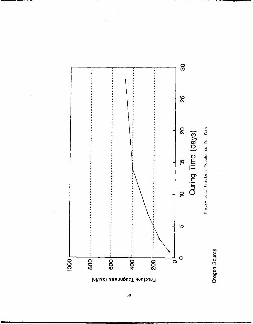
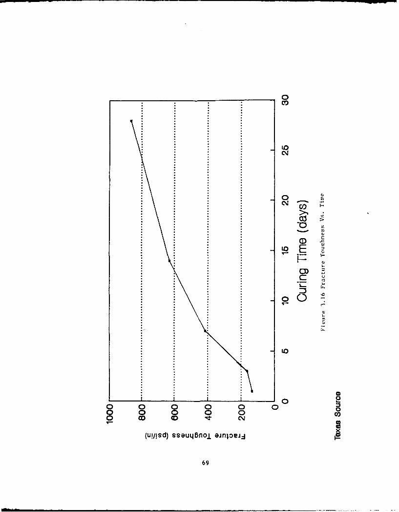
3.5 FRACTURE TCUGHNESS

Test results for fracture toughness are graphically presented in Figures 3.13

through 3.16. These data reveal that the Texas 1CF source specimens achieve

the highest value for Klc, about 875 psi in 1 / 2 (Figure 3.16), followed by the

Oregon and Ohio sources at the 450 psi inl/2 level (Figures 3.13 and 3.15),

and last the Pennsylvania source at the 300 psi inl/ 2 level (Figure 3.14)

after the 28 day cure period.

3.6 EFFECT OF DE-ICING CHEMICALS

As explained in section 2.8 two treatments (Urea and Glycol) were employed to

determine what effect de-icing chemicals have on the material response

characteristics of the LCF mixtures. A sumarxy of the original laboratory

test results for the treated samples is presented in Table 3.1

Ccuparison of response parameters qu, Mr and O for samples treated with de-

icing chemicals with the results for untreated samples indicates that there is

a loss of strength in the treated samples. However, the de-icing chemicals

appear to have no impact on the measured value of the fracture toughness, Klc.

There is also no significant difference between Urea and Glycol treatments for

each of the response parameters measured. That is, the Ohio source LCF

mixture response parameters, qu, Mr, 0y and Klc, have (practically) the same

71

values whether treated with Urea or Glycol.

3.7 EFFECT OF WATER PH LEVEL

The water pH level was varied to determine what effect this factor has on the

material response characteristics of the Ohio LCF mixture. The results of

these tests, including predicted values where appropriate, are presented in

Tables 3.1 through 3.5.

These results were also subjected to the same analyses procedure mentioned in

subsection 3.6 for the sane purpose, i.e., is there a statistically

significant difference in the response characteristic of the Ohio LCF mixture

due to water pH level.

The outco of this analysis indicated that the water pH level did not have a

significant effect on the material response characteristics over the range of

pH levels and sample ages tested.

Since the results of the foregoing analyses indicated that LCF mixture

material response characteristics do not depend on water pH level, the

graphical presentations of the laboratory results, Figures 3.1 through 3.16,

for the four LCF sources are presented as average values for the variable over

the three water pH levels.

3.8 FATIGUE

3.8.1 FATIGU1E TEST RSULTS

Before the start of the fatigue tests, it was expected that the test results

would resemble a standard fatigue pattern. That is, the expected pattern was

expected to follow a standard S-N curve, approaching the fatigue limit

asymptotically.

However, it became apparent during the tests that the LCF beam specimens were

not responding in a manner typical of accepted beam fatigue behavior. The

72 1

results are shown in Table 3.6. They appear to indicate that there was almost

no low- cycle fatigue behavior for the LCF beams.

The only reliable information obtained for the low- cycle behavior was the

static strength of the specimens.

At load levels lower than the load corresponding to the value for flexural

strength, the fatigue life of the specimen appears to be independent of the

load level. The slope is zero for the line representing the relation between

applied dynamic load the number of cycles to failure. The transition from low

to high cycle fatigue is so abrupt that it has not been discernable in testing

of the specimens. The abrupt failure is assumed to be a result a very short

time between the initiation of cracks of the specimen under load, and the

spread of the cracks to a great enough extent to cause failure.

3.8.2 SUGGESIONS FOR ADDITIONAL FATIGUE TESTS

Other more elaborate techniques to monitor crack initiation and growth are

available but were beyond the scope and cost of this study. Stress coating,

trip gages, and acoustic signature techniques have been used for this purpose

in the past and in current fracture related research

73

Table 3.6. Fatigue and Flexural

Test Results for LCF Specimens

LOAD, 1B NOR4. LOAD, PSIWF SPECME NI

SOURCE THICKNESS FLEXURE FATIGUJE THICKNESS FLEXURE FATIGUEINCHES INCHES(A/C+LCF)

Ohio 1 + 2 213 2.7 29

Ohio 1.5 + 2 251 3.1 27

Penn 1 + 4 505 4.7 23

Penn 1 + 3 233 3.7 17

Penn 1 + 4 370 4.7 17

74

studies and could be employed in a more complete investigation of fatigue

fracture of ICF pavement materials.

In addition, there is evidence that pavements that support moving traffic,such as runways, are subjected to stress reversal. That is, as the aircraft

load noves past a point on the pavement, that point is alternately subjected

to tension and compression. A fatigue test could be designed that wouldsubject the samples to stress reversal and would be more representative of the

stresses to which the pavement might be subjected when exposed to moving

traffic.

75

CHAPrER 4 - DESIGN AND CONWUCT OF FIELD TESTS

4.1 OBJECIVE

The objective of the field test activities was to study the long-term changes

in the behavior of LCF pavements that may occur as a result of pozzolanic

activity and envirormental forces. In order to accumplish this objective core

samples were obtained fram four airports. They were analyzed for the effects

of pavement age on modulus of resilience and unconfined ccnpressive strength.

4.2 PREVIOUS RESEARCI

The curing of LFA is controlled by three factors: time, moisture, and

temperature. Each directly iracts the pozzolanic reaction and must be

controlled to ensure proper setting and ccmpressive strength.

MacMurdo and Barenberg 12 conducted extensive tests on the effects of time and

temperature on LFA pavements. The results are shown in

Figure 4.1. As can be seen fram the figure, the effect of temperature on the

cupressive strength is not linear.

It is important to consider the effects of temperature on curing when planning

LFA placement. Adequate curing mist be obtained prior to the beginning of

cyclic freeze-thaw to assure satisfactory field perfomaznoe. 13 Curing

conditions should be specified with the purpose of producing at least the

minimun LA mixture strength.

IA mixtures cared for 7 days at 100°C (under ASTM C593 conditions) have

exhibited strengths ranging frcm 500 psi to 1000 psi. After 1 to 2 years

these values may exceed 1500 psi and ultimately maybe in excess of 3000 psi. 7

Though ultimate strengths are fairly high, many engineers feel that the slow

rate of strength development is undesirable and is a function of the slow

dhemical reaction between lime and flyash. To ccmpensate for low early

76

1800

1600 1d

10C

-~ 1200

C

C,

E(0

0 600

200

0

0 10 20 30 40 50 60 70 80 90 100 110

Curing Time, days

Figure 4.1 Effects of Curing Time and Temperature on the StrengthDevelopment of a Lime- Flya sh- Agg regat e Mixture (12)

77

strengths, admixtures are used to accelerate early strength gains. Portland

cement has proven effective in this requirement.

Under proper curing conditions, chemical reactions in LFA mixtures will

continue as long as sufficient lime and flyash are present. 14

Figure 4.2 shows compressive strength growth with age of a LFA mixture in the

Chicago area.

4.3 A2PROA

TO acouplish the field test activities two tasks were undertaken; core

extraction and core testing. A summary of these tasks is presented in the

following paragrap±hs.

4.3.1 EXTRACTION OF CORES

Test cores waze taken frum LFA pavements at Portland Airport, and LCF

pavements at New York and New Jersey Airports. At each airport, test cores

were taken frum two taxiway areas with three points per area on the selected

pavements, 500 feet frum one end and in the middle. At each point the test

cores were extracted from the keel section and the left and right pavement

edges.

In 1986 project representatives visited the offices of the Port Authority of

New York and New Jersey and met with the airport planning, design, and

maintenance engineering staffs. At that time, the goals and objectives of the

LCF study effort were presented and suport was requested in extracting sample

pavement cores at JFK and Newark Airports. Each of the Port Authority

organizations agreed to support the study. All extractions and refilling of

pavements were to be done by Port Authority engineers.

Later in 1986 project personnel visited Portland International Airport to

arrange and coordinate the extraction of LCF cores fru the site runway. It

was agreed at the meeting that seven (7) full depth cores would be extracted

from Ianyway 10R.

78

2000 Strength

development

2nd and 3rdyears

1600 1 /

CStrength

developmentC1st summer

1200.

Y Dormant

0 A 1st winterf A

E 800 •0

Initial/ / strength

400 developmentSept. construction

0/

110 100 1000 10000

Age in days

Figure 4.2

Compressive Strength Development of Lime-FIlash-StabilizedMixture in Chicago Area (16)

Courtesy: Alberg and Barenberg, "Pozzolanic Pavements," Bulletin 473,Eng. Experiment Station, University of Illinois (1965)

79

The coring process at Portland Airport was completed in 3 hours. The coring

was done by Concrete Coring of Vancouver, Washington. Seven cores were

extracted frum the locations given in Table 4.1. Core locations were chosen

in order to assure collection of samples from areas with heavy, moderate, and

light volumes of traffic.

None of the cores was damaged by the extraction process. The only breaks

occurring in the full depth cores were the natural separations occurring

between lifts.

Cores 1-6 were marked, wrapped, sealed, boxed, and shipped to Tuskegee

University to be tested. Core 7 was sent to Northwest Testing Laboratories,

Inc. of Portland, Oregon, to be tested as a reference sample. This reference

helped validate the testing done at Tuskegee University and also provided

verification that no damage occurred to the cores during their transport.

In April of that year project personnel visited the New York World Trade

Center to meet with representatives from the Port Authority of New York and

New Jersey to finalize the plans for core removal at Newark and JFK Airports.

At the meeting, it was agreed that cores would be extracted at JFK Airport

later that month. Similarly, core extractions would begin at Newark Airport

the next day after campletion of the JFK extractions.

Eleven cores were extracted at JFK and labeled No.'s 8 through 18. Cores #8-

#14 and #18 were boxed and shipped to Tuskegee University. Cores #15, #16,and #17 were sent to the Port Authority's materials lab for testing. Figures

4.3 and 4.4 show the location of each core extraction with respect to the

taxiway frrm which they were extracted. Shown in Figure 4.5 is an overall

layout of the airport.

JFK Airport had experienced slippage of the wearing course over the IcF base

course on some of the taxiways. These areas were described by the

representatives as looking like waves in the pavement. At this point it was

determined that coring at these locations may give some insight into why this

80

Table 4.1

Portland Extraction Matrix

Core Number Location Lift Designations

1 500 ft. from end of runway; A, B70 ft. left of centerline

2 500 ft. from end of runway; A, B, C10 ft. left of centerline

3 500 ft. from end of runway; A, B, C10 ft. right of centerline

4 1,200 ft. from end of runway; A, B70 ft. left of centerline

5 1,200 ft. from end of runway; A, B, C10 ft. left of centerline

6 1,200 ft. from end of runway; A, B, C10 ft. right of centerline

7 1,400 ft. from end of runway; A, B, C10 ft. left of centerline

81

Fijxure 4. 3

JFK Core Locations, April 21, 1986

Taxicrossing "LA"(

LA

"Cross Section"

Outer #8

Taxiway #0 #9

r'1 0'

'#10

#9

'#8 #8 A & BLlyers

#9 B & C Layers

#10 - Discarded10' #11 - A, 8, C Layers

#11

82

Figure 4.4

JFK Core Locations, April 22, 1986

Plan

rTaxicrossing "N"

N

5'XCross Section"

#12"1

Outer *#13

Taxiway # #14

,#1310, #14

#16.

018o

-.12 - A Layer

10' n1 - A & B Layer

"14 - A Layer

#15 - A & B Layer

#16 - B Layer

Taxicrosssing "MAV

00 11 32 17181

841

Ti.-

R.

P4 -- 9

N

M .

L IS

JA~D AA I'-

cotRTA I Is~I A _ ~- -

858 FAA

15 16 17H18.1912 2 21J22 2324125 26 27

Sal

V84

T AV- U0 t AIORT DATA

IAOT ELEVATION .12 FT ADM9

T EAR SEA LEVEL AT AWN HOOK. N.J.* AptPORT REFERENCE POINT (AMP) -

A S CORWTSLAY 40'38'28J"COIAE"LONG. 73-46' 41A"'

- - 4

R _

APPIMATE LOCAION at

TELCO FIEW TELEPHNE tEA

I 0-, -> w 'I$

Ils

-- 2 M

jot ~ l LLA -t~gL S

854

BA ***"~as

A HGV5

+. ... -.

ft _ >

Avato C00n Divsio

" FAA

lI~t ~ -- Zii~~ AN

51 16 17 1 1 2 3 405 2,21. -

85/86 Figure 4.5

problem occurred and if it was ICF related. Cores were taken from the tops

and valleys of the waves, and at areas where no waving occurred (this is shown

in the "cross section" in Figure 4.3).

Extraction of three ccmpleted layers (A, B, and C) from each site was rare.

Most cores experienced at least one layer that was cracked; fractured or

damaged. These conditions were experienced in all the areas where cores were

extracted, not just in the areas where waving had occurred. It should be

noted that the cracking and fracturing that occurred in the cores pointed to

the possibility of fatigue of the LCF base course.

In some cases the bottom layer ("C") was not found. One possible explanation

for this is the length (approximately 14") of the coring bit used. Initially

the core extraction method used involved extending the core bit through the

entire depth of the pavement (to cut the core layers) and then trying to

retrieve each layer. This method may have forced the "C" layer into the

subgrade, causing it not to be retrievable. This procedure was changed at

Newark Airport, where coring was only to the depth of the bottom of the "C"

layer. Results for acquiring all three layers improved. It should be

mentioned that the core extraction at Portland Airport used a 36-inch bit and

no problem were encountered recovering any layers.

Nine cores were extracted at Newark International Airport from the locations

shown in Figures 4.6, 4.7, and 4.8. Figure 4.9 is an overall layout of the

aLport. The cores were labeled Nos. 19 through 28. Cores #19 through #23 and

cores #25, #27 and #28 were sent to Tuskegee University to be tested. Cores

#24 and #26 were given to the Port Authority for testing. The results fran

these tests were used to validate testing at Tuskegee.

a37

Figure 4.6

Newark Core Locations, April 23, 1986

U

#19 - A, B Layers

#20 - A, B Layers

Taxiway #21 - AYankeeora Y Y #22 - A

Y(built 1976)

0'i #22

10,

-TTso, : ;

S

88

Figure 4.7

Newark Core Locations, April 24, 1986

U

_ #231"-- 10'

is, #23 - A, B, C Layers

#2 4 I#24 - A, B, C Layers

Taxiway Y YYankeeor

Y

S

89

Figure 4.8

Newark Core Locations, April 24, 1980

#25 - A, B, C

#26 - A, B These cores were extracted from theapron of Terminal "C"

#27 - A, B

0 Taxiway Between Taxiway Crossings E & RD (built 1970)

E RD

#28 - A, B, C Layers

#28

0 Taxiway

90

ITM

-w -Sp -

SAW ,;1

"MOTE OT654 I PAS ENGER TE MINAL A I m 25 N T IO A E T L M A M N L O. 1 550A M AH01 ,1 G U R O T HI C 0 .

514 7LOTDOLLROTHMOs~w,

GB LlA OI.PLC I7 ETsIYITTO 1 4 GADPS Ii .. 101

SLGEI 2 P . T~T L 7 P . A N S O A E0 7 G A D P S 4 14 1 1

J 4 I P . M INL GAR GE 2 4 RI CIR CAL 4~ 4 R P. .IA N AI~~t 104 06 LOG 01 94 UAR PO T 6i9 11 lJI

osI S I R TI AIM H N A 7 4 WTH H UIN . 2 P VE G LG 3 9 U R o r,419 11 1C * U S ~ b. H A N A R 13 6 C NT AL IAT N G RI RIO LA N J 4 6 P A M A N?. GAR GE 2 2 A. AIH 5 ~ 4 ~ 6 19 ON1 4 21 ~ l~t VI TIO J 1 4 PA H AVI G A14 , S 4 P . L NOI AP NG TO ACE AL O. S iRE TOL B OTH LO 1 ~POSTUM0D 25~c 00rl

ETLCRAMN LG H2S A AN.H4U NRHPSSNE EMNLH23 IETINVLIA S IC U 24 SU IZ ER IM CA M IN . ~ f . s 52 Wf RR IA SO C & 9 UA D OS ( NA TI E)G i 5 IN hA ~ g j 0 1 1WAI-4 9. UAD OS DI IE TGARPRS~uAN h lLL W~ E~ 121I

PS 15 AIR

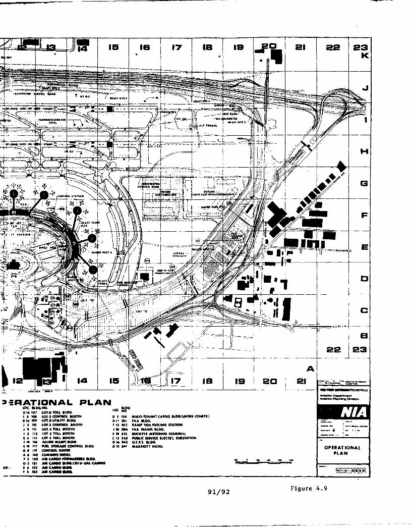
~1L 14 7 i9 j1~ 2 222

-SISSUKI ~~~ .V~ NO- . SI ilS U_____ ______ As

f~tva AL SU S A

LSSFa2 H41 9 02 i.-

~RATIO AL PLASIDO

5100. OC NOA 2 obw92CFUL101 5 U.ITNN CRO1004( O4L094 09 11.0 TIL~Y IO. 01 20 "AMai02 ~ ~ ~ ~ o $ID @0.AMRLSOT

I23 APYN uLN AI#

11 0.011 COT lFOl

F I IS) A MCIIO

91/9 Figre4.

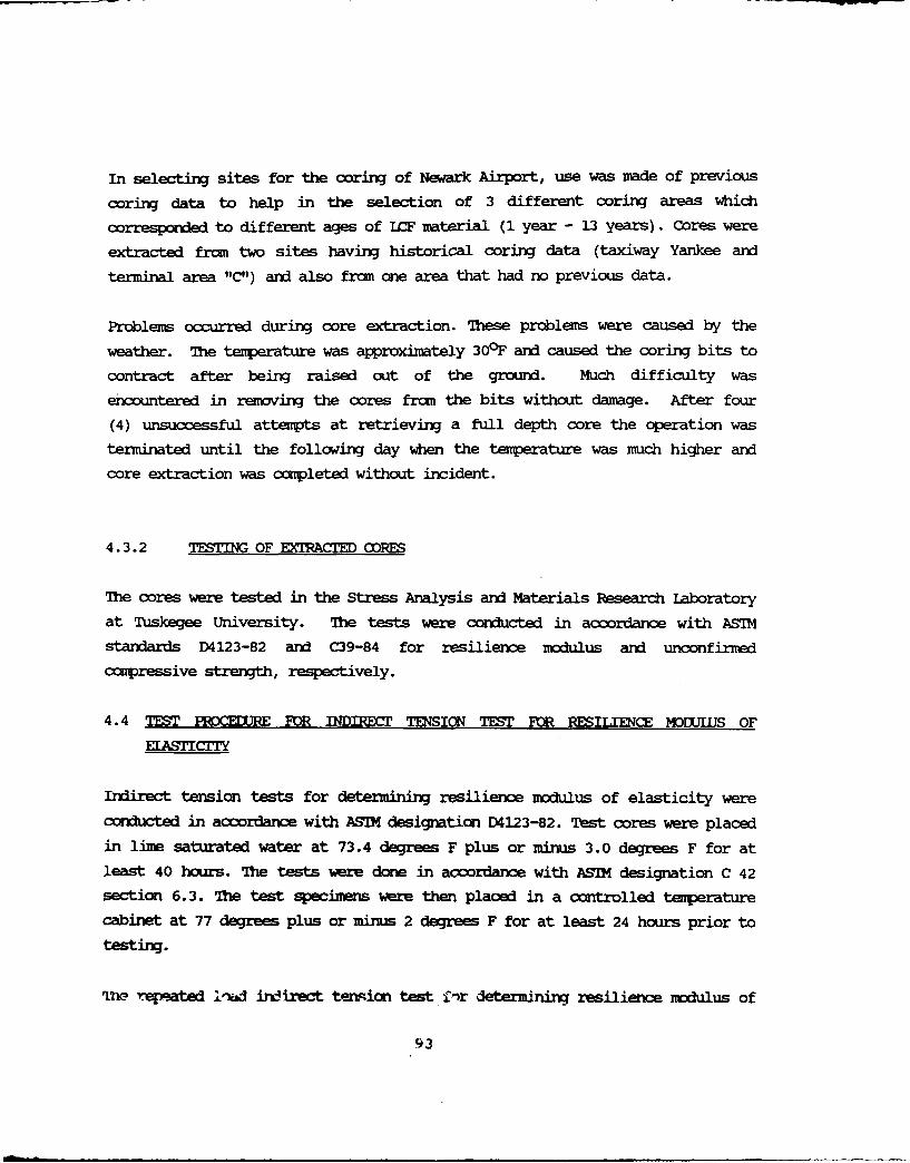
In selecting sites for the coriM of Newark Airport, use was made of previous

coring data to help in the selection of 3 different coring areas which

corresponded to different ages of LCF material (1 year - 13 years). Cores were

extracted from two sites having historical coring data (taxiway Yankee and

terminal area "C") and also frao one area that had no previous data.

Problems occurred during core extraction. These problems were caused by the

weather. The temperature was approximately 30°F and caused the coring bits to

contract after being raised out of the ground. Much difficulty was

encountered in removing the cores fru the bits without damage. After four

(4) unsuccessful attempts at retrieving a full depth core the operation was

terminated until the following day when the temperature was much higher and

core extraction was campleted without incident.

4.3.2 TESTING OF EXTRACTED CORES

The cores were tested in the Stress Analysis and Materials Research Laboratory

at Tuskegee University. The tests were conducted in accordance with ASTM

standards D4123-82 and C39-84 for resilience modulus and unconfirmed

cupressive strength, respectively.

4.4 TEST IRCEXM FOR INDIREC TENSION TEST FOR RESILID=CE MDXJUJS OF

ELAWTICIri

Indirect tension tests for determining resilience modulus of elasticity were

conducted in accordance with ASIM designation D4123-82. Test cores were placed

in lime saturated water at 73.4 degrees F plus or minus 3.0 degrees F for at

least 40 hours. The tests ware done in acordance with ASIM designation C 42

section 6.3. The test specimens were then placed in a controlled temperature

cabinet at 77 degrees plus or minus 2 degrees F for at least 24 hours prior to

testing.

'111o repeated inad in-irect tension test f-r determining resilience modulus of

93

concrete cores was conducted by applying campressive loads in a haversine wave

form. The load was applied vertically in the vertical diametral plane of a

cylindrical specimen of concrete. The resulting Poisson's ratio and resilience

moduli were calculated using values for measured deformation.

4.5 APP-ARNUS

4.5.1 TESING MACINE

The test machine used was MIS Model 810 which has a function generator Model

410 capable of producing the desired wave form.

4.5.2 DEFOITION MEASURMNS

The values of the vertical and the horizontal deformations were measured using

the X-Y recorder and Linear Variable Differential Transducer (LVDT). The LVDT

was fixed at the mid height of the specimen.

4.5.3 WADING STRIP

A pair of metal loading strips with a concave surface having a radius of

curvature equal to the nominal radius of the test specimens was made to apply

load to the specimen. The dimensions of the loading strip were designed in

accordance with ASZM designation D4123.

4.5.4 CAPPING

The capping plates which were used to cap the core ends were made in

accordance with ASIM designation C617.

Ccumpression Platen MIS Model 643.41B grip was used to test concrete cores.

94

4.6 TEST pRcEIRE FOR RESILIENCE MDDUIJS TEST

The test specimens were placed in a controlled temperature cabinet and heated

to the test temperature. The specimens were kept in controlled temperature at

least for 24 hours prior to testing. The diameter and length of the cores

were measured before testing.

The specimens were placed in the loading apparatus. They were positioned so

that the loading strips were parallel and centered on the vertical diametral

plane.

The specimens were preconditioned by applying a repeated haversine waveform

load to the specimen without impact for a minimum period sufficient to obtain

uniform deformation readout. The minimum load was determined so that the

resilient deformation was stable. Each test specimen was tested at three

loading frequencies: 0.5HZ, 1.OHZ, and 2.5HZ.

The horizontal and vertical deformations were monitored during the test. If

the total cumulative vertical deformation was found greater than 0.001 inch

during the test then the applied loads were reduced.

The resilience modulus tests were completed within 4 minutes from the time the

specimens were removed frin the temperature-controlled cabinet.

4.7 TEST PRCEERE FOR UNCNF iED CCZHPRESSION TEST

The diameter and length of the specimens were measured after taking them out

fram the saturated lime solution.

The end surface of the specimen was capped with a sulpihur mortar capping

compound in accordance with AST1 designation.

The specimens were placed in the lower platen of the grip MiS model 643.41B.

The rate of loading was set such that the moving head travelled at a rate

approximately 0.05 i-/irdn. Load was ai'vlied continuously and withcxt shock.

95

The load was applied until the specimens failed. The maximum load carried by

the specimen during the test was recorded with the help of an X-Y recorder.

96

CAPTER 5 - FIELD TEST REUS

5.1 GENERAL RESUITS

Because of the results of previous research, it was expected that the fieldtest results would confirm that LCF pavements exhibit increasing strength asthey age. This was only partially confirmed.

Figures 5.1 and 5.2 and Tables 5.1 through 5.4 represent the results of testsof modulus of resilience and unconfined compressive strength for core samplestaken from the runway pavements that were tested.

The samples taken from Newark Airport had ages of 3, 10, and 16 years at thetime of testing. The compressive strength test results for Newark showed thegreatest strength for the ten year old samples. The resilience modulus forthe Newark samples was greatest at 16 years.

For both copressive strength and resilience modulus, the samples fromPortland Airport showed the highest test results. The test results for JFK

were low for compressive strength and resilience modulus.

These results may have been influenced by exposure to differing environmental

conditions (e.g. temperature, chemicals), mix design or other factors.Analysis of these factors was beyond the scope of the project. However, itwould appear that further information could be gained by testing samples from

the same pavements several times as they age.

9"i

Na, ma

PueT42o

PUleAeN E.

0.. L§

(I-d) yA15u@J -A-7-aidLuc -

98

........................

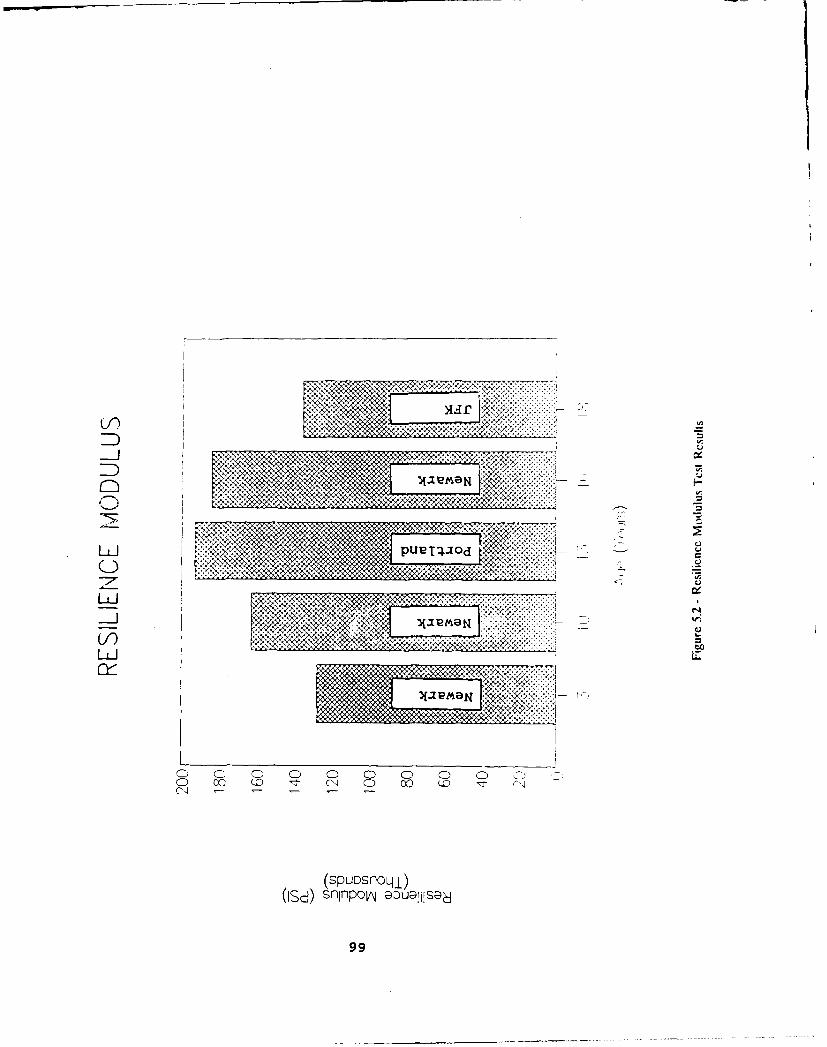
ot

LL-C

C) ( 0 0 C 0 0 00 (i ( ~- C'- C0 0D (. Q (

(d)(spuosnoujj)sflifpoV @DuailisG~

99

Table 5.1

COMPRESSION TEST RESULTS

SAMPLE SOURCE LAB AGE DIAMETER LENGTH STRENGTHyrs in in psi

1A Portland Tuskegee 13 2.6 5.3 2754

1B Portland Tuskegee 13 2.6 5.2 1705

2A portland Tuskegee 13 2.6 5.2 2594

2B Portland Tuskegee 13 2.6 5.3 3337

2C Portland Tuskegee 13 2.6 4.1 3182

3A Portland Tuskegee 13 2.6 5.3 1324

3B Portland Tuskegee 13 2.6 5.3 3024

3C Portland Tuskegee 13 2.6 5.3 2502

4A Portland Tuskegee 13 2.6 5.3 2429

4B Portland Tuskegee 13 2.6 5.3 1360

5A Portland Tuskegee 13 2.6 5.3 1117

5B Portland Tuskegee 13 2.6 4.3 2026

5B Portland Tuskegee 13 2.6 4.3 1429

5C Portland Tuskegee 13 2.6 5.5 3050

6A Portland Tuskegee 13 2.6 5.2 1930

6B Portland Tuskegee 13 2.6 5.3 1800

6C Portland Tuskegee 13 2.6 5.4 2412

8A JFK Tuskegee 18 2.6 5.4 2682

8B JFK Tuskegee 18 2.6 5.3 703

9B JFK Tuskegee 18 2.6 5.3 1290

9C JFK Tuskegee 18 2.6 3.6 536

11A JFK Tuskegee 18 2.6 5.2 750

1IB JFK Tuskegee 18 2.6 3.1 585

IIC JFK Tuskegee 18 2.6 5.2 864

12A JFK Tuskegee 18 2.6 4.9 1381

13A JFK Tuskegee 18 2.6 5.3 1410

13B JFK Tuskegee 18 2.6 5.4 1498

14A JFK Tuskegee 18 2.6 5.3 1510

18A JFK Tuskegee 18 2.6 5.4 1516

19A Newark Tuskegee 10 2.6 5.4 2051

20A Newark Tuskegee 10 2.6 5.4 2317

20B Newark Tuskegee 10 2.6 5.1 1340

21A Newark Tuskegee 10 2.6 5.4 2515

22A Newark Tuskegee 10 2.6 3.4 2330

22A Newark Tuskegee 10 2345

23A Newark Tuskegee 10 2.6 5.4 2025

23B Newark Tuskegee 10 2.6 5.3 1340

23C Newark Tuskegee 10 2.6 4.3 1731

25A Newark Tuskegee 3 2.6 5.3 2943

25B Newark Tuskegee 3 2.6 5.2 1704

25C Newark Tuskegee 3 2.6 5.4 1201

27A Newark Tuskegee 3 2.6 5.4 1390

27B Newark Tuskegee 3 2.6 5.2 1880

28A Newark Tuskegee 16 2.6 5.4 2151

28B Newark Tuskegee 16 2.6 5.2 1518

28C Newark Tuskegee 16 2.6 3.4 1976

100

Table 5.2

COMPRESSION TEST (FIELD)RESULTS VS. AGE OF PAVEMENT

STRENGTH

AGE AVG MIN

(yrs) (psi) (psi)

3 1823.6 1201

10 1999.3 .1340

13 2233.8 1117

16 1881.7 151818 1227.1 536

101

Table 5.3

RESILIENCE MODULUS TEST RESULTS

RESILIENT

SOURCE LAB AGE DIAMETER LENGTH MODULUSyrs in in psi

Portland Tuskegee 13 2.6 5.3 112,391Portland Tuskegee 13 2.6 5.2 74,712Portland Tuskegee 13 2.6 5.2 118,746Portland Tuskegee 13 2.6 5.3 155,464Portland Tuskegee 13 2.6 4.1 155,178Portland Tuskegee 13 2.6 5.3 130,454Portland Tuskegee 13 2.6 5.3 83,698Portland Tuskegee 13 2.6 5.3 225,153Portland Tuskegee 13 2.6 5.3 575,755Portland Tuskegee 13 2.6 5.3 140,692Portland Tuskegee 13 2.6 5.3 114,134Portland Tuskegee 13 2.6 4.3 509,279Portland Tuskegee 13 2.6 5.5 97,542Portland Tuskegee 13 2.6 5.2 410,779Portland Tuskegee 13 2.6 5.3 75,721Portland Tuskegee 13 2.6 5.4 106,370JFK Tuskegee 18 2.6 5.4 169,870JFK Tuskegee 18 2.6 5.3 274,330JFK Tuskegee 18 2.6 5.3 98,486JFK Tuskegee 18 2.6 3.6 177,709JFK Tuskegee 18 2.6 5.2 181,144JFK Tuskegee 18 2.6 3.1 149,100JFK Tuskegee 18 2.6 5.2 79,887JFK Tuskegee 18 2.6 4.9 110,926JFK Tuskegee 18 2.6 5.3 125,664JFK Tuskegee 18 2.6 5.4 88,212JFK Tuskegee 18 2.6 5.3 84,675JFK Tuskegee 18 2.6 5.4 83,688Newark Tuskegee 10 2.6 5.4 98,303Newark Tuskegee 10 2.6 5.4 156,047Newark Tuskegee 10 2.6 5.1 234,380Newark Tuskegee 10 2.6 5.4 138,261Newark Tuskegee 10 2.6 3.4 278,042Newark Tuskegee 10 2.6 5.4 119,813Newark Tuskegee 10 2.6 5.3 78,463Newark Tuskegee 10 2.6 4.3 199,045Newark Tuskegee 3 2.6 5.3 104,159Newark Tuskegee 3 2.6 5.2 135,840Newark Tuskegee 3 2.6 5.4 105,141Newark Tuskegee 3 2.6 5.4 161,160Newark Tuskegee 3 2.6 5.2 131,045Newark Tuskegee 16 2.6 5.4 158,386Newark Tuskegee 16 2.6 5.2 135,582Newark Tuskegee 16 2.6 3.4 258,105

102

Table 5.4

RESILIENCE MODULUSVS. AGE OF PAVEMENT

COMPRESSIVESTRENGTH

AGE AVG MINyrs psi psi

3 127,469 104,15910 162,794 78,46313 192,879 74,71216 184,024 135,58218 135,308 79,887

103

5.2 FIELD TET E9T CXLURS

Resilience modulus of elasticity was calculated by using horizontal and

vertical deformation at frequencies of 0.5, 1.0, 2.5 Hz. The value of

resilience modulus was calculated and the average of these was taken. The

calculated resilience 3 modulus was calculated and the average of these was

taken.

The compressive strength of the specimen was calculated by dividing the

maximum load carried by the specimen during the test by the average cross-

sectional area of the specimen. Sample calculations are shown in the

following sections.

104

5.3 Samle Calculation for Resilience Modulus for Core 2A

The total modulus of resilience ERr was calculated as follows:

ERt = P ( g + 0.27 )/t dHt

where

g = 3.59 d - 0.27

g = Total resilient poisson's ratio

dHt = Total recoverable horizontal deformation

dvt = Total recoverable vertical deformation

P = Repeated load

t Thickness of specimen

Result:

Frequency (Hz) .5 1.0 2.5dHt (in) 0.000125 0.000115 0.0000675

dvt (in) 0.00056 0.00052 0.00045P (lbs) 87 87 87t (in) 2.65 2.65 2.65g 0.5314 0.524 0.2685ERt (psi) 210,465 226,654 261,911

Average Resilience Modulus = 210,465 + 226,654 + 261,911 = 233,010 psi

5.4 Sample Calculation for Unconfined C9zmIression Test for Core 2C

D = 2.63 in = Diameter of core

L/D= 1.57 = Ratio of length to diametercf = 0.96 Correction factor for I/D

P = 18,000 = Iad at sample failure

A = 5.43 in. = Area

P/A = 3315 = oMpressive Strength

Corrected CQmpressive Strength = 3315 x cf = 3315 x 0.96 = 3182.0 psi

105

- mm mm ~ mi

CEAPE 6 - sL= = E WF PAVEM r DSIG NJIDEMlT S

6.0 APPROACH

The design approach for WCF pavements must consider the fact that LCF

pavements exhibit the characteristics of a flexible pavement just after

construction and become rigid pavements as they mature. Engineers of the Port

Authority of New York and New Jersey developed a design method which

incorporated the dual characteristics of WCF pavements. The analysis

presented in this report for the design of WCF pavements is similar to that ofthe Port Authority2 6 with the following exceptions.

o LCF strength characteristics that resulted from the tests are

available for preliminary design and planning.

o Equations for calculation of the maximum tensile and ccmpressive

stresses imposed by an aircraft load on a pavement slab are expanded

to take into account the location of the load relative to the edges

of the pavement.

lob

The basic concept involves looking separately at specific design

characteristics of rigid and flexible pavements. The final design is derived

by taking the greater thickness determined by the separate analyses.

The objectives of the approach are several: minimize the likelihood of

pavement failure over a long service life (20 years), minimize aircraft and

pavement vibration, minimize the need for pavement maintenance that may

disrupt traffic flow, and maximize economy in the use of material, equipment,

and manper resources.

In order to attain these objectives, the approach attmpts to accomplish the

following:

Aircraft and pavement vibration are minimized in order to promote passenger

comfort and to extend the life of the pavement. The design approach minimizes

ccmpaction and horizontal displacement of the subgrade and maintains

substantial separation between the natural wavelength of vibration of the

aircraft and the wavelengths of any significant pavement surface deviations.

The need for pavement maintenance is minimized by keeping low the likelihood

of pavement rupture caused by either fatigue or inability to withstand

instantaneous loads. The design approach considers the effects of pavement

flexure during many aircraft operations and the ability of the pavement to

withstand compression and tensile loads.

Economy is achieved through minimizing the quantity of paving materials while

designing to meet performance objectives, and minimizing manpower and

equipment costs required for maintenance and repair.

The steps of the recommeded design approach are as follows:

1. Determine the pavement thickness based on control of aircraft and

pavement vibration response

2. Determine the pavement thickness based on elastic mass analysis

3. Determine pavement thickness based on stress, strain, and strength

relationsJ ps:

107

- Tension

- c~Opression

4. Determimn the pavement thickness based on fracture toughness

5. Select the maximum thickness determined in steps 1 through 4, above

6. Add a margin of safety

6.1 PAVENT DESIGN BASED ON ONTROL OF AIRCRAFT AND PAVME VIERATION

RESPONSE

Port of New York Authority design methods are recanerxed to be adopted for

control of aircraft and pavement vibration response. These methods assume the

following conditions for vibration response to be held within a range of

acceptable passenger comfort.

Vibration response of an aircraft in motion along a pavement is a function of

the pavement roughness, aircraft velocity, and the natural frequency of the

aircraft. It is conveniently modeled as the acceleration of the aircraft in a

direction normal to the pavement.

The simplest model of aircraft/pavement interaction occurs with the aircraft

moving across a smooth pavement. Aircraft vibrations caused by its motion and

the rotation of its machinery become driving function for the vibration of the

pavement. The pavement vibrates in response to excitation by the aircraft.

In normal use, the pavement is not smooth but develops surface deviations over

time due to the stresses of use. The second model of vibration response has

pavement roughness as a forcing function and aircraft vibration as a response.

In the third level, the aircraft and pavement are responding to each other.

The allowable surface deviation (*) frcm a smooth plane as a pavement

approaches the limit of its planned service life is related to the velocity

and natural frequency of the aircraft and to the length of the deviation by

* Y / 2 (6.1)

108

in whichf

K = .63 DI ( 6.2 )v

and]

DI = tolerance for mean vehicle response

f = natural frequency of the aircraft

v = aircraft velocity

L = wavelength of the surface deviation

In this expression L is assumed to be that significant wavelength that, at the

aircraft velocity, causes aircraft vibrations at the natural frequency of the

aircraft.

The normal tolerance, DI, for vehicle response is the acceptable level of

aircraft vibration during landing, taxiing, and takeoff, considering safety

and comfort of passengers, and inpact on pilots. It is assumed to be .12 g

for pavements in concentrated traffic areas and .30 g for pavements in

infrequent traffic areas.

The values of the constant K for typical conditions of aircraft operation are

shown in the following table.

Value of K

Condition Velocity Wavelength

fps ft DI = .12 g DI = .3 g

Ground movement 10 - 15 3 - 7 .0100 .025

Taxiing 50 - 120 14 - 35 .0036 .009

Takeoff 170 - 340 50 - 70 .0026 .007

109

The max== deformation that is expected to occur in a pavement after N

traffic operations is defined by

DN = D1 + Do log N (6.3)

in which

DN total transverse permanent deformation after

N traffic operations

D1 a constant

D 0 The rate of progressive transversedeformation

Values for the parameters D 1 and Do may be determined by testing.

6.2 PAVMENr DESIGN BASED ON EIASTIC MASS ANALYSIS

The objective of elastic mass design methods is to determine the pavement

thickness required to distribute the expected aircraft loads to the subgrade.

The properties of the subgrade imediately belc the pavement are the major

factors in determining the ability of a flexible pavement to rebound from a

deformation. Evidence of this was found in Newark tests25 where more than 85

percent of the pavement's elastic deflection was transformed into deformation

of the subgrade.

The thickness required of an LCF pavement in its elastic state is, therefore,

determined frm the elastic properties of the pavement and the subqrade.

In applying the Boussinesq theory for estimation of the stress-strain

relationship in an elastic mass, 2 5 the following equations apply.

For distribution of the stress:

s? = p [ 1- (z / R ) 3 (6.4)

110

Where

s = Normal stress at depth z below the surface of

elastic mass

p = Load intensity

R = ( a 2 + z 2 ) 1/ 2

a = Radius of load area

For deformation W of the mass at depth z:z-P 2

W = R 2- (z / R) - z / R (6.5)z E

Where

E = Young's modulus

z, p, R and a are defined above, and Poisson's ratio is assumed to

be 0.

The modulus of resilience is defined as:

Mr = p ( u + 0.2734 )/s t (6.6)

In which

u = Poisson's ratio

t = specimen thickness

For short duration dynamic loads, such as inposed by a moving aircraft,

Young's modulus is similar to the modulus of resilience. Substituting M for

E rin estimating the elastic mass deformation gives:

Rp ( 2- ( z/R) 2-z/RW = (6.7)

r

111

If sz and Wz in the above relationships are taken as the tolerance of thesubgrade for stress and deformation, then z plus a margin of safety becomesthe thickness of the pavement at those levels of stress and deformation.

6.3 PAVEN= DESIGN BASED ON STRESS, STRAIN AND STREMGTH REIATIONSHIPS

As an LCF pavement ages, it exhibits the load response behavior of a slab. A-a result, analysis of LCF pavement design must include consideration of thepavement as an elastic slab. The pavement should be designed to have athickness that will enable it to withstand the stresses imposed by aircraftloads.

An elastic slab supported by an elastic medium, when subjected to a normalforce, is deformed in one of the following three ways. 2 6

If the action of the force is remote frcm any edge, then the slab is deformedto form a concave "dish" around the force location. The maximum stress, SM,in the dish formed in a thin plate is expressed by:

3 (L+u) p L

6.28 t2 (log a + 0.61159) (6.8 )

and the maximum deflection yM of the pavement is:

pYM= 8kL 2 (6.9)

where

u = Poisson's ratio

p = Single wheel load

a = Radius of tire contact area

t = Pavement thickness

E = Young's modulus

k = Subgrade modulusand

L [ E t' 1 ( 2 (6.10)

ii

A thick plate is one for which ( a < 1. 7 t ). For a thick plate, the radius

of tire contact area a is replaced by a so-called equivalent radius b, where

b = ( 1.6 a 2 + t 2 )1/2 _ 0.675 t ( 6.11

If the force acts adjacent to an edge of a thin pavement but remote from a

corner, then the maximum stress is located under the area of the load and is

expressed by:

0.863 ( 1 + u ) p LsM M t2 log a + 0.207 (6.12 )

The maximum pavement displacement is:

1 pYM = 61/2 ( 1 + 0.4 u ) k L2 ( 6.13 )

and the equivalent radius b replaces the radius a for a thick pavement.

If the force acts in a corner of a thin pavement, so that the circle of its

area is adjacent to two edges, then

3ps M = t2 -(a / L ) 0 _ (6.14)

pYM = k L2 ( 1.1 - 0.88 a1 / L ) ( 6.15 )

where a1 is the distance fram the corner to the center of the area of the

load, s occurs at a distance 2 L ( a1 1/2 fram the corner, y occurs at the

corner, and the equivalent radius b replaces the radius a for a thick

pavement.

113

6.3.1 PAVE1T DESIGN BASED ON INDIRECT TENSILE STRE4GI

A flexible pavement subjected to an aircraft load experiences sore tensile

stresses. The stresses appear in deformed areas formed around the location of

a tire.

The indirect tensile strength represents the yield strength load of the

materials used in the testing program when they are under tensile load. The

pavement slab design must have sufficient strength to withstand the expected

tensile stresses.

The design procedure has two objectives:

o Set the pavement thickness to a value that will ensure that the

maximum stress in the pavement is less than the indirect tensile

strength by an adequate margin of safety, and

o Set the pavement thickness to a value that will ensure that the

maximum pavement stress is less than sy.

According to the first objective:

pt < 3.16 a Sy + M (6.16)

where

sy = Tensile strength defined in equation 2.2

p = Single tire load

a = Radius of tire area on pavement

M = Margin of safety

According to the second objective:

< s (6.17)

where sM is the maximum stress in equations 6.8, 6.12 and 6.14.

I-.:

6.3.2 PAVM4B21r DESIGN BASED ON OQMPRESSIVE R

A flexible pavement subjected to an aircraft load experiences compression

forces. The forces appear under the aircraft tires and in concave regions of

curvature where a depression ("dish") is formed around the location of a tire.

The ccmpressive strength represents the yield strength load of the materials

used in the testing program when they are under ccpressive load. The

pavement slab design must have sufficient strength to withstand the expected

compression stresses.

The design procedure is to set the pavement thickness to a value that will

ensure that the maximum stress in the pavement is less than the compressive

strength by an adequate margin of safety. For this situation to occur, thefollocwing relationship mst hold:

s < q (6.18)

where s is the maximum value from equations 6.8, 6.12 and 6.14, and qu is the

compressive strength.

1i5

6.4 PAVMEKE.V DESIGN BASED ON FRACIURE TJUGNESS

Load induced cracks in pavement slabs are usually caused by the force ofaircraft tires near the edges of the slabs. The cracks normally originate ata slab edge and migrate toward the interior. Crack propagation is promoted byrepeated stresses caused by aircraft loads.

The ability of a slab to resist the spread of fractures nay be characterizedas fracture toughness Kjc" Equation 2.3 on page 44 defines Kc.By substituting the radius (a) of the tire contact area for the variable R anddefining t to be the pavement thickness in equations 2.3 through 2.5, theminimum pavement thickness to inhibit the spread of cracks is:

Pt = F(s) F(g) C1/ 2 K a + M (6.19)

where77 ( 2.475

F(s) = 6.530078e4 .30577 ( C / a ) 6.20

F(g) = 3.950373e-3. 07103 (C / a )0.25 6.21

and

C = Iength of pavement cracks

M = Margin of safety

p = Applied load (pounds)

t = Slab thickness (inches)

116

6.5 MARIN OF SAFETY

The values selected for the allowable stresses should be low enough to allow

for uncertainties that are unavoidably present. Some of the uncertainties may

be due to:

o Variations in the chemical properties of the constituent components

used to mix the ICF,

o lack of homogeneity and uniformity in the construction of the

pavement,

o Deterioration due to wear, and/or

o Deterioration due to the action of chemicals in the subgrade or

spilled on the pavement.

Although the values of the allowable stresses should be taken sufficiently lowto allow for the many inaccuracies, they should be high enough to permit

efficient and economical use of the material. Tests conducted in this study

resulted in variations of up to 50 percent in the measured stress levels. A50 percent margin of safety is suggested for use in the design of LCF

pavements.

117

____

MP ER 7 - REMNATICNS

The following recmmedations result from the LCF test and analysis

activities:

1. It is recommended that a pavement design approach that recognizes

the variability of LCF properties be developed using methods similar

to those described in Chapter 6.

2. Fatigue tests should be used that more nearly approximate the

stresses encountered when exposed to moving traffic in the field, as

discussed in section 3.8.4. It is recommended that a new method of

fatigue testing be established and that the new method load the test

samples using cyclical stress reversal.

3. In order to be able to accurately determine the time of onset of

cracks during fatigue testing, it is recmwended that more sensitive

methods of observation be used, such as stress coating, trip gages,

or acoustic signature techniques.

118

BIBLIO(APHY

1. George, K.P., "Development of a Freeze-Thaw Test for Evaluating

Stabilized Soils," Master's Thesis, Iowa State UniVersity, Ames, Iowa

(1961).

2. Robinett, Q.L. and Thason, M.R., "Soil Stabilization Literature

Reviews," Civil Engineering Studies, Highway Engineering Series No. 34,

June 1969, University of Illinois, Urbana, Illinois.

3. Yang, Nai C., DesiQn of Fu nctional Pavements, Mcraw-Hill Book Conpany,

New York, 1972, Page 130.

4. Viskochil, R.K., Handy, R.L., and Davidson, D.T., "Effect of Density on

Strength of Lime-Flyash Stabilization Soil," Hichwav Research Board

Bulletin 183, pp. 5-30, 1957, National Academy of Sciences - National

Research Council, Washington, D.C.

5. Towsend, F.C. and Donaghe, R.T., "Investigation of Accelerated Curing of

Soil-Lime and Lime-Flyash-Aggreate Mixtures," Report S-76-9, August

1976, U.S. Anry Engineer Waterways Experiment Station, CE, Vicksburg,

Mississippi.

6. Hollen, G.W. and Marks, B.A., "A Correlation of Published Data on Lime-

Pozzolan-Aggreate Mixtures for Highway Base Course Construction,"

Circular 72, 1962, Engineering Experiment Station, University of

Illinois, Urbana, Illinois.

7. "Lime-Flyash-Stabilized Bases and Subases," Synthesis 37, National

Cooperative Highway Research Program, 1976.

119

8. Halstead, W.J., "Quality Control of Highway Concrete Containing Fly Ash,,Virinia Hiahway and Transportation Research Council Report VHTRC 81-R38,1981, National Ready Mixed Concrete Association, Silver Spring, Maryland.

9. Dempsey, B.J. and Thcmpson, M.R., "Interim Report - Durability Testing ofStabilized Materials," Civil Engineering Studies, TransportationEngineering Series No. 1, Illinois Cooperative Highway Research Program,Series No. 132, University of Illinois at Urbana Champaign, Sept. 1972.

10. Dempsey, B.J. and Thompson, M.R., "A Vacuum Saturation Method forPredicting the Freeze-Thaw Durability of Stabilized Materials," RecordNo. 442, Highway Research Board, 1973.

11. Terrel, R.L., Epps, J.A., Barenberg, E.J., Mitchell, J.K., and Thompson,M.R., "Soil Stabilization In Pavement Structures A User's Manual Volume 1Pavement Design and Construction Considerations," Report DOT-FH-II-9406,U.S. Department of Transportation, Federal Highway Administration, 1975.

12. Madcurdo, F.D., and Barenberg, E.J., "Determination of Realistic CutoffDates for Late-Season Construction with Lime-Flyash and ICF Mixtures,"Highway Research Record No. 442 (1973) pp. 92-101.

13. Thumpson, M.R., and Deqpsey, B.J., "Final Report - Durability Testing ofStabilized Materials," Civil Engineering Studies, TransportationEngineering Series No. 11, Illinois Cooperative Highway Research Program,Series No. 152, University of Illinois, Urbana, Ill. (June 1974)

14. Terrel, R.L., Epps, J.A., Barenberg, E.J., Mitchell, J.K., and Thompson,M.R., "Soil Stabilization In Pavement Structures A User's Manual Volume 2Mixture Design Considerations," Report DOCTr-FH-II-9406, U.S. Department ofTransportation, Federal Highway Administration, 1979.

15. Barenberg, E.J., "Lime-Flyash Agregate Mixtures in Pavement0oristrction,,, Process and Technical Data Publication, National AshAssc-!atin (1974).

i2O

16. Ahlberg, H.L., and Barenberg, E.J., "Pozzolanic Pavements," Bulletin 473,

Eng. Experiment Station, University of Illinois, Urbana, Illinois (1965).

17. Callahan, J.P., Morrow, J., and Ahlberg, H.L., "Autogenous Healing in

Lime-Pozzolan-Aggregate Mixtures," Report No. 631. Department of

Theoretical and Applied Mechanics, College of Engineering, University of

Illinois, Urbana, Illinois (1962).

18. Ahlberg, H.L., and McVinnie, W.W., "Fatigue Behavior of a Lime-Flyash-

Aggregate Mixtures," HRB Bulletin 325 (1962) pp. 1-10.

19. Miller, R.H., and Couturier, R.R., "r&aasuring Thermal Expansion of Lime-

Flyash-Aggregate Compositions Using SR-4 Strain Gages," Highway Research

Record No. 29 (1963) pp. 83-94.

20. Ahlberg, H.L., and Barenberg, E.J., '"The University of Illinois Pavement

Test Track - A Tool for Evaluating Highway Pavements," Highway Research

Record No. 13 (1963) pp. 1-21.

21. Barenberg, E.J., "Behavior and Performance of Asphalt Pavements with

Lime-Flyash-Aggregate Bases," Proc. Second International Conference on

the Structural Design of Asphalt Pavements, Ann Arbor, Michigan (1967)

pp. 619-633.

22. MLaughlin, A.L., The Performance of Civil Airport Pavements with ICF

Base Cwrse, FAA Report No. DOT/FAA/PM-84/10; April, 1984.

23. "Observations of Field Performance of Continuously Reinforced Concrete

Pavements in Ohio," Ohio Dr-12-77, September, 1978.

24. Montqgchy, D.C., Design and Analysis of Exeriments, 2nd Edition, John

Wiley and Sons, 1976.

25. Yg, Nai C.. "Syst.es of Pavement De.7iqn and Analysis," Prced

121

47th Annual Meeting of Cmmittee on Theory of Pavement Desian.

26. Roark, Raymond J., Formulas for Stress and Strain, 4th Edition, McGraw-

Hill Book Cmpany, 1965.

27. Specification for "LCF Stabilized Fill Sand Base", Port of New York

Authority.

28. Specification No. 26-00029-040, "ILCF Pavement Base", City of Houston,

Airport Engineer Office.

29. Airport Pavement Design and Evaluation, FAA Advisory Circular AC

150/5320-6C, December, 1978.

30. Bergstram, S.G., "Curing Teperature, Age and Strength of Concrete,"

Magazine of Concrete Research, December, 1953.

I>- :