i. introduction - booth school of...

THE PSYCHOLOGICAL EFFECT OF WEATHER ON CARPURCHASES*

Meghan R. Busse

Devin G. Pope

Jaren C. Pope

Jorge Silva-Risso

When buying durable goods, consumers must forecast how much utilitythey will derive from future consumption, including consumption in differentstates of the world. This can be complicated for consumers because makingintertemporal evaluations may expose them to a variety of psychologicalbiases such as present bias, projection bias, and salience effects. We investigatewhether consumers are affected by such intertemporal biases when they pur-chase automobiles. Using data for more than 40 million vehicle transactions, weexplore the impact of weather on purchasing decisions. We find that the choiceto purchase a convertible or a four-wheel-drive is highly dependent on theweather at the time of purchase in a way that is inconsistent with classicalutility theory. We consider a range of rational explanations for the empiricaleffects we find, but none can explain fully the effects we estimate. We thendiscuss and explore projection bias and salience as two primary psychologicalmechanisms that are consistent with our results. JEL Codes: D03; D12.

I. Introduction

People make many decisions that require them to evaluatenot only current benefits and costs but also future utility. Forexample, choosing a job, deciding where to live, planning a vaca-tion, deciding whether to have a baby, and purchasing a durablegood are all important life decisions that require an individual tothink about utility that will accrue in the future. The standardeconomic model assumes that individuals are able to accurately

*We are grateful to Chris Bruegge and Ezra Karger for valuable researchassistance. We also thank Stefano DellaVigna, Glenn Ellison, Emir Kamenica,Ulrike Malmendier, Ted O’Donoghue, Loren Pope, Joe Price, Mathew Rabin,Chad Syverson, Dick Thaler, Florian Zettelmeyer, and seminar participants atthe Behavioral Economics Annual Meeting, the ISMS Marketing ScienceConference, the NBER Summer Institute, the Psychonomic Society AnnualMeeting, Brigham Young University, Columbia University, Cornell University,DePaul University, Harvard Business School, Indiana University, MIT, SimonFraser University, Stanford University, UC Berkeley, UC Los Angeles, UC SanDiego, UC Santa Barbara, University of British Columbia, University of Chicago,University of Illinois, University of Kentucky, University of Zurich, the WhartonSchool, and Yale University for helpful suggestions. We are also very grateful forhelpful input from the editors and three anonymous referees.

! The Author(s) 2014. Published by Oxford University Press, on behalf of Presidentand Fellows of Harvard College. All rights reserved. For Permissions, please email:[email protected] Quarterly Journal of Economics (2014), 1–44. doi:10.1093/qje/qju033.

1

at Serials Departm

ent on January 30, 2016http://qje.oxfordjournals.org/

Dow

nloaded from

http://qje.oxfordjournals.org/

estimate future benefits and costs and thereby make decisionsthat maximize intertemporal utility. Evidence from psychology,however, suggests that individuals may make systematic errorswhen making intertemporal decisions. Cautions against such sys-tematic errors are contained in the familiar advice to never shopon an empty stomach, to sleep on it before making an importantdecision, and to decide what you are going to buy before walkinginto the store. Recent psychological models such as present-biased preferences (Laibson 1997; O’Donoghue and Rabin1999), projection bias (Loewenstein, O’Donoghue, and Rabin2003), salience (Bordalo, Gennaioli, and Shleifer 2013), andothers provide underlying mechanisms for why consumersmake decisions that are too heavily influenced by their mentaland/or emotional state at the time of the decision.

In this article, we test whether consumers are overly influ-enced by conditions at the time of purchase in one particularhigh-stakes environment: the car market. Since vehicles are du-rable goods, consumers must predict at the time of purchasewhich vehicle will generate the highest intertemporal utilityacross the future states of the world. We posit that consumersmay mistakenly purchase a vehicle that has a high perceivedutility at the time of purchase, but whose realized utility is sys-tematically lower. Specifically, we test the extent to whichweather variation at the time of purchase can cause consumersto overweigh the value they place on certain vehicle characteris-tics. We predict that consumers will overvalue warm-weather ve-hicle types (e.g., convertibles) when the weather is warm andsunny at the time of purchase and overvalue cold-weather vehicletypes (e.g., four-wheel-drive vehicles) when the weather is coldand snowy at the time of purchase. We choose to focus our atten-tion on a large and long-lived durable good for two reasons. First,the weather on the day of purchase will have very little effect onthe total intertemporal utility consumers obtain from owning avehicle. This means that a fully rational, utility-maximizing con-sumer should respond very little to the current weather whenbuying a car (although he or she might very reasonably putgreat weight on the current weather when buying an ice creamcone or a cup of hot cocoa). Second, consumers—knowing thatvehicles are very expensive and that they will likely keep thevehicle for several years—attempt to make the correct long-term decision. Thus, finding bias in this setting is particularly

QUARTERLY JOURNAL OF ECONOMICS2

at Serials Departm


Dow

nloaded from


compelling evidence of the importance of psychological biases onindividual decision making.

We explore this hypothesis using transaction-level data formore than 40 million new and used vehicles from dealershipsaround the United States. We find that the sales of convertiblesand four-wheel-drives are highly influenced by idiosyncratic var-iation in temperature, cloud cover, and snowfall. We show that forconvertibles, weather that is warmer and skies that are clearerthan seasonal averages lead to a higher fraction of cars being soldthat are convertibles. Controlling for seasonal sales patterns, ourestimates suggest that a location that experiences a temperaturethat is 10�F degrees higher than normal will experience a 2.7%increase in the fraction of cars sold that are convertibles. We findlarge and significant effects both in the spring and in the fall(e.g., an atypically warm day in November increases the fractionof vehicles sold that are convertibles). Importantly, we also showthat atypically warm weather does not impact the fraction of carssold that are convertibles when the temperature is already high(above 75�F or 80�F). Purchases of four-wheel-drive vehiclesare also very responsive to idiosyncratic weather variation—particularly snowfall. Our results suggest that a snow storm ofapproximately 10 inches will increase the fraction of vehicles soldthat have four-wheel-drive by about 6% over the next two to threeweeks.

In the article we consider ways these effects could arise fromconsumers behaving as standard, rational economic agents. Thedata allow us to rule out that these standard rational-agentmodels can fully explain our findings. For example, a distributedlag model indicates that the increase in convertible and four-wheel-drive sales due to idiosyncratic weather variation cannotbe explained by short-run substitutions in vehicle purchasesacross days (a ‘‘harvesting effect’’). We also present evidencethat learning about a vehicle during a test-drive (which for aconvertible may be easier to do on a warm day) is unlikely toexplain the results we find. In particular, cloud cover (whichdoes not limit the ability to test-drive a vehicle as temperaturemight) has a large impact on sales. Furthermore, individuals whopreviously owned a convertible and thus have less to learn abouttheir value for convertible attributes are also affected by idiosyn-cratic weather conditions.

We next consider psychological mechanisms that might ex-plain our empirical findings. We show that our results are

EFFECT OF WEATHER ON CAR PURCHASES 3

at Serials Departm


Dow

nloaded from


consistent with both projection bias and salience, psychologicaleffects that are closely related in this context.

Our findings are significant for several reasons. First, vehi-cles are one of the highest value purchases that most householdsmake. Identifying and potentially correcting systematic errors inthis market can have important welfare implications. Perhapsmore important, our results suggest that focusing too much onconditions at the time of decision may be a mistake that is prev-alent in other contexts (getting married, buying a house, choosinga job, etc.) that are similarly distinguished by having largestakes, state-dependent utility, and low-frequency decisionmaking.

Our article is related to a growing literature that uses fielddata to test models from behavioral economics (see DellaVigna2009 for a review). Our study is most similar to the work ofConlin, O’Donoghue, and Vogelsang (2007) who test for intertem-poral bias in catalog order purchases. They convincingly showthat decisions to purchase cold-weather items are overinfluencedby the weather at the time of purchase. Specifically, they find thatif the temperature at the time of a purchase is 30�F lower, con-sumers are 0.57 percentage point more likely to return a pur-chased item (a 3.95% increase relative to the average returnrate). They argue that these empirical findings fit the predictionsmade by a model of projection bias. Our article complements thisearlier work.

The article proceeds as follows. In Section II, we describe thevehicle market and weather data. In Section III, we estimate theeffect of short-term weather fluctuations on vehicle purchasing.In Section IV, we consider a variety of rational explanationsfor the weather effects we estimate in Section III, including theempirical evidence in support of each. In Section V, we discussseveral psychological explanations for our estimated weather ef-fects, and evaluate the empirical evidence for each. Section VIconcludes.

II. Data and Empirical Strategy

The data used in our analysis contain information about au-tomobile transactions from a sample of about 20% of all new cardealerships in the United States from January 1, 2001 toDecember 31, 2008. The data were collected by a major market


at Serials Departm


Dow

nloaded from


research firm, and include every new and used vehicle transac-tion that occurred at the dealers in the sample. For each trans-action, we observe the date and location of the purchase,information about the vehicle purchased, and the price paid forthe vehicle. Our locations are defined by Nielsen designatedmarket areas (DMAs), which divide the United States into ap-proximately 200 areas. DMAs are defined to correspond tomedia markets, which means that DMAs corresponding tomajor cities will have higher populations than those in morerural regions. Examples of DMAs in our data include Phoenix,Arizona; Tulsa, Oklahoma; Lansing, Michigan; and Billings,Montana.1

We add to these data information about local weather. Theweather data were collected by first using wolframalpha.com tofind the weather station nearest to the principal city in eachDMA. Weather data themselves were obtained for each weatherstation from Mathematica’s WeatherData compilation.2 Datawere collected on temperature, precipitation, precipitation type,and cloud cover. Temperature is measured as the daily high tem-perature, measured in degrees Fahrenheit. Precipitation is mea-sured as the cumulative liquidized inches in a day. If the onlyprecipitation type reported for the day is rain, we classify theprecipitation as rainfall (measured in inches). If the only precip-itation type reported during the day is snow, we classify the pre-cipitation as snowfall (measured in liquidized inches). If both rainand snow are reported on a day, we classify the precipitation asslushfall (measured in liquidized inches). Cloud cover is a dailymeasure of the fraction of the sky covered by clouds.

The data show that vehicle transactions occur year round butare most common during the summer months. Of primary inter-est in this article is the seasonal trend in convertible and four-wheel-drive purchases. In Figure A1, Panel A in the onlineappendix, we illustrate the percentage of total vehicle transac-tions that are convertibles by month of the year. Overall, convert-ibles make up between 1.5% and 3% of total vehicles purchased.The data show a strong seasonal pattern in which the percentage

1. A list of all the DMAs covered by our data is available from the authors.2. If the weather station did not have weather data available for at least 90%

of the 4,745 daily observations between 1997 and 2010, data for the second- or third-closest weather station was used for that DMA. (There are 21 DMAs that use datafrom the second-closest station, and 6 that use data from the third-closest station.)


at Serials Departm


Dow

nloaded from

http://www.wolframalpha.com

http://qje.oxfordjournals.org/lookup/suppl/doi:10.1093/qje/qju033/-/DC1




of vehicles sold that are convertibles is highest in the early spring,peaking in April in seven out of the eight years in the data.Although springtime is the most popular time to buy a convert-ible, the percentage of vehicles sold that are convertibles is stillrelatively large in the winter months. The annual winter troughsin this percentage are well over half the magnitude of the corre-sponding spring peaks. We note that these seasonal differences inconvertible purchases are consistent with a standard model ofstate-dependent preferences: consumers who buy a convertiblein the spring will be able to immediately consume severalmonths of warm-weather driving, whereas fall buyers will haveto wait a few months to consume their convertible in its idealweather. This makes the total discounted utility for spring con-vertible buyers higher than that of fall convertible buyers.

Similarly, Figure A1, Panel B in the online appendix illus-trates the percentage of total vehicle transactions that arefour-wheel-drive vehicles by month and year. Four-wheel-drivetransactions range between 20% and 35% of total vehicle trans-actions. Panel B shows a seasonal pattern in which four-wheel-drive vehicles are particularly popular in the early winter months(purchases usually peak in December).3 As was the case for con-vertibles, this is not yet strong evidence for intertemporal biassince a standard model of state-dependent preferences would pre-dict that the discounted utility of a four-wheel-drive is highest atthe beginning of the winter.

One might expect that the seasonal sales patterns of the twodifferent types of vehicles would differ with geography because ofdifferences in climate. If we divide our DMAs into two groups,those with above-median monthly temperature variation4 (suchas Chicago) and those with below-median monthly temperaturevariation (such as Miami), we see differences between the groups,but the overall patterns are similar. Perhaps surprisingly, theoverall percentage of convertibles purchased in these two typesof DMAs is not too different. However, it is clear that the amountof seasonal variation in the percentage of vehicles sold thatare convertibles is higher in the variable-temperature DMAs.

3. There is a mid-summer peak in 2005 that arose from record sales duringGM, Chrysler, and Ford’s employee discount pricing promotions. (Busse, Simester,and Zettelmeyer 2010 describe the effect of these promotions.)

4. For each DMA, we calculate the variance of month-by-month average tem-perature data. DMAs are then classified as above the median if their temperaturevariance is larger than the median temperature variance in the sample.


at Serials Departm


Dow

nloaded from




For four-wheel-drive vehicles, there is a large level difference inthe percentage of such vehicles purchased in the two types ofDMAs, and once again the variable temperature areas appearto have a more pronounced seasonal pattern. (Figure A2 in theonline appendix shows these differences.)

Our identification strategy involves testing whether idiosyn-cratic weather conditions (controlling for time of year to eliminateseasonal purchasing patterns) are correlated with variation inthe sales share of convertible and four-wheel-drive vehicles. Todo this, we create indicator variables for each transaction denot-ing whether the vehicle purchased was a convertible or whether itwas a four-wheel-drive. Regressing these indicators on measuresof the weather in the DMA where the transaction occurred willenable us to test whether atypical weather leads to variation inconvertible and four-wheel-drive purchases.

Note that our estimates will identify the effect of weather onthe equilibrium sales of vehicles of different types. In otherwords, we will estimate not only the effect of weather on vehicledemand but also the effect of any actions dealers take in responseto their perception of increased demand for certain types of vehi-cles under particular weather conditions. Of course, if there is asupply effect, that is evidence that dealers believe consumershave systematic behavioral biases, and respond accordingly.Our estimates identify the combined effect of changes in con-sumers’ behavior and dealers’ responses to those changes.5

III. Estimation of Weather Effects on

Vehicle Purchasing

In this section, we estimate the effect of local, daily weatheron the types of vehicles purchased. We begin by estimating theeffect of weather on convertible purchases, and then on four-wheel-drive purchases.

5. In the extreme, the effect could be driven entirely by the supply side if, forexample, salespeople enjoy test-driving convertibles on sunny days, and buyers areinfluenced by the salesperson’s extra effort. For the only effect to be a supply-sideeffect, buyers would have to be immune to the effect of good weather that makessalespeople want to test-drive convertibles on sunny days.


at Serials Departm


Dow

nloaded from




III.A. Effect of Weather on Convertible Purchases

We estimate the effect of weather on convertible sales usingthe following specification:

IðConvertibleÞirt ¼ �0 þ a1Weatherrt þ �rT þ �Y þ �irt:ð1Þ

I(Convertible) is an indicator variable equal to 1 if the vehicle soldin transaction i in DMA r on day t was a convertible. Weather is avector of weather variables for DMA r on day t—temperature,rainfall, snowfall, slushfall, and cloud cover—defined in the pre-vious section. (Summary statistics can be found in Table I.) �rT

are DMA*week-of-the-year fixed effects and �Y are year fixedeffects. �rT will absorb the average seasonal variation in convert-ible sales at the week level, separately for each DMA. �Y willabsorb year-to-year changes in consumer tastes for convertibles.6

Our main coefficients of interest will be a1, the vector ofweather coefficients. Each element of a1 can be interpreted asthe effect of a one-unit change in the corresponding weathervariable on the probability that a particular transaction is a con-vertible, or—more suitably for our application—on the fraction ofvehicles sold on a given day that are convertibles.

Table II reports the results of estimating equation (1).Column (1) indicates that when the temperature is 1�F higherthan expected in a given DMA, the DMA experiences on averagea 0.007 percentage point increase in the fraction of total vehiclessold that are convertibles. Thus a day with a temperature that is10�F higher than average for that DMA in that week of the yearwould be predicted to see 0.07 percentage point more convertiblessold as a percentage of the total number of vehicles sold.7 Thiswould be a 2.7% increase relative to the weighted base rate of2.6% of vehicles sold being convertibles. Liquid inches of rain,snow, and slushfall all have negative effects on the fraction ofvehicles sold that are convertibles, although these effects are rel-atively small given the amount of variation in rain, snow, andslushfall that exists in the data. Cloud cover is also very

6. To be able to use very granular fixed effects, we estimate linear probabilitymodels rather than probit or logit models.

7. We use a 10�F change in temperature as a benchmark to help understandthe size of the effects that we find. How does 10�F compare to typical temperaturefluctuations? The standard deviation for temperature within a DMA and week ofthe year is 7.87�F. A 10�F higher or lower temperature than average for a DMA andweek of the year occurs on approximately 20% of days.


at Serials Departm


Dow

nloaded from


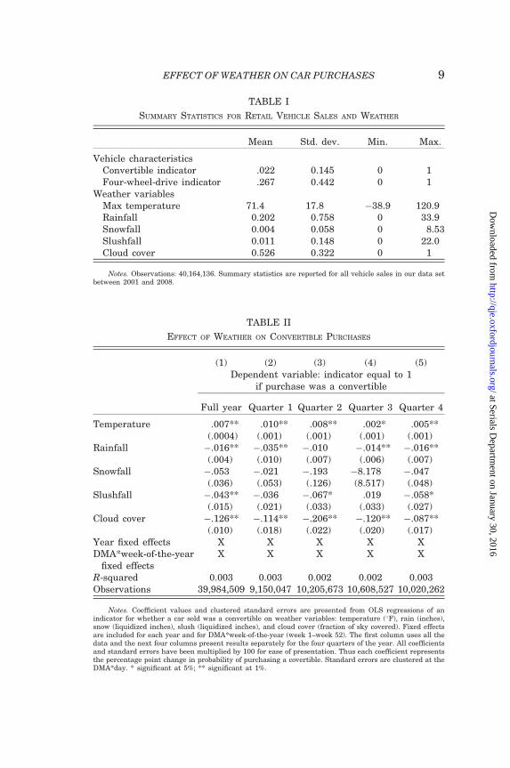
TABLE I

SUMMARY STATISTICS FOR RETAIL VEHICLE SALES AND WEATHER

Mean Std. dev. Min. Max.

Vehicle characteristicsConvertible indicator .022 0.145 0 1Four-wheel-drive indicator .267 0.442 0 1

Weather variablesMax temperature 71.4 17.8 �38.9 120.9Rainfall 0.202 0.758 0 33.9Snowfall 0.004 0.058 0 8.53Slushfall 0.011 0.148 0 22.0Cloud cover 0.526 0.322 0 1

Notes. Observations: 40,164,136. Summary statistics are reported for all vehicle sales in our data setbetween 2001 and 2008.

TABLE II

EFFECT OF WEATHER ON CONVERTIBLE PURCHASES

(1) (2) (3) (4) (5)Dependent variable: indicator equal to 1

if purchase was a convertible

Full year Quarter 1 Quarter 2 Quarter 3 Quarter 4

Temperature .007** .010** .008** .002* .005**(.0004) (.001) (.001) (.001) (.001)

Rainfall �.016** �.035** �.010 �.014** �.016**(.004) (.010) (.007) (.006) (.007)

Snowfall �.053 �.021 �.193 �8.178 �.047(.036) (.053) (.126) (8.517) (.048)

Slushfall �.043** �.036 �.067* .019 �.058*(.015) (.021) (.033) (.033) (.027)

Cloud cover �.126** �.114** �.206** �.120** �.087**(.010) (.018) (.022) (.020) (.017)

Year fixed effects X X X X XDMA*week-of-the-year

fixed effectsX X X X X

R-squared 0.003 0.003 0.002 0.002 0.003Observations 39,984,509 9,150,047 10,205,673 10,608,527 10,020,262

Notes. Coefficient values and clustered standard errors are presented from OLS regressions of anindicator for whether a car sold was a convertible on weather variables: temperature (�F), rain (inches),snow (liquidized inches), slush (liquidized inches), and cloud cover (fraction of sky covered). Fixed effectsare included for each year and for DMA*week-of-the-year (week 1–week 52). The first column uses all thedata and the next four columns present results separately for the four quarters of the year. All coefficientsand standard errors have been multiplied by 100 for ease of presentation. Thus each coefficient representsthe percentage point change in probability of purchasing a covertible. Standard errors are clustered at theDMA*day. * significant at 5%; ** significant at 1%.


at Serials Departm


Dow

nloaded from


important for convertible sales. As the sky goes from completelyclear to completely cloudy, convertible sales as a fraction of to-tal vehicles sold decreases by 0.126 percentage point. Thus,a clear sky (relative to completely overcast) increases convert-ible sales by the same amount as an increase in temperatureof 18�F.

The next four columns in Table II estimate the effect oftemperature and other weather variables on convertible salesby quarter of the year. The effect of temperature is large andstatistically significant in quarters 1, 2, and 4, but smaller inquarter 3. During quarter 3 (July, August, September), the base-line temperature is already quite warm in most areas, whichmay explain why an increase in temperature has less effect onconvertible sales than in other quarters. We find it particularlynoteworthy that high temperatures continue to have a fairlylarge effect on convertible sales in quarter 4 (October,November, December) because this is the time of year whenthe rational discounted utility of buying a convertible shouldbe the lowest. Cloud cover—which is arguably important to theperceived utility of driving a convertible no matter what time ofyear—has a large and significant effect in all quarters (includingquarter 3).

The differences across quarters in the estimated effects oftemperature on convertible purchases suggest that the effectmight be heterogeneous across the range of temperature.To assess the extent of this heterogeneity, we reestimateequation (1), replacing the linear measure of temperature withindicator variables for the 5� bin into which the daily high tem-perature falls. We use 15 indicator variables for temperatures inbins from (25–29.9�F) to (95–99.9�F). We group all days with dailyhighs of 100�F or more into a single indicator, and leave days withhigh temperatures below 25�F as our left-out group.

We report the estimated coefficients of these indicator vari-ables graphically in Figure I. For each bin, we plot the estimatecoefficient as a dot, with ‘‘whiskers’’ representing the 95% confi-dence interval around the estimated coefficient. Higher temper-atures increase the percentage of transactions that areconvertibles fairly steadily from temperatures below 25�F upuntil some point between 70�F and 80�F. At that point, theeffect flattens out, suggesting that beyond 80�F, higher tempera-tures are no longer associated with increases in the share ofvehicles sold that are convertibles.


at Serials Departm


Dow

nloaded from


0.00

0.10

0.20

0.30

0.40

0.50

0.60

0.70

25-3

0 30

-35

35-4

0 40

-45

45-5

0 50

-55

55-6

0 60

-65

65-7

0 70

-75

75-8

0 80

-85

85-9

0 90

-95

95-1

00

Mor

e th

an 1

00

The Percentage-Point Effect of Temperature (Rela�ve to Less than 25 Degrees)

High

Tem

pera

ture

Val

ue (D

egre

es F

ahre

nhei

t)

FIG

UR

EI

Fle

xib

leR

elati

onsh

ipbet

wee

nT

emp

eratu

rean

dC

onver

tible

Pu

rch

ase

s

Th

isfi

gu

rep

rovid

esth

eco

effi

cien

tvalu

esan

d95%

con

fid

ence

inte

rvals

for

the

effe

ctof

dail

yh

igh

tem

per

atu

reon

the

pro

babil

ity

ofp

urc

hasi

ng

aco

nver

tible

.E

ach

dot

plo

tsth

eco

effi

cien

tfr

omth

ere

gre

ssio

nre

por

ted

inco

lum

n(1

)of

Table

II,

bu

tw

ith

du

mm

yvari

able

sfo

r5�F

bin

sof

tem

per

atu

reu

sed

inp

lace

ofth

eli

nea

rte

mp

eratu

rete

rm.

Th

eom

itte

dte

mp

eratu

reca

tegor

yis

less

than

25�F

.


at Serials Departm


Dow

nloaded from


III.B. Effect of Weather on Four-Wheel-Drive Purchases

Although buying a convertible may seem especially attrac-tive on a warm day, it is cold and snowy days that make four-wheel-drive vehicles seem like an especially good idea. Table IIIpresents our estimates of the impact of weather variation on thepercentage of vehicles sold that are four-wheel-drives. We obtainthese estimates by substituting I(4WheelDrive), an indicator forwhether a given transaction was for a four-wheel-drive vehicle,on the left hand side of equation (1) to obtain the following esti-mation equation:

Ið4WheelDriveÞirt ¼ �0 þ b1Weatherrt þ �rT þ �Y þ �irt:ð2Þ

I(4WheelDrive) equals 1 if transaction i that occurred in DMA r onday t is for a four-wheel-drive vehicle. All other variables are as

TABLE III

EFFECT OF WEATHER ON FOUR-WHEEL-DRIVE PURCHASES

Dependent variable: indicator equal to 1if purchase was a four-wheel-drive

Full year Quarter 1 Quarter 2 Quarter 3 Quarter 4

Temperature �.032** �.038** �.018** �.029** �.038**(.001) (.002) (.003) (.004) (.003)

Rainfall .084** .119** .081** .054** .132**(.014) (.036) (.026) (.023) (.032)

Snowfall 1.81** 1.67** .72 125* 2.11**(.26) (.33) (.82) (53) (.48)

Slushfall .504** .540** .27 �.029 .769**(.077) (.110) (.22) (.167) (.166)

Cloud cover .461** .337** .512** .383** .598**(.039) (.072) (.077) (.087) (.076)

Year fixed effects X X X X XDMA*week-of-the-year

fixed effectsX X X X X

R-squared 0.086 0.086 0.074 0.084 0.097Observations 39,984,509 9,150,047 10,205,673 10,608,527 10,020,262

Notes. Coefficient values and clustered standard errors are presented from OLS regressions of anindicator for whether a car sold was a four-wheel-drive on weather variables: temperature (�F), rain(inches), snow (liquidized inches), slush (liquidized inches), and cloud cover (fraction of sky covered).Fixed effects are included for each year and for DMA*week-of-the-year (week 1–week 52). The firstcolumn uses all the data and the next four columns present results separately for the four quarters ofthe year. All coefficients and standard errors have been multiplied by 100 for ease of presentation. Thuseach coefficient represents the percentage point change in probability of purchasing a covertible. Standarderrors are clustered at the DMA*day. * significant at 5%; ** significant at 1%.


at Serials Departm


Dow

nloaded from


defined for equation (1). Our main coefficients of interest will beb1, the vector of coefficients that represent the effect of weatheron the fraction of vehicles sold in a given DMA on a given day thatare four-wheel-drive. The results are reported in Table III.

As we expected, the results we find are roughly the oppositeof what we found for convertibles. We find that colder tempera-ture values lead to more four-wheel-drive purchases. For exam-ple, on a day with temperatures that are 10�F below the averagefor that DMA and week of year, the estimated coefficient predictsthat the fraction of vehicles sold that are four-wheel-drives wouldbe 0.32 percentage point higher than otherwise. This represents a0.85% increase relative to the weighted baseline of 33.5% of ve-hicles sold with four-wheel-drive. We also find a large, positiveeffect of snow and slush on four-wheel-drive transactions. Oneinch of liquidized snow (about 10 inches of snow) leads to a 1.81percentage point increase in the percentage of total vehicles soldwith four-wheel-drive. The effects for snowfall are statisticallysignificant in quarters 1 and 4. The effect size in quarter 2 isstill reasonably large, but the standard error is much higherthan in quarters 1 and 4. The impossibly large effect estimatedfor quarter 3 and its accompanying large standard error is clearlydriven by the lack of snowfall variation that exists in the dataduring quarter 3. The effect of snowfall is slightly larger in quar-ter 4 than in quarter 1. However, the significant effect of snowfallin quarter 1 suggests that even a snow storm that occurs towardthe end of the winter season can have a powerful impact on four-wheel-drive purchase behavior.

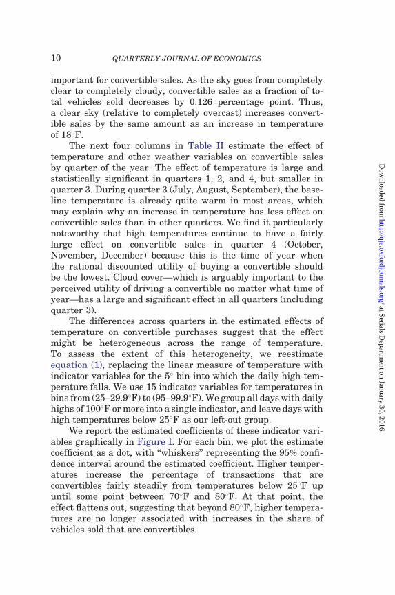
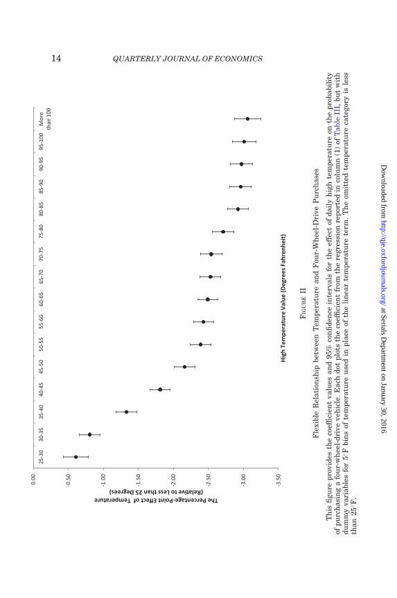
As we did when analyzing convertible purchasing, we wantto allow the effect of temperature to be nonlinear in its effect onfour-wheel-drive purchasing. We do this by reestimating equa-tion (2), replacing the linear measure of temperature with indi-cators for the same 5� bins reported in Figure I. We report theestimated coefficients on these indicator bins graphically inFigure II. As in Figure I, the dot represents the estimated coeffi-cient and the whiskers represent the 95% confidence interval.The results in Figure II indicate that changes in temperaturehave little effect on four-wheel-drive purchasing for temperaturesabove 50�F. However, for temperatures below that, each 5�F dropin temperature significantly increases the percentage of vehiclespurchased that are four-wheel-drives.

Although our estimates show that the fraction of vehiclessold that have four-wheel-drive rises in cold and snowy weather,


at Serials Departm


Dow

nloaded from


-3.5

0

-3.0

0

-2.5

0

-2.0

0

-1.5

0

-1.0

0

-0.5

0

0.00

25

-30

30-3

5 35

-40

40-4

5 45

-50

50-5

5 55

-60

60-6

5 65

-70

70-7

5 75

-80

80-8

5 85

-90

90-9

5 95

-100

M

ore

than

100

The Percentage-Point Effect of Temperature (Rela�ve to Less than 25 Degrees)

High

Tem

pera

ture

Val

ue (D

egre

es F

ahre

nhei

t)

FIG

UR

EII

Fle

xib

leR

elati

onsh

ipbet

wee

nT

emp

eratu

rean

dF

our-

Wh

eel-

Dri

ve

Pu

rch

ase

s

Th

isfi

gu

rep

rovid

esth

eco

effi

cien

tvalu

esan

d95%

con

fid

ence

inte

rvals

for

the

effe

ctof

dail

yh

igh

tem

per

atu

reon

the

pro

babil

ity

ofp

urc

hasi

ng

afo

ur-

wh

eel-

dri

ve

veh

icle

.E

ach

dot

plo

tsth

eco

effi

cien

tfr

omth

ere

gre

ssio

nre

por

ted

inco

lum

n(1

)of

Table

III,

bu

tw

ith

du

mm

yvari

able

sfo

r5�F

bin

sof

tem

per

atu

reu

sed

inp

lace

ofth

eli

nea

rte

mp

eratu

rete

rm.

Th

eom

itte

dte

mp

eratu

reca

tegor

yis

less

than

25�F

.


at Serials Departm


Dow

nloaded from


this does not necessarily mean that the total number of four-wheel-drive sales rises. One way we could obtain our results isif total vehicle sales fall in cold, snowy weather, but sales of non–four-wheel-drive vehicles fall by more than the sales of four-wheel-drive vehicles. We investigate whether this is the case byaggregating the data to the day level and regressing the log of thenumber of convertibles sold and the log of the number of four-wheel-drives sold during that day on our weather measures. Theresult show that on warm, sunny days the total number of vehi-cles sold rises, but the number of convertibles sold rises by evenmore, which is why the percentage increases. Unit sales of four-wheel-drives, however, fall on cold snowy, days, but by propor-tionally less than purchases of vehicles without four-wheel-drive.Thus, it is worth noting that the four-wheel-drive results aredriven in part by a drop in overall volume. After a snow storm,an individual who is going to purchase a four-wheel-drive vehicleappears to be more motivated go to the dealership than arebuyers of non–four-wheel-drive vehicles.

III.C. Effect of Weather on Vehicle Prices

We have shown in the previous two subsections that weatheraffects the equilibrium sales of vehicles of different types.Specifically, we have shown that the percentage of vehicles soldthat are convertibles is higher on days with warm and sunnyweather, whereas the percentage of vehicles sold that are four-wheel-drives are higher on days with cold, snowy weather. In thissection, we investigate the effect of weather on the equilibriumprices of these types of vehicles.

The most intuitive way to explain in supply-and-demandterms our estimated effects of weather on purchasing is thatweather causes a change in daily demand for different vehicletypes. If this is so, what effect would we expect weather to haveon equilibrium prices? The answer depends, of course, on theshape of the supply curve.8 In a simple supply-and-demandmodel, if the demand curve shifts out while an (upward-sloping)supply curve stays fixed, one would expect to see both higherprices and higher sales quantities.

There are several ways this simple model is not an ideal fitfor the car industry. First, from a dealer’s perspective, the supply

8. See Busse (2012) for a discussion of how different supply relationships affectthe equilibrium price and quantity that arise from changes in demand.


at Serials Departm


Dow

nloaded from


of vehicles is not upward-sloping. Dealers can order vehicles frommanufacturers at a fixed, per unit invoice price in whatever quan-tity they wish. This corresponds to horizontal marginal cost curvefor the dealer. If the dealer is selling vehicles in a competitivemarket, the effect of an increase in demand should be increasedsales, with essentially no increase in price.9

Second, a competitive price-taking market is not a very gooddescription of the retail car industry. Individual consumers nego-tiate a price for a specific vehicle with the dealer. Whether theincremental buyers who enter (or leave) the market in response toa change in weather will obtain higher prices or lower prices thanthe inframarginal buyers who are in the market at all times de-pends on the reservation prices and bargaining characteristics ofthe incremental buyers relative to the inframarginal buyers. Onemight argue that the incremental buyers must have higher res-ervation prices than buyers on average, because they are beingstrongly swayed by temporary weather conditions. Similarly, onemight argue that consumers who can buy ‘‘on impulse’’ must havehigh liquidity, and therefore likely higher incomes and higherreservation prices, than inframarginal buyers.

On the other hand, one might argue that if incrementalbuyers are buying this vehicle because of the weather (butwould not be buying it on a day with different weather), theweather must have nudged them just above their point of in-difference about buying. In this case, they might well havelower reservation prices than inframarginal buyers. Similarly,if dealers recognize which buyers are the incremental buyerswho have come into the dealership because of the temporaryweather condition, they may realize that they must offer a goodprice today or lose the sale forever, since in another few daysthe weather will change and these buyers will no longer be inthe market.10

Overall, we conclude that it is an empirical questionwhether prices for convertibles and four-wheel-drives will be

9. Dealers place orders for vehicles months in advance, so over a horizon ofseveral months, a dealer’s supply of vehicles is predetermined. However, dealerscan sell more or fewer vehicles on any given day, meaning that daily vehicle supplyis not fixed. For more on how dealer supply and inventory affects prices, seeZettelmeyer, Scott Morton, and Silva-Risso (2007).

10. We thank Glenn Ellison for suggesting this point.


at Serials Departm


Dow

nloaded from


higher on the same days that warm and sunny weather or coldand snowy weather leads to an increased sales share for thesetypes of vehicles. We estimate the effect of weather on theprices of convertibles and four-wheel-drives using the followingspecification.

Priceijrt ¼ �0 þ g1Weatherrt þ g2PurchaseTimingit

þ f ðOdometeri;g3Þ þ �rT þ �Y þ �j þ �ijrtð3Þ

Price measures the price paid in transaction i for vehicle j thatoccurred on day t in DMA r. (To make our measure of pricerepresent a customer’s total wealth outlay for the vehicle, wedefine price as the contract price for the vehicle agreed on bythe consumer and the dealer, minus any manufacturer rebatethe buyer received, plus any loss [minus any gain] the consumerreceived in negotiating a price for his or her trade-in.) Weatheris a vector containing the temperature, rainfall, snowfall, slush-fall, and cloud cover on day t in DMA r. PurchaseTiming is avector containing indicators for whether transaction i occurredduring the weekend, or at the end of the month, times in whichsalespeople may be willing to sell vehicles at a discount to hitsales volume targets. The specification also includesDMA*week-of-year (�rT), year (�Y ), and vehicle type (�j) fixedeffects. (A vehicle type is defined by the interaction of make,model, model year, trim level, doors, body type, displacement,cylinders, and transmission.) We estimate equation (3) sepa-rately for new convertibles, used convertibles, new four-wheel-drives, and used four-wheel-drives. The specifications that esti-mate the effect of weather on used vehicle prices also include alinear spline in the vehicle’s odometer with knots at 10,000-mileincrements, which allows vehicle prices to depreciate over timein a reasonably flexible way. (See Busse, Knittel, andZettelmeyer 2013 for use of a similar specification to estimateprice effects in similar data.)

Table IV reports the results of estimating equation (3).Generally speaking, we find that the effect of weather on pricesis fairly small, even when it is statistically significant. In column(1), which estimates the effect of weather on new convertibleprices, none of the weather variables have statistically significanteffects. We do not find any evidence of weather affecting thetransaction prices of convertibles. The weather coefficients, re-ported in column (1) for new convertibles and in column (2) for


at Serials Departm


Dow

nloaded from


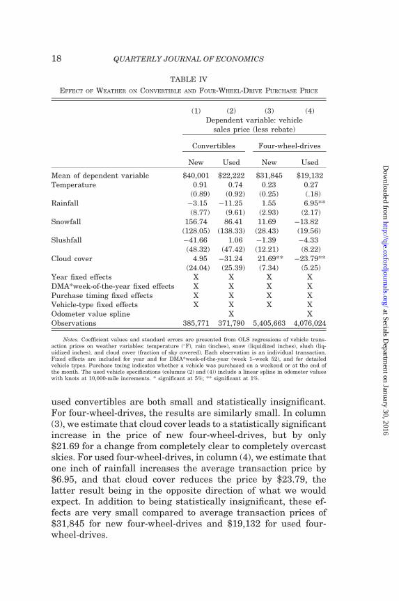
used convertibles are both small and statistically insignificant.For four-wheel-drives, the results are similarly small. In column(3), we estimate that cloud cover leads to a statistically significantincrease in the price of new four-wheel-drives, but by only$21.69 for a change from completely clear to completely overcastskies. For used four-wheel-drives, in column (4), we estimate thatone inch of rainfall increases the average transaction price by$6.95, and that cloud cover reduces the price by $23.79, thelatter result being in the opposite direction of what we wouldexpect. In addition to being statistically insignificant, these ef-fects are very small compared to average transaction prices of$31,845 for new four-wheel-drives and $19,132 for used four-wheel-drives.

TABLE IV

EFFECT OF WEATHER ON CONVERTIBLE AND FOUR-WHEEL-DRIVE PURCHASE PRICE

(1) (2) (3) (4)Dependent variable: vehicle

sales price (less rebate)

Convertibles Four-wheel-drives

New Used New Used

Mean of dependent variable $40,001 $22,222 $31,845 $19,132Temperature 0.91 0.74 0.23 0.27

(0.89) (0.92) (0.25) (.18)Rainfall �3.15 �11.25 1.55 6.95**

(8.77) (9.61) (2.93) (2.17)Snowfall 156.74 86.41 11.69 �13.82

(128.05) (138.33) (28.43) (19.56)Slushfall �41.66 1.06 �1.39 �4.33

(48.32) (47.42) (12.21) (8.22)Cloud cover 4.95 �31.24 21.69** �23.79**

(24.04) (25.39) (7.34) (5.25)Year fixed effects X X X XDMA*week-of-the-year fixed effects X X X XPurchase timing fixed effects X X X XVehicle-type fixed effects X X X XOdometer value spline X XObservations 385,771 371,790 5,405,663 4,076,024

Notes. Coefficient values and standard errors are presented from OLS regressions of vehicle trans-action prices on weather variables: temperature (�F), rain (inches), snow (liquidized inches), slush (liq-uidized inches), and cloud cover (fraction of sky covered). Each observation is an individual transaction.Fixed effects are included for year and for DMA*week-of-the-year (week 1–week 52), and for detailedvehicle types. Purchase tming indicates whether a vehicle was purchased on a weekend or at the end ofthe month. The used vehicle specifications (columns (2) and (4)) include a linear spline in odometer valueswith knots at 10,000-mile increments. * significant at 5%; ** significant at 1%.


at Serials Departm


Dow

nloaded from


IV. Rational Explanations for Weather Effects

In this section, we consider several potential explanations forthe weather effects we estimate that do not rely on any psycho-logical mechanisms. First, we consider whether our estimatedweather effects are the result of short-term intertemporal shiftsin demand. For example, it could be that consumers who havedecided to buy a convertible may wait for a nice day to actuallymake the purchase. Second, we consider whether consumers aremore likely to purchase a vehicle with a weather-related charac-teristic such as a convertible roof or four-wheel-drive on a daywhose weather enables them to test-drive the vehicle in thatweather. Third, we consider whether consumers who test-drivea convertible or a four-wheel-drive on a day with the complemen-tary weather learn thereby about their utility for the vehicle typeand that this is what drives the increased fraction of convertibleand four-wheel-drive sales on the relevant weather days.

IV.A. Shifts in Purchase Timing

Our results in Section III indicate that the fraction of vehi-cles sold on a given day that are either convertibles or four-wheel-drives is influenced by daily weather variation. One possible ex-planation for this empirical finding is that weather fluctuationsmay appear to be incrementally increasing purchases of certaintypes of vehicles, but instead just cause short-run intertemporalsubstitutions in vehicle purchasing behavior. In other words,weather shifts when, but ultimately not what, people buy. Anexample of this harvesting story is that a consumer may be inter-ested in purchasing a convertible some time in the next monthand then actually makes her purchase whenever it happens to bea nice day outside.11 Our previously noted finding that atypicallywarm weather in November can affect convertible purchases anda snow storm in February can affect four-wheel-drive purchasescasts doubt on harvesting as the sole cause of our results.However, these end-of-season purchases cannot rule out harvest-ing entirely as a contributing factor to our results.

To assess the extent to which there is short-run intertem-poral substitution of purchases with respect to daily weather

11. The fact that more convertibles are bought in spring than winter, and thereverse for four-wheel-drive vehicles, suggests that there may be harvesting inresponse to the overall seasonal pattern of the weather. However, this does notmean that harvesting happens in response to idiosyncratic weather variation.


at Serials Departm


Dow

nloaded from


fluctuations, we estimate a distributed lag model. We do so byreestimating equations (1) and (2) with 60 daily lags of eachweather variable added to the estimating equation.

IðConvertibleÞirt ¼ �0 þ a1Weatherrt

þX60

j¼1

a1;�jWeatherr;t�j þ �rT þ �Y þ �irtð4Þ

I 4WheelDriveð Þirt ¼ �0 þ b1Weatherrt

þX60

j¼1

b1;�jWeatherr;t�j þ �rT þ �Y þ �irtð5Þ

Weatherr;t�j is the vector of weather variables (temperature,rainfall, snowfall, slushfall, and cloud cover) j days before thetransaction date. a1;�j and b1;�j are vectors of coefficients thatestimate the effect of weather j days ago on day t purchases ofconvertibles and four-wheel-drives, respectively.12 By includinglagged variables, we are able to test whether having cold or hotdays leading up to the day of purchase influences how the currentweather affects behavior. For example, in the convertible sce-nario, negative coefficients on the lagged variables would be in-terpreted as evidence of harvesting via the following argument.A negative coefficient on, say, the three-day lag of temperaturewould indicate that if the weather three days ago was hot, salestoday are lower by some amount than they otherwise would havebeen. Additionally, this implies that if the weather today is hot,sales three days from now will be lower by that same amount. Wecan thus use the lag coefficients to answer the question ‘‘If theweather is hot today, how much lower will sales be in subsequentdays?’’ The one-day lag gives us an estimate for the effect of hotweather today on sales one day from now, the two-day lag esti-mates the effect of hot weather today on sales two days from now,and so on. Thus, if we add up all our lag coefficients and find thatthey equal the negative of the current period coefficient, it sug-gests that any increased sales that occur due to hot weather todayare made up entirely of sales displaced from the following

12. This specification is identical to instead regressing each of the weather var-iables on the fixed effects, obtaining residual values for each weather variable, andthen including these weather residuals and 60 days’ worth of lags of weather resid-uals in the regression.


at Serials Departm


Dow

nloaded from


60 days. More generally, the sum of the lag coefficients tells ushow much of our estimated current period effect is due to inter-temporal substitution.13

Figures III and IV present the results of this dynamicanalysis for convertible purchases estimated by equation (4).Figure III plots the estimated coefficient and confidence intervalsfor the current day’s temperature (daily lag = 0) and for 60 dailylags of temperature. Figure IV plots the coefficient and standarderrors for the current day’s cloud cover and 60 daily lags of cloudcover. The results once again show a large and significant effect ofcurrent weather on convertible purchases. The estimated coeffi-cient on the current day’s high temperature is 0.005, with a stan-dard error of 0.0006, similar to the coefficient of 0.007 reported inTable II. The coefficients on the lag variables are all small relativeto the current temperature coefficient, and all but four of the 60lag coefficients are statistically insignificant. Most important forthe question at hand, more of the coefficients are positive thannegative, especially among the most recent two or three weeks oflags. The sum of the 60 lag coefficients is 0.012; if our estimatedwarm weather effect were intertemporal shifts in sales, the coef-ficients would be expected instead to sum to the negative of thecurrent day coefficient of 0.005. We can test the null hypothesisthat the sum of the first X lags are equal to the negative of thecurrent day coefficient by imposing this as a linear restriction onthe estimation. If we do so, we reject this null hypothesis with ap-value< .001 for X equal to 7, 14, 21, 28, 45, or 60 days of lags.If anything, it appears that warm weather over the past severalweeks leads to an even higher fraction of vehicles sold today beingconvertibles.

Figure IV shows the estimated coefficients for the currentday’s cloud cover and 60 daily lags of cloud cover. In this specifi-cation, the estimated coefficient on the current day’s cloud coveris �0.125 with a standard error of 0.013, almost identical to the�0.126 reported in Table II. The sum of the 60 lag coefficients is0.199, which means that we cannot conclude that the cloud covereffects on convertible sales are not due to short-term shifts in

13. See Jacob, Lefgren, and Moretti (2007) for a similar analysis that tests forintertemporal substitution of crime using weather shocks and Deschenes andMoretti (2009) who test for intertemporal substitution of mortality using weathershocks. See these papers also for a discussion of summing up coefficient values totest for evidence of intertemporal substitution.


at Serials Departm


Dow

nloaded from


-0.0

04

-0.0

02

0.00

0

0.00

2

0.00

4

0.00

6

0.00

8

0 5

10

15

20

25

30

35

40

45

50

55

60

The Percentage-Point Effect of Temperature on Conver�ble Purchases

Daily

Lag

FIG

UR

EII

I

Dis

trib

ute

dL

ag

An

aly

sis

ofT

emp

eratu

rean

dC

onver

tible

Pu

rch

ase

s

Th

isfi

gu

rep

rovid

esth

eco

effi

cien

tvalu

esan

d95%

con

fid

ence

inte

rvals

for

the

effe

ctof

dail

yh

igh

tem

per

atu

reon

the

pro

babil

ity

ofp

urc

hasi

ng

aco

nver

tible

.E

ach

dot

plo

tsth

eco

effi

cien

tof

ala

gte

mp

eratu

revari

able

from

the

sam

ere

gre

ssio

nas

rep

orte

din

colu

mn

(1)

ofT

able

II,

bu

tw

ith

the

ad

dit

ion

of60

dail

yla

gs

ofea

chof

the

wea

ther

vari

able

s.


at Serials Departm


Dow

nloaded from


-0.2

00

-0.1

50

-0.1

00

-0.0

50

0.00

0

0.05

0

0.10

0

0 5

10

15

20

25

30

35

40

45

50

55

60

The Percentage-Point Effect of Cloud Cover on Conver�ble Purchases

Daily

Lag

FIG

UR

EIV

Dis

trib

ute

dL

ag

An

aly

sis

ofC

lou

dC

over

an

dC

onver

tible

Pu

rch

ase

s

Th

isfi

gu

rep

rovid

esth

eco

effi

cien

tvalu

esan

d95%

con

fid

ence

inte

rvals

for

the

effe

ctof

clou

dco

ver

(fra

ctio

nof

the

sky)

onth

ep

robabil

ity

ofp

urc

hasi

ng

aco

nver

tible

.E

ach

dot

plo

tsth

eco

effi

cien

tof

ala

gcl

oud

cover

vari

able

from

the

sam

ere

gre

ssio

nas

rep

orte

din

colu

mn

(1)

ofT

able

II,

bu

tw

ith

the

ad

dit

ion

of60

dail

yla

gs

ofea

chof

the

wea

ther

vari

able

s.


at Serials Departm


Dow

nloaded from


purchase timing. However, most of the positive lag coefficientsthat contribute to this result are in the longer lags. We canreject that the sum of the first X lag coefficients equal the nega-tive of the current day coefficient for X equal to 7, 14, and 21 dayswith a p-value< .001 and for 28 days with a p-value of .026. Forlonger sums of lags, we cannot reject the null hypothesis that ourresults are due to intertemporal shifts in purchase timing.However, this means that to the extent that our estimatedresult is the consequence of intertemporal shifts, it is shiftscoming mostly from more than a month ago, not shifts comingfrom the previous several weeks.

Figures V and VI provide a similar analysis for four-wheel-drive purchases. Figure V shows the current day and 60 daily lagcoefficients for temperature, and Figure VI shows them for snow-fall. The estimated coefficient of current day temperature on thefraction of vehicles sold that are four-wheel-drive is �0.015, witha standard error of 0.0027, which is somewhat smaller than the�0.032 reported in Table III. We can reject at a p-value< .001that the sum of the lagged coefficients equal the negative of thecurrent day coefficient over the 7-, 14-, 21-, 28-, 45-, or 60-dayhorizon. The lag coefficients, while not statistically significant,are more suggestive that cold weather in the two or three previ-ous weeks increases four-wheel-drive sales today.

The last set of distributed lag results is shown in Figure VI.The coefficients in this figure indicate that the current day’ssnowfall has a positive and significant effect on the fraction ofvehicles sold today that are four-wheel-drive vehicles, but sodoes snowfall on almost any of the days of the previous twoweeks. These coefficients are not consistent with shifts in pur-chase timing that would explain our empirical result fromSection III. (We can again reject at a p-value< .001 that thesum of the lagged coefficients equal the negative of the currentday coefficient over the 7-, 14-, 21-, 28-, 45-, or 60-day horizon.)Instead, the results here suggest that although a snowstormtoday has the biggest effect on sales today, it will contribute toan increased fraction of sales of four-wheel-drive vehicles foralmost two weeks.

IV.B. Test-drive Timing

One aspect of vehicle purchasing that may lead to a correla-tion between weather and vehicle purchase timing, particularly


at Serials Departm


Dow

nloaded from


-0.0

25

-0.0

20

-0.0

15

-0.0

10

-0.0

05

0.00

0

0.00

5

0.01

0

0.01

5

0.02

0

0 5

10

15

20

25

30

35

40

45

50

55

60

The Percentage-Point Effect of Temperature on 4WD Purchases

Daily

Lag

FIG

UR

EV

Dis

trib

ute

dL

ag

An

aly

sis

ofT

emp

eratu

rean

dF

our-

Wh

eel-

Dri

ve

Pu

rch

ase

s

Th

isfi

gu

rep

rovid

esth

eco

effi

cien

tvalu

esan

d95%

con

fid

ence

inte

rvals

for

the

effe

ctof

dail

yh

igh

tem

per

atu

reon

the

pro

babil

ity

ofp

urc

hasi

ng

afo

ur-

wh

eel-

dri

ve

veh

icle

.E

ach

dot

plo

tsth

eco

effi

cien

tof

ala

gte

mp

eratu

revari

able

from

the

sam

ere

gre

ssio

nas

rep

orte

din

colu

mn

(1)

ofT

able

III,

bu

tw

ith

the

ad

dit

ion

of60

dail

yla

gs

ofea

chof

the

wea

ther

vari

able

s.


at Serials Departm


Dow

nloaded from


-1.0

00

-0.5

00

0.00

0

0.50

0

1.00

0

1.50

0

2.00

0

2.50

0

0 5

10

15

20

25

30

35

40

45

50

55

60

The Percentage-Point Effect of Snowfall on 4WD Purchases

Daily

Lag

FIG

UR

EV

I

Dis

trib

ute

dL

ag

An

aly

sis

ofS

now

fall

an

dF

our-

Wh

eel-

Dri

ve

Pu

rch

ase

s

Th

isfi

gu

rep

rovid

esth

eco

effi

cien

tvalu

esan

d95%

con

fid

ence

inte

rvals

for

the

effe

ctof

dail

ysn

owfa

llon

the

pro

babil

ity

ofp

urc

hasi

ng

afo

ur-

wh

eel-

dri

ve

veh

icle

.E

ach

dot

plo

tsth

eco

effi

cien

tof

ala

gsn

owfa

llvari

able

from

the

sam

ere

gre

ssio

nas

rep

orte

din

colu

mn

(1)

ofT

able

III,

bu

tw

ith

the

ad

dit

ion

of60

dail

yla

gs

ofea

chof

the

wea

ther

vari

able

s.


at Serials Departm


Dow

nloaded from


for convertibles, is the desire of most customers to test-drive avehicle before buying. Suppose a customer is considering buying aconvertible, and she is able to forecast accurately her long-termutility from owning a convertible. Now suppose that before shebuys the convertible, she would like to be able to test out variousfeatures of it: how convenient it is to put the top up and down, howmuch wind or road noise she experiences with the top down, andso on. It is unpleasant to do such a test-drive when the weather iscold, so she waits for a warm day to go to the dealership, test-drive, and ultimately purchase the convertible. Alternatively,suppose that another customer suddenly needs a replacementvehicle, perhaps because his current vehicle has broken downand is no longer worth repairing. Suppose that a convertible isone of the vehicles he would consider purchasing, but on the dayhe needs the new vehicle it is too cold to test-drive a convertible.Unwilling to buy the convertible without being able to test out theconvertible features of the car, he buys a nonconvertible instead.

The behavior of both types of customers would lead to ahigher percentage of vehicles sold on warm days being convert-ibles relative to the percentage on cold days for reasons otherthan errors in forecasting intertemporal utility. The first type ofcustomer would lead to harvesting (customers wait until a warmweek to buy a convertible so that they can test-drive the vehicle).In the previous section, we already discussed and ruled out har-vesting effects for convertibles with regard to temperature andalso with regard to cloud cover within a four-week window.However, the second customer type is not ruled out by our dis-tributed lag model. Several pieces of evidence, however, argueagainst a test-drive learning story. For example, Figure I indi-cates that an extra degree of warm weather results in more con-vertible purchases even when the baseline temperature is in the60�F–80�F range. This is a range of temperature for which it isclearly possible for someone to test out the convertible featurescomfortably. Our results thus suggest that it is more than simplytesting the features of a car that cause warm weather to result ina higher fraction of convertibles being sold.

We can also get a sense of how important test-drive timingmight be for our results by considering the effect of cloud cover.There is no reason that a customer could not test-drive a convert-ible on a day that is cloudy, as long as it is not cold or rainy.Thus, in our regressions, which control for temperature andrain, we should not see an effect of cloud cover if the reason for


at Serials Departm


Dow

nloaded from


the correlation between temperature and convertible purchasesis test-drives. However, psychological mechanisms that causeconsumers to over-respond to current mental and emotionalstates should lead to warm, sunny days being those on whichpeople are particularly likely to buy convertibles, ratherthan warm, cloudy days. Indeed, if we examine the results inTable II, we find that unusually cloudy days have a significantnegative effect on the percentage of vehicles sold that are convert-ibles, consistent with one of several psychological mechanisms. Itis particularly noteworthy that cloudy days have a statisticallysignificant negative effect in all four quarters, and the effect ofcloudy days is largest in the third quarter, when days are gener-ally warm. This third quarter effect is especially suggestive of thefact that people buy more convertibles on warm, clear days notbecause it is more possible to test-drive them, but because itseems more attractive to own a convertible on such days.

IV.C. Consumer Learning

Another alternative hypothesis that would explain our find-ings is that customers need to test-drive a vehicle with weather-related features on a day that has the relevant weather (warmand sunny or cold and snowy) to actually learn what their utilitywill be from owning either a convertible or a four-wheel-drive insuch weather conditions. Under this hypothesis, a warm, sunnyday does not lead a customer to overestimate the utility she willget from owning a convertible; instead, it enables her to learn forthe first time how high her true utility will be from owning aconvertible in such weather states. Before considering this asan alternative hypothesis, we note that this type of extremelearning story—in which vehicle buyers cannot quite imaginewhat it would be like to own this vehicle in another state of theworld even when they have experienced that state of the worldmany times—is in itself an impediment to correctly forecastingintertemporal utility. As such, learning is a rational mechanismthat in its extreme form is very closely related to the psychologicalmechanisms we discuss in the next section.

Despite the similarity between learning as described hereand psychological biases, our data allow us to investigate some-what more direct evidence for learning as an explanation. In ourdata, we observe what trade-in, if any, customers bring whenthey buy a vehicle. This means we can observe vehicle


at Serials Departm


Dow

nloaded from


transactions by customers whom we know have owned alreadyeither a convertible or a four-wheel-drive vehicle. Previous con-vertible owners are less likely to need to learn about what it is liketo drive a convertible during a warm weather state, and similarlyfor previous four-wheel-drive owners and cold or snowy states, soevidence that idiosyncratic weather affects these consumers isparticularly strong evidence against learning as an explanation.

If we look within the subset of transactions that use a con-vertible as a trade-in, we find that approximately 25% of theseconsumers purchase another convertible whereas 75% purchasea nonconvertible vehicle. Column (1) of Table V reports the re-sults of our baseline specification if we restrict the sample to con-sumers who are trading in a convertible. Although the standarderrors are much larger due to the sample restriction, we continueto find a positive impact of temperature at the time of purchase onconvertible sales. The point estimate is about six times largerthan the point estimate in the entire sample—although thelarger estimate in percentage point terms is comparable in per-centage terms because the convertible purchase rate in thissample (25%) is so much higher.14

In column (2) of Table V, we estimate the effect of weather onconsumers who are trading in a four-wheel-drive vehicle. Overall,78% of people who trade in a four-wheel-drive vehicle purchaseanother four-wheel-drive vehicle. In column (2) we continue tofind strong and statistically significant effects of all five weathermeasures on four-wheel-drive purchases for buyers who traded ina four-wheel-drive vehicle. The estimated effects are substan-tially smaller in percentage terms than in the full sample, inlarge part because the unconditional probability of buying afour-wheel-drive vehicle is so high in this sample.15

14. The full sample results indicate that a 10�F increase in temperature in-creases the percentage of vehicles sold that are convertibles by 0.07 percentagepoint in the full sample, a 2.7% increase relative to a base percentage of 2.6%. Inthe ‘‘convertible trade-in’’ subsample, the effect is a 0.65 percentage point increase,a 2.6% increase relative to a base percentage of 25%.

15. The full sample results indicate that a 10�F decrease in temperature in-creases the percentage of vehicles sold that are four-wheel-drive by 0.32 percentagepoint in the full sample, a 0.85% increase relative to a base percentage of 33.5%. Inthe ‘‘four-wheel-drive trade-in’’ subsample, the effect is a 0.43 percentage pointincrease, a 0.55% increase relative to a base percentage of 78%. The full sampleresults indicate that one liquidized inch of snowfall increases the percentage ofvehicles sold that are four-wheel-drives by 0.81 percentage points in the fullsample, a 2.4% increase relative to a base percentage of 33.5%. In the ‘‘four-


at Serials Departm


Dow

nloaded from


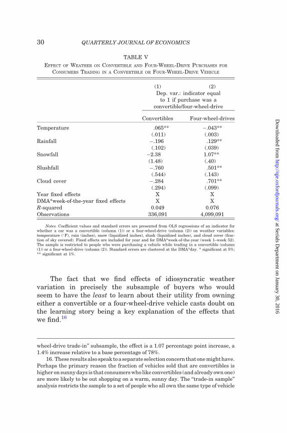
The fact that we find effects of idiosyncratic weathervariation in precisely the subsample of buyers who wouldseem to have the least to learn about their utility from owningeither a convertible or a four-wheel-drive vehicle casts doubt onthe learning story being a key explanation of the effects thatwe find.16

TABLE V

EFFECT OF WEATHER ON CONVERTIBLE AND FOUR-WHEEL-DRIVE PURCHASES FOR

CONSUMERS TRADING IN A CONVERTIBLE OR FOUR-WHEEL-DRIVE VEHICLE

(1) (2)Dep. var.: indicator equal

to 1 if purchase was aconvertible/four-wheel-drive

Convertibles Four-wheel-drives

Temperature .065** �.043**(.011) (.003)

Rainfall �.196 .129**(.102) (.039)

Snowfall �2.38 1.07**(1.48) (.40)

Slushfall �.760 .501**(.544) (.143)

Cloud cover �.284 .701**(.294) (.099)

Year fixed effects X XDMA*week-of-the-year fixed effects X XR-squared 0.049 0.076Observations 336,091 4,099,091

Notes. Coefficient values and standard errors are presented from OLS regressions of an indicator forwhether a car was a convertible (column (1)) or a four-wheel-drive (column (2)) on weather variables:temperature (�F), rain (inches), snow (liquidized inches), slush (liquidized inches), and cloud cover (frac-tion of sky covered). Fixed effects are included for year and for DMA*week-of-the-year (week 1–week 52).The sample is restricted to people who were purchasing a vehicle while trading in a convertible (column(1)) or a four-wheel-drive (column (2)). Standard errors are clustered at the DMA*day. * significant at 5%;** significant at 1%.

wheel-drive trade-in’’ subsample, the effect is a 1.07 percentage point increase, a1.4% increase relative to a base percentage of 78%.

16. These results also speak toaseparate selection concern that one might have.Perhaps the primary reason the fraction of vehicles sold that are convertibles ishigher on sunny days is that consumers who like convertibles (and already own one)are more likely to be out shopping on a warm, sunny day. The ‘‘trade-in sample’’analysis restricts the sample to a set of people who all own the same type of vehicle


at Serials Departm


Dow

nloaded from


V. Psychological Mechanisms

In the previous two sections, we provided evidence that ve-hicle consumers are highly sensitive to the weather on the day ofpurchase, effects that cannot be justified by a standard model ofconsumer choice and cannot be explained by a variety of otherrational mechanisms, such as purchase timing or learning. Inthis section we explore psychological theories that predict beingoverly sensitive to the state of the world at the time of purchase.We focus on projection bias and salience as the two most likelycandidates and separately discuss the evidence against and infavor of each of these mechanisms.17

V.A. Projection Bias

Projection bias has received significant attention in the eco-nomics and psychology literature. This bias, which is based onearlier psychological work, was formalized by Loewenstein,O’Donoghue, and Rabin (2003). In their model, Loewenstein,O’Donoghue, and Rabin assume that a person has state-depen-dent utility such that her instantaneous utility of consumption, c,in state s can be represented as uðc; sÞ. They then consider anindividual who is currently in state s0 and attempting to predicther future instantaneous utility of consumption, c, in state s; theutility prediction is denoted ~u c; s js0ð Þ. An accurate predictionwould be represented by ~u c; sjs0ð Þ ¼ uðc; sÞ.

Loewenstein, O’Donoghue, and Rabin argue that projectionbias causes agents’ predictions about future utility to be undulyinfluenced by the state they are in at the time of the prediction.Specifically, an individual exhibits projection bias if

~u c; sjs0ð Þ ¼ 1� �ð Þu c; sð Þ þ � u c; s0ð Þð Þ;ð6Þ

where � is a number between 0 and 1. If � ¼ 0, then the individualaccurately predicts her future preferences, whereas if � > 0, an

and thus helps ease this particular concern (in conjunction with some of the otherevidence that we present, such as the results from the distributed lag model).

17. Two additional psychological theories that are worth mentioning are pre-sent-biased preferences and mood effects. In an earlier version of this article, weprovided acalibration that indicated that the level of impatience required toexplainour effects are outside the range of parameter values typically found using a modelof present-biased preferences. We also find no evidence that individuals simplypurchase more expensive vehicles or sporty vehicles (e.g., coupe body style) onwarm days, which are plausible predictions of a mood effect story.


at Serials Departm


Dow

nloaded from


individual perceives her future utility to reflect a convex combi-nation of her true future utility and the utility that consumption cwould provide in her current state s0.

This simple model of projection bias can be extended easily toan intertemporal choice framework. Consider, for example, theutility that a person receives from purchasing a convertible attime tðconvtÞ and owning it until period T. Her true utility canbe represented by

Ut convt; . . . ; convTð Þ ¼XT

�¼t

��tð Þuðconv�; s�Þ;ð7Þ

where 0 � � 1 is her standard discount factor. Once again, fol-lowing Loewenstein, O’Donoghue, and Rabin (2003), a personwith projection bias perceives her intertemporal utility to be

~Ut

convt; . . . ; convTjstð Þ ¼XT

�¼t

��tð Þ ~u conv�; s�jstð Þ;ð8Þ

where ~u represents the perceived instantaneous utility describedby Equation (6).

This framework illustrates how an individual’s perceivedintertemporal utility of purchasing a convertible at time t, ~U

t,

can be overly influenced by st: Specifically, this frameworkwould predict that when st is a very good state of the world forconsuming a convertible (warm, sunny weather), an individualhas a higher perceived utility of owning the convertible thanwhen st is a bad state of the world for consuming a convertible(cold, cloudy weather).

One question that arises from this model is whether individ-uals correctly anticipate the path of states (st; . . . sT). It is possiblethat individuals are more likely to predict a greater number ofwarm-weather states in the future when the current weather iswarm relative to when the current weather is cold.18

Loewenstein, O’Donoghue, and Rabin (2003) assume that individ-uals correctly anticipate the path of states, but err when predict-ing the utility that those states combined with a givenconsumption will generate. In practice, these two errors (projec-tion bias of utility and projection bias of states) lead to similar

18. Some psychological evidence suggests that being in a hot or cold state maymake associated states of the world seem more likely in the future (see for example,Risen and Critcher 2011; Li, Johnson, and Zaval 2011).


at Serials Departm


Dow

nloaded from


incorrect predictions of future utility. Thus, it is difficult to sep-arate these different types of projection bias and our analysis doesnot attempt to do so. However, the prevalence of weather infor-mation that is available to people during the time of our study,including their own experience of local weather patterns, arguesagainst projection bias of states as the underlying mechanism. Itis much harder to find information about future utility than it isto find information about the likelihood of future weather states.

Unlike a model of present-biased preferences, which wouldrequire that the entire weather-related effect that we estimatedbe driven by consumers overweighing the value they place onconsumption in the first day or two of owning the vehicle, projec-tion bias suggests that consumers mispredict the value they willreceive from owning the convertible in every future state of theworld when the weather is different from the weather at the timeof purchase. Because the bias affects almost all periods ratherthan just one period, this model can more easily predict effectsof the size that we estimate here than can a model of present-biased preferences. While we cannot conclusively determine thatprojection bias is the sole contributing factor in the results thatwe find, our results are consistent with this psychological modelof behavior.

Conlin, O’Donoghue, and Vogelsang (2007) propose that onecan test directly for projection bias by finding evidence of con-sumers deciding ex post that a decision was a mistake.Specifically, projection bias suggests that people who make achoice in one state of the world may realize the mistake whenthe state of the world changes. Conlin, O’Donoghue, andVogelsang (2007) test for such mistakes by analyzing whethercold-weather clothing (boots, gloves, etc.) purchased by mailorder was more likely to be returned if the purchase was madeduring very cold weather. In the vehicle market, projection biasmistakes might be identified by seeing vehicles that were pur-chased on atypical weather days reappear in the market (eitheras trade-ins or as subsequent used car sales) more quickly thanvehicles that were purchased on days when the weather was sea-sonally typical. The quick return of a vehicle to the market couldindicate that the owner was not happy with the purchase he orshe made.

Unfortunately, there are at least two reasons that testing forearly returns in the vehicle market is much harder than doing sofor catalog orders. The first reason is simply a data limitation.


at Serials Departm


Dow

nloaded from


Although our data are extensive and represent a 20% sample ofall new car dealerships in the United States, we can only identify‘‘returned’’ vehicles that happen to be traded in or sold as a usedvehicle at one of the dealerships we observe. Said another way, forany vehicle whose sale we observe at some point, we have roughlya 20% chance of seeing that vehicle’s subsequent return or resaleif that transaction happens at a dealership, and no chance ofseeing it if that transaction happens person to person. Second,and perhaps more important, car dealerships do not offer the kindof ‘‘no-hassle return’’ policies that are common for catalog re-tailers. A mistake that is made when buying winter gloves canbe easily fixed with a few minutes and a little postage. However,an individual who realizes that he or she has made a mistakeafter buying a convertible cannot return it so easily. To switcha convertible for a hardtop will require the individual to sell theconvertible (likely at a loss if the vehicle is new because of therapid initial depreciation of new vehicles) and buy the hardtop(and again undergo the initial depreciation if the replacementvehicle is new). Thus, even if mistakes are being made, the mis-takes may not be large enough to merit fixing.

Despite these two concerns, we test for the impact of weatherat the time of purchase on how quickly the vehicle reappears inthe market. Of the roughly 40 million vehicles that are transactedin our data set, 2.37% of them reappear within one year as atrade-in or subsequent sale, 5.03% within two years, and 7.16%within three years.19 On average in the United States, ownerskeep their vehicles for just over five years (Polk 2010).

Our empirical strategy is to estimate whether convertiblesthat were purchased when the weather was atypically warm andfour-wheel-drive vehicles that were purchased when the weatherwas atypically cold are more likely to reappear in our data withina short time frame than vehicles purchased under more typicalweather conditions. The columns of Table VI report results forregressions in which the outcome variable is an indicator thatequals 1 for a given transaction if we observe the transacted ve-hicle reappear in our data as a trade-in or in another sales trans-action within, respectively, one, two, or three years. We controlfor DMA*week fixed effects to eliminate seasonal and geographicdifferences in how quickly vehicles are returned. Table VI shows

19. Unique identification numbers corresponding to individual vehicle identi-fication numbers are used to track vehicles over time.


at Serials Departm


Dow

nloaded from


TABLE VI

EFFECT OF WEATHER ON QUICKLY TRADING IN A VEHICLE

(1) (2) (3)Dep. var.: dummy variable if

returned within 1–3 years

1 year 2 years 3 years

Percent of cars returned in window 2.37 5.03 7.16Convertible 1.272** 2.302** 2.905**

(.019) (.030) (.042)Convertible interacted with:

Temperature .006 .017** .006(.004) (.007) (.009)

Rainfall .008 .002 �.018(.009) (.015) (.021)

Snowfall .181 �.041 �.142(.131) (.222) (.289)

Slushfall .063 .028 �.116(.053) (.094) (.131)

Cloud cover �.197 �.036 .332(.138) (.228) (.312)

Four-wheel-drive .285** .929** 1.634**(.006) (.006) (.014)

Four-wheel-drive interacted with:Temperature �.003* �.005* �.013**

(.001) (.002) (.003)Rainfall �.005 �.005 .001

(.003) (.006) (.008)Snowfall .000 .063 .004

(.035) (.058) (.076)Slushfall .002 �.019 �.048

(.016) (.028) (.038)Cloud cover .006 �.109 �.124

(.047) (.078) (.106)DMA*week fixed effects X X XR-squared 0.004 0.006 0.007Observations 35,102,062 29,665,047 23,827,418

Notes. Coefficient values and standard errors are presented from OLS regressions of a dummyvariable for whether the transacted vehicle reappears in our data set (as a trade-in car or as a used-car sale) within one, two, or three years from the date of purchase on a dummy variable for whether thetransacted vehicle was a convertible or a four-wheel-drive and an interaction between these dummies andweather variables at the time of purchase: temperature (�F), rain (inches), snow (liquidized inches), slush(liquidized inches), and cloud cover (fraction of sky covered). Each observation is at the individual vehiclelevel and DMA*week fixed effects are included. The data set is also restricted so as to eliminate alltruncation (the data eliminate the last 1–3 years of car sales in the sample, respectively). All coefficientsand standard errors have been multiplied by 100 for ease of presentation. * significant at 5%; ** signif-icant at 1%.


at Serials Departm


Dow

nloaded from


that convertibles are overall 1.272 percentage points more likelyto be returned within a year than other types of vehicles; four-wheel-drive vehicles are also more likely to be returned (by 0.285percentage point) than other types of vehicles. The positive signsof the coefficients estimated for the interaction of convertible andtemperature variables are consistent with projection bias: con-vertibles are more likely to be returned quickly when they werepurchased on days with atypically warm weather. However, thisresult is statistically significant only in column (2). The point es-timates suggest that when the weather is 10�F warmer than av-erage for that DMA and week of the year, convertibles are 0.17percentage point more likely to be returned within two years thanhardtops (a 2.3% change relative to the baseline convertiblereturn rate of 7.332%). The temperature interaction with four-wheel-drive vehicles is more consistently statistically significant,and indicates that a four-wheel-drive vehicle is more likely to bereturned within one, two, or three years if it is purchased on anatypically cold day. Overall, our results for the effect of weatheron returning vehicles, though clearly suggestive, is less strongthan our evidence for the effect on purchasing vehicles. An im-portant constraint we face is that the number of vehicles we seesold and then see reappear within our data is simply not thathigh. As a consequence, we have limited ability to identify differ-ences in the rates at which vehicles are returned under differentcircumstances.

V.B. Salience

The second psychological mechanism that we consider indetail is salience. In a consumer context, salience refers to theidea that a customer’s attention may be systematically directedtoward certain features of a product and that those features willreceive disproportionate weight in purchase decisions. The idea ofsalience is not new in the psychology literature, but it has beenformalized and received renewed attention in the past few years(see, for example, Bordalo, Gennaioli, and Shleifer 2012, 2013;Koszegi and Szeidl 2013).20

20. There have also been many recent empirical papers that find evidence ofsalience/attention. See, for example, Gabaix and Laibson (2006), Chetty, Looney,and Kroft (2009), Finkelstein (2009), Brown, Hossain, and Morgan (2010),Malmendier and Lee (2011), Lacetera, Pope, and Sydnor (2012), and Hastingsand Shapiro (2013).


at Serials Departm


Dow

nloaded from


To understand how salience could predict the effects that wefind, we consider the formalization of salience provided byBordalo, Gennaioli, and Shleifer (2013). Their model predictsthat consumers will place greater weight on product attributesthat are salient at the time of purchase. The salience of an attrib-ute is determined by how that attribute compares to the attrib-utes of the products in a consumer’s ‘‘choice context.’’ The choicecontext includes the products among which a consumer can cur-rently choose, the ‘‘choice set.’’21 In a dynamic setting, the choicecontext may also include products that the consumer expects tobe available, even if those choices aren’t currently available. Forexample, if prices have recently increased or decreased, productsat their past prices could be part of the choice context. A consumeris assumed to have a reference good whose attributes equal theaverage of the attributes in the choice context. A particular at-tribute of a good is salient (and will therefore be weighed moreheavily) when it differs by more from the reference good thanother attributes do. For example, the price of a good will bemore salient than the quality of a good if the price is more differ-ent from the price of the reference good than the quality is differ-ent from the quality of the reference good.

Hastings and Shapiro (2013) contain an application of thismodel. They consider whether salience can explain consumers’choices between gasoline grades that differ both in quality(octane rating) and price. They suppose that past prices informconsumers’ price expectations and therefore are part of con-sumers’ choice contexts when considering gasoline choices.22

Thus, if gasoline prices increase suddenly, the current prices ofgasoline will differ substantially from the reference price for gas-oline defined by the choice context, which includes the former,lower gasoline prices. This will increase the salience of prices,increasing the utility weight that consumers place on the priceattribute relative to the quality attribute of gasoline, and therebydecreasing the premium they are willing to pay for higher octanegas relative to what they were willing to pay when the overallprice levels were lower.

21. The choice context could include only a subset of choices actually available ifa consumer restricts attention to a ‘‘consideration set’’ instead of the full choice set.

22. Hastings and Shapiro use the phrase ‘‘evoked set’’ to refer to a choice con-text, referring to the set of products that are evoked in a consumer’s mind while sheis considering a particular purchase decision.


at Serials Departm


Dow

nloaded from


In Hastings and Shapiro (2013), as in many of the examplesdescribed in Bordalo, Gennaioli, and Shleifer (2013), the value ofthe attribute itself varies across contexts and causes the attrib-ute’s salience to vary (for example, gasoline prices at differentpoints in time, wine prices at stores versus restaurants, etc.). Inour context, a convertible roof does not become ‘‘more convertible’’in some contexts than others. Instead, there is another variable,weather, which varies over time and which can make the roofstyle of the car become more or less salient at different pointsin time.

For example, consider a situation in which a consumer ischoosing between one of two cars: a high-priced convertible or alow-priced sedan. In a given purchase situation, a consumer mayfind the price to be the salient feature of the vehicle or may find theroof style to be salient. On a day with especially beautiful weather,having a convertible will seem particularly attractive compared tohow it would seem on days with less nice weather. In this sense,the value of the convertible attribute today will be unusual com-pared to the value of the convertible attribute on ‘‘average’’ days,making it the salient feature, and making consumers value it morerelative to price than on days with less good weather.23

V.C. Distinguishing between salience and projection bias

As a coarse generalization, both salience and projection biaswould predict that there should be more convertibles sold on

23. How product attributes are defined is an important part of specifying thismodel. If one defines the product attribute as ‘‘roof style’’ then both a warm, sunnyday (which will make a convertible seem especially delightful to drive) and a cold,wet, blustery day (which will make a convertible seem drafty and unpleasant todrive) should make the roof style more salient, because both weather types will leadto a value of the roof type that is very different from the reference value. If theconvertible style of the roof is the generally preferred style, then when weathermakes it more salient, consumers should put more weight on roof style and be morewilling to buy a convertible whether the increased salience arose from unusuallygood weather or unusually bad weather. This is inconsistent with our results, andprobably inconsistent with most people’s intuition. To have salience explain bothincreased sales of convertibles in good weather and decreased sales of convertiblesin bad weather, we could define two product attributes that are associated with roofstyle: ‘‘enjoyableness’’ (an attribute experienced in good weather) and ‘‘draftiness’’(an attribute experienced in bad weather). Good weather would make the enjoy-ableness attribute more salient (without affecting the salience of draftiness), lead-ing to increased sales of convertibles on good weather days. Bad weather, however,would make the draftiness attribute more salient (without affecting the attribute ofenjoyableness), and would lead to decreased sales on bad weather days.


at Serials Departm


Dow

nloaded from


sunny days and more four-wheel-drives sold on snowy days.Therefore, one might well ask if there is any way to distinguishwhether salience or projection bias is a more likely explanationfor the effects we have found. One difference between the mech-anisms is that projection bias predicts that people will buy moreconvertibles when the weather is nice in an absolute sense, andsalience predicts that people will buy more convertibles when theweather is unusually nice relative to some benchmark (since it isin comparison to the average that makes an attribute salient).Said another way, projection bias predicts something about theeffect of weather ‘‘levels’’ and salience predicts something aboutthe effect of weather ‘‘differences’’ or ‘‘surprises.’’

Whether this distinction enables us to tease apart thesetwo potential mechanisms depends on what kinds of weather‘‘surprises’’ one thinks are relevant for salience. One definitionof a weather surprise would be weather that differs from the av-erage weather at that time of year. In other words, consumers aresurprised when the weather is different from the expectation theyhave formed based on their experience of weather in past years.Another definition of a weather surprise would be weather thatdiffers from what the weather has been recently, in the last fewdays or weeks, for example. In this case, consumers would besurprised when the weather changes from what it has been re-cently. In terms of the formal model of Bordalo, Gennaioli, andShleifer, the distinction is whether the reference good is ‘‘drivinga convertible in weather that is typical for this time of year’’ orwhether the reference good is ‘‘driving a convertible in theweather experienced over the last few days or weeks.’’

We cannot distinguish between projection bias and salienceunder the ‘‘surprise relative to expectations’’ interpretation. Thereason for this has been described already. Summarizing briefly,weather follows a seasonal trend, which means that there is avery plausible discounted utility explanation for a correlation be-tween weather and car sales. Therefore, we would not want toattribute a correlation in the seasonal pattern of weather and carsales to an intertemporal bias. The only empirical effect that wecould attribute to a psychological bias (either projection bias orsalience) is an effect of atypical weather on car sales (since atemporary weather fluctuation shouldn’t affect the discountedutility of owning a long-lived durable good). Unfortunately, thecorrelation of atypical weather with car sales would be predicted


at Serials Departm


Dow

nloaded from


by both mechanisms, and therefore doesn’t enable us to distin-guish between the two.

In contrast, under the ‘‘weather surprise relative to recent’’interpretation of when particular attributes of a car should besalient, we may be able to distinguish between the two mecha-nisms. In the language of Bordalo, Gennaioli, and Shleifer, sup-pose that the ‘‘choice set’’ part of a consumer’s choice contextincludes both convertibles and nonconvertibles on the day of pur-chase (with its associated weather) and the ‘‘expectations’’ part ofthe choice context includes the same vehicles in the days leadingup to the actual purchase (which might have had differentweather states). If this is the case, then the roof style of a carshould be particularly salient when the weather on the date ofpurchase is not only nice but nice relative to the weather in thedays leading up to the purchase. For example, if the weather wasvery cool and cloudy in the week leading up to the purchase, thenwarm and sunny weather on the day of purchase makes the con-vertible feature particularly unusual relative to the referencegood in the choice context. Projection bias, on the other hand,does not predict that convertible sales would be higher on a goodweather day that follows a string of bad weather days than on agood weather day that follows a string of other good weather days.

This prediction was tested in Section IV.A when we providedresults from a distributed lag model.24 For convertibles, we foundthat conditional on the weather at the time of purchase, colderweather in the days leading up to the purchase did not lead toincreased sales relative to warmer weather in the days leading upto the purchase. Although this finding goes against the predictionthe salience model would make if the previous days’ weather iswhat the choice context expectation is based on, it is also possiblethat buying a car a few days earlier is not in a consumers’ choicecontext (or maybe it is only a small part of the overall choicecontext that consumers use, making this effect hard to identify).

A prediction that could differ between a model of projectionbias and salience is as follows. When the weather is extremelycold (e.g., 25�F), it could be the case that increasing the temper-ature by a small amount (e.g., to 35�F) would have no impact onthe current utility associated with owning and driving a convert-ible. Thus, a model of projection bias would not predict that a

24. This prediction of a model of salience provides the same prediction as inter-temporal substitution of car purchases.


at Serials Departm


Dow

nloaded from


movement of temperature from 25�F to 35�F would have anyimpact on convertible sales. However, moving from 25�F to35�F could change the salience placed on a convertible featurewhen making a car purchase even if current utility doesn’tchange. A model of salience could therefore result in a higherfraction of convertibles purchased as the temperature increasedfrom 25�F to 35�F. Based on Figure I, we find that car sales arepositively correlated with temperature even at very low temper-ature levels. This finding could be seen as evidence for saliencerather than projection bias if one believes that differences in tem-peratures within the low range of temperatures will not affect theperceived utility of driving a convertible.

Overall, it is very difficult to distinguish between projectionbias and salience in this domain; our primary results are consis-tent with either model.

VI. Conclusion

Many of the most important decisions that we make in lifeare those with long-term implications. Our ability to make thesedecisions well depends in part on our ability to forecast accuratelyour intertemporal utility. In this article, we have examined pur-chasing behavior in the car market and found evidence that con-sumers are affected by projection bias or salience, limiting theirability to make the decision that will maximize their long-termutility. We argue that our results imply that behavioral biasescan have important implications for large-stakes markets andthat these biases merit additional study and attention.

From a policy perspective, our results suggest that con-sumers would benefit from laws designed to help them betterevaluate their decisions. For example, laws that allow consumersa ‘‘cooling-off period’’ for durable goods or goods for which con-sumers sign extended contracts may provide significant benefitsto consumers (Lowenstein, O’Donoghue, and Rabin, 2003). Suchlaws could also provide incentives for sellers to help buyers be in a‘‘cool’’ state before an important transaction or contract is made.25

The Federal Trade Commission has an explicit ‘‘Cooling-Off Rule’’that applies to situations when ‘‘[you] buy an item in your home

25. See Camerer et al. (2003) for an extended discussion about cooling-off pe-riods and their potential applications in settings where people make suboptimalchoices.


at Serials Departm


Dow

nloaded from


or at a location that is not the seller’s permanent place ofbusiness.’’26 This rule was made specifically to deal with high-pressure sale situations such as door-to-door sales. The FederalTrade Commission’s Cooling-Off Rule does not apply to automo-bile sales even though there clearly can be high-pressure salesituations for this important durable good. Although our resultssuggest that some consumers might benefit from an opportunityto reverse a decision once they have cooled off, applying a cooling-off rule to vehicle purchases would provide other consumers anopportunity to game the system by ‘‘buying’’ a new convertible atthe beginning of a holiday weekend and returning it after a fewdays, claiming to have had a change of heart.

Despite showing that intertemporal behavioral biases canimpact an important consumer durable good market, there aremany questions about the behavioral bias we have documentedthat are left unanswered and that future research may be able toaddress. For example, it is unclear how easy it is to ‘‘de-bias’’consumers. It is possible that simply providing consumers withinformation about how intertemporal choices can be influencedby behavioral biases, or asking them to imagine how they will feelabout their purchase in a different state of the world, could lead toimproved decision making. Another extension of our researchthat would be particularly useful would be to study behavioralbiases in intertemporal choice in various other important empir-ical contexts such as the decision of a couple to have a baby,whether to get married, which house to buy, or whether toaccept a given job offer. Studying intertemporal choice bias inother important settings such as these may offer additional em-pirical tests that could shed light on the relative strength andimportance of the underlying behavioral mechanisms, such asprojection bias and salience, that have been hypothesized in theliterature in these different choice contexts.

Northwestern University and NBER

University of Chicago and NBER

Brigham Young University

University of California, Riverside

26. More information on the Federal Trade Commission’s Cooling-Off Rule canbe found oat: http://www.ftc.gov/bcp/edu/pubs/consumer/products/pro03.shtm.


at Serials Departm


Dow

nloaded from

http://www.ftc.gov/bcp/edu/pubs/consumer/products/pro03.shtm


Supplementary Material

An Online Appendix for this article can be found at QJEonline (qje.oxfordjournals.org).

References

Bordalo, Pedro, Nicola Gennaioli, and Andrei Shleifer, ‘‘Salience Theory of Choiceunder Risk,’’ Quarterly Journal of Economics, 127 (2012), 1243–1285.

———, ‘‘Salience and Consumer Choice,’’ Journal of Political Economy, 121(2013), 803–843.

Brown, Jennifer, Tanjim Hossain, and John Morgan, ‘‘Shrouded Attributes andInformation Suppression: Evidence from the Field,’’ Quaterly Journal ofEconomics, 125 (2010), 859–876.

Busse, M., ‘‘When Supply and Demand Just Won’t Do: Using the Equilibrium Locusto Think about Comparative Statics,’’ (Mimeo, Northwestern University, 2012).

Busse, M., C. Knittel, and F. Zettelmeyer, ‘‘Are Consumers Myopic?: Evidencefrom New and Used Car Purchases,’’ American Economic Review, 103(2013), 220–256.

Busse, M., D. Simester, and F. Zettelmeyer, ‘‘ ‘The Best Price You’ll Ever Get’: The2005 Employee Discount Pricing Promotions in the U.S. AutomobileIndustry,’’ Marketing Science, 29 (2010), 268–290.

Camerer, C., S. Issacharoff, G. Loewenstein, T. O’Donoghue, and M. Rabin,‘‘Regulation for Conservatives: Behavioral Economics and the Case for‘Asymmetric Paternalism’,’’ University of Pennsylvania Law Review, 151(2003), 1211–1254.

Chetty, Raj, Adam Looney, and Kory Kroft, ‘‘Salience and Taxation: Theory andEvidence,’’ American Economic Review, 99 (2009), 1145–1177.

Conlin, M., T. O’Donoghue, and T. Vogelsang, ‘‘Projection Bias in Catalog Orders,’’American Economic Review, 97 (2007), 1217–1249.

Deschenes, O., and E. Moretti, ‘‘Extreme Weather Events, Mortality, andMigration,’’ Review of Economics and Statistics, 91 (2009), 659–681.

DellaVigna, S., ‘‘Psychology and Economics: Evidence from the Field,’’ Journal ofEconomic Literature, 47 (2009), 315–372.

Finkelstein, Amy, ‘‘E-ZTax: Tax Salience and Tax Rates,’’ Quarterly Journal ofEconomics, 124 (2009), 969–1010.

Gabaix, Xavier, and David Laibson, ‘‘Shrouded Attributes, Consumer Myopia, andInformation Suppression in Competitive Market,’’ Quarterly Journal ofEconomics, 121 (2006), 505–540.

Hastings, J., and J. Shapiro, ‘‘Fungibility and Consumer Choice: Evidence fromCommodity Price Shocks,’’ Quarterly Journal of Economics, 128 (2013),1449–1498.

Jacob, B., L. Lefgren, and E. Moretti, ‘‘The Dynamics of Criminal Behavior:Evidence from Weather Shocks,’’ Journal of Human Resources, 42 (2007),489–527.

Koszegi, Botond, and Adam Szeidl, ‘‘A Model of Focusing in Economic Choice,’’Quarterly Journal of Economics, 128 (2013), 53–107.

Lacetera, Nicola, Devin Pope, and Justin Sydnor, ‘‘Heuristic Thinking andLimited Attention in the Car Market,’’ American Economic Review, 102(2012), 2206–2236.

Laibson, D., ‘‘Golden Eggs and Hyperbolic Discounting,’’ Quarterly Journal ofEconomics, 112 (1997), 443–477.

Li, Y., E. Johnson, and L. Zaval, ‘‘Local Warming: Daily Temperature ChangeInfluences Belief in Global Warming,’’ Psychological Science, 22 (2011),454–459.

Loewenstein, G., T. O’Donoghue, and M. Rabin, ‘‘Projection Bias in PredictingFuture Utility,’’ Quarterly Journal of Economics, 118 (2003), 1209–1248.

Malmendier, Ulrike, and Young Han Lee, ‘‘The Bidder’s Curse,’’ AmericanEconomic Review, 101 (2011), 749–787.

O’Donoghue, T., and M. Rabin, ‘‘Doing It Now or Later,’’ American EconomicReview, 89 (1999), 103–124.


at Serials Departm


Dow

nloaded from



Polk, ‘‘Consumers Continuing to Hold onto Vehicles Longer,’’ November 3, 2010,available at https://www.polk.com/company/news/consumers_continuing_to_hold_onto_vehicles_longer_according_to_polk.

Risen, J., and C. Critcher, ‘‘Visceral Fit: While in a Visceral State, AssociatedStates of the World Seem More Likely,’’ Journal of Personality and SocialPsychology, 100 (2011), 777–793.

Zettelmeyer, F., F. Scott Morton, and J. Silva-Risso, ‘‘Scarcity Rents in CarRetailing: Evidence from Inventory Fluctuations at Dealerships,’’ Mimeo,Northwestern University, 2007.


at Serials Departm


Dow

nloaded from

https://www.polk.com/company/news/consumers_continuing_to_hold_onto_vehicles_longer_according_to_polk

https://www.polk.com/company/news/consumers_continuing_to_hold_onto_vehicles_longer_according_to_polk


i. introduction - booth school of...

Documents