i introduction - university of...

Progress in Physical Geography 29, 4 (2005) pp. 449–474

© 2005 Edward Arnold (Publishers) Ltd 10.1191/0309133305pp455ra

I IntroductionEnvironmental management and conservationagendas commonly include requirements formapping and monitoring wildlife habitat for thepurpose of estimating population sizes, identi-fying critical habitat, and predicting theimpacts of environmental change. While occa-sionally conducted over small geographic areas(e.g., Radeloff et al., 1999; Lauver et al., 2002)these initiatives commonly require regional, or,increasingly, global perspectives that defy tra-ditional field-based techniques (e.g., Skidmoreand Gauld, 1996; Corsi et al., 1999; Osborne

et al., 2001). In light of these challenges,remote sensing has often been identified as akey data source for supporting habitat mappingand other large-area ecological applications(Graetz, 1990; Roughgarden et al., 1991;Wickland, 1991). The promise of the technologylies in its potential to deliver informationabout key ecological drivers over large areaswith regular temporal revisit periods. Thesesentiments are reflected in the growingnumber of ‘integrated’ remote sensing-ecology studies in the literature (e.g., Hinesand Franklin, 1997; Carroll et al., 1999;

Remote sensing for large-areahabitat mapping

Gregory J. McDermid1, Steven E. Franklin2

and Ellsworth F. LeDrew3

1Department of Geography, University of Calgary, Calgary,AB T2N 1N4, Canada2Department of Geography, University of Saskatchewan, Saskatoon,SK S7N 5A5, Canada3Department of Geography, University of Waterloo, Waterloo,ON N2L 3G1, Canada

Abstract: Remote sensing has long been identified as a technology capable of supporting thedevelopment of wildlife habitat maps over large areas. However, progress has been constrained byunderdeveloped linkages between resource managers with extensive knowledge of ecology andremote sensing scientists with backgrounds in geography. This article attempts to traverse that gapby (i) clarifying the imprecise and commonly misunderstood concept of ‘habitat’, (ii) exploringthe recent use of remote sensing in previous habitat-mapping exercises, (iii) reviewing theremote sensing toolset developed for extracting information from optical satellite imagery, and(iv) outlining a framework for linking ecological information needs with remote sensing techniques.

Key words: habitat mapping, remote sensing, scene models, vegetation structure.

450 Remote sensing for large-area habitat mapping

Kobler and Adamic, 1999; Skidmore, 2002).However, the technology remains a ‘blunttool’ (Plummer, 2000) requiring a significantamount of multidisciplinary research andjoint understanding in order to reach its fullpotential.

Multidisciplinary approaches to scienceand management are tremendously appeal-ing, because they bring together individualswith different experience and backgroundswhose constructive exchange of ideas havethe potential to generate novel solutions.However, such projects are often challengingin that people entering new disciplines oftendo not possess the necessary backgroundknowledge, and lack the ability to communi-cate effectively with their new peers. Such isclearly the case with the remote sensing-ecology interface, where significant gaps ofunderstanding exist between the ‘tools’experts – practitioners of remote sensing,GIS, and other spatial techniques – andecologists. Plummer (2000) lamented theissue in the context of ecological processmodels, but a wider survey of the literaturereveals this to be a common pattern. In theirreview of remote sensing protocols used inthe national Gap Analysis Program, Eve andMerchant (1998) offered the following adviceto new projects just getting under way withtheir ecological mapping: ‘Brace yourself andgood luck!’

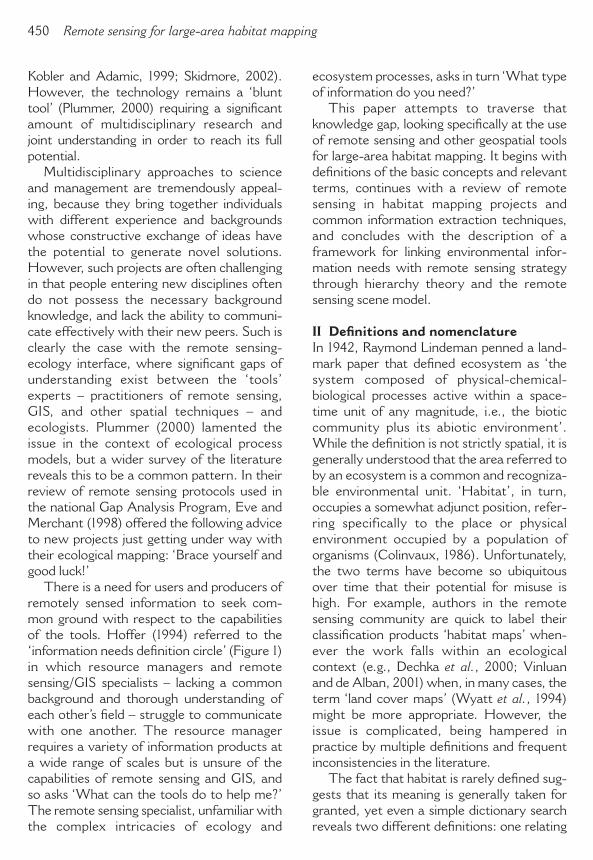
There is a need for users and producers ofremotely sensed information to seek com-mon ground with respect to the capabilitiesof the tools. Hoffer (1994) referred to the‘information needs definition circle’ (Figure 1)in which resource managers and remotesensing/GIS specialists – lacking a commonbackground and thorough understanding ofeach other’s field – struggle to communicatewith one another. The resource managerrequires a variety of information products ata wide range of scales but is unsure of thecapabilities of remote sensing and GIS, andso asks ‘What can the tools do to help me?’The remote sensing specialist, unfamiliar withthe complex intricacies of ecology and

ecosystem processes, asks in turn ‘What typeof information do you need?’

This paper attempts to traverse thatknowledge gap, looking specifically at the useof remote sensing and other geospatial toolsfor large-area habitat mapping. It begins withdefinitions of the basic concepts and relevantterms, continues with a review of remotesensing in habitat mapping projects andcommon information extraction techniques,and concludes with the description of aframework for linking environmental infor-mation needs with remote sensing strategythrough hierarchy theory and the remotesensing scene model.

II Definitions and nomenclatureIn 1942, Raymond Lindeman penned a land-mark paper that defined ecosystem as ‘thesystem composed of physical-chemical-biological processes active within a space-time unit of any magnitude, i.e., the bioticcommunity plus its abiotic environment’.While the definition is not strictly spatial, it isgenerally understood that the area referred toby an ecosystem is a common and recogniza-ble environmental unit. ‘Habitat’, in turn,occupies a somewhat adjunct position, refer-ring specifically to the place or physicalenvironment occupied by a population oforganisms (Colinvaux, 1986). Unfortunately,the two terms have become so ubiquitousover time that their potential for misuse ishigh. For example, authors in the remotesensing community are quick to label theirclassification products ‘habitat maps’ when-ever the work falls within an ecologicalcontext (e.g., Dechka et al., 2000; Vinluanand de Alban, 2001) when, in many cases, theterm ‘land cover maps’ (Wyatt et al., 1994)might be more appropriate. However, theissue is complicated, being hampered inpractice by multiple definitions and frequentinconsistencies in the literature.

The fact that habitat is rarely defined sug-gests that its meaning is generally taken forgranted, yet even a simple dictionary searchreveals two different definitions: one relating

Gregory J. McDermid et al. 451

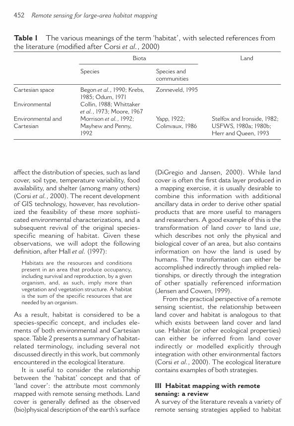
to location – the place where a species iscommonly found – and the other relating tocondition – the type of environment in whichan organism normally occurs (Merriam-Webster, 1998). While Morrison et al. (1992)noted this initial dichotomy, a survey of theliterature reveals an even more complicatedsituation. Corsi et al. (2000) partitioned thevarious meanings of habitat into a nine-cellmatrix (Table 1), showing that the term canrefer to a distinct species or community (e.g.,grizzly bear habitat), or a land attribute withno relation to biota (e.g., riparian habitat).Specific definitions can also include elementsof Cartesian space, environmental space, orboth. The situation is further complicated byfrequent examples of ambiguity in the litera-ture; sometimes within the same publication.For example, Lehmkuhl and Raphael (1993)used the terms ‘old-forest habitat’ and ‘owlhabitat’ simultaneously in a paper aboutnorthern spotted owls in the OlympicPeninsula. All of the above contributes tomisunderstanding amongs multidisciplinarycolleagues, and prompted Hall et al. (1997) toissue a plea for standard terminology.

Corsi et al. (2000) speculated that theorigin of the word habitat – Latin for habitare,or ‘to dwell’ – reflects its initial purpose as a

term to describe the environment a specieslives in. Its gradual transformation into moreof a land-based concept is likely related to theemergence of widespread habitat andbiodiversity mapping, in which individualmaps for every species are virtually impossibleto produce (Kerr, 1986). The term ‘habitattype’, defined as a mappable unit of landhomogeneous with respect to vegetation andenvironmental factors (Jones, 1986), is a likelyproduct of this trend. In retrospect, thiscontext likely forms the basis of many remotesensing ‘habitat maps’, and subsequentconfusion over the use of the term.

Considered carefully, the value of habitattype maps is based on the assumption that anarea exhibiting similar vegetation cover is alsolikely to contain homogeneous conditionswith respect to other environmental gradi-ents. However, it seems unlikely that thevariation of factors affecting the distributionof all species is completely interdependent,which would lead one to conclude that habi-tat types are not truly homogeneous. It alsoseems reasonable to speculate that the focuson habitat types as an ecological mappingunit may have arisen from an early lack ofsophisticated spatial tools capable of portray-ing the many environmental factors that

Figure 1 The information needs definition circleSource: Adapted from Hoffer (1994).

affect the distribution of species, such as landcover, soil type, temperature variability, foodavailability, and shelter (among many others)(Corsi et al., 2000). The recent developmentof GIS technology, however, has revolution-ized the feasibility of these more sophisti-cated environmental characterizations, and asubsequent revival of the original species-specific meaning of habitat. Given theseobservations, we will adopt the followingdefinition, after Hall et al. (1997):

Habitats are the resources and conditionspresent in an area that produce occupancy,including survival and reproduction, by a givenorganism, and, as such, imply more thanvegetation and vegetation structure. A habitatis the sum of the specific resources that areneeded by an organism.

As a result, habitat is considered to be aspecies-specific concept, and includes ele-ments of both environmental and Cartesianspace. Table 2 presents a summary of habitat-related terminology, including several notdiscussed directly in this work, but commonlyencountered in the ecological literature.

It is useful to consider the relationshipbetween the ‘habitat’ concept and that of‘land cover’: the attribute most commonlymapped with remote sensing methods. Landcover is generally defined as the observed(bio)physical description of the earth’s surface

(DiGregio and Jansen, 2000). While landcover is often the first data layer produced ina mapping exercise, it is usually desirable tocombine this information with additionalancillary data in order to derive other spatialproducts that are more useful to managersand researchers. A good example of this is thetransformation of land cover to land use,which describes not only the physical andbiological cover of an area, but also containsinformation on how the land is used byhumans. The transformation can either beaccomplished indirectly through implied rela-tionships, or directly through the integrationof other spatially referenced information(Jensen and Cowen, 1999).

From the practical perspective of a remotesensing scientist, the relationship betweenland cover and habitat is analogous to thatwhich exists between land cover and landuse. Habitat (or other ecological properties)can either be inferred from land coverindirectly or modelled explicitly throughintegration with other environmental factors(Corsi et al., 2000). The ecological literaturecontains examples of both strategies.

III Habitat mapping with remotesensing: a reviewA survey of the literature reveals a variety ofremote sensing strategies applied to habitat


Table 1 The various meanings of the term ‘habitat’, with selected references fromthe literature (modified after Corsi et al., 2000)

Biota Land

Species Species and communities

Cartesian space Begon et al., 1990; Krebs, Zonneveld, 19951985; Odum, 1971

Environmental Collin, 1988; Whittakeret al., 1973; Moore, 1967

Environmental and Morrison et al., 1992; Yapp, 1922; Stelfox and Ironside, 1982; Cartesian Mayhew and Penny, Colinvaux, 1986 USFWS, 1980a; 1980b;

1992 Herr and Queen, 1993

mapping projects spanning a wide range ofspatial scales (Table 3). Manual interpretationof aerial photographs has often beenemployed by studies that involve species withlimited ranges and/or the analysis of relativelysmall areas. For example, Palma et al. (1999)used manual interpretation of 1:10 000 photo-graphy to extract a variety of environmentalvariables including landcover, landcoverdiversity, road density, and drainage densityto characterize the habitat immediately sur-rounding confirmed sightings of Iberian lynxin the western Algarve region of Portugal.Lauver et al. (2002) used 1:12 000 digitalorthophotos to map detailed environmentalvariables such as tree density and hedgerowlocation in order to assess loggerhead shrikehabitat suitability over a 40 000 ha study areain Kansas. In both these cases, remote sensingserved primarily as a complement to fieldsurveys, and made use of skilled interpretersto generate detailed, high-quality informa-tion. Unfortunately, the labour-intensivenature of such manual procedures tends tolimit the range over which this type of analy-sis can be conducted.

Researchers faced with larger study areashave typically turned to digital processing ofmedium-spatial-resolution satellite imagerysuch as Landsat Multispectral Scanner(MSS), Thematic Mapper (TM), orEnhanced Thematic Mapper Plus (ETM�)for more efficient acquisition of environmen-tal information. Landcover, in particular, playsa prominent role in most regional-scale habi-tat studies. McClain and Porter (2000), forexample, used TM-derived landcover maps toevaluate white-tailed deer habitat in theAdirondacks of New York. A second study byNielsen et al. (2003) used resource selectionfunctions to link grizzly bear location data to a landcover map covering more than10 000 km2 in the foothills of Alberta,Canada. However, while landcover mapsmay contain useful predictive power, they areoften not capable of revealing the underlyingmechanisms and dynamic nature of complexnatural landscapes.

Several researchers have attempted tosupplement basic landcover information withfragmentation metrics, topographic meas-ures, and vegetation indices, among others.


Table 2 Habitat terminology (modified after Krausman, 1999)

Term Definition

Habitat The sum and location of the specific resources needed by an organism for survival and reproduction

Habitat type A mappable unit of land considered homogeneous with respect to vegetation and environmental factors

Habitat use The way an organism uses the physical and biological resources in a habitatHabitat selection A series of innate and learned behavioural decisions made by an animal about

what habitat it would useHabitat preference The consequences of habitat selectionHabitat availability The accessibility and procurability of the physical and biological components of a

habitat Habitat suitability The ability of the habitat to sustain life and support population growthHabitat quality The ability of the environment to provide conditions appropriate for individual and

population persistenceCritical habitat A legal term describing the physical or biological features essential to the

conservation of a species, which may require special managementconsiderations or protection

For example, Danks and Klein (2002) used thetopographic variables elevation, slope, aspect,and ruggedness to develop predictive modelsof muskoxen habitat in northern Alaska.Other studies have demonstrated the value offragmentation metrics as indicators of habitatstructure. For example, Hargis et al. (1999)employed a suite of spatial statistics toinvestigate the effects of forest fragmentationon American martens in the Uinta Mountainsof Utah. In a later study, Hansen et al. (2001)explored the spatial effects of timber harvest-ing on woodland caribou habitat in south-eastern British Columbia, Canada. Whilethese approaches seem capable of summariz-ing complex spatial habitat requirements, thechallenge involves selecting the correctmetrics and identifying the appropriate scaleof observation.

The challenge of balancing the needfor detailed information with the cost and

complexities involved with producing suchinformation increases directly with study areasize. Habitat projects operating at thenational and continental level are often forcedby practical reasons to use more generalizedvariables from coarse-resolution satellitedata. For example, Wallin et al. (1992) usedthe Normalized Difference Vegetation Index(NDVI) of 4 km AVHRR imagery in theiranalysis of breeding habitat for the red-billedquelea in sub-Saharan Africa. The authorshypothesized that NDVI would be capable ofproviding a reasonable index of more detailed(and unavailable) measures such as vegeta-tion condition and food availability.

The growing demand for large areaenvironmental information is reflected by thenumerous large-area data initiatives, includinglandcover maps of the United States(Loveland et al., 1991), Canada (NationalResources Canada, 1995), and the world


Table 3 Literature examples showing the range of scales and remotesensing-derived variables used in previous habitat mapping projects

Local Regional National/Continental

Land cover Palma et al., 1999; Hines and Franklin, 1997; Osborne et al., 2001Radeloff et al., 1999; Roseberry, 1998; Kurki et al.,Lauver et al., 2002 1998; Carroll et al., 1999;

Smith et al., 1998; McClain and Porter, 2000; García Borboroglu et al., 2002; Ciarniello et al., 2002; Danks and Klein, 2002; Norris et al., 2002; Rushton et al., 1997; Woolf et al., 2002; Nielsen et al., 2003

Topography Palma et al., 1999 Ciarniello et al., 2002; Danks Osborne et al., 2001and Klein, 2002; Woolf et al., 2002; Nielsen et al., 2003

Fragmentation Radeloff et al., 1999; Hines and Franklin, 1997; Palma et al., 1999 Roseberry, 1998; Kurki et al.,

1998; Hargis et al., 1999; Woolf et al., 2002

Vegetation Verlinden and Masogo, Wallin et al., 1992greenness/phenology 1997; Ciarniello et al., 2002

Vegetation structure Radeloff et al., 1999; Hines and Franklin, 1997; Lauver et al., 2002 Carroll et al., 1999

(Hansen et al., 2000); the Pathfinder (Maiden,1994; James and Kalluri, 1994) and MODIS(Justice and Townshend, 2002) data sets; andthe National Gap Analysis Program (Scott et al., 1993). However, these data are likely tolack the spatial grain and environmental detailnecessary for most habitat-mapping projects.

At the leading edge of the discipline arestudies that have attempted to incorporatedetailed vegetation attributes such as taxon-omy, age, and structure derived from widelyavailable satellite imagery. The work byCarroll et al. (1999) stands out with its use ofsophisticated TM-derived estimates ofcanopy closure, tree size, and percent coniferin a study of fisher habitat in the Klamathregion of Oregon and California. In similarworks, Hines and Franklin (1997) andFranklin and Stephenson (1996) demon-strated the value of a high-quality, regional-scale (2 million ha) vegetation database in theSan Bernardino Mountains of southernCalifornia that included spatially detailedinformation on forest cover (landcover, frag-mentation) and canopy structure (canopycoverage, tree crown size) with an analysis ofhabitat quality for the California spotted owl.

While obviously expensive and difficult toproduce, large-area vegetation databaseswith at least moderate levels of structuraland taxonomic detail are likely required formost large-area habitat studies. Deriving suchdatabases is a tremendous challenge thatrequires the intelligent coupling of ecologicaltheory and remote sensing technique.

IV Remote sensing informationextraction strategiesThe application of remote sensing techniquesto large-area habitat projects is often hinderedby the relative immaturity of the RS/GISdiscipline. Researchers both inside and outsidethe field tend to forget that we have only beenworking with earth-observing satellites forabout 30 years, and that truly large-areaprojects (those combining information fromtwo or more adjacent scenes) have only beenwidely attempted within the past decade.

Several works (e.g., Meyer and Werth,1990; Mladenoff and Host, 1994) havecriticized the ‘overselling’ of Landsat data,citing the inconsistent delineation of speciescomposition and detailed vegetation struc-ture, among other issues. In response, somespecialists have pointed to the vast technicalgains over early MSS instruments (Hoffer,1994), improved algorithms (e.g., Bolstad andLillesand, 1992; Cohen et al., 1995; 2003),and the introduction of new sensor technolo-gies (e.g., Asner et al., 2000; Lim et al.,2003). Others (e.g., Trotter, 1991) havequestioned the necessity for ‘higher accuracy’map products destined for use with data oflesser or unspecified quality. Regardless of thedebate, ecologist and resource managersrequire at least a basic understanding of thetechniques and capabilities of remote sensing.Together, these constitute the ‘toolset’ forlarge-area habitat mapping.

1 ClassificationImage classification – the systematic groupingof remote sensing and other geographicallyreferenced data by categorical or, increas-ingly, fuzzy decision rules – is the best-knownand most widely used information extractiontechnique in remote sensing. Given a choice,many technicians prefer classification,because (i) the methodological proceduresare widely known, (ii) the output is generallysimple to understand, and (iii) the accuracy ofthe results are relatively easy to assess.

The vegetation attributes typicallymapped through classification include a gen-eral typing of physiognomy and dominantspecies composition. These are reviewed indetail by S.E. Franklin (2001), and are gener-ally broken down hierarchically into broadclasses of landcover at Level I (e.g., forest,nonforest, water), forest types at Level II(e.g., conifer, broadleaf, mixed forest), andmore detailed species composition/canopystructure criterion at Level III (e.g., open-canopy spruce, closed-canopy spruce, trem-bling aspen). While consistent separation atLevel III is challenging (J. Franklin et al.,


2003), particularly over mixed forest targets(Reese et al., 2002), acceptable accuraciescan generally be obtained with the correctimage processing procedures (e.g., Brown deColstoun et al., 2003).

There are literally dozens – if not hundreds –of classification techniques used in theprocessing of remotely sensed imagery, andthey are well described by other works (e.g.,Jensen, 1996; Mather, 1999). The purpose ofthis review is not to duplicate those efforts,but rather to provide a summary of the majorchoices required for all classification projects,paying particular attention to the use ofimagery over large areas.

a Variable selection: Satellite remote sens-ing instruments deliver spectral measures thatare highly related to landcover, and representa powerful data set for mapping surfacepatterns across broad regions (e.g., DeFriesand Belward, 2000; Lunetta et al., 2002;Cihlar et al., 2002; Walker et al., 2002;Homer et al., 2002). However, the successfulapplication of these data depends largely onthe selection of appropriate mapping vari-ables. Raw spectral values can undergo awide variety of mathematical transformationsincluding principal components (Fung andLeDrew, 1987; Piwowar and LeDrew, 1996),tasseled cap (Crist and Cicone, 1984), andband ratioing (Satterwhite, 1984) techniquesdesigned to reduce data dimensionality,subsume noise, and enhance specific spectralphenomenon. These data can often alsobenefit from a variety of textural (Haralicket al., 1973; Irons and Peterson, 1981; Clausi,2002), contextual (Binaghi et al., 1997), andother (Read and Lam, 2002) pattern recogni-tion techniques aimed at capturing additionalinformation in the spatial domain. Numerousstudies have also demonstrated the utility ofspatially referenced ancillary data for classifi-cation, including topography, climate, geol-ogy, landform, and soils (e.g., Franklin andMoulton, 1990; McDermid and Franklin,1995; Treitz and Howarth, 2000; Gould et al.,2002). Multitemporal analysis – the integration

of scenes acquired at different seasons – isoften applicable, particularly for detailed for-est species discrimination at the stand level(e.g., Wolter et al., 1995; Brown de Colstounet al., 2003).

b Supervised versus unsupervised classification:Classification approaches can generally beconsidered as either supervised, unsuper-vised, or hybrid (Fleming and Hoffer, 1975).Unsupervised routines are designed to illumi-nate the natural groupings or clusters presentin the mapping variables, and require no priorknowledge of the study area. Supervisedclassification techniques, in contrast, useintensive hands-on training in an attempt toextract predefined information classes fromthe explanatory variables, and, as such,require specific a priori knowledge.

Because of the reduced need for spatiallydetailed ground information, many large-areamapping projects have relied heavily onunsupervised techniques. A survey of 21participants in the National Gap AnalysisProgram who used pure classificationapproaches as their primary mapping protocolrevealed that 41% used unsupervised classifi-cation, compared to just 5% for supervisedclassification (Eve and Merchant, 1998).Unfortunately, the benefits of the unsuper-vised technique are often outweighed by thedifficulty of postclassification labelling (whichitself requires substantial ground information)and the procedure has often been shown toproduce suboptimal results. Huang et al.(2003) compared the accuracy of two large-area mapping projects in Utah: one 9-sceneapplication that was classified with a super-vised technique, and one 14-scene areaclassified with unsupervised criterion. Whileother factors almost certainly played a role,the authors attributed at least some of theroughly 8% overall accuracy improvement tothe high-quality training data employed in thesupervised classification.

The potential conflict between spectralclusters and desired information classes –combined with the difficulty of obtaining


abundant training data over broad areas – hasencouraged many researchers to employhybrid supervised/unsupervised elements totheir strategy. Reese et al. (2002) used ‘guidedclustering’ in the production of a 12-scenelandcover map of Wisconsin from LandsatTM data. The approach involved the applica-tion of an unsupervised routine on trainingpixels for which the information class wasalready known. Clusters were merged on thebasis of transformed divergence values,spectral space plots, and visual assessment.Eventually, all of the subsets for eachinformation class were assembled into uniquesignature sets, which were then applied in astandard maximum likelihood classification.Using these methods, the authors were ableto achieve overall classification accuracies inthe range of 70% to 84% for Anderson LevelII/III landcover classes. Early successes withthese hybrid methods in the GAP program(e.g., Lillesand, 1994) led to their subsequentadoption by 48% of the states surveyed.

c Decision rules: All remote sensing classi-fiers operate as pattern recognition algorithmsthat rely on decision rules to define boundariesand assign class membership. While theserules can be organized along a variety of lines,the parametric/nonparametric categorizationpresents a convenient basis for discussion.

Many of the most familiar classifiers oper-ate in Euclidean space, and rely on statisticalmeasures such as central tendency, variance,and covariance to perform their functions.These routines – clustering algorithms, dis-criminant functions, and maximum likelihood,for example – are robust and well behavedwhen the input variables conform to basicstatistical assumptions, but may performpoorly in the presence of nonparametricdistributions (Peddle, 1995). The maximumlikelihood classifier (MLC) is perhaps the bestknown of the parametric classifiers. A super-vised technique, MLC uses training tocharacterize information classes on the basisof the mapping variables’ mean values andcovariance matrices. In the decision phase,

unknown pixels are assigned a probability-of-membership for each class, and placed in the‘most likely’ category. While the sensitivity ofMLC to variables with nonparametric –particularly multimodal – distributions is wellknown, the technique remains very popular.In practice, many of the normality issues canbe resolved by prestratifying the imagery withancillary data (Hutchinson, 1982; Harris andVentura, 1995) or unsupervised classification(Homer et al., 1997). However, these proce-dures can become unwieldy, and MLCremains incapable of incorporating low-level(nominal, ordinal) data directly.

Researchers have invested a significantamount of effort in the search for decisionrules free of parametric constraints. Thenearest neighbour (NN, or kNN) classifier is asupervised technique that assigns unknownobservations to the class of the nearest train-ing vector (or majority of k vectors), and hasproven effective in several recent studies(e.g., Kuncheva and Jain, 1999; Barandela andJuarez, 2002). However, NN classifiers arecomputationally intensive and highly suscep-tible to errors in training data (Brodley andFriedl, 1999).

Artificial neural networks (ANNs) are asecond nonparametric approach to classifica-tion that has recently received a lot of atten-tion in the remote sensing literature (e.g.,Ripley, 1996; Atkinson and Tatnall, 1997;Murai and Omatu, 1997; Kimes et al., 1999).The technique falls within a group of machinelearning classifiers that ‘learn’ decision rulesthrough training observations withoutstatistical constraints. ANNs learn patternsby iteratively considering the multivariatecharacteristics of each class, multiplying theexplanatory variables by a set of weights,applying a transfer function to their weightedsum, and using these to predict the identity ofthe original training data. Subsequentiterations are designed to improve the fitbetween actual and predicted class member-ship, and increase the utility of the classifier.One of the strengths of ANNs lies in theirability to handle information categories that


consist of many spectral subclasses withoutthe explicit stratifying that would be neces-sary with parametric techniques such asMLC (Pax-Lenney et al., 2001). However,many technicians are uncomfortable with the‘black box’ nature of ANNs, and they remainpoorly integrated into most commercial imageprocessing packages (J. Franklin et al., 2003).

Decision trees are another of the ‘machinelearning’ classifiers, but are far more concep-tually transparent than ANNs. Decision treeshandle classification by recursively partition-ing a data set into smaller and smaller sub-divisions on the basis of tests performed atbranches or nodes in a tree (Hansen et al.,1996). The tree is composed of a root node(composed of all the data), a set of internalnodes (splits), and a set of terminal nodes(leaves). Within this framework, an image isclassified by sequentially subdividing itaccording to the decision framework definedby the tree (Friedl and Brodley, 1997).Decision trees work well when the bound-aries between classes have well-definedthresholds, and are capable of handling largenumbers of dependent variables of all datalevels (Fayyad and Irani, 1992). S.E. Franklinet al. (2001) modified the decision treeconcept somewhat in a large-area classifica-tion of landcover in Alberta by selectivelycombining parametric (ML), nonparametric(kNN), and GIS decision rule criteria whereconditions for each method were optimal.This study (S.E. Franklin et al., 2001) andothers (e.g., Borak and Strahler, 1999; Roganet al., 2002) have found decision trees to out-perform both MLC and other nonparametricclassifiers.

d Hard versus soft classification: The naturalworld is a heterogeneous place that does noteasily lend itself to the nominal informationscales imposed by classification. Traditional‘hard’ classifiers use binary logic to determineclass membership, in that each observationcan belong to one and only one category.Classification strategies that employ fuzzylogic, by contrast, assign observations

membership in each category (Foody, 1996a;1999). The result is a more conceptuallyappealing classification model that seemsbetter capable of representing the ‘partialtruth’ that we observe in the real world. Forexample, white spruce and trembling aspenspecies often blend together into mixedstands in the forests of western Alberta, andcreate a problem for traditional classificationschemes. A hard classifier might address theissue by establishing a ‘mixed’ forest classthrough the placement of decision boundariesalong the species composition continuum –made up of, say, stands with more than 25%coniferous trees, but less than 75%. Underthis scenario, a stand with 25% coniferswould be considered pure, while a stand with26% would be called mixed. A fuzzy classi-fier, on the other hand, could soften thesedecision boundaries by allowing mixed obser-vations to have membership in each class.Even probabilistic classifiers (like MLC) thatare not based on fuzzy set theory can havetheir decision boundaries ‘softened’ by retain-ing the class probability values (Foody,1996b).

While fuzzy and other soft classificationtechniques are appealing, they also face chal-lenges. For example, visualizing the results ofa fuzzy classification for the purpose of deci-sion making or thematic map productionoften requires a ‘defuzzification’ process inorder to assign observations into definitiveclasses. Developing methods to better incor-porate fuzzy information for ecosystem man-agement and landscape planning still requiresmore research (J. Franklin et al., 2003).

2 Sub-pixel modelsWhile nominal compilations of vegetation atthe stand level are normally the domain ofimage classification procedures, the moredetailed biophysical attributes of vegetationare usually better handled by per-pixel models.There are two primary reasons for this: first,the vegetation elements normally consideredat this level – LAI, biomass, crown closure,volume, density, etc. – vary continuously


across the landscape and are not well repre-sented by categorical measures; second,attributes at this level of detail are commonlysmaller than the pixel size of optical satelliteimagery. While detailed structural/biophysicalfactors can be summarized at the stand leveland mapped discretely through classification,models that estimate biophysical attributeson a continuum provide much more flexibilitywith regard to their future use. One can alsoargue that pixel-based outputs present amore realistic spatial characterization oftree/gap-level information. Cohen et al. (2001)used TM imagery and empirical models tomap percent conifer, crown diameter, and ageacross 5 million hectares of forest in westernOregon. Besides generating a seamless out-put over the entire study area, their methodsresulted in a forest information database withexceptionally flexibility. By maintaining high-order information, the system providesmanagers with divergent needs the opportu-nity to define categories that suit their individ-ual application. For example, one managermight use the system to define a GIS layercomposed of three age classes: <80 years,80–200 years, and >200 years (Cohen et al.,1995). While this suits the needs of the firstapplication, a second perspective user mayonly require two categories, or perhaps threeclasses with different thresholds.

While simple regression analysis is themost popular method for estimating sub-pixelproperties from remote sensing data, it iscertainly not the only one. Recent work hasillustrated the effectiveness of alternativeregression procedures such as canonicalcorrespondence analysis (Cohen et al., 2003;Ohmann and Gregory, 2002), generalizedlinear models (J. Franklin, 1995; Moisen andEdwards, 1999), and generalized additivemodels (Frescino et al., 2001; Edwards et al.,2002) that are capable of incorporatingnonlinear, categorical, or other nonparametricdata into the analysis. Mixture models arecommonly used to map the fraction of sceneelements across an image (e.g., Mustard,1993; Huguenin et al., 1997) and can be linked

with physical scene models to estimatespecific structural attributes (e.g., Peddleet al., 1999).

One of the dangers of the modellingapproach is the illusion of precision affordedby continuous variable estimation. The experi-ence of many researchers (e.g., Peterson et al.,1987; Cohen and Spies, 1992; S.E. Franklinand McDermid, 1993; S.E. Franklin et al.,2003) has shown that there are definite limi-tations to the extent with which specifictree/gap parameters can be characterized bymoderate-resolution sensors. This is particu-larly true in closed stands, where changes inthe physical variable may not translate to ameasurable difference in the canopy. Whilethese limitations can be ameliorated some-what through the use of other (nonspectral)environmental variables into the modellingprocess (J. Franklin, 1995), specific care mustbe taken to guard against overextending thelimits of the data.

3 Quantifying landscape heterogeneityWhile the great majority of remote sensingtechniques are designed to extract knowl-edge concerning land composition andphysical dimension, an important additionalbranch of digital processing is concerned withanalysis of spatial structure. Scientists havelong been aware that ecological processes areinfluenced by environmental patterns, and thesubject of quantifying environmental hetero-geneity has been an active research area fordecades (e.g., Pielou, 1975). However, recentinterest on the subject has increased dramat-ically, due to the complementary develop-ment of GIS and spatial statistics, coupledwith the emergence of orbiting satellites asplatforms for large-area ecological obser-vations. It is within this context that thediscipline of landscape ecology has emergedto examine landscape pattern, the influenceof environmental actions on a landscapemosaic, and changes in landscape pattern andprocess over time (Turner et al., 2001).Prominent among the discipline’s core objec-tives are efforts to produce quantitative


measures of landscape heterogeneity, apursuit that has culminated in the develop-ment of an impressive array of indicesdesigned to capture the various nuances ofspatial structure (e.g., McGarigal and Marks,1995; Elkie et al., 1999). A number of studies (e.g., Hargis et al., 1999; Lawler andEdwards, 2002; Woolf et al., 2002) havedemonstrated the potential of these variablesas predictors of habitat quality and otherenvironmental concerns.

In spite of recent accomplishments, theeffective quantification of environmentalheterogeneity remains problematic(Gustafson, 1998). Despite – some wouldargue because of – the ready availability ofsoftware capable of generating large numberof spatial pattern indices from many forms ofdigital maps, many researchers remainunclear regarding which metrics to use andwhat these measures might mean (Kepner et al., 1995). Whereas early studies relied onas little as three core indices (e.g., O’Neillet al., 1988), recent efforts commonly containa much larger number of metrics (e.g., Luqueet al., 1994; Lawler and Edwards, 2002). Indescribing the functionality of the softwarepackage FRAGSTATS, McGarigal et al.(2002) describes well over 150 variables,divided into eight separate categories.Overwhelmed researchers have often turn toprincipal components analysis and other datareduction techniques to reduce redundancyand limit the amount of variables to a more reasonable number (Haines-Young andChopping, 1996). For example, Riitters et al. (1995) used factor analysis to explorethe redundancy of 55 landscape metricsderived from a variety of land-use andlandcover maps, and concluded that close to90% of the original variance could beexplained by six univariate measures corre-sponding roughly to the first six factors of theanalysis. The search for a relatively smallnumber of meaningful variables that can beeffectively applied to diverse landscapesremains an active research issue (Cushmanet al., unpublished data).

Even more elusive than the pursuit ofparsimony is an understanding of the relation-ship between ecologically meaningful hetero-geneity and that which can be mapped andmeasured by remote sensing. Spatial (andecological) variability is a function of bothscale and time; the observed structure of anatural landscape is dependent on the spatialresolution of the data (grain), the physical sizeof the study area (extent), and the time periodover which observations were acquired(Gustafsen, 1998). Complexities surroundingthe issue of scale is one of ecology’s primaryresearch focuses (e.g., Wiens, 1989; Allen andHoekstra, 1992; O’Neill et al., 1986; Hayet al., 2002; Wu et al., 2002).

4 Large-area challengesKnowledge concerning the automatedextraction of biophysical information fromdigital satellite imagery has been the mainstayof research in the remote sensing communityfor more than 30 years. However, while mostwould agree that these efforts have resultedin an impressive variety of useful techniques,the fact remains that many of our coreprocedures have never been thoroughlytested on data sets larger than a single image.Research involving information extractionover large areas – those consisting of two ormore adjacent scenes – is currently one ofthe discipline’s key frontiers (Cihlar, 2000;Woodcock et al., 2001; Franklin and Wulder,2003). The following is a brief overview ofthe core challenges presented by large-areastudies.

a Image acquisition and temporal heterogeneity:The multiday temporal resolution of manyearth-observing satellite systems creates asignificant challenge for acquiring high-quality,cloud-free imagery over large study areas –particularly when there are specific temporalobjectives. The inability to collect targetscenes during specified time periods can derailcertain information extraction techniques(multitemporal analysis, for example) andintroduce unwanted variance to others.


Substituting historical imagery or data fromalternate sensors – including SAR – is oftenrequired to meet specific mapping objectives,particularly in areas of persistent shadow orcloud cover (Wagner et al., 2003; Franklinand Wulder, 2003).

Even under ideal conditions, study areasthat traverse satellite path lines will have todeal with variability caused by temporalheterogeneity. Images acquired on differentdates are likely to contain differences causedby changing ground conditions – moisture,vegetation phenology, and biomass (Schrieverand Congalton, 1995) – in addition to atmos-pheric and illumination effects. All of thesefactors serve to complicate the mosaickingprocess and confound model and signatureextension. While some of these issues can beaccounted for in the image preprocessingphase, ground-based differences are difficultto overcome. Strategies for dealing with seamlines – abrupt changes between imagescaused in part by temporal heterogeneity –remains an active research issue.

b Image pre-processing: Radiometric pro-cessing in the form of atmospheric and/ortopographic correction presents a significantchallenge to large-area mapping andmodelling activities, which require commonradiometric scales across not only space andtime, but potentially across sensors as well.Unfortunately, we presently lack a wide-spread standard for performing such adjust-ments. While much of the atmosphericcorrection literature is concerned withabsolute calibration via radiative transfermodels (e.g., Vermonte and Kaufman, 1995),the detailed atmospheric observationsdemanded by such solutions are rarelyavailable. As an alternative, many users havecome to rely on standard atmosphereparameterization from commercial imageprocessing packages. However, this is oftenan unsatisfactory approach; commonly pro-ducing poor or unexpected results (Cohenet al., 2001; McDermid et al., unpublisheddata). Relative calibration procedures that

normalize ‘slave’ images to a high-quality‘master’ through histogram matching (Homeret al., 1997), dark object subtraction (Chavez,1988), or linear transformation (Hall et al.,1991; McGovern et al., 2002) present anattractive set of alternatives.

Even less well defined is the role of topo-graphic corrections over large areas. Whiletopographically induced variance can be safelyignored over flat terrain, the effects can be sig-nificant in high-relief environments (Kimes andKirchner, 1981; Allen, 2000). Numerous tech-niques have been devised to correct for terrainillumination differences, including simple cosinecorrection (S.E. Franklin, 1991) and theMinnaert correction (Tokola, et al., 2001),among others (Civco, 1989; Conese et al.,1993; Meyer et al., 1993; Townshend andFoster, 2002). However, no geometry-basedmethod seems capable of accounting for alltopographic variation, since the issue is compli-cated by vegetation canopy geometry and theanisotropic behaviour of most cover types(Gu and Gillespie, 1998). At present, mostlarge-area studies have chosen to ignore thetopographic effect, dealing with it insteadthrough stratification or the use of nonparamet-ric methods that are less sensitive to its effects.

c Large-area diversity and spatial hetero-geneity: In image classification, the conceptof ‘signature extension’ represents the dis-tance over which the training data from onelocation – say, a pine forest – can representother similar locations across space (Jensen,1996), and reflects the overall efficiency of theclassification procedure. Spatial heterogeneityis the primarily limitation on signature exten-sion; for example, phenological differencesbetween pine forests at low elevation andthose up high can create the need foradditional high-cost training data, limit theability to map consistent information classes,or both. The frequency with which thesefactors become an issue increases directly inproportion with the size and spatial detail ofthe mapping effort, and is one of the corechallenges of large-area mapping exercises.


In many respects, large-area projects arecrucibles of remote sensing efficiency. Withlimited resources, researchers are constantlychallenging the limits of ground data, andpushing the envelope of spectral/temporalgeneralization. Previous studies have shownthat spectral (Reese et al., 2002) or physio-graphic (Homer et al., 1997) stratification arethe best strategies for maximizing efficiencyover large, spatially heterogeneous studyareas. Lillesand (1996) described the processof stratifying TM scenes into ‘spectrally con-sistent classification units’ that attempted tomaximize both spectral and physiologicalhomogeneity. Manis et al. (2001) developed74 mapping zones across five southweststates (Utah, Nevada, New Mexico,Colorado, and Arizona) in support of thesouthwest GAP project. The goal of each ofthese efforts was twofold: (i) to partitionmassive volumes of data into manageable andlogical units, and (ii) to improve the efficiencyof vegetation modelling and landcover classifi-cation. Previous work in Minnesota by Baueret al. (1994) showed that physiographicstratification improved overall classificationaccuracies by 10–15 %.

Image stratification coupled with robustand/or nonparametric information extractiontechniques are the key strategies for dealingwith large-area diversity and spatial hetero-geneity. Digital elevation models, soils maps,census data, ecoregion zones, and previousclassification products can all contribute tothe stratification process. Operators mustjuggle diverse and potentially contradictorydata sources, and define processing units thatstrike the correct balance between detail andcost.

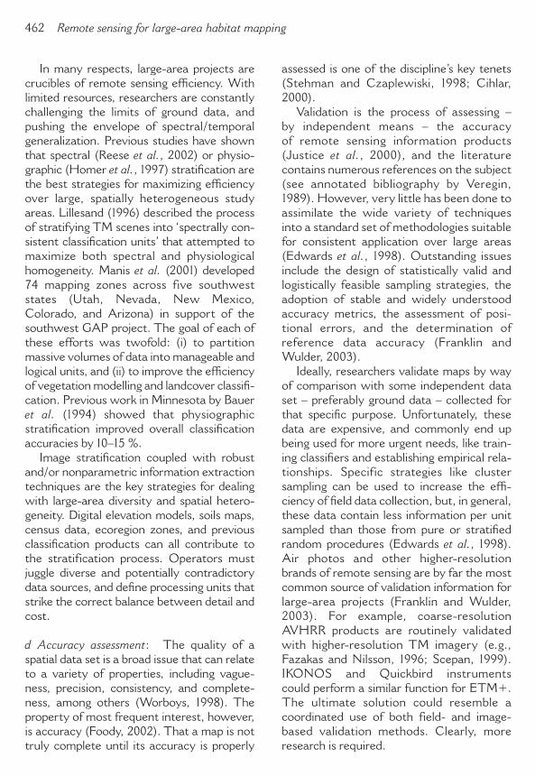
d Accuracy assessment: The quality of aspatial data set is a broad issue that can relateto a variety of properties, including vague-ness, precision, consistency, and complete-ness, among others (Worboys, 1998). Theproperty of most frequent interest, however,is accuracy (Foody, 2002). That a map is nottruly complete until its accuracy is properly

assessed is one of the discipline’s key tenets(Stehman and Czaplewiski, 1998; Cihlar,2000).

Validation is the process of assessing –by independent means – the accuracyof remote sensing information products(Justice et al., 2000), and the literaturecontains numerous references on the subject(see annotated bibliography by Veregin,1989). However, very little has been done toassimilate the wide variety of techniquesinto a standard set of methodologies suitablefor consistent application over large areas(Edwards et al., 1998). Outstanding issuesinclude the design of statistically valid andlogistically feasible sampling strategies, theadoption of stable and widely understoodaccuracy metrics, the assessment of posi-tional errors, and the determination ofreference data accuracy (Franklin andWulder, 2003).

Ideally, researchers validate maps by wayof comparison with some independent dataset – preferably ground data – collected forthat specific purpose. Unfortunately, thesedata are expensive, and commonly end upbeing used for more urgent needs, like train-ing classifiers and establishing empirical rela-tionships. Specific strategies like clustersampling can be used to increase the effi-ciency of field data collection, but, in general,these data contain less information per unitsampled than those from pure or stratifiedrandom procedures (Edwards et al., 1998).Air photos and other higher-resolutionbrands of remote sensing are by far the mostcommon source of validation information forlarge-area projects (Franklin and Wulder,2003). For example, coarse-resolutionAVHRR products are routinely validatedwith higher-resolution TM imagery (e.g.,Fazakas and Nilsson, 1996; Scepan, 1999).IKONOS and Quickbird instrumentscould perform a similar function for ETM�.The ultimate solution could resemble acoordinated use of both field- and image-based validation methods. Clearly, moreresearch is required.


V Linking information needswith remote sensing strategyEcosystems are a somewhat abstract con-cept, and there are competing viewpoints asto which elements are important to map forthe purpose of science and management overlarge areas. Graetz (1990) suggested that thecharacteristics of ecosystems are determinedby the primary trophic level – the vegetation –and that vegetation can therefore be taken asthe functional equivalent of terrestrial eco-systems. Remote sensing scientists havebeen quick to adopt this viewpoint, sincevegetative units are much simpler to mapthan the complex interplay of physical (soils,climate, topography) and biological (wildlife,vegetation, micro-organisms) agents thatdefine the alternative viewpoint.

Unfortunately, many remote sensingproducts can be criticized for presenting anoverly simplistic representation of vegetation,perhaps contributed to by historical limita-tions of satellite data and the ubiquitous useof classification as an information extractiontechnique. However, both of these factorshave undergone recent change, with thegrowing number and availability of commer-cial and noncommercial satellites acquiringdata with ever-increasing spatial, spectral,and temporal dimensions (Phinn, 1998).While these newfound choices have thepotential to greatly enhance our ability toconduct ecological monitoring and manage-ment, they also present unique challengessurrounding the selection of appropriate dataand techniques. The discussion of infomation-extraction strategies for use in large-areaecosystem management applications musttherefore begin with a review of the remotesensing scene model, and how it relates tovegetation as a hierarchical, multiscalephenomenon.

1 Multiscale vegetation structureUnderstanding the structure of complex,natural systems is a key challenge for alldisciplines dealing with these phenomena(Marceau and Hay, 1999). Contemporary

works in landscape ecology (e.g., Gardneret al., 2001; Turner et al., 2001) emphasizethe interaction between vegetation standsdistributed across the Earth’s surface.This ‘mosaic of patches’ implies a certainconceptual model concerning the nature ofvegetation, which can be articulated formallyas complex systems theory. Complex systemstheory describes the behaviour of ecologicalsystems characterized by a large number ofcomponents interacting in a nonlinear wayand exhibiting adaptive properties throughtime (Kay, 1991; Hay et al., 2002). An impor-tant characteristic of complex systems is thatthey intuitively take the form of a nestedhierarchy, in that finer categorical divisions(leaf, canopy) are nested within broader ones(tree, stand). This hierarchical structure isemployed by many classification systems intheir attempt to organize vegetation byprocess rate, scale, or taxonomy (seesummaries by J. Franklin and Woodcock,1997, and S.E. Franklin, 2001).

Woodcock and Harward (1992) presenteda hierarchical model that describes patterns ofmatter and energy flux in a forested scenethat consists (in ascending order) oftrees/gaps, stands, forest types, and scenes.Their model compares closely to Urbanet al.’s (1987) process-based organization ofvegetation into gaps, stands, cover type,provinces, and biomes. The stand (oftenreferred to as a ‘patch’ in the landscapeecology literature) is defined as a contiguousarea of similar species composition, plantcover, and plant size distribution (J. Franklinand Woodcock, 1997). Trees and gaps arenested within stands, which in turn aresubsumed by larger landscape units or covertypes, defined by Cousins (1993) as a complexof systems that form a recognizable entity.While there is some discussion regarding thescale of cover type units (e.g., Forman andGodron, 1986; Urban et al., 1987; Turneret al., 2001) they are generally considered tobe on the order of 1000s of hectares, andcorrespond quite closely to the Level IIclasses of Anderson et al. (1976).


While differences between the variousclassification systems in use (spatial,taxonomic, process-based) can create consid-erable confusion, the understanding of vege-tation as a complex system – and subsequentadoption of one or more hierarchies – isimportant to large-area habitat mappingprojects for the following reasons:1. they represent the foundation of commu-

nication between resource managers andremote sensing specialists;

2. they provide a framework for conductingmultiscale mapping and modelling activities;

3. they provide a conceptual basis for linkingecological information to the remotesensing scene model and subsequentinformation extraction techniques.

2 The scene modelStrahler et al. (1986) described the remotesensing model as having three distinct compo-nents: the sensor, the atmosphere, and thescene. The scene model comprises the area ofinterest, which, in a forest, is composed of aforested portion of the Earth’s surface viewedat a specific scale. For many applications, it isappropriate to consider the scene as a spatialarrangement of discrete two- or three-dimensional objects distributed on a back-ground (Jupp et al., 1988; 1989). In realscenes, objects are formed by spectrallyhomogeneous pixels, and can take manydifferent forms depending on scale. For exam-ple, a conifer forest scene could be modelledat a detailed scale as a series of two-dimensional objects composed of sunlit andshaded patches of forest and understory, or,at a broader scale, as a mosaic of structurallyhomogenous forest stands.

The relationship between the size of theobjects and the spatial resolution of the scenefollows one of two types: H-resolution orL-resolution (Strahler et al., 1986). TheH-resolution case occurs when the pixelsize of the scene is significantly smallerthan the objects of investigation, while the L-resolution case occurs when pixelsare larger than objects (Figure 2). This

designation is important, since it describesthe fundamental relationship between theobjects of interest and the spatial resolution ofthe image, which in turn governs thechoice of subsequent information extractiontechniques.

Generally speaking, H-resolution imagesare best suited for classification, since theobjects of interest occur over areas largerthan individual pixels. Depending on the spe-cific structure of the scene, analysts canemploy a wide variety of image processingtechniques to extract the variables necessaryfor consistent discrimination, and may employresampling (Franklin and McDermid, 1993) orsegmentation (Woodcock and Harward,1992) strategies to better define the objects ofinvestigation. L-resolution scenes, on theother hand, are more suited to per-pixelroutines such as vegetation indices(Satterwhite, 1984; Cohen, 1991), empirical(Moisen and Edwards, 1999; Cohen et al.,2002) or physical (Goel, 1988; Scarth andPhinn, 2000) models, and spectral mixtureanalysis routines (Peddle et al., 1999) thatrelate sub-pixel biophysical properties tomultispectral reflectance measurements.

A critical characteristic of remote sensingscenes is the following: since natural systemsare composed of objects in a multiscalehierarchy, a single image can be both H-resolution with respect to some types ofinformation and L-resolution with respect toothers. Following Woodcock and Harward’s(1992) hierarchical forest scene modeldescribed earlier, a Landsat ETM� imagewould be L-resolution at the tree/gap level,since each 30 m pixel consumes severaltree/gap objects (top part of Figure 2).However, the same 30 m imagery would beconsidered H-resolution with respect tostands, which may cover 10s or 100s of hectaresand consume many individual pixels (bottompart of Figure 2). As a result, the ‘correct’ infor-mation extraction strategy for ecosystem man-agement can vary greatly, and depends jointlyon (i) the scale of information desired, and (ii)the spatial resolution of the image used.


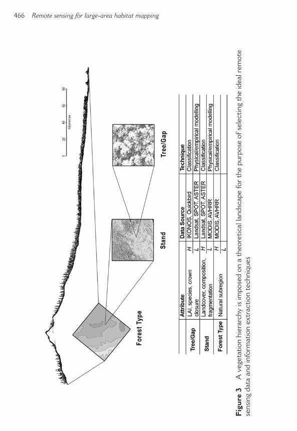
3 A framework for applicationPhinn et al. (2003) presented a framework forselecting the appropriate remote sensing datafor environmental scientists. The processconsists of the following six steps: (i) identifythe information requirements for the project;(ii) organize the information needs in terms ofan ecological hierarchy; (iii) conduct anexploratory analysis using existing digitaldata; (iv) identify the ideal remote sensingdata, considering spatial, spectral, radiometric,

and temporal dimensions; (v) select and applya suitable set of information extractiontechniques; and (vi) conduct a cost benefitanalysis. This process can be visualized withthe help of Figure 3: a hypothetical landscapethat is to be the study area of a regionalhabitat-mapping project. By identifyingvarious vegetation attributes as the requiredinformation products, we can adopt a multiscale hierarchy that organizes the scene inascending scale as tree/gap, stand, and


Figure 2 H- and L-resolution scene models for a forested scene. At the tree/gaplevel (top), Landsat ETM � multispectral pixels are L-resolution, while IKONOSpanchromatic pixels are H-resolution. At the stand level (bottom) LandsatETM � multispectral pixels are H-resolution, while MODIS band 3 pixels areL-resolution


Fig

ure

3A

veg

etat

ion

hier

arch

y is

impo

sed

on a

the

oret

ical

land

scap

e fo

r th

e pu

rpos

e of

sel

ectin

g th

e id

eal r

emot

ese

nsin

g da

ta a

nd in

form

atio

n ex

trac

tion

tech

niqu

es

cover type. Specifications for the idealremote sensing data can vary, depending onvegetation conditions, study area size, andavailable image processing techniques. Figure 3 offers H- and L- resolutionsuggestions at each level of the hierarchy.The choice of data should dictate – at leastinitially – the subsequent image processingtechniques pursued: generally, classificationfor H-resolution data and physical or empiricalmodelling for L-resolution cases. Assessingthe benefits of the resulting investmentshould take into account, among otherthings, the accuracy of the informationproducts generated, the value of the resultinghabitat maps, and the utility of the vegetationdatabase for other resource managementapplications.

VI Summary and conclusionsA strong alliance is forming between remotesensing and ecology to address the challengeof large-area habitat mapping. However, theharmony of this multidisciplinary approach toscience is hindered by miscommunicationand the lack of common understanding.Pioneering work has demonstrated thepromise of geospatial tools in crossdiscipli-nary work, but a tremendous amount ofresearch yet remains. Image classification,per-pixel models, and spatial pattern analysistechniques are effective tools for extractinginformation, but scientists and resourcemanagers require guidance for their effectiveapplication. A framework that combineshierarchy theory with elements of the remotescene model presents a mechanism for linkinginformation needs with image processingtechnique, as well as a foundation for com-munication between ecologists and specialistsin remote sensing. Future research shouldexplore the integrated role of new remotesensing instruments and emerging technolo-gies, develop techniques for constructingmultiscale vegetation databases over largeareas, and test the utility of these databasesfor supporting diverse environmentalapplications.

ReferencesAllen, T.F.H. and Hoekstra, T.W. 1992: Toward a

unified ecology. NewYork: Columbia University Press.Allen, T.R. 2000: Topographic normalization of

Landsat Thematic Mapper data in three mountainenvironments. Geocarto International 15, 13–19.

Anderson, J.R., Hardy, E.E., Roach, J.T. andWitmer, R.E. 1976: A land use and land coverclassification system for use with remote sensor data.US Geological Survey Professional Paper 964,Washington, DC.

Asner, G.P., Treuharft, R.N. and Law, B.E. 2000:Vegetation structure from quantitative fusion of hyper-spectral optical and radar interferometric remotesensing. AVIRIS Proceedings: 2000. Retrieved 29April 2005 from ftp://popo.jpl.nasa.gov/pub/docs/workshops/00_docs/toc.html

Atkinson, P.M. and Tatnall, A.R.L. 1997: Neuralnetworks in remote sensing. International Journal ofRemote Sensing 18, 699–709.

Barandela, R. and Juarez, M. 2002: Supervisedclassification of remotely sensed data with ongoinglearning capability. International Journal of RemoteSensing 23, 4965–70.

Bauer, M.E., Burk, T.E., Ek, A.R., Coppin, P.R.,Lime, S.D., Walsh, T.A., Walters, D.K., Befort, W. and Heinzen, D.F. 1994: Satellite inven-tory of Minnesota forest resources. PhotogrammetricEngineering and Remote Sensing 63, 59–67.

Begon, M., Harper, J.L. and Townsend, C.R. 1990:Ecology: individuals, populations and communities(second edition). Boston, MA: Blackwell.

Binaghi, E., Madella, P., Grazia Montesano, M. andRampini, A. 1997: Fuzzy contextual classification ofmultisource remote sensing images. IEEE Transactionson Geoscience and Remote Sensing 28, 540–51.

Bolstad, P.V. and Gower, S.T. 1992: Improved classifi-cation of forest vegetation in northern Wisconsinthrough a rule-based combination of soils, terrain, andLandsat Thematic Mapper data. Forest Science 38,5–20.

Bolstad, P.V. and Lillesand, T.M. 1992: Flexibleintegration of satellite imagery and thematic spatialdata. Photogrammetric Engineering and RemoteSensing 58, 965–71.

Borak, J.S. and Strahler, A.H. 1999: Feature selectionand land cover classification of a MODIS-like data setfor a semiarid environment. International Journal ofRemote Sensing 20, 919–38.

Brodley, C. and Friedl, M. 1999: Identifying mislabeledtraining data. Journal of Artificial Intelligence Research11, 131–67.

Brown de Colstoun, E.C., Story, M.H., Thompson,C., Commisso, K., Smith, T.G. and Irons, J.R.2003: National park vegetation mapping using multi-temporal Landsat 7 data and a decision tree classifier.Remote Sensing of Environment 85, 316–27.


Carroll, C., Zielinski, W.J. and Noss, R.F. 1999:Using presence-absence data to build and test spatialhabitat models for the fisher in the Klamath region,USA. Conservation Biology 13, 1344–59.

Chavez, P.S. Jr 1988: An improved dark-object subtrac-tion technique for atmospheric scattering correctionof multispectral data. Remote Sensing of Environment24, 459–79.

Ciarniello, L.M., Boyce, M.S. and Beyer, H. 2002:Grizzly bear habitat selection along the Parsnip River,British Columbia. A report prepared for the BritishColumbia Ministry of Forests, Prince George ForestRegion, 24 pp. Retrieved 29 April 2000 fromweb.unbc.ca/parsnip-grizzly/progress/RSF_Grizzly.pdf

Cihlar, J. 2000: Land cover mapping of large areas fromsatellites: status and research priorities. InternationalJournal of Remote Sensing 2, 1093–14.

Cihlar, J., Chen, J., Li, Z., Fedosejevs, G.,Adair, M., Park, W., Fraser, R., Trishchenko, A.,Guindon, B. and Stanley, D. 2002: GeoComp-n,an advanced system for the processing of coarse andmedium resolution satellite data. Part 2: biophysicalproducts for the northern ecosystem. CanadianJournal of Remote Sensing 28, 21–44.

Civco, D.L. 1989: Topographic normalization of LandsatThematic Mapper digital imagery. PhotogrammetricEngineering and Remote Sensing 55, 1303–309.

Clausi, D.A. 2002: An analysis of co-occurrence tex-ture statistics as a function of grey level quantization.Canadian Journal of Remote Sensing 28, 45–62.

Cohen, W.B. 1991: Response of vegetation indices tochanges in three measures of leaf water stress.Photogrammetric Engineering and Remote Sensing 57,195–202.

Cohen, W.B. and Spies, T.A. 1992: Estimating struc-tural attributes of douglas-fir/western hemlock foreststands from Landsat and SPOT imagery. RemoteSensing of Environment 41, 1–17.

Cohen, W.B., Maiersperger, T.K., Gower, S.T. andTurner, D.P. 2003: An improved strategy for regres-sion of biophysical variables and Landsat ETM � data.Remote Sensing of Environment 84, 561–71.

Cohen, W.B., Maiersperger, T.K., Spies, T.A. andOtter, D.R. 2001: Modelling forest cover attributesas continuous variables in a regional context withThematic Mapper data. International Journal ofRemote Sensing 22, 2279–310.

Cohen, W.B., Spies, T.A., Alig, R.J., Oetter, D.R.,Maiersperger, T.K. and Fiorella, M. 2002:Characterizing 23 years (1972–1995) of standreplacement disturbance in western Oregon forestswith Landsat imagery. Ecosystems 5, 122–37.

Cohen, W.B., Spies, T.A. and Fiorella, M. 1995:Estimating the age and structure of forests in amulti-ownership landscape of western Oregon,U.S.A. International Journal of Remote Sensing 16,721–46.

Colinvaux, P.A. 1986: Ecology. New York: Wiley.Collin, P.H. 1988: Dictionary of ecology and the environ-

ment. London: Peter Collin Publishing.Conese, C., Gilabert, M.A., Maselli, F. and Bottai, L.

1993: Topographic normalization of TM scenesthrough the use of an atmospheric correction method and digital terrain models. PhotogrammetricEngineering and Remote Sensing 59, 1745–53.

Corsi, F., de Leeuw, J. and Skidmore, A. 2000:Modeling species distribution with GIS. In Boitani, L.and Fuller, T.K., editors, Research techniques in animalecology: controversies and consequences, New York:Columbia University Press, 389–434.

Corsi, F., Dupre, E. and Boitani, J. 1999: Large-scalemodel of wolf distribution in Italy for conservationplanning. Conservation Biology 13, 150–59.

Cousins, S.H. 1993: Hierarchy in ecology: its relevance tolandscape ecology and geographic information systems.In Haines-Young, R., Green, D.R. and Cousins, S.,editors, Landscape ecology and geographic informationsystems, New York: Taylor and Francis, 75–86.

Crist, E.P. and Cicone, R.C. 1984: A physically-basedtransformation of Thematic Mapper data – the TMtasseled cap. IEEE Transactions on Geoscience andRemote Sensing GE-22, 256–63.

Culvenor, D.S. 2003: Extracting individual treeinformation: a survey of techniques for high spatialresolution imagery. In Wulder, M.A. and Franklin, S.E.,editors, Remote sensing of forest environments: conceptsand case studies, Boston, MA: Kluwer AcademicPublishers, 255–78.

Danks, F.S. and Klein, D.R. 2002: Using GIS to predictpotential wildlife habitat: a case study of muxoxen innorthern Alaska. International Journal of RemoteSensing 23, 4611–32.

Dechka, J.A., Peddle, D.R., Franklin, S.E. andStenhouse, G.B. 2000: Grizzly bear habitatmapping using evidential reasoning and maximumlikelihood classifiers: a comparison. Proceedings, 22ndCanadian Symposium on Remote Sensing, Victoria,BC, 393–402.

DeFries, R.S. and Belward, A.S. 2000: Global andregional land cover characterization from satellitedata: and introduction to the special issue. Inter-national Journal of Remote Sensing 21, 1083–92.

DiGregio, A. and Jansen, L.J.M. 2000: Land CoverClassification System (LCCS): classification conceptsand user manual. Rome: Food and AgricultureOrganization of the United Nation. Retrieved 29April 2005 from www.africover.org/download/manuals/LCCSMS20.pdf

Edwards, T.C., Moisen, G.G. and Cutler, D.R. 1998:Assessing map accuracy in a remotely sensed,ecoregion-scale cover map. Remote Sensing ofEnvironment 63, 73–83.

Edwards, T.C., Moisen, G.G., Frescino, T.S. andLawler, J.J. 2002: Use of forest inventory analysis


information in wildlife habitat modelling: a process forlinking multiple scales. Proceedings of the FIAScience Symposium, Traverse City, MI.

Elkie, P.C., Rempel, S. and Carr, A.P. 1999: Patchanalysts user’s manual: a tool for quantifying landscapestructure. Ontario Ministry of Natural ResourcesNWST Technical Manual TM-001. Thunder Bay,Ontario: Queen’s Printer for Canada. Retrieved 29April 2005 from http://sevilleta.unm.edu/techno-logy/reference/esri/patch_habitat/nwtm002.pdf

Eve, M.D. and Merchant, J.W. 1998: A nationalsurvey of land cover mapping protocols used in thegap analysis program. Retrieved 29 April 2005 from theCenter for Advanced Land Management InformationTechnologies at www.calmit.unl.edu/gapmap

Fayyad, U.M. and Irani, K.B. 1992: On the handling ofcontinuous-valued attributes in decision tree genera-tion. Machine Learning 8, 87–102.

Fazakas, Z. and Nilsson, M. 1996: Volume and forestcover over southern Sweden using AVHRR datacalibrated with TM data. International Journal ofRemote Sensing 17, 1701–709.

Fleming, M.D. and Hoffer, R.M. 1975: Computer-aided analysis of landsat-1 MSS data: a comparison ofthree approaches, including a ‘modified clustering’approach. Laboratory for Application of RemoteSensing Informations Note 072475. West Lafayette,IN: Purdue University.

Foody, G.M. 1996a: Approaches for the production andevaluation of fuzzy land cover classifications fromremotely sensed data. International Journal of RemoteSensing 17, 1317–40.

— 1996b: Fuzzy modelling of vegetation fromremotely sensed imagery. Ecological Modelling 85,Pages 3–12.

— 1999: The continuum of classification fuzziness inthematic mapping. Photogrammetric Engineering andRemote Sensing 65, 443–51.

— 2002: State of land cover classification accuracy assess-ment. Remote Sensing of Environment 80, 185–201.

Forman, R.T.T. and Godron, M. 1986: Landscapeecology. New York: Wiley.

Franklin, J. 1995: Predictive vegetation mapping:geographic modeling of biospatial patterns in relationto environmental gradients. Progress in PhysicalGeography 19, 474–99.

Franklin, J. and Stephenson, J. 1996: Integrating GISand remote sensing to produce regional vegetationdatabases: attributes related to environmental model-ing. Retrieved 29 April 2005 from www.sbg.ac.at/geo/idrisi/gis_environmental_modeling/sf_papers/franklin_janet/my_paper.html

Franklin, J. and Woodcock, C.E. 1997: Multiscalevegetation data for the mountains of southernCalifornia. In Quattrochi, D.A. and Goodchild, M.F.,editors, Scale in remote sensing and GIS, New York:Lewis Publishers, 141–68.

Franklin, J., Phinn, S.R., Woodcock, C.E. andRogan, J. 2003: Rationale and conceptual frame-work for classification approaches to assess forestresources and properties. In Wulder, M.A. andFranklin, S.E., editors, Remote sensing of forestenvironments: concepts and case studies, Boston, MA:Kluwer Academic Publishers, 279–300.

Franklin, S.E. 1991: Image transformations in moun-tainous terrain and the relationship to surfacepatterns. Computers and Geoscience 17, 1137–49.

— 2001: Remote sensing for sustainable forest manage-ment. New York: Lewis Publishers.

Franklin, S.E. and McDermid, G.J. 1993: Empiricalrelations between digital SPOT HRV and CASIimagery and lodgepole pine (Pinus contorta) foreststand parameters. International Journal of RemoteSensing 14, 2331–48.

Franklin, S.E. and Moulton, J.E. 1990: Variability andclassification of Landsat Thematic Mapper spectralresponse in southwest Yukon. Canadian Journal ofRemote Sensing 16, 2–13.

Franklin, S.E. and Wulder, M.A. 2003: Remote sens-ing methods in high spatial resolution satellite dataland cover classification of large area. Progress inPhysical Geography 26, 173–205.

Franklin, S.E., Hall, R.J., Smith, L. and Gerylo, G.R.2003: Discrimination of conifer height, age, andcrown closure classes using Landsat-5 TM imagery inthe Canadian Northwest Territories. InternationalJournal of Remote Sensing 24, 1823–34.

Franklin, S.E., Stenhouse, G.B., Hansen, M.J.,Popplewell, C.C., Dechka, J.A. and Peddle, D.R.2001: An integrated decision tree approach (IDTA) tomapping landcover using satellite remote sensing insupport of grizzly bear habitat analysis in the Albertayellowhead ecosystem. Canadian Journal of RemoteSensing 27, 579–92.

Frescino, T.S., Edwards, T.C. and Moisen, G.G.2001: Modeling spatially explicit forest structuralattributes using generalized additive models. Journalof Vegetation Science 12, 15–26.

Friedl, M.A. and Brodley, C.E. 1997: Decision treeclassification of land cover from remotely senseddata. Remote Sensing of Environment 61, 399–409.

Fung, T. and LeDrew, E.F. 1987: Application ofprincipal components analysis to change detection.Photogrammetric Engineering and Remote Sensing 53,1649–58.

García Borboroglu, P., Yorio, P., Boersma, P.D.,del Valle, H. and Bertellotti, M. 2002: Habitat useand breeding distribution of Magellanic penguins innorthern San Jorge Gulf, Patagonia, Argentina. Auk119, 233–39.

Gardner, R.H., Kemp, W.M., Kennedy, V.S. andPetersen, J.E., editors 2001: Scaling relations inexperimental ecology. New York: Columbia UniversityPress.


Goel, N.S. 1988: Models of vegetation canopy reflectanceand their use in estimation of biophysical parametersfrom reflectance data. New York: Gordon and BreachPublishing Group (now Taylor and Francis), 222 pp.

Gould, W.A., Edlund, S., Zoltai, S., Raynolds, M.,Walker, D.A. and Maier, H. 2002: Canadian arcticvegetation mapping. International Journal of RemoteSensing 23, 4597–609.

Graetz, R.D. 1990: Remote sensing of terrestrialecosystem structure: an ecologist’s pragmatic view.In Hobbs, R.J. and Mooney, H.A., editors, Remotesensing of biosphere functioning, New York: Springer,5–30.

Gu, D. and Gillespie, A. 1998: Topographic normaliza-tion of Landsat TM images of forest based on sub-pixel sun-canopy-sensor geometry. Remote Sensing ofEnvironment 64, 166–75.

Gustafsen, E.J. 1998: Quantifying landscape spatialpattern: what is the state of the art? Ecosystems 1,143–56.

Haines-Young, R. and Chopping, M. 1996:Quantifying landscape structure: a review of land-scape indices and their application to forested land-scapes. Progress in Physical Geography 20, 418–45.

Hall, F.G., Strebel, D.E., Nickeson, J.E. and Goetz, S.J. 1991: Radiometric rectification: toward acommon radiometric response among multidate,multisensor images. Remote Sensing of Environment35, 11–27.

Hall, L.S., Krausman, P.R. and Morrison, M.L.1997: The habitat concept and a plea for standardterminology. Wildlife Society Bulletin 25, 173–82.

Hansen, M., DeFries, R., Townshend, J.R.G. andSohlberg, R. 2000: Global land cover classificationat 1km resolution using a decision tree classifier.International Journal of Remote Sensing 21, 1331–65.

Hansen, M., Dubayah, R. and DeFries, R. 1996:Classification trees: an alternative to traditional landcover classifiers. International Journal of RemoteSensing 17, 1057–81.

Hansen, M.J., Franklin, S.E., Woudsma, C. andPeterson, M. 2001: Caribou habitat classification andfragmentation analysis of old growth cedar/hemlockforests in British Columbia using Landsat TM and GISdata. Remote Sensing of Environment 77, 50–65.

Haralick, R.M., Shanmugan, K. and Dinstein, I.1973: Textural features for image classification. IEEETransactions on Systems, Man and Cybernetics 3,610–21.

Hargis, C.D., Bissonette, J.A. and Turner, D.L.1999: The influence of forest fragmentation and land-scape pattern on American martens. Journal ofApplied Ecology 36, 157–72.

Harris, P. and Ventura, S. 1995: The integration of geo-graphic data with remotely sensed imagery to improveclassification in an urban area. PhotogrammetricEngineering and Remote Sensing 61, 993–98.

Hay, G.J., Dube, P. Bouchard, A. and Marceau, D.J.2002: A scale-space primer for exploring and quanti-fying complex landscapes. Ecological Modelling 153,27–49.

Herr, A.M. and Queen, L.P. 1993: Crane habitat eval-uation using GIS and remote sensing. PhotogrammetricEngineering and Remote Sensing 59, 1531–38.

Hines, E.M. and Franklin, J. 1997: A sensitivityanalysis of a map of habitat quality for the CaliforniaSpotted Owl (Strix occidentalis occidentalis) insouthern California. Proceedings, SecondInternational Symposium on Biology andConservation of Owls of the Northern Hemisphere.Retrieved 29 April 2005/from www.ncrs.fs.fed.us/epubs/owl/HINES.pdf

Hoffer, R.M. 1994: Challenges in developing and apply-ing remote sensing to ecosystem management. InSample, V.A., editors, Remote sensing and GIS inecosystem management, Washington, DC: IslandPress, 25–40.

Homer, C., Huang, C., Yang, L. and Wylie, B. 2002:Development of a circa 2000 landcover database for theUnited States. US Geological Survey, US Departmentof the Interior. Retrieved 29 April 2005 from land-cover.usgs.gov/pdf/asprs_final.pdf

Homer, C., Ramsey, R., Edwards, T.C. Jr andFalconer, A. 1997: Landscape cover-type modellingusing a multi-scene Thematic Mapper mosaic.Photogrammetric Engineering and Remote Sensing 63,59–67.

Huang, C., Comer, C. and Yang, L. 2003: Regionalforest land cover characterization using mediumspatial resolution satellite data. In Wulder, M.A. andFranklin, S.E., editors, Remote sensing of forestenvironments: concepts and case studies, Boston, MA:Kluwer Academic Publishers, 389–410.

Huguenin, R.L., Karaska, M.A., van Blaricom, D.and Jensen, J.R. 1997: Subpixel classification of baldcypress and tupelo gum trees in Thematic Mapperimagery. Photogrammetric Engineering and RemoteSensing 63, 717–25.

Hutchinson, C.F. 1982: Techniques for combiningLandsat and ancillary data for digital classificationimprovement. Photogrammetric Engineering andRemote Sensing 48, 123–30.

Irons, J.R. and Peterson, G.W. 1981: Texture trans-forms of remote sensing data. Remote Sensing ofEnvironment 11, 359–70.

James, M.E. and Kalluri, S.N.V. 1994: The PathfinderAVHRR land data set: an improved coarse resolutiondata set for terrestrial monitoring. InternationalJournal of Remote Sensing 15, 3347–63.

Jensen, J.R. 1996: Introductory digital image processing,a remote sensing perspective. Upper Saddle River, NJ:Prentice-Hall.

Jensen, J.R. and Cowen, D.C. 1999: Remote sensingof urban/suburban infrastructure and socio-economic


attributes. Photogrammetric Engineering and RemoteSensing 65, 611–22.

Jones, K.B. 1986: Amphibians and reptiles. InCooperider, A.Y., Boyd, R.J. and Stuart, H.R., editors,Inventory and monitoring of wildlife habitat, Denver,CO: US Bureau of Land Management, 267–90.

Jupp, D.L.B., Strahler, A.H. and Woodcock, C.E.1988: Autocorrelation and regularization in digitalimages: I. Basic theory. IEEE Transactions onGeoscience and Remote Sensing 26, 463–73.

— 1989: Autocorrelation and regularization in digitalimages: II. Simple image models. IEEE Transactions onGeoscience and Remote Sensing 27, 247–58.

Justice, C.O. and Townshend, J., 2002: Special issueon the moderate resolution imaging spectroradiome-ter (MODIS): a new generation of land surface mon-itoring. Remote Sensing of Environment 83, 1–2.

Justice, C.O., Belward, A., Morisette, J., Lewis, P.,Privette, J. and Baret, F. 2000: Developments inthe ‘validation’ of satellite sensor products for thestudy of the land surface. International Journal ofRemote Sensing 21, 3383–90.

Kay, J. 1991: A non-equilibrium thermodynamic frame-work for discussing ecosystem integrity. EnvironmentalManagement 15, 483–95.

Kepner, W.G., Jones, K.B. and Chaloud, D.J. 1995:Mid-Atlantic landscape indicators project plan.EPA/620/R-95/003. Washington, DC: Office ofResearch and Development.

Kerr, R.M. 1986: Habitat mapping. In Cooperrider,A.Y., Raymond, J.B. and Stuart H.R., editors,Inventory and monitoring of wildlife habitat, Denver,CO: US Department of the Interior, Bureau of Lands,49–72.

Kimes, D.S. and Kirchner, J.A. 1981: Modeling theeffects of various radiant transfers in mountainousterrain on sensor response. IEEE Transactions onGeoscience and Remote Sensing 19, 100–108.

Kimes, D.S., Nelson, R.F., Salas, W.A. and Skole, D.L. 1999: Mapping and secondarytropical forest and forest age from SPOT HRVdata. International Journal of Remote Sensing 20,3625–40.

Kobler, A. and Adamic, M. 1999: Brown bears inSlovenia: identifying locations for construction ofwildlife bridges across highways. ICOWET IIIProceedings, Missoula, Montana. Retrieved 29April 2005 from http://www.cd.gou.ca/enjoying-alberta/parks/featured/kananaskis/creilg/Kabler.pdf

Krausman, P.R. 1999: Some basic principles of habitatuse. In Launchbaugh, K.L., Sander, K.D. and Mosley,J.C., editors, Grazing behavior of livestock and wildlife,University of Idaho Forest, Wildlife and RangeExperimental Station bulletin 70, 85–90.

Krebs, C.J. 1985: Ecology: the experimental analysis ofdistribution and abundance (third edition). New York:Harper and Row, 800 pp.

Kuncheva, L.I. and Jain, L.C. 1999: Nearest neighborclassifier: simultaneous editing and feature selection.Pattern Recognition Letters 20, 1149–56.

Kurki, S., Nikula, A., Helle, P. and Linden, H. 1998:Abundance of red fox and pine marten in relation tothe composition of boreal forest landscapes. Journalof Animal Ecology 67, 874–86.

Lauver, C.L., Busby, W.H. and Whistler, J.L. 2002:Testing a GIS model of habitat suitability for a declininggrassland bird. Environmental Management 30, 88–97.

Lawler, J.T. and Edwards, T.C. 2002: Landscapepatterns as habitat predictors: building and testingmodels for cavity-nesting birds in the Uinta Mountainsof Utah, USA. Landscape Ecology 17, 233–45.

Lehmkuhl, J.F. and Raphael, M.G. 1993: Habitatpattern around spotted owl locations on theOlympic Peninsula, Washington. Journal of WildlifeManagement 57, 302–15.

Lillesand, T.M. 1994: Strategies for improving the accu-racy and specifity of large-area, satellite-cased landcover inventories. Proceedings of the Symposium,Mapping and GIS, Athens, GA 30, 23–30.

— 1996: A protocol for satellite-based land cover classi-fication in the upper Midwest. In Scott, J.M., Tear,T.H. and Davis, F.W., editors, Gap analysis: a land-scape approach to biodiversity planning, Bethesda,MD: American Society for Photogrammetry andRemote Sensing, 103–18.

Lim, K., Treitz, P., Wulder, M., St-Onge, B. andFlood, M. 2003: Lidar remote sensing of foreststructure. Progress in Physical Geography 27, 88–106.

Lindeman, R.L. 1942: The trophic-dynamic aspect ofecology. Ecology 23, 399–418.

Loveland, T., Merchant, J., Ohlen, D. and Brown, J.1991: Development of a land-cover characteristicsdatabase for the contimerous United States. Photo-grammetric Engineering and Remote Sensing 57,1453–63.

Lunetta, R.S., Alvarez, R., Edmonds, C.M., Lyon, J.G., Elvidge, C.D., Bonifaz, R. andGarcia, C. 2002: NALC/Mexico land-cover mappingresults: implications for assessing landscape condition.International Journal of Remote Sensing 23, 3129–48.

Luque, S.S., Lathrop, R.G. and Bognar, J.A. 1994:Temporal and spatial changes in an area of the NewJersey Pine Barrens. Landscape Ecology 9, 287–300.

Maiden, M. 1994: The Pathfinder project. InternationalJournal of Remote Sensing 15, 3333–45.

Manis, G., Lowry, J. and Ramsey, R.D. 2001:Preclassification: an ecologically predictive landformmodel. GAP Analysis Bulletin 10, United StatesGeological Survey.

Marceau, D.J. and Hay, G.J. 1999: Remote sensingcontributions to the scale issue. Canadian Journal ofRemote Sensing, 25, 357–66.

Mather, P. 1999: Computer processing of remotely sensedimages: an introduction. New York: Wiley.


Mayhew, S. and Penny, A. 1992: The concise Oxford dic-tionary of geography. Oxford: Oxford University Press.

McClain, B.J. and Porter, W.F. 2000: Using satelliteimagery to assess large-scale habitat characteristics ofthe Adirondack Park. Environmental Management 26,553–61.

McDermid, G.J. and Franklin, S.E. 1995: Remotesensing and geomorphometric discrimination of slopeprocesses. Zeitschrift für Geomorphologie N.F.,Supplement Band 101, 165–85.

McGarigal, K. and Marks, B.J. 1995: FRAGSTATS:Spatial pattern analysis program for quantifying land-scape structure. Corvallis, OR: USDA Forest ServiceGeneral Technical Report PNW-GTR-351.

McGovern, E.A., Holden, N.M., Ward, S.M. andCollins, J.F. 2002: The radiometric normalization ofmultitemporal Thematic Mapper imagery of the mid-lands of Ireland – a case study. International Journal ofRemote Sensing 23, 751–66.

McLaren, B.E. and Mahoney, S.P. 2001: Comparisonof forestry-based remote sensing methodologies toevaluate woodland caribou habitat in non-forestedareas of Newfoundland. Forestry Chronicle 77,866–73.

Merriam-Webster 1998: Webster’s revised unabridgeddictionary. Springfield, MA: C. and G. MerriamCompany. Retrieved 2005 from www.dictionary.com

Meyer, M. and Werth, L. 1990: Sateliite data: manage-ment panacea or potential problem? Journal ofForestry 88, 10–13.

Meyer, P., Itten, K.I., Kellenberger, T., Sandmeier, S.and Sandmeier, R. 1993: Radiometric corrections oftopographically induced effects on Landsat TM datain an alpine environment. ISPRS Journal ofPhotogrammetry and Remote Sensing 48, 17–28.

Mladenoff, D.J. and Host, G.E. 1994: Ecologicalperspective: current and potential applications ofremote sensing and GIS to ecosystem analysis. InSample, V.A., editor, Remote sensing and GIS inecosystem management, Washington, DC: IslandPress, 218–42.

Moisen, G.G. and Edwards, T.C. Jr 1999: Use of gen-eralized linear models and digital data in a forestinventory of northern Utah. Journal of Agricultural,Biological, and Environmental Statistics 4, 372–90.

Moore, W.G. 1967: A dictionary of geography. London:A and C Black.

Morrison, M.L., Marcot, B.G. and Mannan, R.W.1992: Wildlife-habitat relationships: concepts and appli-cations. Madison, WI: University of Wisconsin Press.

Murai, H. and Omatu, S. 1997: Remote sensing imageanalysis using a neural network and knowledge-basedprocessing. International Journal of Remote Sensing 18,811–28.

Mustard, J.F. 1993: Relationships of soil, grass, andbedrock over the Kaweah Serpentine Melangethrough mixture analysis of AVIRIS data. RemoteSensing of Environment 44, 293–308.

Natural Resources Canada 1995: Land cover map ofCanada. Ottawa: Natural Resources Canada,Retrieved 29 April 2005 from www.ccrs.nrcan.gc.ca/ccrs/rd/apps/landcov/map_e.html

Nielsen, S.E., Boyce, M.S., Stenhouse, G.B. andMunro, R.H.M. 2003: Development and testing ofphonologically driven grizzly bear habitat models.Ecoscience 10, 1�10.

Norris, D.R., Theberge, M.T. and Theberge, J.B.2002: Forest composition around wolf dens in east-ern Algonquin Provincial Park, Ontario. CanadianJournal of Zoology 80, 866–72.

Odum, E.P. 1971: Fundamentals of ecology. Philadelphia,PA: W.B. Sanders Co., 574 pp.

Ohmann, J.L. and Gregory, M.J. 2002: Predictivemapping of forest composition and structure withdirect gradient analysis and nearest neighbor imputa-tion in coastal Oregon, U.S.A. Canadian Journal ofForest Research 32, 725–41.

O’Neill, R.V., DeAngelis, D.L., Waide, J.B. andAllen, T.F.H. 1986: A hierarchical concept of ecosys-tems. Princeton, NJ: Princeton University Press.

O’Neill, R.V., Krummel, J.R., Gardner, R.H.,Sugihara, G., Jackson, B., DeAngelis, D.L.,Milne, B.T., Turner, M.G., Zygmunt, B.,Christensen, S.W., Dale, V.H. and Graham, R.L.1998: Indices of landscape pattern. Landscape Ecology1, 153–62.

Osborne, P.E., Alonso, J.C. and Bryant, R.G. 2001:Modelling landscape-scale habitat using GIS andremote sensing: a case study with great bustards.Journal of Applied Ecology 38, 458–71.

Palma, L., Beja, P. and Rodrigues, M. 1999: The useof sighting data to analyze Iberian lynx habitat anddistribution. Journal of Applied Ecology 36, 812–24.

Pax-Lenney, M., Woodcock, C.E., Macomber, S.A.,Gopal, S. and Song, C. 2001: Forest mapping witha generalized classifier and Landsat TM data. RemoteSensing of Environment 77, 241–50.

Peddle, D.R. 1995: Knowledge formulation for super-vised evidential classification. PhotogrammetricEngineering and Remote Sensing 61, 409–17.

Peddle, D.R., Hall, F.G. and LeDrew, E.F. 1999:Spectral mixture analysis and geometric-opticalreflectance modeling of boreal forest biophysicalstructure. Remote Sensing of Environment 67, 288–97.

Pielou, E.C. 1975: Ecological diversity. New York: Wiley.Peterson, D.L., Spanner, M.A., Running, S.W. and

Teuber, K.B. 1987: Relationship of ThematicMapper simulator data to leaf area index of temperateconiferous forests. Remote Sensing of Environment 22,323–41.

Phinn, S.R. 1998: A framework for selecting appropri-ate remotely sensed data dimensions for environmen-tal monitoring and management. International Journalof Remote Sensing 19, 3457–63.

Phinn, S.R., Stow, D.A., Franklin, J., Mertes,L.A.K. and Michaelsen, J. 2003: Remote sensed


data for ecosystem analyses: combining hierarchytheory and scene models. Environmental Management31, 429–41.

Piwowar, J.M. and LeDrew, E.F. 1996: Principalcomponents analysis of arctic ice conditions between1978 and 1987 as observed from the SSMR datarecord. Canadian Journal of Remote Sensing 22,390–403.

Plummer, S.E. 2000: Perspectives on combining eco-logical process models and remotely sensed data.Ecological Modelling 129, 169–86.

Radeloff, V.C., Pidgeon, A.M. and Hostert, P. 1999:Habitat and population modelling of roe deer using aninteractive geographic information system. EcologicalModelling 114, 287–304.

Read, J.M. and Lam, N.S.N. 2002: Spatial methodsfor characterizing land cover and detecting land-cover changes for the tropics. International Journal ofRemote Sensing 23, 2457–74.

Reese, H.M., Lillesand, T.M., Nagel, D.E.,Stewart, J.N., Goldmann, R.A., Simmons,T.E., Chipman, J.W. and Tessar, P.A. 2002:Statewide land cover derived from multisea-sonal Landsat TM data: a retrospective of theWISCLAND project. Remote Sensing of Environment82, 224–37.

Riiters, K.H., O’Neill, R.V., Hunsaker, C.T.,Wickham, J.D., Yankee, D.H., Timmins, S.P.,Jones, K.B. and Jackson, B.L. 1995: A factoranalysis of landscape pattern and structure metrics.Landscape Ecology 10, 23–39.

Ripley, B.D. 1996: Pattern recognition and neuralnetworks. Cambridge: Cambridge University Press.

Rogan, J., Franklin, J. and Roberts, D. 2002: Acomparison of methods for monitoring multitemporalvegetation using Thematic Mapper imagery. RemoteSensing of Environment 80, 143–56.

Roseberry, J.L. 1998: Landscape characteristics andspatial patterns of eastern cottontail abundance inIllinois. Transactions of the Illinois State Academy ofScience 91, 167–78.

Roughgarden, J., Running, S.W. and Matson, P.A.1991: What does remote sensing do for ecology?Ecology 72, 1918–22.

Rushton, S.P., Lurz, P.W.W., Fuller, R. and Garson, P.J. 1997: Modelling the distribution ofthe red and grey squirrel at the landscape scale: acombined GIS and population dynamics approach.Journal of Applied Ecology 34, 1137–54.

Satterwhite, M.B. 1984: Discriminating vegetation andsoils using Landsat MSS and Thematic Mapper bandsand band ratios. Proceedings, American Society ofPhotogrammetry 2, 479–85.

Scarth, P. and Phinn, S. 2000: Determining foreststructural attributes using an inverted geometric-optical model in the mixed eucalypt forests, south-east Queensland, Australia. Remote Sensing ofEnvironment 71, 141–57.

Scepan, J. 1999: Thematic validation of high-resolutionglobal land-cover data sets. PhotogrammetricEngineering and Remote Sensing 65, 1051–60.

Schriever, J.R. and Congalton, R.G. 1995: Evaluatingseasonal variability as an aid to cover type mappingfrom Landsat Thematic Mapper data in the north-east. Photogrammetric Engineering and RemoteSensing 61, 321–27.

Scott, J.M., Davis, F., Csuti, B., Noss, R.,Butterfield, B., Groves, C., Anderson, H.,Caicco, S., D’Erchia, F., Edwards, T., Ulliman, J.and Wright, G. 1993: Gap analysis: a geographicapproach to protection of biological diversity. Journalof Wildlife Management, 57(1) Supplement, WildlifeMonographs 123.

Skidmore, A., editor 2002: Environmental modellingwith GIS and remote sensing. New York: Taylor andFrancis.

Skidmore, A.K. and Gauld, A. 1996: Classification ofkangaroo habitat distribution using three GIS models.International Journal of Geographical InformationSystems 10, 441–54.

Stehman, S.V. and Czaplewski, R.L. 1998: Designand analysis for thematic map accuracy assessment:fundamental principles. Remote Sensing ofEnvironment 64, 331–44.

Strahler, A.H., Woodcock, C.E. and Smith, J.A.1986: On the nature of models in remote sensing.Remote Sensing of Environment 20, 121–39.

Smith, J.L.D., Ahern, S.C. and McDougal, C. 1998:Landscape analysis of tiger distribution andhabitat quality in Nepal. Conservation Biology 12,1338–46.

Stelfox, H.A. and Ironside, G.R. 1982: Land/wildlifeintegration no. 2. Proceedings of a technical workshopto discuss the incorporation of wildlife informationinto ecological land surveys. Ecological LandClassification Series 17, Lands Directorate,Environment Canada.

Tokola, T., Sarkeala, J. and van der Linden, M.2001: Use of topographic correction in Landsat TM-based forest interpretation in Nepal. InternationalJournal of Remote Sensing 22, 551–63.

Townsend, P.A. and Foster, J.R. 2002: Terrainnormalization of AVIRIS and Hyperion imagery inforested landscapes. In Green, R.O. editors,Proceedings of the Eighth JPL Airborne EarthScience Workshop, Pasadena, CA, retrieved 29 April 2005 from ftp://pop.jpl.nasa.gov/pub/docs/workshops/02_docs/toc.html

Treitz, P.M. and Howarth, P.J. 2000: Integrating spec-tral, spatial and terrain variables for forest ecosystemclassification. Photogrammetric Engineering andRemote Sensing 66, 305–17.

Trotter, C. 1991: Remotely-sensed data as an informa-tion source for geographical information systems innatural resource management: a review. InternationalJournal of Remote Sensing 5, 225–39.


Turner, M.G., Gardner, R.H. and O’Neill, R.V.2001: Landscape ecology in theory and practice: patternand process. New York: Springer Verlag.

Urban, D.L., O’Neill, R.V. and Shugart, H.H. Jr1987: Landscape ecology. Bioscience 37, 119–27.

United States Fish and Wildlife Service (USFWS)1980a: Habitats as a basis for environmental assess-ment. Ecological Service Manual 101, US Departmentof Interior, Fish and Wildlife Service, Division ofEcological Services. Washington, DC: GovernmentPrinting Office, 26 pp.

— 1980b: Habitat evaluation procedures (HEP).Ecological Service Manual 102, US Department ofInterior, Fish and Wildlife Service, Division ofEcological Services. Washington, DC: GovernmentPrinting Office, 84 pp.

Veregin, H. 1989: Accuracy of spatial databases: anno-tated bibliography. Technical Paper 89, NationalCenter for Geographic Information Analysis,University of California. Santa Barbara, CA.

Verlinden, A. and Masogo, R. 1997: Satellite remotesensing of habitat suitability for ungulates and ostrichin the Kalahari of Botswana. Journal of AridEnvironments 35, 563–74.

Vermonte, E. and Kaufman, Y.J. 1995: Absolute cali-bration of AVHRR visible and near-infrared channelsusing ocean and cloud views. International Journal ofRemote Sensing 16, 2317–40.

Vinluan, J.N. and de Alban, J.D. 2001: Evaluation ofLandsat ETM � data for coastal habitat assessmentin support of fisheries management. Proceedings, 22ndAsian Conference on Remote Sensing, Singapore.Retrieved 29 April 2005 from www.crisp.nus.edu.sg/~acrs2001/pdf/289vinlu.pdf

Wagner, W., Luckman, A., Vietmeier, J., Tansey, K.,Balzter, H., Schmullius, C., Davidson, M.,Gaveau, G., Gluck, M., Le Toan, T., Quegan, S.,Shvidenko, A., Weismann, A. and Yu, J.J. 2003:Large-scale mapping of boreal forest in Siberia usingERS tandem coherence and JERS backscatter data.Remote Sensing of Environment 85, 125–44.

Walker, D.A., Gould, W.A., Maier, H.A. andRaynolds, M.K. 2002: The circumpolar arcticvegetation map: AVHRR-derived base maps, envi-ronmental controls, and integrated mappingprocedures. International Journal of Remote Sensing23, 4551–70.

Wallin, D.O., Elliot, C.C.H., Shugart, H.H.,Tucker, C.J. and Wilhelmi, F. 1992: Satellite

remote sensing of breeding habitat for an Africanweaver-bird. Landscape Ecology 7, 87–99.

Whittaker, R.H., Levin, S.A. and Root, R.B. 1973:Niche, habitat, and ecotope. American Naturalist 107,321–38.

Wickland, D.E. 1991: Mission to planet Earth: theecological perspective. Ecology 72, 1923–33.

Wiens, J.A. 1989: Spatial scaling in ecology. FunctionalEcology 3, 385–97.

Wolter, P.T., Mladenoff., D.J., Host, G.E. andCrow, T.R. 1995: Improved forest classification inthe northern lakes states using multi-temporalLandsat imagery. Photogrammetric Engineering andRemote Sensing 61, 1129–43.

Woodcock, C.E. and Harward, V.J. 1992: Nested-hierarchical scene models and image segmentation.International Journal of Remote Sensing 13, 3167–87.

Woodcock, C.E., Macomber, S.A., Pax-Lenney, M.and Cohen, W.B. 2001: Monitoring large areas forforest change using Landsat: generalization acrossspace, time and Landsat sensors. Remote Sensing ofEnvironment 78, 194–203.

Woolf, A., Nielsen, C.K., Weber, T. and Gibbs-Kieninger, T.J. 2002: Statewide modelling ofbobcat, Lynx rufus, habitat in Illinois, USA. BiologicalConservation 104, 191–98.

Worboys, M. 1998: Imprecision in finite resolutionspatial data. GeoInformatica 2, 257–79.

Wu, J., Shen, W., Sun, W. and Tueller, P.T. 2002.Empirical patterns of the effects of changing scale onlandscape metrics. Landscape Ecology, 17, 761–82.

Wulder, M.A. 2002: Mapping the land cover of theforested area of Canada with Landsat data.Proceedings of the 2002 International Geoscience andRemote Sensing Symposium, Toronto, Ontario.

Wyatt, B., Billington, C., de Bie, K., de Leeuw, J.,Greatorex-Davies, N. and Luxmoore, R. 1994:Guidelines for land cover and land use description andclassification. Final Report to United NationsEnvironment Program/Food and AgricultureOrganisation/International Trade Centre/Institute ofTerrestrial Ecology/World Conservation MonitoringCentre, Huntingdon.

Yapp, R.H. 1922: The concept of habitat. Journal ofEcology 10, 1–17.

Zonneveld, I.S., editor 1995: Land ecology. Anintroduction to landscape ecology as a base for landevaluation, land management and conservation.Amsterdam: SPB Academic Publishing.


i introduction - university of...

Documents