i-tree ecosystem analysis - yale university

i-TreeEcosystem Analysis

Yale University 2020

Urban Forest Effects and ValuesApril 2020

Summary

Understanding an urban forest's structure, function and value can promote management decisions that will improvehuman health and environmental quality. An assessment of the vegetation structure, function, and value of the YaleUniversity 2020 urban forest was conducted during 2020. Data from 6159 trees located throughout Yale University2020 were analyzed using the i-Tree Eco model developed by the U.S. Forest Service, Northern Research Station.

• Number of trees: 6,159

• Tree Cover: 47.98 acres

• Most common species of trees: Eastern white pine, Norway maple, Northern red oak

• Percentage of trees less than 6" (15.2 cm) diameter: 27.4%

• Pollution Removal: 1.299 tons/year ($27.6 thousand/year)

• Carbon Storage: 3.73 thousand tons ($636 thousand)

• Carbon Sequestration: 56.83 tons ($9.69 thousand/year)

• Oxygen Production: 151.6 tons/year

• Avoided Runoff: 71.33 thousand cubic feet/year ($4.77 thousand/year)

• Building energy savings: N/A – data not collected

• Avoided carbon emissions: N/A – data not collected

• Structural values: $9.39 million

Ton: short ton (U.S.) (2,000 lbs)Monetary values $ are reported in US Dollars throughout the report except where noted.Ecosystem service estimates are reported for trees.

For an overview of i-Tree Eco methodology, see Appendix I. Data collection quality is determined by the local datacollectors, over which i-Tree has no control.

Table of Contents

Summary ....................................................................................................................................................................2I. Tree Characteristics of the Urban Forest .................................................................................................................4II. Urban Forest Cover and Leaf Area ..........................................................................................................................7III. Air Pollution Removal by Urban Trees ...................................................................................................................9IV. Carbon Storage and Sequestration......................................................................................................................11V. Oxygen Production ...............................................................................................................................................13VI. Avoided Runoff ...................................................................................................................................................14VII. Trees and Building Energy Use ...........................................................................................................................15VIII. Structural and Functional Values .......................................................................................................................16IX. Potential Pest Impacts .........................................................................................................................................17Appendix I. i-Tree Eco Model and Field Measurements ...........................................................................................19Appendix II. Relative Tree Effects .............................................................................................................................23Appendix III. Comparison of Urban Forests ..............................................................................................................24Appendix IV. General Recommendations for Air Quality Improvement ...................................................................25Appendix V. Invasive Species of the Urban Forest ....................................................................................................26Appendix VI. Potential Risk of Pests .........................................................................................................................27References ...............................................................................................................................................................32

I. Tree Characteristics of the Urban Forest

The urban forest of Yale University 2020 has 6,159 trees with a tree cover of Eastern white pine. The three mostcommon species are Eastern white pine (6.3 percent), Norway maple (5.9 percent), and Northern red oak (5.7percent).

Urban forests are composed of a mix of native and exotic tree species. Thus, urban forests often have a tree diversitythat is higher than surrounding native landscapes. Increased tree diversity can minimize the overall impact ordestruction by a species-specific insect or disease, but it can also pose a risk to native plants if some of the exoticspecies are invasive plants that can potentially out-compete and displace native species. In Yale University 2020,about 62 percent of the trees are species native to North America, while 48 percent are native to Connecticut.Species exotic to North America make up 38 percent of the population. Most exotic tree species have an origin fromAsia (20 percent of the species).

The plus sign (+) indicates the tree species is native to another continent other than the ones listed in the grouping.

Invasive plant species are often characterized by their vigor, ability to adapt, reproductive capacity, and general lackof natural enemies. These abilities enable them to displace native plants and make them a threat to natural areas. Sixof the 178 tree species in Yale University 2020 are identified as invasive on the state invasive species list (ConnecticutInvasive Plant Working Group 2013). These invasive species comprise 8.6 percent of the tree population though theymay only cause a minimal level of impact. The three most common invasive species are Norway maple (5.9 percent ofpopulation), Black locust (1.9 percent), and Tree of heaven (0.5 percent) (see Appendix V for a complete list ofinvasive species).

II. Urban Forest Cover and Leaf Area

Many tree benefits equate directly to the amount of healthy leaf surface area of the plant. Trees cover about 47.98acres of Yale University 2020 and provide 208.7 acres of leaf area.

In Yale University 2020, the most dominant species in terms of leaf area are Northern red oak, Pin oak, and Norwaymaple. The 10 species with the greatest importance values are listed in Table 1. Importance values (IV) are calculatedas the sum of percent population and percent leaf area. High importance values do not mean that these trees shouldnecessarily be encouraged in the future; rather these species currently dominate the urban forest structure.

Table 1. Most important species in Yale University 2020

Species NamePercent

PopulationPercent

Leaf Area IV

Northern red oak 5.7 11.1 16.8

Norway maple 5.9 7.8 13.7

Eastern white pine 6.3 7.3 13.7

Pin oak 5.0 8.1 13.1

Red maple 4.9 5.1 10.0

Sugar maple 4.4 5.5 9.8

Kousa dogwood 4.6 2.1 6.7

crabapple 4.6 1.6 6.2

Honeylocust 3.8 2.0 5.8

American elm 1.3 3.7 5.0

Common ground cover classes (including cover types beneath trees and shrubs) in Yale University 2020 are notavailable since they are configured not to be collected.

III. Air Pollution Removal by Urban Trees

Poor air quality is a common problem in many urban areas. It can lead to decreased human health, damage tolandscape materials and ecosystem processes, and reduced visibility. The urban forest can help improve air quality byreducing air temperature, directly removing pollutants from the air, and reducing energy consumption in buildings,which consequently reduces air pollutant emissions from the power sources. Trees also emit volatile organiccompounds that can contribute to ozone formation. However, integrative studies have revealed that an increase intree cover leads to reduced ozone formation (Nowak and Dwyer 2000).

Pollution removal1 by trees in Yale University 2020 was estimated using field data and recent available pollution and

weather data available. Pollution removal was greatest for ozone (Figure 7). It is estimated that trees remove 1.299tons of air pollution (ozone (O3), carbon monoxide (CO), nitrogen dioxide (NO2), particulate matter less than 2.5

microns (PM2.5)2, and sulfur dioxide (SO2)) per year with an associated value of $27.6 thousand (see Appendix I for

more details).

1 Particulate matter less than 10 microns is a significant air pollutant. Given that i-Tree Eco analyzes particulate matter less than 2.5 microns (PM2.5) which is a

subset of PM10, PM10 has not been included in this analysis. PM2.5 is generally more relevant in discussions concerning air pollution effects on human health.

2 Trees remove PM2.5 when particulate matter is deposited on leaf surfaces. This deposited PM2.5 can be resuspended to the atmosphere or removed during

rain events and dissolved or transferred to the soil. This combination of events can lead to positive or negative pollution removal and value depending onvarious atmospheric factors (see Appendix I for more details).

In 2020, trees in Yale University 2020 emitted an estimated 1610 pounds of volatile organic compounds (VOCs) (1288pounds of isoprene and 322.4 pounds of monoterpenes). Emissions vary among species based on speciescharacteristics (e.g. some genera such as oaks are high isoprene emitters) and amount of leaf biomass. Sixty percentof the urban forest's VOC emissions were from Northern red oak and Pin oak. These VOCs are precursor chemicals toozone formation.³

General recommendations for improving air quality with trees are given in Appendix VIII.

³ Some economic studies have estimated VOC emission costs. These costs are not included here as there is a tendency to add positive dollar estimates of ozoneremoval effects with negative dollar values of VOC emission effects to determine whether tree effects are positive or negative in relation to ozone. Thiscombining of dollar values to determine tree effects should not be done, rather estimates of VOC effects on ozone formation (e.g., via photochemical models)should be conducted and directly contrasted with ozone removal by trees (i.e., ozone effects should be directly compared, not dollar estimates). In addition, airtemperature reductions by trees have been shown to significantly reduce ozone concentrations (Cardelino and Chameides 1990; Nowak et al 2000), but are notconsidered in this analysis. Photochemical modeling that integrates tree effects on air temperature, pollution removal, VOC emissions, and emissions frompower plants can be used to determine the overall effect of trees on ozone concentrations.

IV. Carbon Storage and Sequestration

Climate change is an issue of global concern. Urban trees can help mitigate climate change by sequesteringatmospheric carbon (from carbon dioxide) in tissue and by altering energy use in buildings, and consequently alteringcarbon dioxide emissions from fossil-fuel based power sources (Abdollahi et al 2000).

Trees reduce the amount of carbon in the atmosphere by sequestering carbon in new growth every year. The amountof carbon annually sequestered is increased with the size and health of the trees. The gross sequestration of YaleUniversity 2020 trees is about 56.83 tons of carbon per year with an associated value of $9.69 thousand. SeeAppendix I for more details on methods.

Carbon storage is another way trees can influence global climate change. As a tree grows, it stores more carbon byholding it in its accumulated tissue. As a tree dies and decays, it releases much of the stored carbon back into theatmosphere. Thus, carbon storage is an indication of the amount of carbon that can be released if trees are allowedto die and decompose. Maintaining healthy trees will keep the carbon stored in trees, but tree maintenance cancontribute to carbon emissions (Nowak et al 2002c). When a tree dies, using the wood in long-term wood products,to heat buildings, or to produce energy will help reduce carbon emissions from wood decomposition or from fossil-fuel or wood-based power plants.

Trees in Yale University 2020 are estimated to store 3730 tons of carbon ($636 thousand). Of the species sampled,Northern red oak stores and sequesters the most carbon (approximately 18.5% of the total carbon stored and 13.8%of all sequestered carbon.)

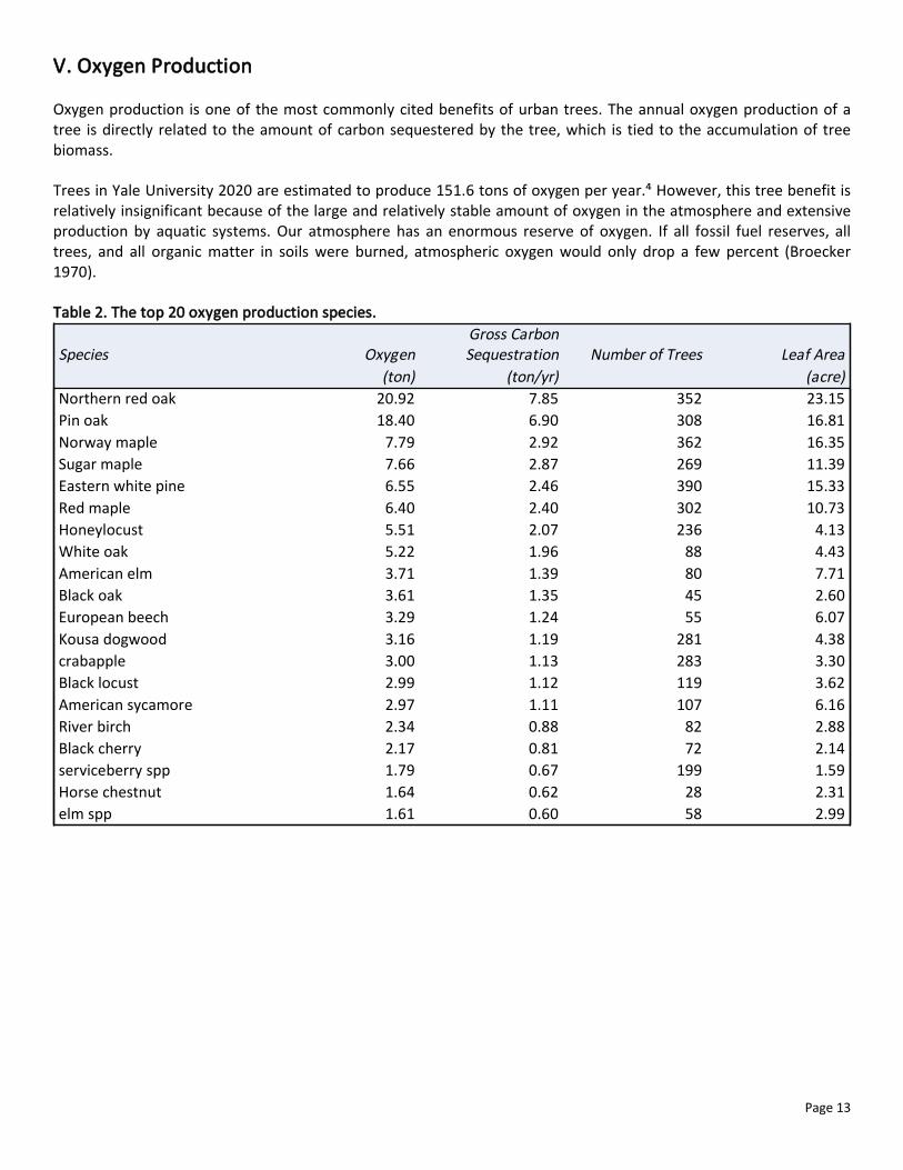
V. Oxygen Production

Oxygen production is one of the most commonly cited benefits of urban trees. The annual oxygen production of atree is directly related to the amount of carbon sequestered by the tree, which is tied to the accumulation of treebiomass.

Trees in Yale University 2020 are estimated to produce 151.6 tons of oxygen per year.⁴ However, this tree benefit isrelatively insignificant because of the large and relatively stable amount of oxygen in the atmosphere and extensiveproduction by aquatic systems. Our atmosphere has an enormous reserve of oxygen. If all fossil fuel reserves, alltrees, and all organic matter in soils were burned, atmospheric oxygen would only drop a few percent (Broecker1970).

Table 2. The top 20 oxygen production species.

Species OxygenGross CarbonSequestration Number of Trees Leaf Area

(ton) (ton/yr) (acre)

Northern red oak 20.92 7.85 352 23.15

Pin oak 18.40 6.90 308 16.81

Norway maple 7.79 2.92 362 16.35

Sugar maple 7.66 2.87 269 11.39

Eastern white pine 6.55 2.46 390 15.33

Red maple 6.40 2.40 302 10.73

Honeylocust 5.51 2.07 236 4.13

White oak 5.22 1.96 88 4.43

American elm 3.71 1.39 80 7.71

Black oak 3.61 1.35 45 2.60

European beech 3.29 1.24 55 6.07

Kousa dogwood 3.16 1.19 281 4.38

crabapple 3.00 1.13 283 3.30

Black locust 2.99 1.12 119 3.62

American sycamore 2.97 1.11 107 6.16

River birch 2.34 0.88 82 2.88

Black cherry 2.17 0.81 72 2.14

serviceberry spp 1.79 0.67 199 1.59

Horse chestnut 1.64 0.62 28 2.31

elm spp 1.61 0.60 58 2.99

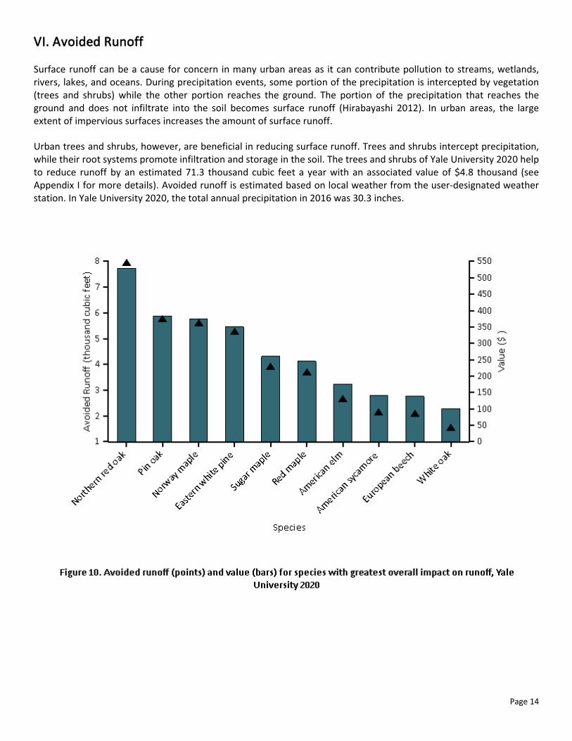
VI. Avoided Runoff

Surface runoff can be a cause for concern in many urban areas as it can contribute pollution to streams, wetlands,rivers, lakes, and oceans. During precipitation events, some portion of the precipitation is intercepted by vegetation(trees and shrubs) while the other portion reaches the ground. The portion of the precipitation that reaches theground and does not infiltrate into the soil becomes surface runoff (Hirabayashi 2012). In urban areas, the largeextent of impervious surfaces increases the amount of surface runoff.

Urban trees and shrubs, however, are beneficial in reducing surface runoff. Trees and shrubs intercept precipitation,while their root systems promote infiltration and storage in the soil. The trees and shrubs of Yale University 2020 helpto reduce runoff by an estimated 71.3 thousand cubic feet a year with an associated value of $4.8 thousand (seeAppendix I for more details). Avoided runoff is estimated based on local weather from the user-designated weatherstation. In Yale University 2020, the total annual precipitation in 2016 was 30.3 inches.

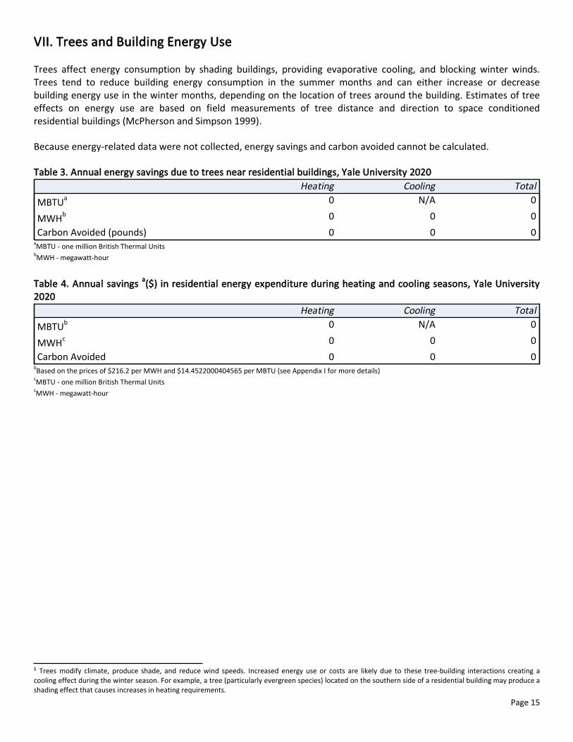
VII. Trees and Building Energy Use

Trees affect energy consumption by shading buildings, providing evaporative cooling, and blocking winter winds.Trees tend to reduce building energy consumption in the summer months and can either increase or decreasebuilding energy use in the winter months, depending on the location of trees around the building. Estimates of treeeffects on energy use are based on field measurements of tree distance and direction to space conditionedresidential buildings (McPherson and Simpson 1999).

Because energy-related data were not collected, energy savings and carbon avoided cannot be calculated.

⁵ Trees modify climate, produce shade, and reduce wind speeds. Increased energy use or costs are likely due to these tree-building interactions creating acooling effect during the winter season. For example, a tree (particularly evergreen species) located on the southern side of a residential building may produce ashading effect that causes increases in heating requirements.

Table 3. Annual energy savings due to trees near residential buildings, Yale University 2020

Heating Cooling Total

MBTUa 0 N/A 0

MWHb 0 0 0

Carbon Avoided (pounds) 0 0 0aMBTU - one million British Thermal Units

bMWH - megawatt-hour

Table 4. Annual savings a($) in residential energy expenditure during heating and cooling seasons, Yale University

2020

Heating Cooling Total

MBTUb 0 N/A 0

MWHc 0 0 0

Carbon Avoided 0 0 0bBased on the prices of $216.2 per MWH and $14.4522000404565 per MBTU (see Appendix I for more details)

cMBTU - one million British Thermal Units

cMWH - megawatt-hour

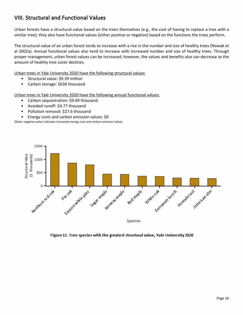
VIII. Structural and Functional Values

Urban forests have a structural value based on the trees themselves (e.g., the cost of having to replace a tree with asimilar tree); they also have functional values (either positive or negative) based on the functions the trees perform.

The structural value of an urban forest tends to increase with a rise in the number and size of healthy trees (Nowak etal 2002a). Annual functional values also tend to increase with increased number and size of healthy trees. Throughproper management, urban forest values can be increased; however, the values and benefits also can decrease as theamount of healthy tree cover declines.

Urban trees in Yale University 2020 have the following structural values:• Structural value: $9.39 million• Carbon storage: $636 thousand

Urban trees in Yale University 2020 have the following annual functional values:• Carbon sequestration: $9.69 thousand• Avoided runoff: $4.77 thousand• Pollution removal: $27.6 thousand• Energy costs and carbon emission values: $0

(Note: negative value indicates increased energy cost and carbon emission value)

IX. Potential Pest Impacts

Various insects and diseases can infest urban forests, potentially killing trees and reducing the health, structural valueand sustainability of the urban forest. As pests tend to have differing tree hosts, the potential damage or risk of eachpest will differ among cities.Thirty-six pests were analyzed for their potential impact and compared with pest rangemaps (Forest Health Technology Enterprise Team 2014) for the conterminous United States to determine theirproximity to New Haven County. Eleven of the thirty-six pests analyzed are located within the county. For a completeanalysis of all pests, see Appendix VII.

Beech bark disease (BBD) (Houston and O’Brien 1983) is an insect-disease complex that primarily impacts Americanbeech. This disease threatens 1.1 percent of the population, which represents a potential loss of $353 thousand instructural value.

Butternut canker (BC) (Ostry et al 1996) is caused by a fungus that infects butternut trees. The disease has sincecaused significant declines in butternut populations in the United States. Potential loss of trees from BC is 0.0 percent($0 in structural value).

The most common hosts of the fungus that cause chestnut blight (CB) (Diller 1965) are American and Europeanchestnut. CB has the potential to affect 0.0 percent of the population ($0 in structural value).

Dogwood anthracnose (DA) (Mielke and Daughtrey) is a disease that affects dogwood species, specifically floweringand Pacific dogwood. This disease threatens 8.7 percent of the population, which represents a potential loss of $261thousand in structural value.

American elm, one of the most important street trees in the twentieth century, has been devastated by the Dutch

elm disease (DED) (Northeastern Area State and Private Forestry 1998). Since first reported in the 1930s, it has killedover 50 percent of the native elm population in the United States. Although some elm species have shown varyingdegrees of resistance, Yale University 2020 could possibly lose 2.5 percent of its trees to this pest ($421 thousand instructural value).

Emerald ash borer (EAB) (Michigan State University 2010) has killed thousands of ash trees in parts of the UnitedStates. EAB has the potential to affect 0.9 percent of the population ($60.4 thousand in structural value).

The gypsy moth (GM) (Northeastern Area State and Private Forestry 2005) is a defoliator that feeds on many speciescausing widespread defoliation and tree death if outbreak conditions last several years. This pest threatens 26.7percent of the population, which represents a potential loss of $3.44 million in structural value.

As one of the most damaging pests to eastern hemlock and Carolina hemlock, hemlock woolly adelgid (HWA) (U.S.Forest Service 2005) has played a large role in hemlock mortality in the United States. HWA has the potential to affect1.4 percent of the population ($133 thousand in structural value).

Quaking aspen is a principal host for the defoliator, large aspen tortrix (LAT) (Ciesla and Kruse 2009). LAT poses athreat to 2.7 percent of the Yale University 2020 urban forest, which represents a potential loss of $169 thousand instructural value.

Although the southern pine beetle (SPB) (Clarke and Nowak 2009) will attack most pine species, its preferred hostsare loblolly, Virginia, pond, spruce, shortleaf, and sand pines. This pest threatens 10.7 percent of the population,which represents a potential loss of $1.12 million in structural value.

Since its introduction to the United States in 1900, white pine blister rust (Eastern U.S.) (WPBR) (Nicholls andAnderson 1977) has had a detrimental effect on white pines, particularly in the Lake States. WPBR has the potentialto affect 6.3 percent of the population ($799 thousand in structural value).

Appendix I. i-Tree Eco Model and Field Measurements

i-Tree Eco is designed to use standardized field data and local hourly air pollution and meteorological data to quantifyurban forest structure and its numerous effects (Nowak and Crane 2000), including:

• Urban forest structure (e.g., species composition, tree health, leaf area, etc.).• Amount of pollution removed hourly by the urban forest, and its associated percent air quality improvement

throughout a year.• Total carbon stored and net carbon annually sequestered by the urban forest.• Effects of trees on building energy use and consequent effects on carbon dioxide emissions from power

sources.• Structural value of the forest, as well as the value for air pollution removal and carbon storage and

sequestration.• Potential impact of infestations by pests, such as Asian longhorned beetle, emerald ash borer, gypsy moth,

and Dutch elm disease.

Typically, all field data are collected during the leaf-on season to properly assess tree canopies. Typical data collection(actual data collection may vary depending upon the user) includes land use, ground and tree cover, individual treeattributes of species, stem diameter, height, crown width, crown canopy missing and dieback, and distance anddirection to residential buildings (Nowak et al 2005; Nowak et al 2008).

During data collection, trees are identified to the most specific taxonomic classification possible. Trees that are notclassified to the species level may be classified by genus (e.g., ash) or species groups (e.g., hardwood). In this report,tree species, genera, or species groups are collectively referred to as tree species.

Tree Characteristics:

Leaf area of trees was assessed using measurements of crown dimensions and percentage of crown canopy missing.In the event that these data variables were not collected, they are estimated by the model.

An analysis of invasive species is not available for studies outside of the United States. For the U.S., invasive speciesare identified using an invasive species list (Connecticut Invasive Plant Working Group 2013)for the state in which theurban forest is located. These lists are not exhaustive and they cover invasive species of varying degrees ofinvasiveness and distribution. In instances where a state did not have an invasive species list, a list was created basedon the lists of the adjacent states. Tree species that are identified as invasive by the state invasive species list arecross-referenced with native range data. This helps eliminate species that are on the state invasive species list, butare native to the study area.

Air Pollution Removal:

Pollution removal is calculated for ozone, sulfur dioxide, nitrogen dioxide, carbon monoxide and particulate matterless than 2.5 microns. Particulate matter less than 10 microns (PM10) is another significant air pollutant. Given that i-Tree Eco analyzes particulate matter less than 2.5 microns (PM2.5) which is a subset of PM10, PM10 has not beenincluded in this analysis. PM2.5 is generally more relevant in discussions concerning air pollution effects on humanhealth.

Air pollution removal estimates are derived from calculated hourly tree-canopy resistances for ozone, and sulfur andnitrogen dioxides based on a hybrid of big-leaf and multi-layer canopy deposition models (Baldocchi 1988; Baldocchiet al 1987). As the removal of carbon monoxide and particulate matter by vegetation is not directly related totranspiration, removal rates (deposition velocities) for these pollutants were based on average measured values fromthe literature (Bidwell and Fraser 1972; Lovett 1994) that were adjusted depending on leaf phenology and leaf area.

Particulate removal incorporated a 50 percent resuspension rate of particles back to the atmosphere (Zinke 1967).Recent updates (2011) to air quality modeling are based on improved leaf area index simulations, weather andpollution processing and interpolation, and updated pollutant monetary values (Hirabayashi et al 2011; Hirabayashiet al 2012; Hirabayashi 2011).

Trees remove PM2.5 when particulate matter is deposited on leaf surfaces (Nowak et al 2013). This deposited PM2.5can be resuspended to the atmosphere or removed during rain events and dissolved or transferred to the soil. Thiscombination of events can lead to positive or negative pollution removal and value depending on variousatmospheric factors. Generally, PM2.5 removal is positive with positive benefits. However, there are some caseswhen net removal is negative or resuspended particles lead to increased pollution concentrations and negativevalues. During some months (e.g., with no rain), trees resuspend more particles than they remove. Resuspension canalso lead to increased overall PM2.5 concentrations if the boundary layer conditions are lower during netresuspension periods than during net removal periods. Since the pollution removal value is based on the change inpollution concentration, it is possible to have situations when trees remove PM2.5 but increase concentrations andthus have negative values during periods of positive overall removal. These events are not common, but can happen.

For reports in the United States, default air pollution removal value is calculated based on local incidence of adversehealth effects and national median externality costs. The number of adverse health effects and associated economicvalue is calculated for ozone, sulfur dioxide, nitrogen dioxide, and particulate matter less than 2.5 microns using datafrom the U.S. Environmental Protection Agency's Environmental Benefits Mapping and Analysis Program (BenMAP)(Nowak et al 2014). The model uses a damage-function approach that is based on the local change in pollutionconcentration and population. National median externality costs were used to calculate the value of carbonmonoxide removal (Murray et al 1994).

For international reports, user-defined local pollution values are used. For international reports that do not have localvalues, estimates are based on either European median externality values (van Essen et al 2011) or BenMAPregression equations (Nowak et al 2014) that incorporate user-defined population estimates. Values are thenconverted to local currency with user-defined exchange rates.

For this analysis, pollution removal value is calculated based on the prices of $1,327 per ton (carbon monoxide),$13,594 per ton (ozone), $1,753 per ton (nitrogen dioxide), $572 per ton (sulfur dioxide), $576,171 per ton(particulate matter less than 2.5 microns).

Carbon Storage and Sequestration:

Carbon storage is the amount of carbon bound up in the above-ground and below-ground parts of woody vegetation.To calculate current carbon storage, biomass for each tree was calculated using equations from the literature andmeasured tree data. Open-grown, maintained trees tend to have less biomass than predicted by forest-derivedbiomass equations (Nowak 1994). To adjust for this difference, biomass results for open-grown urban trees weremultiplied by 0.8. No adjustment was made for trees found in natural stand conditions. Tree dry-weight biomass wasconverted to stored carbon by multiplying by 0.5.

Carbon sequestration is the removal of carbon dioxide from the air by plants. To estimate the gross amount of carbonsequestered annually, average diameter growth from the appropriate genera and diameter class and tree conditionwas added to the existing tree diameter (year x) to estimate tree diameter and carbon storage in year x+1.

Carbon storage and carbon sequestration values are based on estimated or customized local carbon values. Forinternational reports that do not have local values, estimates are based on the carbon value for the United States(U.S. Environmental Protection Agency 2015, Interagency Working Group on Social Cost of Carbon 2015) andconverted to local currency with user-defined exchange rates.

For this analysis, carbon storage and carbon sequestration values are calculated based on $171 per ton.

Oxygen Production:

The amount of oxygen produced is estimated from carbon sequestration based on atomic weights: net O2 release(kg/yr) = net C sequestration (kg/yr) × 32/12. To estimate the net carbon sequestration rate, the amount of carbonsequestered as a result of tree growth is reduced by the amount lost resulting from tree mortality. Thus, net carbonsequestration and net annual oxygen production of the urban forest account for decomposition (Nowak et al 2007).For complete inventory projects, oxygen production is estimated from gross carbon sequestration and does notaccount for decomposition.

Avoided Runoff:

Annual avoided surface runoff is calculated based on rainfall interception by vegetation, specifically the differencebetween annual runoff with and without vegetation. Although tree leaves, branches, and bark may interceptprecipitation and thus mitigate surface runoff, only the precipitation intercepted by leaves is accounted for in thisanalysis.

The value of avoided runoff is based on estimated or user-defined local values. For international reports that do nothave local values, the national average value for the United States is utilized and converted to local currency withuser-defined exchange rates. The U.S. value of avoided runoff is based on the U.S. Forest Service's Community TreeGuide Series (McPherson et al 1999; 2000; 2001; 2002; 2003; 2004; 2006a; 2006b; 2006c; 2007; 2010; Peper et al2009; 2010; Vargas et al 2007a; 2007b; 2008).

For this analysis, avoided runoff value is calculated based on the price of $0.07 per ft³.

Building Energy Use:

If appropriate field data were collected, seasonal effects of trees on residential building energy use were calculatedbased on procedures described in the literature (McPherson and Simpson 1999) using distance and direction of treesfrom residential structures, tree height and tree condition data. To calculate the monetary value of energy savings,local or custom prices per MWH or MBTU are utilized.

For this analysis, energy saving value is calculated based on the prices of $216.20 per MWH and $14.45 per MBTU.

Structural Values:

Structural value is the value of a tree based on the physical resource itself (e.g., the cost of having to replace a treewith a similar tree). Structural values were based on valuation procedures of the Council of Tree and LandscapeAppraisers, which uses tree species, diameter, condition, and location information (Nowak et al 2002a; 2002b).Structural value may not be included for international projects if there is insufficient local data to complete thevaluation procedures.

Potential Pest Impacts:

The complete potential pest risk analysis is not available for studies outside of the United States. The number of treesat risk to the pests analyzed is reported, though the list of pests is based on known insects and disease in the UnitedStates.

For the U.S., potential pest risk is based on pest range maps and the known pest host species that are likely to

experience mortality. Pest range maps for 2012 from the Forest Health Technology Enterprise Team (FHTET) (ForestHealth Technology Enterprise Team 2014) were used to determine the proximity of each pest to the county in whichthe urban forest is located. For the county, it was established whether the insect/disease occurs within the county, iswithin 250 miles of the county edge, is between 250 and 750 miles away, or is greater than 750 miles away. FHTETdid not have pest range maps for Dutch elm disease and chestnut blight. The range of these pests was based onknown occurrence and the host range, respectively (Eastern Forest Environmental Threat Assessment Center; Worrall2007).

Relative Tree Effects:

The relative value of tree benefits reported in Appendix II is calculated to show what carbon storage andsequestration, and air pollutant removal equate to in amounts of municipal carbon emissions, passenger automobileemissions, and house emissions.

Municipal carbon emissions are based on 2010 U.S. per capita carbon emissions (Carbon Dioxide Information AnalysisCenter 2010). Per capita emissions were multiplied by city population to estimate total city carbon emissions.

Light duty vehicle emission rates (g/mi) for CO, NOx, VOCs, PM10, SO2 for 2010 (Bureau of Transportation Statistics2010; Heirigs et al 2004), PM2.5 for 2011-2015 (California Air Resources Board 2013), and CO2 for 2011 (U.S.Environmental Protection Agency 2010) were multiplied by average miles driven per vehicle in 2011 (FederalHighway Administration 2013) to determine average emissions per vehicle.

Household emissions are based on average electricity kWh usage, natural gas Btu usage, fuel oil Btu usage, keroseneBtu usage, LPG Btu usage, and wood Btu usage per household in 2009 (Energy Information Administration 2013;Energy Information Administration 2014)

• CO2, SO2, and NOx power plant emission per KWh are from Leonardo Academy 2011. CO emission per kWhassumes 1/3 of one percent of C emissions is CO based on Energy Information Administration 1994. PM10emission per kWh from Layton 2004.

• CO2, NOx, SO2, and CO emission per Btu for natural gas, propane and butane (average used to represent LPG),Fuel #4 and #6 (average used to represent fuel oil and kerosene) from Leonardo Academy 2011.

• CO2 emissions per Btu of wood from Energy Information Administration 2014.• CO, NOx and SOx emission per Btu based on total emissions and wood burning (tons) from (British Columbia

Ministry 2005; Georgia Forestry Commission 2009).

Appendix II. Relative Tree Effects

The urban forest in Yale University 2020 provides benefits that include carbon storage and sequestration, and airpollutant removal. To estimate the relative value of these benefits, tree benefits were compared to estimates ofaverage municipal carbon emissions, average passenger automobile emissions, and average household emissions.See Appendix I for methodology.

Carbon storage is equivalent to:• Amount of carbon emitted in Yale University 2020 in 2 days• Annual carbon (C) emissions from 2,640 automobiles• Annual C emissions from 1,080 single-family houses

Carbon monoxide removal is equivalent to:• Annual carbon monoxide emissions from 0 automobiles• Annual carbon monoxide emissions from 0 single-family houses

Nitrogen dioxide removal is equivalent to:• Annual nitrogen dioxide emissions from 30 automobiles• Annual nitrogen dioxide emissions from 13 single-family houses

Sulfur dioxide removal is equivalent to:• Annual sulfur dioxide emissions from 161 automobiles• Annual sulfur dioxide emissions from 0 single-family houses

Annual carbon sequestration is equivalent to:• Amount of carbon emitted in Yale University 2020 in 0.0 days• Annual C emissions from 0 automobiles• Annual C emissions from 0 single-family houses

Appendix III. Comparison of Urban Forests

A common question asked is, "How does this city compare to other cities?" Although comparison among cities shouldbe made with caution as there are many attributes of a city that affect urban forest structure and functions, summarydata are provided from other cities analyzed using the i-Tree Eco model.I. City totals for treesCity % Tree Cover Number of Trees Carbon Storage Carbon Sequestration Pollution Removal

(tons) (tons/yr) (tons/yr)

Toronto, ON, Canada 26.6 10,220,000 1,221,000 51,500 2,099

Atlanta, GA 36.7 9,415,000 1,344,000 46,400 1,663

Los Angeles, CA 11.1 5,993,000 1,269,000 77,000 1,975

New York, NY 20.9 5,212,000 1,350,000 42,300 1,676

London, ON, Canada 24.7 4,376,000 396,000 13,700 408

Chicago, IL 17.2 3,585,000 716,000 25,200 888

Phoenix, AZ 9.0 3,166,000 315,000 32,800 563

Baltimore, MD 21.0 2,479,000 570,000 18,400 430

Philadelphia, PA 15.7 2,113,000 530,000 16,100 575

Washington, DC 28.6 1,928,000 525,000 16,200 418

Oakville, ON , Canada 29.1 1,908,000 147,000 6,600 190

Albuquerque, NM 14.3 1,846,000 332,000 10,600 248

Boston, MA 22.3 1,183,000 319,000 10,500 283

Syracuse, NY 26.9 1,088,000 183,000 5,900 109

Woodbridge, NJ 29.5 986,000 160,000 5,600 210

Minneapolis, MN 26.4 979,000 250,000 8,900 305

San Francisco, CA 11.9 668,000 194,000 5,100 141

Morgantown, WV 35.5 658,000 93,000 2,900 72

Moorestown, NJ 28.0 583,000 117,000 3,800 118

Hartford, CT 25.9 568,000 143,000 4,300 58

Jersey City, NJ 11.5 136,000 21,000 890 41

Casper, WY 8.9 123,000 37,000 1,200 37

Freehold, NJ 34.4 48,000 20,000 540 22

II. Totals per acre of land areaCity Number of Trees/ac Carbon Storage Carbon Sequestration Pollution Removal

(tons/ac) (tons/ac/yr) (lb/ac/yr)

Toronto, ON, Canada 64.9 7.8 0.33 26.7

Atlanta, GA 111.6 15.9 0.55 39.4

Los Angeles, CA 19.6 4.2 0.16 13.1

New York, NY 26.4 6.8 0.21 17.0

London, ON, Canada 75.1 6.8 0.24 14.0

Chicago, IL 24.2 4.8 0.17 12.0

Phoenix, AZ 12.9 1.3 0.13 4.6

Baltimore, MD 48.0 11.1 0.36 16.6

Philadelphia, PA 25.1 6.3 0.19 13.6

Washington, DC 49.0 13.3 0.41 21.2

Oakville, ON , Canada 78.1 6.0 0.27 11.0

Albuquerque, NM 21.8 3.9 0.12 5.9

Boston, MA 33.5 9.1 0.30 16.1

Syracuse, NY 67.7 10.3 0.34 13.6

Woodbridge, NJ 66.5 10.8 0.38 28.4

Minneapolis, MN 26.2 6.7 0.24 16.3

San Francisco, CA 22.5 6.6 0.17 9.5

Morgantown, WV 119.2 16.8 0.52 26.0

Moorestown, NJ 62.1 12.4 0.40 25.1

Hartford, CT 50.4 12.7 0.38 10.2

Jersey City, NJ 14.4 2.2 0.09 8.6

Casper, WY 9.1 2.8 0.09 5.5

Freehold, NJ 38.3 16.0 0.44 35.3

Appendix IV. General Recommendations for Air Quality Improvement

Urban vegetation can directly and indirectly affect local and regional air quality by altering the urban atmosphereenvironment. Four main ways that urban trees affect air quality are (Nowak 1995):

• Temperature reduction and other microclimate effects• Removal of air pollutants• Emission of volatile organic compounds (VOC) and tree maintenance emissions• Energy effects on buildings

The cumulative and interactive effects of trees on climate, pollution removal, and VOC and power plant emissionsdetermine the impact of trees on air pollution. Cumulative studies involving urban tree impacts on ozone haverevealed that increased urban canopy cover, particularly with low VOC emitting species, leads to reduced ozoneconcentrations in cities (Nowak 2000). Local urban management decisions also can help improve air quality.

Urban forest management strategies to help improve air quality include (Nowak 2000):

Strategy Result

Increase the number of healthy trees Increase pollution removal

Sustain existing tree cover Maintain pollution removal levels

Maximize use of low VOC-emitting trees Reduces ozone and carbon monoxide formation

Sustain large, healthy trees Large trees have greatest per-tree effects

Use long-lived trees Reduce long-term pollutant emissions fromplanting and removal

Use low maintenance trees Reduce pollutants emissions from maintenanceactivities

Reduce fossil fuel use in maintaining vegetation Reduce pollutant emissions

Plant trees in energy conserving locations Reduce pollutant emissions from power plants

Plant trees to shade parked cars Reduce vehicular VOC emissions

Supply ample water to vegetation Enhance pollution removal and temperaturereduction

Plant trees in polluted or heavily populated areas Maximizes tree air quality benefits

Avoid pollutant-sensitive species Improve tree health

Utilize evergreen trees for particulate matter Year-round removal of particles

Appendix V. Invasive Species of the Urban Forest

The following inventoried tree species were listed as invasive on the Connecticut invasive species list (ConnecticutInvasive Plant Working Group 2013):

Species Namea Number of Trees % of Trees Leaf Area Percent Leaf Area

(ac)

Norway maple 362 5.9 16.3 7.8

Black locust 119 1.9 3.6 1.7

Tree of heaven 31 0.5 0.9 0.4

Sycamore maple 15 0.2 0.8 0.4

Amur maple 3 0.0 0.1 0.0

Winged burningbush 1 0.0 0.0 0.0

Total 531 8.62 21.76 10.43aSpecies are determined to be invasive if they are listed on the state's invasive species list

Appendix VI. Potential Risk of Pests

Thirty-six insects and diseases were analyzed to quantify their potential impact on the urban forest. As each insect/disease is likely to attack different host tree species, the implications for {0} will vary. The number of trees at riskreflects only the known host species that are likely to experience mortality.

Code Scientific Name Common Name Trees at Risk Value

(#) ($ thousands)

AL Phyllocnistis populiella Aspen Leafminer 8 11.77

ALB Anoplophora glabripennis Asian Longhorned Beetle 1,437 2,105.09

BBD Neonectria faginata Beech Bark Disease 68 353.21

BC Sirococcus clavigignentijuglandacearum

Butternut Canker 0 0.00

BWA Adelges piceae Balsam Woolly Adelgid 11 14.22

CB Cryphonectria parasitica Chestnut Blight 0 0.00

DA Discula destructiva Dogwood Anthracnose 538 260.81

DBSR Leptographium wageneri var.pseudotsugae

Douglas-fir Black Stain RootDisease

4 7.02

DED Ophiostoma novo-ulmi Dutch Elm Disease 154 421.07

DFB Dendroctonus pseudotsugae Douglas-Fir Beetle 4 7.02

EAB Agrilus planipennis Emerald Ash Borer 55 60.40

FE Scolytus ventralis Fir Engraver 13 19.90

FR Cronartium quercuum f. sp.Fusiforme

Fusiform Rust 1 2.40

GM Lymantria dispar Gypsy Moth 1,643 3,439.93

GSOB Agrilus auroguttatus Goldspotted Oak Borer 0 0.00

HWA Adelges tsugae Hemlock Woolly Adelgid 89 133.41

JPB Dendroctonus jeffreyi Jeffrey Pine Beetle 0 0.00

LAT Choristoneura conflictana Large Aspen Tortrix 168 168.84

LWD Raffaelea lauricola Laurel Wilt 24 15.11

MPB Dendroctonus ponderosae Mountain Pine Beetle 73 88.02

NSE Ips perturbatus Northern Spruce Engraver 17 19.06

OW Ceratocystis fagacearum Oak Wilt 851 2,746.03

PBSR Leptographium wageneri var.ponderosum

Pine Black Stain Root Disease 0 0.00

POCRD Phytophthora lateralis Port-Orford-Cedar Root Disease 0 0.00

PSB Tomicus piniperda Pine Shoot Beetle 543 964.34

PSHB Euwallacea nov. sp. Polyphagous Shot Hole Borer 5 9.10

SB Dendroctonus rufipennis Spruce Beetle 104 121.50

SBW Choristoneura fumiferana Spruce Budworm 0 0.00

SOD Phytophthora ramorum Sudden Oak Death 660 2,099.66

SPB Dendroctonus frontalis Southern Pine Beetle 660 1,124.81

SW Sirex noctilio Sirex Wood Wasp 467 869.90

TCD Geosmithia morbida Thousand Canker Disease 30 53.93

WM Operophtera brumata Winter Moth 2,137 4,629.62

WPB Dendroctonus brevicomis Western Pine Beetle 0 0.00

WPBR Cronartium ribicola White Pine Blister Rust 390 798.63

WSB Choristoneura occidentalis Western Spruce Budworm 113 138.70

In the following graph, the pests are color coded according to the county's proximity to the pest occurrence in theUnited States. Red indicates that the pest is within the county; orange indicates that the pest is within 250 miles ofthe county; yellow indicates that the pest is within 750 miles of the county; and green indicates that the pest isoutside of these ranges.

Note: points - Number of trees, bars - Structural value

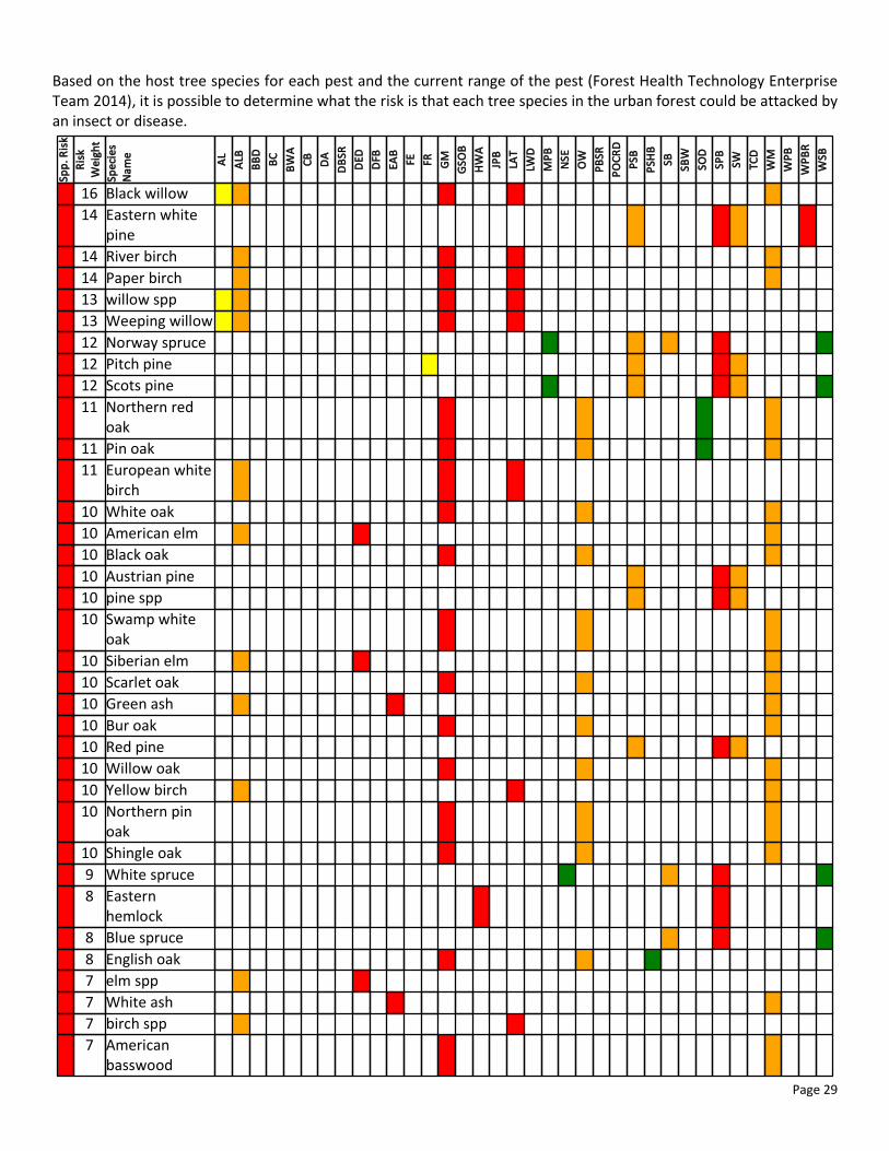
Based on the host tree species for each pest and the current range of the pest (Forest Health Technology EnterpriseTeam 2014), it is possible to determine what the risk is that each tree species in the urban forest could be attacked byan insect or disease.

Spp

. Ris

k

Ris

k

We

igh

t

Spe

cie

s

Na

me

AL

ALB

BB

D

BC

BW

A

CB

DA

DB

SR

DED

DFB

EAB

FE FR GM

GSO

B

HW

A

JPB

LAT

LWD

MP

B

NSE

OW

PB

SR

PO

CR

D

PSB

PSH

B

SB SBW

SOD

SPB

SW TCD

WM

WP

B

WP

BR

WSB

16 Black willow

14 Eastern whitepine

14 River birch

14 Paper birch

13 willow spp

13 Weeping willow

12 Norway spruce

12 Pitch pine

12 Scots pine

11 Northern redoak

11 Pin oak

11 European whitebirch

10 White oak

10 American elm

10 Black oak

10 Austrian pine

10 pine spp

10 Swamp whiteoak

10 Siberian elm

10 Scarlet oak

10 Green ash

10 Bur oak

10 Red pine

10 Willow oak

10 Yellow birch

10 Northern pinoak

10 Shingle oak

9 White spruce

8 Easternhemlock

8 Blue spruce

8 English oak

7 elm spp

7 White ash

7 birch spp

7 Americanbasswood

7 Chinese elm

7 oak spp

7 Smoothleaf elm

7 spruce spp

7 Sawtooth oak

7 Douglas fir

7 Boxelder

7 Commonchokecherry

6 Norway maple

6 Red maple

6 Sugar maple

6 Silver maple

6 Easterncottonwood

5 White fir

4 crabapple

4 Kousa dogwood

4 Floweringdogwood

4 'Bradford'callery pear

4 dogwood spp

4 hawthorn spp

4 European beech

4 Sweetgum

4 Littleleaf linden

4 Witch hazel

4 'Aristocrat'callery pear

4 Easternhophornbeam

4 American beech

4 Corneliancherry

4 cottonwoodspp

4 apple spp

4 Apricot

4 basswood spp

4 Crimean linden

4 pear spp

4 European alder

4 Smoke tree

4 ash spp

3 Black cherry

3 Japanese maple

3 Black walnut

3 Horse chestnut

3 Paperbarkmaple

3 Sycamoremaple

3 Hedge maple

3 Freeman maple

3 Katsura tree

3 Trident maple

3 Amur maple

3 maple spp

3 fir spp

3 Crimson kingnorway maple

3 Red sunset redmaple

3 buckeye spp

2 Sassafras

2 Spicebush

Note:Species that are not listed in the matrix are not known to be hosts to any of the pests analyzed.

Species Risk:• Red indicates that tree species is at risk to at least one pest within county• Orange indicates that tree species has no risk to pests in county, but has a risk to at least one pest within 250

miles from the county• Yellow indicates that tree species has no risk to pests within 250 miles of county, but has a risk to at least one

pest that is 250 and 750 miles from the county• Green indicates that tree species has no risk to pests within 750 miles of county, but has a risk to at least one

pest that is greater than 750 miles from the county

Risk Weight:Numerical scoring system based on sum of points assigned to pest risks for species. Each pest that could attack treespecies is scored as 4 points if red, 3 points if orange, 2 points if yellow and 1 point if green.

Pest Color Codes:• Red indicates pest is within New Haven county• Red indicates pest is within 250 miles county• Yellow indicates pest is within 750 miles of New Haven county• Green indicates pest is outside of these ranges

References

Abdollahi, K.K.; Ning, Z.H.; Appeaning, A., eds. 2000. Global climate change and the urban forest. Baton Rouge, LA:GCRCC and Franklin Press. 77 p.

Baldocchi, D. 1988. A multi-layer model for estimating sulfur dioxide deposition to a deciduous oak forest canopy.Atmospheric Environment. 22: 869-884.

Baldocchi, D.D.; Hicks, B.B.; Camara, P. 1987. A canopy stomatal resistance model for gaseous deposition to vegetatedsurfaces. Atmospheric Environment. 21: 91-101.

Bidwell, R.G.S.; Fraser, D.E. 1972. Carbon monoxide uptake and metabolism by leaves. Canadian Journal of Botany. 50:1435-1439.

British Columbia Ministry of Water, Land, and Air Protection. 2005. Residential wood burning emissions in BritishColumbia. British Columbia.

Broecker, W.S. 1970. Man's oxygen reserve. Science 168(3939): 1537-1538.

Bureau of Transportation Statistics. 2010. Estimated National Average Vehicle Emissions Rates per Vehicle by VehicleType using Gasoline and Diesel. Washington, DC: Burea of Transportation Statistics, U.S. Department ofTransportation. Table 4-43.

California Air Resources Board. 2013. Methods to Find the Cost-Effectiveness of Funding Air Quality Projects. Table 3Average Auto Emission Factors. CA: California Environmental Protection Agency, Air Resources Board.

Carbon Dioxide Information Analysis Center. 2010. CO2 Emissions (metric tons per capita). Washington, DC: The WorldBank.

Cardelino, C.A.; Chameides, W.L. 1990. Natural hydrocarbons, urbanization, and urban ozone. Journal of GeophysicalResearch. 95(D9): 13,971-13,979.

Ciesla, W. M.; Kruse, J. J. 2009. Large Aspen Tortrix. Forest Insect & Disease Leaflet 139. Washington, DC: U. S.Department of Agriculture, Forest Service. 8 p.

Clarke, S. R.; Nowak, J.T. 2009. Southern Pine Beetle. Forest Insect & Disease Leaflet 49. Washington, DC: U.S.Department of Agriculture, Forest Service. 8 p.

Connecticut Invasive Plant Working Group. 2013. Invasive Plant List. CT: University of Connecticut. <http://cipwg.uconn.edu/invasive_plant_list/>

Diller, J. D. 1965. Chestnut Blight. Forest Pest Leaflet 94. Washington, DC: U. S. Department of Agriculture, ForestService. 7 p.

Eastern Forest Environmental Threat Assessment Center. Dutch Elm Disease. http://threatsummary.forestthreats.org/threats/threatSummaryViewer.cfm?threatID=43

Energy Information Administration. 1994. Energy Use and Carbon Emissions: Non-OECD Countries. Washington, DC:Energy Information Administration, U.S. Department of Energy.

Energy Information Administration. 2013. CE2.1 Fuel consumption totals and averages, U.S. homes. Washington, DC:

Energy Information Administration, U.S. Department of Energy.

Energy Information Administration. 2014. CE5.2 Household wood consumption. Washington, DC: Energy InformationAdministration, U.S. Department of Energy.

Federal Highway Administration. 2013. Highway Statistics 2011.Washington, DC: Federal Highway Administration, U.S.Department of Transportation. Table VM-1.

Forest Health Technology Enterprise Team. 2014. 2012 National Insect & Disease Risk Maps/Data. Fort Collins, CO:U.S. Department of Agriculture, Forest Service. http://www.fs.fed.us/foresthealth/technology/nidrm2012.shtml

Georgia Forestry Commission. 2009. Biomass Energy Conversion for Electricity and Pellets Worksheet. Dry Branch, GA:Georgia Forestry Commission.

Heirigs, P.L.; Delaney, S.S.; Dulla, R.G. 2004. Evaluation of MOBILE Models: MOBILE6.1 (PM), MOBILE6.2 (Toxics), andMOBILE6/CNG. Sacramento, CA: National Cooperative Highway Research Program, Transportation Research Board.

Hirabayashi, S. 2011. Urban Forest Effects-Dry Deposition (UFORE-D) Model Enhancements, http://www.itreetools.org/eco/resources/UFORE-D enhancements.pdf

Hirabayashi, S. 2012. i-Tree Eco Precipitation Interception Model Descriptions, http://www.itreetools.org/eco/resources/iTree_Eco_Precipitation_Interception_Model_Descriptions_V1_2.pdf

Hirabayashi, S.; Kroll, C.; Nowak, D. 2011. Component-based development and sensitivity analyses of an air pollutantdry deposition model. Environmental Modeling and Software. 26(6): 804-816.

Hirabayashi, S.; Kroll, C.; Nowak, D. 2012. i-Tree Eco Dry Deposition Model Descriptions V 1.0

Houston, D. R.; O'Brien, J. T. 1983. Beech Bark Disease. Forest Insect & Disease Leaflet 75. Washington, DC: U. S.Department of Agriculture, Forest Service. 8 p.

Interagency Working Group on Social Cost of Carbon, United States Government. 2015. Technical Support Document:Technical Update of the Social Cost of Carbon for Regulatory Impact Analysis Under Executive Order 12866. http://www.whitehouse.gov/sites/default/files/omb/inforeg/scc-tsd-final-july-2015.pdf

Layton, M. 2004. 2005 Electricity Environmental Performance Report: Electricity Generation and Air Emissions. CA:California Energy Commission.

Leonardo Academy. 2011. Leonardo Academy's Guide to Calculating Emissions Including Emission Factors and EnergyPrices. Madison, WI: Leonardo Academy Inc.

Lovett, G.M. 1994. Atmospheric deposition of nutrients and pollutants in North America: an ecological perspective.Ecological Applications. 4: 629-650.

McPherson, E.G.; Maco, S.E.; Simpson, J.R.; Peper, P.J.; Xiao, Q.; VanDerZanden, A.M.; Bell, N. 2002. WesternWashington and Oregon Community Tree Guide: Benefits, Costs, and Strategic Planting. International Society ofArboriculture, Pacific Northwest, Silverton, OR.

McPherson, E.G.; Simpson, J.R. 1999. Carbon dioxide reduction through urban forestry: guidelines for professional andvolunteer tree planters. Gen. Tech. Rep. PSW-171. Albany, CA: U.S. Department of Agriculture, Forest Service, PacificSouthwest Research Station. 237 p.

McPherson, E.G.; Simpson, J.R.; Peper, P.J.; Crowell, A.M.N.; Xiao, Q. 2010. Northern California coast community treeguide: benefits, costs, and strategic planting. PSW-GTR-228. Gen. Tech. Rep. PSW-GTR-228. U.S. Department ofAgriculture, Forest Service, Pacific Southwest Research Station, Albany, CA.

McPherson, E.G.; Simpson, J.R.; Peper, P.J.; Gardner, S.L.; Vargas, K.E.; Maco, S.E.; Xiao, Q. 2006a. Coastal PlainCommunity Tree Guide: Benefits, Costs, and Strategic Planting PSW-GTR-201. USDA Forest Service, Pacific SouthwestResearch Station, Albany, CA.

McPherson, E.G.; Simpson, J.R.; Peper, P.J.; Gardner, S.L.; Vargas, K.E.; Xiao, Q. 2007. Northeast community tree guide:benefits, costs, and strategic planting.

McPherson, E.G.; Simpson, J.R.; Peper, P.J.; Maco, S.E.; Gardner, S.L.; Cozad, S.K.; Xiao, Q. 2006b. Midwest CommunityTree Guide: Benefits, Costs and Strategic Planting PSW-GTR-199. U.S. Department of Agriculture, Forest Service,Pacific Southwest Research Station, Albany, CA.

McPherson, E.G.; Simpson, J.R.; Peper, P.J.; Maco, S.E.; Gardner, S.L.; Vargas, K.E.; Xiao, Q. 2006c. PiedmontCommunity Tree Guide: Benefits, Costs, and Strategic Planting PSW-GTR 200. U.S. Department of Agriculture, ForestService, Pacific Southwest Research Station, Albany, CA.

McPherson, E.G.; Simpson, J.R.; Peper, P.J.; Maco, S.E.; Xiao Q.; Mulrean, E. 2004. Desert Southwest Community TreeGuide: Benefits, Costs and Strategic Planting. Phoenix, AZ: Arizona Community Tree Council, Inc. 81 :81.

McPherson, E.G.; Simpson, J.R.; Peper, P.J.; Scott, K.I.; Xiao, Q. 2000. Tree Guidelines for Coastal Southern CaliforniaCommunities. Local Government Commission, Sacramento, CA.

McPherson, E.G.; Simpson, J.R.; Peper, P.J.; Xiao, Q. 1999. Tree Guidelines for San Joaquin Valley Communities. LocalGovernment Commission, Sacramento, CA.

McPherson, E.G.; Simpson, J.R.; Peper, P.J.; Xiao, Q.; Maco, S.E.; Hoefer, P.J. 2003. Northern Mountain and PrairieCommunity Tree Guide: Benefits, Costs and Strategic Planting. Center for Urban Forest Research, USDA Forest Service,Pacific Southwest Research Station, Albany, CA.

McPherson, E.G.; Simpson, J.R.; Peper, P.J.; Xiao, Q.; Pittenger, D.R.; Hodel, D.R. 2001. Tree Guidelines for InlandEmpire Communities. Local Government Commission, Sacramento, CA.

Michigan State University. 2010. Emerald ash borer. East Lansing, MI: Michigan State University [and others].

Mielke, M. E.; Daughtrey, M. L. How to Identify and Control Dogwood Anthracnose. NA-GR-18. Broomall, PA: U. S.Department of Agriculture, Forest Service, Northeastern Area and Private Forestry.

Murray, F.J.; Marsh L.; Bradford, P.A. 1994. New York State Energy Plan, vol. II: issue reports. Albany, NY: New YorkState Energy Office.

National Invasive Species Information Center. 2011. Beltsville, MD: U.S. Department of Agriculture, National InvasiveSpecies Information Center. http://www.invasivespeciesinfo.gov/plants/main.shtml

Nicholls, T. H.; Anderson, R. L. 1977. How to Identify White Pine Blister Rust and Remove Cankers. St. Paul, MN: U.S.Department of Agriculture, Forest Service, Northeastern Area State and Private Forestry

Northeastern Area State and Private Forestry. 1998. How to identify and manage Dutch Elm Disease. NA-PR-07-98.

Newtown Square, PA: U.S. Department of Agriculture, Forest Service, Northeastern Area State and Private Forestry.

Northeastern Area State and Private Forestry. 2005. Gypsy moth digest. Newtown Square, PA: U.S. Department ofAgriculture, Forest Service, Northeastern Area State and Private Forestry.

Nowak, D.J. 1994. Atmospheric carbon dioxide reduction by Chicago’s urban forest. In: McPherson, E.G.; Nowak, D.J.;Rowntree, R.A., eds. Chicago’s urban forest ecosystem: results of the Chicago Urban Forest Climate Project. Gen. Tech.Rep. NE-186. Radnor, PA: U.S. Department of Agriculture, Forest Service, Northeastern Forest Experiment Station:83-94.

Nowak, D.J. 1995. Trees pollute? A "TREE" explains it all. In: Proceedings of the 7th National Urban ForestryConference. Washington, DC: American Forests: 28-30.

Nowak, D.J. 2000. The interactions between urban forests and global climate change. In: Abdollahi, K.K.; Ning, Z.H.;Appeaning, A., eds. Global Climate Change and the Urban Forest. Baton Rouge, LA: GCRCC and Franklin Press: 31-44.

Nowak, D.J., Hirabayashi, S., Bodine, A., Greenfield, E. 2014. Tree and forest effects on air quality and human health inthe United States. Environmental Pollution. 193:119-129.

Nowak, D.J., Hirabayashi, S., Bodine, A., Hoehn, R. 2013. Modeled PM2.5 removal by trees in ten U.S. cities andassociated health effects. Environmental Pollution. 178: 395-402.

Nowak, D.J.; Civerolo, K.L.; Rao, S.T.; Sistla, S.; Luley, C.J.; Crane, D.E. 2000. A modeling study of the impact of urbantrees on ozone. Atmospheric Environment. 34: 1601-1613.

Nowak, D.J.; Crane, D.E. 2000. The Urban Forest Effects (UFORE) Model: quantifying urban forest structure andfunctions. In: Hansen, M.; Burk, T., eds. Integrated tools for natural resources inventories in the 21st century.Proceedings of IUFRO conference. Gen. Tech. Rep. NC-212. St. Paul, MN: U.S. Department of Agriculture, ForestService, North Central Research Station: 714-720.

Nowak, D.J.; Crane, D.E.; Dwyer, J.F. 2002a. Compensatory value of urban trees in the United States. Journal ofArboriculture. 28(4): 194 - 199.

Nowak, D.J.; Crane, D.E.; Stevens, J.C.; Hoehn, R.E. 2005. The urban forest effects (UFORE) model: field data collectionmanual. V1b. Newtown Square, PA: U.S. Department of Agriculture, Forest Service, Northeastern Research Station, 34p. http://www.fs.fed.us/ne/syracuse/Tools/downloads/UFORE_Manual.pdf

Nowak, D.J.; Crane, D.E.; Stevens, J.C.; Ibarra, M. 2002b. Brooklyn’s urban forest. Gen. Tech. Rep. NE-290. NewtownSquare, PA: U.S. Department of Agriculture, Forest Service, Northeastern Research Station. 107 p.

Nowak, D.J.; Dwyer, J.F. 2000. Understanding the benefits and costs of urban forest ecosystems. In: Kuser, John, ed.Handbook of urban and community forestry in the northeast. New York, NY: Kluwer Academics/Plenum: 11-22.

Nowak, D.J.; Hoehn, R.; Crane, D. 2007. Oxygen production by urban trees in the United States. Arboriculture & UrbanForestry. 33(3):220-226.

Nowak, D.J.; Hoehn, R.E.; Crane, D.E.; Stevens, J.C.; Walton, J.T; Bond, J. 2008. A ground-based method of assessingurban forest structure and ecosystem services. Arboriculture and Urban Forestry. 34(6): 347-358.

Nowak, D.J.; Stevens, J.C.; Sisinni, S.M.; Luley, C.J. 2002c. Effects of urban tree management and species selection onatmospheric carbon dioxide. Journal of Arboriculture. 28(3): 113-122.

Ostry, M.E.; Mielke, M.E.; Anderson, R.L. 1996. How to Identify Butternut Canker and Manage Butternut Trees. U. S.Department of Agriculture, Forest Service, North Central Forest Experiment Station.

Peper, P.J.; McPherson, E.G.; Simpson, J.R.; Albers, S.N.; Xiao, Q. 2010. Central Florida community tree guide: benefits,costs, and strategic planting. Gen. Tech. Rep. PSW-GTR-230. U.S. Department of Agriculture, Forest Service, PacificSouthwest Research Station, Albany, CA.

Peper, P.J.; McPherson, E.G.; Simpson, J.R.; Vargas, K.E.; Xiao Q. 2009. Lower Midwest community tree guide: benefits,costs, and strategic planting. PSW-GTR-219. Gen. Tech. Rep. PSW-GTR-219. U.S. Department of Agriculture, ForestService, Pacific Southwest Research Station, Albany, CA.

U.S. Environmental Protection Agency. 2010. Light-Duty Vehicle Greenhouse Gas Emission Standards and CorporateAverage Fuel Economy Standards. Washington, DC: U.S. Environmental Protection Agency. EPA-420-R-10-012a

U.S. Environmental Protection Agency. 2015. The social cost of carbon. http://www.epa.gov/climatechange/EPAactivities/economics/scc.html

U.S. Forest Service. 2005. Hemlock Woolly Adelgid. Pest Alert. NA-PR-09-05. Newtown Square, PA: U. S. Departmentof Agriculture, Forest Service, Northern Area State and Private Forestry.

van Essen, H.; Schroten, A.; Otten, M.; Sutter, D.; Schreyer, C.; Zandonella, R.; Maibach, M.; Doll, C. 2011. ExternalCosts of Transport in Europe. Netherlands: CE Delft. 161 p.

Vargas, K.E.; McPherson, E.G.; Simpson, J.R.; Peper, P.J.; Gardner, S.L.; Xiao, Q. 2007a. Interior West Tree Guide.

Vargas, K.E.; McPherson, E.G.; Simpson, J.R.; Peper, P.J.; Gardner, S.L.; Xiao, Q. 2007b. Temperate Interior WestCommunity Tree Guide: Benefits, Costs, and Strategic Planting.

Vargas, K.E.; McPherson, E.G.; Simpson, J.R.; Peper, P.J.; Gardner, S.L.; Xiao, Q. 2008. Tropical community tree guide:benefits, costs, and strategic planting. PSW-GTR-216. Gen. Tech. Rep. PSW-GTR-216. U.S. Department of Agriculture,Forest Service, Pacific Southwest Research Station, Albany, CA.

Worrall, J.J. 2007. Chestnut Blight. Forest and Shade Tree Pathology.http://www.forestpathology.org/dis_chestnut.html

Zinke, P.J. 1967. Forest interception studies in the United States. In: Sopper, W.E.; Lull, H.W., eds. Forest Hydrology.Oxford, UK: Pergamon Press: 137-161.

i-tree ecosystem analysis - yale university

Documents