Page 1 of 16

IBIL setup operation manual

for SynerJY® software version 1.8.5.0

Manual version 1.0, 31/10/2008

Author: Carlos Marques

Equipment Managers: Carlos Marques, +351219946084, cmarques@itn.pt

Luís Alves, +351219946112, lcalves@itn.pt

Instituto Tecnológico e Nuclear

Unidade de Física e de Aceleradores

Page 2 of 16

Page 3 of 16

General description

The IBIL setup is comprised of a monochromator (TRIAX®

190), to which a Peltier cooled CCD

detector (Symphony®

1024×256 pixel) is coupled, and a cooling unit, as shown in figure 1. From

the monochromator to the experimental chamber goes an optical fiber and a coupling and focusing

device, detailed in fig. 2. The connections are numbered, each pair cable – socket is univocally

identified with the same number, from 1 to 7.

The available range of measurement is from 200 nm to 1100 nm, with 0.3 nm resolution in the

optimum combination of diffraction grating and entrance slit width (software controlled, from 0.002

mm to 2 mm). There are manually switchable filters (cutting up to 385 nm – top filter - and up to

630 nm – bottom filter, with the central position empty) at the entrance of the monochromator.

Figure 1 – Image of the IBIL setup, with the optical fiber attached to the experimental chamber via

mirror based coupling device.

monochromator

optical fiber

CCD power and

cooling unit

sample position

control knobs

filter manual

slide

CCD

Page 4 of 16

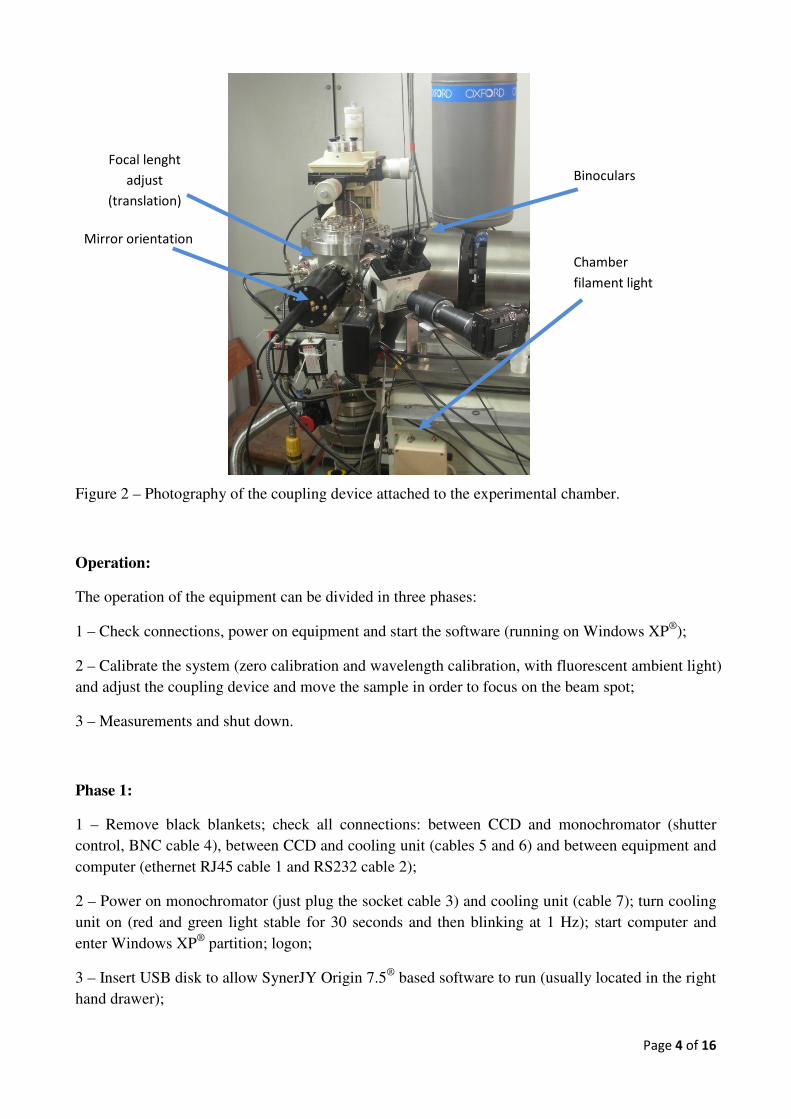
Figure 2 – Photography of the coupling device attached to the experimental chamber.

Operation:

The operation of the equipment can be divided in three phases:

1 – Check connections, power on equipment and start the software (running on Windows XP®

);

2 – Calibrate the system (zero calibration and wavelength calibration, with fluorescent ambient light)

and adjust the coupling device and move the sample in order to focus on the beam spot;

3 – Measurements and shut down.

Phase 1:

1 – Remove black blankets; check all connections: between CCD and monochromator (shutter

control, BNC cable 4), between CCD and cooling unit (cables 5 and 6) and between equipment and

computer (ethernet RJ45 cable 1 and RS232 cable 2);

2 – Power on monochromator (just plug the socket cable 3) and cooling unit (cable 7); turn cooling

unit on (red and green light stable for 30 seconds and then blinking at 1 Hz); start computer and

enter Windows XP®

partition; logon;

3 – Insert USB disk to allow SynerJY Origin 7.5®

based software to run (usually located in the right

hand drawer);

Mirror orientation

Focal lenght

adjust

(translation)

Binoculars

Chamber

filament light

Page 5 of 16

4 – Double click on SynerJY®

icon located at the computer desktop;

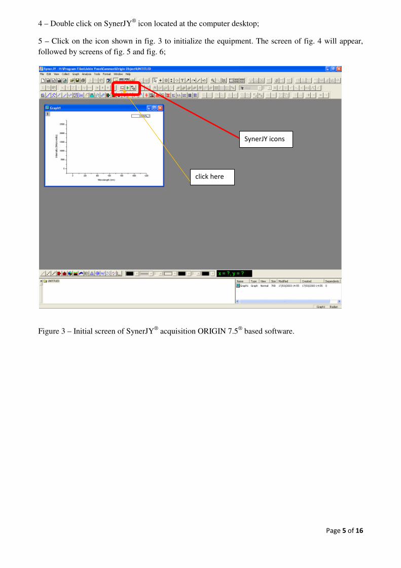
5 – Click on the icon shown in fig. 3 to initialize the equipment. The screen of fig. 4 will appear,

followed by screens of fig. 5 and fig. 6;

Figure 3 – Initial screen of SynerJY®

acquisition ORIGIN 7.5®

based software.

click here

SynerJY icons

Page 6 of 16

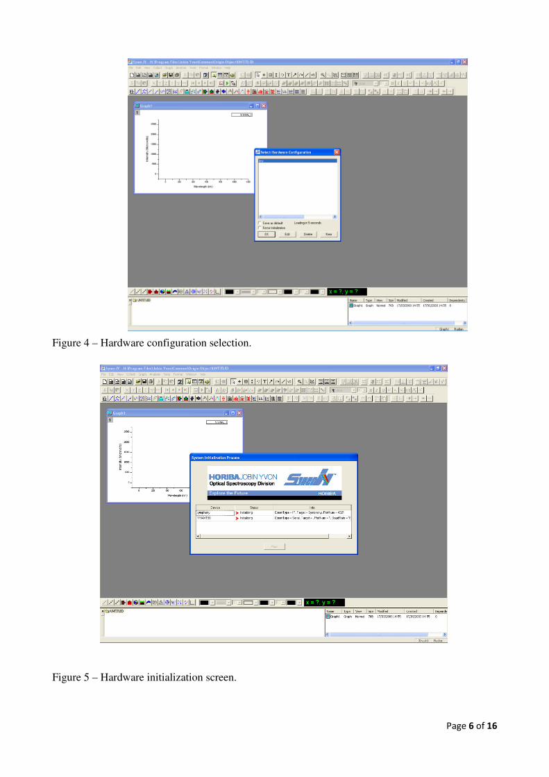
Figure 4 – Hardware configuration selection.

Figure 5 – Hardware initialization screen.

Page 7 of 16

Figure 6 – Acquisition menu, for wavelength range selection, as well as acquisition or exposure

time.

6 – Check temperature, selecting ADVANCED on the screen of fig. 6. Fig. 7 screen will show up;

wait for T < 204 K to start acquisition (about 10 minutes) and click OK;

Figure 7 – Temperature check. This menu also allows cosmic ray removal (removes intense and

narrow peaks) and background correction (removes baseline noise, which is 1240 ± 10 counts,

check it with the shutter closed on the PREVIEW screen, fig. 11).

temperature

Page 8 of 16

If you got up to this screen and T is about 202 K – 204 K then proceed to phase 2. Lights on the

cooling unit should both be green and stable.

Phase 2

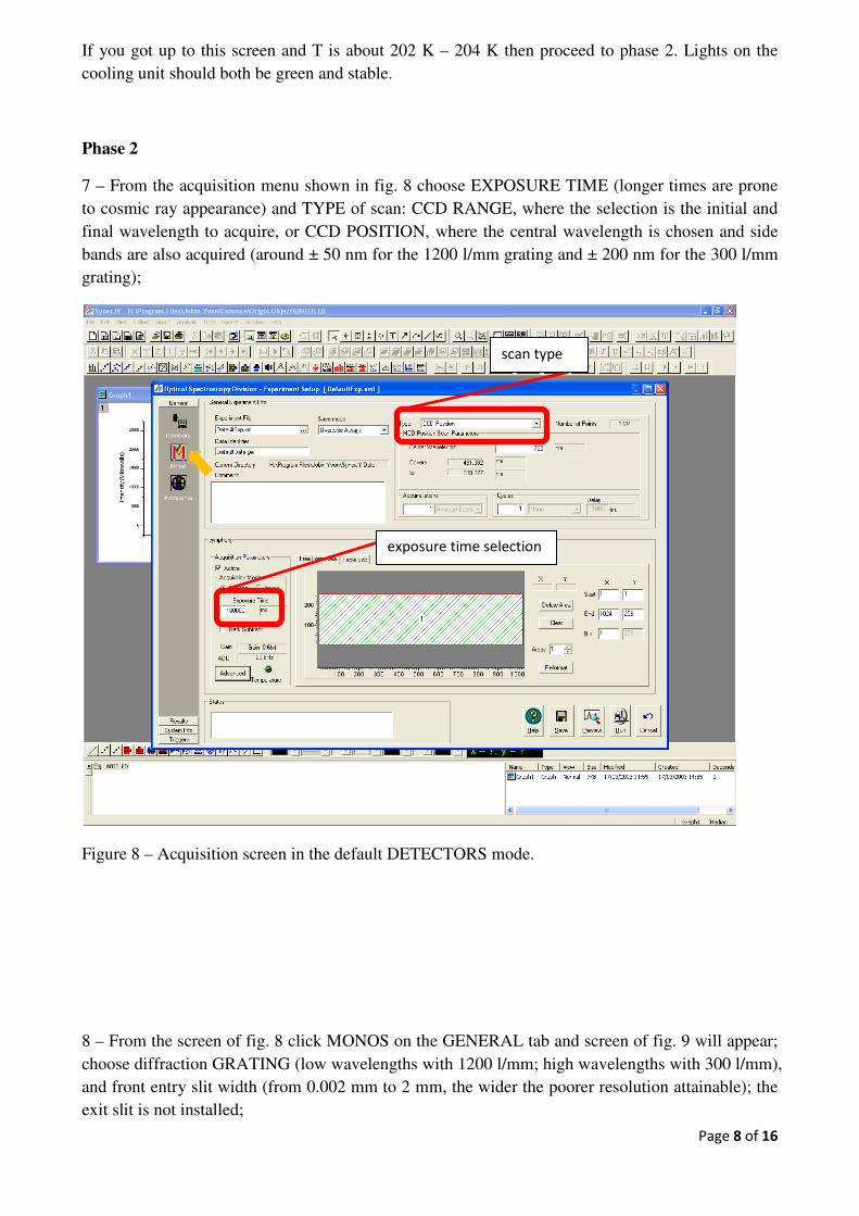
7 – From the acquisition menu shown in fig. 8 choose EXPOSURE TIME (longer times are prone

to cosmic ray appearance) and TYPE of scan: CCD RANGE, where the selection is the initial and

final wavelength to acquire, or CCD POSITION, where the central wavelength is chosen and side

bands are also acquired (around ± 50 nm for the 1200 l/mm grating and ± 200 nm for the 300 l/mm

grating);

Figure 8 – Acquisition screen in the default DETECTORS mode.

8 – From the screen of fig. 8 click MONOS on the GENERAL tab and screen of fig. 9 will appear;

choose diffraction GRATING (low wavelengths with 1200 l/mm; high wavelengths with 300 l/mm),

and front entry slit width (from 0.002 mm to 2 mm, the wider the poorer resolution attainable); the

exit slit is not installed;

exposure time selection

scan type

Page 9 of 16

Figure 9 – Acquisition screen in the MONOS mode, allowing choosing the grating and slit width.

Figure 10 – Photography of the optical fiber

in the test position to calibrate the system and

monitor its sensitivity; also in the picture is

the beam current meter.

9 – With the optical fiber in the test position (fig. 10) perform an acquisition of light from the

fluorescent lamp and check peak positions; from screens of fig. 8 or fig. 9, click PREVIEW, screen

in figure 11 appears;

grating selection

slit width selection

Page 10 of 16

Figure 11 – Preview menu, in DETECTORS default, with a 0 order preview acquisition.

10 - Zero order calibration: position at 0 nm and acquire (choosing 0.002 mm entrance slit width

and appropriate exposure time in order not to saturate the CCD, which happens over 65536 – or 16

bit - counts) by clicking RUN; a Gaussian shaped band should appear centered at 0 nm; calibrate if

peak position is different (step 11); adjust CCD and the entrance of the optical fiber if band is not

Gaussian (refer to Jobin Yvon manual); repeat for the other grating;

11 – If the peak is not centered at 0 nm, click MONOS on screen of fig. 11 and the screen of fig. 12

will appear. Next, click CALIBRATE and fig. 13 shows the expected screen. To the CURRENT

POSITION wavelength value subtract the measured peak center (if this is negative… add) and input

this value on the CALIBRATED POSITION field. Click OK and acquire new spectra; Repeat this

step if zero order is not centered at 0 nm. Repeat for the other grating;

cursor coordinates

selection

Page 11 of 16

Figure 12 – Preview screen in the MONOS mode.

Figure 13 – Zero calibration; to the current position subtract the desired peak value.

Page 12 of 16

12 – Wavelength calibration: acquire a spectrum centered at 550 nm (to monitor Hg line at 546 nm,

FWHM about 0.4 nm), again for both gratings, (fig. 14) and confirm that the bands in table 1 are

found in their expected positions. Choose exposure times and entrance slit width in order not to

saturate the CCD; use top filter to avoid 2nd

order diffractions;

Figure 14 – Typical emission lines present in common fluorescent lamps.

Table 1 – Most intense Hg+ emission lines (CRC Handbook).

13 – Focus on the beam spot: input the coupling mirror based device with a laser beam; from the

binoculars check the laser spot on the sample and make it coincide with the beam spot by adjusting

the sample position and the optical coupling (cf. fig. 1);

14 – Reconnect the optical fiber to the coupling device; cover the binoculars and the equipment

with the black blanket, but allowing for CCD ventilation;

Emission lines of Hg+, present in typical fluorescent lamps

wavelength (nm) relative intensity wavelength (nm) relative intensity

184.95 1000 407.78 150

253.65 15000 433.92 250

265.20 250 434.75 400

265.37 400 435.83 4000

289.36 150 546.07 1100

296.73 1200 567.59 160

302.15 300 576.92 240

312.57 400 578.97 100

313.16 320 579.07 280

313.18 320 580.38 140

365.02 2800 690.75 250

365.48 300 708.19 250

366.33 240 709.19 250

404.66 1800 1013.97 2000

Page 13 of 16

Phase 3

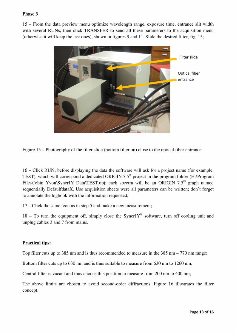
15 – From the data preview menu optimize wavelength range, exposure time, entrance slit width

with several RUNs; then click TRANSFER to send all these parameters to the acquisition menu

(otherwise it will keep the last ones), shown in figures 9 and 11. Slide the desired filter, fig. 15;

Figure 15 – Photography of the filter slide (bottom filter on) close to the optical fiber entrance.

16 – Click RUN; before displaying the data the software will ask for a project name (for example:

TEST), which will correspond a dedicated ORIGIN 7.5®

project in the program folder (H:\Program

Files\Jobin Yvon\SynerJY Data\TEST.opj; each spectra will be an ORIGIN 7.5®

graph named

sequentially DefaulfdataX. Use acquisition sheets were all parameters can be written; don’t forget

to annotate the logbook with the information requested;

17 – Click the same icon as in step 5 and make a new measurement;

18 – To turn the equipment off, simply close the SynerJY®

software, turn off cooling unit and

unplug cables 3 and 7 from mains.

Practical tips:

Top filter cuts up to 385 nm and is thus recommended to measure in the 385 nm – 770 nm range;

Bottom filter cuts up to 630 nm and is thus suitable to measure from 630 nm to 1260 nm;

Central filter is vacant and thus choose this position to measure from 200 nm to 400 nm;

The above limits are chosen to avoid second-order diffractions. Figure 16 illustrates the filter

concept.

Filter slide

Optical fiber

entrance

Page 14 of 16

Figure 16 – Luminescence spectra of a fluorescent lamp acquired with the 385 nm or the 630 nm

filter. The use of the filter prevents some 2nd

order diffractions and while the 385 nm inhibits these

diffractions up to 770 nm (and thus allow the 404 nm 2nd

diffraction at 808 nm, cf. table 1) the 630

nm filter extends this effect up to 1260 nm.

Use black blankets to avoid stray light, covering essentially the monochromator and filter region, as

well as the CCD connection (do not cover the entire CCD or the temperature will not drop to 203

K). Don’t forget to cover also the binoculars.

Take one spectra without beam in the experimental conditions used to ascertain the absence of any

system related features.

Take one spectra with the minimum of ambient light possible to exclude the appearance of external

light features on the spectra.

Considering the efficiency curves of the 1200 l/mm and 300 l/mm gratings (fig. 17) the first should

be used for the lower wavelengths while the latter used for higher ones. Each grating has a

maximum or blaze wavelength, 250 nm for the 1200 l/mm and 1000 nm for the 300 l/mm.

760 770 780 790 800 810 820 830 840

2000

3000

4000

5000 fluorescent lamp, CCD position 800 nm, 1200 l/mm

slit 0.002 mm, time 10 s

Inte

nsity (

Cou

nts

)

Wavelength (nm)

385 nm cut

630 nm cut

2nd

order

from 404 nm

appears

at 808 nm

Page 15 of 16

Figure 17 – Theoretical spectral efficiency curves for a) 300 grooves/mm (transversal electric, TE,

and transversal magnetic, TM) and b) 1200 grooves/mm, used in our system.

Step 12 should be repeated for every sample or spot analysed.

The usable wavelength range is dictated by the efficiency of the CCD, fig. 18.

Figure 18 –CCD spectral sensitivity at RT.

a)

b)

CCD detectable range

Page 16 of 16

Troubleshooting…

You don’t get the screen shown in figure 6: check connections between PC and equipment (cables 1

and 2);

The temperature doesn’t reach 203 K: check if CCD ventilation is not obstructed;

The noise level is higher than 1240 counts: check CCD temperature and block stray light.

User Notes:

Manual available online at http://www.itn.pt/facilities/lfi/manual_ibil.pdf