ibm spss predictive analytics workshop spss predictive analytics workshop ... 1.8 from the drop-down...

IBM SPSS Predictive Analytics Workshop

Workbook – Commercial Edition

2014

Contents Page 1

Contents

P1. PREDICTIVE IN 20 MINUTES ..................................................................................................................................... 3 1. FINDING PATTERNS AND GROUPS ......................................................................................................................... 23 2. UNDERSTANDING THE PAST, PREDICTING THE FUTURE ......................................................................................... 32 3. OPTIMIZE DECISIONS ............................................................................................................................................. 53

Overview

This hands-on IBM SPSS Predictive Analytics Workshop is an instructor-led session using IBM’s data mining and predictive modeling software and is designed for those who are familiar with predictive analytics, as well as for beginners. Through this workshop you will experience firsthand how IBM SPSS Modeler works and how easy it is to implement predictive analytics.

Predictive in 20 Minutes

P1. Start Modeler if it’s not already open. P2. From the Sources palette, double-click on the Statistics File node to add it to the canvas.

P3. Double-click the Statistics File node to open a dialog box. Use the data tab to import the CustomerData.sav file from C:\ModelerWorkshop\Predictivein20Minutes\CustomerData.sav. Click on the Preview button at the top of the dialog box to see the first 10 records in the file.

P4. This is an extraction of data from a retail company’s CRM system. It includes data related to customers’ demographic, purchasing behavior, segment, and marketing campaign response.

P5. After reviewing the output from the Table node, click on the red X to close.

P6. From the Graphs palette, add a distribution node to the canvas and connect it to the data source using any of the following methods:

Double-click on the node in the palette to automatically add it to the stream and join it to the selected node.

Drag and drop the node from out of the palette and on to the canvas. Select the first node, right-click and select Connect from the context menu, and then left-click on the second node to connect it.

Click and hold the middle mouse button on the first node, move the cursor to the second node and release when the cursor is on top of the second node.

Double-click to edit the Distribution node, choose Response from the Field drop down menu, and select Run.

P7. The resulting graph shows that of the 2070 customers in this dataset, only 38.84%, or 804 customers, responded to the campaign. The remaining 61.16%, or 1266 customers, did not respond. Our goal, then, is to build a model to understand the relationships within the data that lent themselves to customer response.

P8. From the Field Ops palette, add a Type node to the canvas and connect it to the data source.

P9. Double-click on the Type node and click the Read Values button to scan the data as well as to display and update the range of values. Modify the Role of ID to Record ID and the Response field to Target. The Measurement of our Target should be set to Flag, which reflects two potential Values: Responded or Did not Respond. The remaining variables will remain as Inputs in our analysis.

P10. From the Output palette, double-click on the Data Audit node and connect it to the Type node. Right-click to select Run or chose the Run Selection button on the toolbar.

P11. In the Audit tab of the resulting output, thumbnail graphs, storage icons, and summary statistics for all fields can be found. Double-clicking on any of the graphs will provide a more detailed outlook of the variable In the Quality tab (not shown), information about outliers, extremes and missing values are shown.

P12. From the Graphs palette, select the Web node and connect it to the Type node. Double-click the Web node to edit the settings. Choose Directed web and select Response in the To Field drop down. Add the remaining fields in the From Fields drop down, and select Run.

P13. The output of this exploratory visualization shows the strength of relationships between values of two or more fields, displayed with varying line types to indicate increasing strength. Using the sliders under the graph to change the view reveals, for example, that individuals with a status type of single responded to the campaign 466 times.

P14. After reviewing the output, click on the red X to close.

P15. Now that we have explored our data, we can build a model to uncover the key drivers resulting in campaign response. We will do this by selecting the CHAID node from the Modeling palette and connecting it to the Type node.

P16. Double-click on the CHAID node to review the settings. Since we have already declared Response as our Target variable, the settings are automatically defined as defaults. Select Run.

P17. The CHAID model is automatically generated and added to our canvas. Double-click on the generated model to review the output.

P18. In the Model tab of the resulting output, we are provided with a list of the most important predictors of campaign response; the first few being Region, Status and Age; as well as rules for the model.

P19. The Viewer tab shows the CHAID tree, reflecting the cut points of the important predictors as determined by the model. Following a branch down, we are able to discover key insights. For example; customers between 20 and 26 years of age, with between 4 and 14 transactions in the current year, who lived in Region 1 or 2; responded to the campaign at very high rates.

P20. From the Output palette, add a Table node to the canvas and connect it to the CHAID model node. Run the Table by right-clicking and selecting Run, or by using the Run Selection toolbar button.

P21. Look at the last three columns of the table. The third from the last is the actual outcome, whether or not the customer responded to the campaign; the second to last column contains the predicted outcomes; and the last column is the confidence of that prediction. For example, the first record shows a customer who did, in fact, respond to a campaign. The appended columns show that the model predicted that the customer would respond with 98% confidence.

P22. To see the overall accuracy of the model, select an Analysis node from the Output palette, connect it to the generated model, and select Run.

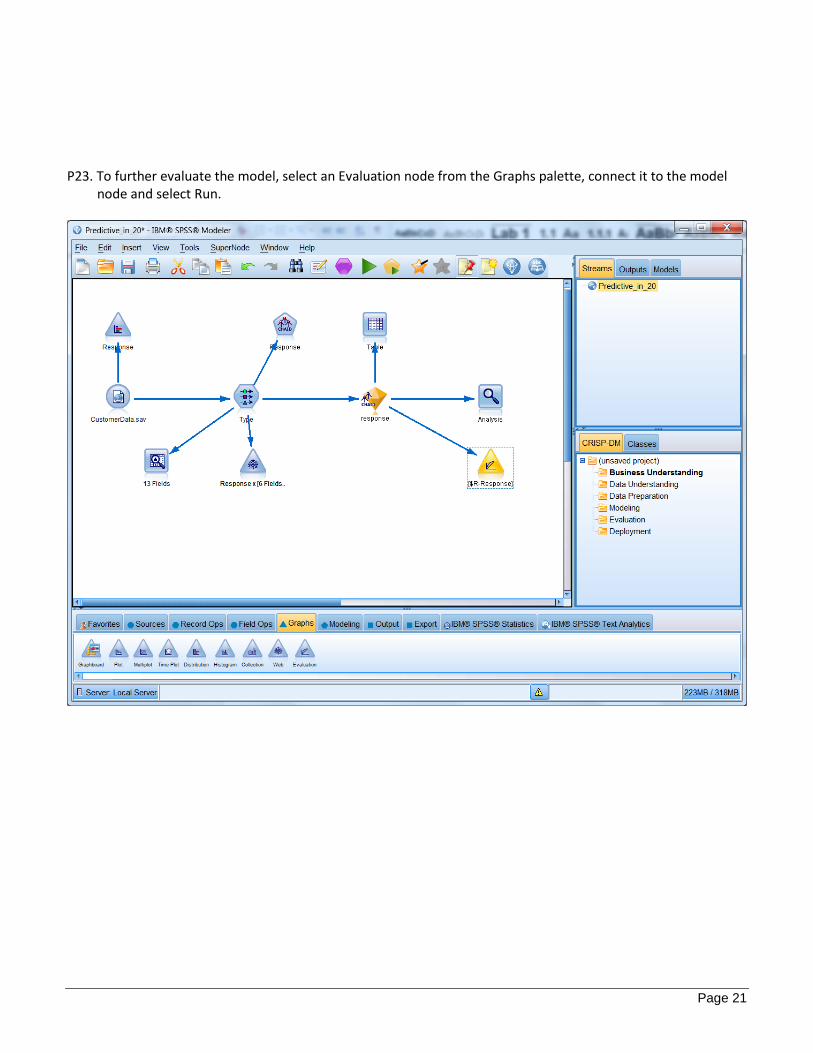
P23. To further evaluate the model, select an Evaluation node from the Graphs palette, connect it to the model node and select Run.

P24. In the resulting gains chart, the red line reflects what you could expect without Predictive Analytics. The blue line; however, reflects the gain in response you could achieve utilizing Predictive Analytics. Therefore, if you were to randomly select 50% of your client base, you could expect to have captured 50% of those likely to respond. By using Predictive Analytics, you can more effectively target those 50% of clients and capture almost 90% of those likely to respond.

Using IBM SPSS Modeler, you can more decisively target your client base to capture a greater proportion who are likely to respond. Predictive Analytics, then, gives you the capability to move squarely out of a “Sense and Respond” mode and into one of predicting and taking precise action.

P25. Save the stream to your local directory before closing it.

1. Finding Patterns and Groups

1.1 Open the Customer Segmentation.str file from the workshop directory. In IBM SPSS Modeler, click on File, Open stream, and then navigate to C:\Modeler Workshop\Clustering Stream. Either double-click on Customer Segmentation.str, or select it and then click on Open.

You might recall that in the Predictive in 20 exercise there was a field assigning each customer to a marketing cluster or segment. We're going to take a step back in our story to take a deeper look at how that is accomplished in IBM SPSS Modeler. We will be joining two data files together; one file contains customer transaction data, and exists in a database, while the other file is an Excel file and contains customer demographics. Though the files are in different formats, the Merge node in IBM SPSS Modeler can very easily join the files without first requiring the analyst to translate one file and/or the other into the same format. For ease during this workshop, the two source nodes on the canvas, and the merge node used to join them together, have already been configured and connected for you.

1.2 From the Output palette, add a Table node to the canvas and connect it to the Merge node.

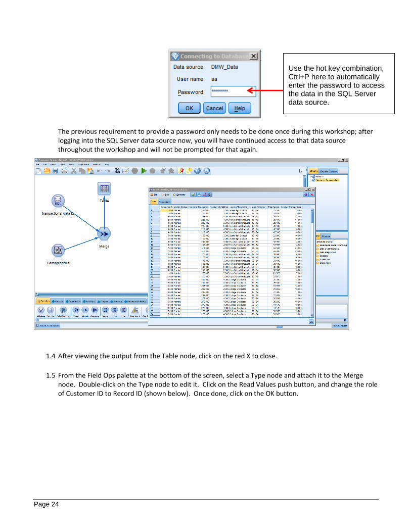
1.3 Once connected, right click on the Table node and select Run to review the data after having been merged. If prompted for a password, use “Ctrl+P” to automatically populate the password.

The previous requirement to provide a password only needs to be done once during this workshop; after logging into the SQL Server data source now, you will have continued access to that data source throughout the workshop and will not be prompted for that again.

1.4 After viewing the output from the Table node, click on the red X to close.

1.5 From the Field Ops palette at the bottom of the screen, select a Type node and attach it to the Merge

node. Double-click on the Type node to edit it. Click on the Read Values push button, and change the role of Customer ID to Record ID (shown below). Once done, click on the OK button.

Use the hot key combination, Ctrl+P here to automatically enter the password to access the data in the SQL Server data source.

At this point we are ready to cluster the cases into segments. For this we’ll use the two-Step clustering engine.

1.6 From the Modeling palette select the Two Step modeling node and attach it to the Type node. Double-

click on the Two Step node to edit it. In the Model tab, change the maximum number of clusters from 15 to 4, (shown below). Once done, click on the Run button.

v

1.7 Double-click on the model nugget to view the results of the cluster analysis in the Cluster Viewer.

As we specified, the Two Step clustering engine resolved into 4 clusters. Looking at the Cluster Quality measure in the left panel, we see that the Silhouette measure (which is a measure of the clusters’ internal cohesion as well as how well they exclude dissimilar cases) is fair, with a value of just under 0.5. Such results are not atypical, but may also suggest that fewer and/or other variables might be needed to increase the Silhouette value. On the right side of the viewer is a pie chart illustrating the cluster sizes.

1.8 From the drop-down menu in the right viewer select Predictor Importance.

Now the right side of the viewer displays a graph with the variables ranked in order of importance for cluster definition. We can see that Level of Education is the most important variable, followed by Marital Status.

1.9 Now, from the drop-down menu in the left viewer, select Clusters; from the drop-down menu in the right viewer, select Cell Distribution. (Shown below in red).

v v

The left panel of the Viewer displays the clusters in order of their size, left to right. The darkness of the shading of each variable indicates its importance in cluster definition; the lighter the shading, the less important is the variable in defining the clusters.

1.10 Click on any cell in the grid in the left panel to view in the right panel how a cluster distribution

compares to the remaining clusters. 1.11 Click in the left panel on the heading for Cluster-2 and then hold the shift key on your keyboard

and simultaneously click on the heading for cluster-4. This selects the entire table. The right

panel will display the Cluster Comparison view, which displays the variable distributions relative

to each selected cluster.

1.12 After reviewing the Cluster Viewer, click on the red X to close and return to the Modeler workbench.

1.13 From the Field Ops palette, drag a Reclassify node onto the canvas and connect it to the model

node (nugget).

1.14 Double-click on the Reclassify node to edit it.

In the Settings tab of the Reclassify dialog, use the drop-down menu to select the variable $T-TwoStep as the field to be reclassified. Select “Existing Field.” Select “Get.” Enter the new values which better describe the clusters (an example is shown below, but you can enter your own labels as desired).

1.15 Click Okay.

1.16 From the Output palette, drag a Table node onto the workbench and connect it to the Reclassify

node. Once connected, right-click on the Table node and select Run.

The resulting table now includes a new column with the cluster assignments. You can also export these results back into the original data set or into other formats for use in later analyses. The following stream illustrates this, though we will not construct it here. Instead, for the purposes of this workshop, this step was already done and the data exported using the SQL Export node (below).

2. Understand the Past, Predict the Future

2.1 Open the “Predictive Marketing Response Stream.str” file from the workshop directory. In IBM SPSS Modeler, click on File, Open stream, and then navigate to C:\Modeler Workshop\Classification Stream. Either double-click on Predictive Marketing Response Stream.str, or select it and then click on Open.

For the purposes of this workshop, this excercise begins with a stream that has already been partially constructed. Note in particular that we are using the same customer data from the Predictive in 20 exercise. Notice also that we will be using unstructured data in the form of customer comments, and contained in a Microsoft Excel .xls file.

2.2 From the Record Opps palette, a Merge node has already been placed on the canvas. Double-click on the Merge node to review the settings. You’ll notice that the two data sources on the canvas are being joined by a common Key, in this case ID. Select Preview to see the first 10 records of this new merge.

2.3 Scrolling to the right, you will notice the assigned cluster for each customer, created in the previous exercise;

and a newly merged column, containing unstructured customer comments. Click OK to close.

2.4 After the merge, we’ve attached a Type node to read (or “instantiate”) the data and define the measurement level and role of each variable in the analysis. Double-click on the Type node to review its settings. Notice that, as in the Predictive in 20 exercise, Response is our Target variable. An additional input, Comments, has been added as a result of the merge. For now, click on either OK or Cancel to close this dialog.

Using Text Analytics, we can identify patterns in the unstructured data and from them, create categories which contain the ideas and sentiments as expressed by our clients.

2.5 From the IBM SPSS Text Analytics palette, add a Text mining node to the canvas, and connect it to the Type node. Double-click on the Text Mining node to review its settings. Using the Text Field drop down, select Comments.

2.6 Select the Model tab and scroll down to the Copy Resources From section. To select a Resource template, select Load and scroll to Customer Satisfaction Opinions (Engligh) Library. This will load pre-built resources into the text mining process. Select OK and then Run.

2.7 Once the libraries and resources are loaded and the extraction process is complete, the Interactive Workbench is displayed. Note the list of extracted concepts in the lower left panel of the interface. These are not just words or phrases or character strings which were matched to some search criteria, but are concepts as identified, using Natural Language Processing (NLP), through reference to a comprehensive collection of libraries, provided with IBM SPSS Text Analytics for Modeler. They are those concepts on which our categorizations will be built. While in practice, Text Mining is a reiterative and interactive effort, for this workshop, we will run the text analysis engine without making any changes to the defaults.

2.8 To begin the process of building categories, click on Categories > Build Categories > Build now.

Once completed, it is at this step that the user would review the results, and then work with linguistic resources and category definitions to ultimately arrive at a set of categories which are both useful and meaningful to the analysis. However, for purposes of this workshop, we will proceed with the categories as they are now. Click on the menu item for Generate > Generate Model. This will place the text mining model into the Models field at the upper right corner of the workbench.

2.9 From the Models palette, drag the Comments model node onto the canvas, and connect it to the Type

node.

2.10 From the Output palette, connect a Table node to the modeling node and run it to see the comment categories. Scroll to the right to view the new categories created. There is a T if a comment was put into a category and an F if one was not.

2.11 After reviewing the Table, click on the red X to close.

2.12 To properly define the new variables – the newly created categories – we need to use a Type node. Add a

Type node to the stream, connecting it to the modeling node. Once connected, double-click on the Type node to open it. Click on Read Values to instantiate the data, and then change the roles for the variables “ID”, “Response”, and “Comment” to be “Record ID”, “Target” and “None”, respectively. Then click on OK.

2.13 From the Modeling palette, add a CHAID node to the stream and connect it to the Type node. Then, double-click on the CHAID to review its settings. Note that the fields are pre-populated based on the Type node setting. Select Run.

2.14 The CHAID model is automatically generated and added to our canvas. Double-click on the model node to inspect the results. Note that the most important predictor is place a business, a category gleaned from the Text Analytics node. Again, you can select the Viewer tab to view the model and the relationships between the variables (not shown). Click on the Annotations tab and add the custom name, “Response with Text” to the model (not shown). Then click on OK.

2.15 From the Models field at the upper right, drag and place the original CHAID model onto the workbench, and attach it to the CHAID model with text.

2.16 From the Output palette, place an Analysis node next to the CHAID node (circled above) and connect it. Once connected, right-click on the Analysis node and run it.

The results from the Analysis node illustrates how, with the addition of text information, we can increase the classification accuracy of the overall model.

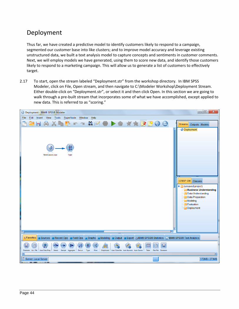
Deployment Thus far, we have created a predictive model to identify customers likely to respond to a campaign, segmented our customer base into like clusters; and to improve model accuracy and leverage existing unstructured data, we built a text analysis model to capture concepts and sentiments in customer comments. Next, we will employ models we have generated, using them to score new data, and identify those customers likely to respond to a marketing campaign. This will allow us to generate a list of customers to effectively target.

2.17 To start, open the stream labeled “Deployment.str” from the workshop directory. In IBM SPSS Modeler, click on File, Open stream, and then navigate to C:\Modeler Workshop\Deployment Stream. Either double-click on “Deployment.str”, or select it and then click Open. In this section we are going to walk through a pre-built stream that incorporates some of what we have accomplished, except applied to new data. This is referred to as “scoring.”

2.18 Double-click on the Type node. Note that, because this is current customer data, none of the fields have

their role set to Target.

2.19 From the Models palette, drag the Comments and Response with TEXT model nodes onto the canvas and

connect them to the Type node. Alternatively, copy and paste them from the Predictive Marketing Response SOLUTION stream.

2.20 From the Output palette, add a Table node to the canvas, connect it to the Response with TEXT model node, and select Run.

2.21 The new cases have been passed through the comments model to extract concepts, which were used as

inputs in the CHAID model to predict Response. The last two columns show the predicted outcome and the calculated confidence. For example, the first record in the table shown below is predicted to respond with 99% confidence.

2.22 Highlight one of the cells with the value of Responded. From the drop-down menu, select Generate and then choose Select Node (“Or”). This will generate a Select node on canvas. Alternatively, you can add a Select node form the Record Ops palette, and connect it to the Response model node.

2.23 Join the Generated node to the Response with TEXT model node. Double-click on the node to review the settings, where only those records predicted with a Responded prediction are selected. Click OK.

2.24 From the Record Ops palette, select a Sort node, and connect it to the Generated node. Double-click to edit the settings, sorting the confidence score field, $RC-Response, in descending order. Here we are sorting our customers predicted to respond by confidence in that prediction, from highest confidence to lowest. Click OK.

2.25 Returning to the Record Ops palette, select a Sample node, and connect it to the Sort node. Double-click the Sample node to edit the settings, sampling the first 100 records. Click OK.

2.26 Of interest to us now is a list or roster of those customers predicted most likely to respond to a campaign. Having sorted and sampled our current customers, we can effectively create a list of the top 100 customers to target for a marketing campaign. From the Export palette, select an Excel export node, and connect to the Sample node. Double-click to edit the settings. Change the File name to “Target List” in your local directory, and select “Launch Excel” before clicking on Run.

2.27 The result is actionable intelligence. That is, a list of the top 100 customer likely to respond to a marketing campaign that can be deployed to a decision maker.

3. Optimize Decisions 3.1 Launch Firefox by clicking on the FireFox icon at the bottom left of your screen, next to the Start button.

3.2 Once FireFox is open, click on the pushbutton labeled “ADM Portal” in Bookmarks Toolbar at the top of the FireFox window.

3.3 Enter “Admin” for the Username and if necessary use the Hot-Key combination, “Ctrl+P” to paste the preset password.

3.4 Once the logon credentials have been entered, click on the Login pushbutton.

If necessary, use the HotKey “Ctrl+P” to automatically paste the preset password

3.5 Once the IBM SPSS ADM is launched, you will be greeted with the Applications Launch page. Scroll down until

you see the application labeled “Campaign Optimization”.

3.6 Using the drop-down menu (shown above), select “retail_campaign.str” and click “Go”. This will open the Campaign Optimization application Home Screen, wherein you will see the interactive Project Steps interface, representing different steps in the optimization process; from choosing data through defining, deploying, and reporting on the results.

3.7 Before identifying which optimization scenario to use, let’s view the current project parameters. Using the interactive Project Steps interface, click on the database icon (shown above). Once in the Data tab, you’ll notice that the loaded data includes variables related to customer demographic and purchasing behavior.

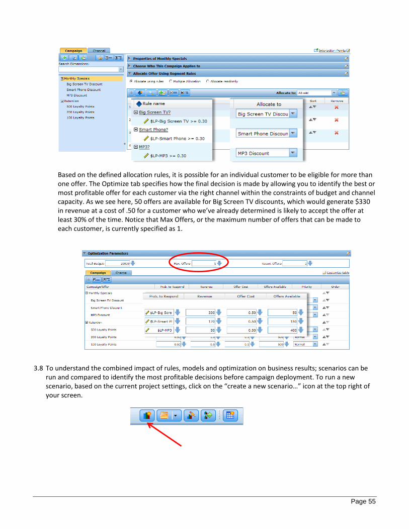
The Define tab specifies the rules and models that determine which customers are eligible for specific offers. For this project, there are two campaigns. Monthly Specials consist of discounts for various electronics. This is determined by a model that predicts acceptance of the offer with at least a 30% likelihood. The other campaign is Retention. This consists of loyalty points offered at incremental levels determined by the customer’s lifetime value. Allocation of each offer is determined by the defined Segment Rules.

Based on the defined allocation rules, it is possible for an individual customer to be eligible for more than one offer. The Optimize tab specifies how the final decision is made by allowing you to identify the best or most profitable offer for each customer via the right channel within the constraints of budget and channel capacity. As we see here, 50 offers are available for Big Screen TV discounts, which would generate $330 in revenue at a cost of .50 for a customer who we’ve already determined is likely to accept the offer at least 30% of the time. Notice that Max Offers, or the maximum number of offers that can be made to each customer, is currently specified as 1.

3.8 To understand the combined impact of rules, models and optimization on business results; scenarios can be run and compared to identify the most profitable decisions before campaign deployment. To run a new scenario, based on the current project settings, click on the “create a new scenario…” icon at the top right of your screen.

3.9 From within the New Scenario dialog, change the “Name” to Current Policy and select “Run”. This will run a Business Scenario Analysis on the project as it is currently defined.

3.10 The resulting output summarizes expected profit, budget, offers accepted, and other details. You’ll notice, for example, that for a budget of $248.44, the resulting profit from 685.72 accepted offers is projected to be $26,337.11.

3.11 Click on the Define step within the “Summary of Customer” to show results based on number of offers allocated. Viewed by Campaign, we see that 790 Monthly Specials and 2480 Retention offers were allocated.

3.12 To view allocations by offer, use the drop-down menu at the right to select “Offer” as Primary dimension and “Campaign” as Overlay dimension. The updated results indicate that, within the Retention campaign, the majority (1088) of allocated offers were for 100 Loyalty points. Within the Monthly Special campaign, the majority (378) of allocated offers were for MP3 discounts.

3.13 Click on the Optimize step within the “Summary of Customer” to show results based on offers that were actually made. That is, based on the current policy of allowing a maximum of 1 offer to be made to eligible customers, the actual offers made dropped considerably. Toggle the drop down menus to the right to reflect the same changes we made in the “Define” step

3.14 To assess the business impact of changing the current policy, exit the current scenario to return to the project workspace by clicking on the X at the upper right.

3.15 Return to the Optimize tab, change the max offers from 1 to 3. Eligible customers will now be made up to

3 offers.

3.16 Run a new scenario to see the business impact of this change on the results. Click on the “create a new scenario…” icon to open the New Scenario dialog box. Name this new scenario “3 Max Offers” and select “Run”.

3.17 The resulting output summarizes expected profit, budget, offers accepted, and other details.

3.18 To view both scenarios, run a side-by-side comparison. Click on the “compare up to…” icon at the top right.

3.19 Using the arrows at the center, drag both scenarios from the left box to the right and select “Compare”.

3.20 The side-by-side comparison shows the immediate impact of the policy change. Total Profit (Projected) between the first scenario in which each customer is made 1 offer and the second scenario in which each customer is made up to 3 offers resulted in a substantial increase.

3.21 Updating the chart metric to show Budget Spent reveals that the Total Profit (Projected) requires a minimal additional cost resulting in a significant return on investment.

3.22 Switching from graphical to tabular format provides a breakdown of the metrics between scenarios.

3.23 Click on the Optimize step within the “Summary of Customer.” This allows us to compare the optimization inputs (as specified in our project workspace) and the optimization outputs. Click on the “Optimization Outputs” tab. Here we see the metrics broken down by dimension.

3.24 Having run and compared scenarios, a decision regarding which campaign settings to move forward with can be made. Choosing to deploy the project with the highest projected profit, click on the “open an existing scenario” icon at the top right to return to the scenario “3 Max Offers”, which has automatically been saved.

3.25 Click on the following icon next to “3 Max Offers” at the top right, and choose “Continue” in the resulting dialog box. This will allow you to update the project workspace to reflect those of the currently selected scenario.

Your campaign is now ready to be put into production! We have just seen how leveraging business rules, predictive analytics and optimization within IBM SPSS Modeler Gold will result in optimized business decisions. With Business Scenario Analysis, we can immediately understand the business impact of changes by creating and comparing business scenarios.

Notices

This information was developed for products and services offered in the U.S.A. IBM may not offer the products, services, or features discussed in this document in other countries. Consult your local IBM representative for information on the products and services currently available in your area. Any reference to an IBM product, program, or service is not intended to state or imply that only that IBM product, program, or service may be used. Any functionally equivalent product, program, or service that does not infringe any IBM intellectual property right may be used instead. However, it is the user's responsibility to evaluate and verify the operation of any non-IBM product, program, or service. IBM may have patents or pending patent applications covering subject matter described in this document. The furnishing of this document does not grant you any license to these patents. You can send license inquiries, in writing, to: IBM Director of Licensing IBM Corporation North Castle Drive Armonk, NY 10504-1785 U.S.A. For license inquiries regarding double-byte (DBCS) information, contact the IBM Intellectual Property Department in your country or send inquiries, in writing, to: IBM World Trade Asia Corporation Licensing 2-31 Roppongi 3-chome, Minato-ku Tokyo 106-0032, Japan The following paragraph does not apply to the United Kingdom or any other country where such provisions are inconsistent with local law: INTERNATIONAL BUSINESS MACHINES CORPORATION PROVIDES THIS PUBLICATION "AS IS" WITHOUT WARRANTY OF ANY KIND, EITHER EXPRESS OR IMPLIED, INCLUDING, BUT NOT LIMITED TO, THE IMPLIED WARRANTIES OF NON-INFRINGEMENT, MERCHANTABILITY OR FITNESS FOR A PARTICULAR PURPOSE. Some states do not allow disclaimer of express or implied warranties in certain transactions, therefore, this statement may not apply to you. This information could include technical inaccuracies or typographical errors. Changes are periodically made to the information herein; these changes will be incorporated in new editions of the publication. IBM may make improvements and/or changes in the product(s) and/or the program(s) described in this publication at any time without notice. Any references in this information to non-IBM Web sites are provided for convenience only and do not in any manner serve as an endorsement of those Web sites. The materials at those Web sites are not part of the materials for this IBM product and use of those Web sites is at your own risk. IBM may use or distribute any of the information you supply in any way it believes appropriate without incurring any obligation to you. Any performance data contained herein was determined in a controlled environment. Therefore, the results obtained in other operating environments may vary significantly. Some measurements may have been made on development-level systems and there is no guarantee that these measurements will be the same on generally available systems. Furthermore, some measurements may have been estimated through extrapolation. Actual results may vary. Users of this document should verify the applicable data for their specific environment. Information concerning non-IBM products was obtained from the suppliers of those products, their published announcements or other publicly available sources. IBM has not tested those products and cannot confirm the

accuracy of performance, compatibility or any other claims related to non-IBM products. Questions on the capabilities of non-IBM products should be addressed to the suppliers of those products. All statements regarding IBM's future direction and intent are subject to change or withdrawal without notice, and represent goals and objectives only. This information contains examples of data and reports used in daily business operations. To illustrate them as completely as possible, the examples include the names of individuals, companies, brands, and products. All of these names are fictitious and any similarity to the names and addresses used by an actual business enterprise is entirely coincidental. All references to fictitious companies or individuals are used for illustration purposes only. COPYRIGHT LICENSE: This information contains sample application programs in source language, which illustrate programming techniques on various operating platforms. You may copy, modify, and distribute these sample programs in any form without payment to IBM, for the purposes of developing, using, marketing or distributing application programs conforming to the application programming interface for the operating platform for which the sample programs are written. These examples have not been thoroughly tested under all conditions. IBM, therefore, cannot guarantee or imply reliability, serviceability, or function of these programs.

Appendix A. Trademarks and copyrights

The following terms are trademarks of International Business Machines Corporation in the United States, other countries, or both:

IBM AIX CICS ClearCase ClearQuest Cloudscape

Cube Views DB2 developerWorks DRDA IMS IMS/ESA

Informix Lotus Lotus Workflow MQSeries OmniFind

Rational Redbooks Red Brick RequisitePro System i

System z Tivoli WebSphere Workplace System p

Adobe, Acrobat, Portable Document Format (PDF), and PostScript are either registered trademarks or trademarks of Adobe Systems Incorporated in the United States, other countries, or both. Cell Broadband Engine is a trademark of Sony Computer Entertainment, Inc. in the United States, other countries, or both and is used under license therefrom. Java and all Java-based trademarks and logos are trademarks of Sun Microsystems, Inc. in the United States, other countries, or both. See Java Guidelines Microsoft, Windows, Windows NT, and the Windows logo are registered trademarks of Microsoft Corporation in the United States, other countries, or both. Intel, Intel logo, Intel Inside, Intel Inside logo, Intel Centrino, Intel Centrino logo, Celeron, Intel Xeon, Intel SpeedStep, Itanium, and Pentium are trademarks or registered trademarks of Intel Corporation or its subsidiaries in the United States and other countries. UNIX is a registered trademark of The Open Group in the United States and other countries. Linux is a registered trademark of Linus Torvalds in the United States, other countries, or both. ITIL is a registered trademark and a registered community trademark of the Office of Government Commerce, and is registered in the U.S. Patent and Trademark Office. IT Infrastructure Library is a registered trademark of the Central Computer and Telecommunications Agency which is now part of the Office of Government Commerce. Other company, product and service names may be trademarks or service marks of others.

© Copyright IBM Corporation 2014. The information contained in these materials is provided for informational purposes only, and is provided AS IS without warranty of any kind, express or implied. IBM shall not be responsible for any damages arising out of the use of, or otherwise related to, these materials. Nothing contained in these materials is intended to, nor shall have the effect of, creating any warranties or representations from IBM or its suppliers or licensors, or altering the terms and conditions of the applicable license agreement governing the use of IBM software. References in these materials to IBM products, programs, or services do not imply that they will be available in all countries in which IBM operates. This information is based on current IBM product plans and strategy, which are subject to change by IBM without notice. Product release dates and/or capabilities referenced in these materials may change at any time at IBM’s sole discretion based on market opportunities or other factors, and are not intended to be a commitment to future product or feature availability in any way. IBM, the IBM logo and ibm.com are trademarks or registered trademarks of International Business Machines Corporation in the United States, other countries, or both. If these and other IBM trademarked terms are marked on their first occurrence in this information with a trademark symbol (® or ™), these symbols indicate U.S. registered or common law trademarks owned by IBM at the time this information was published. Such trademarks may also be registered or common law trademarks in other countries. A current list of IBM trademarks is available on the Web at “Copyright and trademark information” at ibm.com/legal/copytrade.shtml Other company, product and service names may be trademarks or service marks of others.

ibm spss predictive analytics workshop spss predictive analytics workshop ... 1.8 from the drop-down...

Documents